The CLAS12 Superconducting Magnets
58
> NIM-A Format version (2019) magnets_RF34j 1 1 The CLAS12 Superconducting Magnets R. Fair a,1 , N. Baltzell a , R. Banchimanchi a , G. Biallas b , V.D. Burkert a , P. Campero-Rojas a , L. Elementi c , L. Elouadrhiri a , B. Eng a , P. K. Ghoshal a , J. Hogan a , D. Insley a , V. Kashikhin c , D. Kashy a , S. Krave c , O. Kumar a , M. Laney a , R. Legg b , M. Lester a , T. Lemon a , A. Lung a , C. Luongo e , J. Matalevich a , M.D. Mestayer a , R. Miller a , W. Moore a , J. Newton a , F. Nobrega c , O. Pastor e , S. Philip a , R. Rajput-Ghoshal a , V. Rao Ganni g , C. Rode b , N. Sandoval a , S. Spiegel a , D. Tilles b , K. Tremblay a , G. Velev c , C. Wilson a , M. Wiseman a , G.R. Young b a Thomas Jefferson National Accelerator Facility (TJNAF), Newport News, VA, 23606, USA b Thomas Jefferson National Accelerator Facility, Newport News, VA, 23606, USA (Retired) c Fermi National Accelerator Laboratory (FNAL), Batavia, IL,60510 USA d SLAC National Accelerator Laboratory, Stanford, CA, 94025 USA (Previously with TJNAF) e International Thermonuclear Experimental Reactor Organization (ITER), St. Paul-lez-Durance 13067, France (Previously with TJNAF) f CEA Saclay, F91191 Gif-sur-Yvette, France g Michigan State University, East Lansing, MI, 48824 USA (Previously with TJNAF) h Old Dominion University, Norfolk, VA, 23529, USA ARTICLE INFO ABSTRACT Keywords: Superconducting, magnets, torus, solenoid, quench, mapping , toroid As part of the Jefferson Lab 12 GeV upgrade, the Hall B CLAS12 system requires two superconducting iron-free magnets – a torus and a solenoid. The physics requirements to maximize space for the detectors guided engineers toward particular coil designs for each of the magnets which, in turn, led to the choice of using conduction cooling. The torus consists of 6 trapezoidal NbTi coils connected in series with an operating current of 3770 A. The solenoid is an actively shielded 5 T magnet consisting of 5 NbTi coils connected in series operating at 2416 A. Within the hall, the two magnets are located in close proximity to each other and are completely covered both inside and outside by particle detectors. Stringent size limitations were imposed for both magnets and introduced particular design and fabrication challenges. This paper describes the design, construction, installation, commissioning, and operation of the two magnets. 1 The Manuscript received XXXXXX. This work was supported by Jefferson Science Associates, LLC, under U.S. DOE Contract DE-AC05-06OR23177. The U.S. Government retains a non- exclusive, paid-up, irrevocable, world-wide license to publish or reproduce this manuscript for U.S. Government purposes. Corresponding author: R Fair (e-mail: [email protected]) Color versions of one or more of the figures in this paper are available online at XXXXXXXX Digital Object Identifier (inserted by Publisher)
Transcript of The CLAS12 Superconducting Magnets

> NIM-A Format version (2019) magnets_RF34j
1
1
The CLAS12 Superconducting Magnets
R. Faira,1, N. Baltzella, R. Banchimanchia , G. Biallasb, V.D. Burkert a, P. Campero-Rojasa, L. Elementic, L. Elouadrhiria, B.
Enga, P. K. Ghoshala, J. Hogana, D. Insleya, V. Kashikhinc, D. Kashya, S. Kravec, O. Kumara, M. Laneya, R. Leggb, M. Lestera, T.
Lemona, A. Lunga, C. Luongoe, J. Matalevicha, M.D. Mestayera, R. Millera, W. Moorea, J. Newtona, F. Nobregac, O. Pastore,
S. Philipa, R. Rajput-Ghoshala, V. Rao Gannig, C. Rodeb, N. Sandovala, S. Spiegela, D. Tillesb, K. Tremblaya, G. Velevc, C.
Wilsona, M. Wisemana, G.R. Youngb
a Thomas Jefferson National Accelerator Facility (TJNAF), Newport News, VA, 23606, USA b Thomas Jefferson National Accelerator Facility, Newport News, VA, 23606, USA (Retired) c Fermi National Accelerator Laboratory (FNAL), Batavia, IL,60510 USA d SLAC National Accelerator Laboratory, Stanford, CA, 94025 USA (Previously with TJNAF) e International Thermonuclear Experimental Reactor Organization (ITER), St. Paul-lez-Durance 13067, France (Previously with TJNAF) f CEA Saclay, F91191 Gif-sur-Yvette, France g Michigan State University, East Lansing, MI, 48824 USA (Previously with TJNAF) h Old Dominion University, Norfolk, VA, 23529, USA
ARTICLE INFO ABSTRACT
Keywords: Superconducting, magnets, torus, solenoid,
quench, mapping , toroid
As part of the Jefferson Lab 12 GeV upgrade, the Hall B CLAS12 system
requires two superconducting iron-free magnets – a torus and a solenoid. The
physics requirements to maximize space for the detectors guided engineers
toward particular coil designs for each of the magnets which, in turn, led to the
choice of using conduction cooling. The torus consists of 6 trapezoidal NbTi
coils connected in series with an operating current of 3770 A. The solenoid is
an actively shielded 5 T magnet consisting of 5 NbTi coils connected in series
operating at 2416 A. Within the hall, the two magnets are located in close
proximity to each other and are completely covered both inside and outside by
particle detectors. Stringent size limitations were imposed for both magnets
and introduced particular design and fabrication challenges. This paper
describes the design, construction, installation, commissioning, and operation
of the two magnets.
1 The Manuscript received XXXXXX.
This work was supported by Jefferson Science Associates, LLC, under U.S. DOE Contract DE-AC05-06OR23177. The U.S. Government retains a non-exclusive, paid-up, irrevocable, world-wide license to publish or reproduce this manuscript for U.S. Government purposes.
Corresponding author: R Fair (e-mail: [email protected]) Color versions of one or more of the figures in this paper are available online at XXXXXXXX
Digital Object Identifier (inserted by Publisher)

> NIM-A Format version (2019) magnets_RF34j
2
2
I. PHYSICS REQUIREMENTS AND TECHNICAL SPECIFICATIONS
The CEBAF Large Acceptance Spectrometer for 12 GeV
(CLAS12) is a new detector system within Hall B at Jefferson
Laboratory (JLab) designed to measure electron-induced
reactions over a broad kinematic phase space. It consists of two
large superconducting magnets, a 6-coil torus and a 5-coil
solenoid. The solenoid magnet is located upstream of the torus
magnet and provides a field to bend low-energy (300 MeV to 1.5
GeV) charged particles. The field also provides focusing and
shielding for Møller electrons, which allows the detector system
to run at high data rates. A homogeneous field at the magnet
center is needed for polarized targets. The torus provides a
bending field for high energy (0.5 GeV to 10 GeV) charged
particles and mechanical support for 3 regions of drift chambers.
A general overview of the physics requirements and experiment
design in provided in Ref. [1].
Tables I and II summarize the physics requirements for the torus
and solenoid superconducting magnets, respectively, while Table
III provides a summary of the key design parameters for the two
magnets. Figure 1 illustrates the locations of the two magnets
relative to each other while Fig. 2 shows photographs of the two
magnets.
Figure 1: Simplified model illustrating the locations of the solenoid and the
torus with respect to each other (no physics detectors are shown here).
TABLE I CLAS12 HALL B - TORUS PHYSICS REQUIREMENTS
Parameters Requirement
Angular coverage
(cone angle relative to the
forward direction)
= 50 - 400
ΔØ = 50-90% of 2π
∫B.dl @ nominal current 2.83 T.m @ = 50
0.6-1.0 T.m @ = 400
Access Open access to field volume on either side of
beamline
TABLE II
CLAS12 HALL B – SOLENOID PHYSICS REQUIREMENTS
Parameters Requirement
B0 5 T
L=1/B0∫Bdl L = 1 to 1.4 m
Field uniformity in target Area
ΔB/B0 < 10-4 in cylinder 0.04 m length x 0.025 m (100 ppm)
Field at HTCC PMTs B < 35 G (for the four HTCC PMT locations) [2]
Field at CTOF PMTs B < 1200 G (for the two CTOF PMT locations) [3]
HTCC – High Threshold Cherenkov Counter, CTOF – Central Time of Flight,
PMT – Photomultiplier Tubes
TABLE III
CLAS12 HALL B - SOLENOID AND TORUS MAGNET PARAMETERS
PARAMETER DESIGN VALUE
SOLENOID TORUS
Number of Coils
2 + 2 + 1 (2 inner + 2 intermediate +
1 outer shield)
6
Coil design Helically layer-wound
potted coils Double pancake potted in
aluminum case
Total number of turns 5096
2 x 840 + 2 x 10¹²+1392 1404 (117 x 2 x 6)
NbTi Rutherford cable SSC 36 strands SSC 36 strands
Nominal current (A) 2416 3770
Central field (T) 5 N/A
Conductor peak field (T) 6.56 3.6
Required field homogeneity
1 x 10⁻⁴
Over a ɸ25mm x L40 mm cylindrical volume at
magnetic center
N/A
Inductance (H) 5.89 2
Stored energy (MJ) 17 14
Warm bore (mm) 780 124
Outer diameter x length 2.16 m x1.8 m N/A
Inner bore length /opening
angle 0.897 m/410 N/A
Coil case thickness - Originally 100mm changed to
125mm
Total weight (kg) 18800 25500
Cooling mode Conduction cooled Conduction cooled
Supply temperature (K) 4.5 4.5
Temperature margin (K) 1.5 1.5
Stabilized conductor W17 mm x T2.5 mm
copper channel
W20 mm x T2.5 mm copper
channel
Turn-to-turn insulation 0.004” glass tape ½ Lap 0.003” glass tape ½ lap
Heat shield cooling Helium boil-off LN2 thermo-siphon
The torus magnet and the Torus Service Tower (TST) were
designed and built at JLab; the Cryogenic Distribution Box
(DBX), was designed at JLab and fabricated by Meyer Tool,
while the coils were fabricated at the Fermi National Accelerator
Laboratory (FNAL), USA [4, 5]. The solenoid magnet was
designed and fabricated by Everson Tesla Inc., USA (ETI), while
the Solenoid Service Tower (SST) and cryogenics were designed
and fabricated by JLab. The magnets differ in their cooling
schemes from that of more conventional bath-cooled
superconducting magnets by using conduction-cooling
methodology in order to comply with tight physical space

> NIM-A Format version (2019) magnets_RF34j
3
3
requirements. These requirements imposed certain size
limitations on the design of the torus and solenoid magnet coils,
which led to each magnet having their own unique issues for
design, fabrication, installation, and control [6]. Leftover NbTi
Rutherford superconductor cable from the Superconducting
Super Collider (SSC) project (which was terminated in 1993) was
modified by soldering the cable into a C-shaped copper channel
and then used to wind the coils for both the torus and solenoid.
Figure 2: Magnets installed in Hall B – (a) Solenoid (with some detectors installed), (b) Torus (before drift chambers were installed between the coils).
II. PROJECT MANAGEMENT AND RISK MITIGATION APPROACH
The Hall B torus and solenoid magnets were part of the JLab 12
GeV Upgrade project, which included an upgrade to the
accelerator and three of the four experimental Halls B, C, and D.
The project involved the fabrication, installation, and
commissioning of a total of 8 superconducting magnet systems
[7]. Once the majority of the design work had been completed, a
Magnet Task Force was set up at JLab in order to provide
consistency in the management of the various activities, to
promote the sharing of lessons learned between the different
magnet systems and halls, and to provide a more focused effort.
The task force leader had overall technical responsibility for all
the magnets, including the Hall B torus and solenoid magnets, and
oversaw the timely completion of all tasks. Key procurements (for
example individual magnets and magnet power supplies) were
overseen by the respective Subcontracting Officers (SOs) from
the JLab Procurement Department with technical assistance being
provided by Subcontracting Officer Technical Representatives
(SOTRs). Multiple design and manufacturing reviews were held
for each magnet and other key components, most of which were
face to face. Progress tracking, problem-solving meetings, and
teleconference calls were held with the various vendors on either
a regular schedule or on an as-needed basis. JLab staff also
provided oversight at the vendors’ premises, especially during
key manufacturing stages.
All critical tasks and systems of the magnets of the CLAS12
system, both torus and solenoid, were subjected to a detailed Risk
Assessment and Mitigation (RAM) process. The process was used
to evaluate the overall magnet design and the robustness of its
protection system and commissioning process. The magnet risk
assessments were developed via a series of electromagnetic and
electromechanical analyses, which included induced eddy
currents, Lorentz forces, thermal loading, magnet-to-magnet
interactions, and an assessment of magnet performance while in
proximity to ferromagnetic structures. The assessments also
included things like loss of control power, loss of main power,
loss of cryogenic supply, and loss of vacuum. The risk mitigation
approach was based on a Failure Modes and Effects Analysis (FMEA) carried out for each phase of the project: design,
fabrication, installation, and commissioning [8]. FMEA is a tool
used to eliminate or mitigate known potential failures, problems,
and errors within systems. A failure mode is defined as the way a
component could fail to meet its performance requirements or to
function. More than 400 risk items were identified, categorized,
and ranked; mitigation avenues were investigated for all risks, and implemented when warranted, either because the risk was
deemed to be high, or implementation was easily achieved.
The potential failure modes were evaluated based on a Risk
Priority Number (RPN), which is the product of three factors: the
Severity ranking (S), the probability of Occurrence (O), and the
probability of Detection (D). The RPN was used as a measure of
overall risk and helped to identify and rank the risks of the
potential failure modes. The end results of failures that lead to
unsafe conditions or significant losses in functionality were rated
high in severity. Larger RPNs indicated the need for corrective
action or failure resolution. The FMEA process was used to assist
in identifying potential failure modes early in the design phase.

> NIM-A Format version (2019) magnets_RF34j
4
4
Several of the key risks for the torus and solenoid (indicated by
larger RPNs) are listed below and were addressed during the
project:
The system does not satisfy the physics requirements;
Late delivery of key components and subsystems from
vendors;
Defects in the build and manufacture of thermal insulation
(e.g. standoffs, multi-layer insulation);
Insufficient helium mass flow in the cooling channel;
Vacuum vessel cannot maintain required vacuum;
Breakdown of the electrical insulation of the magnet system;
Loss of control of the magnet power supply system;
Loss of magnet protection due to a fault in the quench
detection and protection system.
Some of the mitigation actions stemming from the FMEA included:
Extensive use of mock-ups and practice builds for all quality-
critical activities (e.g. conductor soldering into channel,
conductor splices, distortion of vacuum jackets during
welding, connection of hex beams to coils, mounting of
instrumentation);
Development of written procedures, before and in
conjunction with the practice builds;
Safety and risk-awareness meetings prior to each critical
operation;
Extensive use of in-process quality assurance (QA) checks;
Detailed weekly and daily planning of installation activities
in the hall;
Vendor oversight by JLab staff.
Safety reviews, as well as Director’s Reviews, Magnet Advisory
Group Meetings, and U.S. Department of Energy Reviews, played
a crucial role in developing the RAM process at JLab, as well as
to guide the technical path, verify resources, and check project
progress. Safety reviews in particular comprised two key sub-
reviews - Pressure System Reviews (which checked against
relevant design codes like ASME and also ensured all relevant
documentation was in place), and Experimental Readiness
Reviews (Cool down and Power-up reviews) before the magnet
systems were signed over to the JLab Physics Division for
operation.
III. DESIGN AND ANALYSIS
The coils for the two magnets utilized surplus Superconducting
Super Collider (SSC) outer dipole conductor that consisted of 36
strands of 0.65-mm diameter multi-filament NbTi superconductor
with a Cu:Sc ratio of 1.8:1, manufactured as a key-stoned
Rutherford cable and soldered into a rectangular nominally
dimensioned 2.5 mm × 20 mm OFHC copper channel for the torus
and a 2.5mm x 17 mm channel for the solenoid (see Fig. 3 and
Table IV for details). This Rutherford conductor had been in
storage for many years, so sample lengths of conductor from each
spool were tested to check for any degradation in performance.
The superconductor for the magnets has a tested short sample
performance of better than 11000 A at 4.2 K at 5 T and showed
no discernable degradation when compared to its original
specifications. The cable and copper channel underwent rigorous
inspection and cleaning processes prior to being soldered
together. These were time-consuming and laborious processes.
Figure 3: SSC Outer Dipole NbTi Rutherford Cable and cross-sectional view of the conductor with critical dimensions shown for the torus conductor.
TABLE IV
TORUS CONDUCTOR SPECIFICATION
TORUS
Torus Magnet Design
The torus magnet has 6 double-pancake, trapezoidal-shaped coils
wound with copper-stabilized NbTi Rutherford cable, which were
vacuum impregnated with epoxy, wrapped with copper cooling
sheets, assembled in aluminum cases, and then epoxy-
impregnated a second time, to produce a coil cold mass (CCM)
that operates at 4.5 K. Pre-formed multi-layer insulation (MLI)
blankets were fitted to each CCM (see Fig. 4).
Parameter Details
Rutherford type of cable (Superconductor) NbTi
Conductor material (NbTi + Cu) Cu-(NbTi) in rectangular
Cu channel
Number of strands in the cable 36
Number of NbTi filaments in each strand 4600
Strand bare diameter (mm) 0.648
Copper to non-copper ratio 1.8
Twist pitch (mm) 15
Conductor size (bare) (mm x mm) 20 x 2.5
Conductor size (insulated) (mm x mm) 20.2 x 2.7
Minimum Short sample current at 4.22 K, 5 T (A) >11000
RRR Cu (Cu-NbTi) – Strand 100
Minimum RRR Cu channel (design) 70

> NIM-A Format version (2019) magnets_RF34j
5
5
Figure 4: A torus magnet coil in its vacuum jacket.
Aluminum thermal shields, (cooled to 80 K by a liquid-nitrogen
thermo-siphon), surround each CCM and themselves were
covered with additional MLI blankets. The whole assembly is
enclosed within a welded stainless-steel vacuum jacket. The 6
independent CCMs are mechanically held together at a cold hub
positioned along the axis of the torus. The CCMs are connected
to each other on their outer extremities via 12 hex beams, which
are conduction cooled to 4.5 K. There are two hex beams per
sector, upstream and downstream (see Fig. 5).
Figure 5: The torus magnet - key features, dimensions, and heat loads.
The six coils are electrically connected in series using soldered
joints (splices). The system has three hydraulic circuits all
supplied by the Torus Service Tower (TST) – supercritical helium
to indirectly cool the coils, atmospheric helium running through
the re-coolers and a liquid-nitrogen circuit for the thermal shields.
A liquid-filled (4.5 K, 1.4 atm) helium re-cooler (tube-in-shell
heat exchanger) is mounted to each upstream hex beam. The coil-
to-coil splices are mounted to and cooled by these re-coolers. The
re-coolers remove heat input at each coil before entering the next
coil and thus maintain equal helium inlet temperatures to each
coil. A small fraction of the boil-off from the re-coolers is used to
cool the magnet’s vapor-cooled current leads, the rest is sent back
to the refrigerator. All six coils share a common vacuum space
with two vacuum pumping systems being operated continuously
- at the top and bottom of the torus magnet. A single distribution
box (DBX) supplies both the torus and the solenoid magnets.
Torus Superconducting Coil Design
The torus magnet coils generate a toroidal magnetic field. The
∫B.dl requirements outlined in Table I require a trapezoidal coil
shape to be used. Figure 6a illustrates the magnetic field
distribution on the coil surface. The peak field of 3.6 T is located
at the coil inner bore surface and is almost half this value at the
coil’s outer radius. Figure 6b indicates the temperature
distribution across the coil, with the “warmest” part of coil having
the highest thermal radiation heat load near the lead exit due to
the extended surface of the coil case at the hex rings.

> NIM-A Format version (2019) magnets_RF34j
6
6
Figure 6: (a) Magnetic field distribution on the torus coil surface with the magnet at 3770 A. (b) Steady state temperature distribution on the torus coil surface (assuming 3x design heat load).
Figure 7 summarizes the performance of the superconducting
Rutherford cable used for both the torus and solenoid magnets in
the form of a set of critical current curves at varying operating
temperatures. The load lines for the torus and solenoid magnets
are displayed as straight lines labeled Icoil.
1
Figure 7: Superconducting Rutherford cable critical current vs. magnetic flux density– solenoid and torus magnet load lines (Icoil).
(Note: the peak field calculation includes the detailed cable and strand geometry)
An assessment of the conductor stability for the torus is summarized in Table V.
TABLE V
SUMMARY OF TORUS CONDUCTOR STABILITY ASSESSMENT
Several scenarios were evaluated during the design phase for
different coil operating temperatures, different local magnetic field magnitudes, and also an examination of the effect of losing 2 out of the 36 strands from the conductor. As can be seen from
Fig. 6 and Table VI, the torus coil design has a more than
adequate temperature margin ∆T, which in all cases exceeds the
usual design guidance of 1.5 K, suggesting that the magnet coils
are somewhat tolerant, in particular, to temperature variations [9].
Case #1: Operating temperature (Top) 4.7 K (1st
pancake), Bmax
Case #2: Top=4.9 K (2nd pancake), Bmax
Case #3: Top =5.3 K (2nd pancake), Bmax
Case #4: Top =5.3 K (2nd pancake), Bmax (assuming 2
lost strands)
Operating Scenario (Hall B Torus)
Conductor temperature Top (K) 5.3 K Maximum field in the coil Bmax (T) 3.58 T
Operating current Iop (A) 3770 A
Ic (at Bmax) (A) at Top 9836
Summary
Short sample performance (SSP) < 40% 38.33%
Stable for Tcs value (Margin) Yes >1.5 K
Stable for Beta (Adiabatic stability) Yes
Adiabatic flux jump stability Yes
Dynamic stability Yes
Adiabatic self-field stability Yes
Stable in term of twist pitch Yes
Stable for finite element size Yes

> NIM-A Format version (2019) magnets_RF34j
7
7
Case #5: Top =5.9 K (2nd pancake), B = 1.5 T (lead exit)
TABLE VI
TORUS MAGNET MARGIN AND SSP
Case Bmax
(T)
Ic (at Bmax)
(A) at Top Iop (A)
%
SSP
Top
(K)
Tc
(K)
Tg
(K)
∆T (K) = Tg(K) –
Top(K)
1 3.58 12076 3770 31.22 4.7 7.86 6.87 2.17
2 3.58 11332 3770 33.27 4.9 7.86 6.88 1.98
3 3.58 9836 3770 38.33 5.3 7.86 6.88 1.58
4 3.58 9285 3770 40.60 5.3 7.86 6.82 1.52
5 1.5 11467 3770 32.88 5.9 8.75 7.81 1.91
The coil turn insulation, pancake-to-pancake insulation, and the Turn-to-Ground insulation was designed as shown in Fig. 6 to meet the requirements in Table VII. A similar approach was used
to define the solenoid coil insulation. The magnet coils are
protected via an externally located dump resistor that is
permanently connected across the magnet terminals. This resistor has a center tap that then feeds a ground-fault indicator. The
presence of this center tap produces an expected maximum voltage across the magnet during a typical quench scenario of
250 V. However, in the extremely unlikely event that the center tap is lost, the voltage across the magnet terminals could increase
to a peak of approximately 500 V. This hardware-related fault voltage, together with a safety factor, as well as a full protection analysis to calculate coil peak temperatures and voltages, was
used to determine the overall design for the coil turn insulation, pancake-to-pancake insulation, and the Turn-to-Ground
insulation (see Fig. 8 and Table VII) [9].
Figure 8: Partial construction detail for the torus coils, showing the conduction cooling mechanism and coil winding details. The coil cross section inside of the
aluminum case is 353 x 45 mm.
TABLE VII TORUS COIL ELECTRICAL INSULATION BREAKDOWN VOLTAGE
Material E-Glass
with Epoxy G10 Kapton
Insulation Region Thickness
(mm)
Thickness
(mm)
Thickness
(mm)
Turn-to-Turn Insulation (T-T) 0.3048 0 0
Turn-to-Turn Insulation (between pancakes)
0.3048 0.38 0
Turn-to-Ground (GND) 0.508 0 0.1524
Location Turn-to-
Turn
Pancake-
Pancake Turn-to-GND
Breakdown Voltage (kV) -calculated
7.01 15.75 kV 21.74 kV
Factor of safety 101 101 51
Breakdown voltage (kV) with
safety factor used for design 0.7 1.58 4.35
Torus magnet 12 GeV
(V)_expected < 10 < 120 < 250*
1 Use safety factor of 5 where Kapton is used and 10 if no Kapton is used. [9]
* Rare hardware fault case resulting in approximately 500 V across the dump
resistor
Electromagnetic and structural analyses of the coil pack and coil case assembly were carried out. The analyses focused on the cool down process, normal operation at full operating current (which
also included gravity loads), as well as on conditions arising from coil misalignment, current imbalances, and quench events, to
ensure that the aforementioned components were all within acceptable stress limits (see Table VIII) [8, 9-14].
TABLE VIII
TORUS STRESS SUMMARY
Component
Primary
Limit
(MPa)
Primary +
Secondary
Limit(MPa)
EM + Gravity [Primary]
(MPa)
Cool down + EM
[Primary + Secondary] (MPa)
Peak General Peak General
Case 184 552 350 70 380 300 Cover 184 552 130 45 430 350
Conductor 94 282 - 68 - -181
Coil Pack Shear
15 45 5 13 40 20
Coil Pack
Radial 94 282 - -30 - -120
Primary stresses were limited to the lesser of 2/3 times the yield strength or 1/3 times the ultimate tensile strength. Primary plus secondary stresses were limited
to 3 times the primary stress allowable.
Torus Splice Design
The key drivers for the splice design were minimization of overall
splice resistance, (which necessarily included contact resistance),
and adequate quench protection. All conductors that are not
within the main coil winding, (splices between the individual
superconducting magnet coils, conductors between coils and
current leads, and long runs of superconducting bus bar), have
additional copper stabilizer to manage temperature rises during a
quench event. The conductors that enter and exit the coil case also
have stabilizer that runs to the outermost turn of each pancake. To
design a “quench-tolerant” splice, the amount of copper has to be
large enough to minimize peak temperatures during a quench
event but also small enough to allow the development of a
resistive voltage that can be detected and used to trip the fast
dump interlocks to prevent the superconductor from burning out
[15]. This “balancing act” is a critical part of the design of the
quench protection system of any superconducting magnet. The
Oxygen Free High Conductivity (OFHC) copper stabilizer bars
extend over the entire splice length and are soldered to the
assembly in the same operation that solders the splice.
To allow for a suitable design margin, the operating temperature
of the splice has been assumed to be 5 K instead of 4.5 K. Using
guidance from CERN, a joule heating limit (per splice) of 100
mW was selected, resulting in a maximum resistance of 7×10⁻⁹ Ω
per splice [15]. This resistance corresponds to an operating
current of 3770 A at 4.6 K with a background magnetic field in
the region of 0.3 T, allowing for the magnetoresistance in copper.

> NIM-A Format version (2019) magnets_RF34j
8
8
Splices are cooled via copper braids soldered to the helium re-
cooler units located inside the upstream cold hex beams and they
utilize a similar electrical insulation recipe to that used for the
coils. Space on the re-cooler units is limited and this constrained
the allowable size of the splice design.
The key risk to the joint is the lack of even solder distribution and
the inadvertent creation of voids within the solder and between
the cables being joined. The cables are placed with the SSC cables
facing each other and the keystone edges of the mating conductors
lying on opposite sides of the joint to ensure a minimum gap
between the cables. Several splice mock-ups were made and
destructively tested to qualify the soldering fixture and fabrication
procedure. A portion of the lip of the copper channel along the
mating surfaces of the two conductors was removed to reduce the
likelihood of void formation since the groove in the channel is
deeper than the thickness of the Rutherford cable (see Fig. 9).
Figure 9: (a) Torus conductor - SSC outer cable soldered into a copper channel
(dimensions in mm), (b) Typical layout of the test splice for joint resistance
evaluation (without additional copper stabilizer).
Sn60Pb40 solder, having a liquidus of 188 oC to 190 oC, (and a
melting point above 200 oC), was used to bond the Rutherford
cable into the copper channel. Soft solder paste Sn63Pb37 (with a
eutectic melting point of 183 oC) was used for the splice.
Delamination of the Rutherford cable from the copper channel
was avoided by careful control of the temperature during the
soldering process using thermocouples for monitoring. The
design of the soldering rig shown in Fig. 10 included open zones
for direct viewing of the conductors during soldering, which
allowed visual inspection of solder flow during the splicing
operation.
Figure 10: (a) Temperature-controlled aluminum block splicing rig. Cut-outs in the side of the rig allowed for visual inspection of solder flow, (b) Splice mock-
up end-on view of the sectioned splice cut lengthwise showing void-free
construction. NbTi strands and solder can be seen in the copper matrix. The outer-wrap is polyimide film and epoxy.
The splice insulation system is designed to accommodate a 2.5 kV
standoff to ground (when cold) and incorporates polyimide film
and a minimum tracking length of 1/2 inch. To improve thermal
performance, physical gaps in the assembly were filled with two-
part blue Stycast 2850 FT epoxy. The assembly was hi-pot tested
(conductor-to-ground) only to 1 kV in air at atmospheric pressure
to validate electrical isolation and integrity, as the full 2.5 kV
standoff was designed to allow for any variation in the application
of the insulation during the build of the magnet in the somewhat
cramped conditions in the hall. This allows for a more than
adequate safety margin.
Test splices with 360-mm-long soldered joints were prepared at
JLab and critical current (IC), n-value, and V-I data measurements
were carried out at the University of Durham, UK up to 2000 A
in one of two 15 T magnet systems (see Table IX). Due to a
limitation of the measurement set up that could not accommodate
the full length of the splice in the magnet, the resistance across the
splice was also measured at a lower current and in an elevated
magnetic field at LHe temperature. This additional measurement
was carried out to allow characterization of similar splices for the
Hall B solenoid magnet, that were likely to be located in higher
fields of up to 4 T. Typical resistances measured for sample
DR4686 are given in Table X.
TABLE IX CRITICAL CURRENT AND N-VALUE DATA FOR JLAB SPLICE SAMPLE# DR4562
Critical Current data
E field criteria 10.5 T 10.0 T 9.5 T
100 µV/m 254 A 851 A 1708 A
10 µV/m 165 A 656 A 1415 A
n-Value
10-100 µV/m 5 9 12
TABLE X
RESISTANCE MEASURED FOR DR4686 AT VARYING MAGNETIC FIELD AT 4.2 K
Joint Length
(mm)
Field at Field
Centre (T)
Field at the top of
the Joint (T)
Joint Resistance
(×10-9Ω)
260 0 0 ≤ 0.1
0.5 0.13 0.70 1 0.25 0.66
2 0.50 0.68
3 0.75 0.68 4 1 0.7
The resistance of the splices measured at elevated magnetic fields
was less than 1 nΩ in LHe (4.2 K), the maximum allowed design
value was 7.0 nΩ. This splice design and associated insulation
system, proven for the torus magnet, was shared with the vendor
for the solenoid magnet who implemented a very similar system.
Torus Quench Protection Design
The torus magnet is protected via an externally located dump resistor that is permanently connected across the magnet
terminals. This resistor has a center tap that then feeds a ground-fault indicator (see Fig. 12). Quench detection is via voltage taps located on either side of the splices between coils, thus allowing

> NIM-A Format version (2019) magnets_RF34j
9
9
voltage detection across individual coils, splices, and long runs of bus bar.
At the operating current of 3770 A and with a total inductance of
about 2 H, the torus magnet has a stored energy of 14.2 MJ. With
the 0.124 Ω dump resistor in circuit, any current decay under non-
quench conditions will have a time constant of 16.7 s, with the
magnet therefore running down to almost zero amps in about 5
time constants or 83.5 s. It should be noted that even during a
“normal” fast discharge of current into the dump resistor (for
example an interlock activating due a non-quench event)
sufficient eddy current heating can be produced, which in turn
would initiate a quench-back event that could then initiate a
quench in one or all of the coils. During the quench event
nonlinear superconductor normal zone growth and induced eddy
currents in the aluminum cases and shields will decrease the
effective discharge time due to the increase in effective resistance
in the overall magnet circuit.
Figure 12: Torus magnet protection circuit.
Reference should also be made to Table IV for the conductor
specification.
TABLE XI
BRIEF SUMMARY OF CALCULATED CRITICAL PARAMETERS
(TORUS)
Parameter (calculated) COIL
Operating temperature, Ɵ0 (K) 4.90
Current sharing temperature (K) 7.46
Temperature margin (K) 2.16
Short sample performance (%) at Ɵ0 27.1
MQE (mJ) 49
Conductor length used for quench calculation
(m)
2200 (per
coil) 1 Hot spot temp. (K) / Time to reach the
corresponding hot spot temperature (s) 52 K / 60.68 s
Max. voltage, Line-to-Ground (kV) > 2.5
Max. MIITs at 150 K (106.A2.s) 149.6
Dump resistor, RD (Ω) 0.124 2 Maximum voltage across the RD (V) 467
MIITs estimated with dump resistor (106.A2.s) 77.2
Normal magnet time constant (τ), s 16.1 1All energy dumped in one coil (adiabatic condition) 2 Maximum voltage across the RD for the worst case scenario =
approximately 500 V as designed (with center tap present, dump
resistor voltage = 250 V)
Design and Selection of a Dump Resistor (RD) for the Torus
An equivalent single-coil Wilson model [16] is used for quench
analysis. The stored energy of the torus magnet is ~14 MJ and is
to be extracted via an external dump resistor to limit the maximum
voltage to no higher than approximately 500 V in the event of a
fast discharge or a quench.
1. The maximum design voltage limit of approximately 500 V
was determined iteratively, via analysis of peak temperatures
and voltages, as well as by including consideration of the
hardware-related fault scenario with the center-tapped dump
resistor, and necessitated the use of a 124 mΩ external dump
resistor.
2. The magnet time constant was calculated to be: (LMagnet = 2.0
H), τ = LMagnet/RD = 2.0 H /0.124 Ω = 16.13s.
3. Table XI summarizes the critical parameters calculated for
the magnet coil with a maximum hot spot temperature limited
to no higher than 150 K. The adiabatic quench integral (also
referred to as MIITs)
a. Maximum MIITs calculated, MIITsmax = 149.6 MA2s
b. MIITs with RD, MIITsdump = 77.2 MA2s
c. MIITs without RD, MIITsno-dump = 236.8 MA2s
Note:
MIITs calculated with and without RD are based on the energy
extracted and on the time constant. The assumption and
calculations are:
a. The resistance of each coil (each CCM) above quench
temperature is assumed to be, rcoil = 10 mΩ;
b. To keep the peak temperature to below 150 K, the decay
time must be shorter than 10.53 s. The time constant with dump resistor during discharge, τ_RD =
LMagnet/(RD + rcoil*6) = 10.87 s
MIITs with RD, (1/2)*(IOP2/106)* [LMagnet/(RD + rcoil*6)] = 77.2
MA2s
The time constant without dump resistor during discharge,
τ_no_RD = LMagnet/rcoil*6 = 33.33 s
MIITs without RD, (1/2)*(IOP2/106)* (LMagnet/rcoil*6) = 236.8 MA2s
The worst-case scenario was determined to be a single coil
quenching and dissipating the entire magnet’s energy internally
to that coil. The peak hot spot temperature for this scenario is
estimated to be between 60 K and 75 K for that coil alone. Note
that this calculation does not allow for the thermal capacity of the
aluminum coil case, thereby allowing for an additional safety

> NIM-A Format version (2019) magnets_RF34j
10
10
margin for the predicted coil temperature rise. In the case of a
single double-pancake quench, all the other coils are driven
normal by eddy currents generated within the superconducting
strands and the copper cooling sheets, as the current decays
through the external protection dump resistor, once the dump
switch opens to isolate the power supply from the magnet. This
“quench-back” effect occurs within about 0.3 s [17] of the dump
switch opening. All other coil failure modes see lower
temperature excursions than that experienced for the single coil
quench case.
The 0.124 Ω dump resistor extracts >50 % of the stored energy
with a maximum terminal voltage <500 V (± 250 V with the dump
resistor having a center tap configuration). The current decay, in
the event of a quench or a fast dump, is enhanced by the growing
normal zone that increases the coil resistance. The growth in coil
resistance for this analysis assumes two values, 0.04 and 0.01 Ω/s;
estimated to be the fastest and slowest resistance growth rates,
respectively. This suggests that the energy extracted via the dump
resistor will be between 43% and 63% of the total stored energy.
Quench Integral: The adiabatic quench integral or quench load,
(also sometimes referred to as MIITs), is evaluated based on the
Wilson Model [16] as indicated below for a worst-case scenario
in the event of a quench, for the total decay time, 10.53 s in order
to limit the maximum temperature to 150 K. The MIITs
calculation uses only the material properties of the conductor to
evaluate the time required to reach a certain temperature (we have
selected 150 K for our case).
∫J(t)2dt = ∫γ. C(Tcond)
ρ(Tcond)
Tm
4.9K
dTcond
J(t) = Current density (in copper only), Tm = maximum
temperature, γ = Density of copper, C = specific heat capacity of
copper, ρ = electrical resistivity of copper, Tcond = temperature of
conductor, t = total time to reach Tm.
The required magnet protection is evaluated based on the
assumption that the quench would start at one point and that point
continuously increases in temperature under adiabatic conditions
as the quench event progresses. MIITs is evaluated both with a
dump resistor and without a dump resistor. The system heat loads
were estimated using a Detailed Predictive Model (DPM) based
on the Wilson model that assumes a fast dump releasing all the
magnet stored energy. The DPM predicts that the torus is safe to
operate for all energization states and fault scenarios up to the
nominal operating current of 3770A. The analysis clearly
indicated that an external dump resistor was necessary in order to
limit the hot spot temperature to no more than 150 K, considering
the required quench detection and electronics response times.
Characteristic parameters like Minimum Quench Energy (MQE)
and Length of Minimum Propagation Zone (MPZ) have been
calculated to guide the design of the splices, coil interconnects,
and bus bars and to confirm overall magnet stability.
Design and Selection of Copper (Thermal) stabilizer – Splice
and Coil Interconnects
The use of the FMEA process provided guidance on mitigating
the lack of quench stability, for quenches initiating from the
sections identified below.
1. Section of lead stabilizer – Lead exit starting from within
the CCM up to the splice between coils
2. Splice stabilizer - for the actual joint between two coils
3. Splice within the Chimney
4. Splice inside the service tower – between start and end
coil leads and the vapor-cooled current leads
The coil interconnects, lead exits, and any splices that do not have
enough thermal capacity are likely to overheat and burn out
during a quench event. Therefore, the design of these sections is
critical for safe magnet operation. In order to achieve stable
operating conditions, (as represented in the flow chart of Fig. 12),
the following were considered during the design stage to make
these critical elements as ‘quench tolerant’ as possible without
compromising quench detection limits.
1. Thermal stability of each element - not to exceed the
MIITs value.
2. MQE of each element > MQE Magnet
3. Minimize the time to propagate the quench into the CCM
(which has a larger thermal mass). The CCM thus acts
as an “amplifier” and propagates the quench at a faster
rate.
4. Quench detection voltage - a threshold minimum of 100
mV was selected.
Figure 12: Flow chart representing the design evaluation for stable operation of a
superconducting magnet.
The following scenarios were identified for magnet safety at the
full operating current of 3770 A:
1. Coil, bus, lead, splice, and symmetric quench;
2. Detection time, based on MIITs (limited to a max.
temperature of 150 K) with detection voltage threshold
set to 100 mV.
Magnet Lead Between CCM to Inter-Coil Splice: Based on a
MIITs evaluation and the plot shown in Fig. 13, the cross section
of additional copper that needs to be added to the conductor is 70
mm2. With this additional copper added to a 1.0 m long conductor,
the characteristic parameters are calculated to be:
i. Quench velocity (vQ_lead-coil) = 0.93 m/s
ii. Time to reach coil (tQ_lead-coil) = 1.08 s
Stable operating conditionExternal perturbation:
• flux jump - N
• conductor motions - Y
• insulation cracks - Y
• AC loss – Y & N
• heat leaks - Y
• Nuclear …- N
Approach Jc (T, B)
Quench
YesNo
Stable operating condition
Transition to normal state
and Joule heat generation in
current sharing
heat
generation >
heat
removal
stability
analysis and design
Heat
balance
Probable
Sources of
instability

> NIM-A Format version (2019) magnets_RF34j
11
11
iii. Hot spot temperature rise during time for the normal
zone to reach coil, tQ_lead-coil (TQ_lead-coil) = 16 K
iv. Voltage across lead (VQ_lead-coil) = 6 mV (cannot be
detected)
Figure 13: MIITs plot showing the variation of detection time with the additional copper applied to the conductor lead/bus bar (limited to a maximum hot spot
temperature of 150 K).
Splice (mounted on top of the 4 K re-cooler): Based on a MIITs
evaluation and the plot shown in Fig. 14, the cross section of
additional copper that needs to be added to the conductor on either
side of the splice is 50 mm2, i.e. the total additional copper applied
to a 350 mm long splice is 100 mm2. The characteristic
parameters are calculated to be:
i. Quench velocity (vQ_splice-lead) =1.1 m/s;
ii. Time to reach splice end (tQ_splice-lead) = 0.315 s;
iii. Hot spot temperature rise during the time for the normal
zone to reach the splice end, tQ_splice-lead (TQ_splice-lead) = 14
K;
iv. Voltage across lead (VQ_splice-lead) = 4.5 mV (cannot be
detected).
Figure 14: MIITs plot showing the variation of detection time with the additional copper in the splice
(limited to a maximum hot spot temperature of 150 K).
Assumptions:
• Quench starts in the lead
and is NOT detected in the
coil (only lead voltage
detected)
• Following detection and
trigger, current decays in
16 seconds
• Temperature rise in the
leads (adiabatic condition)
• Without extra copper stabilizer we cannot meet the 150K criterion
• Present design - the quench detection time in the lead is faster than required to
meet the 150 K (max) temp. criterion (65 sec for 200mV vs. 75 sec maximum)
Actual detection
times to 100 and
200 mV threshold
(lead quench, coil
not included)
Quench detection needs
to be faster than this for
lead temperature to
remain below 150K
“70 mm2 - As
designed”
Quench stability Coil-to-Coil leads
This is a set of CALCULATIONS and Plots for Lead
Stabilizer at 0.5 T, 1.0 m long at 150 K (max)
Based on MIITs curves
(Tmax = 150 K)
Design Pickup should be below the MIITs line
Cross-over Point
As Designed
MIITs with Ramp
down time = 8 sec
Quench stability - Splice
This is a set of CALCULATIONS and Plots
for Splice Stabilizer at 0.5 T and 150 K (max)

> NIM-A Format version (2019) magnets_RF34j
12
12
Coil Quench (Field in the coil near the lead exit area, B = 2.0 T,
TOP = 5.3 K): Using the Wilson Model for quench analysis, and
setting the quench detection threshold at two different levels – (a)
100 mV and (b) 200 mV, the times to quench the whole single
coil (length of conductor in each CCM is 2000 m) are:
i. Time to reach 100 mV (threshold) before detection
(tcoil_100mV) = 825 ms;
ii. Time to reach 200 mV (threshold) before detection
(tcoil_200mV) = 1650 ms;
iii. Hot spot temperature rise in the coil during the time to
reach the 100 mV threshold, tcoil_100mV (Tcoil_100mV) =
11.03 K;
iv. Hot spot temperature in the coil during the time to reach
the 200 mV threshold, tcoil_200mV (Tcoil_200mV) = 14.60 K.
Therefore, considering the worst-case scenario with a quench
initiating in the splice and not being detected, the quench will in
fact propagate to the coil, which then actually “amplifies” the
quench by rapidly propagating the normal zone within the coil
pack itself. Therefore, the time expected for detection of a quench
for this worst-case scenario, with 100 mV and 200 mV detection
thresholds are:
i. Total detection time for 100 mV threshold (tdet_100mV) =
(1.08 + 0.315 + 0.825) s = 2.220 s;
ii. Total detection time for 200 mV threshold (tdet_200mV) =
(1.08 + 0.315 + 1.65) s = 3.05 s.
The summary of the quench characteristic parameters for the
locations identified are shown in Table XII.
TABLE XII
BRIEF SUMMARY OF CALCULATED QUENCH CHARACTERISTIC PARAMETERS AT VARIOUS LOCATIONS
Description/Parameter Location Magnet
Coil
Splice on Re-
cooler section
(Joule heating)
Chimney splice,
incl. Joule heating
+ secondary
heating
(Thermal)2
Coil-to-coil
Lead (no extra
stabilizer)
Coil-to-coil
Lead (with
extra stabilizer
as designed)
Torus-to-
service tower
bus bar (no
extra
stabilizer)
Torus-to-service
tower bus bar (with
extra stabilizer as
designed)
Field (T) 3.58 0.2 0.2 0.5 0.5 0.20 0.2
Operating Current, IOP (A) 3770 3770 3770 3770 3770 3770 3770
Operating Temperature (K) 4.9 4.5/5.25 4.7/6.05 5.1 5.1 4.5 4.5
IC (A) 13920 96630 77890 56890 56890 112900 112900
IOP/IC 0.27 0.04 0.05 0.07 0.07 0.033 0.033
Additional copper (mm2) - 100 140 0 70 0 40
Temp. margin (K) 2.16 3.86 3.07 3.78 3.78 4.61 4.612
MPZ (mm) 34.9 180 205 63 197 72 160
Adiabatic quench velocity (m/s) 2.82 1.03 0.95 2.66 0.93 2.33 1.126
MQE (mJ) 49 342 421 47 398 63 277
Length of Splice/Bus (mm) - 350 350 1000 1000 8000 8000
Time to 100 mV (s)*/Temp (K) <0.40/9 0.3241 0.3681 0.381 1.081 0.008/10 7.5/32
Time to 200 mV (s)*/ Temp (K) <0.78/11 - - - - 2.14/33 16.48/4
Quench protection current decay time (s) 10.4 247 367 12 90 12.6 49
Adiabatic hot spot temperature (K) 52 14 13 21 16 3.43 s/ 39 K 7.1 s/32 K
MIITs (150K) 150 3516 5227 176 1284 179 697
*Temperature assumed ~10 K (Change in copper resistivity is negligible <25 K) 1Time to reach one end of the splice 2Conduction and radiation thermal loads Resistance of splice analyzed for 10 nΩ
1
AC losses were evaluated for the estimation of the temperature
rise during magnet ramp up and down under normal operation.
The total AC losses are presented for all 6 torus coils in Table
XIII.
TABLE XIII
BRIEF SUMMARY OF AC LOSS – TORUS MAGNET
Parameters Torus Magnet
Field (T) 3.58
Operating Current, IOP (A) 3770
Operating Temperature (K) 4.9
Charging time, τch (s) 3600
RRR [-] 100
Inductance, Lmag (H) 2.0
Stored Energy (MJ) 14.2
Total AC Loss ETOTAL (J) 1647
1. Rutherford Cable coupling loss
(parallel field), Epl_coup (J) 220.6
2. Eddy current losses, Eeddy (J) 31.3
3. Hysteresis losses, EHys (J) 1246
4. Penetration Losses, EP (J) 66.6
5. Self-Field Losses, ESF (J) 82.8
Hi-Pot Test and Leakage Current Test
The instantaneous maximum voltage in the event of a quench
across the dump resistor is about 467 V. An analytical model [16],

> NIM-A Format version (2019) magnets_RF34j
13
13
[18] was used to calculate the maximum internal coil voltage of
110 V. The worst-case scenario with maximum voltage to ground
could be, VMax_L-G = (467+110) = 577 V. Therefore, additional
ground (GND) plane insulation in vacuum, was employed at
specific locations (e.g. coil, connectors, lead exit, and MPS). All
voltage tests were carried out at 1 kV. Voltage tests between coil-
to-GND, Line-to-GND, pin-pin (in the vacuum feedthroughs for
voltage taps), and pin-GND were carried out at every stage of the
magnet assembly. Once the magnet was connected to the magnet
power supply, the maximum hi-pot voltage was limited to 500 V.
Leakage current values were also monitored during the hi-pot
tests to confirm that tracking distances to ground were adequate.
Various quench scenarios derived from the FMEA process [8]
were analyzed utilizing the Vector Fields (Cobham) quench codes
that incorporate the ELEKTRA 3D (transient analysis) and
TEMPO 3D (thermal analysis) software modules [19], as well as a JLab-developed Mathcad tool that also calculated inter-filament coupling losses. The analyses involved the examination
of eddy currents generated during a quench event within the coils themselves, as well as in any nearby electrically conductive
components such as the aluminum coil cases and aluminum
thermal shields, and any subsequent forces produced by these
eddy currents (see Fig. 15). These generated eddy currents, in particular the inter-filament coupling losses, can produce a
phenomenon known as “quench-back” – i.e. the eddy currents produce a heating effect that then reflects back into the
superconducting coils, thus speeding up the quenching of the coils – in effect providing a secondary form of quench protection.
Quenches normally start from the peak magnetic field region
within a coil, (which is the inner bore coil surface for the torus),
and then propagate through the coil to the outer radius, causing
the current in the series-connected coils to decay very rapidly.
This rapid current decay in turn induces large eddy currents and
therefore large forces in the aluminum coil cases and thermal
shields. Initial analysis suggested that the forces on the thermal
shield would cause excessive deflection and permanent bending
of the shield. Multiple iterations of segmentation were analyzed
to reduce the eddy currents developed during a quench. Figure 9a
shows the final segmentation employed for the shield and Fig. 9b
shows the total force on the shield. The segmentation reduced the
force by a factor of more than 5 [20].
Figure 15: Torus segmented thermal shield performance during quench event –
(a) current density vector plot, (b) Total force vs. time during a fast dump. The force reduction in segmented shield is about 1/5th that of a non-segmented shield
design.
Based on the quench and normal operation scenario analysis,
the observed results and mitigating actions are summarized in
Table XIV [9, 20].
TABLE XIV TORUS - ANALYZED QUENCH AND NORMAL OPERATING SCENARIOS
Quench Scenario Results from Analysis Mitigation
1
Normal magnet current decay from 3770 A with
dump resistor connected across magnet terminals
The magnet system’s “normal” decay via the dump
resistor (i.e. without a quench) will initiate a “quench back” after about 0.3 s, which will then
cause all the coils to quench. The thermal shield can
experience high forces due to the induced eddy currents during a quench.
This has been mitigated at the design stage by slotting or segmenting the shield in
multiple locations and using a combination
of two different grades of aluminum in its construction – one to preserve mechanical
strength and the other to improve thermal
conductivity. Bumpers between the shield and the coil case and vacuum jacket have
also been incorporated in the design. The
segmentation of the shields reduces the current density from 9.5×10⁶ to 2.5×10⁶
A/m2; with a corresponding reduction of
out-of-plane forces from 94 kN to 17 kN.

> NIM-A Format version (2019) magnets_RF34j
14
14
2 One coil quench from 3770 A with full stored
energy being dissipated amongst all 6 coils Coil peak hot spot temperature = 53 K
None necessary as typical conservative design guidelines limit this peak hot spot
temperature to no higher than 150 K
3 One coil quench from 3770 A with full stored
energy being dissipated in only one coil Coil peak hot spot temperature = 75 K
None necessary as typical conservative
design guidelines limit this peak hot spot temperature to no higher than 150 K
4
A short in one coil that then causes the coil to
quench (includes thermal stresses from cooling (395 K to 4 K), Lorentz forces due to a quench
resulting from a single coil to ground short, and
110% gravity loading
A single coil short followed by a quench will disrupt the symmetry of the magnetic field, which can result
in out-of-balance forces between the coils. The out
of plane load generated by this load case is ∼129 kN.
Damage to the cold mass that potentially could be caused by these non-symmetric
forces has been mitigated by incorporating
“coil case-vacuum vessel” bumpers. The vacuum vessel has also been designed to be
capable of withstanding these forces.
5 Cool down stresses from 395 K to 4 K (includes
stresses due to epoxy curing at 122oC)
The results from this analysis suggest that the coils are preloaded (compression) at room temperature.
All stresses due to cool down are secondary stresses
(self-limiting). Refer to Table IX.
6
Normal operation (includes cool down stresses
from 395 K to 4 K, Lorentz forces due to
energization and 110% static gravity loading to allow for earthquake loads) - assumes perfect coil
symmetry with no out of plane forces due to
electromagnetic loads
The stresses from this load case are both primary
(EM and gravity) and secondary (cool down). Refer
to Table VIII.
7
Current imbalance (includes thermal stresses from
cooling (395 K to 4 K), Lorentz forces due to a
current imbalance condition, and 110% gravity loading)- the current imbalance includes Lorentz
forces from a 10% reduction of current (equivalent
to losing ∼12 turns in each pancake) in a single coil
This current imbalance generates a ∼70 kN out of
plane force on the coil. This analysis is also used to verify stresses due to out-of-plane EM forces
resulting from imperfect coil locations. The
maximum out-of-plane force due to imperfect coil
locations is ∼7 kN.
0
SOLENOID
Solenoid Magnet Design
The solenoid is an actively shielded 5 T magnet designed and built
by the Tesla Ltd. Group of companies. The magnet was designed
by Tesla Engineering Ltd. (TEL), Storrington, U.K. and built by
Everson Tesla Inc. (ETI) Pennsylvania, USA. The solenoid
magnet has five coils in series (also wound with copper-stabilized
NbTi Rutherford cable but with a slightly narrower copper
channel, 17 mm instead of 20 mm as for the torus). The two main
inner coils (Coils 1 and 2) are shrunk-fit inside a thick-walled
stainless-steel bobbin, another two intermediate coils (Coils 3 and
4) are wound into separate pockets milled into the outer surface
of the same bobbin and one long thin shield coil (see Fig. 16). The
shield coil is wound onto its own bobbin but electrically
connected in reverse to the other four coils as an “active shield”
to limit the extent of the magnet’s stray field. This is important as
there are many detectors mounted in close proximity to the
solenoid that are sensitive to magnetic fields (see Fig. 17). Using
two split-pair coils and one solenoidal coil allowed the required
field strength and homogeneity to be obtained in a compact
magnet volume that also satisfied the placement and location of
the various physics detector packages [21].
All coils are supported via 8 radial and 8 axial supports and are
conduction-cooled via copper cooling strips, which are potted
with the coils and connected to a centrally located annular helium
cooling channel. The magnet is cooled by a helium thermo-siphon
connected to the magnet reservoir. Gas generated by the magnet
is used to cool the thermal shield and also the magnet’s vapor-
cooled current leads before being exhausted via the Solenoid
Service Tower (SST).
Figure 16: Cross-sectional views of the internal construction of the solenoid
together with the coil winding details.
Coils “sticking and slipping” against their formers during current
ramp-up, can cause spurious quenching, and necessitated the
incorporation of slip planes consisting of Kapton and Mylar
sheets placed between Coils 3, 4, and 5 and their respective
bobbins to mitigate this problem. Forces and stresses encountered
within the thermal radiation shield during quench events have
been mitigated by slotting the shield. Temperature margins for

> NIM-A Format version (2019) magnets_RF34j
15
15
each coil were quantified and resulted in improvements to the
design and operation of the overall cryogenic cooling scheme.
Figure 17: Cross-sectional view through the side of the solenoid showing the
location of nearby PMTs and the stray field lines.
Coil manufacturing variations can degrade the magnetic field
homogeneity from its required value of < 100 ppm (peak-to-peak)
within a cylindrical volume of 25 mm diameter × 40 mm length
located at the geometric center of the magnet. This homogeneous
magnetic field region will be required for polarized target
experiments in the near future and a solution being developed is
to incorporate small superconducting shims (Z1, Z2, X, and Y) on
the 1 K shield that surrounds the target within the bore of the
magnet. To quantify manufacturing variations for the solenoid
coils and to check on the effectiveness of the winding and epoxy
impregnation processes, a half-size practice coil was successfully
wound, potted, and dissected.
Electromagnetic and cryogenic interactions exist between the
torus and the solenoid magnet systems and had to be considered
during the design stage.
Solenoid Superconducting Coil Design
The initial design of the coils indicated that the innermost Coils 1
and 2 had the smallest temperature margin (1.117 K), whereas
design guidelines suggest at least 1.5 K for better stability (see
Fig. 18 and Table XV). As a result, JLab made plans to enable
operation of the magnet at sub-atmospheric pressures in order to
obtain additional temperature margin and the complete magnet
system was designed for this lower operating pressure. As it
turned out, in practice the cooling of the coils was predicted
properly and there were no unaccounted for heat loads, thus the
sub-atmospheric mode of operation was not needed.
Figure 18: (a) Magnetic field distribution on the solenoid coil surfaces, (b) Temperature distribution in the coils at end of ramp up to full field.
TABLE XV
SOLENOID – FIELD AND TEMPERATURE MARGINS FOR COILS
JLAB Thermal report
Coil
Number Tcoil (K) Bmax (T) IC (A) SSP (%) TC (K) TCS (K) ΔT (K)
1 and 2 4.68 6.56 6548 36.90 6.451 5.797 1.117
3 and 4 4.81 4.21 11022 21.92 7.578 6.971 2.161
5 5.62 3.05 10202 23.68 8.093 7.507 1.887
Tcoil= Coil temperature, Bmax= Maximum field in the coil, IC= Critical current at Bmax and Tcoil, SSP= Short sample percentage, TC= Critical temperature at Bmax,
TCS= Current sharing temperature, ΔT= Temperature margin
Figure 19 illustrates the general protection scheme for the
solenoid that was used as the basis for the quench and fault
scenarios analyzed. As for the torus magnet, an external dump
protection resistor (with a center tap) is connected across the
whole magnet and is used in conjunction with a dump switch. The
dump resistor used for the solenoid is sized at 0.2 Ω.

> NIM-A Format version (2019) magnets_RF34j
16
16
Figure 19: Solenoid magnet protection circuit.
Table XVI summarizes all of the analyzed quench and normal
operating scenarios, together with observed results and any
appropriate mitigation. Worst case peak coil temperatures did not
exceed 108 K, while peak voltages across the coils did not exceed
156 V. High forces were predicted for the Al-1100 thermal shield
during a fast discharge of the magnet and this was mitigated by
slotting the shield. The studies also suggested that excessive
training of the shield coil might be expected due to the potted
conductor and resin being in tension; this was mitigated by the
use of slip-planes between the coil and its bobbin.
TABLE XVI
SOLENOID - ANALYZED QUENCH AND NORMAL OPERATING SCENARIOS
Quench Scenario Results from Analysis Mitigation
1 Quench initiating in C1, assuming presence of AC
losses and electromagnetic coupling between coils
Peak temperature = 91 K, Peak voltage across coil = 102 V
No special mitigation was necessary as
the coils are self-protecting and the coils are insulated for 1000 V to Ground.
2 Quench initiating in C3, assuming presence of AC
losses and electromagnetic coupling between
coils
Peak temperature = 87 K, Peak voltage across coil = 108 V
3 Quench initiating in C5, assuming presence of AC
losses and electromagnetic coupling between
coils
Peak temperature = 79 K, Peak voltage across coil = 156 V
4 Quench initiating in C1, assuming all the stored
energy is dissipated in only one coil – i.e. no
electromagnetic coupling with other coils
Peak temperature = 108 K, Peak voltage across coil = 96 V
5 Quench initiating in C3, assuming all the stored
energy is dissipated in only one coil – i.e. no
electromagnetic coupling with other coils
Peak temperature = 99 K, Peak voltage across coil = 101 V
6 Quench initiating in C5, assuming all the stored
energy is dissipated in only one coil – i.e. no
electromagnetic coupling with other coils
Peak temperature = 99 K, Peak voltage across coil = 156 V
7 Quench initiation in C5 with all coil leads and
splices between coils included Peak temperature = 41 K
No special mitigation was necessary as
the coils are self-protecting with
quenches propagating faster due to the
physical connections (splices) between coils
8 Quench initiation in a coil splice Peak temperature = 42 K
9
Eddy current effects in the thermal shield due to a
fast discharge of the magnet, the fastest rate being about 281 A/s
High forces experienced by the Al-1100 thermal shield.
The shield was designed with multiple
slots, which significantly reduced eddy current formation and thus forces.
10 Training of the solenoid coils to full field Preliminary analysis of the shield coil indicated that the potted conductor and epoxy were in tension and that this could
potentially be a cause for multiple training steps to full field.
The shield coils (as well as Coils 3 and
4) were manufactured with slip planes between the coils and their formers
(bobbins). Coil 5 (the shield coil) was
also over-bound with multiple layers of glass cloth during the manufacturing
process. As a result, there was minimal
training of these coils to full field during

> NIM-A Format version (2019) magnets_RF34j
17
17
commissioning. There were a total of 5 training quenches (C3: 937 A, C4:1014
A, C4:1035 A, C3:1059 A and C3:1066
A)
Additional analyses included assessment of forces on the coils
due to the proximity of ferromagnetic components – for example
the structural space-frame within the hall, the walkway that spans
the left and right halves of the space-frame, and the Central Time-
of-Flight (CTOF) detector [3] located close to the bore of the
magnet with its multiple iron-shielded photomultiplier tubes.
Eddy current analyses were also performed to verify and mitigate
forces on electrically conductive components located within the
bore of the solenoid – for example the copper heat exchanger for
the Silicon Vertex Tracker (SVT) [22]. The results from the
analyses were used to either confirm that there was minimal or no
risk of damage to the magnet or the components in question, or to
facilitate a re-design of the components to reduce the risk of
damage. The CTOF shields exert a net force of about 5 kN. The
magnet vendor (ETI) was provided with the detail of the CTOF
shields and designed the z-restraints for a 4.9 kN force. The
Central Neutron Detector (CND) shields exert a net force of about
400 N [23]. The other components are the steel hall space-frame
structure (which provides staff with multi-level access within the
hall to the magnets and electronics) and the stainless steel and
aluminum mounting tube for the SVT and the Micromegas Vertex
Tracker (MVT) [24]. The forces on the coils due to the hall
structure depend on the magnet position; in the normal
operational position the coil forces are about 500 N. Most of the
material in the MVT and SVT inserts is non-magnetic. To
counteract the 4.9 kN force from the CTOF detector shielding, an
iron compensating ring was installed on the downstream end of
the solenoid – bolted to the vacuum jacket’s end closure plate.
This compensating ring reduces the forces on the coils from the
CTOF detector by about 3.6 kN. The total forces on the coils in
the presence of all the components are summarized in Table XVII,
indicating a resultant axial force on the coils (in the beamline
direction) of about 2.4 kN with the compensating ring installed.
TABLE XVII
SOLENOID – FORCES ON COILS DUE TO PROXIMITY OF FERROMAGNETIC OBJECTS
Components close to the Solenoid Magnet Fz (N)
Torus magnet 0 CTOF 4884
CTOF + compensating ring 1239
CND 414 HTCC -35
Hall structure 499
SVT mounting tube (stainless steel) 196 SVT mounting tube (aluminum) during quench 22
SVT region 4 mounting tube (aluminum) during quench 76
Total without compensating ring 6056
Total with compensating ring 2411
Solenoid and Torus Interactions
A fast dump of the torus produces a voltage rise across the shield
coil of the solenoid that can trigger the solenoid’s quench
protection system, thus causing the solenoid to undergo a fast
dump itself. While the electromagnetic analysis predicts the sum
of the overall forces on each torus coil to be zero, locally the load
cells of the out-of-plane supports (OOPS) of the torus coils do
experience a force. These OOPS, which are located in the center
of the race track coil, show large changes in force when the torus
is at field and the solenoid is energized. Electromagnetic analysis
shows that the OOPS near the upstream leg of the torus coil will
see a force change in the opposite direction of the one near the
downstream leg. The OOPS are instrumented to read up to 8.9 kN
of force, their failure load is 44.5 kN. Load changes of up to 4 kN
were recorded. These changes in load are repeatable and nicely
match those predicted by the analysis in magnitude and direction.
All the OOPS are operating well below the maximum read-back
value.
Table XVIII summarizes the level of electromagnetic interaction
[25] between the solenoid and the torus under both normal and
fault conditions; the analysis indicated that all force levels were
well below coil buckling limits and therefore no specific design-
related mitigation actions were necessary.
TABLE XVIII
SOLENOID + TORUS - ANALYZED INTERACTION SCENARIOS
Scenario Results from Analysis Mitigation
Torus-solenoid electromagnetic interactions. The
following scenarios were analyzed:
Solenoid alone under normal operating conditions;
Solenoid and torus under normal operating
conditions; Solenoid under fault conditions;
Solenoid under fault conditions with various
operating conditions of the torus.
i. The long straight sections of the torus coils experience a force in the presence of the solenoid coils. The force on the
straight coil sections closer to the solenoid is almost 3 times
the forces on the far straight sections and varies from 1 kN to 6 kN. This force is balanced by other coils (so the net
force is zero). These forces are in the x and y directions,
there is no axial force on the torus coils. The forces and the x and y directions explain the slight buckling of the torus
coils. The direction of the buckling depends on the relative
directions of currents in both the magnets. This buckling phenomenon can be observed from the load cell data‡.
ii. Under certain fault conditions, the torus can exert very
small torques on the solenoid magnet. iii. The worst but very improbable case (maximum torque) is
for the torus with one of torus coils at 90% of full operating
current (Fault #1) and no active shield in the solenoid, as a mitigation action solenoid was tested independent of torus
magnet.
Overall these values are well within the
design limits for coil buckling. The set
limits on the load cell are well above this observed behavior.

> NIM-A Format version (2019) magnets_RF34j
18
18
iv. During subsequent post-commissioning runs, it was discovered that there is some low-level coupling between
the torus magnet coils and the shield coil (Coil 5) of the
solenoid. The mutual inductance has been estimated as being approximately 0.2 H. So, if the torus quenches or
undergoes a fast dump, it is likely that the voltage across
Coil 5 of the solenoid will rise and exceed the threshold for quench protection, thereby causing the solenoid to undergo
a fast dump also. This has happened at least once without
any ill-effects for either magnet – apart from all the helium being lost from the reservoirs of both magnets.
‡ Initial electromagnetic studies between the two magnets show almost no interaction. However, in this initial analysis each torus coil was modelled as one conductor
and only the net force on that conductor was considered. A more detailed analysis was then performed modelling the torus coils as 8 sections: 2 long straight sections, 2 short straight sections, and 4 corner sections. The results from this subsequent analysis match closely to that observed during normal operation of these magnets.
Figure 20 illustrates the combined stray field maps of the torus
and solenoid for various operating conditions.
Figure 20: Solenoid and torus stray field maps for different operating conditions.
The common supply and return lines from the refrigerator supplies both magnets and a liquid-helium dewar that is used to
fill cryogenic targets. These lines could produce coupling
between the torus, solenoid, buffer dewar, and target, in
particular the warm return piping. Passive and active control
elements have been put in place to minimize the potential for
damaging the magnets due to these cryogenic coupling
phenomena – for example, check valves on the vapor-cooled leads prevent reverse flow, automated vent valves allow flow to

> NIM-A Format version (2019) magnets_RF34j
19
19
continue in the event of a pressure rise to prevent the leads from warming and remain open until a magnet completes a controlled
ramp down. There are also check valves in the torus and solenoid supply and return U-tubes to prevent back flow of hot gas from
either magnet going into the other. These check valves also delay the instantaneous pressure rise that back flow would cause. Operational experience has shown that either magnet can be fast
dumped and the system design allows the other not to be affected cryogenically.
IV. POWER SUPPLY, CONTROLS AND INSTRUMENTATION
Superconducting Magnet DC Power Supply
Each magnet is energized using identical superconducting magnet
power supplies (MPS). This was a bespoke design from Danfysik
based on their model 8500/T854 power supply [26]. The MPS DC
output is low voltage, high current, designed for near zero
resistance loads; however, the impedance seen at the
magnet/power supply output terminals can go from purely
inductive to an almost purely resistive state during a quench. Due
to the requirements for high stability and low drift on a static
magnetic field, a linear series-pass regulation topology was
selected. The MPS output utilizes two-quadrant operation,
allowing for smooth and continuous ramping of the current into
the magnet [27]. The power supply is programmed to sweep
magnet currents at predetermined rates at different current levels
without user intervention. The MPS incorporates features
designed to mitigate or prevent failure modes during magnet
operation. These features include: controlled current ramping (up
or down), a fast-opening dump switch and dump resistor (124 mΩ
and 200 mΩ for the torus and the solenoid, respectively) to rapidly
de-energize (fast dump) the magnet, a slow dump capability that
utilizes the last-used ramp rate to run the magnet down, an
integrated polarity reversal switch, and redundant DC current
transducers for current-based interlocks. Additionally, a separate
rack-mounted, PLC-based controller allows the programming of
current ramp rates and the monitoring of interlocks and the overall
health of the magnet. Salient MPS and energy dump
specifications are given in Table XIX.
TABLE XIX
DC POWER SUPPLY AND FAST ENERGY DUMP SPECIFICATIONS
Description Specification
Output current/voltage ± 4000 A / ± 6 VDC
Ramp rate Variable: ±0.2 to ±3.0 A/s
Supply voltage 480 V/3-Φ/60 Hz.
Ambient temperature 15-35 0C
Cooling water (flow, temperature) 60 l/m, 15-350C
Pressure 300 psig
Ground isolation >1.0 MΩ
Quench protection Fast DC output breaker
Absolute accuracy -0/+100 ppm
Stability (30 min) < ± 5 ppm
Stability (8 hours) < ± 10 ppm
Magnet IOP (A) LTOT (H) EST (MJ) VDUMP (V) RDUMP (Ω) TMAX (0C)
Torus ±3770 2.0 14.21 < 500 0.124 <350
Solenoid ±2416 6.0 17.50 < 500 0.200 <350
The power supply is designed to react to a quench, which is
detected by a set of hard-wired quench detector electronic units,
and automatically switch power off to the magnet [28]. The hard-
wired quench detection subsystem acts directly to open the dump
switch as part of the primary protection system. Voltages across
the complete magnet including the magnet coils, vapor-cooled
leads, bus-bars and all splices are continuously monitored by the
quench protection system. The quench voltage detection
thresholds were determined after carrying out a series of quench
scenario simulations. An upper limit for the magnet power supply
ramp rate was set based on the selected voltage thresholds and the
magnet inductance.
The power supplies’ default factory settings meant that there was
a total time delay of about 750 ms between when the set quench
threshold voltage was exceeded to the time when the dump switch
was fully opened during a fault condition. Although this delay
time would likely have been adequate for the torus and solenoid,
operational experience with similar designs of power supply
within the laboratory suggested that reducing this time delay
would provide a larger safety margin in terms of minimizing peak
hot spot temperatures within the coils. The overall time delay
consists of three time components - (a) Tq is the time between
when the quench starts within the superconductor and when the
quench voltage threshold is exceeded, (b) Tqi is the time between
when the quench voltage threshold is exceeded and the quench-
interlock relay opens - this is a constant associated with the
accompanying electronics, and (c) Tdsw is the time for the dump
switch within the power supply to fully open. The control circuit
for the dump switch was modified following consultations and
instructions from the power supply vendor and the resulting total
time delay has now been reduced to about 120 ms.
Magnet Current Leads and Ice-Management System
Water-cooled leads (WCLs) are used to connect each magnet
power supply to the respective magnet’s vapor-cooled leads
(VCLs). Air-cooled multi-stranded (flexible) copper jumpers are
used to transition between the hard connection points at the power
supply end as well as at the magnet end (see Fig. 21). Tables XX,
XXI, and XII summarize the main features of these current
transfer components.

> NIM-A Format version (2019) magnets_RF34j
20
20
Figure 21: Torus – vapor-cooled leads, water-cooled leads, and flexible jumpers. The set-up for the solenoid is similar.
TABLE XX
WATER-COOLED LEADS SPECIFICATIONS
Description Torus Solenoid
Operating current 4000 A 3000 A
Cable cross sectional area
(2 MCM~1 mm2) 2000 MCM 2000 MCM
Voltage drop per lead pair @ 4000 A (torus)
@ 3000 A (solenoid) 1.1 V @ 50oC 1.3 V@50oC
D.C. resistance for both leads connected in
series @ 50oC 274 µΩ 475 µΩ
Input water temperature 40oC 40oC
Output water temperature 50oC 50oC
Max. operating pressure rating 300 psig 300 psig
Test pressure 400 psig 350 psig
Insulation to ground voltage rating 2 kV 3 kV
Minimum allowable water flow
@ 4000A (torus) @ 3000A (solenoid) 1.2 gpm 3.2 gpm
1 MCM (1 thousand circular mils) = 0.5067 mm2
TABLE XXI
AIR-COOLED JUMPER SPECIFICATIONS
Description Torus Solenoid
Maximum design current 4000 A 3000 A
Jumper cross sectional area 3000 MCM 3150 MCM
Voltage drop for jumpers per lead
@ 4000 A (torus) @ 3000 A (solenoid)
One jumper pair
= 0.06 V@70oC
One jumper = 0.014 V @
70oC
DC resistance for jumpers per lead @ 70oC One jumper pair
= 15 µΩ One jumper =
4.7 µΩ
1 MCM (1 thousand circular mils) = 0.5067 mm2
TABLE XXII
VAPOR-COOLED LEADS SPECIFICATIONS
Description Torus Solenoid
Rated operating current 5000 A 2500 A
Operating helium consumption @ 5000 A 20 liters/hr per
pair 7 liters/hr per
pair
Standby helium consumption 15 liters/hr per
pair
6 liters/hr per
pair
Minimum recommended lead gas flow per lead @ 5000 A / 4000 A (torus), @ 2500 A
(solenoid)
118 SLPM
/112 SLPM 42 SLPM
Maximum allowable voltage drop per lead
@ 5000 A (torus) and @ 2500 A (solenoid) 100 mV 100 mV
Allowable operating time with no gas flow 150 s 150 s
SLPM = Standard Liters per Minute
Band and cartridge heaters are installed at the top of the vapor-
cooled leads where they exit the magnet service towers to keep
ice-formation to a minimum (see Table XXIII).
TABLE XXIII LEAD HEATER SPECIFICATIONS
Description Torus Specification (per
lead)
Solenoid Specification
(per lead)
Upper heater set – No. of
heaters / power / voltage
1/ 400 W per heater / 120 VAC (Mica band heater 3”
ID, 1.5” width)
2/ 150 W per heater / 115
VAC (cartridge heaters)
Central heater set – No. of heaters / power / voltage
2 / 300 W, 600W / 115 VAC (heater tapes) - proposed
1 / 600W / 115 VAC (Mica band heater)
Lower heater set – No. of heaters / power / voltage
1 / 600W / 115 VAC (heater tapes) - proposed
2 / 300 W, 600W / 115 VAC (Mica band heaters)
In case of heater failure, an ambient vaporizer is installed between
the VCL and the warm return piping. The piping between the
VCL and the vaporizer is vacuum jacketed. These features keep
water from dripping onto the detectors.
Controls and Instrumentation
Depending on where instrumentation was mounted on the
magnet, all selected sensors had to be compatible with cryogenic
temperatures and magnetic fields with regard to reliability and
reproducibility of read-outs with all detectors in their final
locations.
The cycling of large currents in the superconducting magnets
during ramp-up and ramp-down operations results in heat loads
caused by eddy current effects. This phenomenon, together with
the level of ambient noise within the experimental hall, guided
some of the instrument choices. The risk analysis also identified
the various forces that arise during operation of the torus and
solenoid magnets, viz. eddy current forces, Lorentz forces,
thermal loading, and also the electromagnetic and cryogenic
interaction between the torus and solenoid magnets. Therefore,
for safe magnet operation, it is necessary to monitor and control
all of the following parameters - temperatures, pressures, pressure
drops, liquid levels, mass flows, vacuum levels, voltages, strains,
and loads (see Table XXIV) [6, 29, 30]. Extensive
instrumentation was used to verify the design under various
operating conditions during commissioning and to allow flexible,
reliable, and safe control of all subsystems by non-expert
personnel post-commissioning.
Instrumentation is monitored using the following key electronic
subsystems:
a. JLab-designed multi-sensor excitation low voltage chassis
(MSELV or LV chassis) + National Instruments Compact
Real-Time Input Output controller or cRIO (slow DAQ refers
to slow data acquisition) - Magnet temperatures and strains
[31];
b. National Instruments cRIO (fast DAQ refers to fast data
acquisition) – Magnet-related voltages;
c. Cryo-Con readout units – Cryogenic system temperatures
(Cryo-Con refers to Cryogenics Control Systems Inc.);
d. Programmable Logic Controller (PLC) – Cryogenic system
pressures, vacuum levels.
Monitoring and control of the entire system (including valves and
flow indicators) were performed by Allan Bradley PLCs. The
design of the sensor read-back MSELV chassis was based on the
requirements of the torus and solenoid instrumentation in terms
of quantity and types. Commercially available readout boxes for
sensors are usually limited to a certain number of channels and
the multi-functional capability of these devices usually means that
these devices are expensive. The motivation to accommodate all
of the sensor types (temperature, pressures, strains, loads, and
magnetic field – termed “slow data”) that would be used on both
magnets, together with a reduced set of functions, to only meet
the required control system needs of the magnets and no more, led
to a JLab-designed and developed FPGA-based MSELV chassis

> NIM-A Format version (2019) magnets_RF34j
21
21
that sets the excitation current or voltage for a sensor and also
provides read back [6, 32]. The data read-back would then be
routed to a NI-cRIO (the slow DAQ system) that would pass data
to the PLC for control of the various subsystems and interlocks.
The majority of instruments are powered and read out via the LV
chassis:
1. The MSELV sends the unscaled raw readouts to the NI-cRIO
via individual RS232 ports. Each port is selectively assigned
based on instrument type, temperature, strain, etc. The NI-
cRIO takes the raw data for each instrument and converts it to
engineering units from specified calibration tables. This
“slow” data is sampled at 1 Hz.
2. The cRIO device puts scaled sensor readouts into arrays, based
on instrument type, and sends these arrays to the PLC via
Ethernet.
3. The PLC interrogates these data sets and then uses prescribed
routines (cool down, power up, etc.) to force action on valves,
heaters, power supplies, etc. The PLC also transfers this data
to an EPICs IOC (input-output controller) to allow for
archiving and site-wide system control (e.g. the cryo
compressor in the End Station Refrigerator can use one of our
cryogen liquid levels to help determine cryogenic heat load).
4. In parallel another cRIO (fast DAQ) uses its 24-bit ADCs
(Analog to Digital Converters) to monitor the voltage taps.
This cRIO directly sends 10 kHz data to the EPICs IOC for
offline analysis. In parallel, it also sends the voltage tap data
to the PLC at a rate of 5 Hz for the redundant (secondary)
protection system.
TABLE XXIV
TORUS AND SOLENOID MAGNET SYSTEM SENSORS AND VOLTAGE TAPS
(A) Torus Magnet System
Measurement Voltage Temperature
(4 K)
Temperature
(77K) Strain Load Cell Hall Sensor
Sensor/wiring type 8 mil Kapton insulated-multi-
strand copper wire (pair)
CernoxTM(1070) – 4
wire
Calibrated PT100 – 4
wire (Omega F2020-
100-B)
Cryogenic series 350 Ω
(CFLA-6-350) 4-
wired/3-wired for
measurement
Load Cell - FUTEK
FSH02239 (2000
lbs), 4 wire, 300 K
Cryogenics hall
generator (axial),
HGCA-3020, 4
wire
Sensor location / No.
of sensors
Magnet 23 Magnet 54 Thermal
shield 60
Coil Cold
Mass
(CCM)
24 OOPS 26 Vacuum
Vessel 6
Zero-flux current
transducer 2 Cooling tube 12
Current -
leads 2+2 Axial sup 6
FMEA
result 3 (Hub)
FMEA Result
1 (Power
supply-One
bus bar)
Splices 6+2 Axial sup 3 Vert sup 8
Line-GND/dump
resistor 1
VCL in
Cryostat 2+2 Vert sup 4
FMEA
result 24 (Hex)
Connection wiring Copper Constantan multi-core
harness
Constantan multi-core
harness
Constantan multi-core
harness Copper Copper
Wire gauge 24 AWG 36 AWG 36 AWG 36 AWG 28/32 AWG 28/32 AWG
Signal amplitude
Magnet 300 V pk
3 mV (300 K) to 50 mV
(4.2K)
0.1 V (77K) to 0.5 V
(300 K), actual
excitation Current =
2.5 mA
0-5 V for resistance
measurement the
variation is 0-0.5 Ω or
10 µV – 1 mV (CFLA-
6-350)
~ 2.0 mV/V ~1.00 mV/kg
(at 298 K)
Dump R 250/500 V pk
ZFCT 50 mV
PSU 6V
Sampling rate > 2 kHz 100 Hz 100 Hz 100 Hz 100 Hz 100 Hz
Excitation current
or voltage n/a 0.20-20 µA 1-5 mA
0-10 V (2.5 V in
operation as chosen)
0-10V (2.5 V in
operation as chosen) 100 mA
No. of channels 24 71 61 38 26 12
Multiplexed NO YES YES YES YES YES
Control Primary - hard wired to quench
detection/Secondary - PLC PLC PLC PLC PLC PLC
Fast DAQ FPGA FPGA FPGA FPGA FPGA FPGA
1
(B) Solenoid Magnet System
Measurement Voltage Temperature (4 K) Temperature (77K) Load Cell Hall Sensor
Sensor/wiring type 8 mil Kapton insulated-multi-strand copper
wire (pair)
CernoxTM – 4 wire
(4.2 – 325K) Calibrated PT100 – 4 wire
Load Cell, 4 wire, 300 K
(Force)
Cryogenics hall
generator (axial),
HGCA-3020, 4
wire
Sensor location / No.
of sensors
Magnet 21
Magnet 26 Thermal shield 18
8 (LCM307) 0-10 kN
(axial) Vacuum
Vessel
3
Zero-flux current transducer,
Power supply bus 4
8
(KMR300kN)
0-165 kN
(radial)
Connection wiring Constantan/manganin/copper Constantan harness Constantan harness Copper Copper
Magnet 718 V pk ~ 2.0 mV/V ~1.00 mV/kg

> NIM-A Format version (2019) magnets_RF34j
22
22
Signal amplitude
Dump R 250/500 V pk 3 mV (300 K) to 50
mV (4.2K)
0.1 V (77 K) to 0.5 V (300
K), actual excitation Current
= 2.5 mA
(at 298 K)
ZFCT 50 mV
PSU 6V
Sampling rate > 2 kHz 100 Hz 100 Hz 100 Hz 100 Hz
Excitation current or
voltage n/a 0.20-20 µA 1-5 mA
0-10V (2.5 V in operation as
chosen) 100 mA
Control Primary - hard wired to quench
detection/Secondary - PLC PLC PLC PLC PLC
Fast DAQ FPGA FPGA FPGA FPGA FPGA
Analog data collection from other devices not listed above are: Pressure transducers, EV electric valves, PV pneumatic valves, RV pressure relief valves, VCL lead heaters, VCL
lead flow indicators, vacuum pump control (gauges and gate valve), bus-bar water flow switches, magnet power supply water flow, and temperature monitors.
Magnet Quench Protection and Control Electronics
The magnet Quench Protection System (QPS) was developed for
both magnets based on the analysis of several quench scenarios
and is comprised by primary and secondary subsystems [28].
Parallel path voltage taps from multiple locations throughout the
magnet (magnet coils, splices, bus-bars, leads, etc.) feed both of
these subsystems. The voltage taps feeding the primary protection
subsystem are hardwired directly from the magnet to the Danfysik
Quench Detector units – i.e. with no electronics or any software
manipulation in between.
The secondary quench protection subsystem is also fed from the
same voltage tap locations but this time the information is
acquired by a fast data acquisition system (Fast DAQ), using a
National Instruments cRIO device, and then routed to a PLC that
performs summations and subtractions of various voltages to
provide back-up for the hard-wired primary subsystem. A
quench-induced voltage that exceeds pre-set voltage thresholds
will trigger the primary system closely followed by the secondary
system.
Each of the hardwired Quench Detection (QD) modules consists
of four input channels; each input channel is a differential channel
consisting of an upper and lower channel. These upper and lower
channels accept voltage signals that are then subtracted from each
other. The resultant voltage is compared with a pre-set voltage
threshold (set by the operator). If the resultant voltage is higher
than this threshold and remains above this threshold for a pre-set
time period, then the QD will trip and fast dump the magnet—i.e.
the dump switch will open to isolate the magnet from its power
supply and the magnet will run down through the external dump
resistor. Between 43-63% of the stored energy within the magnet
is extracted and dissipated in the external dump resistor. The
remainder of the energy is dissipated within the magnet coils and
cryogenic system itself. Figure 22 illustrates a set of typical
voltage taps for the solenoid magnet, feeding both the primary
QPS (i.e. to the quench detector units, QD-U) and also to the
secondary QPS (DAQ).
The secondary QD system routes voltage tap data from the
magnet via Knick isolation amplifiers (iso-amps) [33, 34] to a
second dedicated NI-cRIO having eight four-channel N9239 24-
bit analog input modules. The voltage tap data are then
manipulated by the PLC to produce summed and subtracted
voltages that are then routed to the various interlocks.
Two sets of thresholds are employed here - one set to initiate a
controlled ramp down and a second set that is deployed as a
backup for the hardwired QD and also acts directly on the fast
dump contactor.
Figure 22: Schematic arrangement of a typical section of the solenoid magnet for impedance-matching simulations – Current Limiting Resistor (CLR), Op-Amp, QD
board.

> NIM-A Format version (2019) magnets_RF34j
23
23
The design of the quench protection and voltage tap subsystems
was driven by the anticipated levels of voltages developed during
a magnet quench. The quench protection provides valuable data
during a quench event via data capture of the voltage and
temperature waveforms. The magnets are continuously monitored
during ramp up, steady state operation, and also ramp down—i.e.
the QPS is always active—so inductive voltages across coils
during ramp up and down operations are also captured and have
been used during the commissioning process to ensure the correct
balancing of voltages between the various coils and thus QD
channels.
The same cRIO also feeds VT waveform data to EPICS at 10 kHz
for online review via parallel Ethernet communications. The
primary and secondary voltage thresholds for the torus and
solenoid are summarized in Table XXV, which also provides the
full list of interlocks that are managed by the control system.
TABLE XXV
TORUS AND SOLENOID MAGNET HARDWARE AND SOFTWARE INTERLOCK THRESHOLDS

> NIM-A Format version (2019) magnets_RF34j
24
24
Acceptable Operating Range Actual Trip Limit Expected Threshold
Liquid Helium Level (SC probe) 21-110 % <20 % <20 %
Liquid Helium Level (Diff Press) 21-110 % <20 %
Vapor Cooled Lead Temp 4.5-15 K >15 K >10 K
Danfysik QD's >200 mV, 100 mV(VCL), >2250 mV Varies across sections identified
Current Limit (Hard coded) Not to exceed ± 3880 A 3850 A ± 3880 A
Software Quench, 2nd ThresholdCoil voltages are compared>350
mV, VCL >125 mV
Coil voltages are compared>350 mV,
VCL >125 mV
CCM Load Cell Top 600 lbs, bottom 1300 lbs Top 600 lbs, bottom 1300 lbs Top 600 lbs, bottom 1300 lbs
Vertical Support -9500 lb -9500 lb
Coil Compartors 1st Threshold Coil voltages are compared>250 mV Coil voltages are compared>250 mV
Vacuum >5x10⁻⁵ atm >5x10
-5 atm
Pressure Helium Tank PT8120<2.3 atm PT8120<2.3 atm
Supercritical Helium Pressure 2.4-3.0 atm <2.3 atm
Pressure Nitrogen Tank <2.0 atm <2.0 atm
LL Helium Tank <90 % <90 %
LL Nitrogen Tank <90 % <90 %
VCL Flow ± 15 SLPM of SP ± 15 SLPM of SP
VCL Temp >10 K >10 K
VCL Voltage 80 mV 80 mV
Acceptable Operating Range Actual Trip Limit Expected Threshold
Liquid Helium Level (SC probe) 21-110 % <20 % <20 %
Liquid Helium Level (Diff Press) 21-110 % <20 %
Vapor Cooled Lead Temp 4.5-20 K >20 K <15 K
Danfysik QD's >200 mV, 100 mV(VCL), >1500 mV Varies across sections identified
Current Limit (Hard coded) Not to exceed ± 2500 A 2500 A ± 2500 A
Software Quench, 2nd ThresholdCoil voltages are compared>350
mV, VCL >125 mV
Coil voltages are compared>350 mV,
VCL >125 mV
Axial Support 0-8000 lbs
Radial Support 0-18000 lbs
Coil Compartors 1st Threshold Coil voltages are compared>250 mV Coil voltages are compared>250 mV
Vacuum >5x10⁻⁵ atm >5x10
-5 atm
Pressure Helium Tank PT8120<2.3 atm PT8120<2.3 atm
Supercritical Helium Pressure 2.4-3.0 atm <2.3 atm
LL Helium Tank <90% <90%
VCL Flow ± 15 SLPM of SP ± 15 SLPM of SP
VCL Temp 4.5 - 15 K >17 K
VCL Voltage 80 mV 80 mV
PLC Interlock - I (Fast Dump)
PLC Interlock - II (Controlled Ramp Down)
Solenoid Magnet System
Torus Magnet System
Hardwire Interlocks (FAST DUMP)
PLC Interlock - I (Fast Dump)
PLC Interlock - II (Controlled Ramp Down)
Hardwire Interlocks (FAST DUMP)
V. FABRICATION AND ASSEMBLY
TORUS
The individual coils are housed in an aluminum case that is
approximately 2 × 4 × 0.05 m3 [35]. The conductor is insulated
with fiberglass tape and each of the coils is wound as a double
pancake. Each coil is conductively cooled by supercritical helium
at 4.6 K that flows in cooling tubes located on the inner diameter
of the coil. Two layers of copper sheet are soldered to the cooling
tubes on each side of the double pancake and completely encase
the coil, providing the main path for conduction-cooling. To allow
for visual inspection of the coil potting quality the coils were first
potted without the copper sheets. Ground plane insulation was
then added followed by the installation of the copper sheets. The
coil was then positioned and potted for a second time within its
aluminum case (see Fig. 23).

> NIM-A Format version (2019) magnets_RF34j
25
25
Figure 23: Coil and cryostat design (FNAL – components fabricated by Fermi Lab, JLab – components fabricated by JLab). The lower inset figure shows the coil in its
aluminum case and vacuum jacket with the two viewing arrows indicating the cross-sectional view being displayed in the upper part of the figure
The aluminum coil case is surrounded by a 3-mm-thick
aluminum thermal shield cooled to 80 K by thermo-siphon-
driven liquid nitrogen circulating through tubes welded to the
shield. The shield is supported off of the coil case by thin-walled
support arms and low thermal conductivity bumpers. The shield
is constructed of Al-6061, which provides mechanical strength
to the shield, with high thermal conductivity Al-1100 strips
epoxied to the shield to reduce peak temperatures at maximum
temperature regions on the shield. As large eddy currents can be
induced in the thermal shield during fast discharges of the
magnet coils, the shield has been segmented to reduce these
effects.
The six coils make up a hexagonal assembly where the hex beams
carry the elements to make the hydraulic and electrical
connections between coils; they also contain re-coolers that are
tube-in-shell heat exchangers (see Fig. 24a). The re-coolers re-
cool the helium that exits each coil before it enters the next and
also provide cooling for the inter-coil splices (see Fig. 24b). The
design is a coiled tube in a shell and works equally well both
during cool down and at steady state at 4 K. During cool down
variable temperature gas is transferred into the shell side. At
steady state the shell side is filled with liquid helium by a thermo-
siphon from the reservoir in the Torus Service Tower (TST). All
coils, hex beams, and the service tower share a single vacuum
space that is pumped on by two 8 in turbo-molecular pumps.
Figure 24: (a) Typical hex beam detail, (b) Coil splice (soldered joint) attached to re-coolers.

> NIM-A Format version (2019) magnets_RF34j
26
26
Three axial supports, (aligned in the beam direction), together
with 4 vertical supports, 2 lateral out-of-plane supports (OOPS),
and 24 coil OOPS support the entire torus cold mass (see Fig.
25). Any sag in the coils due to gravity, installation
misalignments, or forces that arise from the energization of the
solenoid are managed by the coil OOPS. The OOPS design
consists of a fiberglass tube epoxied to spherical bearings. The
bellows at the vacuum case maintain vacuum, allow adjustment
in the out-of-plane direction, and allow force-leveling between
upstream and downstream OOPS. The bellows also allow
movement of the coil during cool down. The assembly includes
a room temperature load cell connected to the data acquisition
system so that the out-of-plane force seen by each coil is always
known. The axial and vertical supports are stainless steel links
with strain gauges mounted near the warm end. Each end has a
spherical bearing rod-end and they connect the cold mass to the
vacuum jacket. The vertical supports take the entire gravity load
for the 25 Ton cold mass, while the axial supports react to any
loads in the beam direction to adjust the magnet in the pitch and yaw directions and to handle the seismic loads.
Figure 25: (a) Cold mass support system, (b) Out-of-Plane support, (c) Vertical
support.
A top-level summary of the key manufacturing steps of the torus
magnet construction is given in Table XXVI followed by detailed
descriptions of the various steps.
TABLE XXVI A SUMMARY OF THE KEY MANUFACTURING STEPS - TORUS
Manufacturing Step Location
1 Superconducting Rutherford cable soldered into C-shaped copper channel
Advanced
Engineering Systems (AES) LLC, PA,
USA
2 Clean and inspect conductor (supplied by JLab)
Fermi National
Accelerator
Laboratory (FNAL)
3 Wind cooling tube and apply ground insulation
4 Insulate conductor
5 Wind first pancake layer, set coil dimensions
6 Turn-to-turn short tests
7 Install ground insulation on coil OD
8 Install layer-to-layer insulation
9 Wind second layer, set dimensions, repeat tests
10 Install ground insulation, and molding hardware
11 Push into potting mold and flip assembly
12 Install ground insulation on first pancake
13 Form leads
14 Close and seal the mold
15 Vacuum impregnate the coil, cure the epoxy
16 Remove from the mold – full coil electrical test
17 Survey conductor location on both sides
18 Solder copper cooling sheets on each side of coil
19 Position coil in aluminum case
20 Vacuum epoxy impregnate and cure
21 Final electrical test
22 Ship to JLab
23 Apply multi-layer insulation (MLI) to coil case
JLab
24 Fit thermal shield and insulate with MLI
25 Fit vacuum jacket and transport to hall
26 Install torus
27 Fabricate distribution box
28 Fabricate torus service tower (TST)
29 Install distribution box
30 Install TST
31 Commission torus
Conductor Manufacture
Jefferson Lab contracted with Advanced Engineering Systems
(AES) to solder the Rutherford cable into a copper channel for the
two magnets. Soldering required bonding the superconducting
cable to the channel and also bonding together the two layers of
the key-stoned cable. Bonding between the strands adjacent to the
channel was nearly perfect, but the bonding between the layers
was more difficult. The main reason for the difficulty of the inter-
layer bonding was the age and cleanliness of the cable. Many
trials of soldering were done and much of the iteration had to do
with perfecting cleaning methods. The torus magnet had a
Minimum Quench Energy (MQE) of 47 mJ. The following limits
were therefore set as requirements based on a factor of safety of
10 or 4.7 mJ. An acceptable void area was determined to be about
82 mm2, which implied a 9 mm diameter or approximately 4 x 20
mm2 void. Similarly, the solenoid MQE is 20 mJ and an
acceptable void area is 30 mm2, which translates to a 6.2 mm
diameter or 5.5 mm x 5.5 mm2 void. A continuous automatic void
monitoring system was attempted with limited success and thus
improved process control was the only solution. Control of overall
dimensions was also extremely important, so wiping the exterior

> NIM-A Format version (2019) magnets_RF34j
27
27
surfaces free of solder was a key step in the fabrication process.
Another key element of the process was to make each production
length of conductor as a single run thus minimizing any
deterioration of quality associated with the line starting and
stopping. This required multiple shifts to keep the line running
around the clock. To check the quality of the soldering process,
cables were peeled from the channel and then strands removed
from one layer to expose the center solder joint. Once the process
was optimized, each soldered length of conductor had several
meters removed, about 50 m in from its beginning and end, and
inspected to ensure that good quality soldering was being
achieved. The flux used was SUPERIOR #75 warmed to 38oC
together with 60/40 tin/lead solder. After soldering, the surface
solder layer was removed from the copper using buffing wheels
on 4 sides to improve epoxy bonding with the glass fiber
insulating cloth that would be applied later. The completed
conductor was then shipped to the Fermi National Accelerator
Facility (FNAL) to start the coil winding process.
Although this is certainly a viable way forward for fabricating a
stabilized conductor, this approach was the only one afforded to
the JLab team as the Rutherford conductor was already available
(i.e. surplus from the SSC project). For future projects, conductor
design should consider a more conventional fabrication approach
– e.g. extruded conductor and stabilizer in one for instance.
Coil Winding and Impregnation
The Magnet Department at FNAL was contracted to wind,
insulate, vacuum pressure impregnate the torus coils, and install
them in their individual aluminum coil cases before shipping them
to JLab. Because of the large size of the coils, FNAL had to
develop new tooling and processes to support coil production
operations [5, 35]. At FNAL the conductor was de-spooled and
cleaned once again before being wound onto a specially prepared
spool. These spools were also electrically insulated so that the
conductor could be hi-pot tested during insulation application.
The conductor was then insulated with an automated machine that
applied ½ lap 0.08-mm fiberglass tape insulation around the
conductor immediately prior to the start of winding. Coils were
wound by first winding the 2 turns of cooling tube around the
winding mandrel, followed by winding of the coil. The coil was
wound as a double pancake by winding 117 turns of the first layer
with the cable for the second layer supported on an insulated spool
above the coil winding table (see Fig. 26). A 0.38-mm-thick sheet
of G10 was placed upon the first pancake so it would be in-
between the coil pancakes, then winding the second layer for a
total length per coil of ~2000 m (see Fig. 27). The ground
insulation between the conductor and copper cooling tubes or
copper sheets varies in thickness but has a minimum of 4 layers
of 0.18-mm glass cloth. After each coil layer was wound, G10
shims were installed between the cooling tube and the first turn at
the hub and the first 0.7 m of the upstream and downstream
straight sections; shims were not applied along the radii at the
corners near the hub. The primary purpose was to ensure coil-to-
coil uniformity in the high-field area (close to the hub region) and
to push the extra material caused by “dog-boning” to the outer
portions of the coil where it would have little effect on the field
or physics of the CLAS12 detector system. The “dog-boning” of
a winding of conductor occurs when multiple layers of insulated
wire are wound around mandrels that have straight and circular
sections such as a rectangle with rounded corners. As additional
layers are added, the inner layers are compacted against the
winding mandrel at the corners. This compaction tends to
decrease the tension in the conductor of the inner turns. If enough
compaction occurs then the conductor in the straight sections can
go into compression, thus causing it to bow and create space
between the turns. In order to avoid producing spaces between
turns, pressure along the straight sections can in some cases re-
establish the desired conductor location and spacing, the extra
material then moves to the corners and this can create a shape that
for long narrow coils resembles a dog-bone. As a result, this
creates an uneven spacing of conductors with decreased packing
density in some portions of the winding. Another cause of dog-
boning is that during winding some portions of the conductor can
be bent enough to yield into a permanent bend, and unless it is
over-bent it will still have portions of it that are not yielded and
the conductor will try to spring back into a straighter geometry.
This effect produces different levels of radial stress around the
winding and thus varies the compaction of the coil, which can
affect the packing density.
After potting, the coils were removed from the potting mold and
the FNAL survey team used photogrammetry to provide JLab
with actual locations of the conductors around the perimeter of
each coil (discussed later).
Figure 26: Partial view of the coil fabrication shop at FNAL showing a coil
being wound. The aluminum spool with cleaned conductor is positioned on the
winding table at left. The second spool is seen above the winding table.

> NIM-A Format version (2019) magnets_RF34j
28
28
Figure 27: (a) Conductor being insulated, (b) The start of the 2nd pancake
winding, (c) After 2nd pancake winding, (d) Coil in the potting mold.
During winding, the coil was also subjected to a turn-to-turn short
test measurement capable of detecting both “hard” and “soft” (of
about 1 Ω) shorts between adjacent turns. Additional copper
stabilizer was added to the leads before an initial Vacuum
Pressure Impregnation (VPI) in a sealed mold with Composite
Technology Development, Inc. CTD-101K epoxy. The
impregnation procedure was designed, and qualified, for proper
degassing, and to prevent outgassing of the epoxy during
impregnation. The temperature of the coil and of the mold was
driven and maintained via resistive heating of the coil itself.
Temperature uniformity was monitored and controlled via sensors
mounted along the mold. The coil was then allowed to soak for
24 hr at 58oC before the cure cycle began. The cure cycle took
place over 3 days with gel, cure, and post-cure stages. A layer of
polypropylene mesh was incorporated between the mold and a
peel-ply adjacent to the coil to allow a uniform epoxy flow over
the surface of the coil, as well as to provide a route for trapped
and evolved gases to escape to one of the 3 main vacuum pump-
out ports (see Fig. 28).
Figure 28: (a) Potting mold closed up ready for potting, (b) Hot box with potting
mold installed, magnet leads, and fill/vent tubes penetrating. The box is sloped for bottom fill, (c) Top cover removed from potting mold after coil potting, (d)
Coil removed from mold and flipped, cleaned up, and ready for cooling sheet
attachment, (e) Coil aligned in coil case, (f) Coil case cover installed over the
coil.
Upon removal from the mold, a thorough visual inspection was
carried out of both sides of the potted coil to check potting quality.
After initial potting, two sheets of 0.635-mm annealed OFE
copper were soldered to the cooling tubes on each side of the coil
and then folded over the outside of the coil. Two layers of 0.006-
in Kapton were installed on the inner layer of copper for ground
insulation and an additional layer of glass was installed between
the Kapton and coil to aid in epoxy flow between the two during
the second coil potting. The coil was then placed into its Al6061-
T6 aluminum coil case and a second impregnation step was
carried out using the same basic procedures as developed for the
first potting (see Fig. 28f). The difference in thermal expansion
between aluminum and copper ensured an adequate preload on
the coils after cool down. After the second potting, the coil case
modules had their cooling tubes formed, received their final round
of quality control tests, and were then shipped to JLab for
installation into their individual vacuum jackets and ultimate
assembly in Hall B.
As part of the Quality Assurance plan, a practice coil was
fabricated by FNAL and delivered to JLab. Following the 80 K
test on the practice coil and a subsequent dissection, the coil was
discovered to have several “dry” areas where the epoxy had not
penetrated fully (see Fig. 29). A team was formed to investigate
and address this problem and included experts from the USA and
overseas organizations. Over a four-month period, this team
reviewed the impregnation process and carried out multiple trial
runs on coil samples. An improved impregnation process was
developed and implemented. This resulted in the successful

> NIM-A Format version (2019) magnets_RF34j
29
29
production of six coils and two spares. The improvements to the
impregnation process were also shared with the vendor for the
solenoid magnet.
Figure 29: (a) Voids identified on the practice coil, (b) Sectioned coil indicating
problem areas.
Key changes in the fabrication for the torus coils included:
1. Changing of the sequence assembly by attaching the copper
cooling sheets after first potting thus allowing complete visual
inspection;
2. Adding material (polypropylene mesh and peel ply) in the coil
potting mold to take up the space left by the copper and ground
plane and to allow resin distribution and removal of the spacer;
3. Fine tuning of resin degassing and infusion process.
80 K Cold Test and Cryostating
A “Cryostat Factory”, set up at JLab, facilitated the assembly of
each coil as it arrived from FNAL. Upon arrival, each coil was
inspected, instrumented with temperature sensors and strain
gauges, and underwent a cool down test to 80 K (see Fig. 30) to
assess the robustness of the coil’s electrical insulation and its
structural integrity, as well as to test the efficacy of the employed
conduction cooling method [36]. Table XXVII summarizes the
results obtained from the 80 K test, data extrapolation to 4 K, and
comparison with the results obtained from the finite element
analysis. The results indicated that the conduction-cooling system
was indeed functioning as designed with more than adequate
safety margin.

> NIM-A Format version (2019) magnets_RF34j
30
30
Figure 30: (a) Coil placed in large “foam” box being prepared for the 80 K test, (b) Cool down curve during 80 K test.
TABLE XXVII
80 K DATA CORRELATION TO CALCULATED RESULTS
Consistent with the program risk mitigation approach of
practicing every quality or schedule-critical procedure, the
Cryostat Factory practiced cryostating a full-scale empty coil
case, which was later disassembled and returned to FNAL for use
on a production CCM. This early practice allowed refinement of
the assembly procedures and construction time estimates.
After warm-up from the 80 K cold test, the CCM was then
wrapped in multi-layer insulation (MLI), fitted with its MLI-
covered nitrogen-cooled thermal shield (see Fig. 31), and vacuum
jacketed before being moved to the experimental hall for final
system assembly (see Fig. 32).
LOCATION
80 K Test
Result
Front
80 K Test
Result
Back
4 K Scaled
Result
Front
4 K Scaled
Result
Back
4 K
ANSYS
FEA Temperature difference
at hub (bore) K 4.00 3.10 0.12 0.09 0.251
Temperature difference
at downstream hex K 7.20 4.80 0.22 0.15 0.834

> NIM-A Format version (2019) magnets_RF34j
31
31
Figure 31: (a) Applying Multi-Layer Insulation (MLI) to coil case, (b) coil with
thermal shield installed and in rotatable jig (to allow fitting of instrumentation on
the other side).
Figure 32: (a) Soldering additional copper stabilizer to the leads as they exit from the vacuum jacket, (b) Stabilized leads bent to required shape and insulated
– ready for transport to the hall, (c) Welding shut the vacuum jacket.
SOLENOID
The superconducting Rutherford cable for the solenoid was
soldered into its copper channel by Advanced Engineering
Systems LLC, using the same process as for the torus conductor
described earlier, and transported to Everson-Tesla Inc. in
Nazareth, PA, where it was de-spooled, inspected, cleaned, and
re-spooled prior to the start of winding. The solenoid magnet was
fabricated at Everson-Tesla and the whole process was overseen
by JLab engineers.
A top-level pictorial view of the manufacturing and build
sequences with a summary (see Table XXVIII) of the overall
magnet construction at the solenoid vendor (ETI) follows (see
Figs. 33-38): TABLE XXVIII
A SUMMARY OF THE KEY MANUFACTURING STEPS - SOLENOID
Manufacturing Step Location
1 Superconducting Rutherford cable soldered into
C-shaped copper channel
Advanced Engineering
Systems LLC, PA,
USA
2 Conductor inspected and cleaned
Everson-Tesla Inc
(ETI), PA, USA
3 Conductor insulated with glass-cloth and wound
onto bobbin (coil former)
4 Leak check and pressure test of C1-4 bobbin
cooling channels and pipe work
5 Wind Coil 1 (inner coil) and epoxy pot
6 Wind Coil 2 (inner coil) and epoxy pot
7 Wind Coils 3 and 4 (intermediate coils) on
common C1-4 bobbin and epoxy pot
8 Wind Coil 5 (shield coil) and epoxy pot
9 Cool down Coils 1 and 2 (using LN2 boil-off)
and shrink-fit into C1-4 bobbin
10 Assemble Coil 5 over C1-4 bobbin using 4 cross-member beams
11 Rivet and solder thermal “copper fingers”
between all coils
12 Assemble thermal shield and C1-4 bobbin into vacuum jacket
13 Fit suspension links
14 Leak check and pressure test of internal circuits
15 Weld shut vacuum jacket
16 Leak check
17 Ship to JLab
18 Fabrication of solenoid service tower (SST)
JLab 19 Installation of SST and solenoid
20 Commissioning of solenoid

> NIM-A Format version (2019) magnets_RF34j
32
32
Figure 33: (a) Central cooling channel with helium “buttons” installed – the
copper cooling sheet fingers were later soldered to these buttons, (b) Inset picture showing a helium button before welding into channel (the “fins” on the
button face the inside of the channel), (c) One of the two inner coils being
wound, (d) One of the two inner coils after epoxy potting was completed (the slotted copper cooling sheet can be seen on the inner surface of the coil, potted in
with the coil.
Figure 34: (a) Coil 3 being wound into its pocket on the Coil 3-4 bobbin, (b) Coil
4 (lower coil in the picture) having its potting mold being fitted around it in
preparation for epoxy potting, (c) Coil 3-4 bobbin being lowered over one of the two inner coils for the shrink fit operation (the copper cooling sheet with fingers
can be seen potted in with Coils 3 and 4 on their outer surfaces), (d) Coils 1 and 2
assembled within the Coil 3-4 bobbin and Coils 3 and 4 being instrumented with
CERNOX temperature sensors.

> NIM-A Format version (2019) magnets_RF34j
33
33
Figure 35: (a) Coil leads being routed on the outside of Coils 3 and 4, (b)
Additional copper stabilizer being soldered to leads.
Figure 36: (a) Stycast being painted onto the outer diameter of Coil 5 after epoxy
potting before being overwrapped with additional glass fiber cloth tape,
(b) Inserting Coils 1-4 into the Coil 5 bobbin, (c) All five coils assembled
together.
Figure 37: (a) Copper cooling ‘fingers’ being riveted and soldered across all coils – these fingers provides the conduction cooling path from the central
helium annular channel to each individual coil, (b) Fingers being taped over with
aluminum tape.

> NIM-A Format version (2019) magnets_RF34j
34
34
Figure 38: (a) Cold mass inserted into vacuum jacket, (b) Thermal radiation shield end cap being installed, (c) Solenoid in shipping cradle and transport
fixture being loaded onto air-ride low-loader truck bed at vendor’s site.
VI. INSTALLATION IN EXPERIMENTAL HALL
Torus
Installation in Hall B used the “rotating-spit” method (see Fig.
39a). Individual coils assembled in their individual vacuum cases,
(with a portion of the vacuum case open to enable attachment to
the central hub, see Fig. 39b), were transported into the
experimental hall. The first coil was attached to the central hub,
after which two adjacent hex beams were attached. This sub-
assembly was then rotated before the next coil was attached and
so on until all the six coils were assembled (see Fig. 40). During
the installation process, this whole sub-assembly was freely
rotatable around the central axis which allowed critical operations
(like splicing or welding) to be performed at a convenient and safe
location and orientation.
Figure 39: (a) Installation philosophy used the “rotating-spit” method, (b)
Inspecting the hub before lifting into place on the “spit”.
Quality Assurance (QA) checks played a vital role at key stages
of the very involved installation process within the hall (see Figs.
41-47). The QA checks included three major categories: a)
electrical checks, b) leak and pressure checks, and c) survey
checks. For each coil-to-coil splice, a room-temperature
resistance measurement was made across the splice and also
between the coil start and end leads. The coil inductance was also
measured using an inductance (LCR) meter, with extrapolation to
the corresponding DC value. Once the splice was fully insulated,
a hi-pot to ground test was carried out to verify the integrity of the
insulation and to confirm adequate tracking distances to ground.
Likewise, full instrumentation checks were carried out as each of
the hex beams was fitted, and also each time the coils were
rotated.
Figure 40: (a) Installing the hub, (b) Trial fit of a hex beam to a coil (c) Hex beams fitted between the coils (d) Third coil on the crane with torus rotated and
hex beams installed to accept it.

> NIM-A Format version (2019) magnets_RF34j
35
35
Figure 41: (a) Splice soldering using purpose-built temperature-controlled heating rig, (b) Applying MLI to the splice joints, (c) Load testing an axial support.
Figure 42: (a) Insulating a cryogenic ‘jumper’ between hex beams, (b) Aligning and shimming the coils on the hub – the ends of the six coils (A,B,C,D,E,F) can be
seen located on the hub, (c) All torus coils and hex beams installed, (d) Hex beams wrapped in MLI, (e) Torus rotated to final position with legs installed.

> NIM-A Format version (2019) magnets_RF34j
36
36
All connections of each cooling circuit between the coils within
the vacuum jacket were made by either welding or brazing.
Aluminum welds and copper brazes received a liquid-nitrogen
cold shock but stainless-steel welds were exempt. Once each
circuit that joined the 6 coils was completed, it was pressure- and
leak-tested prior to burying it in MLI. Surveys for alignment were
also carried out after attaching each coil to the hub, and a global
survey was done at the completion of the hexagon. Torus leak
testing did not find any internal leaks, even after the pressure
testing. For the external leak testing we employed two leak
detectors, one at the TST and one at coil D (6 o’clock position
looking downstream). This arrangement was sufficiently accurate
in finding external leaks and upon completion of the testing, there
was no sign of any leaks even on the most sensitive scale of the
leak detectors.
Figure 43: (a) Aluminum thermal shield inside the bore installed with copper
thermal straps, (b) Hub vacuum jacket ready to be welded shut.
Figure 44: (a) Torus Service Tower (TST) internals insulated with MLI, (b)
Thermal shield fitted, (c) Preparing the cryo-duct for attachment to the TST, (d)
Superconductor splice joints and leads at the helium-vacuum interface, (e)
Insulated leads, (f) Cryo-duct welded to TST body.
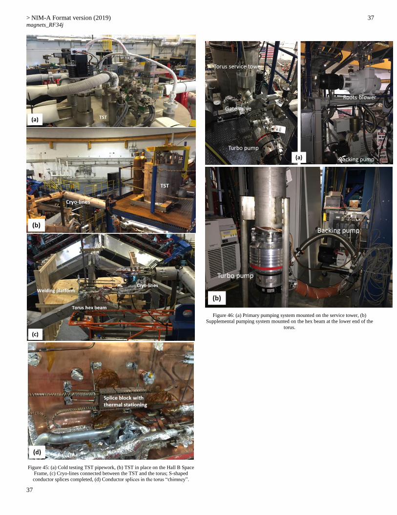
> NIM-A Format version (2019) magnets_RF34j
37
37
Figure 45: (a) Cold testing TST pipework, (b) TST in place on the Hall B Space Frame, (c) Cryo-lines connected between the TST and the torus; S-shaped
conductor splices completed, (d) Conductor splices in the torus “chimney”.
Figure 46: (a) Primary pumping system mounted on the service tower, (b)
Supplemental pumping system mounted on the hex beam at the lower end of the
torus.

> NIM-A Format version (2019) magnets_RF34j
38
38
Figure 47: (a) Screen shot of vacuum pumping control screen for the torus, (b)
Distribution can being delivered to Hall B, (c) Flexible copper jumpers
connecting the torus water-cooled leads to the magnet vapor-cooled leads.
Solenoid
The magnet was built by Everson-Tesla Inc. (ETI) and transported
by road to JLab using a purpose-built shipping cradle and
vibration isolation transport fixture (see Fig. 48). To assure safe
transport, several dummy runs between ETI and JLab were
carried out and data on the acceleration loads were collected.
These data were used for analysis of the magnet structure with
temporary shipping supports.
Figure 48: (a) Solenoid in shipping cradle and transport fixture at vendor, (b)
Solenoid arrival in at JLab.
Upon arrival at JLab, a visual inspection was completed along
with testing of the internal sensors and their wiring. The magnet
was then lifted onto its installation cart on the beamline in Hall B.
It was rough-aligned by the JLab survey and alignment team and
the temporary shipping braces were replaced with the final
supports and load cells. The Solenoid Service Tower (SST) built

> NIM-A Format version (2019) magnets_RF34j
39
39
by JLab was ready several months before the solenoid arrival, and
was already in Hall B and roughly positioned upon the space
frame above the beamline (see Fig. 49). With the solenoid on the
beamline, the SST was then aligned to the solenoid. The two
splices that connect the SST to the magnet were completed and
instrumented with voltage taps and temperature sensors before the
internal welding commenced. Pressure and leak tests followed,
similar to the torus. Finally, the multi-layer insulation blankets
were applied and the vacuum jacket was welded shut (see Fig.
50).
Figure 49: (a) The Solenoid Service Tower being lifted into place on the Hall B
Space Frame to await the arrival of the magnet, (b) Solenoid on its cart awaiting removal of axial support shipping fixtures and installation of axial support rods,
(c) One of eight axial support rods being fitted within a pocket that will then be
connected to a load cell, (d) Axial support load cell readings being checked for consistency prior to installation, (e) Solenoid in position on its “cart” with a
temporary wooden platform installed to allow welding of the service tower to the
magnet.
Figure 50: (a) Splices joining the magnet start and end leads to the vapor-cooled leads in the SST, (b) Splice block and cryogenic pipework wrapped in MLI, (c)
Service tower thermal shield welding completed, (d) Service tower – ready to
have its vacuum jacket closed up.
The magnet arrived from the vendors at the end of June 2017 and
was fully installed by early August 2017. The whole installation
process took less than 2 months using multiple teams working
around the clock. The final installed magnet is shown in Fig. 51.

> NIM-A Format version (2019) magnets_RF34j
40
40
Figure 51: (a) Ceramic break fitted to the top of the magnet vapor -cooled current leads – temporarily wrapped in paper, (b) Solenoid magnet installation
complete with “crow’s nest” service platform installed around the SST.
VII. COMMISSIONING AND TEST RESULTS
The vacuum spaces of both magnets were pumped down before
being cooled to operating temperature. Then tests were carried out
at predefined excitation currents to confirm that the overall
system response was as designed. All electromagnetic and
cryogenic parameters were monitored during the tests to validate
the cryogenic circuit design. Additionally, each magnet was
ramped to low currents to minimize its stored energy before a
controlled fast discharge was initiated. This allowed the JLab
team to check that all system protection mechanisms were
operating as designed, thereby mitigating any further risk when
the magnets were run at their full operating currents. The torus
magnet reached its full operating current of 3770 A without any
quenches in November 2016, while the solenoid reached its full
operating current of 2416 A in September 2017 with 5 quenches
in Coils 3 and 4 attributed to training quenches. The solenoid
retained all its quench training.
Each magnet has its own cryogenic service tower, which is fed
from a common cryogenic distribution box. The monitoring,
control, protection, power, vacuum, and cooling subsystems are
similar but independent for each magnet. Although the systems
are separate, a cryogenic “event” in one magnet can affect the
other and vice versa since both magnets share the same
distribution box [6].
Torus
Pump Down - Before the final vacuum pump down proceeded, all
the OOPS were properly set to allow for vacuum jacket
deflection. The pump down started gradually at about 2 psig/hr
for the first 7 hours to alleviate any coil-case “ballooning” effects
and to minimize any movement of the MLI. A roots blower
followed by turbo-molecular pumps were used to reduce the
pressure to about 10-4 Torr before initial cool down and several
backfills with gaseous nitrogen were used to assist with the
removal of water within the system. The pressure in the system
reached about 5x10⁻⁵ Torr after cool down started.
Purification -A process piping purification process using gaseous
nitrogen (GN2) and gaseous helium (GHe) was used to clean the
nitrogen and helium circuits. The nitrogen circuit only needed to
be free of water and flow purged with warm GN2. The helium
circuits needed to be free of water, as well as all other contaminate
gases.
The initial purification of the torus included purification of the
entire Hall B cryogenic system. This included all the warm gas
piping, ambient vaporizers, cryogenic transfer lines, distribution
box (DBX), U-tubes that interconnect the DBX to the 500-liter
helium buffer dewar, U-tubes that interconnect the DBX to the
torus, the Buffer Dewar, and the torus. There are 3 cold
connections at the End Station Refrigerator (ESR) that are used,
4K helium supply, 4K helium return, and LN2 supply. There are
two warm gas connections to the ESR, 300 K 4 atm helium and 1
atm 300 K return helium.
Cold-connection U-tubes at the ESR were not installed and the
warm connection valves were closed. Where possible each circuit
was purged with room temperature boil-off nitrogen gas for
several days to drive off moisture. The warm helium supply line
could not be purged this way because there is no vent on the ESR
end. It is also noted that care was taken not to pressurize the
helium circuits above 1 atm with nitrogen, to keep from
contaminating the operating ESR. The nitrogen circuits were then
pumped between 0.5 atm and 0.1 Torr three times and backfilled
with nitrogen. At this point the N2 circuits were considered clean.
The helium circuits were pumped and backfilled through the same
pressure range five times. Pumping and backfilling allowed
access to the small dead-end ranges of the circuits, such as the
pressure transducer and relief valve lines. After pumping and
backfilling the helium circuits, purging through the system was
done using clean helium from the ESR and sending it back to the
refrigerator helium recovery system. This recovery system has
nitrogen contamination monitors to verify the level of
contamination in the return gas. After the pump and backfills, the
return gas to the recovery system indicated that little to no
contamination was returned, thus our N2 purge, helium pump, and
backfills were deemed to have been successful and complete. A
similar process but on a much smaller scale was performed for the

> NIM-A Format version (2019) magnets_RF34j
41
41
solenoid.
Cool Down – The unique nature of the torus structure with a cold
hub and cold beams made it especially critical to minimize
temperature differences between the beams and the coils. Detailed
FEA calculations were done and showed that a maximum DT
(temperature gradient) of 50 K between them could be tolerated
during the cooling process at temperatures between 300 and 100
K for the 4 K mass. The independent nature of the LN2 shields did
not have this physical requirement. The piping of the supercritical
circuit is nearly 200 m long with most of it split equally between
tubes in the coils and re-coolers. Due to this long length, limited
flow at room temperature can be pushed through this circuit with
the 4-atm helium supplied to the hall at room temperature. To
achieve the required cool down time of 3 weeks, the re-coolers
were also designed to be used during the cool down process and
performed well.
The cool down of the torus was carried out using variable
temperature helium gas provided by the distribution box. Inside
the distribution box are two heat exchangers that cool one stream
of helium to 80 K. This 80 K helium was mixed with room
temperature helium to allow variable temperature gas to be fed to
the supercritical circuit and also the shell side of the re-coolers.
This then allowed the even cooling of all the coils and the hex
beams. During the cool down the maximum difference between
the average coil temperature and the average upstream hex beam
temperature was 12 K and it averaged about 10 K. For the
downstream beams vs. the coils, the maximum difference was 25
K at the beginning, but once the flows were balanced, it averaged
about 2 K. With these achieved values we were very safe
compared to our allowable difference of 50 K. For safety we had
the PLC programmed to shut off all cool down flow if the
differences ever exceeded the allowable maximum.
To gently cool the heat shield we took 80 K boil off from the LN2
pot in the distribution box and with an electrical heater in the U-
tube between it and the TST, heated the gas to provide a controlled
temperature gas to the shield. Again this was interlocked to turn
off the heater and the flow if the maximum difference between
any of the six coil shield outlets and the shield supply reached 60
K.
From room temperature to about 100 K the cool down rate of the
torus was 0.5-0.7 K/hr. The cool down time from 300 K to about
4 K for the torus was calculated to be about 14 days assuming a
maximum temperature differential across the cold mass of 30 K
and a helium flow rate of 7 g/s. In reality, the cool down took
longer and was carried out in several steps. During the cool down
process (at about an average CCM temperature of 209 K), it was
noted (via observation of strain gauge readings on the supports)
that the four torus vertical supports were apparently bending. This
necessitated a slow-down in the cooling process (to about 170 K)
and finally a temporary halt while measurements and strain gauge
calibrations were checked. It was discovered that although some
of the strain gauges were not being adequately temperature-
compensated, the vertical supports were indeed experiencing
some level of bending. A risk review was convened to plan the
path forward and four options were considered – which included
a “worst” case option that required a warm-up to room
temperature to repair the vertical supports by cutting into the
vacuum jacket. A spare vertical support was tested at liquid-
nitrogen temperature and was demonstrated to have a more than
adequate strength safety factor under bending (see Fig. 52). It was
thus experimentally determined that it was safe to continue with
the torus cool down, which was then resumed and the torus
achieved its helium operating temperature of 4.5 K without any
further issues.
Figure 52: (a) Bend testing a spare torus vertical support.
Steady State Cooling - The upstream (US) cold hex beams contain
the cryogenic and electrical connections (splices) between coils,
as well as the re-cooler heat exchangers. The re-coolers contain
liquid helium and are connected by large tubes to the helium
reservoir at 1.3 atm located within the TST. Two small tubes
originate at the bottom of the TST and run through the three re-
coolers, exiting at the bottom of the re-cooler outer shell. Since
the liquid in the small tube is denser than the heated fluid in the
re-cooler’s outer shell, a thermo-siphon is used to exchange the
cooler reservoir liquid with the shell side fluid. The 1.3 atm.
liquid helium cools the 3.0-atm helium before entering each coil.

> NIM-A Format version (2019) magnets_RF34j
42
42
Figure 53: Simplified flow diagram of the CLAS12 torus helium and nitrogen cooling circuits.
The cooling scheme (see Fig. 53) consists of three separate flow
circuits as follows:
a) 1.3 atm helium circuit – The LHe reservoir (shown in light
blue) within the TST, is filled with liquid helium. LHe then
flows down through the re-coolers to the blue dot shown in
the figure. Thermal-siphon flow returns helium back up
through the re-cooler outer shells and via the upstream hex
beams.
b) Supercritical helium at 3.0 atm – This circuit (shown in dark
blue) passes through a re-cooler coil within the helium
reservoir in the TST. It then flows through six coil and re-
cooler units and also through tubes used to cool the
downstream cold hex beams. Finally, it flows through a heat
exchanger coil in the TST helium reservoir before flowing
through the Joule-Thompson valve that is used to fill the TST
reservoir.
c) The 1.3 atm LN2 circuit – This circuit (shown in green) also
uses the thermo-siphon effect. It has one main feed that
separates into 8-parallel branches that keep each thermal
radiation shield at ~80 K (see Fig. 54). Of the 8 branches, 2
branches cool the downstream hex beam thermal radiation
shields, while 6 cool the coil thermal radiation shields.
Figure 54: Steady state temperature distribution across one of the thermal shields.

> NIM-A Format version (2019) magnets_RF34j
43
43
Torus process safety
In Ref. [37] the worst-case scenario was considered of having a
loss of vacuum (LOV) and a simultaneous magnet quench, and
this work assisted in the development of the operational protocol
for the cryogenic process. Pressure relief valves protect the piping
systems from over-pressure during an LOV, quench, or fast dump.
Five relief valves are used for the 3.0-atm cooling circuit. Three
valves are located on the Hex Ring Vacuum Jackets and are set to
vent at 5.3 atm; they are located strategically in the path of the
CCMs and re-coolers. The remaining two valves are located on
the TST and are set to vent at 4.6 atm. A check valve in the supply
U-tube prevents any back pressure into the distribution box in the
event of a fast dump. The 1.3-atm circuit is protected by a 2.7-atm
relief valve located on the TST.
The highest system pressure for this circuit will occur during a
LOV and magnet quench at the farthest point from the relief valve
in the re-cooler piping. The LOV will impart a major proportion
of the energy to the 1.3-atm circuit while a magnet quench imparts
a smaller proportion of energy; first to the 3.0-atm helium flow
and then into the 1.3-atm system via the re-coolers.
However, the highest system pressure for the 3.0-atm circuit
(during a relief event) occurs at a location buried within the coils
and re-coolers, at a point in the circuit between the relief valves,
where flow may go both ways. Using a simple model to estimate
the system pressure rise (assuming all energy generated is
transferred to the helium), the estimated pressure rise (during a
fast dump) is shown in Fig. 55. It is apparent that if all the energy
from the 3000 A fast dump was transferred to the helium, the
design pressure of 20.0 atm of the system would be exceeded.
However, using calculations from a more detailed model, it was
demonstrated that the 20.0-atm pressure rating of the pipes would
not be exceeded in the torus circuit due to the distribution of
energy throughout the entire system. Our commissioning tests
have since validated the results from this analysis.
Figure 55: Estimate of torus helium circuit pressure with time at increasing operating currents based on the simple model.
System Energy Balance Modelling – As part of the
commissioning process, system heat loads were estimated for
each of the energization states. A Detailed Predictive Model
(DPM), based on the Wilson model, was used to calculate the
heat loads [16]. The DPM assumes that a fast dump would
release all of the magnet’s stored energy (see Fig. 56). The
DPM predicted that the torus could be operated safely, up to the
nominal operating current of 3770 A, for all energization states
and fault scenarios.
After energization and initial testing at low currents, the magnet
was ramped up to 3000 A and parked. An unexpected fast dump
was triggered by the PLC comparator controls during this period.
The team took advantage of this unexpected event and having
reviewed this 3000 A fast dump data, the results clearly indicated
that the magnet was safe to also fast dump from 3770 A. These
results were also used to calibrate and validate the Detailed
Predictive Model.
A maximum average temperature for all the CCMs was recorded
as being <40 K during the 3000 A fast dump. The tests and
analyses perfomed validated the pressure relief and the torus
cryogenic system design thus confirming that the system was
indeed safe.

> NIM-A Format version (2019) magnets_RF34j
44
44
Figure 56: (a) Flow diagram representing the extraction of stored energy in the
magnet during a fast dump or in the event of a quench, (b) Plots for the energy
calculated based on measured data during fast dump events at various operating currents up to 1750 A (approximated with a polynomial fit to the measured data
points).
Solenoid Pump Down and Purification
The pump down of the solenoid was much faster and easier
because the magnet has much less surface area, an overall smaller
size, and better conductance between the turbo pump and the
magnet. Purification was done similarly to the torus using a GN2
purge for several days, followed by 5 pump and backfills, then
flowing to the purifiers while monitoring the contamination level.
Solenoid Cooling
This five-coil magnet is also conduction cooled by 4.5 K helium,
but unlike the torus coils, the heat is directly transferred to liquid
instead of supercritical gas. The cool down system for the
solenoid is the same one as for the torus and was used while the
torus was at 4.5 K. Similar interlocks and controls were used to
assure safe cool down. The magnet’s liquid helium cooling
channel is located between the two main inner coils and runs
around the inner diameter of the bobbin. The thermal shields are
cooled using the boil-off from the magnet LHe reservoir. The
magnet is held at its operating temperature by conduction cooling
via a thermo-siphon helium circuit from the magnet reservoir (see
Fig. 57). Adequate instrumentation with redundancy is provided
to monitor and control the magnet cool down and steady state
operation.
Pre-commissioning checks on all subsystems, controls, and
instrumentation were carried out for each magnet prior to starting
the commissioning process. The torus and solenoid were cooled
in 2-steps. Variable temperature gas was used to cool from 300
K-100 K, followed by LHe to 4.5 K.
Figure 57: Simplified cooling circuit schematic for the solenoid.
The inlet temperature to the coils, average coil, and outlet
temperature were monitored. The maximum cooling rate was
limited to 2 K/hr (see Fig. 58).
The experience with magnet cool down for both systems can be
summarized as follows:
• Total time = 43 days (torus), 23 days (solenoid);
• Cooling time =19 days (torus), 23 days (solenoid);
• Helium temperature controlled at 45 K below the
maximum metal temperature for the torus and between
35 K and 60 K below maximum metal temperature for
the solenoid;
• The maximum allowed metal temperature differences
for the torus was limited to 50 K, while for the solenoid
it was 46 K. In practice the maximum temperature
differences were controlled to about 25 K for the torus
and about 40 K for the solenoid;
• Cool down helium flow rate for the torus was 6-7 g/s and
5-6 g/s for the solenoid.
At steady state the solenoid magnet itself requires only 0.4 g/s of
liquid helium for its cooling. This flow was measured directly
using a room temperature flow meter. This flow rate does not
include the amount of flow needed for the VCLs, the lead
reservoir, or the primary supply and return U-tubes.

> NIM-A Format version (2019) magnets_RF34j
45
45
Figure 58: Torus and solenoid cool down (torus cool down: Start-August 12, 2016; Complete-September 22, 2016 and solenoid cool down: Start-August 5, 2017;
Complete-September 7, 2017).
During commissioning, [38] both the torus and solenoid were
energized in steps to full operating current. Predetermined fast
dumps were also carried out to check on the instrumentation and
proper functioning of the magnet protection. Typical temperature
increases of the torus and solenoid magnet coils during ramp up
and down to and from full operating current are shown in Fig. 59
and are a result of eddy current heating within the coils
themselves. The temperature increases were modest (no higher
than about 0.3 K) and well within the calculated 1.2 to 1.5 K
temperature margin of the coils, but were nonetheless used to
modify the ramp rates for both magnets to minimize eddy current
heating.

> NIM-A Format version (2019) magnets_RF34j
46
46
Figure 59: (a) Torus CCM B temperature rise during a ramp to 150 A at 2 A/s due to eddy current heating, (b) A typical plot of temperature rise in the solenoid coils
during normal ramp-up and down.
As part of the commissioning process, several fast dumps were
carried out at low stored energies in the magnet and were found
to match well with the predictive models. All tests carried out
indicated that both magnets had more than adequate safety
margins with regards to pressure relief of subsystems and coil
temperature rise. The coil temperatures recorded during a fast
dump event, 3000 A (torus) and 2047 A (solenoid), are shown in
Fig. 60.

> NIM-A Format version (2019) magnets_RF34j
47
47
Figure 60: Coil temperature rise - during a fast dump (a) Torus, (b) Solenoid.
There is a level of electromagnetic coupling between the torus and
solenoid coils [25]. As the torus is ramped to full field (3770 A)
Fig. 61a shows the change in the OOPS load cell readings for the
torus CCM-A. This change in force is small and due to a slight
mechanical asymmetry in the spacing between the 6 coils. The
solenoid radial and axial load cell readings also change during a
ramp up of the solenoid to its full operating current of 2416 A,
followed by a controlled ramp down to zero amps (see Fig. 61b).
Based on the defined load cell limits, the force experienced by the
torus coil within its vacuum jacket during energization is not high
enough to initiate a controlled ramp down of the magnet. This
behavior is demonstrated by all 6 torus coils with only minor
variations depending on the location of the coil on the magnet due
to gravity-loading. This behavior was also noted to be extremely
repeatable following many cycles of magnet energization and de-
energization. For the solenoid, it is encouraging to note that all
forces revert back to almost the original values after de-
energization, illustrating linear response of the coil support
structures. It has also been shown from subsequent runs that this
process is very repeatable.
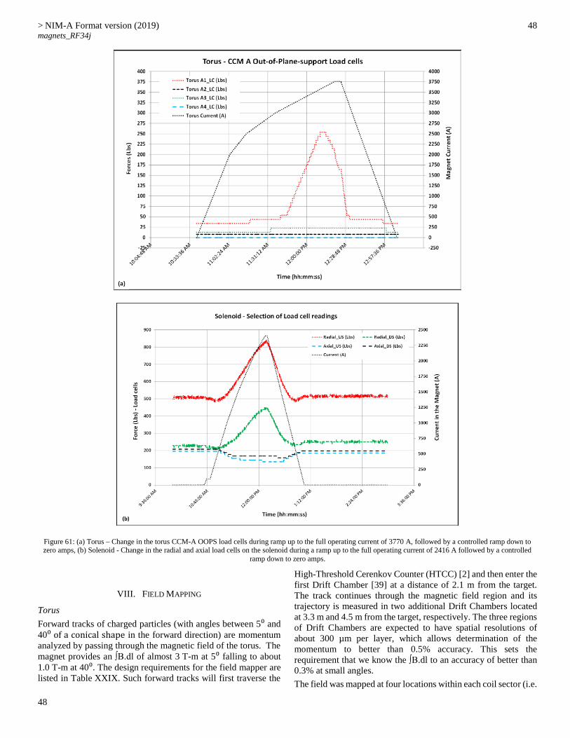
> NIM-A Format version (2019) magnets_RF34j
48
48
Figure 61: (a) Torus – Change in the torus CCM-A OOPS load cells during ramp up to the full operating current of 3770 A, followed by a controlled ramp down to zero amps, (b) Solenoid - Change in the radial and axial load cells on the solenoid during a ramp up to the full operating current of 2416 A followed by a controlled
ramp down to zero amps.
VIII. FIELD MAPPING
Torus
Forward tracks of charged particles (with angles between 5⁰ and
40⁰ of a conical shape in the forward direction) are momentum
analyzed by passing through the magnetic field of the torus. The
magnet provides an ∫B.dl of almost 3 T-m at 5⁰ falling to about
1.0 T-m at 40⁰. The design requirements for the field mapper are
listed in Table XXIX. Such forward tracks will first traverse the
High-Threshold Cerenkov Counter (HTCC) [2] and then enter the
first Drift Chamber [39] at a distance of 2.1 m from the target.
The track continues through the magnetic field region and its
trajectory is measured in two additional Drift Chambers located
at 3.3 m and 4.5 m from the target, respectively. The three regions
of Drift Chambers are expected to have spatial resolutions of
about 300 µm per layer, which allows determination of the
momentum to better than 0.5% accuracy. This sets the
requirement that we know the ∫B.dl to an accuracy of better than
0.3% at small angles.
The field was mapped at four locations within each coil sector (i.e.

> NIM-A Format version (2019) magnets_RF34j
49
49
between coils) – one measurement at a radius of 30 cm and three
measurements at a radius of 46.5 cm but at different Φ angles, as
well as within the bore. Multiple measurements were made at
each of these locations along the z-axis – i.e. in the direction of
the beamline. The mapping equipment consisted of a digital
voltmeter, 2-in diameter carbon tube referenced to survey points,
three single axis calibrated Hall probes (one for each of the x, y,
and z axes) positioned in a cylindrical block of Delrin® spaced 5
cm apart in the z-direction, and a control system (for motion, data-
recording, and interlocks) [40]. A commercially available Group
3 MPT-141 series of transverse Hall probes with a DTM-151
Tesla-meter was used for the field measurement. The
measurement accuracy of the probes and meter at 250C, with a
shielded cable length of 300 mm x ø6.5 mm, is ± 0.01% of the full
scale reading. The Hall probes are temperature compensated and
were also surveyed to a positional accuracy of 0.040 mm within
the Hall probe holder. Precisely machined plates were attached to
the upstream and downstream ends of the torus with matching
through holes used to locate long lengths of carbon fiber tubes.
The Hall probe holder was moved along the z-axis inside the
carbon fiber tubes using a linear slide and stepper motor while
magnetic field data was recorded at each measurement point [41].
The magnetic field measurement fixtures with locations are
represented in Fig. 62.
TABLE XXIX
TORUS MAPPER SPECIFICATIONS SUMMARY
Field & Position Accuracy
Bø 0.1 %
Br 1 %
Bz 1 % Radial ±0.1 mm
Azimuthal ±0.1 mm
z-position ±0.5 mm
Figure 62: Torus magnetic field measurement locations – 4 locations in each sector and 7 locations in the bore (1 in the center and 6 spaced 60o apart at a radius of
2.5 cm) – field measured at 5 cm increments in z (along the beam axis) along with the torus magnetic field measurement locations (HA, HB, HC, and HD are within each
sector, i.e. between coils).
The magnet field map was created using the original
electromagnetic model. This model included thermal contraction
effects but was based on a nominal coil design that did not include
the real effects of dog-boning, the shimming, or compaction in the
areas of tight bend radii.
As stated earlier in the coil fabrication discussion, spacers were
added prior to the first potting to allow more accurate and
consistent conductor positioning especially closer to the hub. Data
from the optical surveys allowed better knowledge of the actual
positioning of conductors within the coil (see Fig. 63). This was
then used to create a new electromagnetic model of the coil. That
model was compared with data from the field map.
46.5 cm Radius
HD HC HB HA

> NIM-A Format version (2019) magnets_RF34j
50
50
Figure 63: A close-up view of a coil near one bend after the 1st epoxy
impregnation to allow data capture of the location of each turn in the coil.
Torus Design Model and Analysis: The torus model coil design
was carried out using the commercial OPERA-TOSCA software
from Cobham and field maps were produced as the baseline for
the magnet field measurement (see Fig. 64). All design models
were analyzed utilizing cold (contracted) dimensions with the
magnet at its full operating current of 3770 A. The mapping of the
field was carried out at 3000 A and the model data was scaled
from 3770 A to 3000 A. The measured results obtained were
significantly different from the original model data. The results
were analyzed to calculate the “distortion field” – i.e. the
difference between the measured and calculated field values using
a chi-squared function (χ2) that compared the measured data
deviation from the nominal modeled field data [42].
Figure 64: Single pancake of one torus coil (a) Coil survey points from 17 sections in the coil, (b) The design model prepared in Opera® with 17 sections and further
discrete subsections, (c) Magnetic flux density variation near and though the coil case of the torus for a simplified version of the conductor (assuming one large contiguous conductor block) and a refined discrete model where the two coil pancakes are modeled individually with current flow only within the superconducting
Rutherford cable.

> NIM-A Format version (2019) magnets_RF34j
51
51
The magnetic field modeling was improved via a 4-stage process:
Stage I: Symmetric “Block Model” - Symmetric ideal coil
model (nominal with cold coil dimension, 2 pancake coils
simply modeled as one large contiguous block);
Stage II: Asymmetric Block Model- Block model combined
with relocated coil position;
Stage III: Symmetric “Discrete Model” - Symmetric coil
model with surveyed conductor location (with cold coil
dimension), with 2-individual pancakes; Current in individual
pancakes considered;
Stage IV: Asymmetric Discrete Model – coil model with
surveyed conductor locations combined with relocated coil
positions.
The absolute field data plot is presented in Fig. 65. The plots
show that the variation in the magnetic field distribution is about
+4.96 % for the block model and about -0.9 % for the discrete
model in a sector when compared to the measurements.
Figure 65: Magnetic flux density distribution (a) sector 1 - HA (b) sector 1 – HD,
between block model – symmetric, asymmetric, and “discrete model” compared
with measured data.
Summary of findings - At distances far from the hub and coils, all
models accurately represent the field, but since the detector needs
a model that accurately represents the field at small angles (near
the hub), as well as over a large azimuthal angle in (from one
coil to the next), only the discrete model should be used. Work
continues to confirm that the ∫B.dl is known better than 0.3 %
accuracy at small angles.
a. The percentage variations cited are for one-to-one
comparisons using two-dimensional percentage analysis
(block model and discrete model) and the averages were
calculated separately based on χ2.
b. Average inner (30 cm radial position) measurements indicate
a 0.5% deviation from the measured data.
c. Average outer (46.5 cm radial position) measurements
indicate a 0.05% deviation from the measured data.
d. Fluctuations in the inner measurement deviations are
consistent and attributed to the effect of a 1.5 mm change to
the outer radius of the coil shape.
An additional benefit of adopting the detailed model was to allow
us to re-calculate the peak field on the torus coil; the peak field
increased by just over 1% from 3.58 T (using a simple model) to
3.62 T (using the detailed model) confirming that the load lines
shown earlier are still valid.
Solenoid
Measurements were carried out to establish the following:
a. To quantify the magnetic length of the solenoid;
b. To verify the high homogeneity region (over a 25 mm
diameter x 40 mm length cylinder) at the center of the
magnet;
c. To measure the magnetic fringe fields at the specified
detector locations.
The torus mapper was adapted for the field mapping of the
solenoid magnet. The external fixture holds the 2-in diameter
carbon fiber tubes at precise x-y positions and uses a linear stage
drive to move the probes in the z-direction. The Hall probe holder
was placed within the carbon-tube in order to zero the z-position
of the linear slide before the start of the z-map for the particular
location in question. The z-map consisted of driving the Hall
probe holder in 5 cm steps along z and pausing for 5 s for the Hall
probes to settle before recording the probe data for each of the 3-
sensors. Figure 66 shows the typical arrangement for the solenoid
magnet field measurement along the bore and off-center
locations.

> NIM-A Format version (2019) magnets_RF34j
52
52
Figure 66: Typical arrangement for the solenoid magnet field measurement along the bore and off-center locations.
During commissioning of the solenoid magnet, the field mapping
was carried out at different operating currents in order to confirm
the design specifications. Field mapping was performed along the
z direction at 9 locations; one at the geometrical center of the
magnet and at 8o to 45o positions at a radius of 12.5 mm. The
magnetic field was also measured along the z-axis at a 30 cm
radius at a 60o angle from horizontal. To verify the field
homogeneity of the magnet, measurements were taken at the
center of the magnet at 10 mm intervals along the z-axis.
The magnet length, L, defined as B0-1.∫B.dl was measured to be
1.41 m. The measured homogeneity, ΔB/B0, over a 40-mm-long
x ϕ25 mm cylinder was better than 300 ppm and satisfied the
present physics experimental requirements. To achieve the
desired 100 ppm for planned future polarized target experiments,
the JLab Target Group is intending to design and install small
superconducting corrector coils that will be positioned directly
over the target. Fringe field measurements at the detector
locations were carried out using a hand-held field probe and a
template board to help position the probe.
The central field of the solenoid is 5 T, but the Hall sensors were
calibrated only to 3 T. Therefore, field mapping was limited to 3
T (corresponding to an operating current of 1450 A). The central
field at higher currents was verified using an NMR probe.
Another limitation of this mapper was the extent to which it could
map in the z-direction, as the linear stage was limited to about 1.9
m. The measured field over this length was compared with the
model data to find the effective length of the magnet. The field
mapping results are summarized in Table XXX.
TABLE XXX
SOLENOID – REQUIRED AND MEASURED PERFORMANCE PARAMETERS
Performance Parameter Broad Specification Actual Measured
B0 5T 5.0 T
L= B0-1.∫B.dl (B0 field at the
center (0,0,0) of solenoid) L = 1 to 1.4 m 1.41 m
Field uniformity in target area
ΔB/B0 < 10-4 in cylinder 25
mm diameter x 40 mm
length (100 ppm)
318 ppm
(to be improved using superconducting
corrector coils
around the target)
Field at HTCC PMT
locations
B < 35 G - for the four
HTCC PMT locations B = 6-22 G
Field at CTOF PMT locations
B < 1200 G - for the two CTOF PMT locations
B = 43-1041 G
The mapped data was compared with the as-wound cold-
contracted (4.5 K) coil model data. There is still a slight
discrepancy between the two data sets for the central field and the
field at a radius of 30 cm. The model uses 208 block conductors,
as follows - each layer for the inner and intermediate coils is
assumed to be one block conductor, while each layer for the shield
coil has been split into 2 block conductors:
2*42 layers for inner coils (84 block conductors);
2*46 layers for intermediate coils (92 block conductors);
The shield coil has 16 layers, but each layer was divided into 2
block conductors (32 block conductors).
The discrepancy between the model and measured data could be
attributed to coil positioning errors or coil movement during
energization. The theoretical model is being improved to better
match the mapped data. One of these improvements involves
moving the inner and intermediate coils radially or axially - these
results are shown in Figs. 67 - 70. Figure 67 shows the comparison
of model, mapped and data produced with an inner coil axial
movement; Figure 67a shows the field in the central region while
Fig. 67b shows the off-axis field data. It is clear from Fig. 67 that
an inner coil axial movement alone is not sufficient to reproduce
the mapped data. Figure 68 shows the same data with a radial
movement of the inner coils and again the mapped data and data
modeled with this radial change do not match. Figures 69 and 70
show similar data with the middle (intermediate) coil moved
axially and radially. It is clear from the manipulation of the
modeled data that a single coil movement alone cannot fully
explain the variation between the modeled and mapped data. A
combination of inner and middle coil movement together with a
movement variation in the shield coil might result in a better
match between model and mapped data. This work is still in
progress.
Guide plate to position the carbon fiber tube with hall sensor in the magnet along the bore axis
(z-axis)
Carbon fiber tube with hall sensor
external fixture to hold 2” diameter carbon fiber tubes
Support fixture to hold and position the guide plate in the
magnet bore
(a) (b)

> NIM-A Format version (2019) magnets_RF34j
53
53
Figure 67: (a) Comparison of model and mapped data at r=0 cm with the inner coils moved axially.
.
Figure 67: (b) Comparison of model and mapped axial data at r=30 cm with the inner coils moved axially.
Figure 68: (a) Comparison of model and mapped data at r=0 cm with the inner coils moved radially.

> NIM-A Format version (2019) magnets_RF34j
54
54
Figure 68: (b) Comparison of model and mapped axial data at r=30 cm with the inner coils moved radially.
.
Figure 69: (a) Comparison of model and mapped data at r=0 cm with the middle (intermediate) coils moved axially.
Figure 69: (b) Comparison of model and mapped axial field data at r=30 cm with the middle (intermediate) coils moved axially.

> NIM-A Format version (2019) magnets_RF34j
55
55
Figure 70: (a) Comparison of model and mapped data at r=0 cm with the middle (intermediate) coils moved radially.
Figure 70: (b) Comparison of model and mapped radial field data at r=30 cm with the middle (intermediate) coils moved axially.
Operational Experience
Both the torus and the solenoid have performed very well since
being commissioned in 2016 and 2017, respectively [38].
However, between September 2017 and February 2019 there were
a total of 15 fast dumps of the solenoid – i.e. the dump switch
would open and the magnet would run down through its dump
resistor. One fast dump was attributed to a malfunctioning
mechanical switch on the voltage tap diagnostic panel and a
second being due to an incorrectly set quench detection threshold
setting. The remaining 13 dumps were initially incorrectly
identified as being due to magnet coil voltages exceeding their set
quench detection thresholds. Several causes were postulated:
The voltage thresholds apparently being exceeded were those
associated with the vapor-cooled leads. Thus initial thoughts
were that a resistance was developing across these leads
perhaps due to a deteriorating joint. However, examination
of all the data collected thus far indicated that all of the joints
were good and none displayed any deviation from normal
expected resistances for all operating currents and varying
helium levels within the lead reservoir. Movements of the
leads producing induced voltages were also ruled out due to
the robust mechanical support of the leads within the
reservoir and the extremely low magnetic field in that region.
We eliminated any potential issues with our fast data
acquisition and quench detector electronics by carrying out a
series of voltage injection tests. We also reviewed and
improved some of the grounding for our wiring and
electronics.
Investigation of the way in which we were recording and
“packaging” the voltage tap data via our fast data acquisition
electronics indicated that our data had unintended offsets in the
time stamps - hence the false voltage tap triggers that we believed
caused the fast dumps. This data packaging and translation has
now been improved.
Additional diagnostics and relays were fitted to the power supply
and dump switch so we could time stamp when the dump switch

> NIM-A Format version (2019) magnets_RF34j
56
56
opened with respect to the triggering of the quench detection
units. Examination of the time stamps of subsequent solenoid fast
dumps clearly indicated that the trips were originating from the
power supply interlocks, which unfortunately had been masked
by the false voltage trip data. A more detailed investigation
revealed a strong correlation with temporary reductions in cooling
water flow to the magnet power supply. This phenomenon was
traced to the low conductivity water (LCW) expansion tank,
(which is also shared by two other experimental halls), being
topped up at intervals thus affecting the regulation of water flow
to the hall and thus the magnet power supply. We made several
improvements to the overall system including adding more
margin for the flow switches within the power supply itself, using
larger diameter pipework from the water manifold to the power
supply, and most importantly, improving the regulation of the
expansion tank and thus the flow of water to our experimental
hall.
A re-examination of the data associated with the 13 fast dumps
revealed that indeed there was a correlation with a reduction of
the LCW to the hall and the power supply. To date, the solenoid
has not suffered from any additional fast dumps and both magnets
continue to operate within all normal expected parameters.
Summary
As with any typical project, the key drivers were technical
reliability, schedule, and cost. These drivers encouraged the team
to adopt and extensively use the Failure Modes and Effects
Analysis (FMEA) methodology for both magnets from design
through to installation and commissioning. Regular reviews such
as the Magnet Advisory Group reviews, JLab Director’s Reviews,
and U.S. Department of Energy Office of Project Assessment
Reviews, provided a clear focus and boundaries for the JLab
project team. The skills, resourcefulness, and outstanding work
ethic of the members of the 12 GeV Magnet Task Force, coupled
with the support and commitment of other groups and
departments within the laboratory, enabled the project team to
flex its planning, management, and execution strategies to
overcome all manner of obstacles, including sub-standard potting
of torus coils, vendor quality issues on the distribution box, cool
down issues involving vertical supports for the torus, and the later
than expected delivery of the solenoid to name the key ones.
Ultimately both the superconducting torus and solenoid magnets
developed and constructed to be used for the new CLAS12
spectrometer have met the required system specifications that will
enable the full physics program to be carried out.
Acknowledgements
The authors would like to acknowledge the contributions and
support from all Hall B staff, Hall D staff, the Engineering
Division, Magnet Measurement Group, DC Power Group,
Cryogenics Group, Detector Support Group, Target Group, Fast
Electronics Group, Engineering Support Services, SRF,
Procurement Team, Travel, ESH&Q, Human Resources, Payroll,
Planning, Finance, Information and Technology (IT), JLab
management and, in particular, the 12 GeV leadership team, the
12 GeV Project Support Staff and the technicians at JLab. The
authors would also like to thank reviewers, to name a few in
particular, S. Prestemon (LBNL), B. Flora (FNAL), and H. ten
Kate (CERN). Thanks are also due to Fermilab for the fabrication
of the torus coils and the key vendors, Advanced Engineering
Systems (conductor soldering), Tesla Engineering Limited
(Solenoid design), Everson Tesla Inc. (solenoid build), Meyer
Tool (distribution box), and the University of Durham (conductor
splice testing). A special mention is also due to the following
individuals who have contributed to the success of this project:
M. Anerella, J. Ballard, K. Bruhwel, G. Cheng, J. Creel, J.
Fischer, J. Gomez, S. Gregory, V. Hagen-Gates, D. Hampshire,
L. Harwood, V. Lagerquist, A Makarov, M. Marchlik, F. Martin,
W. Oren, S. Plate, L. Quettier, S. Radovic, B. Reinhart, P. Rossi,
E. Salpietro, W. Schneider, K. Smith, E. Stallworth, M. Stirbet, J.
Szal, C. Wiggins, T. Willard, and M. Zarecky.
This material is based upon work supported by the U.S.
Department of Energy, Office of Science, and Office of Nuclear
Physics under contract DE-AC05-06OR23177. The U.S.
Government retains a non-exclusive, paid-up, irrevocable, world-
wide license to publish or reproduce the published form of this
manuscript, or allow others to do so, for United States
Government purposes.
REFERENCES
1. V.D. Burkert et al., “The CLAS12 Spectrometer at Jefferson
Laboratory”, to be published in Nucl. Inst. and Meth. A,
(2020). (see this issue)
2. Y.G. Sharabian et al., “The CLAS12 High Threshold
Cherenkov Counter”, to be published in Nucl. Inst. and Meth.
A, (2020). (see this issue)
3. D. S. Carman et al., “The CLAS12 Central Time-of-Flight
System”, to be published in Nucl. Inst. and Meth. A, (2020).
(see this issue)
4. Luongo, C., Ballard, J., Biallas, G., Elouadrhiri, L., Fair, R.,
Ghoshal, P., et al., “The CLAS12 Torus Detector Magnet at
Jefferson Lab”, IEEE Transactions on Applied
Superconductivity, V26 (4), 2016, DOI - 10.1109/
TASC.2015.2510336.
5. Krave, S., Velev, G., Makarov, A., Nobrega, F., Kiemschies,
O., Robotham, B., et al., “Overview of Torus magnet coil
production at Fermilab for the Jefferson Lab 12-GeV Hall B
upgrade”, IEEE Transactions on Applied Superconductivity,
V26 (4), 2016, DOI 10.1109/TASC.2016.2533264.
6. Ghoshal, P. K., Bachimanchi, R., Fair, R. J., Kashy, D.,
Rajput-Ghoshal, R., Hogan, J., Sandoval, N., Young,
G., “Instrumentation and Control Selection for the 12 GeV
Hall-B Magnets at Jefferson Lab”, Supercon. Sci. and Tech.,
V31 (9), 095007, 2018, DOI: 10.1088/1361-6668/aad277.
7. Fair, R. J. & Young, G. R., “Superconducting Magnets for
the 12 GeV Upgrade at Jefferson Laboratory”, IEEE
Transactions on Applied Superconductivity, V25 (3), 2015,
DOI - 10.1109/TASC.2014.2365737.
8. Ghoshal, P. K., Biallas, G., Fair, R. J., Rajput-Ghoshal, R.,
Schneider, W., Legg, R., et al., “FMEA on the
Superconducting Torus for the Jefferson Lab 12GeV
Accelerator Upgrade”, IEEE Transactions on Applied

> NIM-A Format version (2019) magnets_RF34j
57
57
Superconductivity, V25 (3), 4901005, 2015, DOI -
10.1109/TASC.2015.2388591.
9. Ghoshal, P., Pastor, O., Kashy, D., Schneider, W., Wiseman,
M., Zarecky, M., et al., “Electromagnetic and Mechanical
Analysis of the Coil Structure for the CLAS12 Torus for 12
GeV Upgrade”, IEEE Transactions on Applied
Superconductivity, V25(3), 4500705, 2015, DOI
10.1109/TASC.2014.2382604.
10. de Hoog, F. R., Cozijnsen, M., Yuen, W. Y. D. and Huynh,
H. N., “Predicting Winding Stresses for Wound Coils of
Linear Orthotropic material”, in Proc. Instrumentation Mech.
Engineers, Part C, J. Mechanical Engineering Science, 218
(C1), 13–25, 2004.
11. Li, S and Cao, J., “A Hybrid Approach for Qualifying the
Winding Process and Material Effects on Sheet Coil
Deformation”, J. Engineering Materials and Technology,
V126, pp. 303-313, July 2004.
12. Knight, C. E., “Residual Stress and Strength Loss in
Filament-wound Composites”, Composite Materials: Testing
and Design (Eighth Conference), Editor: J. D. Whitcomb,
ASTM, 1988.
13. Arp, V., “Stresses in Superconducting Magnets”, Journal of
Applied Physics, V48, No. 5, pp. 2026-2036, May 1977
14. Pojer, M., Devred, A & Scandale, W., “A Finite Element
Model for Mechanical Analysis of LHC Main Dipole Magnet
Coils”, LHC Project Report 1001, Applied Superconductivity
Conference (ASC 2006), 2006.
15. P. K. Ghoshal, R. J. Fair, D. Hampshire, V. Hagen-Gates, D.
Kashy, R. Legg, R. Rajput-Ghoshal, Y. Tsui, “Design and
Evaluation of joint resistance in SSC Rutherford type cable
splices for Torus magnet for the Jefferson Lab 12 GeV
Upgrade,” IEEE Transactions on Applied Superconductivity,
2016; V26(4), DOI - 10.1109/TASC.2016. 2517922
16. M. N. Wilson, “Superconducting magnets,” Oxford
University Press, UK, 1983
17. V. S. Kashikhin, L. Elouadrhiri, P. K. Ghoshal, D. Kashy, A.
Makarov, O. Pastor, et al., “Torus CLAS12-Superconducting
Magnet Quench Analysis,” - IEEE Trans on Appl.
Superconductivity, Vol 24. No. 3, June 2014 (DOI
10.1109/TASC.2014.2299531).
18. P K Ghoshal, R. J. Fair, R. Rajput-Ghoshal, “Torus
Analytical Quench analysis - Single coil quench analysis Hall
B Torus”, JLab Internal Document # B00000401-A012
(April 23, 2013)
19. OPERA-3D User Guide, Version 18R2, Cobham Technical
Services, Network House, Langford Locks, Kidlington,
U.K., May 2016.
20. Pastor, O., Willard, T., Ghoshal, P., Kashy, D., Wiseman, M.,
Kashikhin, V., Young, G., Elouadrhiri, L., & Rode, C.,
“Structural Analysis of Thermal Shields During a Quench of
a Torus Magnet for the 12 GeV Upgrade”, IEEE
Transactions on Applied Superconductivity, V25 (3), 2015,
DOI-10.1109/TASC. 2014.2371820.
21. Fazilleau, P., Ball, J., Herview, B., & Pes, C., “CLAS 12
Solenoid Magnet Technical Design Report”, Centre de
Saclay, A-CRYOM-02-07-01-01-RT05.
22. M.A. Antonioli et al., “The CLAS12 Silicon Vertex
Tracker”, to be published in Nucl. Inst. and Meth. A, (2020).
(see this issue)
23. P. Chatagnon et al., “The CLAS12 Central Neutron
Detector”, to be published in Nucl. Inst. and Meth. A, (2020).
(see this issue)
24. F. Bossu et al., “The CLAS12 Micromegas Vertex Tracker”,
to be published in Nucl. Inst. and Meth. A, (2020). (see this
issue)
25. Rajput-Ghoshal, R., Ghoshal, P. K., Fair, R. J., Hogan, J., &
Kashy, D, “An investigation into the electromagnetic
interactions between a superconducting torus and solenoid
for the Jefferson Lab 12 GeV Upgrade”, IEEE Transactions
on Applied Superconductivity, V25 (3), June 2015, DOI -
10.1109/TASC. 2014.2372049.
26. Neilsen, C., “Design Report USA 502337-201, Hall B
Torus/Solenoid MPS”, MPS 854 - Danfysik System 8500,
www.danfysik.com, June 2014.
27. Pfeffer, H., Flora, B., & Wolff, D., ”Protection of Hardware:
Powering Systems (Power Converter, Normal-Conducting,
and Superconducting Magnets)”, US Particle Accelerator
School, Batavia, Aug 2016, DOI: 10.5170/CERN-2016-
002.343
28. Ghoshal, P. K., Bachimanchi, R., Fair, R. J., Gelhaar, D.,
Kumar, O., Philip, S., & Todd, M., “Superconducting Magnet
Power Supply and Hard Wired Quench Protection at
Jefferson Lab for 12 GeV Upgrade”, IEEE Transactions on
Applied Superconductivity, V27 (8), 4703006, 2017, DOI -
10.1109/TASC.2017.2759280.
29. Ekelof, S., “The genesis of the Wheatstone bridge”,
Engineering Science and Education Journal, V10 (1), Feb
2001, DOI: 10.1049/esej:20010106
30. Lakeshore Cryotronics - Cernox temperature sensor
technical data (2017).
http://www.lakeshore.com/Documents/
LSTC_appendixB_l.pdf, p168, Online at
http://www.lakeshore.com
31. P. K. Ghoshal, R. Bachimanchi, P. Bonneau, P. Campero
Rojas, B. Eng, R. Fair, T. Lemon, N. Sandoval,
“Development of FPGA-based multi-sensor excitation low
voltage (MSELV) chassis at Jefferson Lab”, Rev. Sci.
Instrum., 90(12), 124701, Dec 2019 (DOI:
10.1063/1.5127460)
32. Compact-sized FPGA development platform for prototyping
circuit designs, http://www.terasic.com.tw/cgi-
bin/page/archive.pl?Language=
English&CategoryNo=139&No=593
33. Single Resistor Gain Programmable Precision
Instrumentation Amplifier, Online link information at
http://cds.linear.com/docs/en/datasheet/ 1167fc.pdf
34. Designers Guide for Applying Instrument Amplifiers
Effectively, http://www.analog.com/media/en/training-
seminars/designhandbooks/ designers-guide-instrument-
amps-chV.pdf
35. Wiseman, M., Elementi, L., Elouadrhiri, L., Gabrielli, G.,
Gardner, T. J., Ghoshal, P. K., et al., “Design and
Manufacture of the Conduction Cooled Torus Coils for The
Jefferson Lab 12 GeV Upgrade”, IEEE Transactions on
Applied Superconductivity, V25 (3), 2015, DOI
10.1109/TASC.2014.2376964.
36. Legg, R., Kashy, D., Fair, R., Ghoshal, P., Bachimanchi, R.,
Bruhwel, K., et al., “Liquid Nitrogen Tests of a Torus Coil
> NIM-A Format version (2019) magnets_RF34j
58
58
for the Jefferson Lab 12-GeV Accelerator Upgrade”, IEEE
Transactions on Applied Superconductivity, V25 (3), 2015,
DOI - 10.1109/TASC.2014.2360139.
37. Ghoshal, P. K., Biallas, G., Fair, R. J., Kashy, D., Matalevich,
J., & Luongo, C., “Commissioning Validation of CLAS-12
Torus Magnet Protection and Cryogenic Safety System”,
IEEE Transactions on Applied Superconductivity, V28 (6),
2018, DOI 10.1109/TASC.2018.2841928.
38. P. K. Ghoshal, R. Banchimanchi, G. Biallas, P. Campero, B.
Eng, R. Fair, A. Hoebel, J. Hogan, D. Insley, D. Kashy,
O. Kumar, C. Luongo, T. Lemon, J. Matalevich, M.
Mestayer, R. Miller, W. Moore, R. Rajput-Ghoshal,
N. Sandoval, G. Young, “Commissioning of the CLAS12
Hall-B Solenoid & Torus Detector Magnets at Jefferson
Lab”, Presented at ASC2018-Seattle (ASC_ID 2986822,
3LOr2B-02), JLab Document #JLAB-PHY-18-2856,
DOE/OR/23177-4570 (Dec 2018)
39. M.D. Mestayer et al., “The CLAS12 Drift Chambers”, to be
published in Nucl. Inst. and Meth. A, (2020). (see this issue)
40. Ikeda, T., Chapman, M. D., Igarashi, Y., Imazato, J., Lee, J.
M., Khabibullin, M. M., et. al., “High-precision magnetic
field mapping with a 3D Hall probe for a T-violation
experiment in Kµ3 decay”, Elsevier Publications, Nuclear
Instruments and Methods in Physics Research, Sec A, 401,
pp243-262, 1997.
41. Rajput-Ghoshal, R., Fair, R., Meyers, J., Beck, M., Brakman,
D., Mestayer, M., et al., “Field Mapper for Superconducting
Torus Magnet for the Jefferson Lab 12GeV Upgrade”,
International Magnetic Meas. Workshop, IMMW-20, Oxford
(UK), June 2017 (Talk).
42. Ghoshal, P. K., Beck, J. M., Fair, R. J., Kashy, D., Mestayer,
M. D., Meyers, J., Newton, J., Rajput-Ghoshal, R., Tremblay,
K., Wiggins, C. L., “Magnetic Field Mapping of the CLAS12
Torus—A Comparative Study Between the Engineering
Model and Measurements at JLab”, IEEE Transactions on
Applied Superconductivity, V29 (4), 4000310, 2019, DOI -
0.1109/TASC.2018.2884968.


![Chapter 10 Superconducting Solenoid Magnets · Chapter 10 Superconducting Solenoid Magnets 10.1 Introduction TheNeutrinoFactory[1],[2],[3],beyondapproximately18mfromthetarget,requires](https://static.fdocuments.net/doc/165x107/5ec528158b55b07603639677/chapter-10-superconducting-solenoid-magnets-chapter-10-superconducting-solenoid.jpg)