
The chase procedure and its applications Adrian Constantin ... · The chase procedure and its...
263
The chase procedure and its applications Adrian Constantin Onet A Thesis In the Department of Computer Science and Software Engineering Presented in Partial Fulfillment of the Requirements For the Degree of Doctor of Philosophy(Computer Science) Concordia University Montreal, Quebec, Canada June 2012 ©Adrian Onet, 2012
Transcript of The chase procedure and its applications Adrian Constantin ... · The chase procedure and its...

The chase procedure and its applications
Adrian Constantin Onet
A Thesis
In the Department
of
Computer Science and Software Engineering
Presented in Partial Fulfillment of the Requirements
For the Degree of
Doctor of Philosophy(Computer Science)
Concordia University
Montreal, Quebec, Canada
June 2012
©Adrian Onet, 2012


Abstract
The chase procedure and its applications
Adrian Constantin Onet, Ph.D.Concodria University, 2012
The goal of this thesis is not only to introduce and present new chase-
based algorithms, but also to investigate the differences between the
main existing chase procedures. In order to achieve this, first we will
investigate and do a clear delimitation between the existing chase al-
gorithms based on their termination criteria. This will give a better
picture of which chase algorithm can be used for different dependency
classes. Next, we will investigate the data exchange, data repair and
data correspondence problems and show how the chase algorithm can
be used to characterize different types of solutions. For the later two
problems, we will also investigate the data complexity of solution-
existence and solution-check problems. Further, we will introduce a
new chase based algorithm which computes representative solutions
under constructible models, a new closed world semantics. This new
semantics is, in our view, appropriate to be used as a closed world
semantics in data exchange. We will also show that the conditional
table computed by this chase algorithm can help to get both pos-
sible and certain answers for general queries. And finally, we will
investigate strong representation systems and strong data exchange
representation system. We will prove, by introducing a new chase
based algorithm, that mappings specified by source-to-target second
order dependencies and target richly acyclic TGD’s are strong data
exchange representation systems for the class of first order queries.
iii

I would like to dedicate this thesis to Ralu

Acknowledgements
I would like to acknowledge the important contribution and gener-
ous support of the people who helped me achieving this research.
I want first to address my sincere thanks to my supervisor, Prof.
Gosta Grahne, for his stimulating remarks and suggestions and at-
tentive guidance. My special thanks also goes to the following people
for the exchanged views and inspiring discussions, in person or by
email: Phokion Kolaitis, Sergio Greco, Jorge Perez, Bruno Marnette,
Alin Deutsch, Andre Hernich, Maurizio Lenzerini, Slawek Staworko,
Georg Gottlob. This thesis would not have been possible without
the financial support from National Research Council and Concordia
University.
v

Contents
Contents vi
List of Figures ix
Nomenclature x
1 Introduction 1
1.1 The Application Areas . . . . . . . . . . . . . . . . . . . . . . . . . . 4
1.1.1 Data Exchange . . . . . . . . . . . . . . . . . . . . . . . . . . . 4
1.1.2 Data Repair . . . . . . . . . . . . . . . . . . . . . . . . . . . . 7
1.2 Thesis Structure . . . . . . . . . . . . . . . . . . . . . . . . . . . . . . 10
1.3 Contributions . . . . . . . . . . . . . . . . . . . . . . . . . . . . . . . . 11
2 Notations and Preliminaries 20
2.1 Relational Databases . . . . . . . . . . . . . . . . . . . . . . . . . . . 21
2.2 Queries . . . . . . . . . . . . . . . . . . . . . . . . . . . . . . . . . . . . 23
2.3 Dependencies . . . . . . . . . . . . . . . . . . . . . . . . . . . . . . . . 26
3 The Chase Procedure 29
3.1 The Chase Procedure . . . . . . . . . . . . . . . . . . . . . . . . . . . 29
3.1.1 The Chase Step . . . . . . . . . . . . . . . . . . . . . . . . . . 30
3.1.1.1 The TGD Chase Step . . . . . . . . . . . . . . . . . 30
3.1.1.2 The EGD Chase Step . . . . . . . . . . . . . . . . . 31
3.1.2 The Chase Algorithm . . . . . . . . . . . . . . . . . . . . . . . 32
3.1.3 Chase Variations . . . . . . . . . . . . . . . . . . . . . . . . . . 39
3.1.3.1 The Oblivious Chase . . . . . . . . . . . . . . . . . 39
vi
CONTENTS
3.1.3.2 The Semi-Oblivious Chase . . . . . . . . . . . . . . 47
3.1.3.3 The Restricted Chase . . . . . . . . . . . . . . . . . 52
3.1.3.4 The Core Chase . . . . . . . . . . . . . . . . . . . . 56
3.1.3.5 Summary . . . . . . . . . . . . . . . . . . . . . . . . 60
3.2 Chase Extensions . . . . . . . . . . . . . . . . . . . . . . . . . . . . . . 61
4 Sufficient Conditions for Chase Termination 66
4.1 The Chase Termination Problem . . . . . . . . . . . . . . . . . . . . 66
4.2 Dependencies with Stratified-Witness . . . . . . . . . . . . . . . . . . 67
4.3 Rich Acyclicity . . . . . . . . . . . . . . . . . . . . . . . . . . . . . . . 69
4.4 Weak Acyclicity . . . . . . . . . . . . . . . . . . . . . . . . . . . . . . 71
4.5 Safe Dependencies . . . . . . . . . . . . . . . . . . . . . . . . . . . . . 76
4.6 Super Weak Acyclicity . . . . . . . . . . . . . . . . . . . . . . . . . . 80
4.7 Stratification . . . . . . . . . . . . . . . . . . . . . . . . . . . . . . . . 85
4.8 Inductively Restricted Dependencies . . . . . . . . . . . . . . . . . . 89
4.9 Comparison between Classes . . . . . . . . . . . . . . . . . . . . . . . 94
4.10 The Rewriting Approach . . . . . . . . . . . . . . . . . . . . . . . . . 96
5 Data Exchange, Repair and Correspondence 101
5.1 Data Exchange . . . . . . . . . . . . . . . . . . . . . . . . . . . . . . . 102
5.1.1 Universal Models . . . . . . . . . . . . . . . . . . . . . . . . . 102
5.1.2 Solutions in Data Exchange . . . . . . . . . . . . . . . . . . . 105
5.1.3 Data Exchange beyond Universal Solutions . . . . . . . . . . 110
5.2 Data Repair . . . . . . . . . . . . . . . . . . . . . . . . . . . . . . . . . 112
5.2.1 Data Repair Solutions . . . . . . . . . . . . . . . . . . . . . . 113
5.2.2 Basic Characterizations . . . . . . . . . . . . . . . . . . . . . . 114
5.2.3 Complexity Results . . . . . . . . . . . . . . . . . . . . . . . . 117
5.3 Data Correspondence . . . . . . . . . . . . . . . . . . . . . . . . . . . 128
5.3.1 The Data Correspondence Problem . . . . . . . . . . . . . . 129
5.3.2 Complexity Results . . . . . . . . . . . . . . . . . . . . . . . . 134
6 Closed World Chasing 151
6.1 Closed World Semantics for Data Exchange . . . . . . . . . . . . . . 153
6.2 Constructible Models Semantics . . . . . . . . . . . . . . . . . . . . . 160
vii

CONTENTS
6.3 Conditional Tables and Unification Process . . . . . . . . . . . . . . 169
6.3.1 Conditional Tables . . . . . . . . . . . . . . . . . . . . . . . . 169
6.3.2 Unification of Tableaux . . . . . . . . . . . . . . . . . . . . . . 172
6.3.3 The Core of Conditional Tables . . . . . . . . . . . . . . . . . 175
6.4 The Conditional Chase . . . . . . . . . . . . . . . . . . . . . . . . . . 186
6.5 On Conditional-Chase Termination . . . . . . . . . . . . . . . . . . . 204
7 Chasing with Second Order Dependencies 207
7.1 Second Order Dependencies . . . . . . . . . . . . . . . . . . . . . . . 208
7.2 Extending Constructible Models Semantics . . . . . . . . . . . . . . 213
7.2.1 Adding EGD’s . . . . . . . . . . . . . . . . . . . . . . . . . . . 213
7.2.2 Adding st-SO dependencies . . . . . . . . . . . . . . . . . . . 215
7.2.3 Adding st-SO dependencies and target TGD’s . . . . . . . 217
7.3 Global Conditional Tables . . . . . . . . . . . . . . . . . . . . . . . . 219
7.4 Chasing with Second Order Dependencies . . . . . . . . . . . . . . . 226
7.5 Strong Representation Systems . . . . . . . . . . . . . . . . . . . . . 233
8 Conclusions 238
References 242
Index 250
viii
List of Figures
1.1 Data Exchange . . . . . . . . . . . . . . . . . . . . . . . . . . . . . . . 4
1.2 Data Repair . . . . . . . . . . . . . . . . . . . . . . . . . . . . . . . . . 8
1.3 Uniform-Data Correspondence . . . . . . . . . . . . . . . . . . . . . . 15
1.4 Non-Uniform-Data Correspondence . . . . . . . . . . . . . . . . . . 16
3.1 The standard-chase algorithm . . . . . . . . . . . . . . . . . . . . . . 33
3.2 A chase execution tree . . . . . . . . . . . . . . . . . . . . . . . . . . . 34
3.3 The oblivious-chase algorithm . . . . . . . . . . . . . . . . . . . . . . 41
3.4 The semi-oblivious-chase algorithm . . . . . . . . . . . . . . . . . . . 48
3.5 The restricted-chase algorithm . . . . . . . . . . . . . . . . . . . . . . 54
3.6 The core-chase algorithm . . . . . . . . . . . . . . . . . . . . . . . . . 57
3.7 Termination classes for different chase variation . . . . . . . . . . . 61
3.8 The extended core-chase algorithm . . . . . . . . . . . . . . . . . . . 64
4.1 Chase flow graph . . . . . . . . . . . . . . . . . . . . . . . . . . . . . . 68
4.2 Extended dependency graph . . . . . . . . . . . . . . . . . . . . . . . 70
4.3 Dependency graph . . . . . . . . . . . . . . . . . . . . . . . . . . . . . 72
4.4 Dependency graph with cycles through existential labeled edges . . 77
4.5 Propagation graph . . . . . . . . . . . . . . . . . . . . . . . . . . . . . 78
4.6 Set order between the presented classes . . . . . . . . . . . . . . . . 95
4.7 Classes ensuring termination for different chase algorithms . . . . . 95
4.8 Hasse diagram corresponding to classes of dependency sets . . . . 97
5.1 The complexity of data repair . . . . . . . . . . . . . . . . . . . . . . 128
5.2 Data Correspondence for schema evolution . . . . . . . . . . . . . . 129
ix
LIST OF FIGURES
5.3 Data complexity for solution-existence problem . . . . . . . . . . . . 150
5.4 Data complexity for the solution-check problem . . . . . . . . . . . 150
6.1 Chase tree . . . . . . . . . . . . . . . . . . . . . . . . . . . . . . . . . . 166
6.2 The Conditional Table Core Computation . . . . . . . . . . . . . . . 178
7.1 Chase tree with TGD’s and EGD’s . . . . . . . . . . . . . . . . . . . 214
x

Chapter 1
Introduction
The key notion of this research, the chase, is an algebraic proof procedure that
repeatedly applies a series of chase steps in order to repair inconsistent database
instances. This general definition needs a more accurate specification. There-
fore, it is known that each chase step takes a dependency that is not satisfied by
the database instance, a set of tuples that violates the dependency and changes
the database instance so that the resulting instance satisfies the dependency for
the given set of tuples. Consider, for example, a database instance I contain-
ing tuples {R(a, b), S(b, b)} and a dependency specified by the following formula
∀x ∀y (R(x, y) → S(y, x)) (mentioning that for each tuple R(x, y) there needs
to be a corresponding tuple of the form S(y, x)). For the tuple R(a, b), the
given dependency is not satisfied because there does not exist a corresponding
tuple S(b, a) in I as specified by the dependency. In this case, the chase step
will simply add the missing tuple S(b, a) to I and the resulting instance will
be I ′ = {R(a, b), S(b, b), S(b, a)}. It is easy to note that the resulting instance
satisfies the dependency for the tuple R(a, b), and that it actually satisfies the
dependency for all sets of tuples in I ′.
1

1. Introduction
This procedure was originally developed for testing logical implication be-
tween sets of embedded dependencies [58]. In their work, Maier, Mendelzon and
Sagiv used the chase procedure as a tool able to check if a set of embedded
dependencies Σ, specified by a set of functional dependencies (FDs) and join de-
pendencies (JDs), logically implies a given join dependency ξ. For this, Maier
et al. represented ξ as a tableau chased with Σ and finally checked if the resulting
tableau represents the identity mapping for all instances that satisfy Σ. For a
better view of this process, consider the following trivial example with named
attributes. Let ξ be the join dependency ∗[ABC,BCD] and Σ specified by only
one join dependency ∗[ABC,CD]. First, ξ is transformed into the following
tableau representation:
A B C D
x1 x2 x3 y1
y2 x2 x3 x4
where x1,x2,x3 and x4 are distinguished variables and y1,y2 are nondistinguished
variables (note the presence of the repeated variables x2 and x3 in the columns
B and C respectively). By applying the chase procedure to this tableau with Σ,
the following tableau is obtained:
A B C D
x1 x2 x3 y1
y2 x2 x3 x4
x1 x2 x3 x4
The resulting tableau contains the tuple (x1, x2, x3, x4) only with distinguished
variables. This tells us that the tableau has an identity mapping on all instances.
Thus, the dependency ξ is logically implied by Σ. This result is useful, for ex-
ample, if one needs to remove redundant dependencies from a set of join and
2

1. Introduction
functional dependencies over a database. Later on, the chase was reformulated
for other types of dependencies as well [74]. In [13] a unified treatment was pro-
posed for the implication problem by extending the chase procedure for classes
of tuple-generating and equality generating dependencies. These two classes of
dependencies were shown to be expressible enough to capture all the previous
classes.
The chase procedure was also shown to be useful in determining the equiv-
alence of database states known to satisfy a set of dependencies [64]. For this,
Mendelzon used the chase procedure to compute a weak instance associated with
database state. A weak instance represents all possible universal relations that
satisfy all integrity constraints and whose projections on the given relation sym-
bols contain each of the relation in the database. Similarly to the logical implica-
tion problem for embedded dependencies, the chase proved to be efficient in de-
termining query-equivalence and containment-under-database constraints [6; 50].
Johnson and Klug [50] showed that for two conjunctive queries Q, Q′ and Σ, a
set of functional and inclusion dependencies, Q(I) ⊆ Q′(I) holds for all instances
I satisfying Σ if and only if there exists a homomorphism from IQ′ to the instance
resulting by applying the chase procedure on IQ with Σ (where IQ denotes the
instance containing all conjuncts of Q as tuples).
More recently, the chase procedure has gained a lot of attention due to its
usefulness in: data integration [15; 53], ontologies [17; 18], inconsistent databases
and data repairs [4; 8; 37], data exchange [27], query optimization [24; 63], peer
data exchange [11], and data correspondence [37]. In this thesis we will review
the chase procedure and its application in data exchange, data repair and data
correspondence problems.
3

1. Introduction
1.1 The Application Areas
1.1.1 Data Exchange
Data Exchange is an important concept harking way back to federated and het-
erogeneous databases. The problem was finally put on a sound formal basis by
the fundamental work of Fagin, Kolaitis, Miller and Popa [27]. The data ex-
change problem can be described as follows: given a ”source” database schema,
a ”target” database schema, a database instance over the source schema and a
set of statements describing the relationship between the source schema and the
target schema, find an instance on the target schema such that together with the
source instance satisfies those statements. In most cases the relationship between
the source schema and target schema is specified by a set of logical formulae of
a special format called dependencies. In data exchange these dependencies are
classified as source-to-target dependencies, the ones representing the relationship
between the source and the target schema, and target dependencies, specifying
the set of constraints that needs to be satisfied by the target instance.
Figure 1.1: Data Exchange
Figure 1.1 is a graphical representation of the data exchange problem, where
4

1. Introduction
S and T represent the source and target schemata, the input source instance
is represented by I, Σst - the set of source-to-target dependencies, Σt - the set
target dependencies, and finally J is the target instance that needs to be com-
puted. Such target instance J is called a solution for the data exchange problem.
However, the solution J that needs to be found is not guaranteed to be unique.
There may exist instances, different than J , that are also solutions for the same
problem. Actually, it may be that there are infinitely many such solutions. For
example, let us consider the source schema S containing a single unary relation
symbol Emp corresponding to the employees names; and the target schema T
with a single binary relation symbol EmpDept denoting the employees and their
department. The relationship between the source and target schemata states
that each employee belongs to at least one department. This relationship can be
specified by the following logical expression:
∀x (Emp(x) → ∃y EmpDept(x, y))
Consider instance I = {Emp(john),Emp(mary)}. For this setting the following
instances over the target schema represent solutions for the given problem:
J1
EmpDept(john,hr)EmpDept(mary, qa)
J2
EmpDept(john,hr)EmpDept(mary, hr)
J3
EmpDept(john,hr)EmpDept(mary, qa)EmpDept(mike, hr)EmpDept(john, prod)
On the other hand, the target instance J ′ = {EmpDept(john,hr)} is not a solution
since it does not contain the information that mary also is part of at least one depart-
ment. One may observe that if in the instance J1 we replace the departments with any
two other departments, the resulting instance will still be a solution. Abstracting even
5
1. Introduction
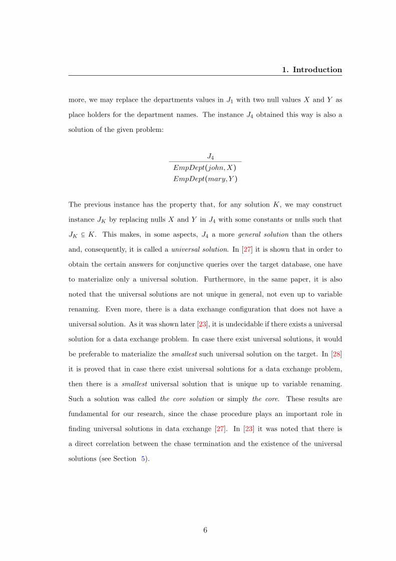
more, we may replace the departments values in J1 with two null values X and Y as
place holders for the department names. The instance J4 obtained this way is also a
solution of the given problem:
J4
EmpDept(john,X)EmpDept(mary,Y )
The previous instance has the property that, for any solution K, we may construct
instance JK by replacing nulls X and Y in J4 with some constants or nulls such that
JK ⊆ K. This makes, in some aspects, J4 a more general solution than the others
and, consequently, it is called a universal solution. In [27] it is shown that in order to
obtain the certain answers for conjunctive queries over the target database, one have
to materialize only a universal solution. Furthermore, in the same paper, it is also
noted that the universal solutions are not unique in general, not even up to variable
renaming. Even more, there is a data exchange configuration that does not have a
universal solution. As it was shown later [23], it is undecidable if there exists a universal
solution for a data exchange problem. In case there exist universal solutions, it would
be preferable to materialize the smallest such universal solution on the target. In [28]
it is proved that in case there exist universal solutions for a data exchange problem,
then there is a smallest universal solution that is unique up to variable renaming.
Such a solution was called the core solution or simply the core. These results are
fundamental for our research, since the chase procedure plays an important role in
finding universal solutions in data exchange [27]. In [23] it was noted that there is
a direct correlation between the chase termination and the existence of the universal
solutions (see Section 5).
6

1. Introduction
1.1.2 Data Repair
Data repair is the transformation process applied to an inconsistent database instance
such that the resulting instance is consistent and it differs ”minimally” from the initial
instance. In this case, the consistency of a database instance is considered against a
set of integrity constraints over the database schema. Such constraints may be: key,
foreign-key, join, or more generally, any constraints specified by a set of embedded
dependencies. Let us denote by Σ the set of constraints. Based on the ”minimality”
restrictions used when comparing the repair with the initial instance, we differentiate
the following types of repairs:
• Superset repair. An instance J is said to be a superset repair of an instance I with
respect of Σ, if instance J contains all tuples from I, satisfies all constraints in Σ,
and there is no other instance J ′ properly contained in J with these properties.
• Subset repair. An instance J is said to be a subset repair of an instance I with
respect of Σ, if instance J contains only tuples from I, satisfies all constraints in
Σ, and there is no other instance J ′ properly containing J with these properties.
• Symmetric-difference repair. An instance J is said to be a symmetric-difference
repair of an instance I with respect to Σ, if instance J is obtained by adding and
removing tuples to/from I, satisfies all constraints in Σ, and there is no other
instance J ′ obtained from a subset of steps used to obtain instance J .
Figure 1.2 gives a visual representation of the aforementioned repair problems, where
Σ represents the set of constraints, S represents the database schema, I the initial
instance and instance J represents a superset, subset and symmetric-difference repairs
respectively.
A general point of view of the literature introducing the types of repairs is, of course,
necessary. The research makes it obvious that data repair represents a major interest
7

1. Introduction
Figure 1.2: Data Repair
in this area. The symmetric-difference repair was introduced by Arenas et al. in [8].
The subset repair as studied by Chomicki and Marcinkowski in [21] requires the repair
to be a maximal consistent subset of the inconsistent instance. In [37] the superset
repair problem is tackled. Lopatenko and Bertossi, in [57], also consider cardinality
repairs, where the repair is to be a subset of maximal cardinality. Afrati and Kolaitis,
in [4], recently introduced the component-cardinality repair which is similar to the
cardinality repair except that it considers the cardinality of each relation separately.
The data complexity of checking if a given instance is a cardinality repair for a given
set of constraints is coNP-hard even for simple sets of constraints. For this reason
we will not cover this type of repairs in our thesis. As we will see in section 5.2, the
chase process plays an important role in determining the existence and checking if an
instance is a subset/superset/symmetric-difference repairs for a given instance under a
set of constraints.
To exemplify the difference between the three data repairs mentioned before let us
consider the following trivial example. The database schema S consisting of two relation
names {Emp,EmpDept}, similarly to the data exchange example, considers also in-
stance the I with tuples I = {Emp(ben),Emp(john),Emp(mary),EmpDept(ben, hr)}.
Consider the constraints on schema S specified by the following formula:
8
1. Introduction
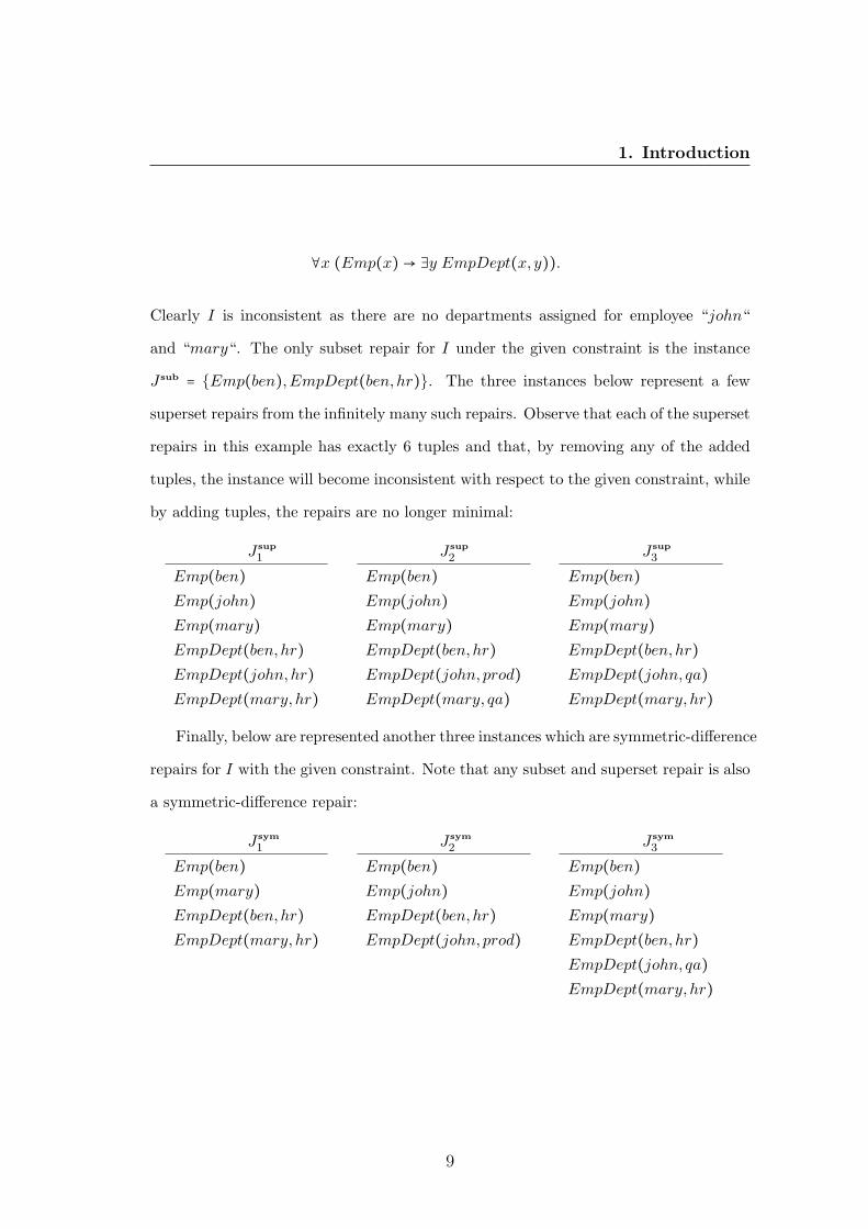
∀x (Emp(x) → ∃y EmpDept(x, y)).
Clearly I is inconsistent as there are no departments assigned for employee “john“
and “mary“. The only subset repair for I under the given constraint is the instance
J sub = {Emp(ben),EmpDept(ben, hr)}. The three instances below represent a few
superset repairs from the infinitely many such repairs. Observe that each of the superset
repairs in this example has exactly 6 tuples and that, by removing any of the added
tuples, the instance will become inconsistent with respect to the given constraint, while
by adding tuples, the repairs are no longer minimal:
J sup
1
Emp(ben)Emp(john)Emp(mary)EmpDept(ben, hr)EmpDept(john,hr)EmpDept(mary, hr)
J sup
2
Emp(ben)Emp(john)Emp(mary)EmpDept(ben, hr)EmpDept(john, prod)EmpDept(mary, qa)
J sup
3
Emp(ben)Emp(john)Emp(mary)EmpDept(ben, hr)EmpDept(john, qa)EmpDept(mary, hr)
Finally, below are represented another three instances which are symmetric-difference
repairs for I with the given constraint. Note that any subset and superset repair is also
a symmetric-difference repair:
J sym
1
Emp(ben)Emp(mary)EmpDept(ben, hr)EmpDept(mary, hr)
J sym
2
Emp(ben)Emp(john)EmpDept(ben, hr)EmpDept(john, prod)
J sym
3
Emp(ben)Emp(john)Emp(mary)EmpDept(ben, hr)EmpDept(john, qa)EmpDept(mary, hr)
9

1. Introduction
1.2 Thesis Structure
Our thesis is structured in two main parts. The first one, covered by chapters 3 and 4,
presents the chase algorithm. Based on its applicability and performance in different
cases, the chase algorithm comes in different variations. Chapter 3 is dedicated to the
reviewing of the most used of these chase variations and to the highlighting of their
difference. It is well known that the chase algorithm does not always terminate. Even
more, it is also known that testing if the chase algorithm terminates is undecidable
in general [23]. In Chapter 4 we revisit the most recent work related to the chase
termination and present the main known classes of dependencies for which the standard-
chase algorithm termination is guaranteed on all instances. In the same chapter we
also investigate if these classes of dependencies ensure termination for different chase
variations already introduced in Chapter 3.
The second part of the thesis is reserved to the some of the applications of the
chase procedure. More precisely, chapter 5 shows why the chase algorithm plays an
important role in data exchange, data repair and the newly introduced data correspon-
dence problems. This is followed by Chapter 6 where we introduce a chase variation
that relies on a new closed world semantics, the constructible models semantics. This
new chase variation helps, in data exchange, to materialize a conditional table over
the target schema used to get the certain answer for general first order queries (FO)
over the target instance compared to the standard chase that materializes an instance
over the target schema used only to get the certain answer for union of conjunctive
queries (UCQ). In Chapter 7 we extend the standard-chase algorithm for second-order
tuple-generating-dependencies under a closed world semantics and show that st-SO de-
pendencies with a target richly acyclic set of TGD’s represent a strong data exchange
system. Finally, Chapter 8 is allocated for conclusions and further work related to the
chase procedure and its applications.
10
1. Introduction
1.3 Contributions
This dissertation covers the results published by the author in [37; 38; 39; 40; 67] ( first
four being a joint work with prof. Gosta Grahne). In this thesis we review the most
prominently used chase variations and make a clear distinction between them based on
the followings:
(a) the result computed by the chase and
(b) the chase algorithm termination.
Part of this study was first presented in [67]. It is well known that the problem of
deciding if the standard-chase procedure terminates1 for a given instance is undecidable
[23]. In Chapter 4 we show that this undecidability result can be extended to the
oblivious-chase algorithm. The chase termination undecidability result motivated the
research community to find classes of dependencies that ensure the chase termination
[23; 27; 59; 61; 63; 70]. Most of these classes guarantee the chase termination for the
standard chase or parallelized standard chase. Unfortunately, none of these classes of
dependencies ensure the termination for the oblivious-chase algorithm. In this thesis
we extend this set of classes of dependencies by unveiling a class of dependencies that
ensures the oblivious-chase termination for all input instances. As it will be shown in
Chapter 6, this class of dependencies lays the foundation of the more restrictive class
of dependencies ensuring that the newly introduced conditional-chase terminates.
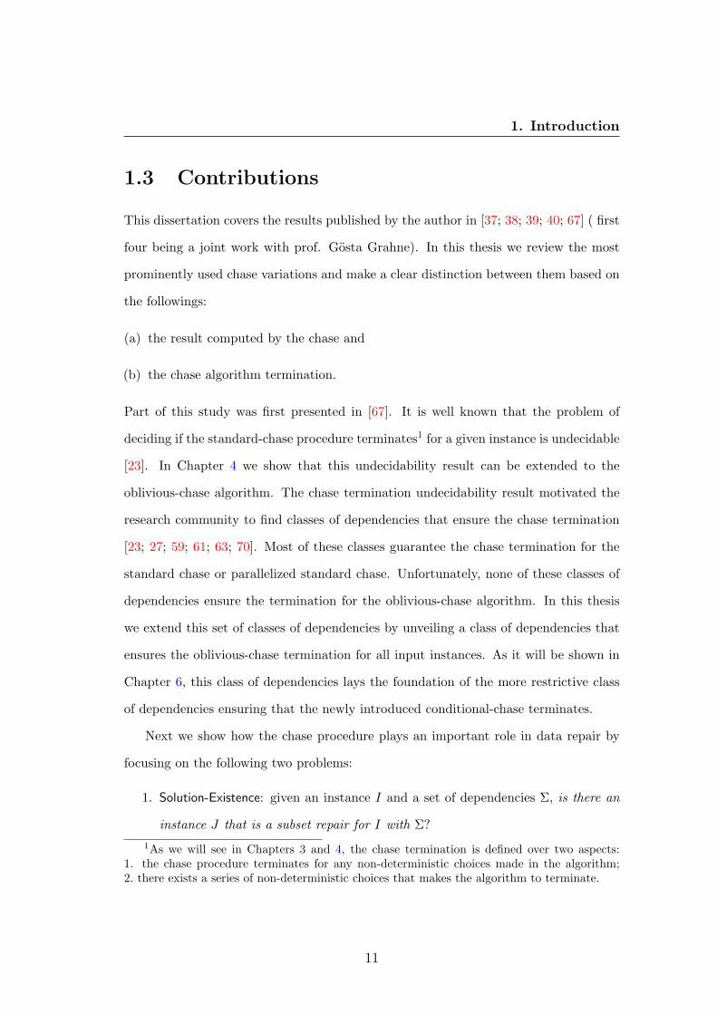
Next we show how the chase procedure plays an important role in data repair by
focusing on the following two problems:
1. Solution-Existence: given an instance I and a set of dependencies Σ, is there an
instance J that is a subset repair for I with Σ?1As we will see in Chapters 3 and 4, the chase termination is defined over two aspects:
1. the chase procedure terminates for any non-deterministic choices made in the algorithm;2. there exists a series of non-deterministic choices that makes the algorithm to terminate.
11

1. Introduction
2. Solution-Check: given the instances I,J and a the set of dependencies Σ, is J a
superset/subset/symmetric-difference repair for I with Σ?
We evaluate these problems when Σ is specified by a set of weakly acyclic tuple
generating dependencies, a class of dependencies that ensures the standard-chase algo-
rithm termination for any input instance. For this class of dependencies, we show that
the subset repair existence problem can be solved in polynomial time. On the other
hand, testing if an instance is a subset or symmetric-difference solution was proved [4]
to be an NP-complete problem (data complexity) for the same class of dependencies.
More recently, this work was also extended by computing consistent answers over the
data repairs [72]. In this thesis we extend the data complexity results by showing that
the NP-completeness result also holds for the superset repair. Next, we introduce a
new large class of dependencies, called semi-LAV, that properly contains both full and
weakly acyclic LAV1 dependencies. For this new class of dependencies we show that
there exists a polynomial time algorithm able to decide all the previously presented
problems.
In Chapter 5 we introduce and investigate a new problem with large practical
implications, the data correspondence problem. Part of this work was first presented
in [37]. Data correspondence is a generalization of data exchange [27] and peer data
exchange [11], and a special case of the data repair problem. More specifically, data
correspondence is the constructive testing between two (or more) database instances in
order to verify if they represent the same information. The challenge arises when the two
databases may be structured according to different schemata. The prototypical example
is to compare a decomposed, normalized instance to the initial universal instance.
As an example, consider the following concrete scenario from a virtual financial
brokerage firm where the employees enter their working hours into a database with the
1We allow duplicated variables in the body for LAV dependencies.
12

1. Introduction
following schema:
EmpHours(EmpId,ProjId,TotHours)HourlyRate(EmpId,Rate)Sponsor(MgrId, ProjId)ExpenseP lan(PlanId, Rate)
The relation EmpHours specifies that an employee with EmpId worked on the project
ProjId for a total of TotHours. Then, the relation HourlyRate records the hourly
salary of the employee on a project. We have a tuple associated with each project in
the relation Sponsor, with the meaning that the project ProjId is sponsored from the
funds of the manager with MgrId. The relation ExpenseP lan represents, of course,
the hourly rate used for different expense plans. On the other hand, the Managers have
to justify their use of funds by entering data in a different database with the schema:
Contribution(MgrId,EmpId,TotHours,Rate)
meaning that the manager with MgrId has paid the employee with EmpId for TotHours
hours at the rate of Rate. In order to verify that funds have been appropriately dis-
persed, the company relies on the constraints specified by the following logical expres-
sions:
∀ei ∀pi ∀th ∀mi ∀r (EmpHours(ei, pi, th) ∧ Sponsor(mi, pi) ∧HourlyRate(ei, r)
�→ Contribution(mi, ei, th, r)),
∀mi ∀ei ∀th ∀r (Contribution(mi, ei, th, r)
�→ ∃pl HourlyRate(ei, r) ∧ExpenseP lan(pl, r)).
If the two instances do not satisfy the given set of dependencies, the company
needs to bring the two database instances up to date, by entering some missing tuples
in the employee database (assuming that the managers financial reports are correct).
13
1. Introduction
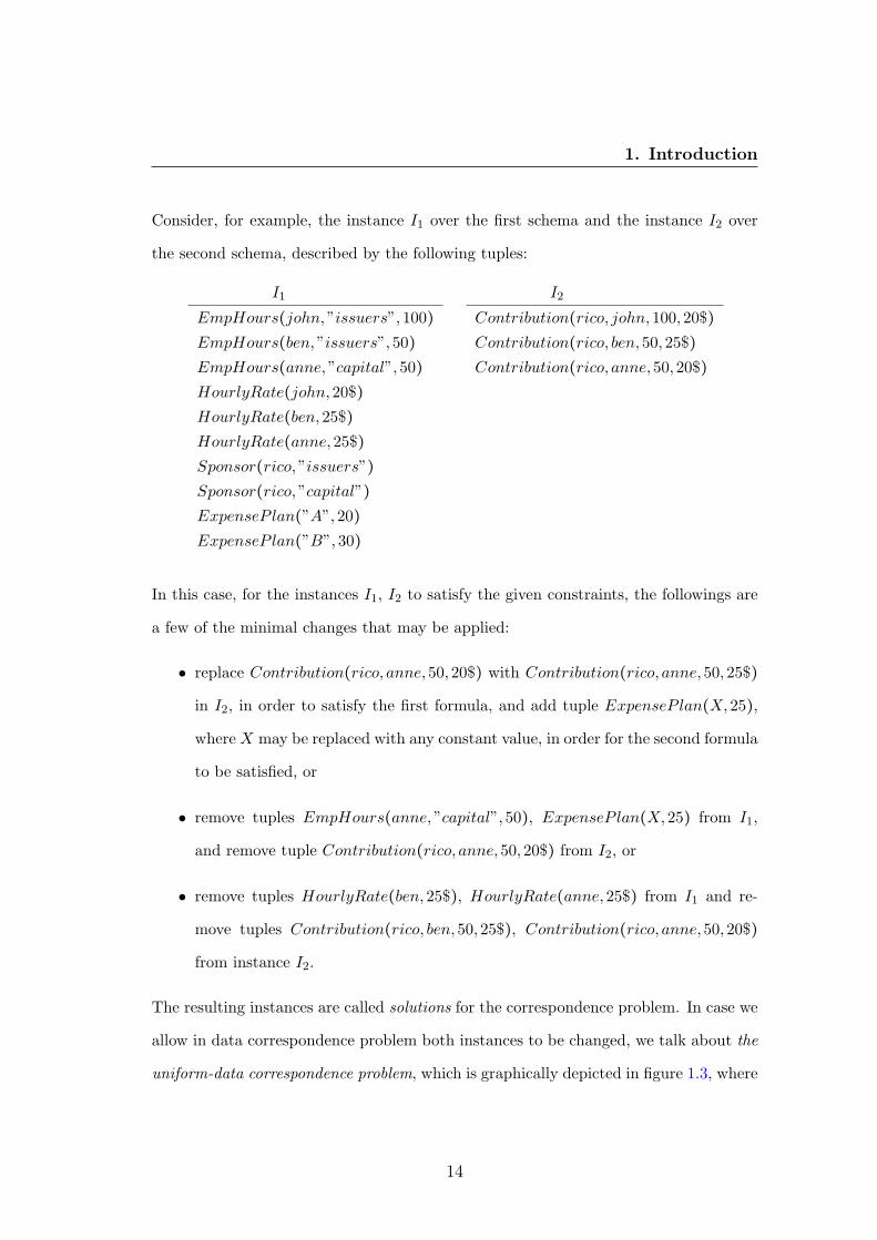
Consider, for example, the instance I1 over the first schema and the instance I2 over
the second schema, described by the following tuples:
I1
EmpHours(john,”issuers”,100)EmpHours(ben,”issuers”,50)EmpHours(anne,”capital”,50)HourlyRate(john,20$)HourlyRate(ben,25$)HourlyRate(anne,25$)Sponsor(rico,”issuers”)Sponsor(rico,”capital”)ExpenseP lan(”A”,20)ExpenseP lan(”B”,30)
I2
Contribution(rico, john,100,20$)Contribution(rico, ben,50,25$)Contribution(rico, anne,50,20$)
In this case, for the instances I1, I2 to satisfy the given constraints, the followings are
a few of the minimal changes that may be applied:
• replace Contribution(rico, anne,50,20$) with Contribution(rico, anne,50,25$)
in I2, in order to satisfy the first formula, and add tuple ExpenseP lan(X,25),
where X may be replaced with any constant value, in order for the second formula
to be satisfied, or
• remove tuples EmpHours(anne,”capital”,50), ExpenseP lan(X,25) from I1,
and remove tuple Contribution(rico, anne,50,20$) from I2, or
• remove tuples HourlyRate(ben,25$), HourlyRate(anne,25$) from I1 and re-
move tuples Contribution(rico, ben,50,25$), Contribution(rico, anne,50,20$)
from instance I2.
The resulting instances are called solutions for the correspondence problem. In case we
allow in data correspondence problem both instances to be changed, we talk about the
uniform-data correspondence problem, which is graphically depicted in figure 1.3, where
14

1. Introduction
S1 and S2 represent the two database schemata; Σ12 and Σ21 the set of constraints; I1
and I2 the initial instances; and I ′1, I ′2 represent some superset solutions for the uniform-
data correspondence problem. Note that the uniform-data correspondence problem can
be viewed as a special case of data repair problem [4; 8; 21].
Figure 1.3: Uniform-Data Correspondence
In some cases, one of the sources needs to be authoritative, meaning that it is
sound and complete and can not therefore be modified. By considering in the previous
example, for the second source to be authoritative, we can apply the following mini-
mal transformation to I1 (the non-authoritative instance) in order to satisfy the given
constraints: remove tuple HourlyRate(anne,25$), add tuples HourlyRate(anne,20$)
and ExpenseP lan(X,25). This correspondence problem is called the non-uniform-data
correspondence problem and it is graphically depicted in figure 1.4. Even if the non-
uniform-data correspondence problem looks similar to the peer data exchange problem
[11] they are different in the sense that for the non-uniform correspondence problem
we are looking for ”minimal” solution rather than superset solutions. In the follow-
ing, by mentioning data correspondence problem we refer to both uniform-data and
non-uniform-data cases.
Similarly to the data repair problem, for the data correspondence problem we con-
sider the superset, subset and symmetric-difference solutions cases. From the previous
15

1. Introduction
Figure 1.4: Non-Uniform-Data Correspondence
example we observe that there may be several solutions to the correspondence prob-
lem; however it may also be the case that there does not exist any solution. We will
show in Section 5.3 that the chase procedure plays an important role in checking the
existence of solutions and also in testing if a pair of instances is a solution for a data
correspondence problem.
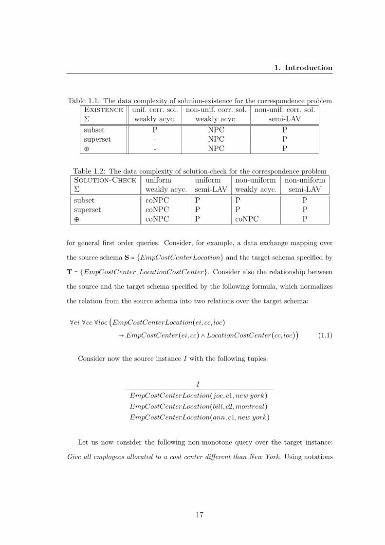
Similarly to data repair, we investigate the problem of deciding if there exists a solu-
tion and the problem of testing if a given pair of ground instances is a solution for both
uniform and non-uniform data correspondence settings. Tables 1.1 and 1.2 summarize
the data complexity results found for these problems under weakly acyclic and semi-
LAV classes of dependencies. The coNP-completeness data complexity result occurs
for the symmetric-difference solution-check for the non-uniform-data correspondence
problem under a weakly acyclic set of dependencies. This result is rather surprising
considering that the subset and superset solution-check problems are both polynomial
under same settings. Also, from the complexity results table, it can be noted that the
new class of semi-LAV dependencies is tractable for all previously mentioned problems.
The data exchange problem, as first presented in [27], relies on an open world
semantics. Following that, one may get only certain answers for union of conjunctive
queries. As we can see in the following example, the open world semantics is not suitable
16
1. Introduction
Table 1.1: The data complexity of solution-existence for the correspondence problemExistence unif. corr. sol. non-unif. corr. sol. non-unif. corr. sol.Σ weakly acyc. weakly acyc. semi-LAV
subset P NPC Psuperset - NPC P⊕ - NPC P
Table 1.2: The data complexity of solution-check for the correspondence problemSolution-Check uniform uniform non-uniform non-uniformΣ weakly acyc. semi-LAV weakly acyc. semi-LAV
subset coNPC P P Psuperset coNPC P P P⊕ coNPC P coNPC P
for general first order queries. Consider, for example, a data exchange mapping over
the source schema S = {EmpCostCenterLocation} and the target schema specified by
T = {EmpCostCenter,LocationCostCenter}. Consider also the relationship between
the source and the target schema specified by the following formula, which normalizes
the relation from the source schema into two relations over the target schema:
∀ei ∀cc ∀loc (EmpCostCenterLocation(ei, cc, loc)
→ EmpCostCenter(ei, cc) ∧LocationCostCenter(cc, loc)) (1.1)
Consider now the source instance I with the following tuples:
I
EmpCostCenterLocation(joe, c1, new york)EmpCostCenterLocation(bill, c2,montreal)EmpCostCenterLocation(ann, c1, new york)
Let us now consider the following non-monotone query over the target instance:
Give all employees allocated to a cost center different than New York. Using notations
17

1. Introduction
from [1], this query can be expressed as:
ans(ei) ← EmpCostCenter(ei, cc),¬LocationCostCenter(cc,“New Y ork“) (1.2)
The certain answer to this query will be empty under the OWA semantics . On the
other hand, as each employee may belong to a single cost center and each cost center
is uniquely located, we may expect that query 1.2 returns as certain answer “bill“.
Realizing that the open world semantics had some anomalies, Libkin [54] proposed a
first CWA semantics for data exchange; his work was followed by [44; 45; 47; 56]. In
this thesis we continue this line of work by proposing a new CWA semantics, called
constructible solution semantics, which we argue is a natural fit for the data exchange
problem. Intuitively constructible solution semantics only considers those tuples in the
target instance that can be constructed from the source instance. We will show that the
instance based representation is not enough to capture the new CWA semantics and
we extend this by using conditional tables as representation of the possible solutions.
Where the conditional tables are structures that extend tabular instances by associating
local conditions for each tuple, such that a tuple exists under some valuation if the
local condition is evaluated to true. Next, we extend the chase procedure to properly
capture this new semantics. To illustrate this, consider the relationship between source
and target schema specified by the following source-to-target dependency:
∀ei (Employee(ei) → ∃mi EmpMgr(ei,mi)) (1.3)
and the target dependency:
∀ei (EmpMgr(ei, ei) → SelfMgr(ei)) (1.4)
18

1. Introduction
The following two instances correspond to the target representation of the source
instance I = {employee(john), employee(ann)} when chasing I with the standard chase
and with new conditional chase respectively:
J
EmpMgr(john,X)EmpMgr(ann,Y )
t ϕ(t)
EmpMgr(john,X) true
EmpMgr(ann,Y ) true
SelfMgr(john) X = john
SelfMgr(ann) Y = ann
As it can be seen, the standard-chase algorithm with the input dependencies 1.3 and
1.4 can not capture the possibility that the employees ”john” and ”ann” can be their
own manager. We introduce a new class of dependencies that ensures the conditional-
chase termination for any input instances and then relates the conditional-chase termi-
nation to the oblivious-chase termination.
Finally, in the last chapter we focus on the representation systems for data exchange.
The notion of representation systems describes structures that are algebraically closed
under queries. We extend the notion of representation system to encompass data ex-
change mappings. Seen through this lens, two major classes of representation systems
emerge, namely homomorphic data exchange systems and strong data exchange sys-
tems. The monotone systems encompass the classical OWA data exchange semantics,
in which reasoning is modulo homomorphic equivalence and only union of conjunctive
queries are supported. We develop new technical tools that allow us to prove that
there is a class of CWA strong representation systems in which reasoning is modulo
isomorphic equivalence. These systems are based on conditional tables and support
first-order queries and data exchange mappings specified by a large class of second-
order dependencies. We achieve this by showing that under the constructible models
closed world semantics, conditional tables are chaseable with the aforementioned class
of second-order dependencies.
19

Chapter 2
Notations and Preliminaries
This chapter covers the notations and notions used in our thesis. Let N denote the
set of natural numbers. We use as placeholders for natural numbers lowercase letters,
possibly subscripted and/or superscripted (for example i,kn,mlj). For any two natural
numbers n,m with m ≤ n let [m,n] be the set of all natural numbers p with m ≤ p ≤ n.
The set [1, n] is also denoted by [n]. For a set A, by ∣A∣ we denote its cardinality, and
by P(A) we identify its powerset, that is all subsets of A. By “⊕“ we represent the
symmetric difference operator between sets. Thus for two sets A and B by A ⊕B we
mean the set (A∖B) ∪ (B ∖A). For a given set I, we say that A ≤I B if A⊕ I ⊆ B ⊕ I.
Clearly ≤I , for a given set I, is a partial order over sets. We say that sets A and B
are incomparable, denoted A ∦ B, if A ⊈ B and B ⊈ A. A tuple a over a set A is a
sequence of the form (a1, . . . , an), with ai ∈ A for all i ∈ [n]. The length of a tuple a,
denoted ∣a∣, is the number of elements in a. By abusing the notation, we sometimes
treat tuples as sets, that is we write a ∈ a to denote that element a is part of the
tuple, and we write a ⊆ A to denote that all elements in a are in set A. Given two
sets A, B and the mapping f ∶ A → B, we define Dom(f) = A (the domain of f) and
Im(f) = {f(a) ∣ a ∈ Dom(f)} (the image of f), clearly Im(f) ⊆ B. We sometimes
20

2. Notations and Preliminaries
specify a mapping f as {a1/f(a1), . . . , an/f(an)}, where {a1, . . . , an} ⊆ Dom(f) and
for all a ∈ Dom(f) ∖ {a1, . . . , an} we have f(a) = a. A mapping f is said to extend
mapping g, denoted g ⋐ f , if Dom(g) ⊆ Dom(f) and f(a) = g(a) for all a ∈ Dom(g).
For two mappings f and g such that Dom(f) ∩Dom(g) = ∅, by f ⊔ g, we denote the
smallest mapping on the domain Dom(f) ∪Dom(g) such that f ⋐ f ⊔ g and g ⋐ f ⊔ g.
For a set D by Id(D) we denote the identity mapping on D, that is Id(D)(a) = a for
all a ∈ D. By Id we denote the set of all identity mappings. Mappings are extended
to tuples as follows: let f be a mapping and a = (a1, . . . , an) ⊆ Dom(f). By f(a) we
denote the tuple (f(a1), . . . , f(an)). In the natural way, we extend a mapping f to a
set A as follow, f(A) = {f(a) ∣ a ∈ A}, where f(a) is defined for all a ∈ A (note that A
may be a set of tuples, not only elements from Dom(f)).
2.1 Relational Databases
A database schema R, or simply schema, is a finite set {R1, . . . ,Rn} of relation symbols.
For each relation symbol R ∈R, we assign a positive integer arity(R) representing the
relation arity. Let ΔC and ΔN be two disjoint countable infinite sets of constants and
nulls respectively. In this thesis, we will denote the constants by lowercase letters,
possibly subscripted/superscripted, from the beginning of the alphabet (eg. a, b1, . . .).
The nulls are denoted by possibly subscripted/superscripted uppercase letters from the
end of the alphabet (eg. X, Y1, . . .). Let D = ΔC ∪ΔN. A finite instance for a schema
R is a mapping I that assigns for each relational symbol R a finite set of tuples from
Darity(R) (i.e. I(R) ⊆ Darity(R)). In some cases we will also allow instances to assign
infinite sets of tuples, in this case we talk about infinite instances. In this dissertation,
if not mentioned otherwise, by instance we mean a finite instance. If a tuple a belongs
to I(R), we say that R(a) is a fact for I. For ease of notation we will also denote by I
the set of facts for mapping I. We use two distinct tabular representations to specify
21
2. Notations and Preliminaries
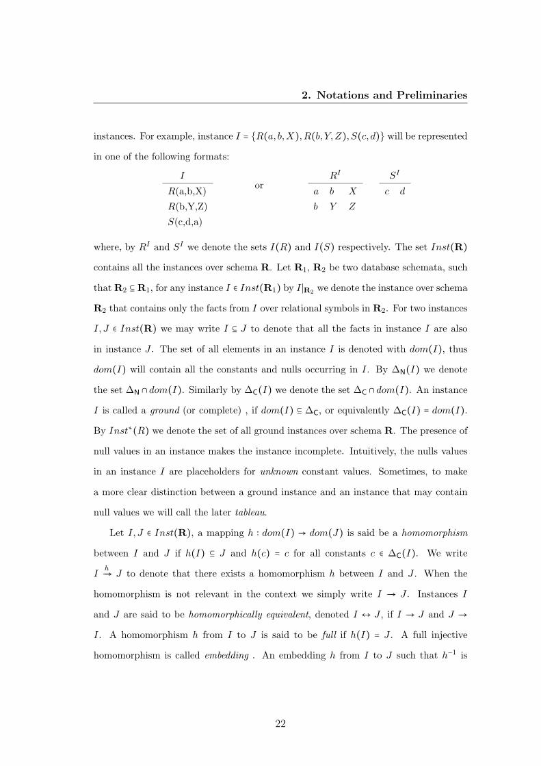
instances. For example, instance I = {R(a, b,X),R(b, Y,Z), S(c, d)} will be represented
in one of the following formats:
I
R(a,b,X)
R(b,Y,Z)
S(c,d,a)
orRI
a b X
b Y Z
SI
c d
where, by RI and SI we denote the sets I(R) and I(S) respectively. The set Inst(R)
contains all the instances over schema R. Let R1, R2 be two database schemata, such
that R2 ⊆R1, for any instance I ∈ Inst(R1) by I ∣R2 we denote the instance over schema
R2 that contains only the facts from I over relational symbols in R2. For two instances
I, J ∈ Inst(R) we may write I ⊆ J to denote that all the facts in instance I are also
in instance J . The set of all elements in an instance I is denoted with dom(I), thus
dom(I) will contain all the constants and nulls occurring in I. By ΔN(I) we denote
the set ΔN ∩ dom(I). Similarly by ΔC(I) we denote the set ΔC ∩ dom(I). An instance
I is called a ground (or complete) , if dom(I) ⊆ ΔC, or equivalently ΔC(I) = dom(I).
By Inst∗(R) we denote the set of all ground instances over schema R. The presence of
null values in an instance makes the instance incomplete. Intuitively, the nulls values
in an instance I are placeholders for unknown constant values. Sometimes, to make
a more clear distinction between a ground instance and an instance that may contain
null values we will call the later tableau.
Let I, J ∈ Inst(R), a mapping h ∶ dom(I) → dom(J) is said be a homomorphism
between I and J if h(I) ⊆ J and h(c) = c for all constants c ∈ ΔC(I). We write
Ih�→ J to denote that there exists a homomorphism h between I and J . When the
homomorphism is not relevant in the context we simply write I �→ J . Instances I
and J are said to be homomorphically equivalent, denoted I ↔ J , if I �→ J and J �→
I. A homomorphism h from I to J is said to be full if h(I) = J . A full injective
homomorphism is called embedding . An embedding h from I to J such that h−1 is
22

2. Notations and Preliminaries
also an embedding from J to I is called isomorphism. Two instances I and J are said
to be isomorphically equivalent if there exists an isomorphism between I and J . This
is denoted by I ≅ J . Note that not all embeddings are isomorphisms. For example,
consider the two instances I = {R(a,X),R(b, Y )} and J = {R(a,Z),R(b, c)}. Clearly
the embedding e = {X/Z,Y /c} is not an isomorphism as e−1(c) = Z, that is e−1 is not
an embedding. A homomorphism h is said to be an extension of homomorphism h if
h ⋐ h.
A homomorphism h from I to I is said to be an endomorphism . A retraction is
a endomorphism h from I to J = h(I) such that h is identity on dom(J), in this case
J is called a retract of I. An instance J is said to be a proper retract of an instance I
if J is a retract of I and J ⊊ I. An instance I is said to be a core if it does not have
any proper retract. An instance J is said to be a core of I, if J is a retract of I and
it is also a core. The cores of an instance I are unique up to isomorphism [27; 43] and
therefore we can talk about the core of an instance I and denote it core(I).
2.2 Queries
Consider ΔV to be a countable infinite set of variables, such that it is disjoint of ΔC and
ΔN. In this dissertation we will denote the variables with lowercase letters, possibly
subscripted/superscripted, from the end of the alphabet (eg. x, z1, y2, . . .). A relational
atom , or simply atom, over schema R is an expression of the form R(x), where R ∈R
and x is a tuple from (ΔC⋃ΔV)arity(R). A conjunctive query q over schema R is an
expression of the form:
q(x) ← R1(x1), . . . ,Rn(xn) (2.1)
where for all i ∈ [n] we have Ri(xi) which is an atom over R; the elements in x are from
23

2. Notations and Preliminaries
the set ΔC⋃ΔV, and all variables in x appear in at least one tuple xi, i ∈ [n]. The size
∣x∣ represents the arity of the query q, denoted with arity(q). By CQ we denote the set
of all conjunctive queries over any schema. The semantics for a conjunctive query q on
a ground instance I ∈ Inst∗(R) is defined as, where a valuation is a mapping identity
on constants and its image is over constants:
q(I) = {v(x) ∣ v - valuation, and v(xi) ∈ I(Ri), ∀i ∈ [n]} (2.2)
In case ∣x∣ = 0, then we say that q is a boolean query . The semantics for a boolean
query q on a ground instance I is:
q(I) =⎧⎪⎪⎨⎪⎪⎩
true if ∃v - valuation, and v(xi) ∈ I(Ri), ∀i ∈ [n]false otherwise
(2.3)
For a conjunctive query q ∈ CQ, we denote by db(q) the instance containing the
facts Ri(Xi), i ∈ [n], where Xi is obtained from xi by replacing each variable with a
fresh new null from ΔN. Consider the following query:
q(x1, x3, x5) ← R(a, x1, x2), S(x2, x3),R(x3, x4, x5), T (x5, b) (2.4)
For this query we have db(q) = {R(a,X1,X2), S(X2,X3),R(X3,X4,X5), T (X5, b)}. Re-
call that the variables are denoted with lowercase letters and the nulls with uppercase
letters.
Consider q1,. . ., qn be n conjunctive queries with the same arity. Then a query
Q specified as Q ← q1 ∨ . . . ∨ qn is called a union of conjunctive queries and has the
following semantics: Q(I) = q1(I) ∪ . . . ∪ qn(I). By UCQ we denote the set of all union
of conjunctive queries. For a better distinction, in this thesis, we will denote conjunc-
tive queries with lowercase letters and union of conjunctive queries with upper case
letters. For a query Q ∈ UCQ, Q ← q1 ∨ . . .∨ qn, we define db(Q) = {db(q1), . . . , db(qn)}.
24
2. Notations and Preliminaries
By CQ≠ is denoted the set of all conjunctive queries that also allow the unequality
atom. The extension of the previous classes of queries by allowing negated atoms gives
CQ¬,UCQ¬,CQ¬,≠ and UCQ¬,≠. The semantics of these types of queries is naturally ex-
tended from the semantics of conjunctive queries. A more detailed description of these
semantics can be found in [1].
Note that the query semantics previously defined mentions only ground instances,
that is complete databases. An incomplete database (over a schema R) is conceptually
a set I of ground instances (over schema R), or possible worlds I. Given a query q and
an incomplete database I, the result of q on I is q(I) = {q(I)∣ I ∈ I}. To this exact
answer [36] there are two approximations [48], namely:
• certain answer evaluation: certain(q,I) = ⋂I∈I q(I), and
• possible answer evaluation: possible(q,I) = ⋃I∈I q(I).
In some cases an incomplete database I over schema R can be specified by a single,
not necessarily ground, instance I such that
I = {J ∣ v is a valuation, v(I) ⊆ J, J ∈ Inst∗(R)}
Where a valuation v is mapping with domain ΔC ∪ ΔN and image ΔC. In this case,
for any query q ∈ UCQ, the certain answer certain(q,I) can be computed by executing
these two steps [27]: a) evaluate q on instance I by treating each null values as a new
constant; b) the certain answer result will contain all the tuples from the previous
evaluation that contains only constants. Libkin showed in [55] that UCQ is the largest
class of queries for which the certain answer can be evaluated in this way. In [1; 35] it is
also shown that if I is specified by instance I, J is specified by instance J and I ↔ J ,
then certain(q,I) = certain(q,J ) for any q ∈ UCQ. Thus, if two incomplete instances
are represented by two homomorphically equivalent instances, then the certain answers
for any union of conjunctive query will be the same for both incomplete databases.
25

2. Notations and Preliminaries
Given Q ∈ UCQ over database schema R and instance I ∈ Inst(R) we say that I is
a model for Q, denoted I ⊧ Q, if there exists instance J ∈ db(Q) such that J → I.
2.3 Dependencies
In most real life applications, database schemata have attached a set of constraints that
needs to be satisfied by each instance over the given schema. Some of the most fre-
quent constraints of this type are: primary-key, foreign-key and functional dependency.
It is very common to use first order logic as a representation language for database
constraints.
In this dissertation we will focus mainly on constraints specified as embedded de-
pendencies (for a survey on database dependencies see [31]). An embedded dependency
over schema R is a first order sentence ξ of the form:
∀x,∀y (α(x, y) → ∃z β(x, z)) (2.5)
where all variables in x appear both in α and β. The expression α is a conjunction of
possible negated relational atoms over R and unequalities atoms. The expression β is
a first order expression over relational atoms over R, unequalities and equalities atoms.
We usually refer to the formula given by α as the body of the embedded dependency,
and the formula given by β as the head of the dependency.
The following subclasses of embedded dependencies play an important role in rep-
resenting database constraints:
• A tuple-generating-dependency (TGD) is an embedded dependency where both
the body and the head are formulae logically equivalent with a conjunction of
relational atoms;
• An equality-generating-dependency (EGD) is an embedded dependency where the
26
2. Notations and Preliminaries
body is a formula logically equivalent with a conjunction of relational atoms and
the head is represented by an equality atom;
• A tuple-generating-dependency with disjunctions (TGD∨) is an embedded de-
pendency where the body is a formula logically equivalent with a conjunction
of relational atoms and the head is equivalent with a disjunction of the form
β1 ∨ β2 ∨ . . . βn where, for all i ∈ [n], βi is a conjunction of relational atoms;
• A tuple-generating-dependency with negations (TGD¬) is a tuple generating de-
pendency where we allow negated relation atoms both in the body and the head;
• A tuple-generating-dependency with negations and disjunctions (TGD∨,¬) is a
tuple-generating-dependency with disjunctions where we also allow negated re-
lation atoms in the body and the head.
The following three subclasses of TGD are also of importance in our work:
• A full TGD is a TGD without any existentially quantified variables;
• A local-as-view dependency (LAV) is a TGD with only one relational atom in
the body of the dependency;
• A true-local-as-view dependency (LAV∗) is a LAV dependency without repeating
variables in the body;
Sometimes, when referring to a generic tuple-generating-dependency, we may also
use the notation α → β; and when referring to an equality-generating-dependency, we
use the notation α → x = y. For simplicity we will omit the universal quantifiers; also
the conjunction between atoms will be denoted by comma. For example the embedded
dependency:
∀x∀y∀z (R(x, y, z) ∧ S(y, z) → ∃v (R(v, y, z) ∧ S(v, z)) ∨ (R(x, y, v) ∧ ¬S(v, z)))
27

2. Notations and Preliminaries
will be simply denoted as:
R(x, y, z), S(y, z) → ∃v R(v, y, z), S(v, z) ∨R(x, y, v),¬S(v, z)
Given two distinct schemata R1 and R2, a set Σ of TGD’s is said to be source-
to-target TGD’s if the relational symbols in the body of each dependency are from
schema R1 and the relational symbols in the head of each dependency are from schema
R2. In this case we say that Σ is a set of source-to-target dependencies over schema
(R1,R2).
For a schema R, by TGD(R) we denote the set of all TGD’s over schema R. Sim-
ilarly are defined the dependency class restrictions to a database schema. An instance
I is said to satisfy a set of embedded dependencies Σ, denoted I ⊧ Σ, if I satisfies all
dependencies in Σ in the standard model theoretic sense.
Finally, given a tuple-generating-dependency ξ of the form α(x, y) → ∃z β(x, z), by
body(ξ) we denote the instance containing the tuples obtained by replacing all variables
in the relational atoms from the body of the dependency with fresh new null values.
Similarly, by head(ξ) we denote the instance obtained from the head of the dependency.
In case ξ ∈TGD∨, head(ξ) represents a set of instances corresponding to each disjunct
in the head of the dependency. For ease of reference, we consider that each variable
x from ξ is replaced by null X in body(ξ) and head(ξ) (that is each variable name
from the dependency is kept with the same as null in the instance but upper case, thus
the same variable is mapped to the same null both in the body and the head of the
dependency).
28

Chapter 3
The Chase Procedure
3.1 The Chase Procedure
The chase procedure is an iteration a chase steps that either adds a new tuple to satisfy
a TGD, either changes the instance to model some equality-generating-dependency,
or fails when the instance could not be changed to satisfy an equality-generating-
dependency. Depending on when or how the chase step is applied, different chase
variations have been considered lately [16; 23; 27; 38; 59; 63]. To differentiate be-
tween the variations of the chase procedure, we will call the the standard chase the
chase procedure considered by Fagin et al [27] for the data exchange problem. Most of
the practical constraints in databases can be represented as a set of tuple-generating
(TGD) and equality-generating (EGD) dependencies. The first part of this chapter is
devoted to present the chase procedure applied on an instance over a set of of TGD’s
and EGD’s. Later on, in Section 3.2, we will also consider the chase under other types
of dependencies such as TGD∨, TGD¬ and TGD∨,¬ (as defined in the preliminar-
ies). For ease of notation, through this section, if not mentioned otherwise, we will use
the notation I to represent an arbitrary instance and Σ to represent an arbitrary set of
29

3. The Chase Procedure
TGD’s and EGD’s over the same schema. Also, the database schema will be explicitly
mentioned if it is not obvious from the context. Part of this section was also published
in [67].
3.1.1 The Chase Step
As stipulated at the beginning of this chapter, the chase procedure is a repetitive
application of a chase step. Each chase step “applies“ a dependency (in this case TGD
or EGD) on a subset of the instance.
3.1.1.1 The TGD Chase Step
Let I be an instance over schema R and let ξ be the TGD: α(x, y) → ∃z β(y, z) over
the same schema R. In this case, it is said that the TGD ξ is applicable to instance I
with homomorphism h if the following two conditions hold:
1. h is a homomorphism between instances body(ξ) and I, i.e. body(ξ)h�→ I and
2. there is no extension h of h such that head(ξ)h�→ I.
If TGD ξ is applicable to I with h, we say that the pair (ξ, h) is a standard TGD
trigger for instance I. In addition, if (ξ, h) is a trigger for I, construct an extension h
of h, such that h(Z) = Z ′, for all nulls Z ∈ Z (recall that each variable x corresponds
to null X in body(ξ) and head(ξ)), with Z ′ a fresh new labeled null from ΔN. The
instance J obtained as J = I ∪ h(head(ξ)) is called the result of applying a standard
TGD chase step on I with trigger (ξ, h). The notation I(ξ,h)���→ J represents a standard
TGD chase step applied on I with trigger (ξ, h).
Example 1 Consider instance I = {R(a, b),R(b, a), S(b, c)} over schema R = {R,S},
and consider TGD ξ: R(x, y),R(y, x) → ∃z S(x, z). For this dependency we have
body(ξ) = {R(X,Y ),R(Y,X)} and head(ξ) = {S(X,Z)}. For these settings there exists
30

3. The Chase Procedure
homomorphism h = {X/a, Y /b} that maps body(ξ) to I; and there is no extension
of h that maps head(ξ) to I. This makes ξ applicable to I with homomorphism h,
yielding the chase step I(ξ,h)���→ J , where J = I ∪{S(a,Z′)} and where the extension h of
homomorphism h maps Z to Z′. Note that the homomorphism h1 = {X/b, Y /a} together
with dependency ξ does not form a trigger for I because there exists h1 extension of h1,
namely h1 = {X/b, Y /a,Z/c}, such that h1(head(ξ)) ⊆ I.
3.1.1.2 The EGD Chase Step
Let I be an instance for schema R, and ξ be the EGD: α(x) → xi = xj , where xi, xj ∈ x.
The EGD ξ is said to be applicable to I with homomorphism h, if the following two
conditions hold:
1. body(ξ)h�→ I and
2. h(xi) ≠ h(xj).
Similarly to the TGD case, the pair (ξ, h) is called an EGD trigger for I, or simply a
trigger for I. For a trigger (ξ, h) over instance I, if h maps both nulls Xi and Xj to
constants, then we say that the EGD chase step fails, and this is denoted as I(ξ,h)���→ %.
In case the homomorphism h does not map both nulls Xi and Xj to (distinct) constants,
then we say that the chase step does not fail. This is denoted with I(ξ,h)���→ J , where
the instance J is computed as follows:
1. If h(Xi) and h(Xj) are both mapped to labeled nulls, then construct instance J
from instance I by replacing either all occurrences of h(Xi) with h(Xj), or all
occurrences of h(Xj) with h(Xi).
31
3. The Chase Procedure
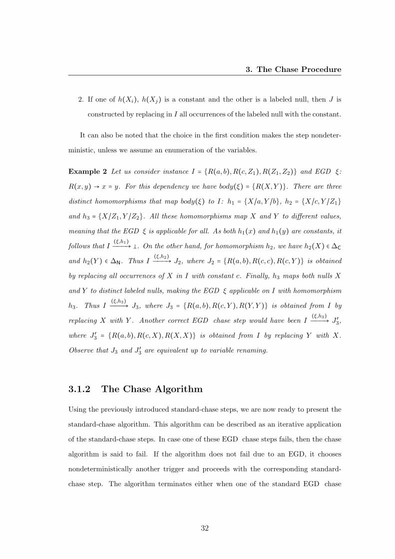
2. If one of h(Xi), h(Xj) is a constant and the other is a labeled null, then J is
constructed by replacing in I all occurrences of the labeled null with the constant.
It can also be noted that the choice in the first condition makes the step nondeter-
ministic, unless we assume an enumeration of the variables.
Example 2 Let us consider instance I = {R(a, b),R(c,Z1),R(Z1, Z2)} and EGD ξ:
R(x, y) → x = y. For this dependency we have body(ξ) = {R(X,Y )}. There are three
distinct homomorphisms that map body(ξ) to I: h1 = {X/a, Y /b}, h2 = {X/c, Y /Z1}
and h3 = {X/Z1, Y /Z2}. All these homomorphisms map X and Y to different values,
meaning that the EGD ξ is applicable for all. As both h1(x) and h1(y) are constants, it
follows that I(ξ,h1)���→ %. On the other hand, for homomorphism h2, we have h2(X) ∈ ΔC
and h2(Y ) ∈ ΔN. Thus I(ξ,h2)���→ J2, where J2 = {R(a, b),R(c, c),R(c, Y )} is obtained
by replacing all occurrences of X in I with constant c. Finally, h3 maps both nulls X
and Y to distinct labeled nulls, making the EGD ξ applicable on I with homomorphism
h3. Thus I(ξ,h3)���→ J3, where J3 = {R(a, b),R(c, Y ),R(Y,Y )} is obtained from I by
replacing X with Y . Another correct EGD chase step would have been I(ξ,h3)���→ J ′
3,
where J ′3 = {R(a, b),R(c,X),R(X,X)} is obtained from I by replacing Y with X.
Observe that J3 and J ′3 are equivalent up to variable renaming.
3.1.2 The Chase Algorithm
Using the previously introduced standard-chase steps, we are now ready to present the
standard-chase algorithm. This algorithm can be described as an iterative application
of the standard-chase steps. In case one of these EGD chase steps fails, then the chase
algorithm is said to fail. If the algorithm does not fail due to an EGD, it chooses
nondeterministically another trigger and proceeds with the corresponding standard-
chase step. The algorithm terminates either when one of the standard EGD chase
32
3. The Chase Procedure
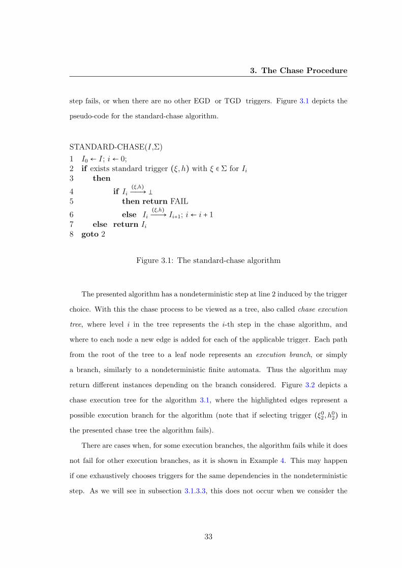
step fails, or when there are no other EGD or TGD triggers. Figure 3.1 depicts the
pseudo-code for the standard-chase algorithm.
STANDARD-CHASE(I,Σ)
1 I0 ← I; i← 0;2 if exists standard trigger (ξ, h) with ξ ∈ Σ for Ii
3 then
4 if Ii
(ξ,h)→ �
5 then return FAIL
6 else Ii
(ξ,h)→ Ii+1; i← i + 1
7 else return Ii
8 goto 2
Figure 3.1: The standard-chase algorithm
The presented algorithm has a nondeterministic step at line 2 induced by the trigger
choice. With this the chase process to be viewed as a tree, also called chase execution
tree, where level i in the tree represents the i-th step in the chase algorithm, and
where to each node a new edge is added for each of the applicable trigger. Each path
from the root of the tree to a leaf node represents an execution branch, or simply
a branch, similarly to a nondeterministic finite automata. Thus the algorithm may
return different instances depending on the branch considered. Figure 3.2 depicts a
chase execution tree for the algorithm 3.1, where the highlighted edges represent a
possible execution branch for the algorithm (note that if selecting trigger (ξ02 , h
02) in
the presented chase tree the algorithm fails).
There are cases when, for some execution branches, the algorithm fails while it does
not fail for other execution branches, as it is shown in Example 4. This may happen
if one exhaustively chooses triggers for the same dependencies in the nondeterministic
step. As we will see in subsection 3.1.3.3, this does not occur when we consider the
33
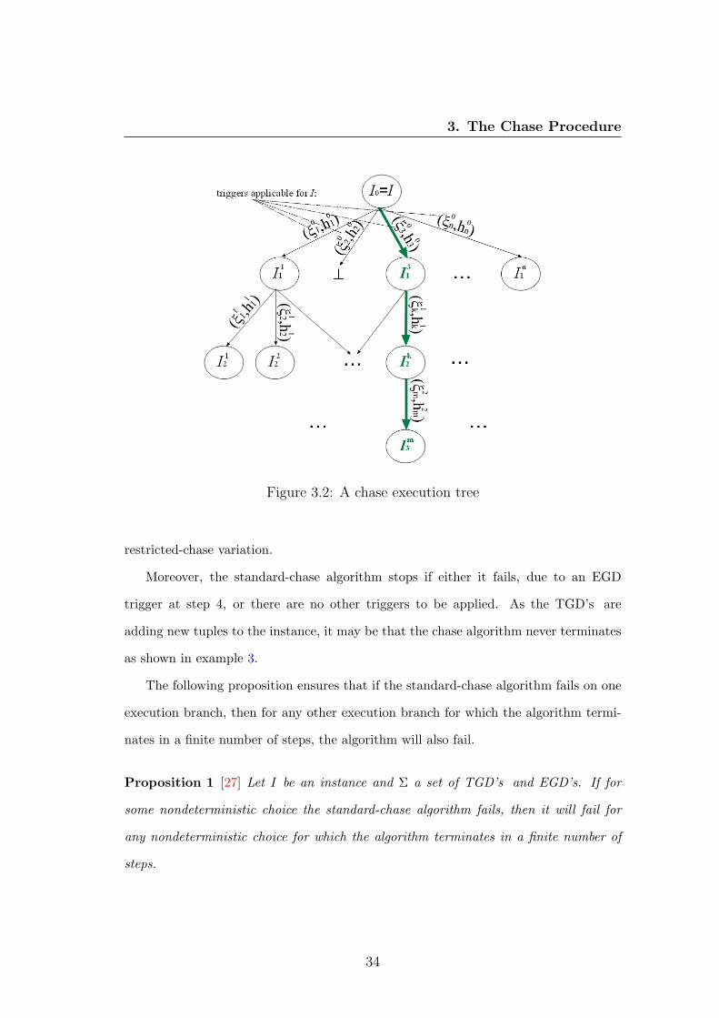
3. The Chase Procedure
Figure 3.2: A chase execution tree
restricted-chase variation.
Moreover, the standard-chase algorithm stops if either it fails, due to an EGD
trigger at step 4, or there are no other triggers to be applied. As the TGD’s are
adding new tuples to the instance, it may be that the chase algorithm never terminates
as shown in example 3.
The following proposition ensures that if the standard-chase algorithm fails on one
execution branch, then for any other execution branch for which the algorithm termi-
nates in a finite number of steps, the algorithm will also fail.
Proposition 1 [27] Let I be an instance and Σ a set of TGD’s and EGD’s. If for
some nondeterministic choice the standard-chase algorithm fails, then it will fail for
any nondeterministic choice for which the algorithm terminates in a finite number of
steps.
34

3. The Chase Procedure
For each execution branch, for which the algorithm does not fail, define the chase se-
quence associated with that branch as a finite or infinite sequence (I0, I1, I2, . . . , In, . . .),
such that I0 = I and Ii(ξ,h)���→ Ii+1, for all i ≥ 0 and some trigger (ξ, h). In the example
depicted in Figure 3.2 the chase sequence associated with the highlighted execution
branch has the first four instances: I0, I31 , Ik
2 and Im3 . For ease of notation, in this
dissertation, we identify the execution branch by its associated chase sequence. If for
some execution branch (I0, I1, I2, . . .) the algorithm terminates in the finite, then there
exists a positive integer n such that there is no trigger for In.
As shown in the following example, the standard-chase sequence may be finite or
infinite for the same set of TGD’s and for the same input instance.
Example 3 Consider instance I = {R(a, b)} and TGD’s:
ξ1 ∶ R(x, y) → R(y, x)
ξ2 ∶ R(x, y) → ∃z R(y, z)
If in the chase tree we first chose the TGD trigger (ξ1,{X/a, Y /b}), the tuple
R(b, a) is added to instance I resulting in instance I1. It can be noticed that, after this
choice, the standard-chase step can’t be applied on I1 with ξ2 and with homomorphism
h = {X/a, Y /b} as there exists the extension h = {X/a, Y /b,Z/a} of h, such that h
maps head(ξ2) into I1. Similarly, the standard-chase step can’t be applied on I1 with
dependency ξ1. From this it follows that sequence (I0, I1), with I0 = I, is a finite
standard-chase sequence. On the other hand, if in the algorithm we first choose the
trigger (ξ2,{X/a, Y /b}), and from there on only chose triggers over dependency ξ2, the
following infinite chase sequence is obtained:
35

3. The Chase Procedure
RI0
a b
(ξ2,h1)����→ RI1
a b
b X1
(ξ2,h2)����→ . . .(ξ2,hn)����→ RIn
a b
b X1
X1 X2
. . .
Xn−1 Xn
(ξ2,hn+1)�����→ . . .
The following example shows a case when the standard-chase algorithm fails for
some execution branches and does not terminate (implicitly does not fail) for others.
Note that this does not contradict Proposition 1 as the non-failing execution branch is
infinite.
Example 4 Consider a slightly changed set of dependencies from the previous example:
ξ1 ∶ R(x, y) → T (y, x)
ξ2 ∶ T (x, y) → x = y
ξ3 ∶ R(x, y) → ∃z R(y, z)
Let I = {R(a, b)} be an instance. By applying TGD trigger (ξ1,{X/a, Y /b}) it will add
the tuple T (b, a) to I. Next, if applied EGD trigger (ξ2,{X/a, Y /b}), the standard-
chase algorithm will fail. On the other hand, if the chosen execution branch would have
only used the triggers over ξ3, the standard-chase algorithm would not have terminated,
as shown in the previous example.
The next proposition shows the relationship between all the finite instances resulting
by following different finite execution branches of the standard-chase algorithm.
Proposition 2 [27] Let K and J be two finite instances returned by the standard-chase
algorithm on two distinct execution branches, with input I and Σ, then K and J are
homomorphically equivalent, that is K ↔ J .
36

3. The Chase Procedure
From this proposition it follows that whatever execution branch we choose in the
standard-chase algorithm, if it terminates, the result is indistinguishable using certain
answer over union of conjunctive queries. Based on this result, if there exists an exe-
cution branch for which the standard-chase algorithm on input I and Σ terminates in
the finite and does not fail, then we denote chasestdΣ (I) to be one representative from
the homomorphic equivalence class of the instances returned by the standard-chase al-
gorithm. If the standard-chase algorithm fails or if it does not terminate in the finite
on all execution branches, then we set chasestdΣ (I) = %.
Using a notation similar to [61] we denote by CTstd∀∀ the class of all sets of dependen-
cies for which the standard-chase algorithm terminates for all instances on all execution
branches. Then, CTstd∀∃ symbolizes the class of all sets of dependencies for which the
standard-chase algorithm terminates for all instances on at least one execution branch.
Given an instance I, define CTstdI,∀ and CTstd
I,∃ to be the class of sets of dependencies for
which the standard-chase algorithm terminates for instance I on all execution branches
and on at least one execution branch respectively.
The following theorem, obtained by Fagin, Kolaitis, Miller and Popa, ensures that
the finite instances returned by the standard-chase algorithm are actually models for
the set of input dependencies and input instance.
Theorem 1 [27] Let Σ be a set of TGD’s and EGD’s and I be an instance, then for
all instances J returned by the standard-chase algorithm with input I and Σ we have:
J ⊧ Σ and I → J .
The previous theorem does not hold in case the standard-chase algorithm does not
terminate. Consider, for example, the infinite standard-chase sequence (I0, I1, . . . , In, . . .),
from Example 3. It is easy to verify that Ii /⊧ ξ1, for any positive i, as the tuple R(b, a)
is not added in a finite number of steps to the computed instance. From the previous
theorem we get the following corollary:
37
3. The Chase Procedure
Corollary 1 If chasestdΣ (I) ≠ %, then chasestd
Σ (I) ⊧ Σ and I → chasestdΣ (I).
Deutsch, Nash and Remmel showed in [23] that given I and Σ the problems of test-
ing whether the standard-chase terminates on all execution branches or if it terminates
for some execution branches are, in general, undecidable.
Theorem 2 [23] Let Σ be a set of TGD’s and I an instance. Then:
1. It is undecidable if Σ ∈ CTstdI,∃ , and
2. It is undecidable if Σ ∈ CTstdI,∀ .
The next best hope is to either find classes of dependencies for which it is decid-
able if the standard-chase algorithm terminates for a given instance on some branches
(i.e. data dependent chase termination), or to find classes of dependencies that guaran-
tee the standard-chase termination on all execution branches for all instances (i.e. data
independent chase termination). Even if most of the research focused on data indepen-
dent chase termination (see Chapter 4), there was some work done on data dependent
chase termination as well, first by Meier et al. [61] and more recently by Hernich [46],
who showed that for guarded dependencies (a class that properly contain LAV depen-
dencies) it is decidable if the core chase (a variation of the standard chase, see Section
3.1.3.4) terminates for a given instance. One such class of dependencies, that ensures
the standard-chase termination for all instances, is the full TGD, that is TGD’s with-
out existential quantifiers. For full TGD’s, it is not only known that the standard chase
always terminates, but it is also known that all instances returned by the nondeter-
ministic standard-chase algorithm are identical. In Chapter 4 we review other larger
classes of dependencies for which it is known that they belong to either CTstd∀∀ or CTstd
∀∃ .
38

3. The Chase Procedure
3.1.3 Chase Variations
Since its revival, the standard-chase algorithm proved to have some weak points. One
of them represents the complexity of testing if an instance satisfies a TGD, for this
one needs to find all the sub-instances that satisfy the body of the dependency and
also check if the corresponding head of the dependency satisfies the given instance.
Another weak point is that, by using the standard-chase algorithm, we may get two
different instances for two distinct execution branches. Even more, as shown in ex-
ample 3, we may have that one execution branch of the algorithm is finite, thus the
algorithm terminates returning an instance, while another execution branch with the
same input is not finite, thus the algorithm does not terminate. After the standard
chase was proposed as a method of computing ”general” solutions in data exchange
[27], many variations of the standard-chase algorithm were introduced in the literature
[16; 23; 27; 38; 59; 63] . In the remaining part of this chapter we present each of the
main chase variations and highlight the differences from the standard chase based on
their termination criteria, instances returned by different finite execution branches and
complexity of the algorithm implementation.
3.1.3.1 The Oblivious Chase
In this subsection we focus on one of the simplest, based on the complexity of its
implementation, variation of the standard chase named the oblivious chase (also known
as the naive chase). The oblivious-chase algorithm counts on the relaxation of the
chase step. The oblivious chase presented here differs from the one described by Cali
et al. [16] by not relying on any order of the constants, nulls or tuples. As it will be
shown in Proposition 4, this does not affect the instance returned by a terminating
chase sequence.
The oblivious-chase step is defined by the removal of the second applicability con-
39

3. The Chase Procedure
dition from the standard-chase step (see page 30). We say that a pair (ξ, h) is an
oblivious-chase trigger for instance I if the homomorphism h maps body(ξ) into I. If
ξ is a TGD: α(x, y) → ∃z β(x, z), and h is an extension of h that assigns a new fresh
labeled null for each null Z ∈ Z, then instance J = I ∪ h(head(ξ)) is said to be the
result of obliviously applying a TGD chase step on instance I with trigger (ξ, h). This
oblivious-chase step is denoted with I∗(ξ,h)���→ J . Clearly if (ξ, h) is a standard TGD
chase trigger for instance I, then (ξ, h) is also an oblivious-chase trigger for I. The
converse, on the other hand, does not hold in general. In case of EGD’s, the oblivious-
chase step is identical with the standard-chase step. In order to avoid confusion, we
will denote the oblivious EGD chase step as I∗(ξ,h)���→ J .
Example 5 Consider instance I = {R(a, b),R(b, a), S(b, c)} and the tuple-generating-
dependency ξ: R(x, y),R(y, x) → ∃z S(x, z) as in Example 1. The homomorphism
h = {X/a, Y /b}, maps body(ξ) to I, and there is no extension of h that maps head(ξ)
to I. In this case (ξ, h) is both a standard and an oblivious-chase trigger. On the other
hand, the homomorphism h1 = {X/b, Y /a} also maps body(ξ) to I, but in this case there
exists an extension h1 = {X/b, Y /a,Z/c} of h1, such that h1 maps head(ξ) into I. That
is (ξ, h1) is an oblivious-chase trigger but not a standard-chase trigger. The instance
J is obtained by applying the oblivious-chase step I∗(ξ,h1)����→ J , where J = I ∪ {S(b,Z′)}
and Z′ is a new fresh labeled null.
The oblivious-chase algorithm is based on the repeated application of the oblivious-
chase step, see Figure 3.3. As mentioned, the oblivious step does not check for the
existence of the homomorphism extension, it just blindly applies all dependencies.
Moreover, the algorithm applies each oblivious trigger exactly once.
The oblivious-chase sequence (finite and infinite) is defined similarly to the standard-
chase sequence. The same way are defined the classes: CTobl∀∀ - containing all sets of
dependencies for which the oblivious-chase terminates for all instances on all execution
40

3. The Chase Procedure
OBLIVIOUS-CHASE(I,Σ)
1 I0 ← I; i← 0;2 if exists oblivious trigger (ξ, h) with ξ ∈ Σ for Ii not applied before3 then
4 if Ii
∗(ξ,h)→ �
5 then return FAIL
6 else Ii
∗(ξ,h)→ Ii+1; i← i + 1
7 else return Ii
8 goto 2
Figure 3.3: The oblivious-chase algorithm
branches; CTobl∀∃ - containing all sets of dependencies for which the oblivious chase ter-
minates for all instances on at least one execution branch; CToblI,∀ - containing all sets
of dependencies for which the oblivious chase terminates for instance I on all execution
branches; and finally CToblI,∃ - containing all sets of dependencies for which the oblivious
chase terminates for instance I on at least one execution branch.
The nondeterminism introduced at step 2 of the oblivious-chase algorithm may re-
turn different results for two distinct execution branches even with the same input. The
following proposition states that, in the oblivious chase case, the notions of termination
on all branches and of termination on at least one branch are interchangeable.
Proposition 3 CTobl∀∀ = CTobl
∀∃ and CToblI,∀ = CTobl
I,∃ for any instance I.
Proof: Let us denote by TriggΣ(I) the set of all oblivious triggers over instance I
and dependencies Σ. With this notation, the statement from the proposition derives
directly from the following observation: for the oblivious-chase algorithm, with input
I and Σ, at any step i if there exists a terminating execution branch in the oblivious-
chase tree, then all the triggers from TriggΣ(Ii) are applied on that branch. Thus if
41

3. The Chase Procedure
the branch is terminating all execution branches will terminate as well, as those will
apply the same set of triggers, possibly in another order ∎
This result adds a benefit to the oblivious-chase algorithm when compared with the
standard-chase algorithm as one may not need to worry that the nondeterministically
chosen execution branch does not terminate when another may terminate.
The following proposition extends the previous result by showing that if the oblivious-
chase algorithm terminates on one execution branch for input I and Σ, then it will
terminate on any execution branch and the instances resulting in this case for any two
distinct execution branches are equivalent up to variable renaming. This is a stronger
result than the one shown for the standard chase (Proposition 2), since in the standard
chase case it may be that two instances returned by two finite execution branches are
not isomorphically equivalent even if they are homomorphically equivalent.
Proposition 4 If the oblivious chase terminates with input I and Σ, then the instances
returned by any nondeterministic choice of the execution branch are isomorphically
equivalent.
Proof: Let J1 and J2 be two instances returned by running the oblivious-chase algo-
rithm, with input I and Σ, on two distinct execution branches. Let T0 be the set of
oblivious triggers for I. First we need to define the notion of isomorphically equivalent
triggers. Two triggers (ξ, h1) and (ξ, h2) are said to be isomorphically equivalent if there
exists a bijection f , identity on constants, such that h1 = f ○h2 and h2 = f−1○h1. We de-
note this relation by (ξ, h1) ≅ (ξ, h2). Assume that the order of triggers applied by the
oblivious-chase algorithm to return instance J1 is γ1 = ((ξ11 , h
11), (ξ
21 , h
21), . . . , (ξ
n1 , hn
1))
such that J i−11
∗(ξi1,hi
1)����→ J i1 for all i ∈ [n] and I = J0
1 , Jn1 = J1. Similarly, consider sequence
γ2 = ((ξ12 , h
12), (ξ
22 , h
22), . . . , (ξ
m2 , hm
2 )) such that J i−12
∗(ξi2,hi
2)����→ J i2 for all i ∈ [m] and
I = J02 , Jm
2 = J2. We will inductively construct a sequence of injections (f1, f2, . . . , fn)
42

3. The Chase Procedure
such that fi ⋐ fi1 , for all i ∈ [n − 1], and for all i ∈ [n] there exists an integer j ∈ [m]
such that fi(J i1) ⊆ J j
2 , as follows:
• if i = 1, as trigger (ξ11 , h
11) ∈ T0 and T0 ⊆ γ2, it follows that (ξ1
1 , h11) ∈ γ2. Let
j1 be the position of (ξ11 , h
11) in γ2; also let h∗1 and h∗2 be the extensions of h1
1
used by the oblivious-chase step on the first and second run of the algorithm.
Define f1 = {h∗1(Z1)/h∗2(Z1), h∗1(Z2)/h∗2(Z2), . . . , h∗1(Zt)/h∗2(Zt)} ⊔ Id(dom(I)),
where (z1, z2, . . . , zt) is the sequence of existentially quantified variables in ξ1.
Clearly f1 is an injection as both extensions h∗1 and h∗2 map the nulls associated
with the existentially quantified variables to new fresh nulls. Also, from the
definition of the oblivious-chase step, it directly follows that f1(J11 ) ⊆ J j1
2 ;
• if i ∈ [2, n], then, from the induction assumption and the assumption that the
oblivious chase terminates, it follows that trigger (ξi1, fi−1 ○ hi
1) ∈ γ2, and let
ji be the position of (ξi1, fi−1 ○ hi
1) in γ2. Let h∗1 and h∗2 be the extensions of
homomorphisms hi1 and fi−1 ○ hi
1 respectively used by the oblivious-chase step
on the first and second run of the algorithm respectively. Let us now define
mapping fi = {h∗1(Z1)/h∗2(Z1), h∗1(Z2)/h∗2(Z2), . . . , h∗1(Zt)/h∗2(Zt)} ⊔ fi−1 where
(z1, z2, . . . , zt) is the sequence of existentially quantified variables in ξi1. Clearly
fi is an injection as both extensions h∗1 and h∗2 map the nulls associated with the
existentially quantified variables to new fresh nulls. Also from the definition of
the oblivious-chase step and the induction assumption, it directly follows that
f1(J11 ) ⊆ J j∗
2 , where j∗ is the maximum from the set {j1, j2, . . . , ji}.
From this inductive definition, from the definition of the oblivious-chase algorithm
that it applies each trigger only once, and also from the assumption that both γ1 and γ2
are finite, it implies that there is a one-to-one correspondence between the triggers from
γ1 and triggers in γ2. From this it follows that ∣γ1∣ = ∣γ2∣. This means, from the way fn
was defined, that fn(J1) ⊆ J2, even more because ∣γ1∣ = ∣γ2∣, it means that fn(J1) = J2
43
3. The Chase Procedure
(otherwise it would mean that there exists at least one trigger in γ2 that generates the
extra tuples in J2 without a corresponding trigger in γ1). As fn is an injection, it also
follows that J1 = f−1n (J1). This means that J1 and J2 are isomorphically equivalent ∎
Similarly to the standard chase case, if Σ ∈ CToblI,∀ , then we denote by chaseobl
Σ (I)
one representative instance of the isomorphic equivalence class. If the oblivious chase
fails or if it does not terminate, we set chaseoblΣ (I) = %. Clearly if chaseobl
Σ (I) ≠ %, then
chaseoblΣ (I) ⊧ Σ.
The next corollary establishes an order between the dependency classes defined for
standard and oblivious-chase algorithms termination.
Corollary 2 CTobl∀∀ ⊂ CTstd
∀∀ and CToblI,∀ ⊂ CTstd
I,∀ for any instance I.
Proof: Both statements follow directly from the observation that a standard trigger for
an instance I is also an oblivious trigger for I. The strict inclusion for the first statement
is proved in 6. For the second statement of the corollary, consider I = {R(a)}, then for
Σ = {R(x) → ∃y R(y)} the oblivious-chase algorithm will not terminate with I and Σ,
but clearly the standard chase will terminate as there is no standard trigger for instance
I and set of dependencies Σ ∎
As shown in the following example there are sets of dependencies Σ ∈ CTstd∀∀ ∖ CTobl
∀∀ .
Example 6 Consider Σ containing a single TGD ξ: R(x, y) → ∃zR(x, z). It can
easily be noted that for any instance I, the standard-chase algorithm terminates on
input I and Σ. On the other hand, for instance I = {R(a, b)}, the oblivious-chase
algorithm creates the following infinite chase sequence:
44

3. The Chase Procedure
RI0
a b
∗(ξ,h1)����→ RI1
a b
a X1
∗(ξ,h2)����→. . .
∗(ξ,hn)����→ RIn
a b
a X1
a X2
. . .
a Xn
∗(ξ,hn+1)�����→. . .
In order to relate termination of the standard and the oblivious chase, we introduce
a transformation called enrichment that takes a TGD ξ = α(x,y) → ∃z β(x, z) over
schema R and converts it into the TGD ξ = α(x, y) → ∃z β(x, z),H(x, y), where H is
a new relational symbol that does not appear in R. For a set Σ of TGD’s defined on
schema R, the transformed set is Σ = {ξ ∶ ξ ∈ Σ}. Using the enrichment notion, we can
present the relation between the standard and oblivious-chase terminations.
Theorem 3 Σ ∈ CTobl∀∀ iff Σ ∈ CTstd
∀∀ .
Proof: Let Σ ∈TGD(R), and suppose that there is instance I for which the standard
chase with Σ does not terminate. This means that there is an infinite standard-chase
sequence
I = I0(ξ0,h0)����→ I1
(ξ1,h1)����→ . . . . . .(ξn−1,hn−1)������→ In
(ξn,hn)����→ . . . . (3.1)
Thus hi(body(ξi)) ⊆ Ii, for all positive i. Since body(ξi) = body(ξi), we have that
I = J0(ξ0,h0)����→ J1
(ξ1,h1)����→ . . . . . .(ξn−1,hn−1)������→ Jn
(ξn,hn)����→ . . . . (3.2)
where Ji = Ii∣R, is an infinite oblivious-chase sequence with Σ on I. From this follows
by contraposition that Σ ∈ CTobl∀∀ implies Σ ∈ CTstd
∀∀ .
For the second part, let us suppose that there is an instance I for which the oblivious
45
3. The Chase Procedure
chase with Σ does not terminate. Then there is an infinite oblivious-chase sequence
I = I0(ξ0,h0)����→ I1
(ξ1,h1)����→ . . . . . .(ξn−1,hn−1)������→ In
(ξn,hn)����→ . . . . (3.3)
Let J0 = I0, and for all i ∈ ω, let Ji+1 = Ii+1 ∪ {H(hi(x), hi( y))}. We claim that
I = J0(ξ0,h0)����→ J1
(ξ1,h1)����→ . . . . . .(ξn−1,hn−1)������→ Jn
(ξn,hn)����→ . . . . (3.4)
is an infinite standard-chase sequence with Σ and I. Toward a contradiction, suppose it
is not. Then there must be an i ∈ ω, such that the standard-chase step cannot be applied
with hi and ξi on Ji. Let ξi = α(x, y) → β(x, z). Then ξi = α(x, y) → β(x, z),H(x, y).
If (ξi, hi) is not a trigger for Ji, then there exists an extension hi of hi such that
hi(body(ξi)) ⊆ Ji. Since hi is an extension of hi, it follows that hi(X) = hi(X) and
hi(Y ) = hi(Y ), meaning that H(hi(x), hi( y))) ∈ Ji. Because the facts over H are only
introduced by the standard chase, it follows that the homomorphism hi has already
been applied with ξi earlier in the standard-chase sequence. But then hi must also
have been applied with ξi at the same earlier stage in the oblivious-chase sequence.
This is a contradiction, since it entails that trigger (ξi, hi) would have been applied
twice in the oblivious-chase sequence ∎
This characterization of the oblivious-chase termination based on the standard-
chase termination was used in [39] to find a sufficient condition for the termination of
another chase variation called the conditional chase.
The following corollary shows that the undecidability result from Theorem 2 also
holds for the oblivious chase case.
Corollary 3 Let a I be an instance and Σ a set of TGD’s. Then it is undecidable if
Σ ∈ CToblI,∀ .
Proof: Toward a contradiction, let us suppose that it is decidable if the oblivious-
46
3. The Chase Procedure
chase algorithm terminates for a given instance I with dependencies Σ. Thus, one may
decide if, for a given instance J , it is that J = chaseoblΣ (I), contradicting with the
undecidability result given by Theorem 15 in [16] ∎
We close the presentation of the oblivious-chase algorithm by comparing the in-
stances returned by the different execution branches of the oblivious-chase algorithm
and the standard-chase algorithm. This result is a particularization of the result pre-
sented by Cali et al. in [16].
Theorem 4 [16] Let I be and instance and let Σ be a set of TGD’s and EGD’s, such
that chaseoblΣ (I) ≠ %. Then chasestd
Σ (I) ↔ chaseoblΣ (I) and chaseobl
Σ (I) ⊧ Σ.
3.1.3.2 The Semi-Oblivious Chase
Another variation of the standard-chase algorithm is the semi-oblivious chase described
by Marnette [59]1. In order to be consistent with the other chase algorithms presented,
we will now define the semi-oblivious chase without the Skolem terms (used in [59]).
Intuitively, the semi-oblivious chase differs from the oblivious one by not distinguishing
between two triggers (ξ, h1) and (ξ, h2), if h1 and h2 differ only on nulls corresponding
with universally quantified variables that occur only in the body of ξ.
Before presenting the semi-oblivious-chase algorithm, let us introduce a few notations:
• for a TGD ξ of the form α(x, y) → ∃z β(x, z), we denote Xξ to be the set
ΔN(body(ξ))∩ΔN(head(ξ)), that is the null values from body(ξ) that also occur
in head(ξ);
• for homomorphism h and dependency ξ, we denote by h∣Xξthe homomorphism
h restricted to the nulls in Xξ.
1 In his paper, Marnette called the chase algorithm Oblivious Skolem Chase. In order tomaintain a uniform description of the chase algorithms, we removed the Skolem terms andrenamed the algorithm semi-oblivious.
47

3. The Chase Procedure
Figure 3.4 presents the semi-oblivious-chase algorithm. Note that the algorithm
uses the oblivious-chase step and not the standard-chase one.
SEMI-OBLIVIOUS-CHASE(I,Σ)
1 I0 ← I; i← 0;2 if exists oblivious trigger (ξ, h) for Ii, such that
no trigger (ξ, h′) with h∣Xξ= h′∣Xξ
was applied before3 then
4 if Ii
∗(ξ,h)→ �
5 then return FAIL
6 else Ii
∗(ξ,h)→ Ii+1; i← i + 1
7 else return Ii
8 goto 2
Figure 3.4: The semi-oblivious-chase algorithm
The following example presents the difference between the presented chase algo-
rithms based on their output instances.
Example 7 Let Σ contain a single TGD ξ ∶ R(x, y) → ∃z T (x, z), and consider in-
stance I = {R(a, b),R(a, c),R(d, e), T (a, a)}. For this configuration there exists only
one standard TGD trigger (ξ,{X/d, Y /e}). By applying this trigger, it will add a
new tuple T (d,X1) to I resulting instance Jstd. In the semi-oblivious chase, besides
generating the tuple T (d,X1), similarly to the standard chase, it will also apply the
oblivious trigger (ξ,{X/a, Y /b}), generating the tuple T (a,X2). Still the oblivious trig-
ger (ξ,{X/a, Y /c}) will not be applied in step 2 of the algorithm 3.4 as the homomor-
phism restricted to {X} was already applied with dependency ξ. The instance returned
by the semi-oblivious-chase algorithm is denoted with Jsobl. The oblivious-chase algo-
rithm applies all three oblivious triggers, returning instance Jobl. Below are the tabular
representations of the instances returned, restricted to relation symbol T :
48

3. The Chase Procedure
Jstd
T
a a
d X1
Jsobl
T
a a
d X1
a X2
Jobl
T
a a
d X1
a X2
a X3
Similarly to the previous chase algorithm, we define CTsobl∀∀ to be the class of de-
pendency sets for which the semi-oblivious chase terminates for all instances for all
execution branches; CTsobl∀∃ - to be the class of dependency sets for which the semi-
oblivious chase terminates for all instances on at least one execution branch; CTsoblI,∀ -
to be the class of dependency sets for which the semi-oblivious chase terminates for in-
stance I on all execution branches; CTsoblI,∃ - to be the class of dependency sets for which
the semi-oblivious chase terminates for instance I on at least one execution branch.
Similarly to the oblivious chase case, the classes CTsobl∀∀ and CTsobl
∀∃ are indistin-
guishable:
Proposition 5 CTsobl∀∀ = CTsobl
∀∃ and CTsoblI,∀ = CTsobl
I,∃ for any instance I.
Proof: It follows directly from the observation that with the semi-oblivious-chase al-
gorithm at any step i, with Ti being the set of all oblivious triggers for instance Ii, if
there exists a terminating execution branch for the oblivious-chase tree, then for any
trigger (ξ, h) ∈ Ti there exists a trigger (ξ, h′) ∈ Ti with h∣Xξ= h′∣Xξ
such that the trigger
(ξ, h′) is applied on the terminating branch ∎
Proposition 6 If the semi-oblivious-chase algorithm terminates with input I and Σ,
then any two instance, returned by the semi-oblivious-chase algorithm with input I and
Σ by choosing different execution branches, are isomorphically equivalent.
49

3. The Chase Procedure
Proof: Similar to the proof from Proposition 4, but in this case the trigger being
partitioned in equivalence classes such that two triggers (ξ, h), (ξ′, h′) are considered
equivalent if ξ = ξ′ and h∣Xξ= h′∣Xξ ∎
Let I be an instance over schema R and Σ a set of TGD’s and EGD’s over R,
if Σ ∈ CTsoblI,∀ , then by chasesobl
Σ (I) we denote one representative of the isomorphic
equivalence class mentioned in the previous proposition. In case the semi-oblivious-
chase algorithm fails or is non-terminating with input instance I and dependencies Σ,
then we set chasesoblΣ (I) = %.
Similarly to the oblivious chase case, we can find a rewriting of the dependencies
such that we can relate the semi-oblivious-chase algorithm termination to the standard-
chase algorithm termination. For this, we introduce a transformation, called semi-
enrichment, that takes a TGD ξ = α(x, y) → ∃z β(x, z) over a schema R and converts it
into the TGD ξ = α(x, y) → ∃z β(x, z),H(x), where H is a new relational symbol which
does not appear in R. For a set Σ of TGD’s defined on schema R, the transformed set
is Σ = {ξ ∶ ξ ∈ Σ}. Using the semi-enrichment notion, the relation between the standard
and semi-oblivious chase terminations can be presented as follows.
Theorem 5 Σ ∈ CTsoblI,∀ iff Σ ∈ CTstd
I,∀ .
Proof: The reasoning is similar to the one used in Theorem 3 ∎
The homomorphic equivalence between the instances returned by a terminating
oblivious chase and the standard chase can be extended for semi-oblivious chase as
well.
Theorem 6 Let I be and instance and let Σ be a set of TGD’s and EGD’s, such that
chasesoblΣ (I) ≠ %. Then chasestd
Σ (I) ↔ chasesoblΣ (I) and chasesobl
Σ (I) ⊧ Σ.
50

3. The Chase Procedure
Proof: The direction chasestdΣ (I) → chasesobl
Σ (I) follows directly from the fact that
each standard trigger is also a semi-oblivious trigger. For the other direction, we can
observe that the tuples generated by applying a semi-oblivious trigger which is not a
standard trigger can be mapped to chasesoblΣ (I) ∎
Clearly CTobl∀∀ ⊂ CTsobl
∀∀ . Also, for any non empty instance I we have CToblI,∀ ⊂ CTsobl
I,∃ .
For this consider a non-empty instance I and the set Σ containing a set of TGD’s
defined as follows: for each n-ary relation R in the database schema the TGD below
occurs in Σ:
R(x1, x2, . . . , xn−1, xn) → ∃y R(x1, x2, . . . , xn−1, y) (3.5)
It is obvious to see that the oblivious-chase algorithm with input I and Σ will
not terminate for any non-empty instance I. On the other hand, the semi-oblivious
chase will terminate for any instance I and Σ. From this and Theorems 6 and 4, it
follows that if chaseoblΣ (I) ≠ %, then chaseobl
Σ (I), chasesoblΣ (I) and chasestd
Σ (I) are
homomorphically equivalent.
The following proposition relates the termination classes for the three chase algo-
rithms presented.
Proposition 7 CTobl∀∀ = CTobl
∀∃ ⊂ CTsobl∀∀ = CTsobl
∀∃ ⊂ CTstd∀∀ ⊂ CTstd
∀∃
Proof: To prove that CTobl∀∃ ⊂ CTsobl
∀∀ see Example 6. Example 3 shows a set of depen-
dencies for which for any instance there exists a branch under the standard chase that
terminates. Clearly, as shown in the example, not all the branches terminate proving
that CTstd∀∀ ⊂ CTstd
∀∃ . Finally, to prove that CTsobl∀∀ ⊂ CTstd
∀∀ , consider the following set
51

3. The Chase Procedure
of dependencies Σ = {ξ1, ξ2} where:
ξ1 ∶ R(x) → ∃z S(z), T (z, x) (3.6)
ξ2 ∶ S(x) → ∃w R(w), T (x,w) (3.7)
Clearly, the semi-oblivious chase on instance I = {R} does not terminate. To show that
the standard chase terminates for any instance I on Σ, consider I to be an arbitrary
instance with ∣RI ∣ = n and ∣SI ∣ = m. We will show that the standard chase on I with Σ
will terminate in maximum n +m steps. To prove this, observe that the dependencies
are triggered only by tuples over R or S. It can be noted that for each tuple R(a) the
dependencies will be triggered at most once by the standard chase. For example, for
the tuple R(a) the standard trigger (ξ1,{X/a}) will generate the two tuples S(X1) and
T (X1, a), which will not be applied by the standard-chase algorithm on any dependency
as {R(a), S(X1), T (X1, a)} ⊧ Σ ∎
We conclude this subsection with the undecidability result for the semi-oblivious-
chase algorithm given by Marnette [59]:
Theorem 7 [59] Given an instance I and a set of TGD’s Σ, it is undecidable if
Σ ∈ CTsoblI,∀ .
From this theorem and Proposition 5, we can conclude that, given an instance I
and a set of TGD’s Σ, it is undecidable if Σ ∈ CTsoblI,∃ too.
3.1.3.3 The Restricted Chase
As shown in section 3.1.2 the standard-chase algorithm involves a non-deterministic
trigger selection that introduces new problems related to the result of the chase algo-
rithm (see Example 3). In this subsection, a variation of the standard chase is described
52

3. The Chase Procedure
that eliminates the non-deterministic behavior by ordering all the objects involved, thus
applying the chase steps in a specific deterministic order. The resulting algorithm is
called the restricted chase (introduced by Cali et al. in [16]).
The restricted chase presented here differs slightly from the algorithm described in
[16], as in order to fully eliminate the non-deterministic choice we had to order the set
of dependencies as well.
First let us consider a total order for the set ΔC ∪ΔN, such that all the symbols in
ΔN follow the symbols in ΔC. Let us also consider a total order for the dependencies
in Σ. And let (ξ, h) be a standard-chase trigger for I and Σ. The restricted-chase step
behaves like the standard one, with the exception that, when applied to instance I, all
the new labeled nulls introduced follow the ones existing in I. Consider I to be the
initial instance. Then the level of a tuple is defined recursively as follows:
1. all atoms in I0 = I are considered of level 0.
2. if Ii(ξ,h)���→ Ii+1, then, if the highest level of an atom in h(body(ξ)) is k, all the
tuples created by applying this trigger have level k + 1.
The notion of level is extended to an instance as follows: level(I) is the highest
level of any tuples in I. An instance I is said to lexicographically precede an instance
J if, for all symbols a in I, there is a symbol b in J such that a precedes b. If I
does not precede J and J does not precede I, then we say that instances I and J are
lexicographically incomparable.
We are now ready to define the order ⋖ between the set of triggers applicable for an
instance I and for the set of dependencies Σ. A trigger (ξ, h) is said to precede trigger
(ξ′, h′) denoted by (ξ, h) ⋖ (ξ′, h′), if:
1. level(h(body(ξ))) < level(h′(body(ξ′))), or
53

3. The Chase Procedure
2. level(h(body(ξ))) = level(h′(body(ξ′))) and h(body(ξ)) lexicographically pre-
cedes instance h′(body(ξ′)), or
3. level(h(body(ξ))) = level(h′(body(ξ′))) and h(body(ξ)), h′(body(ξ′)) are lexico-
graphically incomparable and ξ precedes ξ′
Note that ⋖ is a total order on the triggers. With the use of this order, Figure 3.5
summarizes the restricted-chase algorithm.
RESTRICTED-CHASE(I,Σ)
1 I0 ← I; i← 0;2 if exists a standard trigger for Ii
3 then4 Let (ξ, h) be the smallest ”⋖” trigger for Ii
5 if Ii
(ξ,h)→ �
6 then return FAIL
7 else Ii
(ξ,h)→ Ii+1; i← i + 1
8 else9 return Ii
10 goto 2
Figure 3.5: The restricted-chase algorithm
If the restricted-chase algorithm terminates and does not fail for input I and Σ,
we denote by chaseresΣ (I) the result of this algorithm. In case the algorithm does not
terminate or if it fails, we set chaseresΣ (I) = %. Similarly to the other chase algorithms,
we introduce the classes CTres∀∀ ,CTres
∀∃ ,CTresI,∀ and CTres
I,∃ for an instance I. As the non-
deterministic choice was eliminated, it follows that CTres∀∀ = CTres
∀∃ and CTresI,∀ = CTres
I,∃
for any instance I.
Proposition 8 CTstdI,∀ ⊂ CTres
I,∀ and CTresI,∀ ⊂ CTstd
I,∃ for any non-empty instance I.
54

3. The Chase Procedure
Proof: The inclusion parts for both statements are trivial. Let us next prove the strict
inclusion part for both inclusions. Without loss of generality, consider the schema
containing a single binary relation R. In case it contains more relational symbols of
different arities, we need to create a set of TGD’s similarly to the one in formula 3.5.
To prove the first inclusion, consider the set of dependencies from Example 3. For
this example, it was shown that there are execution branches for which the standard
chase does not terminate. On the other hand, if we consider ξ2 to precede ξ1, the
restricted-chase algorithm will terminate. In order to prove the strict inclusion of the
second formula, we may use the same example but with ξ1 preceding ξ2. For this set
of dependencies, the restricted chase does not terminate but there exists a standard
execution branch for which the standard-chase terminates∎
The following proposition positions the class of dependencies that ensures the
restricted-chase algorithm termination compared to the other classes of dependencies.
Proposition 9 CTstd∀∀ ⊂ CTres
∀∀ ⊂ CTstd∀∃ .
Proof: The inclusion part follows directly from the definition of the standard and
restricted-chase algorithms. The strict inclusion can be easily verified with the depen-
dencies from Example 3 ∎
As expected, it is undecidable if the restricted chase terminates on a given input.
Theorem 8 [16] Let Σ be a set of TGD’s and I an instance, then it is undecidable if
Σ ∈ CTstdI,∃
The results of Theorem 4 can be now extended to the restricted chase as follows:
Theorem 9 [16] Let I be an instance and let Σ be a set of TGD’s and EGD’s such
that chaseresΣ (I) ≠ %. Then chasestd
Σ (I) ↔ chaseresΣ (I) and chaseres
Σ (I) ⊧ Σ.
55
3. The Chase Procedure
Cali et al. in [16] considered adding an ordering for the oblivious chase too. Still in
our context, it is not necessary, as it was shown in Proposition 3, since the oblivious
chase terminates, the instances returned by any execution branch are isomorphically
equivalent. Thus, the instance returned by an ordered version of the oblivious-chase
algorithm is isomorphically equivalent to any instance returned by the non-deterministic
oblivious-chase algorithm.
3.1.3.4 The Core Chase
The class of chase algorithms is enriched by the core-chase algorithm introduced by
Deutsch et al. [23]. We need to clarify from the very beginning that the core-chase
differs from the other variations by the parallel execution of the standard TGD chase
steps. Note that we may only apply the standard TGD chase steps in parallel and
not the EGD ones, as the latter may modify the given instance by equating existing
labeled nulls to constants or to other labeled nulls.
In this dissertation we slightly changed the algorithm from [23] by applying all the
EGD triggers before applying in parallel the TGD triggers. This modification does not
change the instance returned or the complexity of the given algorithm, see Figure 3.6.
Intuitively, the core-chase step does the following: first, it sequentially applies all
EGD triggers; next, it applies in parallel all the standard TGD triggers; and finally, the
core-chase step will compute the core of the instance computed before. By applying all
the triggers in parallel the core-chase algorithm eliminates the nondeterministic choice
introduced by the standard one. If the core-chase algorithm terminates and does not
fail for input I and Σ, we denote the returned instance by chasecoreΣ (I). In case the
core chase fails or it is non-terminating, we set chasecoreΣ (I) = %.
Similar classes to the core-chase algorithm termination are introduced: CTcore∀∀ ,
CTcore∀∃ , CTcore
I,∀ and CTcoreI,∃ for some instance I. As the nondeterministic step is elim-
56

3. The Chase Procedure
CORE-CHASE(I,Σ)
1 I0 ← I; i← 0;2 if exists a standard EGD trigger (ξ, h) for Ii
3 then
4 if Ii
(ξ,h)→ �
5 then return FAIL
6 else Ii
(ξ,h)→ Ii+1; i← i + 1 goto 2
7 if exists a standard TGD trigger for Ii
8 then
9 For all triggers (ξ, h) for Ii, compute in parallel Ii
(ξ,h)→ Jj
10 Ii+1 ← core(⋃j Jj); i← i + 111 else12 return Ii
13 goto 2
Figure 3.6: The core-chase algorithm
inated for the core chase, we have: CTcore∀∀ = CTcore
∀∃ and CTcoreI,∀ = CTcore
I,∃ for any
instance I.
The following theorem gives us a convenient property of the core-chase algorithm
that ensures that if the standard chase terminates on some execution branches, then
the core-chase algorithm terminates.
Theorem 10 [23] Let I be an instance and Σ a set of TGD’s, then CTstdI,∃ ⊂ CTcore
I,∀
and CTstd∀∃ ⊂ CTcore
∀∀ .
Proof: We will only show the strict inclusion part of the theorem, the rest is proved
by Deutsch et al. in [23]. Let us consider the set Σ containing a single dependency
{R(x) → ∃z R(z)S(x)}, and consider instance I = {R(a)}. For this instance and Σ,
at each loop in the standard-chase algorithm, there exists exactly one trigger, and the
algorithm will not terminate generating at step n the following instance In:
57

3. The Chase Procedure
RIn
a
X1
X2
. . .
Xn−1
Xn
SIn
a
X1
X2
. . .
Xn−1
From this, it follows that Σ ∉ CTstd∀∀ and Σ ∉ CTstd
∀∃ . Note that for any integer n, the
core of instance In is core(In) = {R(a), S(a)}. From this, it follows directly that the
core-chase algorithm will stop after only one loop returning instance J = {R(a), S(a)}∎
The following example shows a set of TGD’s for which the standard-chase algorithm
does not terminate on any execution branch but the core-chase algorithm does.
Example 8 Consider instance I = {R(a, b)} and the following set Σ of TGD’s :
ξ1 ∶ ∀x, y R(x, y) → ∃z R(y, z)
ξ2 ∶ ∀x, y R(x, y),R(y, z) → R(y, y)
Clearly the standard-chase algorithm will not terminate for I and for Σ on any
execution branch, as after the first iteration the algorithm will add the tuple R(b,X1)
which will fire an infinite standard-chase sequence. On the other hand, let us not
forget that, at the first iteration, the core chase will apply the trigger (ξ1,{X/a, Y /b}),
resulting the instance I1 = {R(a, b),R(b,X1)}. After that, the core chase will of course
generate the instance I2 = {R(a, b),R(b, b)}, which is obviously the core of the instance
J1 = {R(a, b),R(b,X1),R(X1,X2),R(b, b)}. After this second iteration, there are no
other triggers on I2 and the core-chase algorithm terminates.
As expected, it is shown that the core-chase termination problem is undecidable.
58
3. The Chase Procedure
Theorem 11 [23] Let Σ be a set of TGD’s and I an instance, then it is undecidable
if Σ ∈ CTcoreI,∀ .
Note that at line 10 the core-chase algorithm does not simply compute the union
between all the instances computed at line 9, but it also computes its core. This gives
the following result which links the result of the core-chase algorithm to the result of
the standard-chase algorithm:
Theorem 12 [23] Let I be and instance and let Σ be a set of TGD’s and EGD’s, such
that chasestdΣ (I) ≠ %. Then chasestd
Σ (I) ↔ chasecoreΣ (I) and chasecore
Σ (I) ⊧ Σ, even
more, core(chasestdΣ (I)) = chasecore
Σ (I).
As a final remark, the core-chase algorithm computes the core of an instance at
line 10 of the algorithm. Hell and Nesetril [42] showed that the decision problem
is a graph a core?, or equivalently is an instance a core? is coNP-complete. This
result was improved afterward by Fagin et al. in [28] by proving that the decision
problem: is instance I the core of J? (the Core-Identification problem) is DP-
complete. Where the class DP consists of all decision problems that can be written as
the intersection of an NP-problem and a coNP-problem. Fagin et al. used a reduction
from 3-Colorability/Non-3-Colorability. Armed with these results, we can now
state the following proposition:
Proposition 10 The core-identification problem in the CORE-CHASE algorithm is
DP-complete.
Proof: We will reduce the Core-Identification problem (known to be a DP-complete
problem [28]) to the stated problem as follows. Given instances I and J over schema
R consider Σ = {S(x) → T (x)}, where S and T are two relations symbols not in R.
59

3. The Chase Procedure
Consider also the CORE-CHASE algorithm running with input I ∪ {S(a)} and Σ. It
is easy to see that there is only one trigger to be applied, thus J1 = I ∪ {S(a), T (a)}
from line 10 of the algorithm. From this, it follows that the Core-Identification
problem: is J the core of I? is equivalent with the following decision problem: is
J = core(J1)? from the CORE-CHASE algorithm∎
3.1.3.5 Summary
We are now ready to summarize the main properties of the different chase algorithm
variations and compare the instances computed by these different algorithms.
1. for all the chase variation algorithms presented, in case they terminate for a given
input, the instance returned is a model for the input instance and the input set
of dependencies.
2. for all the chase algorithms, in case they terminate for a given input, the instances
returned from each of these algorithms are homomorphically equivalent. On the
other hand, if the instances are homomorphically equivalent, it follows that they
preserve the certain answers to any UCQ query (see page 25). This means that
one may use any of these chase algorithms to compute the certain answers over
the “solution“ instances for UCQ queries.
3. Figure 3.7 illustrates the relationship between the termination classes for all the
chase algorithms presented in this chapter.
Finally, from a practical perspective, it is natural to observe that the easiest imple-
mentations are those of the oblivious and semi-oblivious chase algorithms, as they need
only to apply each possible trigger only once, without testing if it satisfies or not the
given dependency. In contrast, the core-chase algorithm is the hardest to implement
as it needs to also implement a core computation module.
60

3. The Chase Procedure
Figure 3.7: Termination classes for different chase variation
3.2 Chase Extensions
The chase algorithms presented in the previous sections considered only TGD’s and
EGD’s as constraints. In this section, we will add some extensions to the core-chase
algorithm in order to deal with the more general TGD∨,¬ dependencies (also referred as
negation disjunctive embedded dependencies). As we will see in Section 5.1, chasing
TGD∨,¬ dependencies helps in finding universal solution sets for the data exchange
problem. These, afterwards, are used in computing certain answers for queries from the
more general class UCQ¬,≠. To present this extension, we will use the chase algorithm
introduced by Nash et al. in [23]. Recently, chasing disjunctive dependencies was also
investigated by Marnette et al. in [60]. Also, chasing TGD’s with unequalities are
investigated by Karvounarakis and Tannen in [51], and chasing TGD∨,¬ dependencies
over queries were studied by Meier et al. in [63].
61

3. The Chase Procedure
Let us review the extended chase step for disjunctive embedded dependencies. A
disjunctive TGD∨ is an embedded dependency of the form:
ξ ∶ ∀x α(x) → ⋁1≤i≤n
∃zi βi(xi, zi) (3.8)
where, xi ⊆ x, for every i ∈ [n]. The formulae α and each βi are conjunctions of
relational and equality atoms. For each i ∈ [n], let us denote by ξi the dependency:
∀x α(x) → ∃zi βi(xi, zi). The extended chase step is defined as follows: let I be an
instance and h a homomorphism such that the pair (ξi, h) is a trigger for I. If for all
i ∈ [n], I(ξi,h)���→ %, then we say that the extended chase step on I with trigger (ξ, h)
failed, and we denote it as I(ξ,h)���→ %. Otherwise, if it does not fail, let J be the set
containing all instances Ji, such that I(ξi,h)���→ Ji. The set J is said to be obtained from
I in one extended chase step with trigger (ξ, h) and it is denoted as I(ξ,h)���→ J .
Example 9 Let us consider the following TGD∨:
ξ ∶ ∀x, y, z R(x, y),R(y, z) → R(x, z) ∨ x = y ∨ ∃v R(v, z) (3.9)
Consider instance I = {R(a, b),R(b, c)} and let h = {X/a, Y /b,Z/c} be the homomor-
phism that maps body(ξ) to I. The three disjuncts from the head of ξ give the following
dependencies:
ξ1 ∶ ∀x, y, z R(x, y),R(y, z) → R(x, z)
ξ2 ∶ ∀x, y, z R(x, y),R(y, z) → x = y
ξ3 ∶ ∀x, y, z R(x, y),R(y, z) → ∃v R(v, z)
For these dependencies, we have I(ξ1,h)���→ J , where J = I ∪ {R(a, c)}, I
(ξ2,h)���→ % and
I ⊧ ξ3. Thus I(ξ,h)���→ J , where J = {J}.
A dependency ξ of the form ∀x α(x) → %, where α is a conjunction of atoms, is called
62
3. The Chase Procedure
falsehood [23]. If for instance I there exists homomorphism h, such that h(α(x)) ⊆ I,
then we say that the extended chase fails on I with (ξ, h) and it is denoted as I(ξ,h)���→ %.
If we allow unequalities both in the body and head of TGD∨, we obtain the class
TGD∨,≠. Let Σ be a set of TGD∨,≠ over schema R. In this case, the set of dependencies
Σ will be replaced by the set Σ≠, in which each unequality of the from x ≠ y from Σ is
replaced by atom N(x, y), where N is a new relational symbol that does not occur in
Σ. To this we add the following two new dependencies to Σ≠:
∀x, y x = y ∨N(x, y) (3.10)
∀x, y x = y ∧N(x, y) → % (3.11)
It may be noticed that the new schema for Σ≠ contains one extra relational symbol
compared to the schema of Σ and that the set of dependencies also contains two new
dependencies.
Finally, by considering the negation to the class TGD∨, we obtain the class TGD∨,¬.
Let Σ be a set of TGD∨,¬ over schema R. By Σ≠,¬ is denoted the set of dependencies
Σ≠ in which each negated atom of the form ¬R(x) is replaced by a new atom R(x),
and also for each relation R ∈R the following two dependencies are added to Σ≠,¬:
∀x R(x) ∨ R(x) (3.12)
∀x R(x) ∧ R(x) → % (3.13)
Note that, for any set Σ of TGD∨,¬, the set of dependencies Σ≠,¬ is in TGD∨.
Example 10 Consider the following set of dependency Σ = {ξ1, ξ2}:
ξ1 ∶ ∀x, y R(x, y) → x ≠ y
ξ2 ∶ ∀x, y R(x, y), S(x) → ¬S(y)
The corresponding set Σ≠,¬ will contain the following TGD∨’s:
63

3. The Chase Procedure
ξ1 ∶ ∀x, y R(x, y) → N(x, y)ξ2 ∶ ∀x, y R(x, y), S(x) → S(y)ξ3 ∶ ∀x, y (x = y ∨N(x, y))
ξ4 ∶ ∀x, y (x = y ∧N(x, y) → %)
ξ3 ∶ ∀x, y R(x, y) ∨ R(x, y)ξ4 ∶ ∀x, y R(x, y) ∧ R(x, y) → %ξ5 ∶ ∀x S(x) ∨ S(x)ξ6 ∶ ∀x S(x) ∧ S(x) → %
Using the previous notations, Figure 3.8 illustrates the extended core-chase algo-
rithm introduced by Deutsch, Nash and Remmel in [23]. The algorithm has as input
an instance I ∈ Inst(R) and a set Σ of TGD∨,¬ and returns a set of instances over
schema R.
EXTENDED-CORE-CHASE(I,Σ)
1 L0 ← {I}; i← 0;
2 Compute in parallel for each instance J ∈ Li the set KJ
where K ∈ KJ iff J(ξ,h)→K for some ξ ∈ Σ≠,¬ and homomorphism h
3 L′ ← ⋃J∈Li ⋃K∈KJ{core(K)}
4 compute Li+1 by removing from L′ all K such that ∃L ∈ L′, L→K;
5 i← i + 1;
6 if Li = Li−1
7 then
8 return the set of instances from Li restricted to R
9 else
10 goto 2
Figure 3.8: The extended core-chase algorithm
Note that at Step 2 of the algorithm the trigger (ξ, h) is either an EGD or a TGD
64
3. The Chase Procedure
trigger for J . Also observe that line 8 of the algorithm removes from the set of instances
Li all the tuples not in the initial schema of I, that is all the new extra relations added
to the initial schema.
Example 11 Consider Σ = {T (x) → R(x)} over schema {R,S,T} and consider in-
stance I = {T (a)}. Running the extended chase algorithm with input I and Σ the value
of L1 after executing first time step 4 is:
L1 = {{T (a),R(a), S(a)},{T (a),R(a), S(a)}},
thus the algorithm will return the following set, after eliminating all the relational sym-
bols not in the initial schema: {{T (a),R(a), S(a)},{T (a),R(a)}}.
Intuitively, the algorithm, if it terminates, returns an incomplete database with
each of the instance representing possible worlds that model I and Σ. The semantic
used for the result is a closed world semantics. That is if I is a possible world and R(x)
is an atom such that I /⊧ R(x), it follows that I ⊧ ¬R(x).
Proposition 11 [27] Let L be the set of instances returned by the extended core-chase
algorithm for input I and Σ a set of TGD∨,¬’s. Then for all J ∈ L it holds that J ⊧ Σ.
We conclude this section with the corollary which follows directly from Theorem
11 and the fact that TGD ⊂ TGD∨,¬.
Corollary 4 Let I be an instance and Σ a set of TGD∨,¬. Then it is undecidable if
the extended core-chase algorithm terminates with input I and Σ.
65
Chapter 4
Sufficient Conditions for Chase
Termination
4.1 The Chase Termination Problem
The undecidability results for the different chase variation algorithms presented in
Chapter 3 motivated the research community to find classes of tuple-generating depen-
dencies that ensure the termination for some of the chase variation algorithms for all
input instances. In this chapter we focus on part of these classes of dependencies for
which it is known that the standard chase terminates on all instances. Even if most of
these classes were constructed to ensure the standard-chase termination, we will show
in this chapter that all these classes guarantee the termination for a more easily im-
plementable algorithm, that is the semi-oblivious-chase algorithm. Therefore, we will
pairwise compare these classes of dependencies and conclude with a Hasse diagram for
the subset relation between these classes which will give us a clear overview of these
results.
66

4. Sufficient Conditions for the Chase Termination
4.2 Dependencies with Stratified-Witness
This first class of TGD’s that guarantees the standard-chase termination was intro-
duced [25] simultaneously with the class of weakly acyclic TGD’s [27], the later one
being a strict superset of the first one.
Definition 1 [16; 27] For a given database schema R define a position in R to be a
pair (R,k), where R is a relation symbol from R and k ∈ [arity(R)].
Definition 2 [25] Let Σ be a set of TGD’s over schema R. The chase flow graph
associated with Σ is a directed edge-labeled graph GFΣ = (V,E), such that each vertex
represents a position in R and ((R, i), (S, j)) ∈ E if there exists a TGD ξ ∈ Σ of the
form ∀x, y α(x, y) → ∃z β(x, z), and if there exists a variable x ∈ x ∪ y occuring in
position (R, i) in α and variable y ∈ x ∪ z that occurs in position (S, j) in β. In case
y ∈ z, the edge is labeled as existential, otherwise the label is considered universal.
Example 12 Consider schema R = {S,R}, with arity(S) = 2 and arity(R) = 2. The
positions in R are {(S,2), (S,1), (R,1), (R,2)}. Let Σ1 contain the following TGD
over R:
ξ11 ∶ S(x, y) → ∃z R(x, z)
let Σ2 be:
ξ21 ∶ S(x, y) → ∃z R(x, z)ξ22 ∶ R(x, y) → S(x,x)
let Σ3 be:
ξ31 ∶ S(x, y) → ∃z R(x, z)ξ32 ∶ R(x, y) → ∃z R(x, z)
67
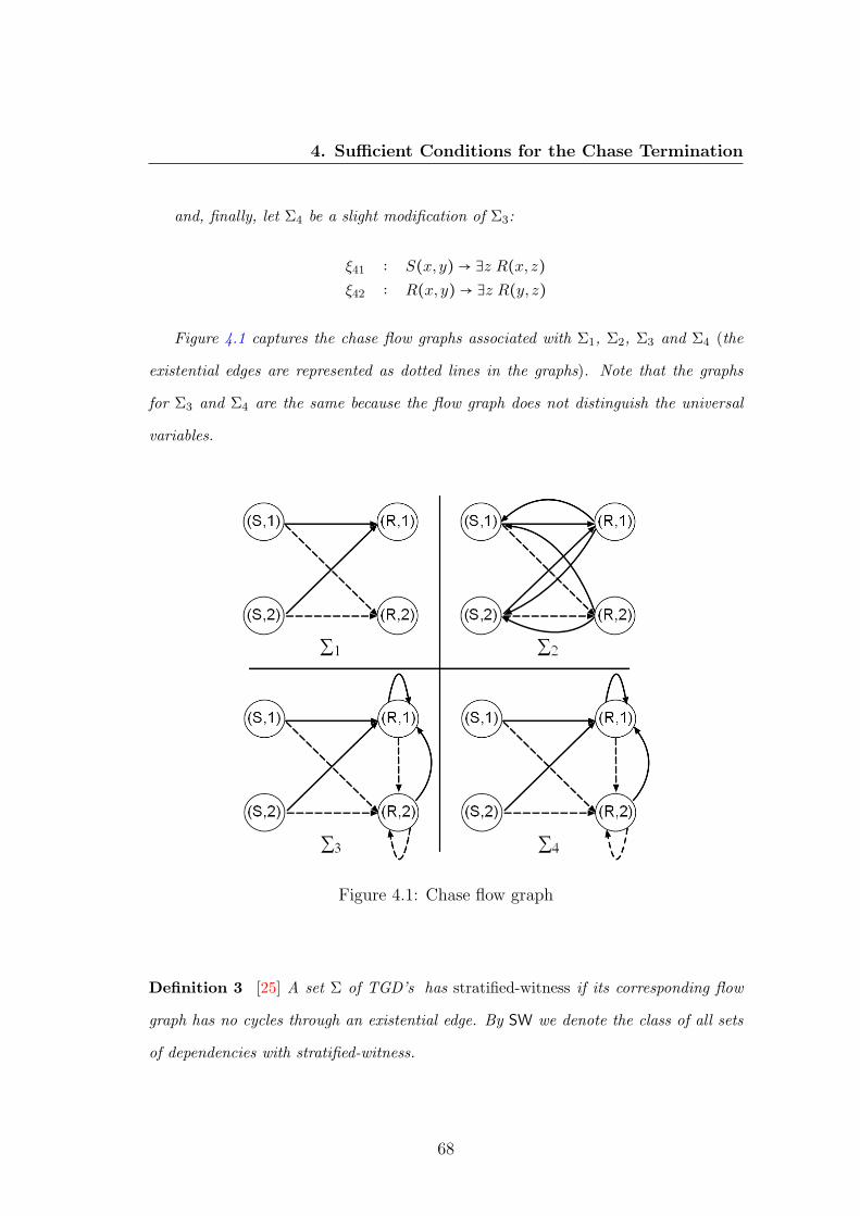
4. Sufficient Conditions for the Chase Termination
and, finally, let Σ4 be a slight modification of Σ3:
ξ41 ∶ S(x, y) → ∃z R(x, z)ξ42 ∶ R(x, y) → ∃z R(y, z)
Figure 4.1 captures the chase flow graphs associated with Σ1, Σ2, Σ3 and Σ4 (the
existential edges are represented as dotted lines in the graphs). Note that the graphs
for Σ3 and Σ4 are the same because the flow graph does not distinguish the universal
variables.
Figure 4.1: Chase flow graph
Definition 3 [25] A set Σ of TGD’s has stratified-witness if its corresponding flow
graph has no cycles through an existential edge. By SW we denote the class of all sets
of dependencies with stratified-witness.
68
4. Sufficient Conditions for the Chase Termination
Returning to example 12, only Σ1 has stratified-witness, all Σ2,Σ3 and Σ4 have
in their corresponding chase flow graph at least one cycle through an existential edge
(see Figure 4.1). The following theorem allows us to know that the standard chase
terminates for any set of TGD’s with stratified-witness.
Theorem 13 [25] If Σ ∈ TGD(R) such that Σ ∈SW, then Σ ∈ CTstd∀∀ . Even more, if i
denotes the maximum arity in R and k represents the number of existential edges in the
flow graph, then the standard-chase algorithm terminates for instance I in O(∣I ∣ik+1)
time.
From this theorem and the termination class hierarchy presented in Figure 3.7, it
follows that if Σ is a set of TGD’s with stratified-witness, then Σ ensures termination
on all instances also for the core chase and restricted-chase algorithms. In the following
section we will extend this result by showing that there exists a larger class of TGD’s
that guarantees the termination on all instances for the oblivious case following that
any set of TGD’s with stratified-witness are also in CTobl∀∀ and CTsobl
∀∀ .
4.3 Rich Acyclicity
The class of richly acyclic set of dependencies was introduced by Hernich and Schweikardt
in [47] in a different context. We will show here that any set of dependencies from this
new class ensures the oblivious-chase algorithm termination for all input instances.
Definition 4 [47] Let Σ be a set of TGD’s over schema R. The extended dependency
graph associated with Σ is a directed edge-labeled graph GEΣ = (V,E), such that each
vertex represents a position in R and ((R, i), (S, j)) ∈ E, if there exists a TGD ξ ∈ Σ
of the form ∀x, y α(x, y) → ∃z β(x, z), and if one of the following holds:
1. x ∈ x and x occurs in α on position (R, i) and in β on position (S, j). In this
case the edge is labeled as universal;
69

4. Sufficient Conditions for the Chase Termination
2. x ∈ x ∪ y and x occurs in α on position (R, i) and variable z ∈ z that occurs in β
on position (S, j). In this case the edge is labeled as existential.
Figure 4.2 illustrates the extended dependency graph for the sets of dependencies
specified in Example 12 (the existential edges are represented as dotted lines in the
graphs). Note that the extended dependency graph for Σ3 and Σ4 are not identical,
as they were for the flow graph. This is due to the fact that the extended dependency
graph distinguishes between the universally quantified variables.
Figure 4.2: Extended dependency graph
Definition 5 [47] A set Σ of TGD’s is said to be richly acyclic if the corresponding
extended dependency graph has no cycles through an existential edge. By RA we denote
the class of all richly acyclic sets of dependencies.
70

4. Sufficient Conditions for the Chase Termination
Returning to Example 12 from page 67, we may note that both Σ1 and Σ2 are
richly acyclic but that Σ3 and Σ4 are not. It is obvious that the problem of testing if
a given set of dependency Σ is in RA has polynomial complexity in the size of Σ. It
also follows directly from the definitions that SW⊂RA. For the strict inclusion part see
Σ2 from the previous example.
The following theorem shows that rich acyclicity implies oblivious-chase algorithm
termination on all instances in polynomial time in the size of the input instance.
Theorem 14 RA⊂ CTobl∀∀ and for any Σ ∈RA and any instance I there is a polynomial
in the size of I that bounds the execution time of the oblivious-chase algorithm with I
and Σ.
Proof: The proof of this theorem uses some of the notions introduced in the following
section, therefore the proof will be detailed in the next section at page 75∎
From this theorem and the class hierarchy illustrated in Figure 3.7, it follows that
if Σ is a richly acyclic set of dependencies, then Σ ensures termination on all instances
for all chase variations presented in Section 3.1.3.
4.4 Weak Acyclicity
Fagin et al. [27] introduced the class of weakly acyclic dependencies as a class that
ensures termination of the standard-chase algorithm on all execution branches for all
instances. This class of dependencies was initially introduced in the context of finding
universal solutions for the data exchange problem.
Definition 6 [27] Let Σ be a set of TGD’s over schema R. The dependency graph
associated with Σ is a directed edge-labeled graph GDΣ = (V,E), such that each vertex
71
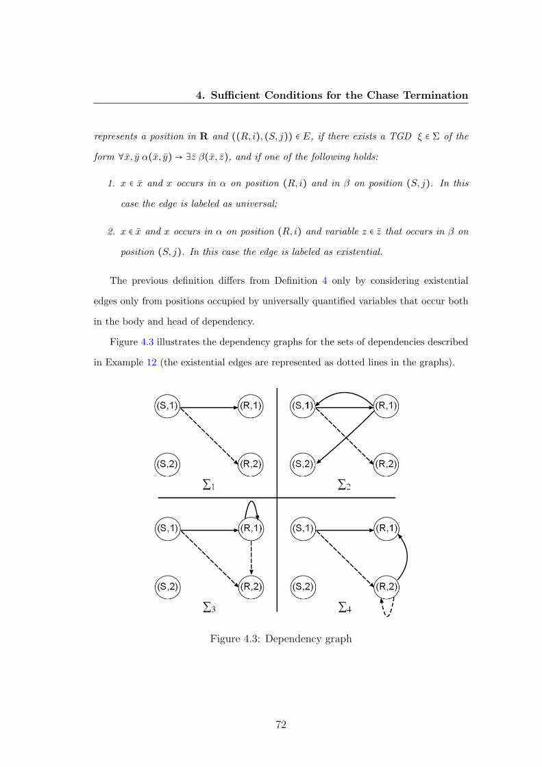
4. Sufficient Conditions for the Chase Termination
represents a position in R and ((R, i), (S, j)) ∈ E, if there exists a TGD ξ ∈ Σ of the
form ∀x, y α(x, y) → ∃z β(x, z), and if one of the following holds:
1. x ∈ x and x occurs in α on position (R, i) and in β on position (S, j). In this
case the edge is labeled as universal;
2. x ∈ x and x occurs in α on position (R, i) and variable z ∈ z that occurs in β on
position (S, j). In this case the edge is labeled as existential.
The previous definition differs from Definition 4 only by considering existential
edges only from positions occupied by universally quantified variables that occur both
in the body and head of dependency.
Figure 4.3 illustrates the dependency graphs for the sets of dependencies described
in Example 12 (the existential edges are represented as dotted lines in the graphs).
Figure 4.3: Dependency graph
72
4. Sufficient Conditions for the Chase Termination
Definition 7 [27] A set of TGD’s Σ is said to be weakly acyclic if the corresponding
dependency graph does not have any cycle going trough an existential edge. By WA we
denote the class of all weakly acyclic sets of dependencies.
Returning to Example 12 (see page 67), the first three sets of dependencies are
weakly acyclic, there are no edges through existentially labeled edges. The set Σ3 was
shown not to be richly acyclic but weakly acyclic, which gives us the strict inclusion
RA⊂WA. On the other hand, Gottlob and Nash noticed [34] that any weakly acyclic set
of dependency can be changed in a logically equivalent richly acyclic set of dependencies.
To obtain this, each tgd of the form α(x, y) → ∃z β(x, z), in case ∣y∣ > 0, is replaced
with the following two TGD’s:
α(x, y) → B(x) (4.1)
B(x) → ∃z β(x, z) (4.2)
The following theorem by Fagin et al. [27] shows that, for a weakly acyclic set of
dependencies, the standard-chase algorithm will terminate on all execution branches
for all instances in a polynomial number of steps, in the size of the input instance.
Theorem 15 [27] WA ⊂ CTstd∀∀ and for any Σ ∈ WA and any instance I there is a
polynomial, in the size of the input instance, that bounds the execution time of the
standard-chase algorithm with I and Σ.
Because of this theorem and the class hierarchy shown in Figure 3.7, it follows that
if Σ is a richly acyclic set of dependencies, then Σ ensures termination for standard,
restricted and core-chase algorithms. For the strict inclusion part from the previous
theorem, let us consider the following set of tgds Σ = {R(x,x) → ∃y R(y, x)}. Clearly,
Σ is not weakly acyclic. Still, for any instance I none of the tuples generated by
73

4. Sufficient Conditions for the Chase Termination
the head of the dependency will trigger the body. Thus the standard-chase algorithm
terminates on all branches for all input instances.
The following result extends the previous theorem by relating the WA class with
the CTsobl∀∀ and CTobl
∀∀ classes.
Proposition 12 WA⊂ CTsobl∀∀ and WA ∦ CTobl
∀∀ .
Proof: First it can be easily observed that if Σ ∈WA, then its semi-enrichment Σ ∈WA.
From this and Theorems 5 and 15, it directly follows that WA⊆ CTsobl∀∀ . For the strict
inclusion part, consider Σ1 = {S(y),R(x, y) → ∃z R(x, z)}. It is clear that Σ1 ∉WA , but
the standard-chase algorithm terminates on all branches for any instance I and Σ1. For
the second part, consider Σ2 = {R(x, y) → ∃z R(x, z)}, then clearly Σ2 ∈WAAnd from
Example 6 we have that Σ2 ∉ CTobl∀∀ . On the other hand, the previous set Σ1 ∈ CTobl
∀∀
and as shown Σ1 ∉WA. From this, it follows that WA ∦ CTobl∀∀ ∎
Lemma 1 Let Σ be a richly acyclic set of TGD’s then Σ, the enrichment of Σ, is a
weakly acyclic set of TGD’s.
Proof: Let Σ be a set of TGD’s with the corresponding extended dependency graph
GEΣ = (V E ,EE). Let Σ be the enrichment of Σ with the corresponding dependency
graph GDΣ= (V D,ED). We will show first that the graph GD
Σrestricted to the vertexes
V E is the same as GEΣ . For this, let us consider a tgd ξ ∈ Σ of the form:
∀x,∀y R1(x1, y1),R2(x2, y2), . . . ,Rn(xn, yn) → ∃z S1(x′1, z1), S2(x′2, z2), . . . , Sm(x′m, zn)
where x = ∪i∈[n]xi = ∪j∈[m]x′j , z = ∪i∈[m]zi and y = ∪i∈[n]yi. The corresponding enriched
dependency ξ belonging to Σ will have the following form:
∀x,∀y R1(x1, y1),R2(x2, y2), . . . ,Rn(xn, yn) →
∃z S1(x′1, z1), S2(x′2, z2), . . . , Sm(x′m, zn),H(x, y)
74
4. Sufficient Conditions for the Chase Termination
where H is a new relational symbol. Let us suppose that ξ creates the universal edge
((Ri, k), (Sj , l)) in the extended dependency graph GEΣ . From this it follows that the
same universal edge is also part of GDΣ
because both dependencies use the same set of
universal variables that occurs in the same positions in both ξ and ξ. Let us now suppose
that ξ creates the existential edge ((Ri, k), (Sj , l)) in the extended dependency graph
GEΣ . This means that on position (Ri, k) occurs a variable either from x or y and that
on position (Sj , l) from the head occurs a variable from z. Clearly, ((Ri, k), (Sj , l))
is also an existential edge in the dependency graph GDΣ
. The only edges in GDΣ
not
occurring in GEΣ are the universal edges oriented to the positions over relation H. As
relation H does not appear in the body of any dependency in Σ, it follows that there
can’t be any cycle in GDΣ
through a position over H. But this means that any cycle in
GEΣ is also a cycle in GD
Σand vice versa. From this it directly follows that Σ is a richly
acyclic set of TGD’s if and only if Σ is a weakly acyclic set of TGD’s∎
Now we are ready to prove Theorem 14 stated at page 71.
Theorem 14 RA⊂ CTobl∀∀ and for any Σ ∈RA and any instance I there is a polynomial,
in the size of the instance I, that bounds the execution time of the oblivious-chase
algorithm with I and Σ.
Proof: Let Σ be a richly acyclic set of TGD’s. From the previous theorem we have that
Σ is a weakly acyclic set of TGD’s. On the other hand, from Theorem 15 it follows that
the standard-chase procedure terminates with Σ for any instance I, that is Σ ∈ CTstd∀∀ .
From this and Theorem 3 follows that Σ ∈ CTobl∀∀ . For the strict part inclusion it is easy
to verify that the dependency Σ = {R(x,x) → ∃y R(x, y), T (x)} ensures the oblivious
chase termination for any input instance, that is Σ ∈ CTobl∀∀ , but Σ ∉RA. For the second
part of the theorem, let I and let kI be the polynomial that bounds the execution time
for the standard chase on input Σ and I, as given by Theorem 15. But from the proof of
75

4. Sufficient Conditions for the Chase Termination
Theorem 3 we have that the number of steps executed by the standard-chase algorithm
on input Σ and I is the same with the number of steps executed by the oblivious-chase
algorithm on input Σ and I. Thus kI is also a polynomial that bounds the execution
time for the oblivious chase on input Σ and I∎
4.5 Safe Dependencies
Meier, Schmidt and Lausen [61] observed that the weak acyclicity condition restricts
also tgds that introduce new nulls that may not create infinite standard-chase se-
quences.
Example 13 Let us consider an example from [61] with Σ containing only one depen-
dency TGD:
ξ ∶ R(x, y, z), S(y) → ∃w R(y,w, x)
Figure 4.4 represents the dependency graph corresponding to Σ. As it can be seen
in the figure, the dependency graph contains a cycle going through an existential edge.
Thus Σ is not weakly acyclic. On the other hand, the newly created null in position
(R,2) may create new null values only if the same null also appears in position (S,1).
Based on the given dependency, new nulls cannot be generated in position (S,1). Thus
this dependency can not cyclically create new nulls.
In order to be able to capture the type of dependencies presented in the previous
example, Meier et al. observed that we need to change the dependency graph such that
it does not contain as vertexes all the position in the schema, but only the ones that
may contribute to an infinite cycle, that is positions in which new null values can occur.
Before introducing the notion of safe dependencies, let us first present the definition
of the affected position introduced by Cali et al. in [16].
76

4. Sufficient Conditions for the Chase Termination
Figure 4.4: Dependency graph with cycles through existential labeled edges
Definition 8 [16] The affected positions associated with a set of TGD’s Σ is the set
aff(Σ) defined recursively as follows. Position (R, i) ∈ aff(Σ) if: ξ ∈ Σ, then
1. if an existential variable appears in position (R, i) in ξ, or;
2. if universally quantified variable x appears in position (R, i) in the head of some
dependency ξ ∈ Σ and x occurs only in affected positions in the body of ξ.
Returning to Example 13, it can be easily noted that aff(Σ) = {(R,2)}. Similarly
to the dependency graph, the propagation graph is defined as:
Definition 9 [61] Let Σ be a set of TGD’s . The propagation graph associated with
Σ is a directed edge labeled graph GPΣ = (aff(Σ),E), where ((R, i), (S, j)) ∈ E if there
exists a dependency ξ ∈ Σ of the form ∀x, y α(x, y) → ∃z β(x, z), and there exists a
variable x ∈ x that occurs in the body of ξ in position (R, i), such that x occurs only in
affected positions in body of ξ and either
• x occurs in position (S, j) in β, or
77

4. Sufficient Conditions for the Chase Termination
• there exists a variable z ∈ z in position (S, j) in β.
In the first case, the edge is labeled as universal and, in the second case, the edge is
labeled as existential.
Considering again Example 13, as shown, the only affected position is (R,2). On
the other hand, only the universally quantified variable y occurs in this affect position
in the body of the dependency, variable that occurs in a non-affected position (R,1) in
the head of the dependency.
Example 14 [61] Consider Σ consisting of the following two TGD’s:
ξ1 ∶ S(x),R(x, y) → R(y, x)
ξ2 ∶ S(x),R(x, y) → ∃z R(y, z),R(z, x)
asserting that all nodes in S have cycles of length 2 (ξ1) and 3 (ξ2). The set of affected
positions in this case is aff(Σ) = {(R,1), (R,2)}. Figure 4.5 shows the propagation
graph corresponding to Σ (the dotted lines represent the existential edges).
Figure 4.5: Propagation graph
78

4. Sufficient Conditions for the Chase Termination
Definition 10 [61] A set Σ of TGD’s is called safe if its propagation graph GPΣ does
not have a cycle going trough an existential edge. By SD to be the class of all safe
dependency sets.
Using this definition, it follows that the set of dependencies from Example 13 is
safe as the corresponding propagation graph contains a single vertex and no edges.
On the other hand, the dependencies from Example 14 are not safe. Note the cycle
through an existentially labeled edge in Figure 4.5. It may be also noted that the set
of dependencies from Example 14 guarantees the standard-chase termination for all
instances.
Theorem 16 [61] SD⊂ CTstd∀∀ and for any Σ ∈SD and any instance I there is a poly-
nomial, in the size of I, that bounds the execution time of the oblivious-chase algorithm
with I and Σ.
For the strict inclusion part of the previous theorem, consider that the set of de-
pendencies from Example 14 is in CTstd∀∀ but it is not safe. Meier et al. [61] also proved
that WA⊂SD. However, this does not hold with the propagation graph defined in their
paper. For the strict inclusion between the classes WA and SD consider the set of
dependencies from Example 13 which is safe but not weakly acyclic. The following
proposition extends the previous result by showing that the safe dependencies also en-
sure the semi-oblivious-chase termination for all instances but do not guarantee the
oblivious-chase termination on all instances.
Proposition 13 SD⊂ CTsobl∀∀ and SD ∦ CTobl
∀∀ .
Proof: First it can be observed that if Σ ∈SD, then its semi-enrichment Σ ∈SD, as the
corresponding propagation graphs restricted to the positions over Σ are the same, and
79

4. Sufficient Conditions for the Chase Termination
the new relations introduced in Σ do not induce any cycle in the corresponding prop-
agation graph. From this and Theorems 5 and 16 it directly follows that SD⊆ CTsobl∀∀ .
For the strict inclusion part, consider Σ1 = {R(x,x) → ∃y R(x, y)}. It is obvious that
Σ1 ∉SD , but the semi-oblivious-chase algorithm terminates for any instance I and Σ1.
For the second part, consider Σ2 = {R(x, y) → ∃z R(x, z)}. Clearly Σ2 ∈SD and from
Example 6 we have that Σ2 ∉ CTobl∀∀ . Let us not forget that the previous set Σ1 ∈ CTobl
∀∀
and, as shown, Σ1 ∉SD. The consequence is that SD ∦ CTobl∀∀ ∎
4.6 Super Weak Acyclicity
The following class of dependencies properly extends the class of safe dependencies
and consequently the class of weakly acyclic, richly acyclic dependencies and the class
of dependencies with stratified witness. This class of dependencies, introduced by
Marnette [59], beside omitting the nulls that can’t generate infinite chase sequences, as
in the case of safe dependencies, also takes into account the repeating variables. For
a uniform presentation of the dependency classes, we will slightly change the notation
used in [59]
We assume that the set of dependencies Σ has distinct variable names in each
dependency. We also assume that there exists a total order between the atoms in
each dependency. With this, we can now define the notion of atom position to be a
triple (ξ,R, i), where ξ ∈ Σ, R is a relation name that occurs in ξ, i ∈ [n], where n is
the maximum number of occurrences of R in ξ, given by the total order between the
atoms in the dependency. Clearly each atom position uniquely identifies an atom in
Σ. Similarly to the notion of position, a place can be defined as a pair ((ξ,R, i), k),
where (ξ,R, i) is an atom position and k ∈ [arity(R)]. Intuitively, the place identifies
the variable that appears in the k-th position in the atom given by the atom position
(ξ,R, i).
80
4. Sufficient Conditions for the Chase Termination
Let V ar(ξ) define the set of all variables that occur in dependency ξ ∈ Σ. As men-
tioned, for any two distinct dependencies ξ1 and ξ2 in Σ, we have V ar(ξ1)∩V ar(ξ2) = ∅.
The mapping V ar is extended to a set of dependencies Σ as V ar(Σ) = ∪ξ∈Σ V ar(ξ).
Similarly, we define mappings V ar∃ and V ar∀ that map each dependency ξ to the set
of existentially marked variables in ξ and to the universally quantified variables in ξ re-
spectively. Clearly, for each dependency ξ, V ar∃(ξ) and V ar∀(ξ) represent a partition
of V ar(ξ).
Given a TGD ξ and y ∈ V ar∃(ξ), Out(ξ, y) is defined to be the set of places in the
head of ξ where y occurs. Given a set a TGD ξ and x ∈ V ar∀(ξ), In(ξ, x) is defined to
be the set of places in the body of ξ where x occurs.
A substitution for Σ is a function θ with Dom(θ) = ΔV and Im(θ) = ΔC such that
for any x ∈ V ar∃(Σ) there is no variable y ∈ V ar(Σ) with x ≠ y such that θ(x) = θ(y).
Given a substitution θ for Σ and an atom (ξ,R, i) from Σ, the new atom resulting by
replacing each variable x in (ξ,R, i) with θ(x) is denoted by θ(ξ,R, i). Two atoms,
(ξ1,R, i1) and (ξ2,R, i2), are said to be unifiable if there exist two substitutions θ1
and θ2 for Σ such that θ1(ξ1,R, i1) = θ2(ξ2,R, i2). Two places p1 = ((ξ1,R, i1), k1) and
p2 = ((ξ2,R, i2), k2) are said to be unifiable if k1 = k2 and (ξ1,R, i1) is unifiable with
(ξ2,R, i2). By p1 ∼ p2 we denote that p1 and p2 are unifiable. Let us define ΓΣ to be
a function that maps each variable x to the set of places where x occurs in Σ. The
function ΓHΣ maps each variable x to the set of places from the head of some dependency
where x occurs. Similarly, the function ΓBΣ maps each variable x to the set of places
from the body of some dependency where x occurs.
For a better understanding of the previous notions, consider the example:
Example 15 [70] Let Σ contain two dependencies:ξ1 ∶ R(x) → ∃y, z S(x, y, z)
ξ2 ∶ S(v,w,w) → R(w)
81

4. Sufficient Conditions for the Chase Termination
The following are the atom positions for Σ:
• (ξ1,R,1), corresponding to atom R(x);
• (ξ1, S,1), corresponding to atom S(x, y, z);
• (ξ2, S,1), corresponding to atom S(v,w,w);
• (ξ2,R,1), corresponding to atom R(w).
For this setting we have the set V ar∀(Σ) = {x, v,w}, V ar∃(Σ) = {y, z} and the set
V ar∀(Σ) = V ar∀(Σ) ∪ V ar∃(Σ). Clearly (ξ1,R,1) is unifiable with (ξ2,R,1), consider
unifier θ1 = {x/a} and θ2 = {w/a}. On the other hand, atom positions (ξ1, S,1) and
(ξ2, S,1) are not unifiable as there do not exist two unifiers θ1 and θ2 for the atoms
S(x, y, z) and S(v,w,w) such that the existential variables y, z each are mapped to a
new constant. From this we have that ((ξ1,R,1),1) ∼ ((ξ2,R,1),1). For variable x,
we have the sets ΓΣ(x) = {((ξ1,R,1),1), ((ξ1, S,1),1)}, ΓBΣ(x) = {((ξ1,R,1),1)} and
ΓHΣ (x) = {((ξ1, S,1),1)}.
Given two sets of places P and Q, we denote P ⊑ Q if for all p ∈ P if p ∼ q, then
q ∈ Q. The mapping Move(Σ,Q) is defined to return the smallest set of places P ,
with Q ⊆ P and for all variables x that occur in a body of some dependency ξ ∈ Σ
if ΓBΣ(x) ⊑ P then ΓH
Σ (x) ⊆ P . Intuitively, the Move(Σ,Q) returns the smallest set of
places such that the values generated in those places by chasing some tuples that contain
the places in Q are dependent on the values in tuples in places Q. Returning to the
dependencies from the previous example and considering the place p1 = (ξ2,R,1),1),
with this place we have only place p2 = (ξ1,R,1),1) such that p1 ∼ p2. Also we have
ΓBΣ(x) = {p2} and ΓH
Σ (x) = {p3}, where p3 = ((ξ1, S,1),1). From this it follows that
Move(Σ,{p1}) = {p1, p2, p3}.
Definition 11 [59] Given Σ a set of TGD’s and ξ1, ξ2 ∈ Σ, we say ξ1 triggers ξ2 in Σ,
and it is denoted with ξ1 ↝Σ ξ2, iff there exists a variable y ∈ V ar∃(ξ1) and a variable
x ∈ V ar∀(ξ2) occurring in both the body and the head of ξ2 such that:
82
4. Sufficient Conditions for the Chase Termination
In(ξ2, x) ⊑ Move(Σ,Out(ξ1, y))
Definition 12 [59] A set of TGD’s Σ is said to be super-weakly acyclic iff the trigger
relation ↝Σ is acyclic. By SwA we denote the set of all super-weakly acyclic depen-
dencies.
Example 16 Consider Σ = {ξ1, ξ2} as in Example 15. The place ((ξ1, S,1),1) is not
unifiable with ((ξ2, S,1),1) and In(ξ2,w) /⊑ Move(Σ,Out(ξ1, y)), thus ξ1 /↝Σ ξ2. Simi-
larly, ξ2 does not contain any existential variables and so it follows that ξ2 /↝Σ ξ1. As
both dependencies do not share common relation names in the head and the body, it
follows that ξ1 /↝Σ ξ1 and ξ2 /↝Σ ξ2. That is the relation ↝Σ does not induce any cycle,
following that Σ is super-weakly acyclic. Moreover, it can be seen that Σ ∉SD, as be-
tween the affected positions (R,1) and (S,2) there exists a cycle through an existential
edge in the corresponding propagation graph.
Marnette [59] showed that the membership problem Is Σ ∈SwA? has a polynomial
complexity in the size of Σ. The following theorem proves that super-weakly acyclicity
is a sufficient condition for the semi-oblivious-chase termination on all instances.
Theorem 17 SwA⊂ CTstd∀∀ and for any Σ ∈SwA and any instance I there exists a
polynomial, in size of I, that bounds the execution time of the semi-oblivious-chase
algorithm with I and Σ.
Proof: It follows directly from Theorem 2 and Theorem 5 in [59].
Proposition 14 [59] WA⊂SwA.
83

4. Sufficient Conditions for the Chase Termination
Later, Spezzano and Greco [70] also showed that SD⊂SwA, that is the super-weak
acyclic dependencies properly contain all safe dependencies. A nice property of the
class SwA is that it is closed in adding atoms in the body of dependencies, thus given
a set of TGD’s Σ ∈SwA, then any set of dependencies Σ′, obtained from Σ by adding
new atoms in the body of any dependencies, remains super-weakly acyclic.
The previous theorem together with Proposition 7 give us the following corollary:
Corollary 5 Let Σ ∈SwA and let I be an instance. Then there exists a polynomial, in
the size of I, that bounds the length of every standard-chase sequence of I and Σ.
The following proposition shows that super-weak acyclicity class is incomparable
with the class of dependencies that ensures the oblivious-chase termination on all in-
stances.
Proposition 15 SwA ∦ CTobl∀∀ .
Proof: Let us consider Σ1 = {R(x, y) → ∃z R(x, z)}. It is clear that Σ1 ∈SwA but
the oblivious-chase algorithm does not terminate with input I = {R(a, b)} and Σ1.
Let us now consider Σ2 = {S(x),R(x, y) → ∃z R(y, z)} and denote the dependency in
Σ2 by ξ. With this we have In(ξ, x) = {((ξ,R,1),2)}, Out(ξ, z) = {((ξ,R,2),2)} and
Move(Σ,Out(ξ, z)) = {((ξ,R,2),2), ((ξ,R,1),2)}, that is In(ξ, x) ⊑ Move(Σ,Out(ξ, z)).
Thus, based on Definition 11, ξ ↝Σ2 ξ following that Σ2 ∉SwA. On the other hand it
can be observed that the oblivious-chase algorithm terminates for any instance I. This
is because the dependency may be obliviously fired only if the first position in R does
not contain a null value∎
This concludes that the super-weakly acyclic class of dependencies ensures that the
standard, semi-oblivious, restricted and core-chase algorithms terminate for all input
instances.
84

4. Sufficient Conditions for the Chase Termination
4.7 Stratification
The stratified model of dependencies was introduced by Deutsch et al. in [23]. This
class relaxes the condition imposed by weak acyclicity by stratifying the dependencies
and checking for weak acyclicity on each of these strata.
Before presenting the notion of stratification let us introduce a new notation. Given
ξ a tgd of the form:
α(x, y) → ∃z β(x, z)
and a vector a = (a1, . . . , an, an+1, . . . , an+m) of constants where n = ∣x∣ and m = ∣y∣, by
ξ(a) we denote the following formula without any universally quantified variables:
α((a1, . . . , an), (an+1, . . . , an+m)) → ∃z β((a1, . . . , an), z)
Definition 13 [23] Let ξ1 and ξ2 be two TGD’s , we write ξ1 ≺ ξ2, if there exist in-
stances I, J and vector a ⊆ dom(J), such that
1. I ⊧ ξ2(a), and
2. there exists a standard trigger (ξ1, h), such that I(ξ1,h)���→ J , and
3. J /⊧ ξ2(a).
Example 17 Consider the following two TGD’s:
ξ1 ∶ ∀x, y R(x, y) → S(x)
ξ2 ∶ ∀x, y S(x) → R(x,x)
For the instance I = {R(a, b)} and a = (a) we have that I ⊧ ξ2(a); and for homo-
morphism h = {X/a, Y /b} we have I(ξ1,h)���→ J , where J = {R(a, b), S(a)}. Because
J /⊧ ξ2(a), it follows that ξ1 ≺ ξ2. On the other hand, ξ2 /≺ ξ1 because for any vector of
85

4. Sufficient Conditions for the Chase Termination
constants b = (a, b) and instance I such that I ⊧ ξ1(b) and for any trigger (ξ, h) such
that I(ξ2,h)���→ J , it follows that J ⊧ ξ1(b).
Given two TGD’s ξ1 and ξ2, the decision problem Is ξ1 ≺ ξ2? is known to be in NP
[23]. To the best of our knowledge there yet is no result proving the lower bound of
this problem.
Given a set of TGD’s Σ, the chase graph associated with Σ is a directed graph
GCΣ = (V,E), where V = Σ and (ξ1, ξ2) ∈ E iff ξ1 ≺ ξ2.
Definition 14 [23] A set of TGD’s Σ is said to be stratified if the set of dependencies
in every cycle in the corresponding chase graph is weakly acyclic. The class of all
stratified sets of dependencies is denoted with Str.
In [61] it is shown that stratification does not guarantee that the standard-chase
algorithm terminates on all execution branches for all instances (see example bellow).
Example 18 [61] Consider the following set of TGD’s:
ξ1 ∶ R(x) → S(x,x)
ξ2 ∶ S(x, y) → ∃z T (y, z)
ξ3 ∶ S(x, y) → T (x, y), T (y, z)
ξ4 ∶ T (x, y), T (x, z), T (z, x) → R(y)
The set Σ = {ξ1, ξ2, ξ3, ξ4} is stratified since ξ1 ≺ ξ2, ξ1 ≺ ξ3 ≺ ξ4 ≺ ξ1; and the set
{ξ1, ξ3, ξ4} is weakly acyclic. Let us consider instance I = {R(a)}. The standard-chase
algorithm that triggers repeatedly dependencies ξ1, ξ2, ξ3 and ξ4 never terminates. On
the other hand, the chase sequence that never triggers ξ2 terminates.
Since the stratification does not ensure termination for the standard chase for all
instances, the following question arises: does the stratification sometimes guarantee
86

4. Sufficient Conditions for the Chase Termination
termination of the standard-chase algorithm on some branches for all instances? The
answer to this question is given by the following theorem:
Theorem 18 Str⊂ CTstd∀∃ and Str ∦ CTstd
∀∀
Proof: The first part of the theorem is proved in [61]. For the strict inclusion part,
consider Σ1 = {ξ1 ∶ S(x),R(x, y) → ∃z R(y, z)}. Of course, there is no doubt that
Σ1 ∈ CTstd∀∀ ⊂ CTstd
∀∃ . On the other hand, ξ1 ≺ ξ1; as for instance I = {R(b, a), S(a), S(b)}
we have I ⊧ ξ(a, b), I(ξ,h)���→ J , where h = {X/a, Y /b}, J = I∪{R(a,Z),} and J /⊧ ξ(a,Z),
thus Σ is not stratified. Example 18 shows a set of TGD’s Σ such that Σ ∈Str but
Σ ∉ CTstd∀∀ ∎
From the previous theorem and Theorem 10 it follows that the core-chase algorithm
terminates for all instances over a set of stratified TGD’s.
Meier et al. [61] improved the stratification notion in order to ensure also that the
standard-chase algorithm terminates on all execution branches for all instances. For
this they changed the ≺ relation as follows:
Definition 15 [61] Let ξ1 and ξ2 be two TGD’s. We write ξ1 ≺c ξ2, if there exist
instances I, J and vector a ⊆ dom(I), such that
1. I ⊧ ξ2(a), and
2. there exists an oblivious trigger (ξ1, h), such that I∗(ξ1,h)����→ J , and
3. J /⊧ ξ2(a).
Given a set of TGD’s Σ, the c-chase graph associated with Σ is a directed graph
GCCc = (V,E). With V = Σ and (ξ1, ξ2) ∈ E iff ξ1 ≺c ξ2. A set of TGD’s Σ is said to
be c-stratified if the set of dependencies in every cycle in the c-chase graph is weakly
acyclic. The set of all c-stratified dependencies is denoted by CStr.
87
4. Sufficient Conditions for the Chase Termination
Theorem 19 [61] CStr⊂ CTstd∀∀ and for any Σ ∈CStr and any instance I there exists
a polynomial, in the size of I, that bounds the execution time of the standard-chase
algorithm with I and Σ.
The previous theorem showed that CStr ensures termination for the standard chase.
We can now extend this result by showing that CStr ensures the termination of the
semi-oblivious-chase algorithm.
Theorem 20 CStr⊂ CTsobl∀∀ and CStr ∦ CTobl
∀∀ .
Proof: Let us first prove that CStr⊆ CTsobl∀∀ . For this, consider a set of TGD’s Σ ∈CStr.
Let us now consider the semi-enrichment Σ. We will show that if ξ1 ≺c ξ2 for ξ1, ξ2 ∈ Σ,
then ξ1 ≺c ξ2 for ξ1, ξ2 ∈ Σ. Let I, J be two instances and a and b be the vectors
such that I ⊧ ξ2(a), I∗(ξ1,h)����→ J for some homomorphism h and J /⊧ ξ2(b). Consider
instance I ′ = I ∪ {H2(a)}, where H2 is the relation symbol introduced by the semi-
enrichment for ξ2. By abusing the notation by H2(a) we denote the tuple over H2 that
contains the values from a that occurs in both the body and the head of ξ2. Let us also
consider instance J ′ = J ∪ {H1(h(x))}, where H1 is the relational symbol introduced
by the semi-enrichment for ξ1 and x is the vector of universally quantified variables
that occurs both in the body and the head of ξ1. It is easy to observe that I ′ ⊧ ξ2(a),
I ′∗(ξ1,h)����→ J ′ for homomorphism h, and J ′ /⊧ ξ2(b), thus ξ1 ≺c ξ2. From this it follows
that Σ has an isomorphic c-chase graph with Σ (note that the same result holds for
the enrichment Σ). Also, we know that the dependency graphs corresponding to Σ and
Σ are isomorphic as well (this property does not hold for the enrichment Σ). Thus
Σ ∈CStr implies that Σ ∈CStr. Because we know from Theorem 19 that CStr ∈ CTstd∀∀ ,
it follows that Σ ∈ CTstd∀∀ . On the other hand, Theorem 5 shows that if Σ ∈ CTstd
∀∀ then
Σ ∈ CTsobl∀∀ . Thus it follows that CStr⊆ CTsobl
∀∀ . For the strict part of the inclusion,
consider Σ1 = {ξ1 ∶ S(x),R(x, y) → ∃z R(y, z)}. Similarly to the proof from 18, it
88

4. Sufficient Conditions for the Chase Termination
can be shown that Σ1 ∉CStr, but Σ1 ∈ CTobl∀∀ ⊂ CTsobl
∀∀ . It remained to show only
that CStr/⊆ CTobl∀∀ . For this consider Σ2 = {ξ ∶ R(x, y) → ∃z R(y, z)}. For this set of
dependencies we know from the previous proofs that Σ2 ∈WA⊂CStr and Σ2 ∉ CTobl∀∀ ∎
The problem of checking if a set of Σ is in Str (or CStr) is known to be in coNP [23]
([61]). To the best of our knowledge the lower bound is still an open problem.
The following Theorem gives the relationship between CStr and the classes WA,
SD and SwA.
Theorem 21 WA ⊂ CStr, SD ∦ CStr [61] and SwA ∦ CStr [70]
4.8 Inductively Restricted Dependencies
Another class of dependencies that guarantees the standard-chase termination is the
inductively restricted set of dependencies. Note that the stratification method lifts
the weakly acyclic class of dependencies to the class of c-stratified dependencies. The
inductively restricted class generalizes the stratification method while still keeping the
termination property for the standard-chase algorithm. This generalization is done
using the so-called restriction systems [61]. With the help of the restriction systems,
Meier et al. [61] define the new sufficient condition called inductive restriction which
guarantees the standard-chase algorithm termination for all instances on all branches.
From this condition a new hierarchy of classes of dependencies is revealed with the
same termination property, called the T-hierarchy. Note that the inductive restriction
condition presented here is given from the erratum [62] and not from [61], where the
presented condition, as mentioned in the erratum, does not guarantee the standard-
chase termination on all execution branches for all instances.
89
4. Sufficient Conditions for the Chase Termination
Let Σ be a set of TGD’s, I an instance and A a set of null, A ⊆ ΔN. The set of
all positions (R, i) such that there exists a tuple in I which contains a null from A in
position (R, i) and which is denoted by null-pos(A, I) .
Similarly with ”≺” relation for the stratified dependencies, the binary relation ”≺P”
is defined for the inductive restriction condition for P a set of positions.
Definition 16 [61] Let Σ be a set of TGD’s and P a set of positions from Σ. Let ξ1,
ξ2 be two dependencies in Σ. It is said that ξ1 ≺P ξ2, if there exist instances I, J and
vector a such that:
1. I ⊧ ξ2(a), and
2. there exists an oblivious trigger (ξ1, h), such that I∗(ξ1,h)����→ J , for a homomor-
phism h, and
3. J /⊧ ξ2(a), and
4. there exists X ∈ a ∩ΔN in head(ξ2(a)) such that null-pos({X}, I) ⊆ P .
Example 19 Consider Σ containing a single TGD ξ ∶ R(x, y) → ∃z R(y, z). Example
3 showed that there exists an instance I such that standard-chase algorithm does not ter-
minate for I and Σ. Consider I = {R(a, b)} and vector a = (b,X1). It is easy to see that
condition 1 from the previous definition is satisfied, thus I ⊧ ξ(a) as there is no homo-
morphism from body(ξ) to I. On the other hand, for homomorphism h = {X/b, Y /X1},
we have I∗(ξ1,h)����→ J , where J = {R(a, b),R(b,X)}, thus the second condition from the
previous definition is fulfilled as well. The third condition is also met as J /⊧ ξ(a). The
4th condition is also satisfied. For this consider the null X1 ∈ a, then we have ξ(a)
representing formula R(a,X1) → ∃zR(X1, z). Thus, X1 occurs in head(ξ(a)). On the
other hand, null-pos({X1}, I) = ∅, because instance I does not contain any nulls, that
is for any set P , null-pos({X}, I) ⊆ P . Thus ξ ≺P ξ, for any set P of positions.
90

4. Sufficient Conditions for the Chase Termination
Definition 17 [61] Let P be a set of positions and ξ a TGD. aff-cl(ξ,P ) is the set of
positions (R, i) from the head of ξ such that:
1. for all x ∈ V ar∀(ξ), with x occurs in (R, i), x occurs in the body of ξ only in
positions from P , or
2. position (R, i) contains a variable x ∈ V ar∃(ξ).
Considering the dependency from Example 19, we have aff-cl(ξ,P ) = {(R,1), (R,2)},
where P = {(R,2)}. Given a set of dependencies Σ, by pos(Σ) is denoted the set of all
positions in Σ.
Definition 18 [61] A 2-restriction system is a pair (G(Σ), P ), where G(Σ) is a di-
rected graph (Σ,E) and P ⊆ pos(Σ) such that:
1. for all (ξ1, ξ2) ∈ E, aff-cl(ξ1, P ) ∩ pos(Σ) ⊆ P and aff-cl(ξ2, P ) ∩ pos(Σ) ⊆ P ,
2. for all ξ1 ≺P ξ2, (ξ1, ξ2) ∈ P .
A 2-restriction system is minimal if it is obtained from ((Σ,∅),∅) by a repeated
application of constraints 1 and 2, from the previous definition, such that P is extended
only by those positions that are required to satisfy condition 1. Let us denote part(Σ,2)
to contain the sets of all strongly connected components in minimal 2-restriction system.
Example 20 Considering Σ from Example 19, the minimal 2-restriction system is
computed as follows. Consider pair (({ξ},∅),∅). We previously showed that ξ ≺P ξ,
for any set of positions P . And by particularization we have ξ ≺∅ ξ. Thus, we add
edge (ξ, ξ) to E. Let us remember that the condition 1 from definition 18 stipulates
that aff-cl(ξ,∅) = {(R,2)}. Therefore, we add position (R,2) to P . By repeating this
process with P = {(R,2)}, we also add to P the position (R,1). Thus, the minimal
2-restriction system is ((Σ,{(ξ, ξ)),{(R,1), (R,2)}}). The only connected component
in this restriction system is {ξ}.
91
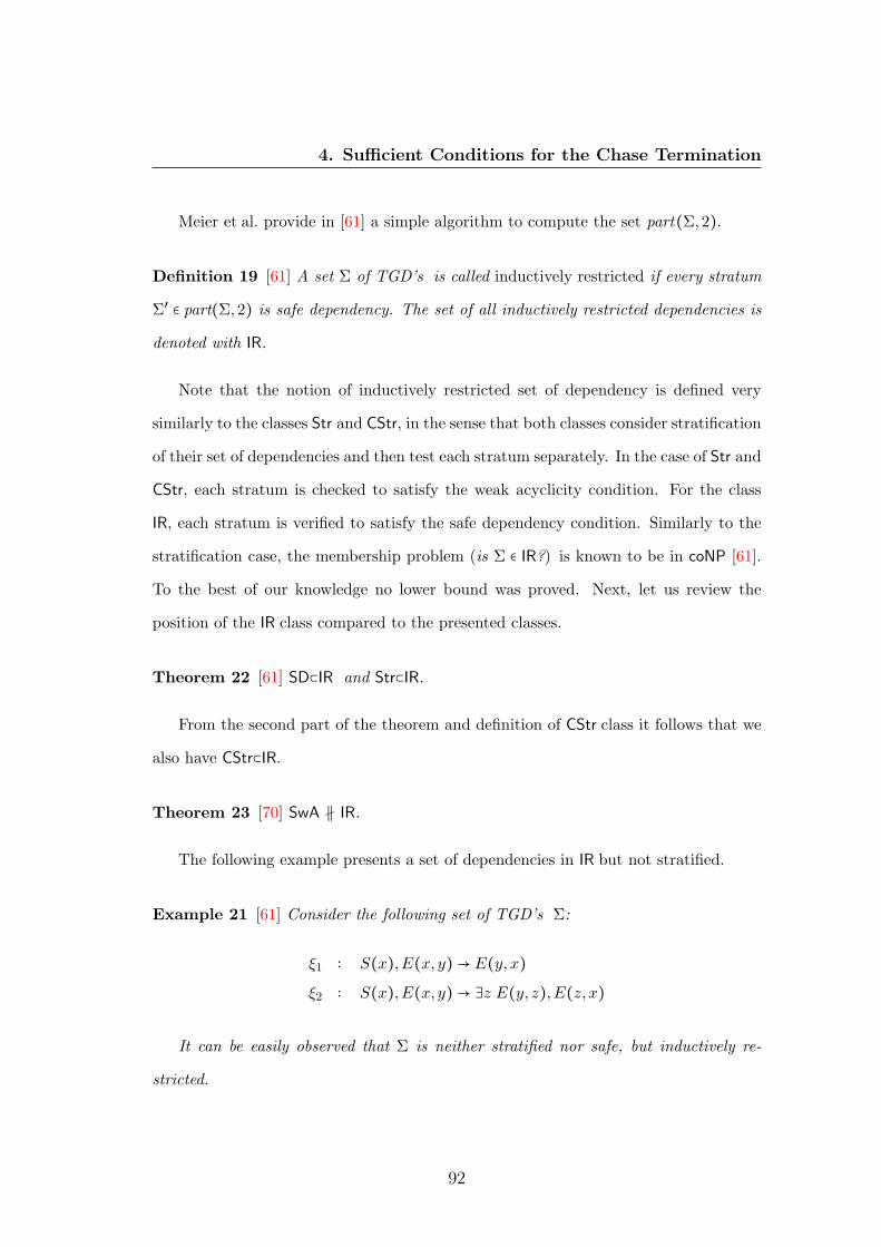
4. Sufficient Conditions for the Chase Termination
Meier et al. provide in [61] a simple algorithm to compute the set part(Σ,2).
Definition 19 [61] A set Σ of TGD’s is called inductively restricted if every stratum
Σ′ ∈ part(Σ,2) is safe dependency. The set of all inductively restricted dependencies is
denoted with IR.
Note that the notion of inductively restricted set of dependency is defined very
similarly to the classes Str and CStr, in the sense that both classes consider stratification
of their set of dependencies and then test each stratum separately. In the case of Str and
CStr, each stratum is checked to satisfy the weak acyclicity condition. For the class
IR, each stratum is verified to satisfy the safe dependency condition. Similarly to the
stratification case, the membership problem (is Σ ∈ IR?) is known to be in coNP [61].
To the best of our knowledge no lower bound was proved. Next, let us review the
position of the IR class compared to the presented classes.
Theorem 22 [61] SD⊂IR and Str⊂IR.
From the second part of the theorem and definition of CStr class it follows that we
also have CStr⊂IR.
Theorem 23 [70] SwA ∦ IR.
The following example presents a set of dependencies in IR but not stratified.
Example 21 [61] Consider the following set of TGD’s Σ:
ξ1 ∶ S(x),E(x, y) → E(y, x)
ξ2 ∶ S(x),E(x, y) → ∃z E(y, z),E(z, x)
It can be easily observed that Σ is neither stratified nor safe, but inductively re-
stricted.
92
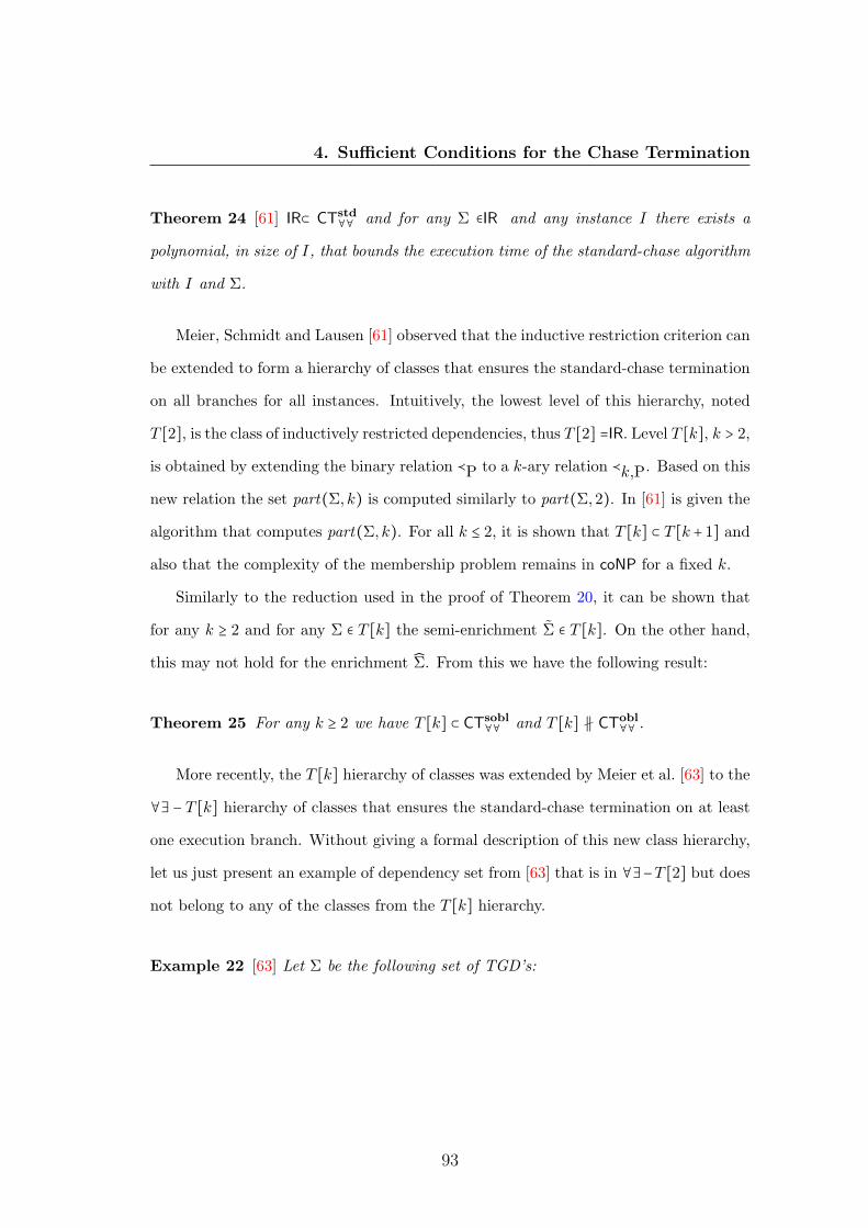
4. Sufficient Conditions for the Chase Termination
Theorem 24 [61] IR⊂ CTstd∀∀ and for any Σ ∈IR and any instance I there exists a
polynomial, in size of I, that bounds the execution time of the standard-chase algorithm
with I and Σ.
Meier, Schmidt and Lausen [61] observed that the inductive restriction criterion can
be extended to form a hierarchy of classes that ensures the standard-chase termination
on all branches for all instances. Intuitively, the lowest level of this hierarchy, noted
T [2], is the class of inductively restricted dependencies, thus T [2] =IR. Level T [k], k > 2,
is obtained by extending the binary relation ≺P to a k-ary relation ≺k,P. Based on this
new relation the set part(Σ, k) is computed similarly to part(Σ,2). In [61] is given the
algorithm that computes part(Σ, k). For all k ≤ 2, it is shown that T [k] ⊂ T [k + 1] and
also that the complexity of the membership problem remains in coNP for a fixed k.
Similarly to the reduction used in the proof of Theorem 20, it can be shown that
for any k ≥ 2 and for any Σ ∈ T [k] the semi-enrichment Σ ∈ T [k]. On the other hand,
this may not hold for the enrichment Σ. From this we have the following result:
Theorem 25 For any k ≥ 2 we have T [k] ⊂ CTsobl∀∀ and T [k] ∦ CTobl
∀∀ .
More recently, the T [k] hierarchy of classes was extended by Meier et al. [63] to the
∀∃ − T [k] hierarchy of classes that ensures the standard-chase termination on at least
one execution branch. Without giving a formal description of this new class hierarchy,
let us just present an example of dependency set from [63] that is in ∀∃−T [2] but does
not belong to any of the classes from the T [k] hierarchy.
Example 22 [63] Let Σ be the following set of TGD’s:
93

4. Sufficient Conditions for the Chase Termination
ξ1 ∶ R(x) → S(x,x)
ξ2 ∶ S(x, y) → ∃z T (y, z)
ξ3 ∶ S(x, y) → T (x, y), T (y, x)
ξ4 ∶ T (x, y), T (x, z), T (z, x) → R(y)
ξ5 ∶ T (x, y) → E(x, y)
ξ6 ∶ U(x),E(x, y) → E(y, x)
ξ7 ∶ U(x),E(x, y) → ∃z E(y, z),E(z, x)
It is obvious that Σ ∈ CTstd∀∃ , as one may apply a terminating chase sequence on
Σ′ = {ξ1, ξ2, ξ3, ξ4} and then apply the rest of the rules from Σ. Note that, by applying
the rest of the rules, it will not affect the satisfiability of Σ′. Also note that both chase
sequences applied are terminating for all instances. Even more, in [63] it is shown that
Σ does not belong to any class from the T [k] hierarchy and that Σ ∈ ∀∃ − T [2].
4.9 Comparison between Classes
Before concluding this chapter dedicated to present different classes of dependencies
which ensure the termination of one or more chase algorithms, let us review how these
classes compare to each other and for which chase variation algorithm they ensure
termination.
From the practical point of view one of most important questions is regarding the
complexity of testing if a set of dependencies belongs to a given class. Figure 4.6
illustrates the complexity for the following problem: given C a class of dependency
sets and Σ a set of dependencies Is Σ ∈S?, note that for the classes with membership
problem in NP there was not yet proved a lower bound.
Next let us review for which algorithm these classes ensure termination given the
94

4. Sufficient Conditions for the Chase Termination
SW RA WA SD SwA Str CStr IR/T [k]Complexity P P P P P in NP in NP in NP
Figure 4.6: Set order between the presented classes
classes presented in this chapter. In Figure 4.7 we present each class of dependency sets
described in this section together with the termination criteria introduced in Chapter
3. The symbol “+“ mentiones that the given class is sufficient for the chase algorithm
termination with the given criterion. Note also that there are not mentioned all the
termination criteria because of the following equalities: CTobl∀∀ = CTobl
∀∃ , CTsobl∀∀ = CTsobl
∀∃ ,
CTres∀∀ = CTres
∀∃ and CTcore∀∀ = CTcore
∀∃ .
CTobl∀∀ CTsobl
∀∀ CTstd∀∀ CTres
∀∀ CTstd∀∃ CTcore
∀∀
SW + + + + + +RA + + + + + +WA + + + + +SD + + + + +SwA + + + + +Str + +CStr + + + + +IR/T [k] + + + + +
Figure 4.7: Classes ensuring termination for different chase algorithms
For an easier view we represent the set based comparison between different classes of
dependency as a Hasse diagram in Figure 4.8. Before concluding this section we need to
mention that more recently Greco et al. [41] extended the classes of dependencies that
ensure the standard-chase termination to new larger classes based on the stratification
method.
95

4. Sufficient Conditions for the Chase Termination
Figure 4.8: Hasse diagram corresponding to classes of dependency sets
96

4. Sufficient Conditions for the Chase Termination
4.10 The Rewriting Approach
Spezzano and Greco [70] noticed that all the previous classes may be properly extended
using a rewriting technique similarly to the Magic Sets rewriting method [12]. Intu-
itively, if T is one of the classes WA, SD, SwA, Str and CStr, then instead of directly
checking if a set of dependencies Σ ∈ T, we check if Adn(Σ) ∈ T, where Adn(Σ) is an
adornment based rewriting of Σ such that, for any instance I, the universal solutions
under Σ and I are the ”same” (with some schema transformations) with the set of
universal solutions under Adn(Σ) and I. Where the adornment of a predicate p of
arity m is a string of length m over the alphabet {b, f }. An adorned atom is of the
form pα1,α2,...,αm(x1, x2, . . . , xm); if αi = b, then the variable xi is considered bounded,
otherwise the variable is considered free.
We will present this method by using an example from [70]. Consider the following
set of dependencies Σ = {ξ1, ξ2}:
ξ1 ∶ N(x) → ∃y E(x, y)
ξ2 ∶ S(x),E(x, y) → N(y)
The affected positions in Σ are (E,1),(E,2) and (N,1). Because the propaga-
tion graph corresponding to Σ contains a cycle through an existential edge involving
positions (N,1) and (E,2), it follows that Σ ∉SD.
Let us now construct the set of dependencies Adn(Σ) as follows:
1. For all predicate symbols p of arity m in Σ add the TGD:
∀x1, x2, . . . , xm p(x1, x2, . . . , xm) → pα1,α2,...,αm(x1, x2, . . . , xm)
where, for all positive i ∈ [m], αi = b.
In our example Σ contains the following relational symbols {E,S,N}, that is we
97

4. Sufficient Conditions for the Chase Termination
add to Adn(Σ) the following set of TGD’s:
ξ′1 ∶ E(x, y) → Eb b(x, y)
ξ′2 ∶ N(x) → Nb(x)
ξ′3 ∶ S(x) → Sb(x)
2. Repeat to create new adornment predicate symbols based on the existing de-
pendencies, until none can be added. That is a variable in the head is marked
as bounded (free) and if it occurs only bounded (free) places in the body. All
existential variables in the head are marked as free.
Returning to the example, by using ξ1 from Σ and the new adornment Nb , we
add the following dependency to Adn(Σ)
ξ′4 ∶ Nb(x) → ∃y Eb f (x, y)
Similarly based on TGD ξ2 from Σ and new adornments Sb and Eb b , we add
the following dependency to Adn(Σ)
ξ′5 ∶ Sb(x),Eb b(x, y) → Nb(y)
Repeating this process, we add the following TGD’s to Adn(Σ):
ξ′6 ∶ Sb(x),Eb f (x, y) → N f (y)
ξ′7 ∶ N f (x) → ∃y Ef f (x, y)
After this point no other adornments can be created.
3. Finally, for each of the adornment predicate pα in Adn(Σ) add a new dependency
in Adn(Σ) that ”copies” pα to a new p predicate symbol. For the previous
98
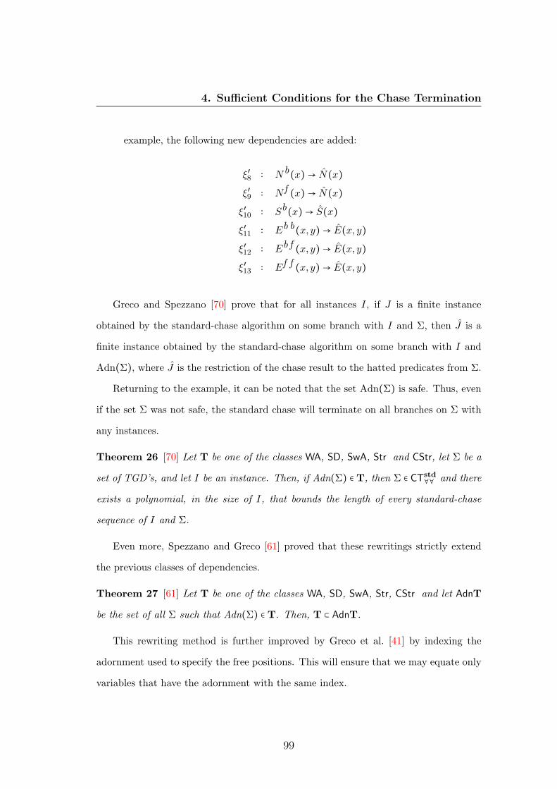
4. Sufficient Conditions for the Chase Termination
example, the following new dependencies are added:
ξ′8 ∶ Nb(x) → N(x)
ξ′9 ∶ N f (x) → N(x)
ξ′10 ∶ Sb(x) → S(x)
ξ′11 ∶ Eb b(x, y) → E(x, y)
ξ′12 ∶ Eb f (x, y) → E(x, y)
ξ′13 ∶ Ef f (x, y) → E(x, y)
Greco and Spezzano [70] prove that for all instances I, if J is a finite instance
obtained by the standard-chase algorithm on some branch with I and Σ, then J is a
finite instance obtained by the standard-chase algorithm on some branch with I and
Adn(Σ), where J is the restriction of the chase result to the hatted predicates from Σ.
Returning to the example, it can be noted that the set Adn(Σ) is safe. Thus, even
if the set Σ was not safe, the standard chase will terminate on all branches on Σ with
any instances.
Theorem 26 [70] Let T be one of the classes WA, SD, SwA, Str and CStr, let Σ be a
set of TGD’s, and let I be an instance. Then, if Adn(Σ) ∈ T, then Σ ∈ CTstd∀∀ and there
exists a polynomial, in the size of I, that bounds the length of every standard-chase
sequence of I and Σ.
Even more, Spezzano and Greco [61] proved that these rewritings strictly extend
the previous classes of dependencies.
Theorem 27 [61] Let T be one of the classes WA, SD, SwA, Str, CStr and let AdnT
be the set of all Σ such that Adn(Σ) ∈ T. Then, T ⊂ AdnT.
This rewriting method is further improved by Greco et al. [41] by indexing the
adornment used to specify the free positions. This will ensure that we may equate only
variables that have the adornment with the same index.
99

Chapter 5
Data Exchange, Repair and
Correspondence
In this chapter we will review three of the problems that make use of the chase procedure
in the process of finding “solutions“. First we will review the Data Exchange problem
and see what type of solutions are computed by the standard-chase algorithm, next we
will show how this result is improved by using the extended-core-chase algorithm. The
third section will review the Data Repair problems and present how the standard-chase
procedure helps in solving some of these problems in polynomial time for special classes
of dependencies. Finally we formally introduce the Data Correspondence setting and
check two of the main problems associated with this setting, that is solution-existence
and solution-check problems; and we will show how the standard-chase algorithm helps
to get tractability results for some cases. Part of the results of this section was first
published in [37].
100
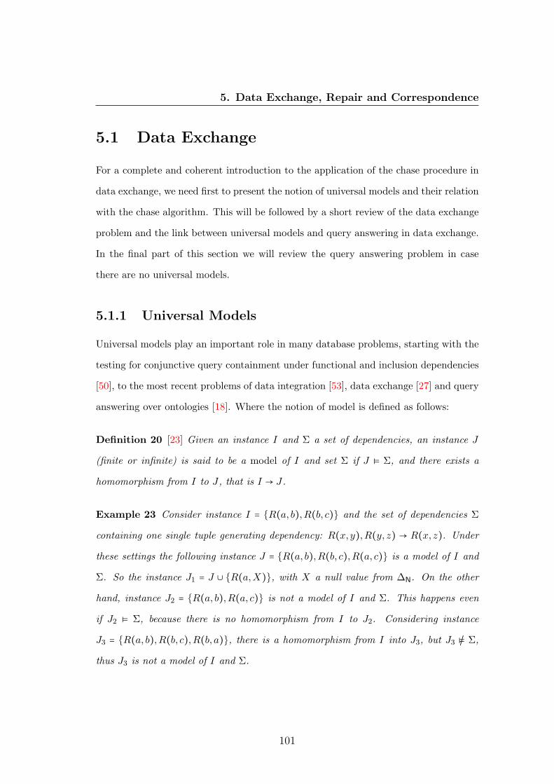
5. Data Exchange, Repair and Correspondence
5.1 Data Exchange
For a complete and coherent introduction to the application of the chase procedure in
data exchange, we need first to present the notion of universal models and their relation
with the chase algorithm. This will be followed by a short review of the data exchange
problem and the link between universal models and query answering in data exchange.
In the final part of this section we will review the query answering problem in case
there are no universal models.
5.1.1 Universal Models
Universal models play an important role in many database problems, starting with the
testing for conjunctive query containment under functional and inclusion dependencies
[50], to the most recent problems of data integration [53], data exchange [27] and query
answering over ontologies [18]. Where the notion of model is defined as follows:
Definition 20 [23] Given an instance I and Σ a set of dependencies, an instance J
(finite or infinite) is said to be a model of I and set Σ if J ⊧ Σ, and there exists a
homomorphism from I to J , that is I → J .
Example 23 Consider instance I = {R(a, b),R(b, c)} and the set of dependencies Σ
containing one single tuple generating dependency: R(x, y),R(y, z) → R(x, z). Under
these settings the following instance J = {R(a, b),R(b, c),R(a, c)} is a model of I and
Σ. So the instance J1 = J ∪ {R(a,X)}, with X a null value from ΔN. On the other
hand, instance J2 = {R(a, b),R(a, c)} is not a model of I and Σ. This happens even
if J2 ⊧ Σ, because there is no homomorphism from I to J2. Considering instance
J3 = {R(a, b),R(b, c),R(b, a)}, there is a homomorphism from I into J3, but J3 /⊧ Σ,
thus J3 is not a model of I and Σ.
101
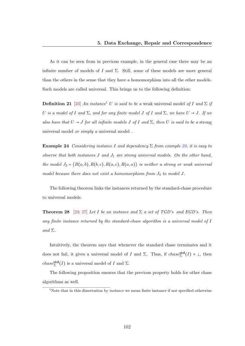
5. Data Exchange, Repair and Correspondence
As it can be seen from in previous example, in the general case there may be an
infinite number of models of I and Σ. Still, some of these models are more general
than the others in the sense that they have a homomorphism into all the other models.
Such models are called universal. This brings us to the following definition:
Definition 21 [23] An instance1 U is said to be a weak universal model of I and Σ if
U is a model of I and Σ, and for any finite model J of I and Σ, we have U → J . If we
also have that U → J for all infinite models J of I and Σ, then U is said to be a strong
universal model or simply a universal model .
Example 24 Considering instance I and dependency Σ from example 23, it is easy to
observe that both instances J and J1 are strong universal models. On the other hand,
the model J3 = {R(a, b),R(b, c),R(a, c),R(a, a)} is neither a strong or weak universal
model because there does not exist a homomorphism from J3 to model J .
The following theorem links the instances returned by the standard-chase procedure
to universal models.
Theorem 28 [23; 27] Let I be an instance and Σ a set of TGD’s and EGD’s. Then
any finite instance returned by the standard-chase algorithm is a universal model of I
and Σ.
Intuitively, the theorem says that whenever the standard chase terminates and it
does not fail, it gives a universal model of I and Σ. Thus, if chasestdΣ (I) ≠ %, then
chasestdΣ (I) is a universal model of I and Σ.
The following proposition ensures that the previous property holds for other chase
algorithms as well.
1Note that in this dissertation by instance we mean finite instance if not specified otherwise
102

5. Data Exchange, Repair and Correspondence
Proposition 16 If chase∗Σ(I) ≠ %, then chase∗Σ(I) is a universal model of I and Σ,
where ∗ is one of the following chase variations: oblivious, semi-oblivious, restricted
and core.
Proof: In Chapter 3 we showed that for oblivious, semi-oblivious and restricted-chase
variations represented here by ∗, if chase∗Σ(I) ≠ %, then chasestdΣ (I) ≠ %. Also, in
the same chapter it was shown that if chase∗Σ(I) ≠ %, then it is that chase∗Σ(I) ⊧ Σ
and chase∗Σ(I) ↔ chasestdΣ (I). This property also holds for the core chase as shown
in Theorem 29. The direct consequence is that chase∗Σ(I) is a universal model of I
and Σ∎
The previous result ensures that the chase procedure computes universal models of
its input. Naturally the following question raises: are these algorithms also complete in
finding universal models? The following example shows that we have a negative answer
to this question in case of the standard chase.
Example 25 Let us consider the same instance I = {R(a, b)} and Σ = {ξ1, ξ2} a set of
TGD’s as in Example 8:
ξ1 ∶ ∀x, y R(x, y) → ∃z R(y, z)
ξ2 ∶ ∀x, y R(x, y),R(y, z) → R(y, y)
As shown in Example 8, there is no terminating branch for the standard-chase
algorithm, but there exists universal model J = {R(a, b),R(b, b)} of I and Σ. Thus the
standard chase is not complete in finding universal models.
The result below shows that there exists one chase variation, namely the core chase,
that is complete in finding universal models.
103

5. Data Exchange, Repair and Correspondence
Theorem 29 [23] Let I be an instance and Σ a set of TGD’s and EGD’s. Then there
exists a universal model of I and Σ iff the core-chase algorithm terminates on input I
and Σ. Even more, chasecoreΣ (I) is a universal model of I and Σ.
From the definition of the universal models it follows that all universal models are
also weak universal models. The following example shows that the converse does not
always hold.
Example 26 [23] Let us consider instance I = {T (a)} and set Σ = {ξ1, ξ2, ξ3} of
TGD’s:
ξ1 ∶ T (x) → ∃y, z E(y, z)
ξ2 ∶ E(x, y) → ∃z E(y, z)
ξ3 ∶ E(x, y),E(y, z) → E(x, z)
Considering that relation E contains edges of a graph, clearly all models have an
infinite walk in the graph. This means that for every finite model it has a cycle in the
corresponding graph. From this and ξ3, it follows that any finite model has a self loop.
Then the instance J = {T (a),E(X,X)} is a model of I and Σ containing a self loop.
Consequently, J is a weak universal model of I and Σ. On the other hand, the transitive
closure of an infinite path also satisfies Σ, however no finite instance with cycle has a
homomorphism into it. This means that J is not a strong universal model of I and Σ.
We cannot conclude this section on universal models without emphasizing the result
of Deutsch et al. [23] showing that it is undecidable to say if an instance U is a strong
(weak) universal model of instance I and Σ a set of tgds. Even more, they demonstrated
that there is no complete chase based procedure for finding weak universal models.
104

5. Data Exchange, Repair and Correspondence
5.1.2 Solutions in Data Exchange
Data exchange is an old database problem that earned more formal treatment only
recently. More precisely, data exchange is the problem of transforming data structured
under a source schema to data structured under a different target schema. The concept
of mappings between schemata was introduced by Bernstein et al. in [14] and by Miller
et al. [65] for relational schemata. Let S and T be two disjoint schemata, which we
call the source schema and the target schema, respectively. A data exchange mapping
(or simply mapping) M from source S to target T is a set of pairs (I, J), where I is
an instance over schema S and I is an instance over schema T. Thus
M = {(I, J) ∣ I ∈ Inst(S) and J ∈ Inst(T)}. (5.1)
In most of the practical applications the data exchange mapping M is specified as
a tuple (S,T,Σst,Σt), where S represents the source schema, T represents the target
schema, Σst is a set of constraints representing the relationship between the source and
target schema, and Σt represents a set of constraints over the target schema. Thus, if
I ∈ Inst(S) and J ∈ Inst(T), then (I, J) ∈ M iff I ∪J ⊧ Σst ∪Σt. In this dissertation if
not mentioned otherwise, we will consider a mapping specified as previously.
Definition 22 Given a data exchange mapping M = (S,T,Σst,Σt) and instance I
over the source schema S, the data exchange problem is to find instances J , over the
target schema T, such that I ∪ J is a model for I and Σst ∪ Σt. An instance J with
the previous properties is called a solution to the data exchange problem, or simply a
solution.
Note that the solution to the data exchange problem is not necessarily a ground
instance. By SolM(I) is denoted the set of all ground data exchange problem solution
for a mapping M and source instance I.
105

5. Data Exchange, Repair and Correspondence
The data exchange problem was first formalized by Fagin et al. in their seminal
paper [27]. Most of the data exchange problems considered have Σst specified by a set of
TGD’s and Σt specified by a set of TGD’s and EGD’s. The mapping over this classes
of dependencies covers most of the practical mappings. From now on, if not mentioned
otherwise, we assume that the data exchange dependencies are of this format.
As there may be an infinite number of solutions to a given data exchange problem, a
natural question raises: which solution, or finite set of solutions, should be materialized
on the target? Unfortunately, there is no simple answer to this question, because it
also depends on the use of the solutions. In this subsection, we consider one of the
common cases when solutions are used to get certain answers for a set of union of
conjunctive queries (UCQ) over the target instance. This can be formalized by the
following definition:
Definition 23 Let M = (S,T,Σst,Σt), also let I be a source instance and q a query
in UCQ over schema T. The certain answer of q for I under M is defined as
certainM(q, I) =def ⋂J∈SolM (I)
Q(J)
Fagin et al. [27] showed that the universal solution is a good candidate for materi-
alization in data exchange problem under the certain UCQ answer semantics. For more
clarity, an instance J is a universal solution for source instance I and data exchange
setting M = (S,T,Σst,Σt) if J is a solution for I and M and for all solutions K for
I and M we have J → K. It can be noted that a strong correlation exists between
the notion of data exchange solution and that of model, and correspondingly between
the notion of universal solution and universal model. Thus, any solution for a data
exchange mapping M = (S,T,Σst,Σt) and instance I is the restriction over the target
schema T for a model of I and the dependencies Σst ∪ Σt. Similarly, any universal
solution for M and I is also a universal model of I and the dependencies of Σst ∪ Σt
106

5. Data Exchange, Repair and Correspondence
restricted to the target schema. This means that all results specified in subsection 5.1.1
also hold for universal solutions. In particular, it means that the universal solution can
be computed by the standard-chase algorithm and it is undecidable if the universal
solution exists for a given mapping M and a given instance I. The following propo-
sition extends this result by showing that it is undecidable for a given mapping if the
standard chase will terminate for all source instances.
Proposition 17 Given a mapping M , it is undecidable if the standard (oblivious/semi-
oblivious/restricted/core) chase terminates for all source instances.
Proof: We will reduce the problem of deciding if the standard (oblivious/semi-oblivious
/restricted/core) chase terminates for an instance I and set of dependencies Σ to the
stated problem. For this, let us consider an instance I and set of dependencies Σ both
over schema R. Construct TGD ξ from I as follows:
ξ ∶ → R1(a1),R2(a2), . . . ,Rn(an)
such that head(ξ) = I. Consider Σt = Σ∪{ξ}, Σst = ∅ and mapping M = (∅,R,Σst,Σt).
We can observe that the standard chase for mapping M and any instance I ′ terminates
if and only if the standard chase terminates on input I and Σ. From this reduction and
Theorem 2 (and correspondingly Theorems 3, 7, 8, 11) it follows that it is undecidable if
the standard (oblivious/semi-oblivious/restricted/core) chase terminates for all source
instances for a given mapping M∎
In [27], Fagin et al. present a sufficient condition for the universal solution to not
exist, as shown in the following theorem:
Theorem 30 [27] Let M = (S,T,Σst,Σt) be a mapping and I be a source instance
such that there is a failing branch for the standard chase with input I and Σst ∪ Σt.
Then there is no universal solution for I and M .
107

5. Data Exchange, Repair and Correspondence
In data exchange we may also have settings for which there exist solutions, but
there is no universal solution.
Example 27 Consider the mapping specified as follows:
M = ({S},{R},{S(x, y) → R(x, y)},{R(x, y) → ∃z R(y, z)})
and the source instance I = {S(a, b)}. Clearly, because of the second dependency, there
is no universal solution for this setting, but there exists a solution J = {R(a, b),R(b, b)}.
Kolaitis et al. in [52] proved that it is undecidable to check for a given instance I
and a mapping M if there exists a solution for I and M .
Before presenting how to compute the certain answers on target schema for UCQ
queries in a data exchange mapping using a universal solution, let us introduce the
notion of naıve evaluation as presented in [55]. Let I be an instance, possible with
null values, and q be a UCQ query. The qnaıve(I) is defined by evaluating q on I by
treating each null as new special constant, and then by eliminating from the result all
the tuples that contain such special constants.
Theorem 31 [27] Let M = (S,T,Σst,Σt) be a mapping and I an instance over the
source schema that does not contain nulls. Suppose also that there exists a universal
solution J for I and M . Then, certainM(q, I) = qnaıve(J) for any q ∈UCQ.
Libkin [55] showed that UCQ is the largest class of queries with the property that
the certain answers may be computed using the naıve evaluation. We may note here
the result from [27] which states that for a data exchange mapping M specified by a
weakly acyclic set of TGD’s one may get the certain answers to a union of conjunctive
query with at most one unequality per disjunct over an instance I and M from the
universal solution in polynomial time in the size of the data. This does not contradict
108

5. Data Exchange, Repair and Correspondence
with Libkin’s result as the certain answer to the query is not computed using the naıve
evaluation. We conclude this subsection by reiterating the result which specifies that
between the infinite set of universal solution there exists a universal solution which is
minimal in size. Such universal solution is called the core solution and, as noted in
[28], it is unique up to variable renaming. Even more, in [23] it was proved that if
there exists a universal solution then its core can be computed using the core-chase
algorithm.
5.1.3 Data Exchange beyond Universal Solutions
It is known that there is no universal solution for the mapping and the source instance
from Example 27. On the other hand, when considering the query q(x) ← ∃y R(x, y),
the certain answer contains the tuples {(a), (b)} . In their seminal paper [16], Cali,
Gottlob and Kifer investigate the problem of conjunctive query answering when the
universal solution is not guaranteed to exist. For this, the authors unravel two classes
of TGD’s , namely guarded tuple generating dependencies (GTGD) and weakly guarded
tuple generating dependencies (WGTGD), for which the problem of conjunctive query
evaluation is decidable. Intuitively, a TGD is guarded if its body contains an atom
called guard that covers all the variables in the body. Clearly LAV dependencies are
GTGD’s. A set of TGD’s is said to be weakly guarded if for each TGD its body
contains one atom that covers all the variables that appear in the affected position.
That is predicate positions that may contain new labeled nulls generated during the
chase process.
Example 28 Let us consider the following dependencies:
ξ1 ∶ S(x),R(x, y) → ∃z R(y, z)
ξ2 ∶ R(x, z),R(z, y) → R(y, x)
109

5. Data Exchange, Repair and Correspondence
In ξ1, the atom R(x, y) covers all the variables in the body, meaning that it is a
GTGD. Clearly, ξ2 is not GTGD as there is no atom to cover all variables from the
body. The affected position for the set {ξ1, ξ2} is (R,2), meaning that we may introduce
new labeled nulls during the chase process only in the second position of R. Because in
ξ2 the atom R(z, y) covers both variables that appear in the affected position in ξ2, it
follows that ξ2 is a WGTGD.
Cali et al. [16] give data complexity bounds for the conjunctive query answering
problem. This problem is expressed as follows: Does a tuple t belong to the certain
answer for a mapping M and a source instance I? In their paper, the complexity
bounds discovered are: (1) for a fixed set GTGD’s , the conjunctive query answering
problem is NP-complete; (2) for atomic queries, the problem becomes polynomial; (3) in
case the fixed dependencies are WGTGD’s , the conjunctive query answering problem
becomes EXPTIME-complete. More recently other classes of dependencies for which
one may get the certain answers to conjunctive queries are revealed by Cali et al. in
[19].
A universal solution is enough to compute certain answer for any UCQ query under
the certain answer semantics for UCQ queries over the target schema. Therefore, the
following question rises: Is this semantics also a good model for general queries? As
shown in [7] and [54], this semantics is not suitable for general queries, as it may give
unintuitive answers even for simple copying data exchange settings.
Example 29 Let us consider a data exchange setting M = ({R},{R′},Σst,∅), where
Σst simply copies the source into target: R(x, y) → R′(x, y). Consider the source
instance I = {R(a, b)} and query over the target schema q(x, y) ← R′(x, y) ∧¬R′(x,x).
Since one of the solution is instance J = {R′(a, b),R′(a, a)}, it follows that the certain
answer certainM(q, I) = ∅. Now, when applying the same query on the source instance
(by replacing relation name R′ with R), it returns the set of tuples {(a, b)}. Clearly
110

5. Data Exchange, Repair and Correspondence
this is not the expected behavior as the target instance is supposed to be a copy of the
source instance.
In order to solve the problems related to general queries, new closed world seman-
tics were proposed for the data exchange problem [38; 44; 45; 47; 54]. Libkin [54]
replaced universal solutions with a set of CWA-solutions (that are in fact universal
solutions), used afterwards to compute certain answers for FO queries. Hernich and
Schweikardt [47] introduced a new chase based algorithm, called the α-chase, to com-
pute CWA-presolutions, these are instances useful to compute the set of CWA-solutions.
In Chapter 6 we introduce a new closed world semantics and we argue that it is suitable
for the data exchange problem. The representation of the solution set in this case will
be done using conditional tables. A similar chase process for conditional tables that
consider only source-to-target dependencies was recently introduced in [10].
We close this sub-chapter by also mentioning the work of Afrati, Li and Pavlaki [5]
that extended the data exchange problem by considering dependencies with arithmetic
comparisons.
5.2 Data Repair
Data repair (or database repair) is one of the main problems associated with incon-
sistent databases. A data repair solution for an inconsistent database instance is a
consistent database instance over the same schema that differs minimally from the
initial instance. Based on the minimality criterion, different approaches are used:
symmetric-difference repair presented by Arenas et al. in [8]; subset-repairs as devel-
oped by Chomicki and Marcinkowski in [22]; cardinality repair proposed by Lopatenko
and Bertosi in [57]; attribute based repairs proposed by Wijsen [75] and the newly in-
troduced component-cardinality repair by Afrati and Kolaitis in [4]. The most studied
111
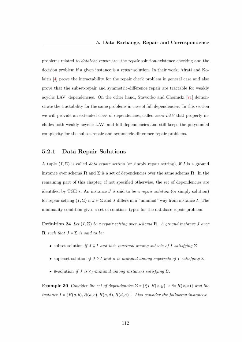
5. Data Exchange, Repair and Correspondence
problems related to database repair are: the repair solution-existence checking and the
decision problem if a given instance is a repair solution. In their work, Afrati and Ko-
laitis [4] prove the intractability for the repair check problem in general case and also
prove that the subset-repair and symmetric-difference repair are tractable for weakly
acyclic LAV dependencies. On the other hand, Staworko and Chomicki [71] demon-
strate the tractability for the same problems in case of full dependencies. In this section
we will provide an extended class of dependencies, called semi-LAV that properly in-
cludes both weakly acyclic LAV and full dependencies and still keeps the polynomial
complexity for the subset-repair and symmetric-difference repair problems.
5.2.1 Data Repair Solutions
A tuple (I,Σ) is called data repair setting (or simply repair setting), if I is a ground
instance over schema R and Σ is a set of dependencies over the same schema R. In the
remaining part of this chapter, if not specified otherwise, the set of dependencies are
identified by TGD’s. An instance J is said to be a repair solution (or simply solution)
for repair setting (I,Σ) if J ⊧ Σ and J differs in a “minimal“ way from instance I. The
minimality condition gives a set of solutions types for the database repair problem.
Definition 24 Let (I,Σ) be a repair setting over schema R. A ground instance J over
R such that J ⊧ Σ is said to be:
• subset-solution if J ⊆ I and it is maximal among subsets of I satisfying Σ.
• superset-solution if J ⊇ I and it is minimal among supersets of I satisfying Σ.
• ⊕-solution if J is ≤I-minimal among instances satisfying Σ.
Example 30 Consider the set of dependencies Σ = {ξ ∶ R(x, y) → ∃z R(x, z)} and the
instance I = {R(a, b),R(a, c),R(a, d),R(d, a)}. Also consider the following instances:
112
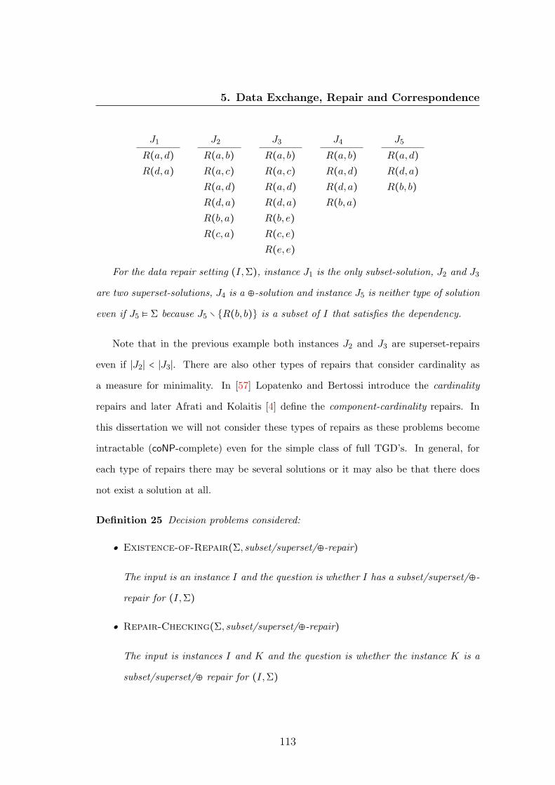
5. Data Exchange, Repair and Correspondence
J1
R(a, d)R(d, a)
J2
R(a, b)R(a, c)R(a, d)R(d, a)R(b, a)R(c, a)
J3
R(a, b)R(a, c)R(a, d)R(d, a)R(b, e)R(c, e)R(e, e)
J4
R(a, b)R(a, d)R(d, a)R(b, a)
J5
R(a, d)R(d, a)R(b, b)
For the data repair setting (I,Σ), instance J1 is the only subset-solution, J2 and J3
are two superset-solutions, J4 is a ⊕-solution and instance J5 is neither type of solution
even if J5 ⊧ Σ because J5 ∖ {R(b, b)} is a subset of I that satisfies the dependency.
Note that in the previous example both instances J2 and J3 are superset-repairs
even if ∣J2∣ < ∣J3∣. There are also other types of repairs that consider cardinality as
a measure for minimality. In [57] Lopatenko and Bertossi introduce the cardinality
repairs and later Afrati and Kolaitis [4] define the component-cardinality repairs. In
this dissertation we will not consider these types of repairs as these problems become
intractable (coNP-complete) even for the simple class of full TGD’s. In general, for
each type of repairs there may be several solutions or it may also be that there does
not exist a solution at all.
Definition 25 Decision problems considered:
• Existence-of-Repair(Σ, subset/superset/⊕-repair)
The input is an instance I and the question is whether I has a subset/superset/⊕-
repair for (I,Σ)
• Repair-Checking(Σ, subset/superset/⊕-repair)
The input is instances I and K and the question is whether the instance K is a
subset/superset/⊕ repair for (I,Σ)
113
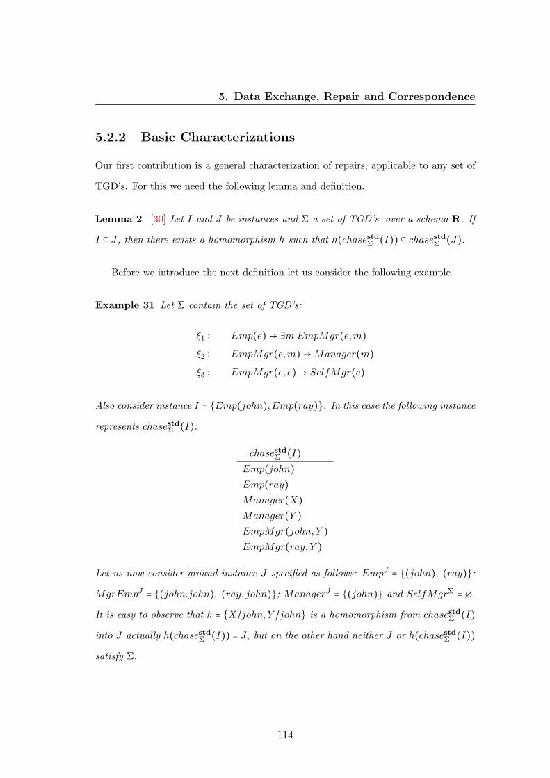
5. Data Exchange, Repair and Correspondence
5.2.2 Basic Characterizations
Our first contribution is a general characterization of repairs, applicable to any set of
TGD’s. For this we need the following lemma and definition.
Lemma 2 [30] Let I and J be instances and Σ a set of TGD’s over a schema R. If
I ⊆ J , then there exists a homomorphism h such that h(chasestdΣ (I)) ⊆ chasestd
Σ (J).
Before we introduce the next definition let us consider the following example.
Example 31 Let Σ contain the set of TGD’s:
ξ1 ∶ Emp(e) → ∃m EmpMgr(e,m)
ξ2 ∶ EmpMgr(e,m) → Manager(m)
ξ3 ∶ EmpMgr(e, e) → SelfMgr(e)
Also consider instance I = {Emp(john),Emp(ray)}. In this case the following instance
represents chasestdΣ (I):
chasestdΣ (I)
Emp(john)Emp(ray)Manager(X)Manager(Y )EmpMgr(john,Y )EmpMgr(ray, Y )
Let us now consider ground instance J specified as follows: EmpJ = {(john), (ray)};
MgrEmpJ = {(john.john), (ray, john)}; ManagerJ = {(john)} and SelfMgrΣ = ∅.
It is easy to observe that h = {X/john,Y /john} is a homomorphism from chasestdΣ (I)
into J actually h(chasestdΣ (I)) = J , but on the other hand neither J or h(chasestd
Σ (I))
satisfy Σ.
114

5. Data Exchange, Repair and Correspondence
The previous example leads to the introduction of a new type of homomorphism
called Σ-satisfying homomorphism:
Definition 26 Given an instance K and a set Σ of TGD’s over a schema R, as
well as a ground instance I over R, a Σ-satisfying homomorphism from K into I is a
homomorphism h from K into I, such that h(K) ⊆ J ⊆ I, and J ⊧ Σ, for some J ⊆ I.
We can now state some necessary and sufficient conditions for which an instance
K, such that K ⊧ Σ, is a ⊕-repair for a given repair setting (I,Σ). The first condition
of this theorem assures that K ∖ I does not contain superfluous tuples. The second
condition guarantees that no more tuples from I could be added to K and still satisfy
the dependencies.
Theorem 32 Let Σ be a set of TGD’s, I and K two ground instances such that K ⊧ Σ.
Then K is a ⊕-repair for (I,Σ) if and only if the following conditions are satisfied:
1. For all Σ-satisfying homomorphisms h such that h(chasestdΣ (I ∩K)) ⊆ K, and
all instances J ⊆ K, such that J ⊧ Σ and h(chasestdΣ (I ∩K)) ⊆ J , it holds that
J = K.
2. There do not exist a tuple t ∈ I ∖K and Σ-satisfying homomorphism h with an
instance J ⊆ K ∪ I, J ⊧ Σ, such that h(chasestdΣ ((I ∩K) ∪ {t})) ⊆ J ⊆ K ∪ I.
Proof: Suppose K is a ⊕-repair for (I,Σ). As K ⊧ Σ, we have chasestdΣ (K) = K. From
Lemma 2 it is that there exists h with h(chasestdΣ (I ∩K)) ⊆ K. Toward a contradiction,
suppose that there exists a ground instance J , such that h(chasestdΣ (I ∩K)) ⊆ J ⊂ K
and J ⊧ Σ. Then J ∖ I ⊂ K ∖ I and, since I ∩K ⊆ chasestdΣ (I ∩K) and I ∩K is ground,
we have that I ∩K ⊆ J , meaning that I ∖ J ⊆ I ∖K, and consequently that J ≤I K.
But this contradicts the assumption that K is a ⊕-repair. Therefore it must be that
J = K, meaning that K satisfies condition 1.
115
5. Data Exchange, Repair and Correspondence
Suppose then that condition 2 is violated, and tuple t, Σ-satisfying homomorphism
h and instance J exist. Since, for such a J , we would have I ∖J ⊂ I ∖K, it would follow
that J ≤I K, contradicting the assumption that K is a ⊕-repair.
For the only if direction, let K be an instance such that K ⊧ Σ and K satisfies
conditions 1 and 2. We need to show that K is ≤I -minimal. If this is not the case,
there must be an instance J , such that J ⊧ Σ and J <I K. Thus J ∖ I ⊆ K ∖ I,
and I ∖ J ⊆ I ∖ K, and at least one of the inclusions is proper. Suppose first that
it were the case that I ∖ J = I ∖ K. Then we would have J ⊆ K. Thus, if J ∖ I
were to be a proper subset of K ∖ I, it would necessarily be that J ⊂ K. Since then
I ∩ K = I ∩ J , we have chasestdΣ (I ∩K) = chasestd
Σ (I ∩ J). By Lemma 2 we have a
homomorphism h, such that h(chasestdΣ (I ∩ J)) ⊆ chasestd
Σ (J) = J . Then it would hold
that h(chasestdΣ (I ∩K)) ⊆ J ⊂ K, contradicting condition 1.
If it were the case that I ∖ J ⊂ I ∖K, we would find a tuple t ∈ (J ∩ I) ∖ (K ∩ I),
that is in I ∖K, such that by Lemma 2 we would have a homomorphism h, such that
h(chasestdΣ ((I ∩K) ∪ {t})) ⊆ J ⊆ K ∪ I, a contradiction to the assumption that K
satisfies condition 2∎
5.2.3 Complexity Results
In order to introduce the data complexity results for the problems formalized in Defi-
nition 25, we need first to define some preliminary notions.
Definition 27 The Gaifman graph GI for an instance I is an undirected graph with
vertex set dom(I) and an edge between two vertices x and y if x and y appear together
in a tuple of I.
Definition 28 The Gaifman graph of nulls GIΔN
is the Gaifman graph GI restricted
to the nulls occurring in I.
116

5. Data Exchange, Repair and Correspondence
Definition 29 A block is a connected set of nulls in GIΔN
. Let N ⊆ ΔN. We denote
by blocks(N, I) the set of all blocks from the Gaifman graph of nulls GIΔN
restricted to
the nulls in N . If b is a block we denote by blocksize(b) the cardinality of b.
The blocksize definition is extended to an instance I. Thus blocksize(I) is the size
of the largest block of nulls in I. For an instance I, we said that it had a bounded block
size if there existed a constant c such that blocksize(I) ≤ c. In this case we say that
the blocksize is bounded by c. Clearly any finite instance has a bounded blocksize.
The next theorem is due to Fagin, Kolaitis and Popa [28] and was further highlighted
by Gottlob and Nash [34]. Note that any set of source-to-target tgds is non-recursive,
hence weakly acyclic.
Theorem 33 [28]
1. Let I be a ground instance, and Σ a weakly acyclic set of TGD’s. Then the size
of chasestdΣ (I) is polynomial in I.
2. Let I1 be a ground instance over R1 and I2 be a ground instance over R2. Let Σ
be a set of source-to-target TGD’s. Then chasestdΣ12
(I1 ∪ I2) has bounded blocksize.
3. Let I and K be instances such that blocksize(K) ≤ c, for some constant c. Then it
can be tested whether there exists a homomorphism from K to I in time O(∣K ∣c).
We will also use the following result obtained by Afrati and Kolaitis.
Theorem 34 [4] Let Σ be a set of weakly acyclic TGD’s and I an instance, such that
I ⊧ Σ. Then there exists a constant c, depending only on Σ, such that for each tuple
t ∈ I there is an instance Kt ⊆ I, such that t ∈ Kt,Kt ⊧ Σ, and ∣Kt∣ ≤ c.
Armed with these results we will derive a polynomial time algorithm that determines
the existence of database repair solution for weakly acyclic set of TGD’s.
117

5. Data Exchange, Repair and Correspondence
Theorem 35 Let Σ be a weakly acyclic set of TGD’s. Then the problem
Existence-of-Repair(Σ, subset)
can be solved in polynomial time.
Proof: Let (I,Σ) be a repair setting and c the constant mentioned in Theorem 34
Consider the following algorithm:
Repair-Search(I,Σ, c)
1 for i ← 1 to c
2 do for K ⊆ I, ∣K ∣ = i
3 do if K ⊧ Σ return true
4 return False
The algorithm is obviously sound. The completeness follows directly from Theo-
rem 34. The inner loop on line 2 is executed at most (∣I ∣i ) times and the outer loop on
line 1 at most c times. Thus, line 3 is executed at most ∣I ∣c times. Each execution of
line 3 is done in space logarithmic in at most c. Consequently, the algorithm runs in
time polynomial in the size of I∎
We note that Existence-of-Repair(Σ, superset) is a non-problem, since superset-
solutions always exist (recall that no egd’s are present). We now turn our attention to
the solution checking problem.
Afrati and Kolaitis derived the following complexity theoretic characterization for
repair checking with weakly acyclic TGD’s.
Theorem 36 [4] There is a weakly acyclic set Σ of TGD’s such that the following
problems: Repair-Checking(Σ, subset), Repair-Checking(Σ,⊕) are both coNP-
complete.
To this we can now add the missing piece.
118

5. Data Exchange, Repair and Correspondence
Theorem 37 There is a weakly acyclic set Σ of TGD’s such that the problem of
Repair-Checking(Σ, superset) is coNP-complete.
Proof: We will show that the complementary problem of deciding whether an instance
K is not a superset-repair of I w.r.t. Σ is NP-complete.
For the upper bound, we check in logarithmic space if K ⊧ Σ, if not, K is not
a superset-repair. Otherwise non-deterministically choose an instance J such that
K ⊃ J ⊇ I. It follows that K is not a superset-repair if and only if J ⊧ Σ. Again
the satisfaction can be tested in logarithmic space.
For the lower bound we will again reduce the Positive 1-In-3-SAT problem to
the superset-repair checking problem.
Recall the Positive 1-In-3-SAT is the following decision problem: given a Boolean
formula ϕ in a conjunctive normal form with each conjunct is a disjunction of exactly 3
literals, is there a truth assignment for ϕ that makes true exactly one variable in each
conjunct? This problem was showed by Schaefer [69] to be NP-complete.
Returning to our reduction, consider the schema having five relations P,T,S,D,E
of arities 3,2,3,2 and 1 respectively. The dependencies Σ will be :
P (x, y, z) → ∃u, v,w T (x,u), T (y, v), T (z,w), S(u, v,w)
T (x,u), T (x,u′),D(u,u′) → ∃y E(y)
T (x,u),E(y) → ∃u′ T (x,u′),D(u,u′)
Given an instance P of the Positive 1-In-3-SAT problem we construct I as
P I = {(x, y, z) ∶ x ∨ y ∨ z is a clause in P}
T I = ∅
SI = {(0,0,1), (0,1,0), (1,0,0)}
EI = ∅
DI = {(0,1), (1,0)}
and instance K as containing I plus the following tuples:
119

5. Data Exchange, Repair and Correspondence
TK = {(x,1), (x,0) ∶ x is a variable in P}
EK = {(0)}
This reduction clearly is being polynomial and, since obviously K ⊧ Σ, it remains only
to prove that there exists a truth assignment for P making exactly one variable in each
clause true if and only if K is not a superset-repair. For the if part suppose that there
exists such a truth assignment. Let J be an instance that contains I plus:
T J = {(x,u) ∶ u is the assignment for variable x in the solution of P}
It is easy to see that J ⊧ Σ and that K ⊃ J ⊇ I. In other words, K is not a
superset-repair.
For the only if part, suppose that K is not a superset-repair. This means that
there exists an instance J such that K ⊃ J ⊇ I, and J ⊧ Σ. As the inclusion between
J and K is proper, it means that there exists at least one tuple in K ∖ J . From the
construction of K it follows that the tuple is either in TK or in EK . If the tuple is in
TK , since J ⊧ Σ, the last dependency tells us that the tuple (0) cannot be in EJ . Then
the second dependency implies that T J contains a proper truth assignment, and the
first dependency implies that this truth assignment actually is Positive 1-In-3 and
satisfies P∎
In order to overcome the intractability barriers for the previous problems, it is clear
that the set Σ of dependencies has to be restricted. We next introduce a large class
of TGD’s for which all of the considered problems can be solved in polynomial time.
The proofs rely on recently developed homomorphism techniques (i.e. [4; 27; 33]), and
on the Σ-satisfying homomorphisms introduced in Definition 26.
First, we introduce the new class of TGD’s. For this, we need the concept of the
rank of a node in the dependency graph (see Definition 6) of a set Σ of TGD’s.
120

5. Data Exchange, Repair and Correspondence
Definition 30 ([27]) Let (R, i) be a vertex in the dependency graph of a set Σ of
TGD’s. Then rank(R, i) is the maximum number of existential edges along any path
in the graph ending in (R, i).
Lemma 3 ([27]) If Σ is a weakly acyclic set of TGD’s, then for each vertex (R, i)
of the dependency graph of Σ, rank(R, i) is finite and is bounded by some constant c
depending only on Σ.
Definition 31 Let Σ be a set of TGD’s over a schema R. For all relational symbols
R ∈ R that occur in Σ, we say that a position (R, i) is unsafe if rank(R, i) > 0. Any
relational symbol R that contains an unsafe position is said to be unsafe. A set Σ of
weakly acyclic dependencies is said to be semi-LAV if all unsafe relational symbols occur
in the body of LAV-dependencies only.
Example 32 Consider the following simple set of dependencies that is neither full or
LAV:
ξ1 ∶ R(x, y) → ∃z R(x, z), S(x)
ξ2 ∶ S(x), S(y) → ∃z R(x, z),R(z, y)
In this set we have rank(R,1) = 1, rank(R,2) = 2 and rank(S,1) = 0. Thus,
relation R is unsafe. On the other hand, relation R is safe so it may appear in the body
of the non-LAV dependency ξ2.
The class of semi-LAV TGD’s possesses several useful properties, as it will be shown
next.
Lemma 4 Let Σ be a set of semi-LAV TGD’s, let I be a ground instance and K be
the result of an arbitrary standard-chase sequence using Σ starting from I. Then for
any null X that occurs in K, the number of tuples in K containing X is bounded by a
constant that depends only on Σ.
121

5. Data Exchange, Repair and Correspondence
Proof: Let J be the first instance in the chase sequence from I to K where the null
X appears, and denote with JX the subset of tuples of J where X appears. If r is the
maximum number of atoms in the consequent of any dependency in Σ, it is clear that
∣JX ∣ ≤ r. Furthermore, as null value X can appear only in tuples of unsafe relations
(called unsafe tuples), it means that the tuples in JX can only be matched with the body
of some LAV-dependencies, each such body consisting of a single atom. Consequently,
the set of tuples KX in K that contain X can be generated by chasing JX using only
the LAV-dependencies in Σ. As Σ is weakly acyclic, it follows from Theorem 33 that
there is a polynomial p such that ∣KX ≤ p(∣JX ∣). Thus ∣KX ∣ ≤ p(r), which is a constant
depending only on Σ∎
Lemma 5 Let Σ be a set of weakly acyclic TGD’s, I a ground instance, and K the
result of some arbitrary standard -chase sequence using Σ starting from I. Then there
exists a partitioning {V0, V1, . . . , Vm} of the nulls in K, such that null X ∈ Vi iff X was
generated during the chase process using only nulls from {V0, . . . , Vi−1}.
Proof: Let N0,N1, . . . ,Nm be a partition of the nodes in the dependency graph of Σ
based on their rank. Since Σ is weakly acyclic, such a partitioning exists and, for any
dependency in Σ, the rank of the positions in the consequent is larger than or equal to
the rank of any position in the body of the dependency [27]. We show the existence
of the null partitioning constructively based on the chase steps. Initially let Vi be the
empty set for all i ∈ {0,1, . . . ,m}. During the chase process, when a new null X is
created in a position (R, i), we add this null to set V1, if there were no nulls in the
tuples that triggered the dependency. We add the null X to the set Vi if the set of nulls
belonging to the tuples that triggered the dependency that generated X is a subset of
{V0∪V1∪. . .∪Vi−1} and if there exists a null Y in that set such that Y ∈ Vi−1. Because the
rank of each position is at most m, it means that null X cannot be generated by a null
122
5. Data Exchange, Repair and Correspondence
belonging to Vm or higher. This proves the existence of partitioning {V0, V1, . . . , Vm}
of the nulls. Note that V0 = ∅∎
Theorem 38 Let Σ be a set of semi-LAV TGD’s, let I be a ground instance, and K
be the result of some arbitrary standard-chase sequence using Σ starting from I. Then
there is a constant c, depending only on Σ, such that blocksize(GK) ≤ c.
Proof: Recall that we denote by GK the Gaifman graph of nulls for instance K (see
Definition 28). Let {V0, V1, . . . , Vm} be the partitioning of the variables in K, as de-
scribed in Lemma 5. We prove by an induction on i that there are constants ci, such
that, for any block b ∈ blocks(V0 ∪⋯∪Vi,GK), we have blocksize(b) ≤ ci, meaning that
blocksize(GK) = max{blocksize(b) ∶ b ∈ blocks(V0 ∪⋯∪ Vm,GK)} ≤ cm.
Basis: Clearly V0 = ∅, and blocks(V0,GK) = ∅. We can therefore set c0 = 0.
Inductive step: Let b be a block in blocks(V0 ∪⋯∪ Vi,GK). If all the nulls in b are
in V0 ∪⋯ ∪ Vi−1, the block b is also in blocks(V0 ∪⋯ ∪ Vi−1,GK) and, by the inductive
hypothesis, we have blocksize(b) ≤ ci−1. Suppose then that X is a null in b from Vi.
This means that X was generated from variables in V0 ∪ ⋯ ∪ Vi−1 by an existential
dependency ξ. There are three cases to consider:
Case 1: ξ is a dependency with possibly several atoms in the body. Then all these
atoms are over safe relations, thus not mapped to nulls during the chase process. Thus
X, along with the other existential nulls in the consequent of ξ will form their own
block in blocks(V0 ∪ ⋯ ∪ Vi,GK), with blocksize at most s, where s is the maximum
number of special edges incident from any node in the dependency graph of Σ.
Case 2: ξ has a single unsafe atom in the body, but none of the (universally quan-
tified) variables in the body occurs in the head. Then ξ does not propagate any nulls
from the body to the head and, as in case 1, the null X will belong to a block in
blocks(V0 ∪⋯∪ Vi,GK), with blocksize at most s.
123

5. Data Exchange, Repair and Correspondence
Case 3: ξ has a single unsafe atom in the antecedent. Then ξ was triggered by
a single tuple containing only variables in V0 ∪ ⋯ ∪ Vi−1. Thus each of these variables
belong to a block b′ ∈ blocks(V0 ∪ ⋯ ∪ Vi−1,GK) and, by the inductive hypothesis,
blocksize(b′) ≤ ci−1. Therefore b′ consists of at most ci−1 nulls, say N = {Y1, . . . , Yci−1}.
Let KN symbolize the subset of tuples of K that contains nulls in N and let KN�denote
the tuples that contain null y�. By Lemma 4, there are constants d1, . . . , dci−1 such that
∣Ky�∣ ≤ d�, for ∈ {1, . . . , ci−1}. Consequently ∣KN ∣ ≤ ∑ci−1
�=1 d�. Each tuple in KN can
generate at most D ⋅ s new null X in Vi, where D is the number of dependencies in Σ.
Each such generated null X increases the blocksize of b′ by at most one. Consequently
blocksize(b) ≤ blocksize(b′) + ∣KN ∣ ⋅D ⋅ s ≤ ci−1 +∑ci−1
�=1 d� ⋅D ⋅ s∎
The following theorem shows that for the semi-LAV class of dependency sets the
existence of the Σ-satisfying homomorphism can be done in polynomial time. This is
a crucial result proving the tractability results for the repair problems.
Theorem 39 Let Σ be a set of semi-LAV TGD’s, and I and K be two ground in-
stances such that K ⊆ I. Then the problem of deciding if there exists a Σ-satisfying
homomorphism from chasestdΣ (K) into I is polynomial.
Proof: We know that the result of chasing a ground instance with a set of semi-LAV
TGD’s has the size of each block bounded by a constant that depends only on Σ. Also,
we know from the definition of semi-LAV TGD’s that unsafe relational symbols (that
is relational symbols that may contain nulls generated during the chase process) in Σ
appear only in the body of LAV TGD’s.
The following algorithm takes as input a set Σ of semi-LAV TGD’s, a ground
instance I and the constant c from Theorem 34. The algorithm returns true if there is
a Σ-satisfying homomorphism from chasestdΣ (K) into I and it returns false otherwise.
For a block b of nulls of J , we denote by Jb the set of all tuples where nulls of b occur.
Also, for an instance I, we denote by Iu the subset of unsafe tuples in I.
124

5. Data Exchange, Repair and Correspondence
Homom-Search(K,I,Σ, c)
1 J ← chasestdΣ (K), result ← true
2 for each block b ∈ blocks(GJ) do
3 resultb ← false
4 for each homom. hb from b to I do
5 for each tuple t ∈ hb(Jb) do
6 for i ← 1 to c do
7 for Ab,t ∶ {t} ⊆ Ab,t ⊆ Iu, ∣Ab,t∣ = i do
8 if (hb(b) ∪Ab,t) ⊧ Σ
9 then resultb ← true
10 result ← result & resultb
11 return result
Suppose that the algorithm returns true. Let b be a block in GJ . Based on an
enumeration of dom(K ∪ I), let hb be the first homomorphism the algorithm discovers
and, for each t ∈ Jb, let Ab,t, the smallest corresponding set, such that (hb(Jb)∪Ab,t) ⊧ Σ.
Let
JΣ = ⋃b∈blocks(GJ)
(hb(Jb) ∪ {Ab,t ∶ t ∈ hb(Jb)}) .
We claim that h = ⋃{hb ∶ b ∈ blocks(GJ)} is a Σ-satisfying homomorphism form J to
I. Clearly h(J) ⊆ JΣ ⊆ I. We thus have to show that JΣ ⊧ Σ, that is that JΣ ⊧ ξ for
each ξ ∈ Σ. There are two cases to consider:
Case 1: ξ is a LAV-tgd whose body consists of a single atom over an unsafe pred-
icate. Let t ∈ JΣ be an unsafe tuple triggering ξ. Then there is a block b in GJ , such
that t ∈ hb(Jb), or t ∈ Ab,t. Then (hb(b)∪Ab,t) ⊧ ξ. Since LAV TGD’s are closed under
union [73] and all sets Ab,t contain only unsafe tuples, it follows that JΣ ⊧ ξ.
Case 2: The body of ξ consists of possibly several atoms and all these atoms are
over safe predicates. Since any possible set of triggering tuples is already present in J
and J was obtained by chasing K with Σ, it follows that JΣ ⊧ ξ.
125

5. Data Exchange, Repair and Correspondence
To show that the algorithm is complete, let J = chasestdΣ (K) and suppose that
there exists a homomorphism h and an instance L ⊧ Σ, such that h(J) ⊆ L ⊆ I. Let
h be the smallest such homomorphism, based on the enumeration of dom(K ∪ I). We
need to show that the algorithm returns true. The homomorphism h can obviously
be expressed as a union of homomorphisms hb, each from a block of b ∈ blocks(GJ).
Thus, the algorithm will certainly discover h. Since h(J) ⊆ L, and L ⊧ Σ, Theorem 34
guarantees that, for each b and tuple t ∈ Iu, the corresponding set Ab,t ⊆ L will be
discovered by the algorithm. Consequently, the algorithm will return true.
It remains to analyze the time complexity of the algorithm. We know from Theo-
rem 33 that the size of J is polynomial in the size of K and that J , therefore, has a
polynomial number of blocks. The same theorem also tells us that, for each block of
b ∈ blocks(GJ), there are at most ∣I ∣c homomorphisms from b into I. Similarly to the
algorithm in Theorem 35, line 8 is repeated at most O(∣I ∣c) times. Finally, the test if
(hb(b) ∪Ab,t) ⊧ Σ can be done in space logarithmic in ∣I ∣. In conclusion, the algorithm
runs in time polynomial in ∣K ∣ + ∣I ∣∎
The preceding theorems allow us to derive polynomial time algorithms for the repair
problems, for the case when Σ is a set of semi-LAV TGD’s.
Theorem 40 Let Σ be a set of semi-LAV dependencies. Then the following problems
Repair-Checking(Σ, superset/subset/⊕) are polynomial.
Proof: Let us first consider the ⊕-case. We want to check if an instance K is a ⊕-
repair of I w.r.t. Σ. First test if K ⊧ Σ. If so, K is indeed a ⊕-repair if and only
if both conditions in Theorem 32 are fulfilled. Since Σ is semi-LAV, the required
homomorphism tests can be done in polynomial time, as per Theorem 39. For the
subset and superset cases, it suffices to test condition 2 and condition 1 respectively, of
Theorem 32∎
126

5. Data Exchange, Repair and Correspondence
We conclude this complexity result section with a review of the complexity results
known for data repair problems. For the repair existence problem, we showed that
for a weakly acyclic set of TGD’s deciding of the existence of the subset-repair can
be done in polynomial time (Theorem 35). Clearly, the existence of the superset and
⊕ repairs are non-problems for weakly acyclic set of TGD’s. The table bellow shows
the complexity results for the repair checking problem based on the weakly acyclic and
semi-LAV classes of TGD’s.
Repair Check Σ weakly acyc. Σ semi-LAV
subset coNPC [4] P Thrm. 40
superset coNPC Thrm. 37 P Thrm. 40
⊕ coNPC [4] P Thrm. 40
Figure 5.1: The complexity of data repair
5.3 Data Correspondence
Data correspondence is an old practical problem that has not yet been formalized. For
a better intuition behind the correspondence problem, consider a company that keeps
periodical backups of its database. Through schema evolution the database structure
may change in time. Now, one may want to verify the consistency of the current
database instance with a backup made when the database had a different schema.
Figure 5.2 presents such a scenario when the current database instance at time tn
becomes inconsistent and the “repair“ of this instance is done in correspondence with
the backup instance Ibak from time t0 when the schema was not normalized. Note
that the arrows are in both directions. The direction from instance Ibak to the current
instance In ensures the completeness criterion. The direction from In to Ibak represents
127
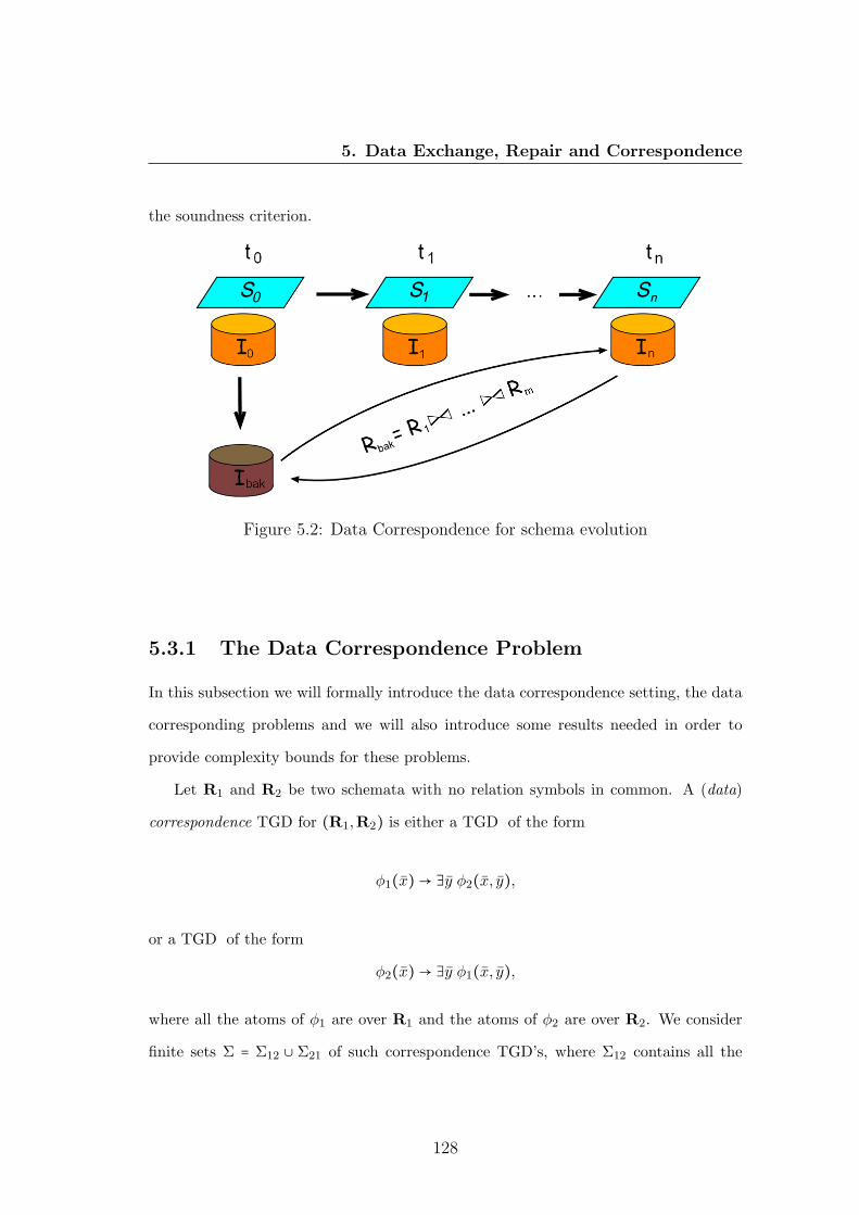
5. Data Exchange, Repair and Correspondence
the soundness criterion.
Figure 5.2: Data Correspondence for schema evolution
5.3.1 The Data Correspondence Problem
In this subsection we will formally introduce the data correspondence setting, the data
corresponding problems and we will also introduce some results needed in order to
provide complexity bounds for these problems.
Let R1 and R2 be two schemata with no relation symbols in common. A (data)
correspondence TGD for (R1,R2) is either a TGD of the form
φ1(x) → ∃y φ2(x, y),
or a TGD of the form
φ2(x) → ∃y φ1(x, y),
where all the atoms of φ1 are over R1 and the atoms of φ2 are over R2. We consider
finite sets Σ = Σ12 ∪ Σ21 of such correspondence TGD’s, where Σ12 contains all the
128

5. Data Exchange, Repair and Correspondence
TGD’s of the first form, and Σ21 the TGD’s of the second form. Note that Σ12 are
used to specify a data exchange mapping [26], where the source schema is R1 and the
target schema is R2.
A (data) correspondence mapping is as a triple of the form (R1,R2,Σ), where
Σ = Σ12 ∪Σ21 is a set of correspondence mappings for (R1,R2) as above. We say that
a ground instance (I1, I2) over (R1,R2) satisfies the setting if (I1, I2) ⊧ Σ.
Let (R1,R2,Σ) be a data correspondence setting, and (I1, I2) a ground instance
over (R1,R2). Then ⟨(I1, I2), (R1,R2,Σ)⟩ denotes an instance of the uniform-data
correspondence problem. For simplicity, we call it uniform correspondence problem. For
such an instance, usually simply denoted (I1, I2,Σ), there are three types of solutions,
namely: subset-solutions, superset-solutions, and ⊕-solutions.
Definition 32 Let (I1, I2,Σ) be an instance of the uniform data correspondence prob-
lem and (K1,K2) a ground instance over (R1,R2). If (K1,K2) satisfies Σ and K1 ∪
K2 ≠ ∅, we say that (K1,K2) is a
• subset-solution if (K1,K2) ⊆ (I1, I2) and (K1,K2) is maximal among the subsets
of (I1, I2) satisfying Σ;
• superset-solution if (K1,K2) ⊇ (I1, I2) and (K1,K2) is minimal among the su-
persets of (I1, I2) satisfying Σ;
• ⊕-solution if (K1,K2) is ≤(I1,I2)-minimal among the instances satisfying Σ,
where the notion of subset is extended to pair of sets as follows: (A,B) ⊆ (C,D)
iff A ⊆ C and B ⊆ D. Note, in the previous definition, that in all cases an instance
can have one or several solutions. Subset and ⊕-solutions might not exist, whereas
superset-solutions always do.
The non-uniform-data correspondence problem (shortly called the non-unform cor-
respondence problem) is similar to the uniform one, except that the instance I1 is kept
129

5. Data Exchange, Repair and Correspondence
fixed when looking for solutions. This has, among other things, the consequence that
not even superset-solutions are guaranteed to exist.
Definition 33 Let (I1, I2,Σ12 ∪ Σ21) be an instance of the non-uniform-data corre-
spondence problem and K2 a ground instance over R2. If (I1,K2) satisfies Σ, we say
that K2 is a
• subset-solution if K2 ⊆ I2 and K2 is maximal among the subsets of I2, such that
(I1,K2) satisfies Σ;
• superset-solution if K2 ⊇ I2 and K2 is minimal among the supersets of I2, such
that (I1,K2) satisfies Σ;
• ⊕-solution if K2 is ≤I2-minimal among the instances of R2, such that (I1,K2)
satisfies Σ.
Example 33 Consider schemata R1 = {R} and R1 = {S}. Consider also instance
(I1, I2) over schema (R1,R2), where I1 = {R(a, b),R(c, d)} and I2 = {S(c, a)}. Finally,
let Σ12 = {R(x, y) → ∃z S(x, z)} and Σ21 = {S(x, y), S(y, z) → R(x, z)}. Now consider
the following pairs of instances (we used square boxes as pair delimiter):
K11
R(c, d)
K12
S(c, a)
K21
R(a, b)R(c, d)R(c, b)
K22
S(c, a)R(a, b)
K31
R(a, b)
K32
S(a, d)
For the uniform correspondence problem (I1, I2,Σ12 ∪ Σ21), instance (K11 ,K1
2) is a
subset-solution; similarly, instance (K21 ,K2
2) is a superset-solution; and (K21 ,K2
2) is a
⊕-solution. In the case of uniform correspondence problem (I1, I2,Σ12 ∪Σ21), instance
J2 = {S(c, a), S(c, a)} is a superset-solution because (I1, J2) ⊧ Σ12 ∪ Σ21 and because
J2 = I2∪{S(a, d)}. We may also note that there does not exist a subset-solution for the
130

5. Data Exchange, Repair and Correspondence
non-uniform correspondence problem, following that all ⊕-solutions are the superset-
solutions.
Similarly to the data repair case, the above definitions give rise to classes of decision
problems that we will study in the next subsection. The first class is the existence of
solutions to the correspondence problem. While the second class is to check whether
a given instance is a solution. We note that Fuxman, Kolaitis, Miller and Tan [11]
have investigated, under the name of Peer Data Exchange, the existence of superset-
solutions to the non-uniform correspondence problem. However, they do not require
a solution to be minimal, which in fact leaves out an additional computational hurdle
similar to computing the core of a solution. In addition, it turns out that the uniform
correspondence problem can be seen as a special case of the problem of the repair
checking problem.
Lemma 6 Let (I1, I2,Σ1,Σ2) be an instance of the uniform-data correspondence prob-
lem and (K1,K2) a ground instance. Then (K1,K2) is a subset(superset, ⊕)-solution
to the uniform correspondence problem if and only if K1 ∪K2 is a subset (superset, ⊕,
respectively) repair of I1 ∪ I2 w.r.t. Σ1 ∪Σ2.
From this lemma it follows that the characterization used for the ⊕-solution in The-
orem 32 works for ⊕-uniform-data correspondence solutions as well. In case of solutions
to the non-uniform correspondence problem, we have a similar characterization.
Theorem 41 Let (I1, I2,Σ12,Σ21), with Σ = Σ12 ∪ Σ21, be an instance of the non-
uniform correspondence problem, and K2 an instance such that (I1,K2) ⊧ Σ. Then K2
is a ⊕-solution for (I1, I2,Σ12,Σ21) if and only if the following conditions are satisfied:
131

5. Data Exchange, Repair and Correspondence
1. For all Σ-satisfying homomorphism h with h(chasestdΣ (I1, I2 ∩K2)) ⊆ (I1,K2)
and all J2 ⊆ K2 with (I1, J2) ⊧ Σ and h(chasestdΣ (I1, I2 ∩K2)) ⊆ (I1, J2), it holds
that J2 = K2.
2. There does not exist a tuple t ∈ I2 ∖K2 and a Σ-satisfying homomorphism h with
J2 ⊆ (I2 ∪K2), s.t. (I1, J2) ⊧ Σ and h(chasestdΣ (I1, I2 ∩K2 ∪ {t})) ⊆ (I1, J2).
Proof: Suppose instance K2 is a ⊕-solution. As (I1,K2) ⊧ Σ, we have the result
of the chase, chasestdΣ (I1,K2) = (I1,K2). By Lemma 2 there then exists a homo-
morphism h such that h(chasestdΣ (I1, I2 ∩K2)) ⊆ (I1,K2). Toward a contradiction,
suppose that condition 1 is violated. This means that there exists an instance J2 such
that h(chasestdΣ (I1, I2 ∩K2)) ⊆ (I1, J2) ⊂ (I1,K2) and (I1, J2) ⊧ Σ. Then we have
(J2 ∖ I2) ⊂ (K2 ∖ I2) and, since (I1, I2 ∩K2) ⊆ chasestdΣ (I1, I2 ∩K2) and (I1, I2 ∩K2)
is a ground instance, we have that (I1, I2 ∩K2) ⊆ (I1, J2). As the two schemata are
distinct, it follows that (I2 ∩K2) ⊆ J2. Thus (I2 ∖ J2) ⊆ (I2 ∖K2) and J2 <I2 K2. But
this contradicts the assumption that K2 is a ⊕-solution. Therefore it must be that
J2 = K2, meaning that K2 satisfies condition 1.
Suppose then that condition 2 is violated and tuple t, Σ-satisfying homomorphism
h and instance J2 exist. Since for such a J2 we would have (I2 ∖ J2) ⊂ (I2 ∖ K2), it
would follow that J2 <I2 K2, contradicting the assumption that K2 is a ⊕-solution.
For the only if direction let K2 be an instance such that (I1,K2) ⊧ Σ and K2 satisfies
conditions 1 and 2. We need to show that K2 is ⊕-minimal. If this is not the case there
must be an instance J2, such that J2 <I2 K2 and (I1, J2) ⊧ Σ. Thus (J2∖I2) ⊆ (K2∖I2)
and (I2 ∖ J2) ⊆ (I2 ∖K2), and at least one of the inclusions is proper. Suppose first
that it were the case that (I2 ∖ J2) = (I2 ∖K2). Then we would have J2 ⊆ K2. So if
J2∖I2 were to be a proper subset of K ∖I2, it would necessarily be that J2 ⊂ K2. Since
(I2∩J2) = (I2∩K2), chasestdΣ (I1, I2 ∩ J2) = chasestd
Σ (I1, I2 ∩K2), and by Lemma 2 there
is a homomorphism h such that h(chasestdΣ (I1, I2 ∩ J)) ⊆ chasestd
Σ (I1, J2) = (I1, J2).
132

5. Data Exchange, Repair and Correspondence
But then it would hold that h(chasestdΣ (I1, I2 ∩ J)) ⊆ (I1, J2) ⊂ (I1,K2), contradicting
condition 1.
On the other hand, if it were the case that (I2 ∖ J2) ⊂ (I2 ∖ K2), we would find
a tuple t ∈ (I2 ∩ J2) ∖ (I2 ∩ K2), and Lemma 2 would give us a homomorphism h,
such that h(chasestdΣ (I1, I2 ∩K ∪ {t})) ⊆ (I1, J2) ⊂ (I1, I2 ∪K2), a contradiction to the
assumption that K2 satisfies condition 2∎
In the following subsection we will consider the following decisions problems for
the uniform and non-uniform correspondence cases. Note that, even if by Lemma 6
the uniform correspondence problem can be reduced to a corresponding data repair
problem, the reverse does not always hold; as in data correspondence problem we
consider only correspondence TGD’s, which is not the case in data repair.
Definition 34 Decision problems considered:
• Existence-of-Solution(Σ12 ∪Σ21, subset/superset/⊕,uniform/non-uniform)
The input is (I1, I2) and the question is whether the uniform/non-uniform cor-
respondence problem (I1, I2,Σ12 ∪Σ21) has a subset/superset/⊕-solution;
• Solution-Checking(Σ12 ∪Σ21, subset/superset/⊕,uniform/non-uniform)
The input is pairs of instances (I1, I2) and (K1,K2) and the question is whether
the (K1,K2) is a subset/superset/⊕-solution for the uniform/non-uniform cor-
respondence problem (I1, I2,Σ12 ∪Σ21).
5.3.2 Complexity Results
In this section we are going over all previously defined decision problems using different
classes of dependencies and investigate the corresponding data complexity results. The
Existence-of-Solution(Σ, superset/⊕, uniform) decision problem is a non-problem
133

5. Data Exchange, Repair and Correspondence
for the class of weakly acyclic set of TGD’s, since superset-solutions always exist (recall
that no denial constraints are present). In this subsection we shall see that the uniform
version of the correspondence problem is coNP-complete for weakly acyclic TGD’s and
for all types of solutions. However, using homomorphism techniques, we are able to
show that the non-uniform version of the problem is polynomial for subset and superset-
solutions. Somewhat surprisingly then it turns out that the non-uniform version is
coNP-complete for ⊕-solutions.
Let us first start considering the problems when Σ is specified by a weakly acyclic
set of TGD’s.
Corollary 6 Let Σ = Σ12 ∪ Σ21 be a set of weakly acyclic TGD’s. Then the problem
Existence-of-Solution(Σ, subset, uniform) can be solved in polynomial time.
Proof: Follows directly from Lemma 6∎
Theorem 42 Let Σ = Σ12 ∪Σ21 be a set of weakly acyclic TGD’s. Then the problem
Solution-Checking(Σ, subset, non-uniform) can be solved in polynomial time.
Proof: Let (I1, I2) be an instance, Then instance K2 ⊆ I2 is a subset-solution for
(I1, I2,Σ12,Σ21), if (I1,K2) ⊧ Σ and there does not exist an instance J2 such that
K2 ⊂ J2 ⊆ I2 and (I1, J2) ⊧ Σ. The test (I1,K2) ⊧ Σ can be done in space logarithmic
in the size of (I1,K2). It is obvious that J2, as mentioned above, does exist iff there is a
tuple t ∈ I2∖K2 and homomorphism h such that h(chasestdΣ21
(K2 ∪ {t})) ⊆ I1. It follows
from Theorem 33 that the existence of such a homomorphism h can be determined in
polynomial time in the size of I1. The chase with Σ21 and the homomorphism test is
repeated for each tuple in I2 ∖K2. The whole process thus runs in polynomial time in
the size of ∣I1∣ + ∣I2∣∎
Theorem 43 Let Σ = Σ12 ∪Σ21 be a set of weakly acyclic TGD’s. Then the problem
Solution-Checking(Σ, superset, non-uniform) can be solved in polynomial time.
134

5. Data Exchange, Repair and Correspondence
Proof: Consider the non-uniform correspondence problem (I1, I2,Σ). And also consider
K2 the candidate-solution. First test if (I1,K2) ⊧ Σ. If so, look for a tuple t ∈ K2 ∖ I2
and a homomorphism h from chasestdΣ12
(I1) to K2∖{t}. By Theorem 33 this process can
be carried out in polynomial time in the size of (I1,K2). Evidently, if such a tuple t and
homomorphism h are found, K2 is not a superset-solution, since then (I1,K2∖{t}) ⊧ Σ,
meaning that K2 is not minimal. If no tuple t and homomorphism h is found, K2 is
obviously minimal∎
We just saw that for the non-uniform correspondence problem, checking whether an
instance is a subset-solution or a superset-solution is polynomial. If we allow a solution
to be in part a subset, and in part a superset the problem becomes coNP-complete.
Theorem 44 Let Σ = Σ12 ∪ Σ21 be a set of tuple generating dependencies. Then the
problem Solution-Checking(Σ,⊕,non-uniform) is in coNP, and is coNP-hard even
for weakly acyclic TGD’s.
Proof: Let (I1, I2,Σ) be the non-uniform correspondence problem and K2 the candidate
solution. To see that the problem is in coNP, consider the complementary problem:
Does there exist an instance J2 such that (I1, J2) ⊧ Σ, and J2 <I2 K2? This problem
is clearly in NP, since we can guess J2 and then check in logarithmic space whether
(I2, J2) ⊧ Σ.
For the lower bound we will reduce the Positive 1-In-3-SAT problem to the
⊕-repair checking one. The Positive 1-In-3-SAT problem asks whether a set of
disjunctive clauses, each having three positive variables, is satisfiable with a truth
assignment that makes exactly one variable in each clause true. This problem is known
to be NP-complete.
We consider the schema (R1,R2), where R1 = {P,E,V,F} and R2 = {T,S,D}. Let
Σ12 consist of the following dependencies:
135

5. Data Exchange, Repair and Correspondence
P (x, y, z) → ∃u, v,w ∶ T (x,u), T (y, v), T (z,w), S(u, v,w) (5.2)
F (u, v,w, u′, v′,w′) → D(u, v,w, u′, v′,w′) (5.3)
and Σ21 consist of
T (x,u), T (x,u′) → E(u,u′) (5.4)
S(u, v,w), S(u′, v′,w′),D(u, v,w, u′, v′,w′) → V (u, v,w). (5.5)
Note that Σ12 ∪Σ21 is a weakly acyclic set.
Given an instance P of the Positive 1-In-3-SAT problem we construct I1 as
P I1 = {(x, y, z) ∶ x ∨ y ∨ z is a clause in P}
EI1 = {(0,1), (1,0)}
V I1 = {(0,0,1), (0,1,0) (1,0,0)}
F I1 = {(u, v,w) (u′, v′,w′) ∶ u, v,w, u′, v′,w′ ∈ {1,0}, (u, v,w) ≠ (u′, v′.w′)}
and I2 as
T I2 = {(x,0) ∶ x variable in P}
SI2 = {(0,0,1), (0,1,0), (1,0,0)}
DI2 = F I1 .
Finally, let K2 be
TK2 = {(x,1) ∶ x is a variable in P}
SK2 = {(1,1,1)}
DK2 = DI2 .
It is straightforward to verify that (I1,K2) ⊧ Σ. The reduction clearly being polyno-
mial, it remains only to prove that there exists a truth assignment for P making exactly
136
5. Data Exchange, Repair and Correspondence
one variable in each clause true, if and only if K2 is not a ⊕-repair.
Suppose that there exists such a Positive 1-In-3 truth assignment making P true.
Let this truth assignment be represented by a mapping ν from the variables of P to
{0,1}. Consider then an instance J2 with
T J2 = {(x, ν(x)) ∶ x is a variable in P}
SJ2 = {(0,0,1), (0,1,0), (1,0,0)}
DJ2 = DK2 .
It is easy to verify that (I1, J2) ⊧ Σ and that J2 <I2 K2. Thus K2 is not a ⊕-repair.
For the other direction, suppose that there does not exist a Positive 1-In-3 truth
assignment making P true. Let us try to construct an instance J2 such that (I1, J2) ⊧ Σ
and J2 <I2 K2, by manipulating K2 to become ⊕-closer to I2.
First we note that dependencies 5.2 and 5.4 force the interpretation of T to contain
exactly a truth assignment for each variable and that dependency 5.3 blocks us from
deleting tuples from DK2 .
We could make K2 closer to I2 by replacing some tuples (x,1) in TK2 with (x,0).
But then, in order to satisfy dependency 5.2, we would have to replace the tuple
(1,1,1) ∈ SK2 with at least one tuple containing at least one ’0’. Suppose first that
there were only one new tuple and that this tuple would contain only one ’0’. This
would make the resulting instance ≤I2-incomparable with K2. To avoid this, we could
leave tuple (1,1,1) in the interpretation of S. But then the interpretation of S would
contain at least two tuples. So, in any case, dependency 5.5 will be triggered, forcing the
interpretation of S to contain only tuples from V I1 . We would then have constructed
a Positive 1-In-3 truth assignment for P in the interpretation of T . We have now
exhausted all possibilities to improve the solution K2 and can therefore conclude that
K2 indeed is a ⊕-solution∎
137

5. Data Exchange, Repair and Correspondence
The next theorem shows that the result of Afrati and Kolaitis [4] can actually be
sharpened to also hold for subset-solution checking for the correspondence problem.
Theorem 45 There are weakly acyclic sets Σ = Σ12 ∪ Σ21 of TGD’s such that the
problem Solution-Checking(Σ, subset,uniform) is coNP-complete.
Proof: Let (I1, I2,Σ) be a uniform correspondence problem and (K1,K2) a candi-
date solution. As before, in order to see that the problem is in coNP, we will con-
sider complementary problem of deciding if there exists an instance (J1, J2) such that
(K1,K2) ⊂ (J1, J2) ⊆ (I1, I2) and (J1, J2) ⊧ Σ. This problem is clearly in sf NP as some
may guess such an instance (J1, J2) and using a polynomial verifier check if (J1, J2) ⊧ Σ.
For the lower bound we will reduce the Positive 1-In-3-SAT to the subset-solution
checking problem.
We consider the schemata R1 = {A,P,E} and R2 = {T,S,D}. The dependencies
considered are Σ = Σ12 ∪Σ21, where Σ12 consists of the following:
A(n), P (x, y, z) → ∃u, v,w ∶ T (x,u), T (y, v), T (z,w), S(u, v,w)
and Σ21 consists of:
T (x,u), T (x,u′),D(u,u′) → E(u)T (x,u) → A(x)
Now we construct I1 from the instance P of the Positive 1-In-3-SAT to be as:
AI1 = {(x) ∶ x is a variable in P}P I1 = {(x, y, z) ∶ x ∨ y ∨ z is a clause in P}EI1 = ∅
and instance I2 as
138
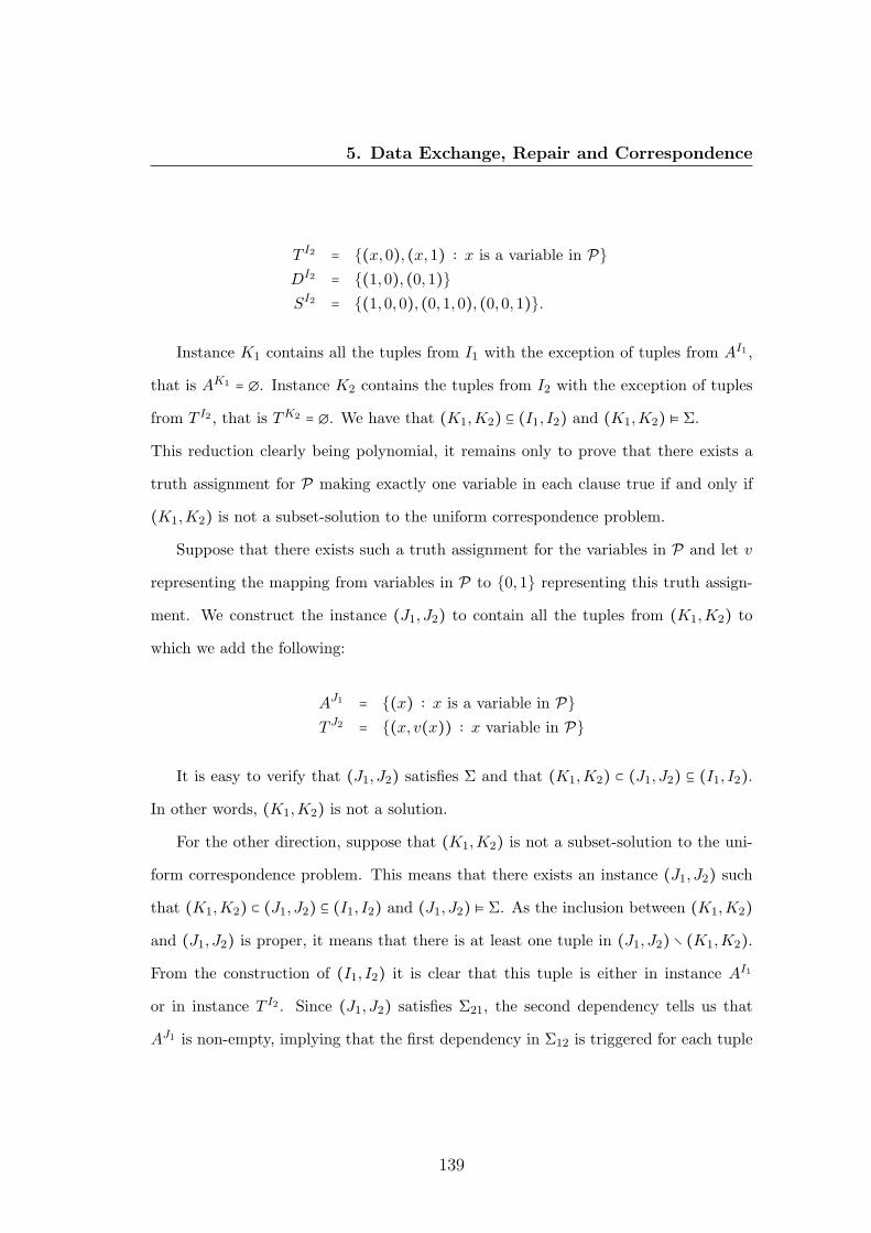
5. Data Exchange, Repair and Correspondence
T I2 = {(x,0), (x,1) ∶ x is a variable in P}DI2 = {(1,0), (0,1)}SI2 = {(1,0,0), (0,1,0), (0,0,1)}.
Instance K1 contains all the tuples from I1 with the exception of tuples from AI1 ,
that is AK1 = ∅. Instance K2 contains the tuples from I2 with the exception of tuples
from T I2 , that is TK2 = ∅. We have that (K1,K2) ⊆ (I1, I2) and (K1,K2) ⊧ Σ.
This reduction clearly being polynomial, it remains only to prove that there exists a
truth assignment for P making exactly one variable in each clause true if and only if
(K1,K2) is not a subset-solution to the uniform correspondence problem.
Suppose that there exists such a truth assignment for the variables in P and let v
representing the mapping from variables in P to {0,1} representing this truth assign-
ment. We construct the instance (J1, J2) to contain all the tuples from (K1,K2) to
which we add the following:
AJ1 = {(x) ∶ x is a variable in P}T J2 = {(x, v(x)) ∶ x variable in P}
It is easy to verify that (J1, J2) satisfies Σ and that (K1,K2) ⊂ (J1, J2) ⊆ (I1, I2).
In other words, (K1,K2) is not a solution.
For the other direction, suppose that (K1,K2) is not a subset-solution to the uni-
form correspondence problem. This means that there exists an instance (J1, J2) such
that (K1,K2) ⊂ (J1, J2) ⊆ (I1, I2) and (J1, J2) ⊧ Σ. As the inclusion between (K1,K2)
and (J1, J2) is proper, it means that there is at least one tuple in (J1, J2) ∖ (K1,K2).
From the construction of (I1, I2) it is clear that this tuple is either in instance AI1
or in instance T I2 . Since (J1, J2) satisfies Σ21, the second dependency tells us that
AJ1 is non-empty, implying that the first dependency in Σ12 is triggered for each tuple
139

5. Data Exchange, Repair and Correspondence
(x, y, z) in P J1 , thus forcing each variable to have valuation (0 or 1) in T J2 , and by the
tuples in SJ2 , each ”clause” must have exactly one variable valuated to true. The first
dependency in Σ21 together with the tuples in DJ2 ensure that each variable gets only
one value in T J2 . Clearly now the values recorded in T J2 constitute a desired truth
assignment of P∎
From Lemma 6 and Theorem 45 we get
Corollary 7 There is a weakly acyclic set set Σ = Σ12 ∪Σ21 of TGD’s such that the
Solution-Checking(Σ,⊕,uniform) problem is coNP-complete.
Let us now turn our attention to the superset problem for the uniform correspon-
dence.
Theorem 46 There is a weakly acyclic set Σ = Σ12 ∪ Σ21, of TGD’s, such that the
problem Solution-Checking(Σ, superset, uniform) is coNP-complete.
Proof: The upper bound follows directly from Lemma 6 and Theorem 37.
For the lower bound we will use a reduction from the same Positive 1-In-3-
SAT problem with a set of dependencies slightly modified from the proof of Theorem
37. Consider the schemata R1 = {P,R,E} and R2 = {T,S,D} together with the
dependencies Σ = Σ12 ∪Σ21, with Σ12 containing the following set of dependencies:
P (x, y, z) → ∃u, v,w T (x,u), T (y, v), T (z,w), S(u, v,w) (5.6)
R(x,u),E(y) → ∃u′ T (x,u′),D(u,u′). (5.7)
and Σ21 containing:
T (x,u), T (x,u′),D(u,u′) → ∃y E(y) (5.8)
T (x,u) → R(x,u). (5.9)
140

5. Data Exchange, Repair and Correspondence
Let P be an instance of the Positive 1-In-3-SAT problem. Also consider (I1, I2)
as an instance and (K1,K2) a candidate superset-solution for the corresponding uni-
form correspondence problem. Similarly to the previous proofs, we will consider the
complementary problem of deciding if there exists an instance (J1, J2) such that the
following holds (I1, I2) ⊆ (J1, J2) ⊂ (K1,K2) and (J1, J2) ⊧ Σ.
Instance I1 is constructed from instance P in the following way:
P I1 = {(x, y, z) ∶ x ∨ y ∨ z is a clause in P}
RI1 = ∅
EI1 = ∅
Instance I2 is built to contain the following constant tuples:
T I2 = ∅
SI2 = {(1,0,0), (0,1,0), (0,0,1)}
DI2 = {(1,0), (0,1)}
The candidate superset-solution (K1,K2) is also constructed from instance P , with
K1 containing the following tuples:
PK1 = {(x, y, z) ∶ x ∨ y ∨ z is a clause in P}
RK1 = {(x,0), (x,1) ∶ x variable in P}
EK1 = {(0)}
We consider the following tuples for K2:
TK2 = {(x,0), (x,1) ∶ x variable in P}
SK2 = {(1,0,0), (0,1,0), (0,0,1)}
DK2 = {(1,0), (0,1)}
This reduction is clearly polynomial and we also have that (I1, I2) ⊆ (K1,K2) and
141
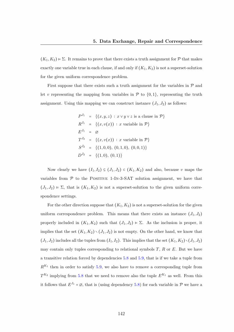
5. Data Exchange, Repair and Correspondence
(K1,K2) ⊧ Σ. It remains to prove that there exists a truth assignment for P that makes
exactly one variable true in each clause, if and only if (K1,K2) is not a superset-solution
for the given uniform correspondence problem.
First suppose that there exists such a truth assignment for the variables in P and
let v representing the mapping from variables in P to {0,1}, representing the truth
assignment. Using this mapping we can construct instance (J1, J2) as follows:
P J1 = {(x, y, z) ∶ x ∨ y ∨ z is a clause in P}
RJ1 = {(x, v(x)) ∶ x variable in P}
EJ1 = ∅
T J2 = {(x, v(x)) ∶ x variable in P}
SJ2 = {(1,0,0), (0,1,0), (0,0,1)}
DJ2 = {(1,0), (0,1)}
Now clearly we have (I1, I2) ⊆ (J1, J2) ⊂ (K1,K2) and also, because v maps the
variables from P to the Positive 1-In-3-SAT solution assignment, we have that
(J1, J2) ⊧ Σ, that is (K1,K2) is not a superset-solution to the given uniform corre-
spondence settings.
For the other direction suppose that (K1,K2) is not a superset-solution for the given
uniform correspondence problem. This means that there exists an instance (J1, J2)
properly included in (K1,K2) such that (J1, J2) ⊧ Σ. As the inclusion is proper, it
implies that the set (K1,K2)∖(J1, J2) is not empty. On the other hand, we know that
(J1, J2) includes all the tuples from (I1, I2). This implies that the set (K1,K2)∖(J1, J2)
may contain only tuples corresponding to relational symbols T , R or E. But we have
a transitive relation forced by dependencies 5.8 and 5.9, that is if we take a tuple from
RK1 then in order to satisfy 5.9, we also have to remove a corresponding tuple from
TK2 implying from 5.8 that we need to remove also the tuple EK1 as well. From this
it follows that EJ1 = ∅, that is (using dependency 5.8) for each variable in P we have a
142

5. Data Exchange, Repair and Correspondence
single truth assignment given by instance T J2 . But now from dependency 5.6, it follows
that for each clause in P we have only one variable evaluated to true. Consequently the
assignment given by the instance T J2 is a solution for Positive 1-In-3-SAT problem
over instance P∎
Let us now consider the existence of the solution problem for the non-uniform corre-
spondence settings. For this, as it will be proved, all the three cases subset/superset/⊕
are intractable for general weakly acyclic set of tuple generating dependencies.
Theorem 47 There is a weakly acyclic set Σ = Σ12 ∪ Σ21 such that the problem
Existence-of-Solution(Σ, subset, non-uniform) is NP-complete.
Proof: Let (I1, I2,Σ) be a non-uniform correspondence problem. We need to decide if
there exists an instance J such that J ⊆ I2 and (I1, J) ⊧ Σ. This problem is clearly in
NP as some may guess such an instance and the verifier is polynomial.
For the lower bound we will use the same Positive 1-In-3-SAT problem to be
reduced to an existence subset-solution problem over a uniform correspondence setting.
For this let’s consider the schemata R1 = {P,V,E} and R2 = {T,S,D}. Let us also
consider the following set of dependencies for Σ12:
P (x, y, z) → ∃u, v,w T (x,u), T (y, v), T (z,w), S(u, v,w) (5.10)
V (u,u′) → U(u,u′) (5.11)
and for Σ21 the following set of dependencies:
T (x,u), T (x,u′),D(u,u′) → E(u) (5.12)
Now, given an instance P of the Positive 1-In-3-SAT problem, we construct
instance I1 as:
143

5. Data Exchange, Repair and Correspondence
P I1 = {(x, y, z) ∶ x ∨ y ∨ z is a clause in P}
V I1 = {(0,1), (1,0)}
EI1 = ∅
and instance I2 as:
T I2 = {(x,0), (x,1) ∶ x variable in P}
DI2 = {(1,0), (0,1)}
SI2 = {(1,0,0), (0,1,0), (0,0,1)}.
The reduction is clearly polynomial. It remains only to prove that there exists a
truth assignment for P making exactly one variable in each clause true if and only
if there exists a subset-solution for the non-uniform correspondence problem given by
(I1, I2,Σ12,Σ21).
First let us suppose that there exists a solution for the Positive 1-In-3-SAT
problem over instance P . Consider v to be the mapping from variables in P to {0,1}
given by the solution. We can now construct the following instance J over schema R2:
T J = {(x, v(x)) ∶ x variable in P}
DJ = {(1,0), (0,1)}
SJ = {(1,0,0), (0,1,0), (0,0,1)}.
It is clear that J ⊆ I2 and (I1, J) ⊧ Σ. That is if there exists a Positive 1-In-3-
SAT truth assignment for instance P , then there exists a subset-solution for the created
non-uniform correspondence problem.
For the other direction, let us suppose that for the given non-uniform correspon-
dence instance (I1, I2) there exists an instance J over R2 such that J ⊆ I2 and
(I1, J) ⊧ Σ. From this last assumption it follows that (by using dependency 5.10)
144

5. Data Exchange, Repair and Correspondence
there exist truth and assignment for each variable in P , given by T J , such that it
makes true exactly one variable from each clause. On the other hand, dependency 5.11
ensures that the instance DJ contains the same tuples as V I1 . This ensures, by using
dependency 5.12, that there exists a unique assignment for each variable. From these
it follows that the assignment given by instance T J is a Positive 1-In-3-SAT truth
assignment for instance P∎
We get the same result if we consider the problem of the existence for a superset-
solution over a non-uniform correspondence setting.
Theorem 48 There is a set Σ = Σ12 ∪ Σ21 of weakly acyclic TGD’s such that the
problem Existence-of-Solution(Σ, superset, non-uniform) is NP-complete.
Proof: Let (I1, I2) be an instance. The problem is to decide if there exists an instance
J such that J ⊇ I2 and (I1, J) ⊧ Σ. This problem is clearly in NP as some may guess
such an instance over a finite domain given by the domain of dom(I1) ∪ dom(I2). Also
the verifier is polynomial.
Again, for the lower bound we will use Positive 1-In-3-SAT problem to be reduced
to an existence subset-solution problem over a uniform correspondence setting. For this
let’s consider the schemata R1 = {P,V,E} and R2 = {T,S,D}. Let us also consider the
following set of dependencies for Σ12:
P (x, y, z) → ∃u, v,w T (x,u), T (y, v), T (z,w), S(u, v,w) (5.13)
and for Σ21 the following dependencies:
T (x,u), T (x,u′),D(u,u′) → E(u,u, u) (5.14)
D(u, v) → V (u, v) (5.15)
S(u, v,w) → E(u, v,w). (5.16)
145
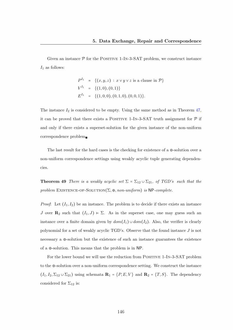
5. Data Exchange, Repair and Correspondence
Given an instance P for the Positive 1-In-3-SAT problem, we construct instance
I1 as follows:
P I1 = {(x, y, z) ∶ x ∨ y ∨ z is a clause in P}
V I1 = {(1,0), (0,1)}
EI1 = {(1,0,0), (0,1,0), (0,0,1)}.
The instance I2 is considered to be empty. Using the same method as in Theorem 47,
it can be proved that there exists a Positive 1-In-3-SAT truth assignment for P if
and only if there exists a superset-solution for the given instance of the non-uniform
correspondence problem∎
The last result for the hard cases is the checking for existence of a ⊕-solution over a
non-uniform correspondence settings using weakly acyclic tuple generating dependen-
cies.
Theorem 49 There is a weakly acyclic set Σ = Σ12 ∪ Σ21, of TGD’s such that the
problem Existence-of-Solution(Σ,⊕,non-uniform) is NP-complete.
Proof: Let (I1, I2) be an instance. The problem is to decide if there exists an instance
J over R2 such that (I1, J) ⊧ Σ. As in the superset case, one may guess such an
instance over a finite domain given by dom(I1) ∪ dom(I2). Also, the verifier is clearly
polynomial for a set of weakly acyclic TGD’s. Observe that the found instance J is not
necessary a ⊕-solution but the existence of such an instance guarantees the existence
of a ⊕-solution. This means that the problem is in NP.
For the lower bound we will use the reduction from Positive 1-In-3-SAT problem
to the ⊕-solution over a non-uniform correspondence setting. We construct the instance
(I1, I2,Σ12 ∪ Σ21) using schemata R1 = {P,E,V } and R2 = {T,S}. The dependency
considered for Σ12 is:
146
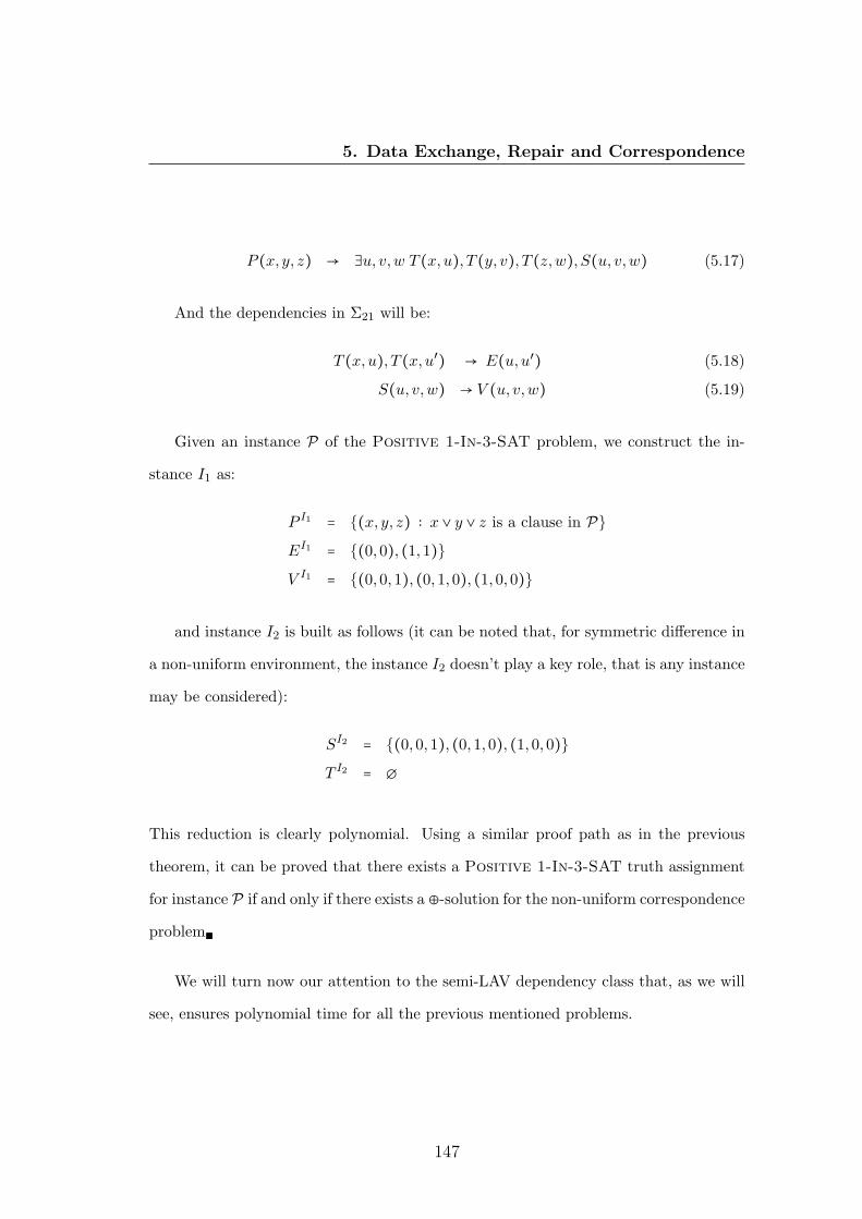
5. Data Exchange, Repair and Correspondence
P (x, y, z) → ∃u, v,w T (x,u), T (y, v), T (z,w), S(u, v,w) (5.17)
And the dependencies in Σ21 will be:
T (x,u), T (x,u′) → E(u,u′) (5.18)
S(u, v,w) → V (u, v,w) (5.19)
Given an instance P of the Positive 1-In-3-SAT problem, we construct the in-
stance I1 as:
P I1 = {(x, y, z) ∶ x ∨ y ∨ z is a clause in P}
EI1 = {(0,0), (1,1)}
V I1 = {(0,0,1), (0,1,0), (1,0,0)}
and instance I2 is built as follows (it can be noted that, for symmetric difference in
a non-uniform environment, the instance I2 doesn’t play a key role, that is any instance
may be considered):
SI2 = {(0,0,1), (0,1,0), (1,0,0)}
T I2 = ∅
This reduction is clearly polynomial. Using a similar proof path as in the previous
theorem, it can be proved that there exists a Positive 1-In-3-SAT truth assignment
for instance P if and only if there exists a ⊕-solution for the non-uniform correspondence
problem∎
We will turn now our attention to the semi-LAV dependency class that, as we will
see, ensures polynomial time for all the previous mentioned problems.
147

5. Data Exchange, Repair and Correspondence
Theorem 50 Let Σ = Σ12 ∪ Σ21 be a set of semi-LAV TGD’s. Then the problem
Existence-of-Solution(Σ, subset, non-uniform) can be solved in polynomial time.
Proof: Let (I1, I2,Σ12 ∪ Σ21) be an instance of the non-uniform correspondence. In
order to determine if there exists an instance K2 ⊆ I2, such that (I1,K2) ⊧ Σ, it
suffices to determine if there exists a Σ-satisfying homomorphism from chasestdΣ (I1,∅)
to (I1, I2). Since Σ is a set of semi-LAV TGD’s, it follows from Theorems 39 and 33
that the latter condition can be tested in polynomial time∎
Theorem 51 Let Σ = Σ12 ∪ Σ21 be a set of semi-LAV TGD’s. Then the problem
Existence-of-Solution(Σ, superset,non-uniform) is polynomial.
Proof: Let (I1, I2,Σ12∪Σ21) be an instance of the non-uniform correspondence problem.
First, compute (K1,K2) = chasestdΣ (I1, I2). Then, search for a homomorphism h such
that h(K1) ⊆ I1 and (h(K1), h(K2)) ⊧ Σ. The crucial point is that (K1,K2) has
bounded blocksize, since Σ is semi-LAV∎
Theorem 52 Let Σ = Σ12 ∪Σ21 be a set of semi-LAV dependencies. Then the problem
Existence-of-Solution(Σ,⊕,non-uniform) is polynomial.
Proof: Search for a homomorphism h, such that (I1, h(chasestdΣ12
(I1))) ⊧ Σ. From
Theorem 39 we know that we can find this in polynomial time∎
From Theorem 40 we conclude the following corollary:
Corollary 8 Let Σ = Σ12 ∪ Σ21 be a set of semi-LAV dependencies. The problems
Solution-Checking(Σ, subset/superset/⊕, uniform) can be solved in polynomial time.
Proof: Follows directly from Lemma 6 and Theorem 40. ∎
148

5. Data Exchange, Repair and Correspondence
Theorem 53 Let Σ be a set of semi-LAV tuple generating dependencies. Then the
problems Solution-Checking(Σ, subset/superset/⊕, non-uniform) are polynomial.
Proof: The subset/superset cases follow directly from Theorems 42 and 43 respectively.
In the ⊕-case we need to check if an instance K is a ⊕-solution for the non-uniform
correspondence problem of (I1, I2) w.r.t. Σ = Σ12 ∪ Σ21. First, test if K ⊧ Σ. If
so, K is indeed a ⊕-solution for the non-uniform correspondence problem if and only
if both conditions in Theorem 41 are fulfilled. Since Σ is semi-LAV, the required
homomorphism tests can be done in polynomial time, as per Theorem 39∎
We can now conclude this section with two tables summarizing the data complexity
results for the correspondence solution-existence and for the correspondence solution-
check problems under different dependency classes.
Existence unif. corr. sol. non-unif. corr. sol. non-unif. corr. sol.
Σ weakly acyc. weakly acyc. semi-LAV
subset P Cor. 6 NPC Thrm. 47 P Thrm. 50
superset - NPC Thrm. 47 P Thrm. 51
⊕ - NPC Thrm. 47 P Thrm. 52
Figure 5.3: Data complexity for solution-existence problem
Solution uniform uniform non-uniform non-uniform
Check Σ weakly acyc. semi-LAV weakly acyc. semi-LAV
subset coNPC Thrm. 45 P Thrm. 53 P Thrm. 42 P Thrm. 42
superset coNPC Thrm. 45 P Thrm. 53 P Thrm. 43 P Thrm. 43
⊕ coNPC Thrm. 45 P Thrm. 53 coNPC Thrm. 44 P Thrm. 53
Figure 5.4: Data complexity for the solution-check problem
149

Chapter 6
Closed World Chasing
In Chapter 5 we studied the chase procedure applicability in Data Exchange, Data
Repair and Data Correspondence problems. In Section 5.1 dedicated to data exchange,
we saw that the chase procedure could be used to materialize a “universal solution“ on
the target that may be used, after all, to get certain answers to any UCQ query. In
order to deal with a larger class of queries, Deutsch Nash and Remmel [23] introduced
the extended core chase to materialize on the target a set of universal solutions which
could answer a more larger class of queries, namely UCQ¬,≠. The semantics for certain
query answering in both cases is closed to the left and open to the right, that is the
source instance is considered closed, but the target instance open. As pointed out by
Libkin in [54], the tacit open world assumption creates anomalies in the (first order)
query evaluation even in the simplest data exchange setting where the target is declared
to be a copy of the source. To see this anomaly introduced by the open world semantics,
consider the following example:
Example 34 Recall the data exchange mapping M without target dependencies, from
Example 29, that simply copies the source instance to the target. Thus, as one may
150

6. Close World Chasing
expect, the certain answer to queries over the source instance should return the same
result when running the similar query on the materialized target instance. Consider
mapping M = ({R},{R′},Σst,∅) with Σst = {R(x, y) → R′(x, y)}. Using the extended
core-chase algorithm presented in Section 3.2 with source instance I = {R(a, b)}, we get
J = {J1, J2, J3, J4, J5, J6, J7, J8} as the universal solution set materialized on the target,
where the instances J1 to J8 are tabularly represented as follows:
J1
R′(a, b)
J2
R′(a, b)R′(a, a)
J3
R′(a, b)R′(b, b)
J4
R′(a, b)R′(a, a)R′(b, b)
J5
R′(a, b)R′(b, a)
J6
R′(a, b)R′(a, a)R′(b, a)
J7
R′(a, b)R′(b, b)R′(b, a)
J8
R′(a, b)R′(a, a)R′(b, b)R′(b, a)
Considering the boolean UCQ¬ query over the target schema q′ ← R′(x, y) ∧ ¬R′(x,x),
the certain answer for q′ over the materialized target universal set J is false. On the
other hand, running the query q ← R(x, y) ∧ ¬R(x,x) over the source instance we get
the certain answer true.
Moreover, even under the open world (OWA) semantics, the universal solution set
returned by the extended core chase is not suitable to be used to answer arbitrary FO
queries, as it is shown in the following example:
Example 35 Consider data exchange mapping M = ({R},{S,T},{R(x) → S(x)},∅).
Then consider source instance I = {R(a)} and the boolean query over the target instance
q ← T (x) → S(x) (note that query q is not an UCQ¬,≠, thus not contradicting the results
from [23]). Clearly, if one may use an open world assumption on the target, the instance
151
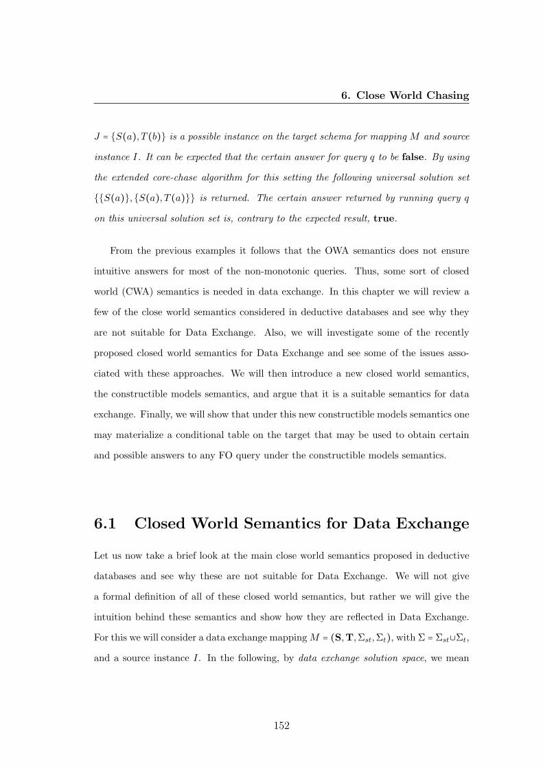
6. Close World Chasing
J = {S(a), T (b)} is a possible instance on the target schema for mapping M and source
instance I. It can be expected that the certain answer for query q to be false. By using
the extended core-chase algorithm for this setting the following universal solution set
{{S(a)},{S(a), T (a)}} is returned. The certain answer returned by running query q
on this universal solution set is, contrary to the expected result, true.
From the previous examples it follows that the OWA semantics does not ensure
intuitive answers for most of the non-monotonic queries. Thus, some sort of closed
world (CWA) semantics is needed in data exchange. In this chapter we will review a
few of the close world semantics considered in deductive databases and see why they
are not suitable for Data Exchange. Also, we will investigate some of the recently
proposed closed world semantics for Data Exchange and see some of the issues asso-
ciated with these approaches. We will then introduce a new closed world semantics,
the constructible models semantics, and argue that it is a suitable semantics for data
exchange. Finally, we will show that under this new constructible models semantics one
may materialize a conditional table on the target that may be used to obtain certain
and possible answers to any FO query under the constructible models semantics.
6.1 Closed World Semantics for Data Exchange
Let us now take a brief look at the main close world semantics proposed in deductive
databases and see why these are not suitable for Data Exchange. We will not give
a formal definition of all of these closed world semantics, but rather we will give the
intuition behind these semantics and show how they are reflected in Data Exchange.
For this we will consider a data exchange mapping M = (S,T,Σst,Σt), with Σ = Σst∪Σt,
and a source instance I. In the following, by data exchange solution space, we mean
152
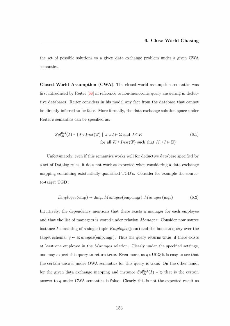
6. Close World Chasing
the set of possible solutions to a given data exchange problem under a given CWA
semantics.
Closed World Assumption (CWA). The closed world assumption semantics was
first introduced by Reiter [68] in reference to non-monotonic query answering in deduc-
tive databases. Reiter considers in his model any fact from the database that cannot
be directly inferred to be false. More formally, the data exchange solution space under
Reiter’s semantics can be specified as:
SolCWAM (I) = {J ∈ Inst(T) ∣ J ∪ I ⊧ Σ and J ⊆ K (6.1)
for all K ∈ Inst(T) such that K ∪ I ⊧ Σ}
Unfortunately, even if this semantics works well for deductive database specified by
a set of Datalog rules, it does not work as expected when considering a data exchange
mapping containing existentially quantified TGD’s. Consider for example the source-
to-target TGD :
Employee(emp) → ∃mgr Manages(emp,mgr),Manager(mgr) (6.2)
Intuitively, the dependency mentions that there exists a manager for each employee
and that the list of managers is stored under relation Manager. Consider now source
instance I consisting of a single tuple Employee(john) and the boolean query over the
target schema: q ← Manages(emp,mgr). Thus the query returns true if there exists
at least one employee in the Manages relation. Clearly under the specified settings,
one may expect this query to return true. Even more, as q ∈ UCQ it is easy to see that
the certain answer under OWA semantics for this query is true. On the other hand,
for the given data exchange mapping and instance SolCWAM (I) = ∅ that is the certain
answer to q under CWA semantics is false. Clearly this is not the expected result as
153

6. Close World Chasing
the given dependency specifies that there needs to exists at least one manager for each
employee. From this we can conclude that the CWA semantics is not a good approach
for data exchange mappings specified by existential TGD’s.
Generalized Closed World Assumption (GCWA). As the name suggests it,
GCWA semantics, introduced by Minker [66], generalizes CWA such that a data ex-
change solution under this semantics needs not to be a subset of each model but to
be a subset of some union of subset minimal models. Before presenting the solution
space for data exchange under GCWA semantics, let us introduce the notion of subset
minimality w.r.t. a set of dependencies Σ:
⊆min (M,I) = {J ∈ Inst(T)∣ J ∪ I ⊧ Σ and /∃ K such that (6.3)
K ∈ Inst(T), K ∪ I ⊧ Σ and K ⊊ J}
Similarly to the CWA case, we are now ready to present the solution space under
the GCWA semantics for the data exchange mappings as the following set of ground
instances:
SolGCWAM (I) = {J ∈ Inst(T)∣ J ∪ I ⊧ Σ and J ⊆ ⋃i∈[n]
Ki for some Ki ∈⊆min (M,I)} (6.4)
Consider under this semantics the same data exchange mapping from the CWA
semantics example:
Employee(emp) → ∃mgr Manages(emp,mgr),Manager(mgr) (6.5)
Consider also the boolean query q that returns true if for each manager there exists at
least one employee managed by the manager. Thus the query can be formally stated
as the following FO expression:
q ← ∀mgr Manager(mgr) → ∃emp Manages(emp,mgr) (6.6)
154
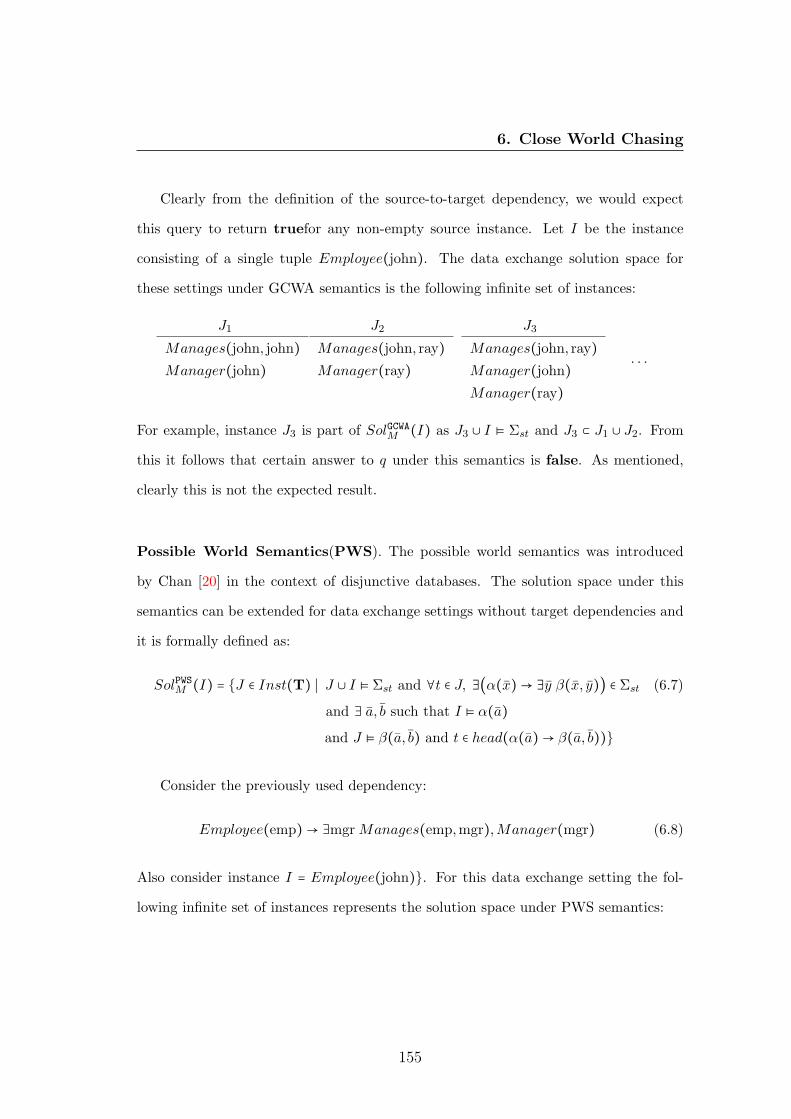
6. Close World Chasing
Clearly from the definition of the source-to-target dependency, we would expect
this query to return truefor any non-empty source instance. Let I be the instance
consisting of a single tuple Employee(john). The data exchange solution space for
these settings under GCWA semantics is the following infinite set of instances:
J1
Manages(john, john)Manager(john)
J2
Manages(john, ray)Manager(ray)
J3
Manages(john, ray)Manager(john)Manager(ray)
. . .
For example, instance J3 is part of SolGCWAM (I) as J3 ∪ I ⊧ Σst and J3 ⊂ J1 ∪ J2. From
this it follows that certain answer to q under this semantics is false. As mentioned,
clearly this is not the expected result.
Possible World Semantics(PWS). The possible world semantics was introduced
by Chan [20] in the context of disjunctive databases. The solution space under this
semantics can be extended for data exchange settings without target dependencies and
it is formally defined as:
SolPWSM (I) = {J ∈ Inst(T) ∣ J ∪ I ⊧ Σst and ∀t ∈ J, ∃(α(x) → ∃y β(x, y)) ∈ Σst (6.7)
and ∃ a, b such that I ⊧ α(a)
and J ⊧ β(a, b) and t ∈ head(α(a) → β(a, b))}
Consider the previously used dependency:
Employee(emp) → ∃mgr Manages(emp,mgr),Manager(mgr) (6.8)
Also consider instance I = Employee(john)}. For this data exchange setting the fol-
lowing infinite set of instances represents the solution space under PWS semantics:
155
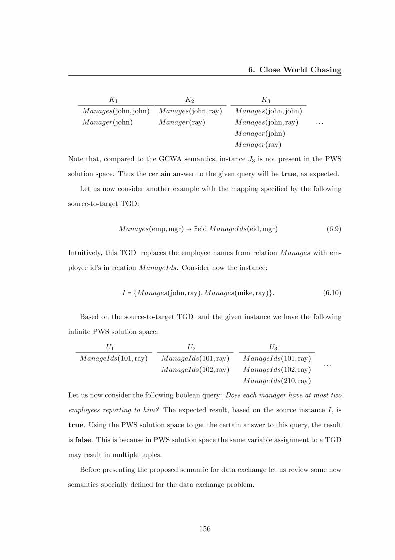
6. Close World Chasing
K1
Manages(john, john)Manager(john)
K2
Manages(john, ray)Manager(ray)
K3
Manages(john, john)Manages(john, ray)Manager(john)Manager(ray)
. . .
Note that, compared to the GCWA semantics, instance J3 is not present in the PWS
solution space. Thus the certain answer to the given query will be true, as expected.
Let us now consider another example with the mapping specified by the following
source-to-target TGD:
Manages(emp,mgr) → ∃eid ManageIds(eid,mgr) (6.9)
Intuitively, this TGD replaces the employee names from relation Manages with em-
ployee id’s in relation ManageIds. Consider now the instance:
I = {Manages(john, ray),Manages(mike, ray)}. (6.10)
Based on the source-to-target TGD and the given instance we have the following
infinite PWS solution space:
U1
ManageIds(101, ray)
U2
ManageIds(101, ray)ManageIds(102, ray)
U3
ManageIds(101, ray)ManageIds(102, ray)ManageIds(210, ray)
. . .
Let us now consider the following boolean query: Does each manager have at most two
employees reporting to him? The expected result, based on the source instance I, is
true. Using the PWS solution space to get the certain answer to this query, the result
is false. This is because in PWS solution space the same variable assignment to a TGD
may result in multiple tuples.
Before presenting the proposed semantic for data exchange let us review some new
semantics specially defined for the data exchange problem.
156

6. Close World Chasing
CWA-solutions. The CWA-solutions approach was first introduced by Libkin [54]
for mappings specified by a set of source-to-target TGD’s. This approach is based on
the intuition that any fact in the target instance should follow logically from the source
instance and the set of dependencies, and also that no two nulls in the target should be
gratuitously equated. This is formalized using a new notion called justification. These
justifications conveniently restrict the solutions to the universal ones, called closed world
solutions in [54], here denoted as SolCWASOLM (I). Hernich and Schweikardt [47] extended
Libkin’s justification based approach by allowing the mapping to be specified by target
TGD’s and they generalize the set SolCWASOLM (I). Their solution space has the peculiarity
that there are generalized instances J ∈ SolCWASOLM (I) such that repCWA(J)∪I /⊧ Σst∪Σt.
The certain answer to a target query q under the previously presented data exchange
settings is defined as:
⋂J∈Sol
CWASOLM (I)
⋂K∈repCWA(J),K∪I⊧Σ
q(K). (6.11)
Without going in too much detail, we need to mention that it is enough to materialize
the set of “maximal“ CWA-solutions in order to get certain answers to FO-queries.
Consider for example the data exchange mapping M specified by the following set of
TGD’s:
Σst ∶ Scholar(s) → Student(s) (6.12)
Scholar(s) → ∃m1,m2 Major(s,m1,m2) (6.13)
Σt ∶ Major(s,m,m) → StdOneMajor(s) (6.14)
Consider the source instance I = {Scholar(john)}. The unique maximal CWA-solution
is instance J = {Student(john),Major(john,M1,M2)}. Now, for the following query
q(x) → Student(x)∧¬StdOneMajor(x), one would expect the certain answer to return
the empty set, as it may be possible that student “john“ has only one major. On the
157

6. Close World Chasing
other hand, running the query against the maximal solution, the certain answer for this
query is “john“. Clearly not the expected result.
GCWA∗. We conclude this section with the latest closed world semantics, namely
GCWA∗, introduced by Hernich [45], as an improvement for some of the previously
described anomalies. In certain query answering, GCWA∗ semantics was also proved
to be closed under logical equivalence of mappings. The new semantics generalizes the
GCWA one by considering a ground instance part of the data exchange solution space
if the instance is the union of some minimal solutions. More formally, the solution
space under GCWA∗ can be described as the following set:
SolGCWA∗
M (I) = {J ∈ Inst(T)∣ J ∪ I ⊧ Σ, J = ⋃i∈[n]
Ki for some Ki ∈⊆min (M,I)} (6.15)
For this semantics, Hernich proved that when the mappings are specified by a special
class of TGD’s, called packed TGD’s, and if the core of the universal solution is given,
then one may compute the certain answer in polynomial time. In case the core of the
universal solution is not provided and the core-chase algorithm terminates, then one
may find the certain answer in NP time with a DP oracle ([28]).
Let us now see an example of certain answer under GCWA∗ semantics. Consider a
mapping M specified by the following two source-to-target TGD’s:
Manages(emp,mgr) → ∃eid ManageIds(eid,mgr) (6.16)
SelfManager(mgr,mgrid) → ManageIds(mgrid,mgr) (6.17)
Where the first dependency has the same meaning as the second example used for
PWS semantics, and the second dependency specifies that each manager with the id
(“mgrid“) from the relation SelfManager is his own manager under target relation
ManageIds. Let us now add to this mapping the source instance:
158

6. Close World Chasing
I = {Manages(john, ray),Manages(mike, ray), SelfManager(ray,411)}. (6.18)
Finally, consider the query: Does each manager manage exactly one employee? It
is easy to see that under natural semantics one may expect the certain answer to this
query to be false , as it may be that the employee id’s, assigned for each employee from
the Manages relation, are distinct. On the other hand, the set ⊆min (M,I contains
only the instance J = {ManageIds(ray,411)}. Thus, under the GCWA∗ semantics the
certain answer to the given query is true, which is clearly not the expected result. The
same unnatural behavior can be observed even in case the mapping is specified only by
the first dependency with the same source instance and the query: Do all the managers
manage at most 2 employees each? In this case, the certain answer will be false under
GCWA∗, because the solution space is infinite, whereas the expected natural result
should be true.
6.2 Constructible Models Semantics
In the previous section we saw a few closed world semantics and their unnatural be-
havior when getting the certain answers for some general queries. In this section (part
of these results were first presented in [38]) we propose a new closed world semantics
which, we argue, is a good candidate as a closed world semantics for data exchange,
even if there are a few drawbacks with it. One such drawback is that the constructible
models semantics are not closed under the mapping equivalence, as shown by the fol-
lowing example:
Example 36 Consider the following two sets of source-to-target mappings:Σ1 = {R(x, y) → T (x, y)}
Σ2 = {R(x, y) → T (x, y); R(x, y) → ∃z T (x, z)}
159

6. Close World Chasing
Clearly Σ1 is logically equivalent with Σ2, i.e. I ⊧ Σ1 iff I ⊧ Σ2 for any instance
I. On the other hand considering source instance I = {R(a, b)} under constructible
models semantics we have {{T (a, b)}} as the solution space under Σ1 and the infinite
set {{T (a, b)},{T (a, b), T (a, a)},{T (a, b), T (a, c)}, . . .} as the solution space under Σ2.
Here are some strong points attached to this new semantics:
1. natural certain/possible answers for most FO queries. At the end of this section
we will review all the previous examples and see that the certain answer obtained
under this new semantic is the expected one.
2. there exists a simple chase based procedure able to compute the target instance
that may be used to compute certain answers.
3. in case the chase procedure terminates, there exists a single instance, usually of
small size, that needs to be materialized on the target.
Let I be a ground instance and Σ a set of TGD’s. Consider a standard-chase step
on I with TGD ξ = α(x, y) → ∃z β(x, z) and trigger (ξ, h). Instead of adding the tuple
head(β(h(x), z)), where Z is a sequence of new fresh variables, we create a branch for
each sequence c of constants and add the ground tuple β(h(x), c) to I. Continuing
in this fashion, we will have a chase tree, instead of a chase sequence. Notably, all
nodes in the tree will be ground instances. The leaves of the chase tree form the set
of constructible models of I and Σ, denoted Σ(I). If the initial input to the chase is
a general instance (that may contain nulls) J , the constructible solutions of J with Σ
will be Σ(repCWA(J)) = ⋃I∈repCWA(J) Σ(I).
More formally, let Σ be a finite set of TGD’s. Then the set of variables occurring in
Σ is finite. Consequently, there is an enumeration, say v0, v1, . . . , vn, . . ., of all mappings
(i.e. valuations) from this set of variables to ΔC. We define
160
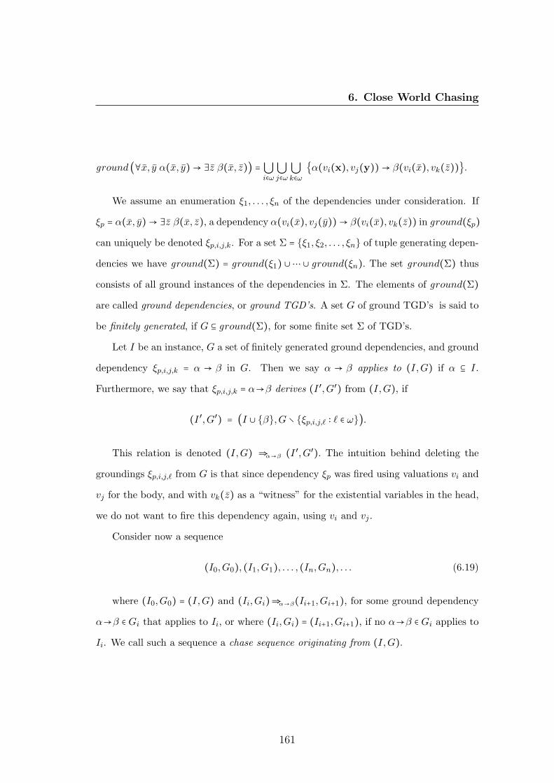
6. Close World Chasing
ground (∀x, y α(x, y) → ∃z β(x, z)) = ⋃i∈ω
⋃j∈ω
⋃k∈ω
{α(vi(x), vj(y)) → β(vi(x), vk(z))}.
We assume an enumeration ξ1, . . . , ξn of the dependencies under consideration. If
ξp = α(x, y) → ∃z β(x, z), a dependency α(vi(x), vj(y)) → β(vi(x), vk(z)) in ground(ξp)
can uniquely be denoted ξp,i,j,k. For a set Σ = {ξ1, ξ2, . . . , ξn} of tuple generating depen-
dencies we have ground(Σ) = ground(ξ1) ∪ ⋯ ∪ ground(ξn). The set ground(Σ) thus
consists of all ground instances of the dependencies in Σ. The elements of ground(Σ)
are called ground dependencies, or ground TGD’s. A set G of ground TGD’s is said to
be finitely generated, if G ⊆ ground(Σ), for some finite set Σ of TGD’s.
Let I be an instance, G a set of finitely generated ground dependencies, and ground
dependency ξp,i,j,k = α → β in G. Then we say α → β applies to (I,G) if α ⊆ I.
Furthermore, we say that ξp,i,j,k = α→β derives (I ′,G′) from (I,G), if
(I ′,G′) = (I ∪ {β},G ∖ {ξp,i,j,� ∶ ∈ ω}).
This relation is denoted (I,G) ⇒α→β (I ′,G′). The intuition behind deleting the
groundings ξp,i,j,� from G is that since dependency ξp was fired using valuations vi and
vj for the body, and with vk(z) as a “witness” for the existential variables in the head,
we do not want to fire this dependency again, using vi and vj .
Consider now a sequence
(I0,G0), (I1,G1), . . . , (In,Gn), . . . (6.19)
where (I0,G0) = (I,G) and (Ii,Gi)⇒α→β(Ii+1,Gi+1), for some ground dependency
α→β ∈ Gi that applies to Ii, or where (Ii,Gi) = (Ii+1,Gi+1), if no α→β ∈ Gi applies to
Ii. We call such a sequence a chase sequence originating from (I,G).
161

6. Close World Chasing
A chase sequence originating from (I,G) is said to be fair if for all ground de-
pendencies ξp,i,j,k ∈ G, for which there exists an n ∈ ω such that ξp,i,j,k applies to
(In,Gn). There also exists m, ∈ ω, m ≥ n such that (Im,Gm)⇒α→β(Im+1,Gm+1),
where α → β = ξp,i,j,�. Fairness means that all applicable dependencies are eventually
fired for some instantiation of the existential variables in the head. From now on, unless
stated otherwise, we consider all chase sequences to be fair.
It is obvious that Ii ⊆ Ii+1 and that Gi ⊇ Gi+1, for each i ∈ ω. We can therefore
define the limit of a chase sequence as
(⋃i∈ω
Ii,⋂i∈ω
Gi). (6.20)
The notation C(I,G) will stand for the set of the limits of all chase sequences
originating from (I,G).
We are now ready to define Σ(I), the set of all constructible models of I and Σ, as
Σ(I) = {J ∶ (J,G) ∈ C(I, ground(Σ)),G ⊆ ground(Σ)}. (6.21)
It is clear that the definition of Σ(I) does not depend on the particular enumeration
of the valuations of the variables in the dependencies in Σ. Note also that Σ(I) may
contain finite as well as infinite ground instances.
The following lemma derives directly from the definition of Σ(I):
Lemma 7 Σ(I) ⊆ Sat(Σ), where Sat(Σ) denotes the set of all instances I such that
I ⊧ Σ.
The definition of function Σ(I) is extended to a set of ground instances I point-wise
as follows:
Σ(I) = ⋃I∈I
Σ(I). (6.22)
162

6. Close World Chasing
The data exchange solution space under constructible models semantics can be
formalized as follows:
Definition 35 Let M = (S,T,Σst,Σt) be a data exchange mapping specified by a set
of TGD’s. Let I ∈ Inst(S) be a source instance. The solution space for M and I
under constructible models semantics is the following set of ground instances, where
Σ = Σst ∪Σt:
SolCMM(I) = {J ∈ Inst(T)∣ ∃K ∈ Σ(I) and J = K ∣T} (6.23)
Let us consider the following example that captures all the previous notions.
Example 37 Let Σ = {ξ}, where ξ is the sample TGD 6.8 used to present the PWS
semantic.
Manages(emp,mgr) → ∃eid ManageIds(eid,mgr) (6.24)
The grounding ground(ξ) is the following infinite set of ground dependencies:
ground(ξ) = {Manages(john, ray) → ManageIds(101, ray); (6.25)
Manages(john, ray) → ManageIds(102, ray);
Manages(john, ray) → ManageIds(103, ray); . . .
Manages(mike, ray) → ManageIds(101, ray);
Manages(mike, ray) → ManageIds(102, ray);
Manages(mike, ray) → ManageIds(103, ray); . . .
Manages(ann, ray) → ManageIds(101, ray);
Manages(ann, ray) → ManageIds(102, ray);
Manages(ann, ray) → ManageIds(103, ray); . . .
. . .
Manages(ray, john) → ManageIds(101, john); . . .
. . . }
163

6. Close World Chasing
As Σ = {ξ}, it follows that G = ground(ξ). Figure 6.1 represents the chase tree
corresponding to ground(Σ) and instance:
I = {Manages(john, ray),Manages(mike, ray)}. (6.26)
In figure 6.1 it can also be observed that, after applying to (I,G) the ground dependency
Manages(john, ray) → ManageIds(101, ray), we change the existing set of ground-
ings to G1 = G ∖ {Manages(john, ray) → ManageIds(*,*)}. That is G1 will not
contain any ground dependency with the body Manages(john, ray). Thus the tuple
Manages(john, ray) from I will not contribute to any other tuple in the limit instance.
This ensures that each tuple from the limit is “justified“ by different tuples in the in-
stance or by a different dependency. We may note that in this example, because the
dependency is a source-to-target TGD, the depth of the tree is 2. Thus there are finite
limits for each branch of the chase tree.
The solution space under constructible models semantics for the data exchange set-
tings specified in the previous example is given by the following infinite set of instances:
J1
ManageIds(101, ray)
J2
ManageIds(101, ray)ManageIds(102, ray)
J3
ManageIds(102, ray) . . .
Let us now reconsider the query: Do all managers have at most two employees each? for
which the certain answer under PWS semantics was false. Under constructible models
semantics the certain answer is, the expected one, true, as each branch in chase tree
from Figure 6.1 has depth 2 with the target instance containing at most two tuples.
In the remaining part of this section we will review each of the examples used for
the different closed words semantics presented in Section 6.1. First let us start with the
mapping M specified by the TGD 6.5 presented for both CWA and GCWA semantics.
164

6. Close World Chasing
Figure 6.1: Chase tree
165

6. Close World Chasing
Employee(emp) → ∃mgr Manages(emp,mgr),Manager(mgr) (6.27)
Consider also the same source instance I = Employee(john). In this case the solu-
tion space under constructible models semantics is the following infinite set of ground
instances:
K1
Manages(john, john)Manager(john)
K2
Manages(john, ray)Manager(ray)
K3
Manages(john,mike)Manager(mike)
. . .
Consider now the same query (6.6) presented for the CWA and GCWA semantics:
q ← ∀mgr Manager(mgr) → ∃emp Manages(emp,mgr) (6.28)
Under both semantics CWA and GCWA, the certain answer to this query was false.
Under our new semantic the certain answer to this query is, again the expected one,
true.
Under CWA-solution semantics we considered the mapping M specified by the
following source-to-target and target TGD’s :
Σst ∶ Scholar(s) → Student(s) (6.29)
Scholar(s) → ∃m1,m2 Major(s,m1,m2) (6.30)
Σt ∶ Major(s,m,m) → StdOneMajor(s) (6.31)
The solution space under constructible models semantics for M and source instance
I = {Scholar(john)} is the following infinite set of ground instances:
U1
Student(john)Major(john, c1, c2)
U2
Student(john)Major(john, c1, c3)
U3
Student(john)Major(john, c1, c1)StdOneMajor(john)
. . .
166
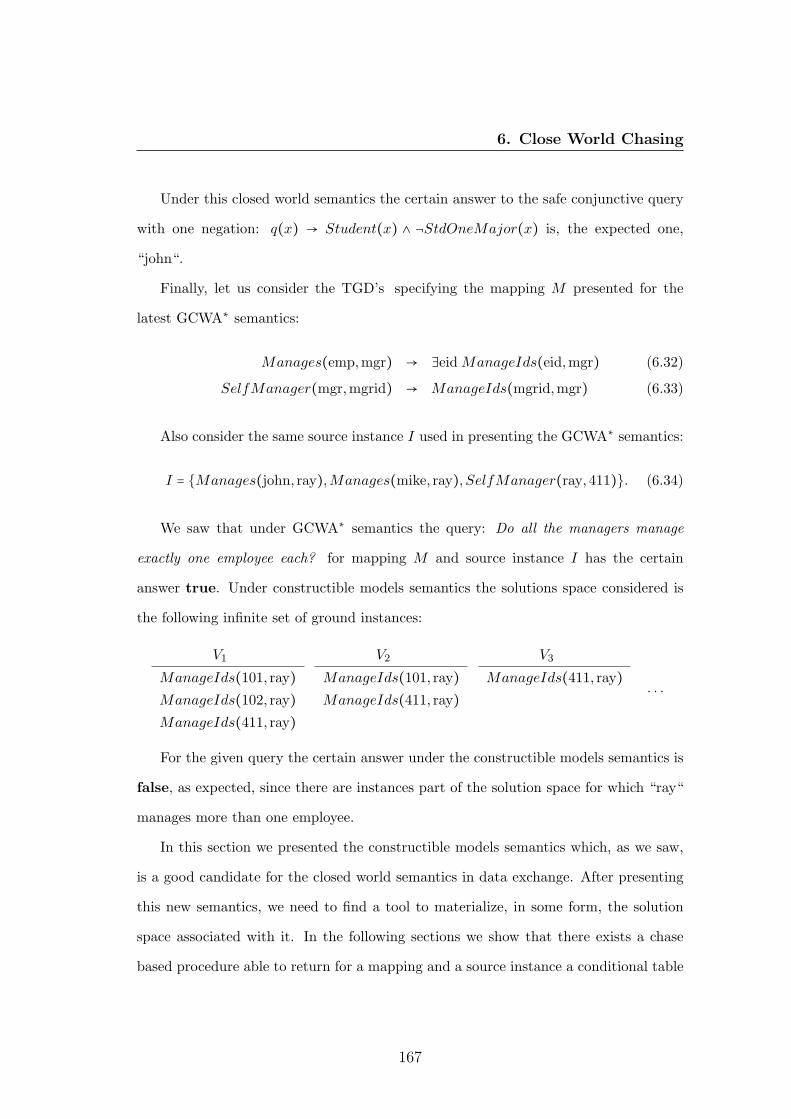
6. Close World Chasing
Under this closed world semantics the certain answer to the safe conjunctive query
with one negation: q(x) → Student(x) ∧ ¬StdOneMajor(x) is, the expected one,
“john“.
Finally, let us consider the TGD’s specifying the mapping M presented for the
latest GCWA∗ semantics:
Manages(emp,mgr) → ∃eid ManageIds(eid,mgr) (6.32)
SelfManager(mgr,mgrid) → ManageIds(mgrid,mgr) (6.33)
Also consider the same source instance I used in presenting the GCWA∗ semantics:
I = {Manages(john, ray),Manages(mike, ray), SelfManager(ray,411)}. (6.34)
We saw that under GCWA∗ semantics the query: Do all the managers manage
exactly one employee each? for mapping M and source instance I has the certain
answer true. Under constructible models semantics the solutions space considered is
the following infinite set of ground instances:
V1
ManageIds(101, ray)ManageIds(102, ray)ManageIds(411, ray)
V2
ManageIds(101, ray)ManageIds(411, ray)
V3
ManageIds(411, ray). . .
For the given query the certain answer under the constructible models semantics is
false, as expected, since there are instances part of the solution space for which “ray“
manages more than one employee.
In this section we presented the constructible models semantics which, as we saw,
is a good candidate for the closed world semantics in data exchange. After presenting
this new semantics, we need to find a tool to materialize, in some form, the solution
space associated with it. In the following sections we show that there exists a chase
based procedure able to return for a mapping and a source instance a conditional table
167

6. Close World Chasing
such that its representation is exactly the solution space under constructible models
semantics.
6.3 Conditional Tables and Unification Process
Before presenting the chase procedure able to create the solution space under con-
structible models semantics, we introduce now some new notions and review some
existing ones needed to introduce the chase procedure based on conditional tables. For
this, first we present the conditional tables in a way that clearly shows that they are
generalizations of general instances. We then introduce the concept of unification of
two instances which is needed as a technical tool for generalizing the standard-chase
algorithm to our conditional chase, introduced in Section 6.4. For the ease of notation,
in this section, we will refer by instance to a ground instance. This, we will refer as
tableau to the instance that may contain null values.
6.3.1 Conditional Tables
A conditional table (c-table) [49] is a pair (T,ϕ), where T is a tableau, and ϕ is a
mapping that associates a local condition ϕ(t) with each tuple t ∈ T . A (local) condition
is a Boolean formula built up from atoms of the form x = y, x ≠ y, x = a, x ≠ a, a = b
and a ≠ b for x, y ∈ ΔN and a, b ∈ ΔC. An atomic equality of the form a = a for a ∈ ΔC
represents the logical constant true and for two distinct constants a and b the equality
a = b represents false. We denote the logical implication between conditions ϕ and φ
by ϕ ⊧ φ and their logical equivalence by ϕ ≡ φ.
If ϕ(t) ≡ true, for all t ∈ T , the conditional table (T,ϕ) is sometimes denoted simply
with T .
A conditional table (T,ϕ) represents a set of possible worlds (ground instances).
168
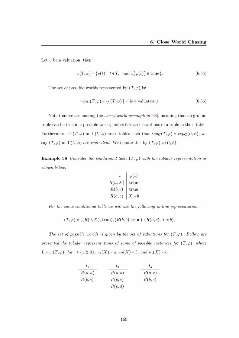
6. Close World Chasing
Let v be a valuation, then:
v(T,ϕ) = {v(t) ∣ t ∈ T, and v(ϕ(t)) ≡ true}. (6.35)
The set of possible worlds represented by (T,ϕ) is:
repC(T,ϕ) = {v(T,ϕ) ∣ v is a valuation}. (6.36)
Note that we are making the closed world assumption [68], meaning that no ground
tuple can be true in a possible world, unless it is an instantions of a tuple in the c-table.
Furthermore, if (T,ϕ) and (U,φ) are c-tables such that repC(T,ϕ) = repC(U,φ), we
say (T,ϕ) and (U,φ) are equivalent. We denote this by (T,ϕ) ≡ (U,φ).
Example 38 Consider the conditional table (T,ϕ) with the tabular representation as
shown below:
t ϕ(t)
R(a,X) true
R(b, c) true
R(a, c) X = b
For the same conditional table we will use the following in-line representation:
(T,ϕ) = {(R(a,X), true), (R(b, c), true), (R(a, c),X = b)}
The set of possible worlds is given by the set of valuations for (T,ϕ). Bellow are
presented the tabular representations of some of possible instances for (T,ϕ), where
Ii = vi(T,ϕ), for i ∈ {1,2,3}, v1(X) = a, v2(X) = b, and v3(X) = c.
I1
R(a, a)R(b, c)
I2
R(a, b)R(b, c)R(c, d)
I3
R(a, c)R(b, c)
169

6. Close World Chasing
When it comes to dependencies, a conditional table (T,ϕ) is said to satisfy a set
Σ of dependencies, if all possible worlds it represents satisfy Σ, that is, if we have
repC(T,ϕ) ⊆ Sat(Σ).
Example 39 Consider the conditional table (T,ϕ) from example 38 and the depen-
dencies Σ1 = {R(x, y),R(y, z) → R(x, z)} and Σ2 = {R(x, y) → ∃z R(y, z)}. Clearly we
have repC(T,ϕ) ⊆ Sat(Σ1). On the other hand, the same conditional table (T,ϕ) does
not satisfy Σ2 as, for example, in I1 we have tuple R(b, c) but there is no tuple in I1
that has c as value in the first column in relation R, thus I1 /⊧ Σ2.
The standard chase on instances is essentially a fixed point computation, where the
underlying partial order is that of set inclusion. The conditional chase will also be a
fixed point computation, so we will need a suitable partial order on conditional tables.
Let (T,ϕ) and (U,ψ) be c-tables, by (T,ϕ) ⊑ (U,φ) we mean that T ⊆ U and that, for
all valuations v, it is that v(T,ϕ) ⊆ v(U,φ).
If both (T,ϕ) ⊑ (U,φ) and (T,ϕ) ⊑ (U,φ), we write (T,ϕ) ≅ (U,φ) and say that
the c-tables are congruent. Obviously (T,ϕ) ≅ (U,φ) if and only if T = U and for all
valuations v, v(T,ϕ) = v(U,φ). Consider the following binary union operation between
conditional tables: (T,ϕ) ⊔ (U,φ) =def. (T ∪U,ϕ⊔φ), where
ϕ⊔φ (t) =
⎧⎪⎪⎪⎪⎪⎨⎪⎪⎪⎪⎪⎩
ϕ(t) ∨ φ(t) if t ∈ T ∩U,
ϕ(t) if t ∈ T ∖U,
φ(t) if t ∈ U ∖ T.
(6.37)
Thus ⊔ is a partial order on equivalence classes under ≅ of c-tables. Recall that two
conditional tables are equivalent if they represent the same set of possible worlds. The
following lemma states that congruence is stronger than equivalence.
Lemma 8 Let (T,ϕ) and (U,φ) be two conditional tables. If (T,ϕ) ≅ (U,φ), then
(T,ϕ) ≡ (U,φ). There are c-tables (T,ϕ) and (U,φ), such that (T,ϕ) ≡ (U,φ) and
(T,ϕ) /≅ (U,φ).
170

6. Close World Chasing
Proof: Let us suppose that (T,ϕ) ≅ (U,φ). From the definition of ≅ it follows that
T = U and for all valuations v and tuples t ∈ T if φ(t) ≡ true, then v(t) ∈ v(T,ϕ) and
inverse. Let v be a valuation, we will show that v(U,φ) = v(T,ϕ). Let t ∈ v(U,φ).
It follows that there exists a tuple tU ∈ U such that v(tU) = t and v(φ(tU)) = true.
From this it follows that t = v(tU) ∈ v(T,ϕ), thus v(U,φ) ⊆ v(T,ϕ). Similarly, it can be
proved that v(T,ϕ) ⊆ v(U,φ). For the second part of this lemma, consider conditional
tables (T,ϕ) = {(R(a, b), true)} and (U,φ) = {(R(a,X),X = b)}. It is easy to see that
(T,ϕ) ≡ (U,φ) but (T,ϕ) /⊑ (U,φ)∎
6.3.2 Unification of Tableaux
In order to extend the standard-chase procedure to conditional tables, in this section
we introduce first the notions of unifiers and most general unifiers for pairs of tableaux.
For this, let us first extend the notion of retraction (as defined in Section 2.1) to the
notion of D-retraction, for a set of constants D.
Definition 36 Let T be a tableau and let D be a finite set of constants. A D-retraction
for T is a mapping h ∶ dom(T ) → dom(T ) ∪D, identity on ΔC ∪ dom(h(T )).
Note that if D = ∅, then a D-retraction for T is a retraction for T . From now on
we will refer to a ∅-retraction simply as retraction.
Example 40 Let T = {R(a,X),R(a, Y ),R(a, b)} and D = {c, d}, then the mappings
h1 = {X/c}, h2 = {X/a, Y /a} are D-retractions for T . On the other hand, the mapping
h3 = {X/Y,Y /a} is not a D-retraction because h3 maps X to Y and it is not identity
on Y .
We shall also need the concept of an h-core of an instance, for a retraction h.
171

6. Close World Chasing
Definition 37 Let T be a tableau, D a set of constants, and h a D-retraction for T .
Then we say that T is an h- core, if there is no T ′ ⊊ T , such that h(T ′) = h(T ).
It is easy to see that a tableau T is a core if and only if T is an h-core for all
retractions h on T .
Example 41 Consider T = {R(a,X),R(a, b)} and retraction h = {X/b}. It is easy to
see that T is not an h-core because for T ′ = {R(a, b)} we have T ′ ⊊ T and h(T ′) = h(T ).
On the other hand, retraction h′ = {X/c} is an h′-core. Clearly tableau T is not a core.
Recall that for a tableau T by ΔC(dom(T )) we denote the set of all constants in T .
Definition 38 Let T and U be two tableaux. A unifier for tableaux T and U , if it
exists, is a pair (θ1, θ2), where θ1 is a homomorphism from the set dom(T ) to the
set dom(U) ∪ ΔC(dom(T )) and θ2 is a ΔC(dom(T ))-retraction for U , such that the
following holds θ1(T ) = θ2(U).
Note the asymmetrical role of T and U : a unifier for (T,U) is not necessarily a
unifier for (U,T ).
Example 42 Consider tableaux T = {R(a,X1,X1,X2)} and U = {R(Y1, b, Y2, Y3)}.
The pair (θ1, θ2), where θ1 = {X1/b,X2/b} and θ2 = {Y1/a, Y2/b, Y3/b} is a unifier for
T and U as θ1(T ) = θ2(U) = {R(a, b, b, b)}. It can be noticed that (θ1, θ2) is not
the unique unifier for T and U . For example (θ′1, θ′2), where θ′1 = {X1/b,X2/Y3} and
θ′2 = {Y1/a, Y2/b}, is also a unifier for T and U .
Definition 39 A unifier (θ1, θ2) for tableaux T and U is more general than a unifier
(γ1, γ2), if there is a mapping f on dom(U), f ∉ Id, identity on constants, such that
γ1 = f ○ θ1 and γ2 = f ○ θ2.
172

6. Close World Chasing
Clearly this defines a partial preorder on unifiers and a partial order on equivalence
classes of isomorphic unifiers. Two unifiers (θ1, θ2) and (γ1, γ2) of (T,U) are considered
isomorphic if θ1(T ) is isomorphic with γ1(T ).
Definition 40 A unifier (θ1, θ2) is a most general unifier (mgu) for tableaux T and
U , if all unifiers (γ1, γ2) of T and U that are more general than (θ1, θ2) actually are
isomorphic with (θ1, θ2). We denote by mgu(T,U) the set of (representatives of the)
equivalence classes of all mgu’s of T and U .
Example 43 In Example 42 unifier (θ′1, θ′2) is a more general unifier than (θ1, θ2) and
it is also an mgu. Let us consider another example over instances T = {R(X,Y ),R(Y,Z)}
and U = {R(a, V ),R(W,b)}. In this case, the only mgu of T and U is given by the
equivalence class of unifier ({X/a, Y /W,Z/b},{V /W}).
It is well known that, if two atoms are unifiable, then there exists a most general
unifier that is unique up to isomorphism. But, when unifying two tableaux, there
might be several non-isomorphic mgu’s. For example, let us consider the following
tableaux T = {R(X,Y ),R(Y,Z)} and U = {R(a, V ),R(b,W )}. Then (θ1, θ2), with
θ1 = {X/a, Y /b, Z/W} and θ2 = {V /b}, is an mgu for T and U . On the other hand, the
unifier (γ1, γ2), with γ1 = {X/b, Y /a,Z/V } and γ2 = {W /a}, is also an mgu for T and
U . It is easy to see that (γ1, γ2) and (θ1, θ2) are not isomorphic.
The following step is to find an upper bound for the complexity of the membership
problem for the set mgu(T,U). The next lemma follows directly from Definition 37.
Lemma 9 Let T and U be two tableaux and (θ1, θ2) a most general unifier for T and
U . If U is θ2-core, then ∣U ∣ ≤ ∣T ∣.
173

6. Close World Chasing
Proof: Obviously, if tableau U is a θ2-core, then ∣U ∣ = ∣θ2(U)∣, on the contrary, we
would have instance U ′ = θ2(U) such that U ′ ⊊ U and θ2(U ′) = θ2(U) (note that this
does not work if θ2 would be an endomorphism and not a retraction see Example 40).
On the other hand, we have that θ1(T ) = θ2(U), thus ∣T ∣ ≥ ∣U ∣∎
From this we now have:
Proposition 18 Let ∣U ∣ ≤ ∣T ∣ = c. Then the set mgu(T,U) can be computed in time
O((2c)2cc2).
Proof: Giving a pair of mapping (θ1, θ2), we can check if (θ1, θ2) is a unifier for T and
U in O(c) time. Given a unifier (θ1, θ2), we can check if (θ1, θ2) is an mgu in time
O(c2) using the following algorithm:
1 for X/c ∈ θ2
2 do
3 θ′2 ← θ2 ∖ {X/c}4 if exists θ′1 such that (θ′1, θ
′2) is a unifier for T and U
5 then return false
6 else return true
The testing at Step 4 can be done in time O(c), thus the algorithm runs in time O(c2).
The number of mappings from U to dom(U) ∪ const(T ) is bounded by (2c)c; similarly
the number of mappings from T to dom(U) ∪ const(T ) is bounded by (2c)c. Thus we
need to check with the previous algorithm (2c)2c unifiers each such checking running
in time O(c2). That is, the time needed to find the set mgu(T,U) is O((2c)2cc2)∎
6.3.3 The Core of Conditional Tables
Contrary to the standard-chase step, the conditional-chase one is more sophisticated.
For this reason, before presenting the conditional-chase algorithm, we need to introduce
174

6. Close World Chasing
a new function on conditional tables called the conditional core (or simply core). Given
a relation name R, we denote by R(X) a tuple over R, where X ∈ (ΔN ∪ΔC)arity(R).
Definition 41 Let R(X) and R(Y ) be two tuples over R. We say that θ is a tuple
unifier (or simply unifier) for R(X) and R(Y ), if θ(R(X)) = θ(R(Y )) and θ is a
mapping from set dom({R(X)})∪dom({R(Y )}), identity on ΔC with values in the set
(ΔN ∖ΔN({R(X),R(Y )})) ∪ΔC.
Note that it may be that there is no unifier between two tuples. Also, it can be
observed that the unifier is symmetric. That is, if θ is unifier for R(X) and R(Y ), then
θ is also a unifier for R(Y ) and R(X). We say that two tuples are unifiable if there
exists a unifier for those tuples. Also, note that the unifier assigns new null values, thus
the unifier does not reuse any nulls from the unified tuples.
Example 44 Consider tuples t1 ∶ R(a,X1, c) and t2 ∶ R(X2,X3, c). The mappings
θ1 = {X1/d,X2/a,X3/d}, θ2 = {X1/X,X2/a,X3/X} are unifiers for t1 and t2, where
X is a new null value. On the other hand, the mapping θ3 = {X1/X3,X2/a} is not a
unifier even if θ3(t1) = θ2(t2), because it maps null X1 to existing null X3.
Similarly to the unifiers between instances, we have the notion of more general
unifier for tuples.
Definition 42 Let also θ1, θ2 be two unifiers for tuples t1 and t2. We say that θ1 is
a more general unifier than θ2 if there exists a non-isomorphic mapping f ∉ Id, that is
identity on constants, such that θ2 = f ○ θ1.
Returning to Example 44, θ2 is a more general unifier than θ1 for tuples t1 and t2.
Definition 43 A unifier θ is said to be a most general unifier for tuples t1 and t2 if
there does not exist unifier θ′ such that θ′ is more general than θ.
175

6. Close World Chasing
Clearly any two most general unifiers for two tuples t1 and t2 are isomorphic. By
mgu(t1, t2) we denote a representative unifier from the equivalence class of most general
unifiers for t1 and t2. For a unifier θ we shall use the abbreviation:
F (θ) =def ( ⋀X,Y ∈ΔN, θ(X)=θ(Y )
X = Y ) ∧ ( ⋀X∈ΔN, a∈ΔC, θ(X)=a
X = a) (6.38)
Example 45 Returning to the unifiers mentioned in Example 44, F(θ1) represents the
formula: X1 = d ∧X2 = a ∧X3 = d. and F(θ2) represents: X1 = X3 ∧X2 = a.
Definition 44 A conditional table (T,ϕ) is said to be a conditional core if for any
valuation v and for any two distinct tuples t1, t2 ∈ T it cannot be that v(t1) = v(t2) and
v(ϕ(t1)) ≡ v(ϕ(t2)) = true.
Example 46 Consider the following conditional table:
(T,ϕ)t ϕ(t)
R(a,X1, c) X5 = a
R(a, b,X2) X6 = b
R(X3,X4, c) X7 = c
R(a, b, c) X8 = d
For valuation v = {X1/b,X2/c,X3/a,X4/b,X5/a,X6/b,X7/d,X8/d} we have for all
tuples t ∈ T , v(t) = R(a, b, c) and v(ϕ(t)) ≡ true. Thus (T,ϕ) is not a conditional core.
Lemma 10 Given a conditional table (T,ϕ) such that ϕ(t) ≡ true, for all t ∈ T , then
testing if (T,ϕ) is a conditional core can be done in time O(n2)
Proof: This testing comes up to checking if there are two unifiable tuples in T∎
The previous lemma considered the local conditions tautologies. However, for ar-
bitrary boolean formula over equalities and inequalities, the problem becomes coNP-
complete.
176

6. Close World Chasing
Even if the complexity of checking if a conditional table is a conditional core is
coNP-complete in general, there exists a polynomial time algorithm that computes a
core for a conditional table, assuming that there exists a total order between the tuples
in the conditional table. Considering this, we denote the order relation between tuples
by the symbol “⋖“. In our conditional-chase algorithm, the order considered will be
the one in which the tuples are generated at each step. This is why in the following
algorithm we will traverse the tuples in descending order.
CORE-COMP((T,ϕ)
1 (U,φ) ← (T,ϕ), such that U = {t1, . . . , t∣T ∣} and tj ⋖ ti, for 1 ≤ i < j ≤ ∣T ∣.2 for i← 1 to ∣T ∣ − 13 do4 for j ← i + 1 to ∣T ∣5 do6 if ti is unifiable with tj7 then8 θ ←mgu(ti, tj)9 φ(ti) ← φ(ti) ∧ ¬� (θ)
10 φ(tj) ← φ(tj) ∨ (φ(ti) ∧�(θ))11 return (U,φ)
Figure 6.2: The Conditional Table Core Computation
Figure 6.2 presents the CORE-COMP (T,ϕ) algorithm which computes the core
of a given conditional table (T,ϕ) with the tuples ordered by ⋖. It is easy to observe
that this algorithm runs in time O(n2), where n = ∣T ∣. As the algorithm is deterministic
and terminates for all input conditional tables by CORE-COMP (T,ϕ), we will also
denote the conditional table returned by the algorithm. The following theorem states
the main result of this section:
Theorem 54 Let (T,ϕ) be a conditional table with a total order ⋖ on the tuples in T ,
177

6. Close World Chasing
then CORE-COMP (T,ϕ) is a conditional core and CORE-COMP (T,ϕ) ≅ (T,ϕ).
Proof: First we will prove that CORE-COMP (T,ϕ) is a conditional core. Let us
denote (U,φ) = CORE-COMP (T,ϕ). Towards a contradiction let us assume that
(U,φ) is not a conditional core. Thus, there exist a valuation v and the tuples t1, t2 ∈ U ,
such that v(φ(t1)) ≡ v(φ(t2)) ≡ true and v(t1) = v(t2). Wlog. We may assume that
t2 ⋖ t1, if not we interchange the notation of the two tuples. Because v(t1) = v(t2), it
follows that v is a unifier for t1 and t2, thus there exists θ = mgu(t1, t2). On the other
hand, because t2 ⋖ t1, it follows, from the description of the algorithm, that φ(t1) is a
formula of the form μ∧¬F(θ). Where μ is an expression, because t1 is unified with t2
only after all the unification between t1 and t (line 6 of the algorithm) took place, for
all t such that t1 ⋖ t. On the other hand, because θ is a more general unifier than v, it
follows that F(v) ⊧ F(θ), v(φ(t1)) = v(μ ∧ ¬F (θ)), thus v(φ(t1)) = v(μ) ∧ ¬v(F(θ)).
But we have that v(F(θ)) ≡ true following v(φ(t1)) = false contradicting with the
initial assumption that v(φ(t1)) ≡ true.
Before continuing the proof, let us introduce a few notations, where t is a tuple and
v a valuation:
• Let parent(t) be the ordered sequence (t1, . . . , tn) such that tj ⋖ ti, for all integers
1 ≤ i < j ≤ n, ti ⋖ t (note that algorithm uses the descending order) and the tuples
ti and t are unifiable, for all i ∈ [n]. We denote by parentv(t) the subsequence of
sequence parent(t) such that, for any tuple t′ ∈ parentv(t), we have v(t′) = v(t).
• Let child(t) be the ordered sequence (t1, . . . , tn) such that tj ⋖ ti, for 1 ≤ i < j ≤ n,
t⋖ ti and the tuples t and ti are unifiable, for i ∈ [n]. We then denote by childv(t)the subsequence of child(t) such that, for any tuple t′ ∈ childv(t), we then have
v(t′) = v(t).
• It is clear that for any t ∈ U , φ(t) is a formula of the form:φ(t) = ((ϕ(t) ∨ μ1 ∨ . . . ∨ μn) ∧ γ1 ∧ . . . ∧ γm) (6.39)
where n = ∣parent(t)∣ and m = ∣child(t)∣. Each disjunct μi, i ∈ [n] was obtained
178

6. Close World Chasing
by unifying tuples ti ∈ parent(t) and t on line 10 of the algorithm. And each
conjunct γj , j ∈ [m] was obtained by unifying tuples t and tj ∈ child(t) on line 9
of the algorithm.
• For each t ∈ U , we denote by φ∗(t) the conjunct: (ϕ(t) ∨ μ1 ∨ . . . ∨ μn) from the
formula φ(t) specified in 6.39.
It can be easily observed that ∣parentv(t)∣ > ∣parentv(t′)∣, for any t′ ∈ parentv(t).
Also ∣childv(t)∣ > ∣childv(t′)∣ for any t′ ∈ childv(t). Note that ∣parent(t)∣ > ∣parent(t′)∣
for any t′ ∈ parent(t) it does not always hold (the same for child sequence).
Returning to our proof, we need to show that (U,φ) ≅ (T,ϕ). Note that the
algorithm CORE-COMP does not add or eliminate tuples, thus U = T . Let us first
show that (U,φ) ⊑ (T,ϕ). For this let v be a valuation and t ∈ U . We need to prove
that if v(φ(t)) ≡ true then v(t) ∈ v(T,ϕ).
First we will prove that, by induction on the size of the set parentv(t) ∪ {t}, if
v(φ∗(t)) ≡ true, then there exists t′ ∈ (parentv(t) ∪ {t}) such that v(ϕ(t′)) ≡ true.
For the base case, let us suppose ∣parentv(t)∣ = 0 and v(φ∗(t)) ≡ true, where φ(t) is
of the form 6.39. Because ∣parentv(t)∣ = 0, it follows that there is no t′ ∈ parent(t) such
that v(t′) = v(t). On the other hand, because each disjunct μi, i ∈ [n] was obtained on
line 10 of the algorithm by unifying ti ∈ parent(t) to t using mgu θi, it follows that μi is
of the form λi ∧F(θi). But this means that v(F(θi)) ≡ false, because θi is the mgu for
ti, t and v is not a unifier for ti, t. Following that v(μi) ≡ false for all i ∈ [n], because
v(φ∗(t)) ≡ true, it follows that it needs to be that v(ϕ(t)) ≡ true. This proves the
base case.
For the induction step, we assume that, if for a tuple t we have ∣parentv(t)∣ = k and
v(φ∗(t)) ≡ true, then there exists tuple t′ ∈ (parentv(t)∪{t}) such that v(ϕ(t′)) ≡ true.
Let us now consider ∣parentv(t)∣ = k + 1 and v(φ∗(t)) ≡ true. If v(ϕ(t)) ≡ true, the
induction is proved. Let us suppose that v(ϕ(t)) ≡ false, thus there exists i ∈ [n] such
179

6. Close World Chasing
that v(μi) ≡ true (see formula 6.39). Where condition μi was added in step 10 of the
algorithm due to tuple ti ∈ parent(t). From the construction of the disjunct μi, we
have μi = λi ∧ F(θ), where λi = φ∗(ti) ∧ ρ1 ∧ . . . ∧ ρh. From the assumption we have
v(μi) ≡ true, thus v(F(θ)) ≡ true and v(λi) ≡ true following that v(φ∗(ti)) ≡ true.
On the other hand, from v(F(θ)) ≡ true it follows that v(t) = v(ti), thus ti ∈ parentv(t).
Meaning that ∣parentv(ti)∣ < ∣parentv(t)∣ = k + 1 and having also v(φ∗(ti)) ≡ true.
From the induction steps it follows that there exists a t′ ∈ (parentv(ti)∪{ti}) such that
v(ϕ(t′)) ≡ true. This concludes the proof that if v(φ∗(t)) ≡ true, then there exists
t′ ∈ (parentv(t) ∪ {t}) such that v(ϕ(t′)) ≡ true. But from the main assumption we
know that v(φ(t)) ≡ true, thus v(φ∗(t)) ≡ true. From the previous inductive proof it
follows that there exists t′ ∈ parentv(t) such that v(ϕ(t′)) ≡ true. From the definition
of parentv(t) sequence it follows that v(t′) = v(t), thus v(t) ∈ v(T,ϕ). By this we
showed that (U,φ) ⊑ (T,ϕ).
It remains to be proved that (T,ϕ) ⊑ (U,φ). Let us consider v a valuation and t a
tuple in T such that v(ϕ(t)) ≡ true. We need to show that v(t) ∈ v(U,φ).
Similarly to the previous proof, first we will demonstrate by induction on the size
of childv(t) ∪ {t} that if φ∗(t) ≡ true, then there exists t′ ∈ (childv(t) ∪ {t}) such that
v(φ(t′)) ≡ true. For the induction base case, let us suppose that ∣childv(t)∣ = 0 and
v(φ∗(t)) ≡ true. For the ease of reading we rewrite below the general format of φ(t):
φ(t) = ((ϕ(t) ∨ μ1 ∨ . . . ∨ μn) ∧ γ1 ∧ . . . ∧ γm) (6.40)
The assumption is v(φ∗(t)) ≡ true, this means that either v(φ(t)) ≡ true or there
exists a positive integer j ∈ [m] such that v(γj) ≡ false. Towards a contradiction, let
us suppose that there exists positive integer i ∈ [m] such that v(γj) ≡ false. From the
description of the formula 6.40 we know that each γj , j ∈ [m] is generated on line 9 of
the algorithm by unifying tuples t, tj using an mgu θj . Thus γj is of the form ¬F(θj).
180

6. Close World Chasing
Because v(γi) ≡ false, it follows that v(F(θj)) ≡ true, but because θj is an mgu for t,
tj , it follows that v(t) = v(tj), contradicting that ∣childv(t)∣ = 0. Thus it must be that
v(φ(t)) ≡ true, proving the base case.
For the induction step, let us suppose that for any tuple t if ∣childv(t)∣ = k and
v(φ∗(t)) ≡ true, then there tuple t′ ∈ (childv(t) ∪ {t}) such that v(φ(t′)) ≡ true. Let
us consider tuple t such that ∣childv(t)∣ = k+1 and v(φ∗(t)) ≡ true. If v(φ(t′)) ≡ true,
then the induction step is proved. Let us consider that we have v(φ(t′)) ≡ false, thus
from formula 6.40 it follows that there exists a smallest positive integer j ∈ [m] such that
v(γj) ≡ false and for all h ∈ [j] we have v(γh) ≡ true. As shown in the induction basic
case, γj is of the form ¬F (tj), where θj is the mgu between tuples t and tj ∈ child(t).
Because v(γi) ≡ false, then v(F(θj)) ≡ true. On the other hand, we have from line 10
of the algorithm that φ∗(tj) is a disjunctive formula that contains the following disjunct
λj = (φ∗(t) ∧ γ1 ∧ . . . ∧ γj−1 ∧ F(θj)). From the way j was chosen, it follows that, for
all h ∈ [j], we have that v(γh) ≡ true. We also have, from the induction assumption,
that v(φ∗(t)) ≡ true and we already showed that v(F(θj)) ≡ true. Therefore, we have
that v(λi) ≡ true. Because λj is a disjunct in φ∗(tj), it follows that v(φ∗(tj)) ≡ true.
Also we know that v(F(θj)) ≡ true, where θj is the mgu for tuples t, tj . It follows that
v(tj) = v(t) meaning that tj ∈ childv(t), thus ∣childv(tj)∣ < ∣childv(t)∣ = k + 1. Adding
that v(φ∗(tj)) ≡ true from the inductive assumption, it follows that there exists a
t′ ∈ (childv(tj) ∪ {tj}) such that v(φ(t′)) ≡ true. This concludes the inductive proof.
Now let t be a tuple from T such that v(ϕ(t)) ≡ true. As φ(t) is a disjunctive
formula containing the disjunct ϕ(t), it follows that v(φ∗(t)) ≡ true. From the previous
inductive proof, it follows that there exists a tuple t′ ∈ (childv(t)∪{t}) with the property
that v(φ(t′)) ≡ true. But because v(t′) = v(t), it follows that v(t) ∈ (U,φ), proving
that (T,ϕ) ⊑ (U,φ). From this and the previous result, it follows that (T,ϕ) ≅ (U,φ)∎
Example 47 Let us now exemplify some of the algorithm steps by considering the
181
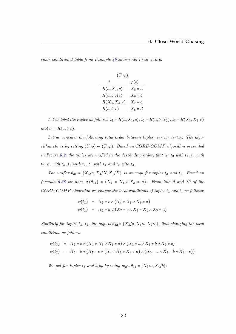
6. Close World Chasing
same conditional table from Example 46 shown not to be a core:
(T,ϕ)t ϕ(t)
R(a,X1, c) X5 = a
R(a, b,X2) X6 = b
R(X3,X4, c) X7 = c
R(a, b, c) X8 = d
Let us label the tuples as follows: t1 = R(a,X1, c), t2 = R(a, b,X2), t3 = R(X3,X4, c)
and t4 = R(a, b, c).
Let us consider the following total order between tuples: t4 ⋖ t2 ⋖ t1 ⋖ t3. The algo-
rithm starts by setting (U,φ) ← (T,ϕ). Based on CORE-COMP algorithm presented
in Figure 6.2, the tuples are unified in the descending order, that is: t3 with t1, t3 with
t2, t3 with t4, t1 with t2, t1 with t4 and t2 with t4.
The unifier θ31 = {X3/a,X4/X,X1/X} is an mgu for tuples t3 and t1. Based on
formula 6.38 we have F(θ31) = (X4 = X1 ∧ X3 = a). From line 9 and 10 of the
CORE-COMP algorithm we change the local conditions of tuples t3 and t1 as follows:
φ(t3) = X7 = c ∧ (X4 ≠ X1 ∨X3 ≠ a)
φ(t1) = X5 = a ∨ (X7 = c ∧X4 = X1 ∧X3 = a)
Similarly for tuples t3, t2, the mgu is θ32 = {X3/a,X4/b,X2/c}, thus changing the local
conditions as follows:
φ(t3) = X7 = c ∧ (X4 ≠ X1 ∨X3 ≠ a) ∧ (X3 ≠ a ∨X4 ≠ b ∨X2 ≠ c)
φ(t2) = X6 = b ∨ (X7 = c ∧ (X4 ≠ X1 ∨X3 ≠ a) ∧ (X3 = a ∧X4 = b ∧X2 = c))
We get for tuples t3 and t4by by using mgu θ34 = {X3/a,X4/b}:
182

6. Close World Chasing
φ(t3) = X7 = c ∧ (X4 ≠ X1 ∨X3 ≠ a) ∧ (X3 ≠ a ∨X4 ≠ b ∨X2 ≠ c)
∧(X3 ≠ a ∨X4 ≠ b)
φ(t4) = X8 = d ∨ (X7 = c ∧ (X4 ≠ X1 ∨X3 ≠ a) ∧ (X3 ≠ a ∨X4 ≠ b ∨X2 ≠ c)
∧(X3 = a ∧X4 = b))
The unifier θ12 = {X1/b,X2/c} is an mgu for t1 and t2, thus we have:
φ(t1) = (X5 = a ∨ (X7 = c ∧X4 = X1 ∧X3 = a)) ∧ (X1 ≠ b ∨X2 ≠ c)
φ(t2) = X6 = b ∨ (X7 = c ∧ (X4 ≠ X1 ∨X3 ≠ a) ∧ (X3 = a ∧X4 = b ∧X2 = c))
∨((X5 = a ∨ (X7 = c ∧X4 = X1 ∧X3 = a)) ∧ (X1 = b ∧X2 = c))
We have mgu θ14 = {X1/b} for tuples t1 and t4:
φ(t1) = (X5 = a ∨ (X7 = c ∧X4 = X1 ∧X3 = a)) ∧ (X1 ≠ b ∨X2 ≠ c) ∧ (X1 ≠ b)
φ(t4) = X8 = d ∨ (X7 = c ∧ (X4 ≠ X1 ∨X3 ≠ a) ∧ (X3 ≠ a ∨X4 ≠ b ∨X2 ≠ c)
∧(X3 = a ∧X4 = b))
∨((X5 = a ∨ (X7 = c ∧X4 = X1 ∧X3 = a)) ∧ (X1 ≠ b ∨X2 ≠ c) ∧ (X1 = b))
Finally, the unifier θ24 = {X2/c} is the mgu for t2, t4 changing their local conditions
to:
φ(t2) = (X6 = b ∨ (X7 = c ∧ (X4 ≠ X1 ∨X3 ≠ a) ∧ (X3 = a ∧X4 = b ∧X2 = c))
∨((X5 = a ∨ (X7 = c ∧X4 = X1 ∧X3 = a)) ∧ (X1 = b ∧X2 = c))) ∧ (X2 ≠ c)
φ(t4) = X8 = d ∨ (X7 = c ∧ (X4 ≠ X1 ∨X3 ≠ a) ∧ (X3 ≠ a ∨X4 ≠ b ∨X2 ≠ c)
∧(X3 = a ∧X4 = b))
∨((X5 = a ∨ (X7 = c ∧X4 = X1 ∧X3 = a)) ∧ (X1 ≠ b ∨X2 ≠ c) ∧ (X1 = b))
∨((X6 = b ∨ (X7 = c ∧ (X4 ≠ X1 ∨X3 ≠ a) ∧ (X3 = a ∧X4 = b ∧X2 = c))
∨((X5 = a ∨ (X7 = c ∧X4 = X1 ∧X3 = a)) ∧ (X1 = b ∧X2 = c))) ∧ (X2 = c))
Putting all together, the conditional table (U,φ) returned by the CORE-COMP
algorithm has the same tuples as (T,ϕ) with the following local conditions:
183

6. Close World Chasing
φ(t1) = (X5 = a ∨ (X7 = c ∧X4 = X1 ∧X3 = a)) ∧ (X1 ≠ b ∨X2 ≠ c) ∧ (X1 ≠ b)
φ(t2) = (X6 = b ∨ (X7 = c ∧ (X4 ≠ X1 ∨X3 ≠ a) ∧ (X3 = a ∧X4 = b ∧X2 = c))
∨((X5 = a ∨ (X7 = c ∧X4 = X1 ∧X3 = a)) ∧ (X1 = b ∧X2 = c))) ∧ (X2 ≠ c)
φ(t3) = X7 = c ∧ (X4 ≠ X1 ∨X3 ≠ a) ∧ (X3 ≠ a ∨X4 ≠ b ∨X2 ≠ c)
∧(X3 ≠ a ∨X4 ≠ b)
φ(t4) = X8 = d ∨ (X7 = c ∧ (X4 ≠ X1 ∨X3 ≠ a) ∧ (X3 ≠ a ∨X4 ≠ b ∨X2 ≠ c)
∧(X3 = a ∧X4 = b))
∨((X5 = a ∨ (X7 = c ∧X4 = X1 ∧X3 = a)) ∧ (X1 ≠ b ∨X2 ≠ c) ∧ (X1 = b))
∨((X6 = b ∨ (X7 = c ∧ (X4 ≠ X1 ∨X3 ≠ a) ∧ (X3 = a ∧X4 = b ∧X2 = c))
∨((X5 = a ∨ (X7 = c ∧X4 = X1 ∧X3 = a)) ∧ (X1 = b ∧X2 = c))) ∧ (X2 = c))
Consider v1 = {X1/d,X2/c,X3/a,X4/d,X5/a,X6/b,X7/c,X8/d} a valuation for (U,φ).
In this case we have v1(φ1) ≡ true, v1(φ2) ≡ false, v1(φ3) ≡ false and v1(φ4) ≡ true,
giving v1(U,φ) = {R(a, d, c),R(a, b, c)} equal to v1(T,ϕ). Note that v1(ϕ(t4)) ≡ false
and v1φ(t4)) ≡ true.
We conclude this section with another example of a conditional table that has
isomorphic tuples:
Example 48 Let (T,ϕ) be the following conditional table:
(T,ϕ)t ϕ(t)
R(a,X1) true
R(a,X2) true
R(a,X3) true
The CORE − COMP algorithm with this input will return the conditional table
(U,φ) with the following tabular specification:
184
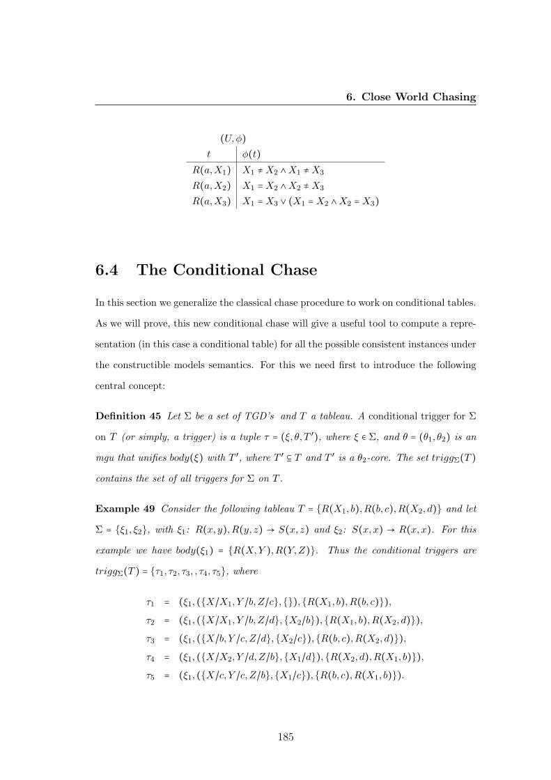
6. Close World Chasing
(U,φ)t φ(t)
R(a,X1) X1 ≠ X2 ∧X1 ≠ X3
R(a,X2) X1 = X2 ∧X2 ≠ X3
R(a,X3) X1 = X3 ∨ (X1 = X2 ∧X2 = X3)
6.4 The Conditional Chase
In this section we generalize the classical chase procedure to work on conditional tables.
As we will prove, this new conditional chase will give a useful tool to compute a repre-
sentation (in this case a conditional table) for all the possible consistent instances under
the constructible models semantics. For this we need first to introduce the following
central concept:
Definition 45 Let Σ be a set of TGD’s and T a tableau. A conditional trigger for Σ
on T (or simply, a trigger) is a tuple τ = (ξ, θ, T ′), where ξ ∈ Σ, and θ = (θ1, θ2) is an
mgu that unifies body(ξ) with T ′, where T ′ ⊆ T and T ′ is a θ2-core. The set triggΣ(T )
contains the set of all triggers for Σ on T .
Example 49 Consider the following tableau T = {R(X1, b),R(b, c),R(X2, d)} and let
Σ = {ξ1, ξ2}, with ξ1: R(x, y),R(y, z) → S(x, z) and ξ2: S(x,x) → R(x,x). For this
example we have body(ξ1) = {R(X,Y ),R(Y,Z)}. Thus the conditional triggers are
triggΣ(T ) = {τ1, τ2, τ3, , τ4, τ5}, where
τ1 = (ξ1, ({X/X1, Y /b,Z/c},{}),{R(X1, b),R(b, c)}),
τ2 = (ξ1, ({X/X1, Y /b,Z/d},{X2/b}),{R(X1, b),R(X2, d)}),
τ3 = (ξ1, ({X/b, Y /c,Z/d},{X2/c}),{R(b, c),R(X2, d)}),
τ4 = (ξ1, ({X/X2, Y /d,Z/b},{X1/d}),{R(X2, d),R(X1, b)}),
τ5 = (ξ1, ({X/c, Y /c,Z/b},{X1/c}),{R(b, c),R(X1, b)}).
185
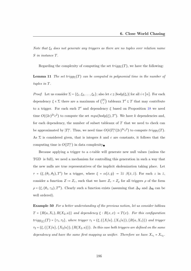
6. Close World Chasing
Note that ξ2 does not generate any triggers as there are no tuples over relation name
S in instance T .
Regarding the complexity of computing the set triggΣ(T ), we have the following:
Lemma 11 The set triggΣ(T ) can be computed in polynomial time in the number of
tuples in T .
Proof: Let us consider Σ = {ξ1, ξ2, . . . , ξk}; also let c ≥ ∣body(ξi)∣ for all i ∈ [n]. For each
dependency ξ ∈ Σ there are a maximum of (∣T ∣c) tableaux T ′ ⊆ T that may contribute
to a trigger. For each such T ′ and dependency ξ based on Proposition 18 we need
time O((2c)2cc2) to compute the set mgu(body(ξ), T ′). We have k dependencies and,
for each dependency, the number of subset tableaux of T that we need to check can
be approximated by ∣T ∣c. Thus, we need time O(k∣T ∣c(2c)2cc2) to compute triggΣ(T ).
As Σ is considered given, that is integers k and c are constants, it follows that the
computing time is O(∣T ∣c) in data complexity∎
Because applying a trigger to a c-table will generate new null values (unless the
TGD is full), we need a mechanism for controlling this generation in such a way that
the new nulls are true representatives of the implicit skolemization taking place. Let
τ = (ξ, (θ1, θ2), T ′) be a trigger, where ξ = α(x, y) → ∃z β(x, z). For each z in z,
consider a function Z ↦ Zτ , such that we have Zτ = Zρ for all triggers ρ of the form
ρ = (ξ, (θ1, γ2), T ′′). Clearly such a function exists (assuming that ΔV and ΔN can be
well ordered).
Example 50 For a better understanding of the previous notion, let us consider tableau
T = {R(a,X1),R(X2, a)} and dependency ξ ∶ R(x,x) → T (x). For this configuration
trigg{ξ}(T ) = {τ1, τ2}, where trigger τ1 = (ξ, ({X/a},{X1/a}),{R(a,X1)}) and trigger
τ2 = (ξ, ({X/a},{X2/a}),{R(X2, a)}). In this case both triggers are defined on the same
dependency and have the same first mapping as unifier. Therefore we have Xτ1 = Xτ2.
186

6. Close World Chasing
Before introducing the conditional-chase micro-step, let us clarify some useful no-
tations. Let (T,ϕ) be a conditional table. Then we define:
⩕(T,ϕ) =def ⋀t∈T
ϕ(t), (6.41)
Also, when θ is finite partial mapping from ΔN to the set ΔN ∪ΔC, we shall use
the abbreviation:
⩕(θ) =def ⋀i
Xi = θ(Xi), (6.42)
where the Xi’s are all the nulls in the domain of θ.
We are now ready to define the conditional-chase step on an conditional table with
a total order on its tuples.
Definition 46 Let (T,ϕ) be a conditional table that is a conditional core such that
there exists a total order ⋖ on its tuples. Let τ = (ξ, (θ1, θ2), T ′) be a trigger from
triggΣ(T ). We denote by θτ1 the extension of θ1 that maps each null Z from head(ξ)
associated with an existentially quantified variable z from ξ, to the variable Zτ . We say
that the conditional table (U,φ) is obtained from (T,ϕ) by applying trigger τ , if (U,φ)
contains all the c-tuples from T together with their possibly modified local conditions
and possibly a new c-tuple, as follows:
If T contains a tuple t syntactically equal to θτ1(head(ξ)),
then for (U,φ) the local condition of t is changed to:
φ(t) =def ϕ(t) ∨ (⩕ (T ′, ϕ) ∧⩕(θ2)), (6.43)
else add the tuple t′ ∶ θτ1(head(ξ)) with local condition:
φ(t′) =def ⩕(T ′, ϕ) ∧⩕(θ2) (6.44)
such that t⋖ t′ for all t ∈ T .
187

6. Close World Chasing
If (U,φ) is obtained from (T,ϕ), in this way we write (T,ϕ) →τ (V,ψ), where (V,ψ)
is the conditional table computed by CORE-COMP algorithm with input (U,φ). This
transformation is called a conditional-chase micro-step (or simply micro-step).
Note that in this case the lexicographic order between tuples cannot be used as we
may generate tuples that precede lexicographically the existing ones. In this case, an
index based order may be used, that is to each tuple is assigned an index (numerical
value) based on the total order in the initial conditional table and for each of the tuples
added by the micro-step the index is increased by 11.
The intuition behind computing the core of the conditional table at each micro-step
is given by the way constructible models semantics is defined (we want the conditional
chase to mimic the constructible models semantics). To exemplify this case, consider
the following example:
Example 51 Let us consider the conditional table without any local conditions (that
is a tableau) T = {R(a, b),R(a, c)}. Let Σ = {ξ1, ξ2}, where:
ξ1 ∶ R(x, y) → ∃z S(x, z) (6.45)
ξ2 ∶ S(x, y) → ∃z P (x, z) (6.46)
Supposing that the core computation for the conditional table is no needed, then we
have the following triggers in triggΣ(T, true):
τ1 = (ξ1, ({X/a, Y /b},{}),{R(a, b)}) and
τ2 = (ξ1, ({X/a, Y /c},{}),{R(a, c)}).
By applying these triggers according to Definition 46, it will create the following
new tuples: S(a,X1) and S(a,X2) with tautological local condition. These new tuples
1Note that this is the reason why the CORE-COMP algorithm traverses the tuples indescending order.
188
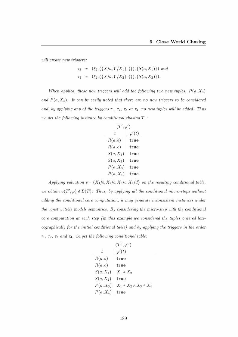
6. Close World Chasing
will create new triggers:
τ3 = (ξ2, ({X/a, Y /X1},{}),{S(a,X1)}) and
τ4 = (ξ2, ({X/a, Y /X2},{}),{S(a,X2)}).
When applied, these new triggers will add the following two new tuples: P (a,X3)
and P (a,X4). It can be easily noted that there are no new triggers to be considered
and, by applying any of the triggers τ1, τ2, τ3 or τ4, no new tuples will be added. Thus
we get the following instance by conditional chasing T :
(T ′, ϕ′)t ϕ′(t)
R(a, b) true
R(a, c) true
S(a,X1) true
S(a,X2) true
P (a,X3) true
P (a,X4) true
Applying valuation v = {X1/b,X2/b,X3/c,X4/d} on the resulting conditional table,
we obtain v(T ′, ϕ) ∉ Σ(T ). Thus, by applying all the conditional micro-steps without
adding the conditional core computation, it may generate inconsistent instances under
the constructible models semantics. By considering the micro-step with the conditional
core computation at each step (in this example we considered the tuples ordered lexi-
cographically for the initial conditional table) and by applying the triggers in the order
τ1, τ2, τ3 and τ4, we get the following conditional table:
(T ′′, ϕ′′)t ϕ′(t)
R(a, b) true
R(a, c) true
S(a,X1) X1 ≠ X2
S(a,X2) true
P (a,X3) X1 ≠ X2 ∧X3 ≠ X4
P (a,X4) true
189

6. Close World Chasing
The following lemma states, as expected, that a conditional micro-step is monotone
in the ⊑ partial order.
Lemma 12 If (T,ϕ) →τ (U,φ), then (T,ϕ) ⊑ (U,φ).
Proof: The proof is immediate from Definition 46 and Proposition 54∎
Having a table (T,ϕ) and a finite set Σ of TGD’s, the set of triggers triggΣ(T,ϕ)
is obviously finite. Consider a sequence
(T,ϕ) →τ1 (U1, ϕ1) →τ2 ⋯→τn (Un, ϕn),
where τ1, τ2, . . . , τn is an ordering of all the triggers from the set triggΣ(T,ϕ). We call
this a conditional-chase micro-sequence for (T,ϕ) using triggΣ(T,ϕ).
Example 52 Let us consider conditional table (T,ϕ):
(T,ϕ)t ϕ(t)
R(a, b) X1 = c
R(b, a) X2 = d
P (a, b) X3 = e
To this let us add dependencies Σ = {ξ1, ξ2}, where
ξ1 ∶ R(x, y) → ∃z S(x, z)
ξ2 ∶ P (x, y) → ∃R(x, y)
For (T,ϕ) and Σ, we have the following set of triggers triggΣ(T,ϕ):
τ1 = (ξ1, ({X/a, Y /b},{}),{R(a, b)})
τ2 = (ξ1, ({X/b, Y /a},{}),{R(b, a)})
τ3 = (ξ2, ({X/a, Y /b},{}),{P (b, a)})
190

6. Close World Chasing
Let us consider the following sequence of micro-steps, obtained by applying the trig-
gers τ1 followed by τ2 and τ3:
(T,ϕ) →τ1 (U1, ψ1) →τ2 (U2, ψ2) →τ3 (U3, ψ3).
where (U1, ψ1), (U2, ψ2) and (U3, ψ3) are the following conditional tables:
(U1, ψ1)t ψ1(t)
R(a, b) X1 = c
R(b, a) X2 = d
P (a, b) X3 = e
S(a, Y1) X1 = c
(U2, ψ2)t ψ2(t)
R(a, b) X1 = c
R(b, a) X2 = d
P (a, b) X3 = e
S(a, Y1) X1 = c
S(b, Y2) X2 = d
(U3, ψ3)t ψ3(t)
R(a, b) X1 = c ∨X3 = e
R(b, a) X2 = d
P (a, b) X3 = e
S(a, Y1) X1 = c
S(b, Y2) X2 = d
Let us now consider another sequence of micro-steps obtained by applying first τ2
followed by τ3 and τ1:
(T,ϕ) →τ2 (V1, μ1) →τ3 (V2, μ2) →τ1 (V3, μ3).
where (V1, μ1), (V2, μ2) and (V3, μ3) are the following conditional tables:
(V1, μ1)t μ1(t)
R(a, b) X1 = c
R(b, a) X2 = d
P (a, b) X3 = e
S(b, Y2) X2 = d
(V2, μ2)t μ2(t)
R(a, b) X1 = c ∨X3 = e
R(b, a) X2 = d
P (a, b) X3 = e
S(b, Y2) X2 = d
(V3, μ3)t μ3(t)
R(a, b) X1 = c ∨X3 = e
R(b, a) X2 = d
P (a, b) X3 = e
S(b, Y2) X2 = d
S(a, Y1) X1 = c ∨X3 = e
Note that even by applying the same set of triggers on conditional table (T,ϕ) we
have repC(U3, ψ3) ≠ repC(V3, μ3).
As it can be noted in the previous example, the order in which the triggers are
applied in a conditional micro-sequence does affect the outcome, but we shall see that
in the end the order will not matter.
191

6. Close World Chasing
After a micro-sequence, it is not guaranteed that the representation of the result
will satisfy the set of dependencies. It may be that additional triggers will be generated.
We therefore abstract a micro-sequence into a macro-step, as follows:
Definition 47 Let (T,ϕ) and (U,φ) be conditional tables with a total order on the set
of tuples; and let Σ be a set of TGD’s. We write (T,ϕ) ⇒Σ (U,φ), if (U,φ) is obtained
from (T,ϕ) by applying all micro-steps generated from triggΣ(T ). The transformation
from (T,ϕ) to (U,φ) is called a conditional-chase macro-step using Σ.
For the conditional table and the set of dependencies from Example 52, we have
the macro-steps (T,ϕ) ⇒Σ (U3, ψ3) and (T,ϕ) ⇒Σ (V3, μ3). It is a corollary of Lemma
12 that the macro-step is monotone.
Corollary 9 If (T,ϕ) ⇒Σ (U,φ), then (T,ϕ) ⊑ (U,φ).
We are now ready to introduce the concept of a conditional-chase sequence.
Definition 48 Let (T,ϕ) be a c-table and Σ a set of TGD’s. A sequence
(T0, ϕ0), (T1, ϕ1), . . . , (Tn, ϕn), . . .
of c-tables, inductively constructed as
(T0, ϕ0) = (T,ϕ),
(Ti+1, ϕi+1) = (U,φ), where (Ti, ϕi) ⇒Σ (U,φ),
(Tω, ϕω) = ⊔i∈ω
(Ti, ϕi),
is called a conditional-chase sequence associated with (T,ϕ) and Σ. We denote
chasecondΣ (T0, ϕ0) = (Tω, ϕω).
Note that the separation of micro and macro sequences guarantees that the overall
sequence will be fair, as all applicable trigger is fired in each micro sequence.
The following lemma follows directly from the definition of the triggers:
192
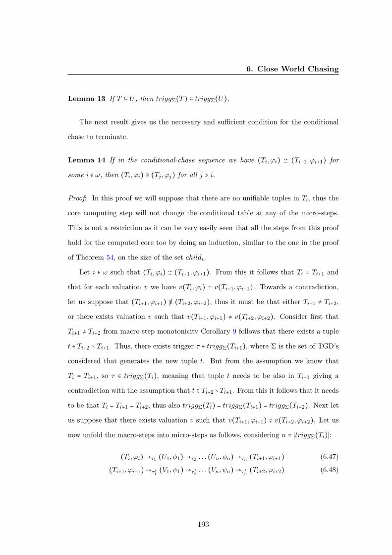
6. Close World Chasing
Lemma 13 If T ⊆ U , then triggΣ(T ) ⊆ triggΣ(U).
The next result gives us the necessary and sufficient condition for the conditional
chase to terminate.
Lemma 14 If in the conditional-chase sequence we have (Ti, ϕi) ≅ (Ti+1, ϕi+1) for
some i ∈ ω, then (Ti, ϕi) ≅ (Tj , ϕj) for all j > i.
Proof: In this proof we will suppose that there are no unifiable tuples in Ti, thus the
core computing step will not change the conditional table at any of the micro-steps.
This is not a restriction as it can be very easily seen that all the steps from this proof
hold for the computed core too by doing an induction, similar to the one in the proof
of Theorem 54, on the size of the set childv.
Let i ∈ ω such that (Ti, ϕi) ≅ (Ti+1, ϕi+1). From this it follows that Ti = Ti+1 and
that for each valuation v we have v(Ti, ϕi) = v(Ti+1, ϕi+1). Towards a contradiction,
let us suppose that (Ti+1, ϕi+1) /≅ (Ti+2, ϕi+2), thus it must be that either Ti+1 ≠ Ti+2,
or there exists valuation v such that v(Ti+1, ϕi+1) ≠ v(Ti+2, ϕi+2). Consider first that
Ti+1 ≠ Ti+2 from macro-step monotonicity Corollary 9 follows that there exists a tuple
t ∈ Ti+2 ∖ Ti+1. Thus, there exists trigger τ ∈ triggΣ(Ti+1), where Σ is the set of TGD’s
considered that generates the new tuple t. But from the assumption we know that
Ti = Ti+1, so τ ∈ triggΣ(Ti), meaning that tuple t needs to be also in Ti+1 giving a
contradiction with the assumption that t ∈ Ti+2∖Ti+1. From this it follows that it needs
to be that Ti = Ti+1 = Ti+2, thus also triggΣ(Ti) = triggΣ(Ti+1) = triggΣ(Ti+2). Next let
us suppose that there exists valuation v such that v(Ti+1, ϕi+1) ≠ v(Ti+2, ϕi+2). Let us
now unfold the macro-steps into micro-steps as follows, considering n = ∣triggΣ(Ti)∣:
(Ti, ϕi) →τ1 (U1, φ1) →τ2 . . . (Un, φn) →τn (Ti+1, ϕi+1) (6.47)
(Ti+1, ϕi+1) →τ ′1(V1, ψ1) →τ ′2
. . . (Vn, ψn) →τ ′n (Ti+2, ϕi+2) (6.48)
193
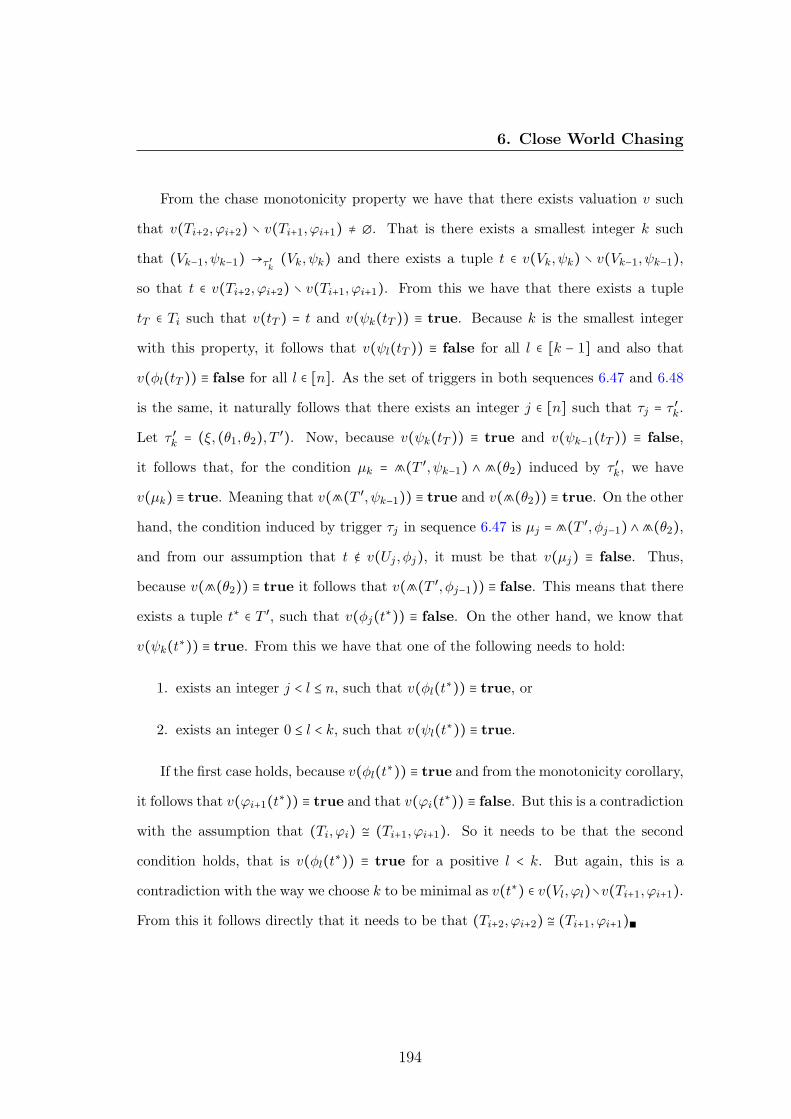
6. Close World Chasing
From the chase monotonicity property we have that there exists valuation v such
that v(Ti+2, ϕi+2) ∖ v(Ti+1, ϕi+1) ≠ ∅. That is there exists a smallest integer k such
that (Vk−1, ψk−1) →τ ′k(Vk, ψk) and there exists a tuple t ∈ v(Vk, ψk) ∖ v(Vk−1, ψk−1),
so that t ∈ v(Ti+2, ϕi+2) ∖ v(Ti+1, ϕi+1). From this we have that there exists a tuple
tT ∈ Ti such that v(tT ) = t and v(ψk(tT )) ≡ true. Because k is the smallest integer
with this property, it follows that v(ψl(tT )) ≡ false for all l ∈ [k − 1] and also that
v(φl(tT )) ≡ false for all l ∈ [n]. As the set of triggers in both sequences 6.47 and 6.48
is the same, it naturally follows that there exists an integer j ∈ [n] such that τj = τ ′k.
Let τ ′k = (ξ, (θ1, θ2), T ′). Now, because v(ψk(tT )) ≡ true and v(ψk−1(tT )) ≡ false,
it follows that, for the condition μk = ⩕(T ′, ψk−1) ∧ ⩕(θ2) induced by τ ′k, we have
v(μk) ≡ true. Meaning that v(⩕(T ′, ψk−1)) ≡ true and v(⩕(θ2)) ≡ true. On the other
hand, the condition induced by trigger τj in sequence 6.47 is μj = ⩕(T ′, φj−1) ∧⩕(θ2),
and from our assumption that t ∉ v(Uj , φj), it must be that v(μj) ≡ false. Thus,
because v(⩕(θ2)) ≡ true it follows that v(⩕(T ′, φj−1)) ≡ false. This means that there
exists a tuple t∗ ∈ T ′, such that v(φj(t∗)) ≡ false. On the other hand, we know that
v(ψk(t∗)) ≡ true. From this we have that one of the following needs to hold:
1. exists an integer j < l ≤ n, such that v(φl(t∗)) ≡ true, or
2. exists an integer 0 ≤ l < k, such that v(ψl(t∗)) ≡ true.
If the first case holds, because v(φl(t∗)) ≡ true and from the monotonicity corollary,
it follows that v(ϕi+1(t∗)) ≡ true and that v(ϕi(t∗)) ≡ false. But this is a contradiction
with the assumption that (Ti, ϕi) ≅ (Ti+1, ϕi+1). So it needs to be that the second
condition holds, that is v(φl(t∗)) ≡ true for a positive l < k. But again, this is a
contradiction with the way we choose k to be minimal as v(t∗) ∈ v(Vl, ϕl)∖v(Ti+1, ϕi+1).
From this it follows directly that it needs to be that (Ti+2, ϕi+2) ≅ (Ti+1, ϕi+1)∎
194

6. Close World Chasing
From the previous lemma it follows that, if for some i ∈ ω, (Ti, ϕi) ≅ (Ti+1, ϕi+1),
then we have (Tω, ϕω) ≅ (Ti, ϕi). In this case we say that the chase sequence converges
in the finite. From [3] we know that testing for two conditional tables if (Tω, ϕω) ≅
(Ti, ϕi) is ΠP2 -complete in general. In Section 6.5 we will present a class of dependencies
that ensures the conditional-chase termination in polynomial time without needing to
test the previous condition at each macro-step.
Example 53 Continuing with the conditional table and the triggers from Example 52
we have that (T,ϕ) ⇒Σ (T1, ϕ1), where (T1, ϕ1) is the conditional table (U3, ψ3) from
the given example. Applying the sets of triggers on (T1, ϕ1), we get the following micro-
step sequence:
(T1, ϕ1) →τ1 (U4, ψ4) →τ2 (U5, ψ5) →τ3 (T2, ϕ2).
Where (T2, ϕ2) is the following conditional table:
(T2, ϕ2)
t ϕ2(t)
R(a, b) X1 = c ∨X3 = e ∨X3 = e
R(b, a) X2 = d
P (a, b) X3 = e
S(a, Y1) X1 = c ∨ (X1 = c ∨X3 = e)
S(b, Y2) X2 = d ∨X2 = d
It is easy to check that (T1, ϕ1) /≅ (T2, ϕ2). Applying the triggers in the same
order yet another time, we get (T2, ϕ2) ⇒Σ (T3, ϕ3), where (T3, ϕ3) is the following
conditional table:
195

6. Close World Chasing
(T3, ϕ3)t ϕ3(t)
R(a, b) X1 = c ∨X3 = e ∨X3 = e ∨X3 = d
R(b, a) X2 = d
P (a, b) X3 = e
S(a, Y1) X1 = c ∨ (X1 = c ∨X3 = e) ∨ (X1 = c ∨X3 = e ∨X3 = e)S(b, Y2) X2 = d ∨X2 = d ∨X2 = d
In this case we have that (T2, ϕ2) ≅ (T3, ϕ3), so that (Tω, ϕω) = (T2, ϕ2). Thus the
result of the conditional chase was computed after three conditional macro-steps. Note
that if we would apply the triggers in the second order from the same Example 52, then
we would only need two macro steps to get to a congruent table to the one previously
obtained.
Next we proceed with a series of lemmas which allow us to prove the main prop-
erty of the conditional chase, namely that the representation of the conditional table
returned by the chase process is the same with the instance form the constructible
models semantics, i.e. repC(chasecondΣ (T,ϕ)) = Σ(repC(T,ϕ)).
Lemma 15 Let (T0, ϕ0) be a c-table, Σ a set of TGD’s , v a valuation for (T0, ϕ0),
I0 = v(T0, ϕ0) and G0 = ground(Σ). Also consider sequence:
(I0,G0) ⇒α1→β1 (I1,G1) ⇒α2→β2 ⋯⇒αn→βn (In,Gn) ⇒αn+1→βn+1 ⋯ (6.49)
and the unfolding of a conditional-chase sequence:
(T0, ϕ0) →τ1 (T1, ϕ1) →τ2 ⋯→τn (Tn, ϕn) →τn+1 ⋯ (6.50)
Then there exists a valuation v′, extending v, such that the following holds:
1. for any i ∈ ω (or i ∈ [n] if sequence 6.49 is finite of size n) there exists an integer
k such that Ii ⊆ v′(Tk, ϕk), and
196

6. Close World Chasing
2. for any j ∈ ω (or j ∈ [m] if sequence 6.50 is finite of size m) there exists an
integer k such that v′(Tj , ϕj) ⊆ Ik.
Proof: First we will inductively construct sequences v0 ⋐ v1 ⋐ . . . ⋐ vn ⋐ . . . and
(m0,m1, . . . ,mn, . . .) such that for any integer i we have (Ii, true) ⊆ vi(Tmi , ϕmi).
Intuitively, mi will be the index of the last micro-step from the unfold conditional-
chase sequence 6.50, used to compute valuation vi which is an extension of vi−1.
First we set v0 = v and m0 = 0 having I0 = v0(To, ϕ0). Let us suppose we constructed
sequences v0 ⋐ v1 ⋐ . . . ⋐ vk−1 and (m0, . . . ,mk−1) such that for all i ∈ [k − 1] we have
(Ii, true) ⊆ vi(Tmi , ϕmi).
We construct now vk as an extension of vk−1 as follows: let αk → βk ∈ ground(ξ) be
the k-th grounding applied in sequence 6.49. From the way a grounding is applied in the
constructible models semantics (see Section 6.2), we have that αk ⊆ Ik−1. But from the
inductive assumption and from the monotonicity of the conditional micro-step we have
that (Ik−1, true) ⊆ vk−1(Tj , ϕj) for any j ≥ k − 1. From this it follows that there exist
an integer j ≥ mk−1 and a trigger τj = (ξ, (θ1, θ2), T ′) ( guaranteed to exist because the
way macro-steps are defined), such that (θ1, θ2) is a more general unifier than (w, vk−1),
where w(body(ξ)) = αk, vk−1(T ′, ϕj−1) = αk and T ′ is a vk−1-core. Let θτj
1 (head(ξ))
be the new tuples generated by trigger τj . This means that there exists a valuation v′
such that v′(vk−1(θτj
1 (head(ξ)))) = βk. Otherwise, if such a valuation would not exist,
it would mean that trigger τj was already used in the inductive process with grounding
αl → βl, l < k where αl = αk. But this is a contradiction since, after applying the ground-
ing αl → βl, the set of grounding Gl does not contain any groundings of the form αl → ∗.
Let (Uj , ψj) be the c-table obtained from c-table (Tj−1, ϕj−1) by applying trigger τj ,
without computing the conditional core. Thus (Tj , ϕj) = CORE-COMP (Uj , ψj). We
know that vk−1(T ′, ϕj−1) ≡ true from the way (Uj , ψj) is constructed (see Definition
46), so it follows that vk−1(⩕(T ′, ϕj−1)) ≡ true. Also, because (θ1, θ2) is a more
197

6. Close World Chasing
general unifier than (w, vk−1), it follows that vk−1(⩕(θ2)) ≡ true. That is we have
βk ⊆ v′(vk−1(Uj , ψj)), thus because from the construction we have (Uj , ψj) ≅ (Tj , ϕj)
it follows that βk ∈ v′(vk−1(Tj , ϕj)) = v′(vk−1(Uj , ψj)). We now set vk = v′ ○ vk−1 and
mk = j. Clearly we have vk−1 ⋐ vj , mk > mk−1 and, because Ik = Ik−1 ∪ βk, we have
(Ik, true) ⊆ vk(Tmk, ϕmk
).
Let v′ = v0 ○ v1 ○ . . . ○ vn ○ . . .. We first show that for any integer k, if v′(Tk, ϕk)
is a ground instance, then there exists an integer j such that v′(Tk, ϕk) ⊆ Ij . We will
prove this by induction on k. For the base chase suppose k = 0. From the assumption
we have v′(T0, ϕ0) = v0(T0, ϕ0) = I0. Now let us suppose k > 0, v′(Tk, ϕk) is a ground
instance and for any l < k there exists an integer jl such that v′(Tl, ϕl) ⊆ Ijl. Towards a
contradiction, let us suppose that v′(Tk, ϕk) /⊆ Ii for any i ≥ 0. Let τk = (ξ, (θ1, θ2), T ′)
be the trigger from the chase sequence 6.50 used to obtain c-table (Tk, ϕk). Because,
from the induction assumption, v′(Tk−1, ϕk−1) ⊆ Ijl, it follows that it must be that
v′(θτk2 (head(ξ))) /⊆ Ii for any i > jl. Let v′(θτk
2 (head(ξ))) = β and v′(T ′, ϕk−1) = α,
clearly α ⊆ Ijl. Because (T ′, ϕk−1) is a core, it follows that for any T ′′ ⊆ Tk−1, T ′′ ≠ T ′
it cannot be that v′(T ′′, ϕk−1) = α. Thus, because α → β is never applied in sequence
6.49, it follows that there exists β′, different than β, such that α → β′ is applied in
the constructible models sequence. But because there is no tableau T ′′ ≠ T ′ such that
v′(T ′′, ϕk−1) = α, it follows that, when constructing v′, in the previous paragraph, for
grounding α → β′ we used the trigger τn = τk (it may be that we chose the trigger
when applied at step n not at step k), thus making v′(θτn2 (head(ξ))) = β′. But this is
a contradiction with the fact that v′(θτk2 (head(ξ))) = β and β ≠ β′.
In the previous paragraph we proved that, for any integer k, if v′(Tk, ϕk) is a
ground instance, then there exists an integer j such that v′(Tk, ϕk) ⊆ Ij . Now we will
show that, for any integer k, the valuation v′(Tk, ϕk) is a ground instance. Towards a
contradiction let us suppose that there exists an integer k such that v′(Tk, ϕk) is not a
198
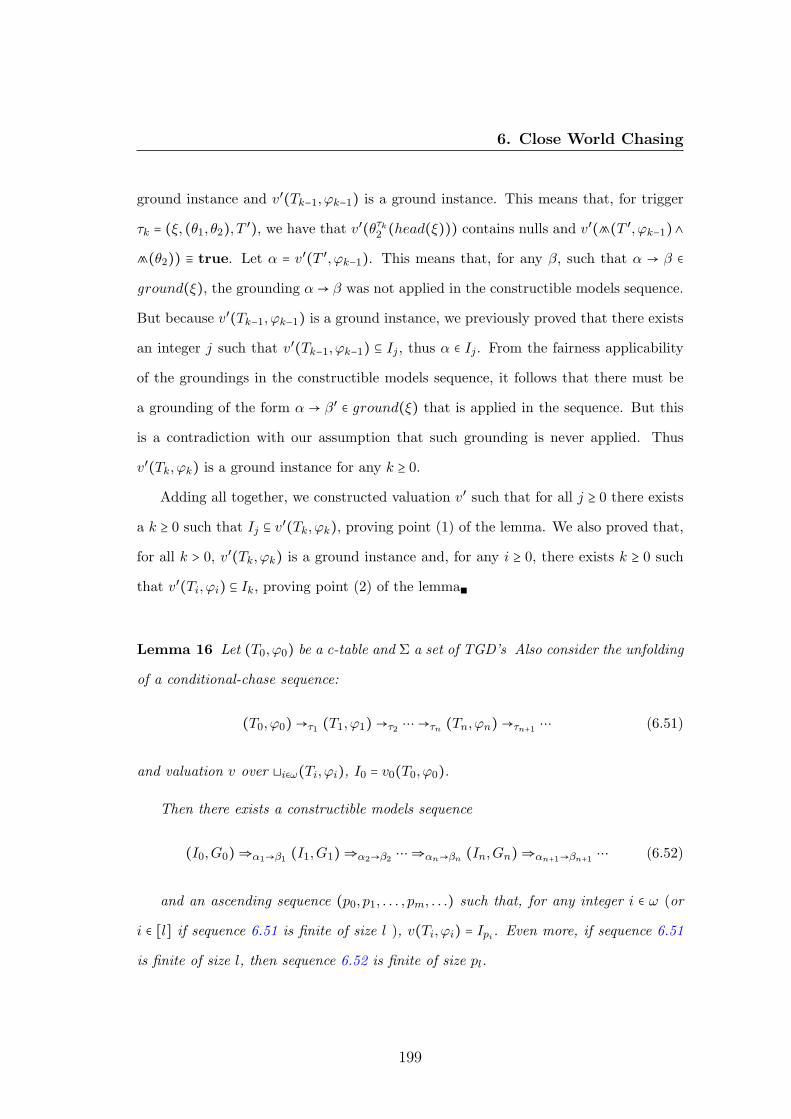
6. Close World Chasing
ground instance and v′(Tk−1, ϕk−1) is a ground instance. This means that, for trigger
τk = (ξ, (θ1, θ2), T ′), we have that v′(θτk2 (head(ξ))) contains nulls and v′(⩕(T ′, ϕk−1)∧
⩕(θ2)) ≡ true. Let α = v′(T ′, ϕk−1). This means that, for any β, such that α → β ∈
ground(ξ), the grounding α → β was not applied in the constructible models sequence.
But because v′(Tk−1, ϕk−1) is a ground instance, we previously proved that there exists
an integer j such that v′(Tk−1, ϕk−1) ⊆ Ij , thus α ∈ Ij . From the fairness applicability
of the groundings in the constructible models sequence, it follows that there must be
a grounding of the form α → β′ ∈ ground(ξ) that is applied in the sequence. But this
is a contradiction with our assumption that such grounding is never applied. Thus
v′(Tk, ϕk) is a ground instance for any k ≥ 0.
Adding all together, we constructed valuation v′ such that for all j ≥ 0 there exists
a k ≥ 0 such that Ij ⊆ v′(Tk, ϕk), proving point (1) of the lemma. We also proved that,
for all k > 0, v′(Tk, ϕk) is a ground instance and, for any i ≥ 0, there exists k ≥ 0 such
that v′(Ti, ϕi) ⊆ Ik, proving point (2) of the lemma∎
Lemma 16 Let (T0, ϕ0) be a c-table and Σ a set of TGD’s Also consider the unfolding
of a conditional-chase sequence:
(T0, ϕ0) →τ1 (T1, ϕ1) →τ2 ⋯→τn (Tn, ϕn) →τn+1 ⋯ (6.51)
and valuation v over ⊔i∈ω(Ti, ϕi), I0 = v0(T0, ϕ0).
Then there exists a constructible models sequence
(I0,G0) ⇒α1→β1 (I1,G1) ⇒α2→β2 ⋯⇒αn→βn (In,Gn) ⇒αn+1→βn+1 ⋯ (6.52)
and an ascending sequence (p0, p1, . . . , pm, . . .) such that, for any integer i ∈ ω (or
i ∈ [l] if sequence 6.51 is finite of size l ), v(Ti, ϕi) = Ipi. Even more, if sequence 6.51
is finite of size l, then sequence 6.52 is finite of size pl.
199

6. Close World Chasing
Proof: We will inductively construct the sequences 6.52 and (p0, p1, . . . , pm, . . .) based
on the number of micro-steps in 6.51. For the base case k = 0, we have I0 = v(T0, ϕ0),
thus p0 = 0. Let us suppose that k > 0. We have the ascending sequence (p0, p1, . . . , pk−1)
such that Ipi = v(Ti, ϕi), i ∈ [k − 1]. If v(Tk, ϕk) = v(Tk−1, ϕk−1), then we set pk = pk−1.
Thus, by induction assumption, we have Ipk= Ipk−1
= v(Tk−1, ϕk−1) = v(Tk, ϕk). Let us
now consider that v(Tk, ϕk) ≠ v(Tk−1, ϕk−1), from the monotonicity of the conditional
micro-steps it follows that v(Tk−1, ϕk−1) ⊂ v(Tk, ϕk). Let τk = (ξ, (θ1, θ2), T ′) be the
trigger used in 6.51 to generate c-table (Tk, ϕk) from (Tk−1, ϕk−1). Le us denote with
α = v(T ′, ϕk−1) and β = v(θτk2 (head(ξ))). Clearly we have v(Tk, ϕk) = v(Tk−1, ϕk−1)∪β,
and α ∈ v(Tk−1, ϕk−1) = Imk−1. It remains to be proved that the grounding α → β from
ground(ξ) is applicable on (Ipk−1,Gpk−1
). That is, we need to prove that α → β ∈ Gpk−1.
Towards a contradiction, let us suppose that α → β ∉ Gmk−1, thus in the sequence:
(I0,G0) ⇒α1→β1 (I1,G1) ⇒α2→β2 ⋯⇒αpk−1→βpk−1
(Ipk−1,Gpk−1
) (6.53)
there exists an integer j < k such that αpj = α. Let τj = (ξ, (θ′1, θ′2), T
′′) be the trigger
used at step j in the chase sequence 6.51. Clearly τj ≠ τk, otherwise they would generate
the same output instance. Following that, it needs to be that T ′′ ≠ T ′. Thus from the
monotonicity of the micro-step, it needs to be that there exists a tuple t′ ∈ T ′ ∖T ′′. On
the other hand, we also have that α = v(T ′, ϕk) = v(T ′′, ϕk), but from the micro-step
definition we have that all new tuples generated in T ′ succeeds (based on ⋖ order) the
tuples in T ′′. Because v(T ′, ϕk) = v(T ′′, ϕk) it follows that there exists a tuple t′′ ∈ T ′′,
such that v(t′) = v(t′′) and v(ϕk(t′)) ≡ true and v(ϕj(t′′)) ≡ true. Thus t′ and t′′ are
unifiable and t′′ ⋖ t′. On the other hand, because t′′ ⋖ t′, the CORE-COMP algorithm
adds a new conjunction to the local condition t′ not allowing it to be equal with t′′.
Following that, it cannot be that v(ϕk(t′)) ≡ true, beacuse it is a contradiction with
our previous assumption on tuple t′. From this, it follows that α → β is applicable on
200

6. Close World Chasing
(Ipk−1,Gpk−1
). We set pk = pk−1 + 1 and Ipk= Ipk−1
∪ β.
Let us now suppose that the conditional chase terminates after a chase sequence
of size l. Towards a contradiction let us suppose that there exists α → β ∈ ground(ξ)
such that α → β ∈ Gpland β /⊆ Ipl
. Because v(Tl, ϕl) = Ipl, this would mean that
there exists trigger τ = (ξ, (θ1, θ2), T ′) such that v(⩕(T ′, ϕl) ∧ ⩕(θ2)) ≡ true and
v(T ′, ϕl) = α. On the other hand, because in the chase sequence we would add another
step (Tl, ϕl) →τ (U,ψ), we would have that v(Tl, ϕl) = v(U,ψ), meaning that the
trigger τ = (ξ, (θ1, θ2), T ′) from the sequence 6.51 was already applied at step k ≤ l.
Consequently, in the constructible models sequence we would have eliminated α → ∗
from Gk, which means that Gl cannot have a grounding of the form α → ∗. This
contradicts with our assumption that such grounding exists. Therefore it must be that
the constructible models sequence is also finite and it has size pl∎
From the construction of the sequence (p0, p1, . . . , pm, . . .) in the previous proof,
it can be noted that sequence (1,2, . . . ,m, . . .) is a subsequence of (p0, p1, . . . , pm, . . .).
This is because it may be that pi = pi+1 for some i.
We are now ready to state the main theorem of this chapter, which says that the
result of the conditional chase represents exactly the constructible models.
Theorem 55 Let (T0, ϕ0) be a conditional table and Σ a set of TGD’s, then:
Σ(repC(T,ϕ)) = repC(chasecondΣ (T,ϕ)).
Proof: First we will show that Σ(repC(T,ϕ)) ⊆ repC(chasecondΣ (T,ϕ)). For this let
us consider I0 ∈ repC(T,ϕ), so there exists a valuation v such that v(T,ϕ) = I0. Now
let J ∈ Σ(I0), this means there exists a sequence:
(I0,G0) ⇒α1→β1 (I1,G1) ⇒α2→β2 ⋯⇒αn→βn (In,Gn) ⇒αn+1→βn+1 ⋯
201
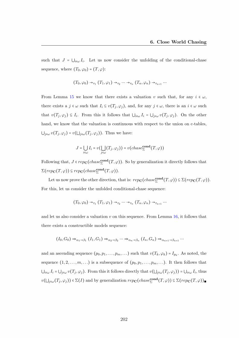
6. Close World Chasing
such that J = ⋃i∈ω Ii. Let us now consider the unfolding of the conditional-chase
sequence, where (T0, ϕ0) = (T,ϕ):
(T0, ϕ0) →τ1 (T1, ϕ1) →τ2 ⋯→τn (Tn, ϕn) →τn+1 ⋯
From Lemma 15 we know that there exists a valuation v such that, for any i ∈ ω,
there exists a j ∈ ω such that Ii ⊆ v(Tj , ϕj), and, for any j ∈ ω, there is an i ∈ ω such
that v(Tj , ϕj) ⊆ Ii. From this it follows that ⋃i∈ω Ii = ⋃j∈ω v(Tj , ϕj). On the other
hand, we know that the valuation is continuous with respect to the union on c-tables,
⋃j∈ω v(Tj , ϕj) = v(⊔j∈ω(Tj , ϕj)). Thus we have:
J = ⋃i∈ω
Ii = v(⊔j∈ω
(Tj , ϕj)) = v(chasecondΣ (T,ϕ))
Following that, J ∈ repC(chasecondΣ (T,ϕ)). So by generalization it directly follows that
Σ(repC(T,ϕ)) ⊆ repC(chasecondΣ (T,ϕ)).
Let us now prove the other direction, that is: repC(chasecondΣ (T,ϕ)) ⊆ Σ(repC(T,ϕ)).
For this, let us consider the unfolded conditional-chase sequence:
(T0, ϕ0) →τ1 (T1, ϕ1) →τ2 ⋯→τn (Tn, ϕn) →τn+1 ⋯
and let us also consider a valuation v on this sequence. From Lemma 16, it follows that
there exists a constructible models sequence:
(I0,G0) ⇒α1→β1 (I1,G1) ⇒α2→β2 ⋯⇒αn→βn (In,Gn) ⇒αn+1→βn+1 ⋯
and an ascending sequence (p0, p1, . . . , pm, . . .) such that v(Tk, ϕk) = Ipk. As noted, the
sequence (1,2, . . . ,m, . . .) is a subsequence of (p0, p1, . . . , pm, . . .). It then follows that
⋃i∈ω Ii = ⋃j∈ω v(Tj , ϕj). From this it follows directly that v(⊔j∈ω(Tj , ϕj)) = ⋃i∈ω Ii, thus
v(⊔j∈ω(Tj , ϕj)) ∈ Σ(I) and by generalization repC(chasecondΣ (T,ϕ)) ⊆ Σ(repC(T,ϕ))∎
202

6. Close World Chasing
A direct corollary of this theorem is that, by using conditional chase in data ex-
change, one may represent the target instance as a conditional table representing exactly
the solution space under constructible models semantics.
Corollary 10 Let M = (S,T,Σst,Σt) be a data exchange mapping and I be a ground
instance. If the conditional chase terminates with input I and Σ = Σst ∪Σt, then:
repC(chasecondΣ (I, true))∣T = SolCMM(I).
6.5 On Conditional-Chase Termination
In Chapter 4 we presented some classes of TGD’s which guarantee the termination
for different chase variations. In this section we will present a class of TGD’s which
guarantees the conditional-chase termination. Let us denote by CTcond∀∀ the class of
TGD’s such that for any Σ ∈ CTcond∀∀ the conditional-chase algorithm terminates with
any c-tables (T,ϕ) and Σ.
The following proposition shows that the conditional chase does not terminate for
a more larger class of TGD’s than the oblivious chase.
Proposition 19 CTcond∀∀ ⊊ CTobl
∀∀ .
Proof: For the subset part, it is easy to see that any conditional-chase sequence on
c-table (T,ϕ) with Σ set of TGD’s is a superset for the oblivious-chase sequence on
T and Σ. Thus, if the conditional chase terminates for all conditional tables on Σ, it
follows that the oblivious chase on all instances will terminate on Σ too. For the strict
inclusion part, let us consider Σ = {R(x, y, y) → ∃z, v R(x, z, v)}. Using the technique
in [59] it can easily be shown that the standard chase with Σ terminates on all instances.
From this and Theorem 3 it follows that the oblivious chase with Σ terminates on all
instances. Consider then the conditional chase starting with c-table {R(a, b, b)} (the
203

6. Close World Chasing
local condition of R(a, b, b) is true). The result of this chase can be represented by the
infinite conditional table below:
t ϕ(t)
R(a, b, b) true
R(a,X1,X2) true
R(a,X3,X4) X1 = X2
R(a,X5,X6) (X1 = X2) ∧ (X3 = X4). . . . . .
This proves the strict inclusion part as well∎
In order to obtain the sufficient condition for the conditional-chase termination,
we introduce a new rewriting of a set of TGD’s Σ, called disjoining, and denoted Σ.
Given a TGD ξ, we denote with ξ the same dependency, where for each variable x
repeated in the body we replace all occurrences, except the first, of x in the body
with a fresh new universally quantified variable. For instance, if ξ denotes the de-
pendency R(x, y, x),R(y, z, x) → ∃v,w R(x, v,w), then ξ will denote the dependency
R(x, y, x1),R(y1, z, x2) → ∃v,w R(x, v,w), where the subscripted variables are fresh.
The set Σ is then {ξ ∶ ξ ∈ Σ}.
There is of course a difference between the conditional and the oblivious chase: the
former may fire based on unifiers (θ1, θ2) and the latter based only on homomorphisms
θ1. From this observation we obtain the following lemma.
Lemma 17 chasecondΣ (T,ϕ) terminates if chaseobl
Σ(T ) terminates.
From Definition 4 we observe that the extended dependency graph for Σ can be
obtained from the extended dependency graph of Σ by deleting edges, thus we have:
Lemma 18 If Σ is a richly acyclic set of TGD’s, then Σ is also richly acyclic.
We now have the main result of this section
204

6. Close World Chasing
Theorem 56 RA⊊ CTcond∀∀ and for any Σ ∈RA and any conditional table (T,ϕ) there
is a polynomial that bounds the execution time of the conditional-chase algorithm with
(T,ϕ) and Σ.
Proof. Let (T,ϕ) be a conditional table and Σ a richly acyclic set of TGD’s. By
Lemma 18, the set Σ is also richly acyclic, and by Lemma 1, the set Σ is weakly acyclic.
By [27], chasestdΣ(T ) terminates in polynomial time. By Theorem 14, chaseobl
Σ(T ) also
terminates in polynomial time, and then by Theorem 3, chasecondΣ (T,ϕ) terminates in
polynomial time in size of (T,ϕ).
For the strict inclusion part, consider Σ = {R(x,x) → ∃y R(x, y)}. It is easy to
see that Σ ∉RA. On the other hand, for each tuple that is unified with the body of
the dependency a new tuple is created. But this new tuple contributes in creating a
new tuple if and only if it is the same as the initial tuple. Thus, the conditional-chase
procedure will terminate in maximum n macro steps, where n is the size of the input
conditional table∎
205

Chapter 7
Chasing with Second Order
Dependencies
The notion of representation systems describes structures that are algebraically closed
under queries. For example, complete instances are closed under FO queries. This
means that given any ground instance and any FO query, one may represent the result
of the query as a ground instance. Unfortunately, as clarified in Chapter 6, the previous
property does not hold when dealing with incomplete databases. Therefore, the recent
conclusions stipulate that the representation systems are also highly relevant in the
context of data exchange. In the previous section we also have showed that if the
data exchange mapping is specified by a richly acyclic set of TGD’s, then for each
source data specified by a conditional table, there exists a conditional table over the
target such that it can be used to get the certain and possible answers to any FO
query. Unfortunately, there are many mappings that cannot be specified by sets of
TGD’s and EGD’s. In this chapter, we will develop the previous result showing that
we can extend the previous class of mappings to ordinary SO dependencies which are
specified by source-to-target second order dependencies and by richly acyclic target
206

7. Chasing with Second Order Dependencies
TGD’s and EGD’s. Second order dependencies plays an important role in composing
schema mappings. They were first introduced by Fagin et al. in [29] for source to target
dependencies and it was proved that the class of SO-tgd’s is the right language for
mapping composition. Later on this language was extended by adding weakly acyclic
target dependencies as well by Arenas, Fagin and Nash [9].
7.1 Second Order Dependencies
We introduced in Section 6.2 the constructible models semantics for dependencies spec-
ified by a set of TGD’s. Here we extend this semantics for a higher class of dependencies
source-to-target second order dependencies. For this, let us first present the notions of
term and source-to-target second order dependencies.
Definition 49 Let x be a sequence of variables and f be a sequence of function symbols.
A term based on x and f is defined recursively as follows:
• every variable in x is a term;
• every 0-ary function symbol in f is a term;
• if f is a function symbol of arity k, then f(t1, . . . , tk) is a term, where all ti are
terms for i ∈ [k].
Definition 50 Given a source schema S and a distinct target schema T, a source-to-
target second order dependency is a formula of the form:
∃f1 . . .∃fm((∀x1(α1 → β1)) ∧ . . . ∧ (∀xn(αn → βn)))
where for each i ∈ [m] and each k ∈ [n]:
• fi is a function symbol;
207

7. Chasing with Second Order Dependencies
• αk is a conjunction of atoms R(y) or equalities t1 = t2. With R ∈ S, y contains
variables from xk and t1, t2 are terms based on variables from xi and functions
f1, . . . , fn;
• βk is a conjunction of atoms S(t), where S ∈ T and t are terms based on xk and
{f1, . . . , fm};
• each variable in xk occurs in some relational atomic formula in αk.
We denote by st-SO dependencies we denote the class of all source-to-target second
order dependencies.
The last item in the previous definition ensures the safeness of the dependency.
Thus, the formula:
∃f,∃g (∀x, y R(x, y), f(x) = g(y) → S(x, y)) ∧ (∀x, y R(x,x), f(x) = g(y) → T (x, y))
is not st-SO dependencies as the second dependency contains universally quantified
variable y which does not occur in any relational atomic formula in the body.
Given Σ a st-SO dependencies, a source instance I and a target instance J , we say
that (I, J) is a model for Σ, denoted by I ∪ J ⊧ Σ, if I ∪ J satisfies Σ in the standard
model theoretic sense.
Example 54 [29] Consider the source schema S = {Emp}, where Emp is a unary
relation containing a list of employees; and a target schema S = {Mgr,SelfMgr},
where Mgr is a binary relation for the employees; and their manager and relation
SelfMgr is a unary relation that maintains all the self managers. Let us also consider
st-SO dependencies:
∃f(∀e (Emp(e) → Mgr(e, f(e))) ∧ ∀e (Emp(e) ∧ (e = f(e)) → SelfMgr(e)))
208

7. Chasing with Second Order Dependencies
Intuitively, the dependencies mention that for each employee in Emp there exists a
manager given by the function f ; and if for an employee the manager is the same as
the employee ( e = f(e) ), then that employee is a self-manager. Consider, for example,
the following instances:
I1
Emp(john)
J1
Mgr(john,mike)
I2
Emp(john)Emp(ann)Emp(mike)
J2
Mgr(john,mike)Mgr(ann,mike)Mgr(mike,mike)SelfMgr(mike)
I3
Emp(john)Emp(ann)
J3
Mgr(john,mike)Mgr(ann,mike)Mgr(mike,mike)
I4
Emp(john)Emp(ann)Emp(mike)
J4
Mgr(john,mike)Mgr(ann,mike)Mgr(mike,mike)
In this example I1∪J1 ⊧ Σ, I2∪J2 ⊧ Σ, I3∪J3 ⊧ Σ, even if the tuple Mgr(mike,mike)
exists, there is no employee “mike“ under the source Emp relation. Finally, I4∪J4 /⊧ Σ
because there exists an employee “mike“ whose manager is himself, but there is no entry
for him in the SelfMgr relation.
The following example shows that the membership problem for st-SO dependencies
is NP-hard (i.e. Given I and Σ, does I ⊧ Σ? ).
Example 55 [29] Let us consider the followings schemata S = {E} and T = {D}; and
the following st-SO dependencies:
Σ ∶ ∃f (∀x, y E(x, y) → D(f(x), f(y)))
We will reduce now the problem of 3-colorability graph problem to the membership
problem: Is instance I ⊧ Σ? Consider a graph G = (V,E). We construct instance
209

7. Chasing with Second Order Dependencies
I as follows: for each edge (v1, v2) from G add tuple E(v1, v2) in I. Also consider
DI = {(g, y), (y, g), (g, b), (b, g), (b, y), (y, b)}, where g, b and y stand for colors green,
blue and yellow respectively.
It is obvious that, if there exists an interpretation for function f in Σ, then G is
3-colorable, as the interpretation for f gives the colors for the vertexes. Also clearly if
G is 3-colorable, then there exists an interpretation of f such that I ⊧ Σ.
Consider ΔF a countable set of function names and function arity that assigns an
integer for each function symbols in ΔF. A term over ΔF is defined recursively as
follows:
• any constant a ∈ ΔC is a term,
• any null a ∈ ΔC is a term,
• any function symbol f ∈ ΔF with arity(f) = 0 is a term,
• for any function symbol f ∈ ΔF with arity(f) = k, f(t1, t2, . . . , tk) is a term,
where for any i ∈ [k], ti are terms.
We extend the notion of instance to Skolem instance by allowing as elements in the
instance terms and not only constants and nulls.
Example 56 Consider f, g two function symbols from ΔF such that arity(f) = 2 and
arity(g) = 1. The following is a Skolem instance using the function symbols f and g:
I
R(a,X, b, Y )R(b, f(X,a), c, Y )R(g(Y ), f(a, a), c, f(a, g(X)))
Let Σ be st-SO dependencies:
210

7. Chasing with Second Order Dependencies
∃f1 . . .∃fm((∀x1(α1 → β1)) ∧ . . . ∧ (∀xn(αn → βn)))
For such st-SO dependencies we say that the size of Σ is n, denoted by ∣Σ∣. For
each dependency ξi ∶ ∀xi(αi → βi), we denote by body(ξi) to be the Skolem instance
that contains a tuple for each atom in αi, where each universally quantified variable
from xi is mapped by a fresh new null value; where αi is the formula obtained from αi
by replacing each equality atom by a new binary relational symbol E, called equality
relation. Similarly, we define the Skolem instance head(ξi).
Example 57 Let Σ be st-SO dependencies from example 54:
∃f(∀e (Emp(e) → Mgr(e, f(e))) ∧ ∀e (Emp(e) ∧ (e = f(e)) → SelfMgr(e)))
For this we have ∣Σ∣ = 2. If we consider ξ1 = ∀e (Emp(e) → Mgr(e, f(e))) and
ξ2 = ∀e (Emp(e) ∧ (e = f(e)) → SelfMgr(e)), then:
body(ξ1) = {Emp(X)}
head(ξ1) = {Mgr(X,f(X))}
body(ξ2) = {Emp(Y ),E(Y, f(Y ))}
head(ξ2) = {SelfMgr(Y )}
Note that even if in the st-SO dependencies both dependencies use universally quantified
variable e, this variable is mapped to a new null according to its scope. Thus, in
the scope of the first occurrence, e is mapped to null X and, in the scope of second
occurrence, it is mapped to Y .
211

7. Chasing with Second Order Dependencies
7.2 Extending Constructible Models Semantics
7.2.1 Adding EGD’s
Before extending our constructible models semantics (introduced in Section 6.2) to
include st-SO dependencies, we have to define the constructible models semantics for
a more general set of dependencies, namely sets of TGD’s and EGD’s. For this, let us
see how an EGD is applied on a node (I,G). Let ∀x α(x) → x = y be an EGD, where
x, y are variables in seqx. For this EGD, we define the set of groundings:
ground(∀x α(x) → x = y) = ⋃i∈ω, vi(x)≠vi(y)
{α(vi(x)) → %}
where vi, i ∈ ω, is an enumeration of all valuations from the set of variables from x to
the countable set ΔC. Given a set Σ = {ξ1, . . . , ξn} and a set of TGD’s and EGD’s,
we define the set of groundings ground(Σ) = ground(ξ1) ∪ . . . ∪ ground(ξn). Let I be
a ground instance and G a set of finitely generated ground dependencies from Σ. Let
I be an instance and (α → %) ∈ G be a grounding of an EGD ξ ∈ Σ, if α ⊆ I, then we
say that (I,G) fails with the grounding (α → %) and it is denoted as (I,G) ⇒α→a=b %.
Consider now the sequence:
(I0,G0), (I1,G1), . . . , (In,Gn), . . .
where ((I0,G0) = (I,G) and (Ii,Gi) ⇒∗ (Ii+1,Gi+1), where ∗ ∈ Gi is either an TGD
or EGD grounding. If there exists an integer i such that (Ii,Gi) ⇒α→� %, we say that
the sequence is failing. For a non-failing sequence it is obvious that Ii ⊆ Ii+1 and that
Gi ⊇ Gi+1 for each i ∈ ω. For the non-falling sequence, we define the limit of a chase
sequence as:
(⋃i∈ω
Ii,⋂i∈ω
Gi).
212

7. Chasing with Second Order Dependencies
Similarly to the TGDcase, we use the notation C(I,G) for the set of the limits
of all chase sequences originating from (I,G). With this we can define the set of all
constructible models of I and Σ as:
Σ(I) = {J ∶ (J,G) ∈ C(I, ground(Σ)),G ⊆ ground(Σ)}.
Example 58 Figure 7.1 represents the constructible models chase tree corresponding
to the instance I = {R(a),R(b)} and Σ containing the following TGD and EGD:
R(x) → ∃y S(x, y)
S(x, y) → x = y.
Figure 7.1: Chase tree with TGD’s and EGD’s
213

7. Chasing with Second Order Dependencies
7.2.2 Adding st-SO dependencies
Now we are ready to extend even more the notion of constructible models semantics in
such a way that it also allows st-SO dependencies. For this, let Σ be st-SO dependencies
of the form:
∃f1 . . .∃fm((∀x(α1 → β1)) ∧ . . . ∧ (∀xn(αn → βn))) (7.1)
and let F = {f1, . . . , fm} be the set of function symbols therein. Let F ♭ be an interpre-
tation of F in the universe of ΔC. We construct with F ♭ the set of groundings GF ♭ as
follows: for each ∀xi αi → βi in 7.1, for i ∈ [n] and for each valuation vj , j ∈ ω, for xi
with values in ΔC add grounding α′i → β′i to G. Where, α′
i and β′i are obtained from
αi and βi respectively by replacing recursively each variable x ∈ xi with the value vi(x)
and each term fk(a), where a is a sequence of constants, with the constant given by the
corresponding interpretation for fk in F ♭. We will not consider in GF ♭ the groundings
that have an equality of the form a = b in the body of the grounding, with a, b as two
distinct constants. Also, we will eliminate all the equalities of the form a = a from the
body of the grounding. Similarly, if there is a grounding α → β in GF ♭ such that there
exists an equality of the form a = b in the head, with a, b two distinct constants, the
grounding is replaced with α → %. Also, we eliminate from β all equalities of the form
a = a. Thus, there will be no groundings with equalities in GF ♭ .
Example 59 Let us also consider the same st-SO dependencies from Example 54:
∃f(∀e (Emp(e) → Mgr(e, f(e))) ∧ ∀e (Emp(e) ∧ (e = f(e)) → SelfMgr(e)))
Consider also F ♭1 that interprets f as identity function. The set GF ♭
1is defined under
this interpretation as the following TGD’s and EGD’s groundings:
214
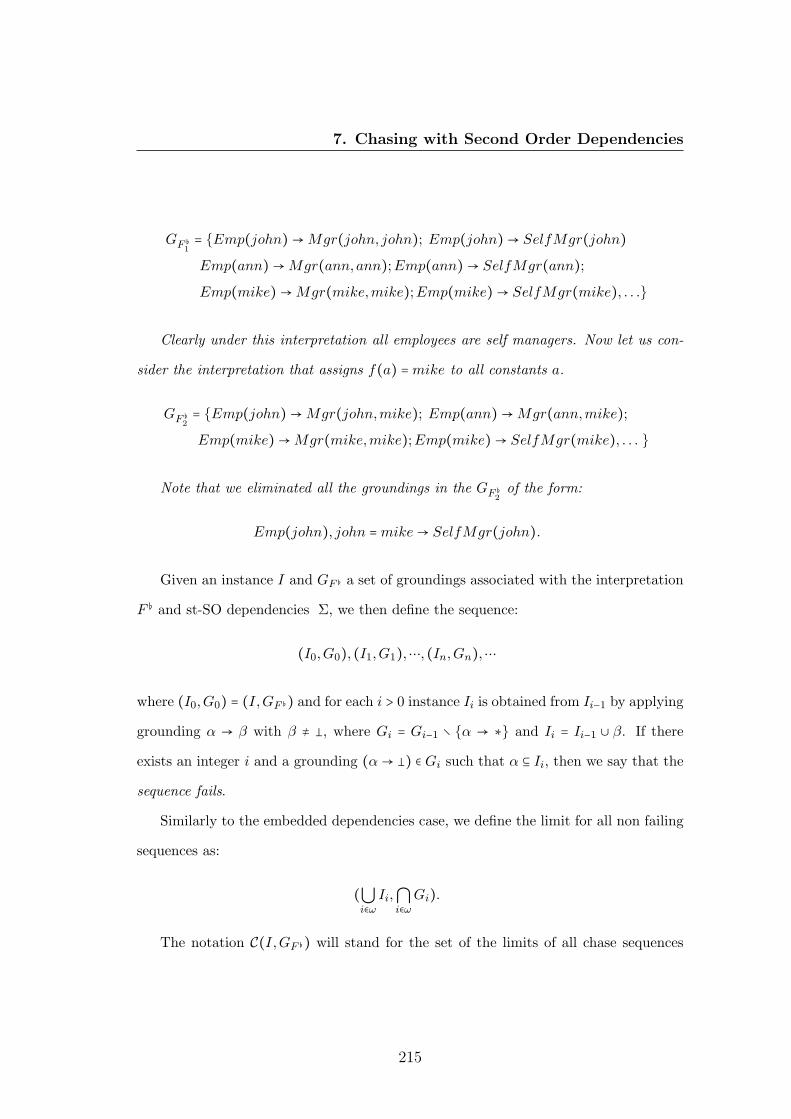
7. Chasing with Second Order Dependencies
GF ♭
1= {Emp(john) → Mgr(john, john); Emp(john) → SelfMgr(john)
Emp(ann) → Mgr(ann, ann);Emp(ann) → SelfMgr(ann);
Emp(mike) → Mgr(mike,mike);Emp(mike) → SelfMgr(mike), . . .}
Clearly under this interpretation all employees are self managers. Now let us con-
sider the interpretation that assigns f(a) = mike to all constants a.
GF ♭
2= {Emp(john) → Mgr(john,mike); Emp(ann) → Mgr(ann,mike);
Emp(mike) → Mgr(mike,mike);Emp(mike) → SelfMgr(mike), . . . }
Note that we eliminated all the groundings in the GF ♭
2of the form:
Emp(john), john = mike → SelfMgr(john).
Given an instance I and GF ♭ a set of groundings associated with the interpretation
F ♭ and st-SO dependencies Σ, we then define the sequence:
(I0,G0), (I1,G1),⋯, (In,Gn),⋯
where (I0,G0) = (I,GF ♭) and for each i > 0 instance Ii is obtained from Ii−1 by applying
grounding α → β with β ≠ %, where Gi = Gi−1 ∖ {α → ∗} and Ii = Ii−1 ∪ β. If there
exists an integer i and a grounding (α → %) ∈ Gi such that α ⊆ Ii, then we say that the
sequence fails.
Similarly to the embedded dependencies case, we define the limit for all non failing
sequences as:
(⋃i∈ω
Ii,⋂i∈ω
Gi).
The notation C(I,GF ♭) will stand for the set of the limits of all chase sequences
215

7. Chasing with Second Order Dependencies
originating from (I,GF ♭). We are now ready to defined ΣF ♭(I)
ΣF ♭(I) = {J ∶ (J,G) ∈ C(I,GF ♭)}
Finally for Σ a st-SO dependencies and I we define Σ(I) to be:
Σ(I) = ⋃F ♭ - interpretation
ΣF ♭(I)
Example 60 Continuing with the st-SO dependencies from Example 59, with the in-
terpretation F ♭1 and the instance I = {Emp(john),Emp(mike)}, we have:
ΣF ♭(I) = {{Emp(john),Emp(mike),Mgr(john, john),Mgr(mike,mike),
SelfMgr(john), SelfMgr(mike)}}
Given a mapping M = (S,T,Σ,∅), where Σ is a st-SO dependencies, and given a
source instance I, we extend the notion of constructible models solution space to st-SO
dependencies as follows:
SolCMM(I) = {J ∈ Inst(T)∣ ∃K ∈ Σ(I) and J = K ∣T}.
7.2.3 Adding st-SO dependencies and target TGD’s
We need to extend the constructible models semantics to allow, beside st-SO depen-
dencies, the target TGD’s. In order to achieve this, let us consider Σ = ΣstSO ∪ Σt,
where ΣstSO represents the st-SO dependencies and Σt identifies a set of TGD’s. Let
us denote by Gt the set of all groundings corresponding to Σt, as described in Section
6.2. For each interpretation F ♭ of the function symbols from ΣstSO, we consider the
set GF ♭ which corresponds to the source-to-target second order dependencies.
216

7. Chasing with Second Order Dependencies
Given an instance I and the sets of groundings GF ♭ associated with an interpretation
F ♭ and ΣstSO and Gt, we define the sequence:
(I0,G0), (I1,G1),⋯, (In,Gn)⋯
where (I0,G0) = (I,GF ♭ ∪Gt) and for each i > 0 instance Ii is obtained from Ii−1 by
applying the grounding α → β, where β ≠ %. In this case Gi = Gi−1 ∖ {α → ∗} and
Ii = Ii−1 ∪ β. In case there exist an integer i ≥ 0 and a grounding (α → %) ∈ Gi such
that α ⊆ Ii, then we say that the sequence fails. For a non failing sequence the limit is
defined as:
(⋃i∈ω
Ii,⋂i∈ω
Gi).
The notation C(I,GF ♭ ∪Gt) stands for the set of the limits of all chase sequences
originating from (I,GF ♭ ∪Gt). For Σ = ΣstSO ∪Σt, we define ΣF ♭(I):
ΣF ♭(I) = {J ∶ (J,G) ∈ C(I,GF ♭ ∪Gt)}
Finally, for Σ and I we define Σ(I) to be:
Σ(I) = ⋃F ♭ - interpretation
ΣF ♭(I)
The following proposition is a direct result of the fact that st-SO dependencies are
non-recursive. For a set of instances I, we define Σ(I) = ⋃I∈I Σ(I).
Proposition 20 Let S and T be two distinct schemata and let ΣstSO st-SO dependen-
cies and Σt be a set of target TGD’s. If Σ = ΣstSO ∪Σt, then:
Σ(I) = Σt(ΣstSO(I)).
Let M = (S,T,Σst,Σt) be a data exchange mapping, where Σst is specified by st-SO
dependencies, Σt is specified by a set of target TGD’s. Given a source instance I and
217

7. Chasing with Second Order Dependencies
by denoting Σ = Σst ∪Σt, we extend the notion of constructible models solution space
to st-SO dependencies and target TGD’s as follows:
SolCMM(I) = {J ∈ Inst(T)∣ ∃K ∈ Σ(I) and J = K ∣T}.
7.3 Global Conditional Tables
We present now an extension of the conditional tables (introduced in Section 6.3.1)
called global conditional tables [35]. As we will see in the following section, this ex-
tension is needed in order to capture the constructible models semantics over st-SO
dependencies.
A global conditional table (global c-table) is a pair (T,ϕ), where T is a tableau,
and ϕ, beside associating a local condition ϕ(t) with each tuple t ∈ T , it also associates
a global condition ϕ(T ) to (T,ϕ). Similarly to local conditions, the global condition
is a boolean formula built up from atoms of the form x = y, x ≠ y, x = a, x ≠ a,
a = b and a ≠ b for x, y ∈ ΔN, and a, b ∈ ΔC. An atomic equality of the form a = a for
a ∈ ΔC represents the logical constant true, while for two distinct constants a and b,
the equality a = b represents false.
A global conditional table (T,ϕ) represents a set of possible worlds. Let v be a
valuation such that v(ϕ(T )) ≡ true, then:
v(T,ϕ) = {v(t)∣ t ∈ T, and v(ϕ(t)) ≡ true}. (7.2)
The set of possible worlds represented by global c-table (T,ϕ) is:
repC(T,ϕ) = ⋃v, v(ϕ(T ))≡true
{v(T,ϕ)}. (7.3)
Note that any global conditional table (T,ϕ) with tautological global condition,
218

7. Chasing with Second Order Dependencies
that is for all valuation v we have v(ϕ(T )) ≡ true, is equivalent to the conditional
table (T,ϕ).
Example 61 Consider the global conditional table (T,ϕ) with the tabular representa-
tion shown below:
ϕ(T ) = (X = a ∨X = b ∨X = c)
t ϕ(t)
R(a,X) true
R(b, c) true
R(a, c) X = b
The set of possible worlds is given by the set of valuations for (T,ϕ) that makes the
global condition a tautology. The tabular representation of all the possible instances for
(T,ϕ), where Ii = vi(T,ϕ), for i ∈ {1,2,3}, v1(X) = a, v2(X) = b and v3(X) = c are
presented below:
I1
R(a, a)R(b, c)
I2
R(a, b)R(b, c)R(c, d)
I3
R(a, c)R(b, c)
The partial order “⊏“ is extended to the global conditional tables too. Let (T,ϕ)
and (U,ψ) be global c-tables. By (T,ϕ) ⊑ (U,φ) we mean that T ⊆ U , and that for all
valuations v such that v(ϕ(T )) ≡ true, it is that v(ϕ(U)) ≡ true and v(T,ϕ) ⊆ v(U,φ).
If both (T,ϕ) ⊑ (U,φ) and (T,ϕ) ⊑ (U,φ), we write (T,ϕ) ≅ (U,φ) and say that the
global c-tables are congruent.
Two global c-tables (T,ϕ), (U,φ) are said to be equivalent, denoted (T,ϕ) ≡ (U,φ),
if repC(T,ϕ) = repC(U,φ). Clearly Lemma 8 holds for global conditional tables as well.
The class of all global conditional tables is denoted by GCOND.
In the natural way, we extend the notion of conditional table and global conditional
table to the notions of Skolem conditional table and Skolem global conditional tables.
219
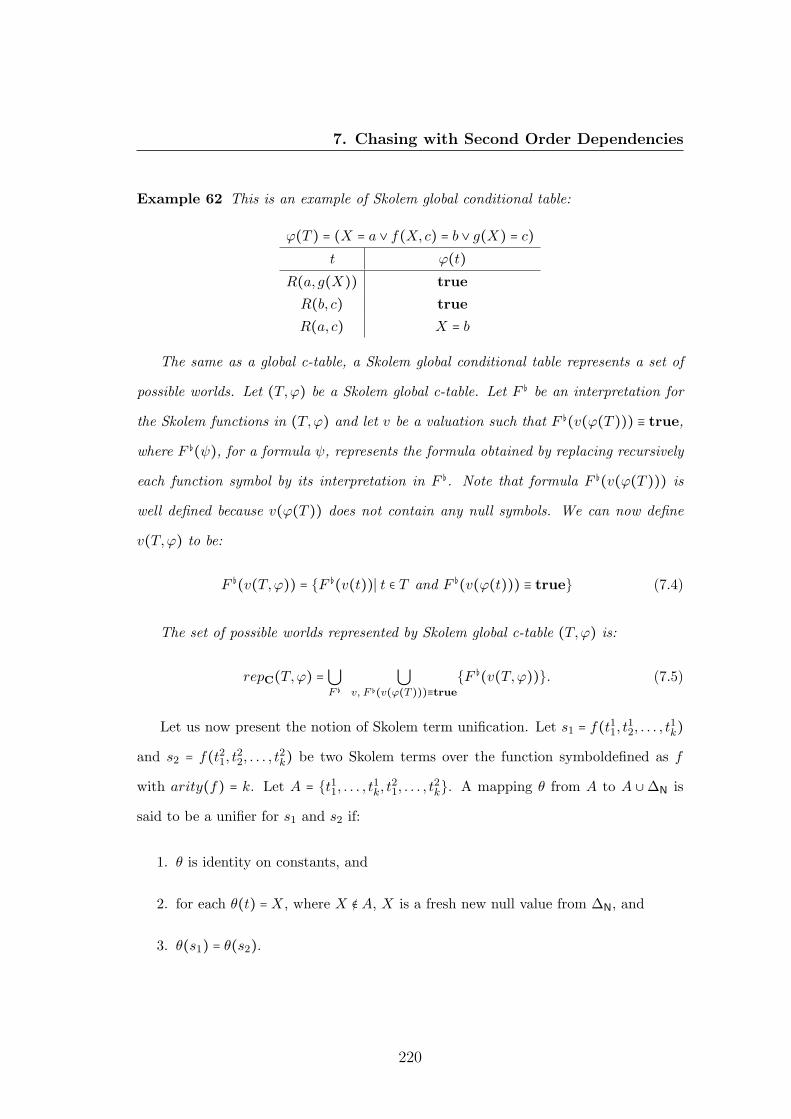
7. Chasing with Second Order Dependencies
Example 62 This is an example of Skolem global conditional table:
ϕ(T ) = (X = a ∨ f(X, c) = b ∨ g(X) = c)
t ϕ(t)
R(a, g(X)) true
R(b, c) true
R(a, c) X = b
The same as a global c-table, a Skolem global conditional table represents a set of
possible worlds. Let (T,ϕ) be a Skolem global c-table. Let F ♭ be an interpretation for
the Skolem functions in (T,ϕ) and let v be a valuation such that F ♭(v(ϕ(T ))) ≡ true,
where F ♭(ψ), for a formula ψ, represents the formula obtained by replacing recursively
each function symbol by its interpretation in F ♭. Note that formula F ♭(v(ϕ(T ))) is
well defined because v(ϕ(T )) does not contain any null symbols. We can now define
v(T,ϕ) to be:
F ♭(v(T,ϕ)) = {F ♭(v(t))∣ t ∈ T and F ♭(v(ϕ(t))) ≡ true} (7.4)
The set of possible worlds represented by Skolem global c-table (T,ϕ) is:
repC(T,ϕ) = ⋃F ♭
⋃v, F ♭(v(ϕ(T )))≡true
{F ♭(v(T,ϕ))}. (7.5)
Let us now present the notion of Skolem term unification. Let s1 = f(t11, t12, . . . , t
1k)
and s2 = f(t21, t22, . . . , t
2k) be two Skolem terms over the function symboldefined as f
with arity(f) = k. Let A = {t11, . . . , t1k, t
21, . . . , t
2k}. A mapping θ from A to A ∪ΔN is
said to be a unifier for s1 and s2 if:
1. θ is identity on constants, and
2. for each θ(t) = X, where X ∉ A, X is a fresh new null value from ΔN, and
3. θ(s1) = θ(s2).
220
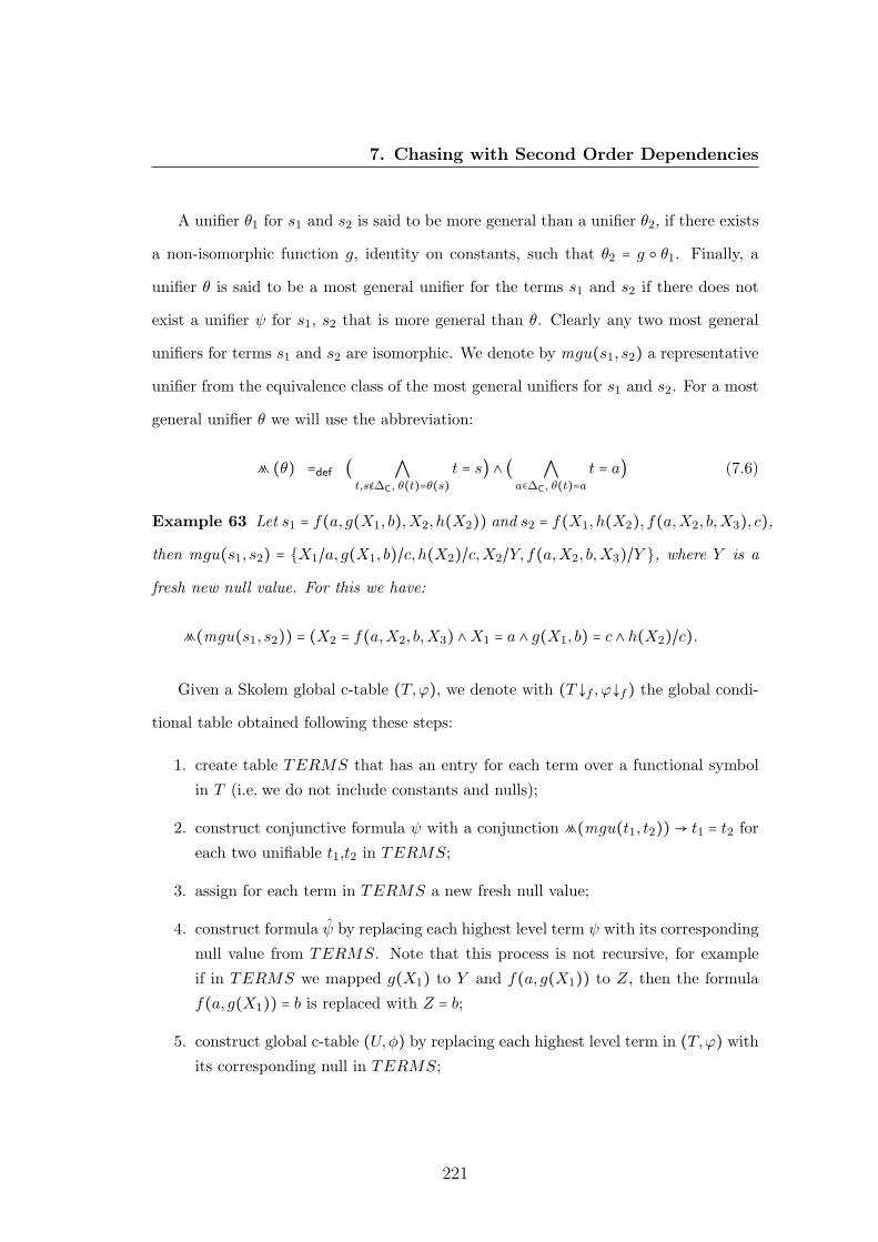
7. Chasing with Second Order Dependencies
A unifier θ1 for s1 and s2 is said to be more general than a unifier θ2, if there exists
a non-isomorphic function g, identity on constants, such that θ2 = g ○ θ1. Finally, a
unifier θ is said to be a most general unifier for the terms s1 and s2 if there does not
exist a unifier ψ for s1, s2 that is more general than θ. Clearly any two most general
unifiers for terms s1 and s2 are isomorphic. We denote by mgu(s1, s2) a representative
unifier from the equivalence class of the most general unifiers for s1 and s2. For a most
general unifier θ we will use the abbreviation:
F (θ) =def ( ⋀t,s∉ΔC, θ(t)=θ(s)
t = s) ∧ ( ⋀a∈ΔC, θ(t)=a
t = a) (7.6)
Example 63 Let s1 = f(a, g(X1, b),X2, h(X2)) and s2 = f(X1, h(X2), f(a,X2, b,X3), c),
then mgu(s1, s2) = {X1/a, g(X1, b)/c, h(X2)/c,X2/Y, f(a,X2, b,X3)/Y }, where Y is a
fresh new null value. For this we have:
F(mgu(s1, s2)) = (X2 = f(a,X2, b,X3) ∧X1 = a ∧ g(X1, b) = c ∧ h(X2)/c).
Given a Skolem global c-table (T,ϕ), we denote with (T ↓f , ϕ↓f) the global condi-
tional table obtained following these steps:
1. create table TERMS that has an entry for each term over a functional symbol
in T (i.e. we do not include constants and nulls);
2. construct conjunctive formula ψ with a conjunction F(mgu(t1, t2)) → t1 = t2 for
each two unifiable t1,t2 in TERMS;
3. assign for each term in TERMS a new fresh null value;
4. construct formula ψ by replacing each highest level term ψ with its corresponding
null value from TERMS. Note that this process is not recursive, for example
if in TERMS we mapped g(X1) to Y and f(a, g(X1)) to Z, then the formula
f(a, g(X1)) = b is replaced with Z = b;
5. construct global c-table (U,φ) by replacing each highest level term in (T,ϕ) with
its corresponding null in TERMS;
221

7. Chasing with Second Order Dependencies
6. construct (T ↓f , ϕ↓f) such that T ↓f= U and for all t ∈ T ↓f we have ϕ↓f (t) = φ(t)and ϕ↓f (T ↓f) = φ(U) ∧ ψ.
Because TERMS contains all the Skolem terms over the function symbols, it follows
that (T ↓f , ϕ ↓f) does not contain any function symbols, thus (T ↓f , ϕ ↓f) is a global
c-table.
Example 64 Let us exemplify the previous construction by considering (T,ϕ) to be
the following Skolemized global c-table:
ϕ(T ) = true
t ϕ(t)
R(a, f(X1, g(X2))) g(a) = f(a, b)R(b,X1) f(a, f(a, b)) = c
R(f(a, g(X3)), c) X = b
Under this setting the table TERMS will contain the following set of terms:
{f(X1, g(X2)), f(a, g(X3)), f(a, f(a, b)), f(a, b), g(X2), g(X3), g(a)}
Formula ψ obtained by unifying each term from TERMS will be:
ψ = (X1 = a ∧ g(X2) = g(X3) → f(X1, g(X2)) = f(a, g(X3)))
∧(X1 = a ∧ g(X2) = f(a, b) → f(X1, g(X2)) = f(a, f(a, b)))
∧(X1 = a ∧ g(X2) = b → f(X1, g(X2)) = f(a, b))
∧(g(X3) = f(a, b) → f(a, g(X3)) = f(a, f(a, b)))
∧(g(X3) = b → f(a, g(X3)) = f(a, b))
∧(f(a, b) = b → f(a, f(a, b)) = f(a, b))
∧(X2 = X3 → g(X2) = g(X3))
∧(X2 = a → g(X2) = g(a))
∧(X3 = a → g(X3) = g(a))
Next we assign a fresh new variable for each term in terms as follows:
222

7. Chasing with Second Order Dependencies
TERMS
f(X1, g(X2)) Y1
f(a, g(X3)) Y2
f(a, f(a, b)) Y3
f(a, b) Y4
g(X2) Y5
g(X3) Y6
g(a) Y7
Due to these notations, the formula ψ is transformed in ψ:
ψ = (X1 = a ∧ Y5 = Y6 → Y1 = Y2) ∧ (X1 = a ∧ Y5 = Y4) → Y1 = Y3)
∧(X1 = a ∧ Y5 = b → Y1 = Y4) ∧ (Y6 = Y4 → Y2 = Y3)
∧(Y6 = b → Y2 = Y4) ∧ (Y4 = b → Y3 = Y4)
∧(X2 = X3 → Y5 = Y6) ∧ (X2 = a → Y5 = Y7) ∧ (X3 = a → Y6 = Y7)
Thus, the global c-table (T ↓f , ϕ↓f) is:
ϕ↓f (T ↓f) = ψ
t ϕ↓f (t)
R(a, Y1) Y7 = Y4
R(b,X1) Y3 = c
R(Y2, c) X = b
The following theorem tells us that by removing the function symbols as presented
before, we do not loose any information.
Theorem 57 Given (T,ϕ) a Skolemized global c-table, then
repC(T,ϕ) = repC(T ↓f , ϕ↓f).
Proof: Let I ∈ repC(T,ϕ). This means there exists an interpretation F ♭ for the
function symbols in (T,ϕ) and the valuation v such that F ♭(v(ϕ(T ))) ≡ true and
I = F ♭(v(T,ϕ)). Let v′ be the valuation that extends v as follows: for each term t
223

7. Chasing with Second Order Dependencies
in TERMS associated with the null value Y we set v′(Y ) = F ♭(v(t)). Let us also
define ϕ↓f (T ) = φ(U) ∧ ψ (from the description of (T ↓f , ϕ↓f)). Now, from the used
construction, we have v′(φ(U)) = F ♭(ϕ(T )), thus v′(φ(U)) ≡ true. Let us consider a
conjunction α → Yi = Yj from ψ. Let us now replace Yi and Yj with the corresponding
terms ti and tj from TERMS. Thus, the formula becomes F(mgu(ti, tj)) → ti = tj .
But, from the construction of F(mgu(ti, tj)), it naturally follows that for any mapping
g such that g(F(mgu(ti, tj))) ≡ true, it is that g(ti) = g(tj). On the other hand, if
v(F(mgu(ti, tj))) ≡ true, from the construction of v′ we have that v′(α) ≡ true, and
also because v(ti) = v(tj) and because F ♭ is a well defined interpretation it follows that
v′(Yi) = v′(Yj). Thus, v′(α → Yi = Yj) ≡ true, meaning that v′(ϕ↓f (T ↓f)) ≡ true.
Now let t ∈ T . From the construction of (T ↓f , ϕ ↓f) it follows that there ex-
ists a tuple t′ ∈ T ↓f obtained from t by replacing each function symbols terms with
their corresponding null from TERMS table. Clearly, from the construction of v′,
we have that F ♭(v(t)) = v′(t′) and also that F ♭(v(ϕ(t))) = v′(ϕ ↓f (t′)). From
this it directly follows that F ♭(v(T,ϕ)) ⊆ v′(T ↓f , ϕ ↓f). Thus, by generalization,
repC(T,ϕ) ⊆ repC(T ↓f , ϕ↓f).
For the other direction, let us consider I ∈ repC(T ↓f , ϕ↓f). This means that there
exists a valuation v′ such that v′(ϕ↓f (T ↓f)) ≡ true. Let us set v to be the restriction
of v′ to all null values except the ones from TERMS. And let us define the inter-
pretation F ♭ such that for each term ti in TERMS with the associated labeled null
Yi set F ♭(v(ti)) = v′(Yi). Because v′(ψ) ≡ true, it follows that F ♭ is a well defined
interpretation. From this it follows, similarly to the proof for the other direction, that
v′(T ↓f , ϕ↓f) = F ♭(v(T,ϕ)) and, by generalization, that repC(T ↓f , ϕ↓f) ⊆ repC(T,ϕ)∎
224

7. Chasing with Second Order Dependencies
7.4 Chasing with Second Order Dependencies
In this section we will extend the conditional table chase with TGD’s to the global-
conditional chase with st-SO dependencies. To achieve this, first we need to extend
the tableau unification process to Skolem tableaux. For a Skolem tableau T , by T
we denote the tableau T restricted to all relational symbols except E. We denote by
ΔF(T ) the set of all terms in T . The homomorphism notion is extended in the natural
way to the Skolem tableaux too.
Definition 51 Let T and U be two Skolem tableaux such that only T may contain the
equality symbol E. A unifier for T and U , if it exists, is a pair (θ1, θ2), where θ1 is a
homomorphism from the set of terms ΔF(T ) to the set ΔF(U) ∪ΔC(dom(T )) and θ2
is a ΔC(dom(T ))-retraction for U , such that the following holds θ1(T ) = θ2(U).
Example 65 Consider tableau T = {R(a, f(X1), f(X1),X2),E(a, f(X1))} and tableau
U = {R(Y1, b, g(Y2), Y3)}. The pair (θ1, θ2), with the mappings θ1 = {f(X1)/b,X2/c}
and θ2 = {Y1/a, g(Y2)/b, Y3/c}, is a unifier for T and U . Another unifier for T and U
is (θ′1, θ′2), where θ′1 = {f(X1)/b,X2/Y3} and θ2 = {Y1/a, g(Y2)/b}.
Definition 52 A unifier (θ1, θ2) for the Skolem tableaux T and U is more general than
a unifier (γ1, γ2), if there is a mapping f on dom(U), f ∉ Id, identity on constants,
such that γ1 = f ○ θ1 and γ2 = f ○ θ2.
The more general unifier definition is extended to the most general unifier as follows:
Definition 53 A unifier (θ1, θ2) is a most general unifier (mgu) for the Skolem in-
stances T and U , if all unifiers (γ1, γ2) of T and U that are more general than (θ1, θ2)
actually are isomorphic with (θ1, θ2). We denote by mgu(T,U) the set of (representa-
tives of the) equivalence classes of all mgu’s of T and U .
225

7. Chasing with Second Order Dependencies
The same as in the standard-conditional chase case, we need to introduce the notion
of Skolemized conditional trigger.
Definition 54 Let Σ be st-SO dependencies of the form: ∃f ξ1, . . . , ξn, where each
ξi are of the form ∀xi αi → βi, for i ∈ [n]. Let T be a Skolem instance. A Skolem
conditional trigger for Σ on T (or simply a trigger) is a tuple τ = (ξi, θ, T′), where
i ∈ [n] and θ = (θ1, θ2) is a mgu that unifies body(ξi) with T ′, where T ′ ⊆ T , and T ′ is
a θ2-core. The set triggΣ(T ) contains the set of all triggers for Σ on T .
Example 66 Going back to st-SO dependencies, from Example 54:
∃f(∀e (Emp(e) → Mgr(e, f(e))) ∧ ∀e (Emp(e) ∧ (e = f(e)) → SelfMgr(e)))
Let ξ1 = ∀e (Emp(e) → Mgr(e, f(e))) and ξ2 = ∀e (Emp(e)∧(e = f(e)) → SelfMgr(e)).
Consider a tableau T = {Emp(john),Emp(mike)}. For this configuration we have the
following set of triggers:
τ1 = (ξ1, ({e/john},{}),{Emp(john)})
τ2 = (ξ2, ({e/john},{}),{Emp(john)})
τ1 = (ξ1, ({e/mike},{}),{Emp(mike)})
τ2 = (ξ2, ({e/mike},{}),{Emp(mike)})
Note that when dealing with st-SO dependencies there are no existentially quanti-
fied variables, so there is no need to create new null values during the chase process. It
can also be observed that the presence of the Skolem functions ease the chase process
as there is no need anymore to compute the core for the conditional table.
Before introducing the Skolem-conditional chase micro-step, let us introduce some
notations similar to the ones presented for the conditional-chase process introduced in
Section 6.4. Let (T,ϕ) be a Skolem conditional table. Then we define:
226

7. Chasing with Second Order Dependencies
⩕ (T,ϕ) =def ⋀t∈T
ϕ(t), (7.7)
When θ is a finite partial mapping from ΔN to the set ΔN ∪ΔC, we shall use the
abbreviation:
⩕ (θ) =def ⋀i
Xi = θ(Xi), (7.8)
where the Xi’s are all the nulls in the domain of θ.
For a Skolem trigger τ = (ξ, (θ1, θ2), T ′) we define:
⩕L (τ) =def ⋀E(t1,t2)∈body(ξ)
θ1(t1) = θ1(t2), (7.9)
⩕G (τ) =def ⋀E(t1,t2)∈head(ξ)
⩕(θ2) ∧⩕(T ′, ϕ) ∧⩕L(τ) → θ1(t1) = θ1(t2). (7.10)
These new notations are now useful to define the conditional-chase step on the
Skolem conditional tables:
Definition 55 Let (T,ϕ) be a Skolem conditional table. Let τ = (ξ, (θ1, θ2), T ′) be a
trigger from triggΣ(T ). We say that the Skolem conditional table (U,φ) is obtained
from (T,ϕ) by applying trigger τ , if (U,φ) contains all the c-tuples from T together
with their possibly modified local and global conditions, and possibly a new c-tuple, as
follows:
227
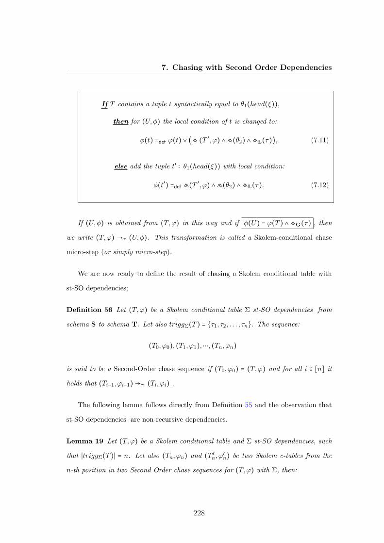
7. Chasing with Second Order Dependencies
If T contains a tuple t syntactically equal to θ1(head(ξ)),
then for (U,φ) the local condition of t is changed to:
φ(t) =def ϕ(t) ∨ (⩕ (T ′, ϕ) ∧⩕(θ2) ∧⩕L(τ)), (7.11)
else add the tuple t′ ∶ θ1(head(ξ)) with local condition:
φ(t′) =def ⩕(T ′, ϕ) ∧⩕(θ2) ∧⩕L(τ). (7.12)
If (U,φ) is obtained from (T,ϕ) in this way and if φ(U) = ϕ(T ) ∧⩕G(τ) , then
we write (T,ϕ) →τ (U,φ). This transformation is called a Skolem-conditional chase
micro-step (or simply micro-step).
We are now ready to define the result of chasing a Skolem conditional table with
st-SO dependencies;
Definition 56 Let (T,ϕ) be a Skolem conditional table Σ st-SO dependencies from
schema S to schema T. Let also triggΣ(T ) = {τ1, τ2, . . . , τn}. The sequence:
(T0, ϕ0), (T1, ϕ1),⋯, (Tn, ϕn)
is said to be a Second-Order chase sequence if (T0, ϕ0) = (T,ϕ) and for all i ∈ [n] it
holds that (Ti−1, ϕi−1) →τi (Ti, ϕi) .
The following lemma follows directly from Definition 55 and the observation that
st-SO dependencies are non-recursive dependencies.
Lemma 19 Let (T,ϕ) be a Skolem conditional table and Σ st-SO dependencies, such
that ∣triggΣ(T )∣ = n. Let also (Tn, ϕn) and (T ′n, ϕ′
n) be two Skolem c-tables from the
n-th position in two Second Order chase sequences for (T,ϕ) with Σ, then:
228
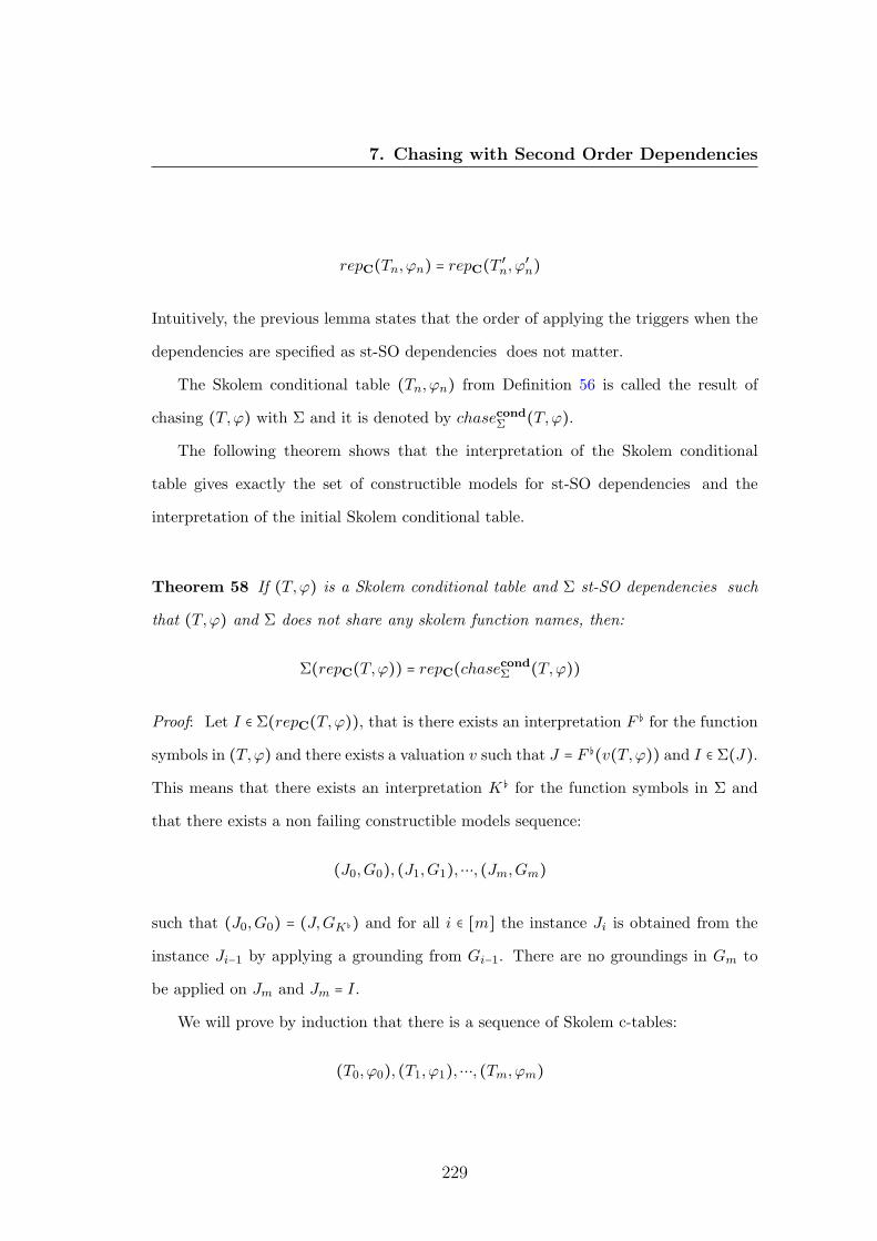
7. Chasing with Second Order Dependencies
repC(Tn, ϕn) = repC(T ′n, ϕ′
n)
Intuitively, the previous lemma states that the order of applying the triggers when the
dependencies are specified as st-SO dependencies does not matter.
The Skolem conditional table (Tn, ϕn) from Definition 56 is called the result of
chasing (T,ϕ) with Σ and it is denoted by chasecondΣ (T,ϕ).
The following theorem shows that the interpretation of the Skolem conditional
table gives exactly the set of constructible models for st-SO dependencies and the
interpretation of the initial Skolem conditional table.
Theorem 58 If (T,ϕ) is a Skolem conditional table and Σ st-SO dependencies such
that (T,ϕ) and Σ does not share any skolem function names, then:
Σ(repC(T,ϕ)) = repC(chasecondΣ (T,ϕ))
Proof: Let I ∈ Σ(repC(T,ϕ)), that is there exists an interpretation F ♭ for the function
symbols in (T,ϕ) and there exists a valuation v such that J = F ♭(v(T,ϕ)) and I ∈ Σ(J).
This means that there exists an interpretation K♭ for the function symbols in Σ and
that there exists a non failing constructible models sequence:
(J0,G0), (J1,G1),⋯, (Jm,Gm)
such that (J0,G0) = (J,GK♭) and for all i ∈ [m] the instance Ji is obtained from the
instance Ji−1 by applying a grounding from Gi−1. There are no groundings in Gm to
be applied on Jm and Jm = I.
We will prove by induction that there is a sequence of Skolem c-tables:
(T0, ϕ0), (T1, ϕ1),⋯, (Tm, ϕm)
229
7. Chasing with Second Order Dependencies
such that (T0, ϕ0) = (T,ϕ) and for each i ∈ [m], K♭(F ♭(v(Ti, ϕi))) = Ji.
For the base case, let us consider i = 0, from the hypothesis J = J0 = F ♭(v(T0, ϕ0)).
But since (T0, ϕ0) = (T,ϕ) and because there are no common Skolem functions in Σ
and (T,ϕ), it follows that J0 = K♭(F ♭(v(T0, ϕ0))), proving the base case.
For the induction step, let us consider that for any integer i ∈ [k − 1], for a k ∈ [m],
the induction assumption holds. We need to prove that K♭(F ♭(v(Tk, ϕk))) = Jk.
Now, let (Jk−1,Gk−1) ⇒α→β (Jk,Gk). Thus (α → β) ∈ ground(ξ), α ⊆ Jk−1 and
Jk = Jk−1 ∪ β. Because α ⊆ Jk−1 and from the induction assumption we have that
Jk−1 = K♭(F ♭(v(Tk−1, ϕk−1))). Therefore, there exists a subset minimal T ′ ⊆ Tk−1 such
that α = K♭(F ♭(v(T ′, ϕk−1))). Moreover, α is K♭(v′(body(ξ))) restricted to all relation
names except the E relation, where v′ is a valuation for the nulls in v′(body(ξ)). The
consequence is that (K♭ ○ v′,K♭ ○F ♭ ○ v) is a unifier for body(ξ) and tableau T ′. Thus,
there exists a most general unifier (θ1, θ2) such that K♭○v′ = g○θ1 and K♭○F ♭○v = g○θ2.
That is τk = (ξ, (θ1, θ2), T ′) is a trigger in triggΣ(Tk−1). On the other hand, because
Σ is a source-to-target set of dependencies, it follows that τk ∈ triggΣ(T ). Based on
Definition 55, we create (Tk, ϕk) such that (Tk−1, ϕk−1) →τk(Tk, ϕk). By the micro-
step definition, we have ϕk(Tk) = ϕk−1(Tk−1) ∧ ⩕G(τk) and by the induction step we
have K♭(F ♭(v(ϕk−1(Tk−1)))) ≡ true. Towards a contradiction, let us suppose that
K♭(F ♭(v(⩕G(τk)))) ≡ false, thus there exist terms t1 and t2 that are equated in
the head of ξ, such that K♭(F ♭(v(θ1(t1)))) ≠ K♭(F ♭(v(θ1(t2)))), because the local
conditions and unifications are evaluated to true. But this cannot be true as, on the
contrary, it will follow that (α → %) ∈ Gk−1. Thus, the sequence would be a failing one.
This means that it must be that K♭(F ♭(v(ϕk(Tk)))) ≡ true. Similarly, because, from
the induction assumption, α = K♭(F ♭(v(T ′, ϕk−1))), it follows that the local condition
for the tuples added/modified needs to be valuated to true by K♭ ○ F ♭ ○ v. Following
that, K♭(F ♭(v(Tk, ϕk))) = K♭(F ♭(v(Tk−1, ϕk−1))) ∪ β. Thus K♭(F ♭(v(Tk, ϕk))) = Jk,
230
7. Chasing with Second Order Dependencies
proving the induction step.
With this we demonstrated that for the constructible models sequence:
(J0,G0), (J1,G1),⋯, (Jm,Gm)
there exists a Second Order conditional-chase sequence:
(T0, ϕ0), (T1, ϕ1),⋯, (Tm, ϕm)
such that K♭(F ♭(v(Ti, ϕi))) = Ji for all i ∈ [m]. We will now have to prove that there
is no trigger τ ∈ triggΣ(T ) such that τ ∉ {τ1, . . . , τm}, with (Tm, ϕm) →τ (Tm+1, ϕm+1)
and K♭(F ♭(v(Tm, ϕm))) ≠ K♭(F ♭(v(Tm+1, ϕm+1))). Again, towards a contradiction,
let us suppose that such a trigger exists. Let us define τ = (ξ, (θ1, θ2), T ′) and let
us also denote α = K♭(F ♭(v(body(ξ)))) and β = K♭(F ♭(v(head(ξ)))). On the other
hand, because K♭(F ♭(v(Tm, ϕm))) ≠ K♭(F ♭(v(Tm+1, ϕm+1))) and from the monotonic-
ity property of the micro-chase step, it follows that K♭(F ♭(v(ϕm+1(Tm+1)))) ≡ true.
This means, from the construction of the global condition, that β ≠ %. From this, it
directly results that (α → β) ∈ triggΣ(T ). Finally, because τ ∉ {τ1, . . . , τm} and Σ
are source-to-target dependencies, it follows that α → β′ was not applied on the con-
structible models sequence, that is α → β ∈ Gm. In other words, it is applicable on
(Jm,Gm) and (Jm,Gm) ⇒α→β (Jm+1,Gm+1) with Jm ≠ Jm+1. This gives a contradic-
tion with the assumption that in the constructible models there are no other applicable
groundings on (Jm,Gm). Thus, it needs to be that there is no such trigger τ . This
means that the instance I is part of repC(chasecondΣ (T,ϕ)) and, by generalization, that
Σ(repC(T,ϕ)) ⊆ repC(chasecondΣ (T,ϕ)).
For the other direction, let us suppose I ∈ repC(chasecondΣ (T,ϕ)). There exists the
interpretation H♭ of the function symbols in chasecondΣ (T,ϕ) and the valuation v such
that I = H♭(v(chasecondΣ (T,ϕ))). Let F ♭ be the interpretation H♭ restricted to the
231
7. Chasing with Second Order Dependencies
function symbols form (T,ϕ) and K♭ the interpretation H♭ restricted to the function
symbols from Σ. Clearly, H♭ = F ♭ ⊔K♭. Let triggΣ(T ) = {τ1, . . . , τm} and consider the
sequence:
(T0, ϕ0), (T1, ϕ1),⋯, (Tm, ϕm)
where (Ti−1, ϕi−1) →τi (Ti, ϕi), for all i ∈ [m]. Lemma 19 stipulates directly that
chasecondΣ (T,ϕ) = (Tm, ϕm). Consider now the instance J = F ♭(v(T,ϕ)). We will show
that I ∈ ΣK♭(J). Similarly to the previous case, we can prove by induction that there
exists a constructible models sequence:
(J0,G0), (J1,G1),⋯, (Jm,Gm)
such that (J0,G0) = (J,GK♭) with Ji = H♭(v(Ti, ϕi)) and that there are no other
applicable groundings (α → β) ∈ Gm such that (Jm,Gm) ⇒α→β (Jm+1,Gm+1) with
Jm ≠ Jm+1. Meaning that Jm ∈ ΣK♭(J) and Jm = H♭(v(Tm, ϕm)). The conse-
quence is that Jm = H♭(v(chasecondΣ (T,ϕ))) = I, so I ∈ ΣK♭(J) and, by generalization,
repC(chasecondΣ (T,ϕ)) ⊆ Σ(repC(T,ϕ))∎
7.5 Strong Representation Systems
The notion of representation systems started lately to get more attention mainly in
concordance with data exchange mappings [10]. Before presenting the notion of strong
representation system, let us introduce some useful notions. In Section 2.2 we presented
the certain answers and possible answers in the context of incomplete databases. We
extend these notions with the exact answer to a query q for an incomplete database I,
denoted by q(I), to be the set ⋃I∈I{q(I)}.
Now we are ready to define the strong representation systems.
232

7. Chasing with Second Order Dependencies
Definition 57 Let T be a class of tables, REP an interpretation and C a class of
queries. Then the triple (T ,REP ,Q) is a strong representation system, if, for each
T ∈ T and q ∈ Q, there exists a table U ∈ T such that REP (U) = Rep(T ).
Example 67 Consider G to be the class of ground instances and FO the class of safe
first order queries. Then (G, repCWA,FO) is a strong representation system. That is
for any ground instance I and for any safe query q ∈ FO there exists a ground instance
J such that repCWA(J) = q(repCWA(I)). As we know that repCWA(I) = {I} for
any ground instance I, the previous formula becomes {J} = q({I}) or, equivalently,
J = q(I). Let us consider the query q(x) ← R(x, y),¬S(y) and the ground instance
I = {R(a, b),R(c, d), S(d)}. In this case q(I) can be represented by ground instance
J = {q(a)}. Note that (G, repOWA,FO) is also a strong representation system. On
the other hand, if we denote by I the class of instances (not necessarily ground), then
(I, repCWA,FO) is not a strong representation system. Even if we only consider the
class of CQ queries, (I, repCWA,CQ) is not a strong representation system. To show
this, consider instance I = {R(a,X)} and query x ← R(x, y),R(y, x). In this case, I
is the set containing either the empty instance or the instance containing tuple (a) (in
case X = a). Clearly this set cannot be represented by using a single instance.
It is well known [1; 49] that there are first order queries q and instances I such
that no instance J with repCWA(J) = q(repCWA(I)) exists (see the second query from
the previous example). It turns out that we need conditional tables to obtain a strong
representation system for first order queries.
Imielinski and Lipski [49] showed that conditional tables under closed world inter-
pretation are a strong representation for FO-queries. We denote the class of conditional
tables as COND .
Theorem 59 [49] (COND, repC,FO) is a strong representation system.
233

7. Chasing with Second Order Dependencies
Before introducing the representation systems for data exchange, let us recall the
definition of a data exchange mapping, as specified in Section 5.1.2. A mapping M
from a source schema S to a distinct target schema T is defined as a set of pairs
(I, J), where I ∈ Inst(S) and J ∈ Inst(T). With this definition the notion of data
exchange solution set can be presented as SolM(I) = {J ∣ (I, J) ∈ M}. In the previous
chapters we considered that the data exchange mappings are specified by a set of TGD’s.
Unfortunately, as shown in the following example, not all mappings can be specified by
TGD’s or/and EGD’s.
Example 68 Consider the source schema S = {V,E}, where V represents the set of
vertexes in a graph and E is a binary relation representing the set of edges in a graph.
The schema T = {C} contains only the unary relation C representing a set of colors.
Then we define mapping M from S to T as: (I, J) ∈ M , iff the vertexes of the graph
represented by I can be colored with only using colors from J in such a way that each
adjacent vertexes are colored with a different color. It is well known that the problem
of testing if a graph is k-colorable for a fixed number k, with k ≥ 3, is an NP-complete
problem [32]. On the other hand, it is easy to verify that the membership problem of
mappings specified by a set of TGD’s and EGD’s is polynomial. From this it follows
that there are mappings that cannot be specified by a set of TGD’s and EGD’s.
In Example 55 we showed a reduction of the graph 3-colorability problem to the
membership problem for st-SO dependencies.
Definition 58 Let T be a class of tables, REP a function that assigns a set of possible
worlds to each T ∈ T . Let M be a class of mappings and Q a class of queries. Then
a quadruple (T ,REP ,Q,M) is a strong data exchange system, if for each T ∈ T ,
M ∈ M, and q ∈ Q, there exists a table U ∈ T such that:
234

7. Chasing with Second Order Dependencies
Rep(U) = {q(J)∣ J ∈ SolM(I), I ∈ Rep(T )}.
Let us denote by fullTGDCM to be the class of mappings defined as follows: M ∈
fullTGDCM if there exists Σ as a set of source-to-target and target full TGD’s and
(I, J) ∈ M iff J ∈ SolCMΣ (I). With this definition we have our first strong data exchange
system:
Theorem 60 (G, repCWA,FO, fullTGDCM) is a strong data exchange system.
Proof: Let I be a ground instance, that is I ∈ G and Σ a set of full source-to-target and
target TGD’s and EGD’s. It is obvious that, for SolCMΣ (I), the constructible models
chase tree is isomorphic with the execution tree for the standard-chase algorithm when
it runs with I and the set of full TGD’s and EGD’s Σ. In Section 3.1.2 we showed
that the standard-chase algorithm returns the same instance on every execution branch.
From this it follows that the set SolCMΣ (I) will contain exactly one ground instance. The
result now follows directly from this and the strong representation system presented in
Example 67∎
Unfortunately, the previous theorem does not hold if the mappings are specified by
TGD’s that contain existentially quantified variables. The same theorem will not work
either if we change the class G by the class of general instances.
Let us denote TGDCM to be the class of mappings defined as: M ∈ TGDCM , iff there
exists Σ as a set of source-to-target and target TGD’s and (I, J) ∈ M , iff J ∈ SolCMΣ (I).
With this definition from Corollary 10 we can infer the following result:
Theorem 61 (COND, repC,FO,TGDCM) is a strong data exchange system.
235

7. Chasing with Second Order Dependencies
The following theorem extends the previous result to the class ordSO, where map-
ping M ∈ ordSO if the dependencies in M can be specified by st-SO dependencies and
the target richly acyclic TGD’s and (I, J) ∈ M , iff J ∈ SolCMΣ (I).
Theorem 62 (GCOND, repC,FO,ordSO) is a strong data exchange system.
Proof: Let (T,ϕ) be a global conditional table and M ∈ ordSO, thus M = (S,T,Σst,Σt),
where Σst are st-SO dependencies and Σt is specified by a richly acyclic set of TGD’s.
By Σ we denote the set Σst∪Σt. Let (U,φ) be the Skolemized c-table chasecondΣst
(T,ϕ).
From Theorem 58 we have that Σst(repC(T,ϕ)) = repC(U,φ). On the other hand, we
know from Theorem 57 that there exists a global conditional table (U ↓f , φ↓f) such that
repC(U,φ) = repC(U ↓f , φ↓f). Thus, we have Σst(repC(T,ϕ)) = repC(U ↓f , φ↓f) (1).
From Theorem 56 we know that, because Σt is a richly acyclic set of TGD’s, the
conditional chase chasecondΣt
(U ↓f , φ ↓f) will terminate. Let us now denote by (V,ψ)
the global conditional table resulting by this chase procedure. Theorem 55 tells us
that Σt(repC(U ↓f , φ↓f)) = repC(V,ψ) (2). Finally, from Proposition 20 we have
Σ(repC(T,ϕ)) = Σt(Σst(repC(T,ϕ))). From this and (1), it obviously follows that
Σ(repC(T,ϕ)) = Σt(repC(U ↓f , φ↓f)). At the same time, from this and (2) we have
Σ(repC(T,ϕ)) = repC(V,ψ) (3). By restricting the instances from (3) to schema T, it
follows the statement from the theorem∎
We may say now, in conclusion, that the main focus of this section was the introduc-
tion of a large class of dependencies which are closed under data exchange. To achieve
this, we showed, as it can be seen from the previous theorem, that the class ordSO, the
class of first order queries together with the global conditional tables represent a strong
data exchange system.
236
Chapter 8
Conclusions
The chase based procedures gained a lot of attention lately due to its applicability in
newly introduced problems: data integration, ontologies, data repairs, data exchange,
peer data exchange and data correspondence. Based on the studied research problem,
there were different variations of the chase procedure. A first contribution of this thesis
is to align together and compare the main chase variations: standard, oblivious, semi-
oblivious, restricted and core chase. As presented, for all these variations when run with
the same input values, if they terminate, the resulting instances are homomorphically
equivalent, so it can be used to get the certain answers to any query in the UCQ class.
We also extended the existing results by making a clear delimitation between the chase
variations based on their termination. Thus, for each chase variation four classes of
dependencies were identified:
• CT∀∀ - the class of dependencies for which the chase algorithm terminates on all
branches for all instances;
• CT∀∃ - the class of dependencies for which the chase algorithm terminates for all
instances on at least one branch;
237

8. Conclusions
• CTI,∀ - the class of dependencies for which the chase algorithm terminates with
input I on all branches;
• CTI,∃ - the class of dependencies for each the chase algorithm terminates with
input I on at least one branch.
The first two cases generate the instance independent termination classes, whereas
the latter ones give the instance dependent termination classes. In this thesis we focused
on the instance independent classes and we showed that these collapse for all of the
chase variations except for the standard chase case. In Chapter 3 we clearly delimited
these instance independent classes for each of the chase variations. In the following
chapter we turned our attention to the decidable classes of dependencies introduced so
far that ensure the chase termination for all instances. We compared these termination
criteria and checked if for each chase variation the criterion ensures the termination.
For this we introduced a rather nice characterization of the oblivious and semi-oblivious
chase based on the standard-chase termination. This characterization served as a tool
to delimit these classes of dependencies.
Next we focused on three main problems that take advantage of the chase process
in order to compute different types of solutions. The problems we considered are: data
exchange, data repair and data correspondence. In this dissertation we formally intro-
duced the data correspondence problem as a new database problem of high practical
interest. For the data repair and data correspondence problems we introduce new com-
plexity boundaries for the solution-existence and solution-checking problems. These
boundaries are proved by giving a general characterization theorem for the symmetric-
difference solution based on a new notion of Σ-satisfying homomorphism.
The query answering problem on incomplete databases was always a challenge in
the research community. Unfortunately, the homomorphic equivalence property of the
instances returned by the presented chase variations does not help when dealing with
238
8. Conclusions
general queries. This is why a closed world semantics needs to be adopted in order to get
more natural answers. We started Chapter 6 by presenting the most prominent closed
world semantics and showed, based on examples, that these are not “good“ candidates
when dealing with the data exchange problem. The next step was then to introduce
a more natural closed-world semantics which, even if it is not closed under logical
equivalence, is argued to be a good semantics for data exchange. Also it was shown
that, under this semantics, there exists a conditional-chase procedure able to compute a
representation, in this case a conditional table, for the solution space introduced by the
new semantics. As far as the termination of the conditional chase concerns, we showed
that any richly acyclic set of dependencies ensures the conditional-chase termination
(even more, we proved that the class of richly acyclic sets of dependencies ensure the
chase termination for oblivious chase as well).
Finally, in the last chapter we studied the problem of representation systems and
data exchange representation systems. As it is well known that the composition between
mappings is not closed under sets of TGD’s, we focused our attention on a higher
class of dependencies, namely st-SO dependencies, for which we extended our closed
world semantics. We also proved that even in this case there exists a conditional-chase
procedure able to compute a conditional table with a global condition which represents
the solution space under constructible models semantics.
Most of the time in this thesis, except for Chapter 7, we only considered dependen-
cies specified by sets of TGD’s. As a further work, we may also include the implication
of mixing EGD’s with TGD’s. Clearly the EGD’s addition may make the chase algo-
rithm terminate earlier by failure, so it may be that there exist classes of mixed depen-
dencies for which, because of the presence of the EGD’s, may give us larger classes of
dependencies that ensure the instance dependent chase termination. Another problem
that still remains open, to the best of the author’s knowledge, is if it is decidable to
239

8. Conclusions
test if for a given set of TGD’s one of the chase algorithm variations terminates on all
instances (though this problem is considered to be highly undecidable). For now it is
known that it is undecidable to test if for a given instance and a given set of TGD’s the
chase process terminates. This means that it may even be possible that the problem of
chase termination on all instances could be decidable making all the classes that ensure
sufficient condition for the chase termination dispensable.
For the data correspondence problem, uniform and non-uniform cases, it will be
interesting to view the data complexity on getting the consistent answers to different
query types. Similar work was recently done by Cate, Fontaine and Kolaitis in [72] for
the database repair problem.
As presented in this thesis the conditional chase can be a good candidate for a closed
world semantics chase procedure. Still, there is more work to do regarding the data
complexity problems related to the resulting conditional tables. For example, testing
if a tuple is part of a possible world from the representation of a conditional table is
NP-hard in general [2]. Still, one may find some classes of dependencies such that when
conditional chasing a ground instance with a set of TGD’s from this class, the problem
will become tractable. The same may apply for certain and possible query answering
problems.
240

References
[1] Serge Abiteboul, Richard Hull, and Victor Vianu. Foundations of Databases.
Addison-Wesley, 1995.
[2] Serge Abiteboul, Paris C. Kanellakis, and Gosta Grahne. On the representation
and querying of sets of possible worlds. In SIGMOD Conference, pages 34–48,
1987.
[3] Serge Abiteboul, Paris C. Kanellakis, and Gosta Grahne. On the representation
and querying of sets of possible worlds. Theor. Comput. Sci., 78(1):158–187, 1991.
[4] Foto N. Afrati and Phokion G. Kolaitis. Repair checking in inconsistent databases:
algorithms and complexity. In ICDT, pages 31–41, 2009.
[5] Foto N. Afrati, Chen Li, and Vassia Pavlaki. Data exchange in the presence of
arithmetic comparisons. In EDBT, pages 487–498, 2008.
[6] A. V. Aho, C. Beeri, and J. D. Ullman. The theory of joins in relational databases.
ACM Trans. Database Syst., 4(3):297–314, 1979.
[7] Marcelo Arenas, Pablo Barcelo, Ronald Fagin, and Leonid Libkin. Locally con-
sistent transformations and query answering in data exchange. In PODS, pages
229–240, 2004.
241

REFERENCES
[8] Marcelo Arenas, Leopoldo E. Bertossi, and Jan Chomicki. Consistent query an-
swers in inconsistent databases. In PODS, pages 68–79, 1999.
[9] Marcelo Arenas, Ronald Fagin, and Alan Nash. Composition with target con-
straints. In ICDT, pages 129–142, 2010.
[10] Marcelo Arenas, Jorge Perez, and Juan L. Reutter. Data exchange beyond com-
plete data. In PODS, pages 83–94, 2011.
[11] Renee J. Miller Ariel Fuxman, Phokion G. Kolaitis and Wang Chiew Tan. Peer
data exchange. In PODS, pages 160–171, 2005.
[12] Francois Bancilhon, David Maier, Yehoshua Sagiv, and Jeffrey D. Ullman. Magic
sets and other strange ways to implement logic programs. In PODS, pages 1–15,
1986.
[13] Catriel Beeri and Moshe Y. Vardi. A proof procedure for data dependencies. J.
ACM, 31(4):718–741, 1984.
[14] Philip A. Bernstein, Alon Y. Halevy, and Rachel Pottinger. A vision of manage-
ment of complex models. SIGMOD Record, 29(4):55–63, 2000.
[15] Andrea Calı, Diego Calvanese, Giuseppe De Giacomo, and Maurizio Lenzerini.
Data integration under integrity constraints. Inf. Syst., 29(2):147–163, 2004.
[16] Andrea Calı, Georg Gottlob, and Michael Kifer. Taming the infinite chase: Query
answering under expressive relational constraints. In KR, pages 70–80, 2008.
[17] Andrea Calı, Georg Gottlob, and Thomas Lukasiewicz. Datalog±: a unified ap-
proach to ontologies and integrity constraints. In ICDT, pages 14–30, 2009.
242

REFERENCES
[18] Andrea Calı, Georg Gottlob, and Thomas Lukasiewicz. A general datalog-based
framework for tractable query answering over ontologies. In PODS, pages 77–86,
2009.
[19] Andrea Calı, Georg Gottlob, and Andreas Pieris. Query answering under non-
guarded rules in datalog+/-. In RR, pages 1–17, 2010.
[20] Edward P. F. Chan. A possible world semantics for disjunctive databases. IEEE
Trans. Knowl. Data Eng., 5(2):282–292, 1993.
[21] Jan Chomicki and Jerzy Marcinkowski. On the computational complexity of
minimal-change integrity maintenance in relational databases. In Inconsistency
Tolerance, pages 119–150, 2005.
[22] Jan Chomicki, Jerzy Marcinkowski, and Slawomir Staworko. Computing consistent
query answers using conflict hypergraphs. In CIKM, pages 417–426, 2004.
[23] Alin Deutsch, Alan Nash, and Jeffrey B. Remmel. The chase revisited. In PODS,
pages 149–158, 2008.
[24] Alin Deutsch, Lucian Popa, and Val Tannen. Query reformulation with constraints.
SIGMOD Record, 35(1):65–73, 2006.
[25] Alin Deutsch and Val Tannen. Reformulation of xml queries and constraints. In
ICDT, pages 225–241, 2003.
[26] Ronald Fagin. Inverting schema mappings. ACM Trans. Database Syst., 32(4),
2007.
[27] Ronald Fagin, Phokion G. Kolaitis, Renee J. Miller, and Lucian Popa. Data
exchange: semantics and query answering. Theor. Comput. Sci., 336(1):89–124,
2005.
243

REFERENCES
[28] Ronald Fagin, Phokion G. Kolaitis, and Lucian Popa. Data exchange: getting to
the core. ACM Trans. Database Syst., 30(1):174–210, 2005.
[29] Ronald Fagin, Phokion G. Kolaitis, Lucian Popa, and Wang Chiew Tan. Com-
posing schema mappings: Second-order dependencies to the rescue. ACM Trans.
Database Syst., 30(4):994–1055, 2005.
[30] Ronald Fagin, Phokion G. Kolaitis, Lucian Popa, and Wang Chiew Tan. Reverse
data exchange: Coping with nulls. ACM Trans. Database Syst., 36(2):11, 2011.
[31] Ronald Fagin and Moshe Y. Vardi. The theory of data dependencies - an overview.
In ICALP, pages 1–22, 1984.
[32] Michael R. Garey and David S. Johnson. Computers and Intractability; A Guide
to the Theory of NP-Completeness. W. H. Freeman & Co., New York, NY, USA,
1990.
[33] Georg Gottlob and Alan Nash. Data exchange: computing cores in polynomial
time. In PODS, pages 40–49, 2006.
[34] Georg Gottlob and Alan Nash. Efficient core computation in data exchange. J.
ACM, 55(2), 2008.
[35] Gosta Grahne. The Problem of Incomplete Information in Relational Databases,
volume 554 of Lecture Notes in Computer Science. Springer, 1991.
[36] Gosta Grahne and Victoria Kiricenko. Towards an algebraic theory of information
integration. Inf. Comput., 194(2):79–100, 2004.
[37] Gosta Grahne and Adrian Onet. Data correspondence, exchange and repair. In
ICDT, pages 219–230, 2010.
244
REFERENCES
[38] Gosta Grahne and Adrian Onet. Closed world chasing. In LID, pages 7–14, 2011.
[39] Gosta Grahne and Adrian Onet. On conditional chase termination. In AMW,
2011.
[40] Gosta Grahne and Adrian Onet. Representation systems for data exchange. In
ICDT, pages 219–230, 2012.
[41] Sergio Greco, Francesca Spezzano, and Irina Trubitsyna. Stratification criteria
and rewriting techniques for checking chase termination. PVLDB, 4(11):1158–
1168, 2011.
[42] Pavol Hell and Jaroslav Nesetril. The core of a graph. Discrete Mathematics,
109(1-3):117–126, 1992.
[43] Pavol Hell and Jaroslav Nesetril. Graphs And Homomorphisms. Oxford University
Press, 2004.
[44] Andre Hernich. Answering non-monotonic queries in relational data exchange. In
ICDT, pages 143–154, 2010.
[45] Andre Hernich. Foundations of query answering in relational data exchange. PhD
thesis, 2010.
[46] Andre Hernich. Computing universal models under guarded tgds. In ICDT, page
to appear, 2012.
[47] Andre Hernich and Nicole Schweikardt. Cwa-solutions for data exchange settings
with target dependencies. In PODS, pages 113–122, 2007.
[48] Tomasz Imielinski and Witold Lipski Jr. Incomplete information in relational data
bases. ICS PAS Report 475, Polish Academy of Sciences, 1982.
245

REFERENCES
[49] Tomasz Imielinski and Witold Lipski Jr. Incomplete information in relational
databases. J. ACM, 31(4):761–791, 1984.
[50] David S. Johnson and Anthony C. Klug. Testing containment of conjunctive
queries under functional and inclusion dependencies. J. Comput. Syst. Sci.,
28(1):167–189, 1984.
[51] Gregory Karvounarakis and Val Tannen. Conjunctive queries and mappings with
unequalities. In Technical Reports (CIS), pages 1–15, 2008.
[52] Phokion G. Kolaitis, Jonathan Panttaja, and Wang Chiew Tan. The complexity
of data exchange. In PODS, pages 30–39, 2006.
[53] Maurizio Lenzerini. Data integration: A theoretical perspective. In PODS, pages
233–246, 2002.
[54] Leonid Libkin. Data exchange and incomplete information. In PODS, pages 60–69,
2006.
[55] Leonid Libkin. Incomplete information and certain answers in general data models.
In PODS, pages 59–70, 2011.
[56] Leonid Libkin and Cristina Sirangelo. Open and closed world assumptions in data
exchange. In Description Logics, 2009.
[57] Andrei Lopatenko and Leopoldo E. Bertossi. Complexity of consistent query an-
swering in databases under cardinality-based and incremental repair semantics. In
ICDT, pages 179–193, 2007.
[58] David Maier, Alberto O. Mendelzon, and Yehoshua Sagiv. Testing implications of
data dependencies. ACM Trans. Database Syst., 4(4):455–469, 1979.
246

REFERENCES
[59] Bruno Marnette. Generalized schema-mappings: from termination to tractability.
In PODS, pages 13–22, 2009.
[60] Bruno Marnette and Floris Geerts. Static analysis of schema-mappings ensuring
oblivious termination. In ICDT, pages 183–195, 2010.
[61] Michael Meier, Michael Schmidt, and Georg Lausen. On chase termination beyond
stratification. PVLDB, 2(1):970–981, 2009.
[62] Michael Meier, Michael Schmidt, and Georg Lausen. On chase termination beyond
stratification [technical report and erratum]. Website, 2009. http://arxiv.org/
abs/0906.4228.
[63] Michael Meier, Michael Schmidt, Fang Wei, and Georg Lausen. Semantic query
optimization in the presence of types. In PODS, pages 111–122, 2010.
[64] Alberto O. Mendelzon. Database states and their tableaux. ACM Trans. Database
Syst., 9(2):264–282, 1984.
[65] Renee J. Miller, Mauricio A. Hernandez, Laura M. Haas, Ling-Ling Yan,
C. T. Howard Ho, Ronald Fagin, and Lucian Popa. The clio project: Manag-
ing heterogeneity. SIGMOD Record, 30(1):78–83, 2001.
[66] Jack Minker. On indefinite databases and the closed world assumption. In CADE,
pages 292–308, 1982.
[67] Adrian Onet. The chase procedure and its applications in data exchange. In DEIS,
to appear.
[68] Raymond Reiter. On closed world data bases. In Logic and Data Bases, pages
55–76, 1977.
247

REFERENCES
[69] Thomas J. Schaefer. The complexity of satisfiability problems. In STOC, pages
216–226, 1978.
[70] Francesca Spezzano and Sergio Greco. Chase termination: A constraints rewriting
approach. PVLDB, 3(1):93–104, 2010.
[71] Slawomir Staworko and Jan Chomicki. Priority-based conflict resolution in incon-
sistent relational databases. CoRR, abs/cs/0506063, 2005.
[72] Balder ten Cate, Gaelle Fontaine, and Phokion G. Kolaitis. On the data complexity
of consistent query answering. In ICDT, pages 22–33, 2012.
[73] Balder ten Cate and Phokion G. Kolaitis. Structural characterizations of schema-
mapping languages. In ICDT, pages 63–72, 2009.
[74] Moshe Y. Vardi. Inferring multivalued dependencies from functional and join
dependencies. Acta Inf., 19:305–324, 1983.
[75] Jef Wijsen. Database repairing using updates. ACM Trans. Database Syst.,
30(3):722–768, 2005.
248
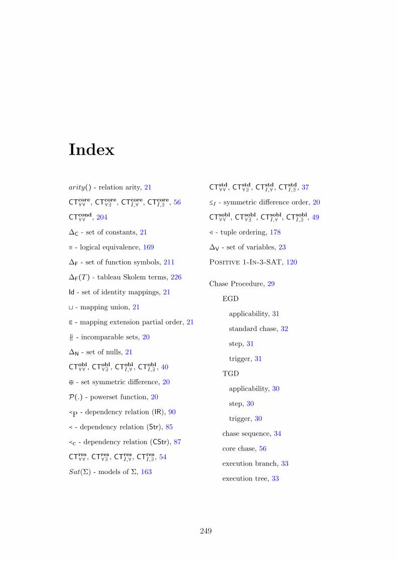
Index
arity() - relation arity, 21
CTcore∀∀ , CTcore
∀∃ , CTcoreI,∀ , CTcore
I,∃ , 56
CTcond∀∀ , 204
ΔC - set of constants, 21
≡ - logical equivalence, 169
ΔF - set of function symbols, 211
ΔF(T ) - tableau Skolem terms, 226
Id - set of identity mappings, 21
⊔ - mapping union, 21
⋐ - mapping extension partial order, 21
∦ - incomparable sets, 20
ΔN - set of nulls, 21
CTobl∀∀ , CTobl
∀∃ , CToblI,∀ , CTobl
I,∃ , 40
⊕ - set symmetric difference, 20
P(.) - powerset function, 20
≺P - dependency relation (IR), 90
≺ - dependency relation (Str), 85
≺c - dependency relation (CStr), 87
CTres∀∀ , CTres
∀∃ , CTresI,∀, CTres
I,∃ , 54
Sat(Σ) - models of Σ, 163
CTstd∀∀ , CTstd
∀∃ , CTstdI,∀ , CTstd
I,∃ , 37
≤I - symmetric difference order, 20
CTsobl∀∀ , CTsobl
∀∃ , CTsoblI,∀ , CTsobl
I,∃ , 49
⋖ - tuple ordering, 178
ΔV - set of variables, 23
Positive 1-In-3-SAT, 120
Chase Procedure, 29
EGD
applicability, 31
standard chase, 32
step, 31
trigger, 31
TGD
applicability, 30
step, 30
trigger, 30
chase sequence, 34
core chase, 56
execution branch, 33
execution tree, 33
249
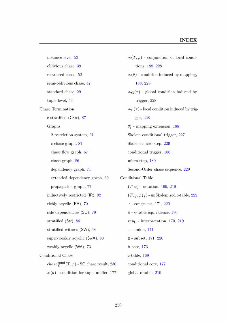
INDEX
instance level, 53
oblivious chase, 39
restricted chase, 52
semi-oblivious chase, 47
standard chase, 29
tuple level, 53
Chase Termination
c-stratified (CStr), 87
Graphs
2-restriction system, 91
c-chase graph, 87
chase flow graph, 67
chase graph, 86
dependency graph, 71
extended dependency graph, 69
propagation graph, 77
inductively restricted (IR), 92
richly acyclic (RA), 70
safe dependencies (SD), 79
stratified (Str), 86
stratified-witness (SW), 68
super-weakly acyclic (SwA), 83
weakly acyclic (WA), 73
Conditional Chase
chasecondΣ (T,ϕ) - SO chase result, 230
F(θ) - condition for tuple unifier, 177
⩕(T,ϕ) - conjunction of local condi-
tions, 188, 228
⩕(θ) - condition induced by mapping,
188, 228
⩕G(τ) - global condition induced by
trigger, 228
⩕L(τ) - local condition induced by trig-
ger, 228
θτ1 - mapping extension, 188
Skolem conditional trigger, 227
Skolem micro-step, 229
conditional trigger, 186
micro-step, 189
Second-Order chase sequence, 229
Conditional Table
(T,ϕ) - notation, 169, 219
(T ↓f , ϕ↓f) - unSkolemized c-table, 222
≅ - congruent, 171, 220
≡ - c-table equivalence, 170
repC - interpretation, 170, 219
⊔ - union, 171
⊑ - subset, 171, 220
h-core, 173
c-table, 169
conditional core, 177
global c-table, 219
250

INDEX
global condition, 219
local condition, 169
satisfiability, 171
Data Correspondence
existence-of-solution problem, 134
solution-checking problem, 134
data correspondence TGD, 129
data correspondence mapping, 130
non-uniform ⊕-solution, 131
non-uniform correspondence, 131
non-uniform subset-solution, 131
non-uniform superset-solution, 131
uniform ⊕-solution, 130
uniform correspondence, 130
uniform correspondence problem, 130
uniform subset-solution, 130
uniform superset-solution, 130
Data Exchange, 105
certainM(q, I) - certain answer set, 107
SolM(I) - solution set, 106
certain answer, 107
core solution, 110
mapping, 106
solution, 106
Data Repair, 112
⊕-solution, 113
existence-of-repair problem, 114
repair-checking problem, 114
solution, 113
subset-solution, 113
superset-solution, 113
Database
null-pos(., .) - null positions, 90
fact, 21
infinite instance, 21
instance, 21
position, 67
schema, 21
tuple, 20
Dependency, 26
aff-cl(., .) - affected position (IR), 91
aff(.) - affected position (SD), 77
∣ Σ ∣ - size for st-SO dependencies, 212
pos(.) - all positions in Σ, 91
rank(.) - position rank, 121
EGD, 26
GTGD - guarded TGD, 110
LAV, 27
st-SO dependencies , 209
TGD, 26
TGD(.) - class restriction, 28
disjoining, 205
251

INDEX
enrichment, 45
semi-enrichment, 50
TGD∨, 27
TGD∨,≠, 63
TGD∨,¬, 27
TGD¬, 27
LAV∗, 27
WGTGD - weakly guarded TGD, 110
atom position, 80
body, 26
embedded dependencies, 26
falsehood, 63
full TGD, 27
guard, 110
head, 26
model, 102
place, 80
semi-LAV, 122
source-to-target TGD’s, 28
strong universal model, 103
term, 208
universal model, 103
unsafe position, 122
weak universal model, 103
Homomorphism, 22
D-retraction, 172
Σ-satisfying homomorphism, 115
embedding, 22
endomorphism, 23
extension, 23
full homomorphism, 22
isomorphism, 23
retraction, 23
Incomplete Database, 25
certain answer, 25
possible answer, 25
possible worlds, 25
Instance
ΔC(I) - instance constants, 22
dom(I) - active domain, 22
E - equality relation, 212
Inst∗(R) - ground instances, 22
Inst(R) - set of instances, 22
I ∣R - restricted instance, 22
ΔN(I) - instance nulls, 22
block, 117
blocksize, 117
bounded block size, 118
core, 23
Gaifman graph, 117
Gaifman graph of nulls, 117
ground instance, 22
252

INDEX
incomplete instance, 22
proper retract, 23
retract, 23
Skolem instance, 211
tableau, 22, 169
tuple mgu (mgu(t1, t2)), 177
tuple unifiable, 176
tuple unifier, 176
unifier, 173, 226
isomorphic, 174
more general unifier, 173, 226
most general unifier (mgu), 174, 226
valuation, 25
Query
atom, 23
boolean query, 24
CQ, 23
exact answer, 25
naıve evaluation, 109
UCQ, 24
Semantics
SolCWAM (I) - CWA sol. space, 154
SolGCWA∗
M (I) - GCWA sol. space, 159
SolGCWAM (I) - GCWA sol. space, 155
SolPWSM (I) - PWS sol. space, 156
⊆min (M,I), 155
Constructible Models, 160
Σ(I) - set of const. models, 163
C(I,G), 163, 214
SolCMM(I), 164, 217, 219
chase sequence, 162, 213
chase sequence limit, 163, 213
chase tree, 161
constructible models, 163, 214
failing sequence, 213
ground TGD’s, 162
CWA, 154
CWA - solutions, 158
GCWA, 155
GCWA∗, 159
PWS, 156
Strong Data Exchange System, 235
fullTGDCM , 236
GCOND - class of global conditional
tables, 220
ordSO, 237
TGDCM , 236
Strong Representation Systems, 234
COND - class of conditional tables, 234
I - class of general instances, 234
G - class of ground instances, 234
253