The Charles Stark Draper Laboratory, Inc. - ntrs.nasa.gov · PDF fileAND CONTROL OF AN...

P

,,',..;,#.5.,,'/d Z - ," s s s _/ ,_"

CSDL-T-1036

GUIDANCE, STEERING, LOAD RELIEFAND CONTROL OF AN

ASYMMETRIC LAUNCH VEHICLE

by

Frederick W. Boelitz

August 1989

Master of Science Thesis

Massachusetts Institute of Technology

The Charles Stark Draper Laboratory, Inc.555 Technology SquareCambridge, Massachusetts 02139

t', C _ _r •, _,i_. :r, t tJ

https://ntrs.nasa.gov/search.jsp?R=19900004941 2018-05-13T12:21:10+00:00Z

GUIDANCE, STEERING, LOAD RELIEFAND CONTROL OF AN

ASYMMETRIC LAUNCH VEHICLE

Frederick

B.S.M.E., University

by

W. Boelitz

of Massachusetts, (1986)

Submitted in Partial Fulfillment

of the Requirements for theDegree of

MASTER OF SCIENCE

at the

MASSACHUSETTS INSTITUTE OF TECHNOLOGY

Signature of Author

September 1989

© Frederick W. Boelitz, 1989

_ I ieptemberDepartmen_gine%r_g_

Certified by

Approved

Professor

Thesis Advisor, Department of

by_

William K. Durfee

Mechanical Engineering

Gilbert S. Stubbs

CSDL Project Manager

Accepted byAin A. Sonin

Chairman, Department Graduate Committee

Guidance, Steering, Load Relief and Control

of an Asymmetric Launch Vehicle

by

Frederick Wall Boelitz

Submitted to the Department of Mechanical Engineering

in partial fulfillment of the requirements for the

Degree of Master of Science

Abstract

A new guidance, steering, and control concept is described andevaluated for the Third Phase of an asymmetrical configuration of the AdvancedLaunch System (ALS). The study also includes the consideration of trajectoryshaping issues and trajectory design as well as the development of angularrate, angular acceleration, angle of attack, and dynamic pressure estimators.

The Third Phase guidance, steering and control system is based oncontrolling the acceleration-direction of the vehicle after an initial launchmaneuver. Unlike traditional concepts the alignment of the estimated andcommanded acceleration-directions is unimpaired by an add-on load relief.Instead, the acceleration-direction steering-control system features a controloverride that limits the product of estimated dynamic pressure and estimatedangle of attack. When this product is not being limited, control is basedexclusively on the commanded acceleration-direction without load relief.During limiting, control is based on nulling the error between the limited angleof attack and the estimated angle of attack. This limiting feature provides fullfreedom to the acceleration-direction steering and control to shape thetrajectory within the limit, and also gives full priority to the limiting of angle ofattack when necessary.

The flight software concepts were analyzed on the basis of their effectson pitch plane motion. The stability of both the acceleration-direction controlmode and the angle of attack control mode was also evaluated. Simulationstudies were conducted to evaluate the performance of all the estimators aswell as the Phase Three steering, guidance and control concept. Results of thestudy indicate that the system can effectively steer to the desired trajectory aswell as provide fast load relief response.

2

Acknowledgement

This report was prepared by The Charles Stark Draper Laboratory, Inc.

under Task Order 74 from the National Space and Aeronautics Administration

Langley Research Center under Contract NAS9-18147 with the National Space

and Aerona_Jtics Administration Johnson Space Center.

While working on my Masters Thesis I received help and advice from

many people. I would especially like to thank Mr. Gilbert Stubbs, and Mr.

Richard Goss for their many hours of assistance. With their help, they made the

task of completing my thesis both enjoyable and challenging. I would also like

to thank Jeannie Sullivan who spent many hours helping me with the

acceleration-direction concept.

Thank you also to my friends Joe, Anthony, Steve, Carolyne, (spring

break crew - Ralph, Ronbo, and Pete), Carol, Carole, Margaret, Tony, Mike,

Dino, Kelly, Kellie, Kelleye, Jesse, Bob P., Dave, Duncan, and Bob R.

Without all of you, it would have been HELL.

Finally, I would like to thank my family for all their love and

encouragement over the years. This thesis is dedicated to you.

Publication of this report does not constitute approval by the Draper

Laboratory or the sponsoring agency of the findings or conclusions contained

herein. It is published for the exchange and stimulation of ideas.

I hereby assign my copyright of this thesis to the Charles Stark Draper

Laboratory, Inc., Cambridge, Massachusetts.

Permission is hereby granted by the Charles Stark Draper Laboratory,

Inc. to the Massachusetts Institute of Technology to reproduce any or all of this

thesis.

3

Table of Contents

Chapter Page

1. Introduction ..................................................................................................... 17

1.1 Background ............................................................................................. 17

1.2 Overview .................................................................................................. 17

2. Description of the Vehicle and its Flight Phases .......................... 22

2.1 Physical Configuration of the ALS Vehicle ....................................... 22

2.2 Flight Phases .......................................................................................... 28

2.3 Coordinate Frames ................................................................................ 30

2.4 Constraints .............................................................................................. 32

2.5 Rigid Body Motion .................................................................................. 36

2.6 Aerodynamic Characteristics ............................................................... 39

2.7 Mass Properties ..................................................................................... 39

3. Acceleration-Direction Guidance, Steering, and Control ......... 42

3.1 Introduction ............................................................................................. 42

3.2 Estimators for the ALS .......................................................................... 50

3.3 Acceleration Direction Estimator ......................................................... 51

3.3.1 Introduction ............................................................................. 51

3.3.2 Calculation Procedure .......................................................... 52

3.4 Approximate Vehicle Transfer Function Relationships

for Stability Analysis ............................................................................. 55

3.5 Nozzle Command Conversion Relationship .................................... 60

3.6 Approximate Transfer Functions for the Qo_-Limit Mode ................. 64

4

Chapter Page

3.7 Approximate Transfer Functions for Acceleration-

Direction Feedback Mode .................................................................... 64

3.8 Approximate Analytical Stability

Analysis Without Sampling Effects ..................................................... 68

3.9 Approximate Stability Analysis with Sampling Effects .................... 74

3.10 Control Gain Reset Procedure for Mode Switching ........................ 79

4. Angular Rate Estimation ........................................................................... 83

4.1 Description .............................................................................................. 83

4.2 The Complementary Filter .................................................................... 84

4.3 ALS Rate Estimation ............................................................................. 84

4.4 Digital Complementary Filter ............................................................... 88

4.5 Low Frequency Angular Rate Estimate ............................................. 91

4.6 High Frequency Angular Rate Estimate ............................................ 92

4.7 Acceleration Bias Estimate .................................................................. 98

4.8 Frequency Response and Transient Response ............................. 100

4.8.1 General .................................................................................. 100

4.8.2 Estimator Transfer Functions ............................................. 102

4.8.3 Rate Estimator Coefficients ................................................ 104

4.8.4 Frequency Response Characteristics .............................. 105

4.8.5 Quantization Effects ............................................................ 107

4.8.6 Simulation Results .............................................................. 112

5. Angle of Attack Estimation ..................................................................... 118

5.1 Introduction ........................................................................................... 118

5.2 The Complementary Filter .................................................................. 120

5.3 The Digital Complementary Filter ..................................................... 120

Chapter Page

So

a

5.4 High Frequency Angle of Attack Estimate ....................................... 122

5.5 Low Frequency Angle of Attack Estimate ........................................ 126

5.6 Angle of Attack Filter Coefficients ..................................................... 130

5.6.1 Issues Effecting Choice of Filter Coefficients ................. 130

Dynamic Pressure Estimation .............................................................. 135

6.1 Introduction ........................................................................................... 135

6.2 Estimation Procedure .......................................................................... 136

6.3 Effects of Improved Air-Relative Velocity Estimation ..................... 140

Trajectory Design ....................................................................................... 143

7.1 Introduction ........................................................................................... 143

7.2 Phase Two Functionalization ............................................................ 146

7.3 Phase Three Functionalization ......................................................... 148

7.4 Predictive-Adaptive Guidance for Phase Four ............................... 150

7.5 Trajectory Parameter Sensitivity Analysis ....................................... 151

7.5.1 Sensitivity Analysis Plots ................................................... 153

7.6 Effects of Winds on Trajectory Design ............................................. 162

7.7 Stored Acceleration-Direction ........................................................... 164

7.8 Launch Maneuver Design .................................................................. 165

7.8.1

7.8.2

7.8.3

7.8.4

General Description ............................................................ 165

Launch Maneuver Simulation ........................................... 166

Launch Maneuver Correlation Results ............................ 170

Sinusoidal Launch Maneuver Parameter

Adjustment ............................................................................ 173

6

Chapter Page

m

.

7.8.5 Parameter Adjustment for the Sinusoidal

Launch Maneuver with a Non-Zero

Terminal Pitch rate .............................................................. 174

Simulation Results ..................................................................................... 177

8.1 Introduction ........................................................................................... 177

8.2 Discussion of Results .......................................................................... 181

Conclusions and Recommendations ................................................. 199

9.1 Conclusions .......................................................................................... 199

9.2 Recommendations ............................................................................... 201

Appendix Page

A. Derivation of Equations of Motion ...................................................... 203

B. Determination of Aero-Coefficients ................................................... 207

C. Determination of Mass Properties ...................................................... 209

D. Vehicle Rigid Body Equations of Motion ......................................... 212

E. Continuous Rate Estimator Transfer Functions ........................... 221

El Relationships Between Continuous

and Discrete Rate Estimator Coefficients ....................................... 225

G. Wind Profiles ................................................................................................ 228

List of References ............................................................................................... 231

List of Figures

Figure Page

2.1

2.2

2.3

2.4

2.5

2.6

2.7

3.1

3.4

3.5

3.6

3.7

3.8

3.9

3.10

ALS general configuration ............................................................................ 23

ALS gimballing and engine cant relationship ........................................... 25

Net acceleration direction at liftoff ................................................................ 27

ALS flight phases ............................................................................................ 29

Body frame with local geographic frame .................................................... 32

Reference frame relationships ..................................................................... 33

ALS dynamic pressure profile ...................................................................... 35

Generic block diagram defining guidance, steering,

and control operations .................................................................................. 43

Elements of the vehicle control and estimation ......................................... 45

Traditional acceleration-direction guidance with

combined steering and control loop with add-on load relief .................. 46

SSTO guidance, steering and control system

for Phase Three ............................................................................................... 48

Improved acceleration-direction guidance, steering

and control for Phase Three of the ALS, with Q_-

limit override replacing add-on load relief ................................................. 49

Approximate transfer functions for Phase One

and Two and for the Qo_-Iimit mode in Phase Three ................................ 56

Approximate transfer functions for the acceleration-

direction mode in Phase Three .................................................................... 57

Single nozzle deflection configuration ....................................................... 61

Moment generated by ALS nozzle deflections ......................................... 62

ALS nozzle command block diagram ......................................................... 63

Figure Page

3.11

3.12

3.13

3.14

4.1

4.2

4.3

4.4

4.5

4.8

4.9

4.10

4.11

4.12

4.13

4.14

4.15

4.16

Nichols plot for Qcz-limiting mode ................................................................ 78

Nichols plot for acceleration-direction mode ............................................. 78

Control integrator reset for control mode switching .................................. 82

Nozzle command during control integrator reset ...................................... 82

Block diagram development of complementary filter ............................... 85

Continuous ALS rate estimator .................................................................... 86

Simplified continuous ALS rate estimator .................................................. 86

Thrust vector misalignment contribution to estimated rate ...................... 87

Simplified continuous ALS rate estimator with

estimated angular acceleration feedback ................................................. 88

Digital rate estimator ...................................................................................... 90

Vehicle description for the derivation of estimated

high frequency angular rate ......................................................................... 93

Rate estimator block diagram without acceleration

bias estimation ................................................................................................ 99

Rate estimator block diagram with acceleration

bias estimation .............................................................................................. 101

Simplified continuous rate estimator design loop .................................. 103

Frequency response of o-_0 b ..................................................................... 107

Frequency response of o)2/(J_b ..................................................................... 108

Frequency response of _/_b ....................................................................... 108

True pitch rate ................................................................................................ 114

True angular acceleration ........................................................................... 114

Pitch rate with 3 arcsec and 0.0128 ft/sec quantization ......................... 115

9

Figure Page

4.17

4.18

4.19

4.20

4.21

5.1

5.2

5.3

5.4

5.5

5.6

5.7

5.8

5.9

6.1

(^)Angular acceleration _1 with 3 arcsec and 0.0128 ft/sec

quantization ................................................................................................... 11 5

(^)Angular acceleration _2 with 3 arcsec and 0.0128 _sec

quantization ................................................................................................... 1 1 6

Pitch rate with 11 arcsec and 0.0320 quantization ................................. 11 6

(^)Angular acceleration _1 with 11 arcsec and 0.032 ft/sec

quantization ................................................................................................... 1 17

(^)Angular acceleration _2 with 11 arcsec and 0.0320 II/sec

quantization ................................................................................................... 11 7

Second order complementary filter ........................................................... 120

Digital second order complementary filter ............................................... 17_1

Digital angle of attack second order complementary filter .................... 122

Vehicle orientation parameters .................................................................. 124

Typical _ profile for Phase Three ................................................................ 125

Low frequency angle of attack flow chart ................................................. 127

Vehicle free body diagram for the determination of Fn .......................... 129

Angle of attack error using (_-_2)with quantization

levels of 3 arcsec and 0.0128 ft/sec .......................................................... 134

Angle of attack error using (_-o2)with quantization levels

of 110 arcsec and 0.0128 ft/sec ................................................................. 134

Q based on earth-relative and air-relative velocities

using tail wind Vandenberg #69 wind profile .......................................... 136

Vector relationships for air-relative velocity estimator ........................... 140

Error in estimated and true air-relative velocity

magnitude for Vandenberg wind profile #70 ........................................... 142

10

Figure Page

6.4

7.1

7.2

7.5

7.6

7.7

7.8

7.9

7.10

7.11

7.12

7.13

Error in estimated and true air-relative velocity

magnitude for Vandenberg wind profile #69 ........................................... 142

Phase Two command profile with sinusoidal

pitch rate ......................................................................................................... 147

Phase Two command profile with constant

terminal pitch rate ................................................................... ...................... 148

Trajectory shaping angle of attack profile ................................................ 149

Sensitivity of gamma to Qo_ limit for a non-zero

terminal pitch rate maneuver ...................................................................... 153

Sensitivity of theta to Qo_ limit for a non-zero terminal

pitch rate maneuver ...................................................................................... 155

Sensitivity of gamma to terminal launch theta for a non-

zero terminal pitch rate maneuver ............................................................. 155

Sensitivity of theta to terminal launch theta for a non-


Sensitivity of gamma to (zl for a non-zero terminal


Sensitivity of theta to al for a non-zero terminal


Sensitivity of gamma to variations in 0_2 for a non-


Sensitivity of theta to variations in a2 for a non-


Sensitivity of gamma to variations in terminal pitch

rate for a non-zero terminal pitch rate maneuver .................................... 158

Sensitivity of theta to variations in terminal pitch

rate for a non-zero terminal pitch rate maneuver .................................... 159

11

Figure Page

7.14

7.15

7.16

7.17

7.18

7.19

7.20

7.21

7.22

7.23

7.24

7.25

7.26

7.27

8.1

Sensitivity of gamma to Qo_ limit for a sinusoidal


Sensitivity of theta to Qo_ limit for a sinusoidat


Sensitivity of gamma to e_l for a sinusoidal


Sensitivity of theta to _1 limit for a sinusoidal


Sensitivity of gamma to e_2 for a sinusoidal


Sensitivity of theta to e_2 limit for a sinusoidal


Effect of tail and head winds on the predicted

on-orbit mass ................................................................................................. 164

Commanded and filtered acceleration-direction

profile in body coordinates .......................................................................... 165

Simplified dynamic model for launch profile ........................................... 168

Sinusoidal launch maneuver correlation between

true and estimated Y..................................................................................... 1 71

Sinusoidal launch maneuver correlation between

true and estimated e_.................................................................................... 1 71

Sinusoidal launch maneuver with non-zero terminal

pitch rate: correlation between true and estimated 1'............................. 172

Sinusoidal launch maneuver with non-zero terminal

pitch rate: correlation between true and estimated e_............................. 172

Sinusoidal launch maneuver flow chart ................................................... 175

Simulation run number 1 ............................................................................. 187

12

Figure Page

8.2

8.3

8.4

8.5

8.6

8.7

8.8

8.9

8.10

8.11

8.12

8.13

8.14

8.15

8.16

8.17

8.18

8.19

8.20

8.21

8.22

8.23

Simulation run number 1............................................................................. 188

Simulation run number 1............................................................................. 188


















Simulation run number 10 .......................................................................... 197



13

Figure Page

B.1

C.1

C.2

D.1

F.1

G.1

G.2

Determination of Cn by linear interpolation ............................................. 207

Booster stage component masses and dimensions .............................. 209

Core stage component masses and dimensions ................................... 210

Vehicle Free Body Diagram ........................................................................ 213

Unmodeled angular acceleration estimator loop ................................... 226

Vandenberg #69 and #70 wind profiles ................................................... 229

Linearized Vandenberg #69 and #70 wind profiles ............................... 230

14

List of Tables

Table Page

2.1

2.2

3.1

3.4

4.1

4.2

4.3

4.4

5.1

5.2

7.1

7.2

ALS engine data ............................................................................................. 24

Summary of mass properties ........................................................................ 41

Stability statistics for Q_-Iimit mode

at different critical times in the trajectory .................................................... 76

Selected gains for Qcc limiting mode ........................................................... 76

Stability statistics for acceleration-direction mode

at different critical times in the trajectory ..................................................... 77

Selected gains for acceleration-direction

steering mode .................................................................................................. 77

Continuous and discrete rate filter constants .......................................... 106

Effects of quantization on error in estimated pitch rate .......................... 112

Effects of quantization on error in estimated

angular acceleration using (_1) .................................................................. 113

Effects of quantization on error in estimated

angular acceleration using (_2) .................................................................. 113

(^)Effects of quantization in angle of attack error using _1 ...................... 133

(^)Effects of quantization in angle of attack error using _2 ...................... 133

Trajectory shaping results ........................................................................... 154

Effects of winds on trajectory parameters and

on-orbit mass ................................................................................................. 163

Peak errors in launch design simulations ................................................ 170

Simulation results for acceleration-direction concept

with perfect feedback quantities ................................................................. 179

15

Table Page

8.2

8.3

8.4

8.5

B.1

C.1

D.1

Maximum Q and Q(z values for acceleration-

direction concept simulations ..................................................................... 180

Simulation results for acceleration-direction

concept using estimated angle of attack, angular

rate, and dynamic pressure ....................................................................... 180

Maximum Q and Q_ values for acceleration-direction

concept simulations using estimated feedback variables ..................... 1 81

Effects of estimators and quantization on

performance of run #1 .................................................................................. 185

Procedure for determining Cn .................................................................... 208

Core and booster propulsion module masses ........................................ 211

Typical rigid body dynamic coefficients .................................................... 219

16

Chapter One

INTRODUCTION

1.1 Background

This thesis will analyze and evaluate guidance, steering and control

concepts for one configuration of an early design of the Advanced Launch

System (ALS) being developed by NASA and the US Air Force. The basic

launch vehicle design that will be employed in this investigation was proposed

by General Dynamics in 1988. The vehicle consists of a 293 ft. long core stage

which can have either one or two booster stages of roughly half its length

attached in a parallel configuration with the engine nozzles of the core and

booster stages at the same longitudinal station. If two booster stages are

employed they are attached to the core at diametrically opposite locations so as

to achieve symmetry. The single attached booster stage produces an

unavoidable asymmetry that must be addressed in the design of the guidance,

steering and controls. Both the core and booster stages employ liquid oxygen

(LOX) and liquid hydrogen (LH) for propulsion, employing low-cost, non-

throttleable engines.

Since the guidance, steering and control problems are most severe for

the case of the asymmetrical launch vehicle employing only one booster stage it

was decided to use this vehicle configuration as the basis for analysis and

evaluation. The flight concepts developed for this configuration should then be

applicable to the symmetric configuration employing two booster stages.

1.2 Overview

The guidance, steering, and control system studied for the ALS builds

upon the concepts studied previously by Corvin for the single stage to orbit

(SSTO) Shuttle II, with some important modifications, additions and innovations.

17

Both the SSTO and ALS systems were designed to achieve close to an all-

weather launch capability and a greater autonomy then is currently possible

with the Space Shuttle and many unmanned launch vehicles. The ALS system

is similar to the SSTO system in its prelaunch trajectory design and its use of

prelaunch doppler radar wind measurements to optimize the atmospheric

phases of the boost trajectory. In both systems there are four distinct phases:

(1)

(2)

(3)

(4)

Phase One, in which the vehicle rises nearly vertically to clear the

launch tower.

Phase Two, in which the vehicle is pitched over rapidly. (in

accordance with prelaunch computations)

Phase Three, in which the vehicle is pitched over more slowly.

(again in accordance with prelaunch computations, but subject to

a load relief constraint on the estimated angle of attack)

Phase Four, in which a predictive-adaptive Powered Explicit

Guidance (now employed in the Space Shuttle) determines the

direction of the vehicle acceleration in the upper atmosphere and

beyond.

The ALS system studied in this thesis differs from the SSTO system

studied by Corvin in two important respects. First, in the development of a

completely different implementation of Phase Three, and second in the

development of control signal estimators that deal with the problems resulting

from asymmetry in the ALS vehicle. In addition, an optional implementation of

Phase Two was studied. The new features are summarized below:

(1) An optional functionalization of commanded attitude versus time in

Phase Two that is designed to achieve a specified angular rate in addition to a

specified attitude and angle of attack at the beginning of Phase Three.

(2) The replacement in Phase Three of the SSTO combination of

velocity direction steering and angle of attack control with an alternative concept

18

of an acceleration-direction steering-control system with a control overridefeature that limits the product of estimated dynamic pressure and estimatedangle of attack.

(3) The modification of the prelaunch trajectory design program togenerate and store (for in-flight use) the acceleration direction instead of thevelocity direction as in the SSTO system.

(4) An angular rate estimator that employs a first order complementary

filter to combine (a) a low frequency rate estimate based on measured attitude

increments and (b) a high frequency rate estimate based on estimated angular

acceleration.

(5) An angular acceleration estimator (for use in the angular rate

estimator and angle of attack estimator) that utilizes accelerometer measured

velocity increments in combination with measured deflections of all the engines

to determine an angular acceleration estimate that is corrected for mismodeling

of the magnitudes and points of application of forces acting on the vehicle.

(6) A correction feedback loop in the angular acceleration estimator

that computes an acceleration correction signal from the integral of the filtered

difference between the estimated angular acceleration and the angular

acceleration computed from the back difference of estimated angular rate.

(7) An angle of attack estimator employing a second order

complementary filter to combine (a) a low frequency angle of attack estimate

based on accelerometer measured velocity increments, measured engine

deflections, estimated angular acceleration and estimated dynamic pressure

and (b) a high frequency angle of attack estimate based on measured attitude.

(8) A dynamic pressure estimator (for use in the angle of attack

estimator) that computes the air density from the estimated altitude and that

19

utilizes estimated values of earth-relative velocity and angle of attack to

estimate the air-relative velocity.

In order to limit the scope of this thesis investigation to a level consistent

with the availability of design data and the constraints of time it was decided to

describe and evaluate the flight software concepts in terms of pitch plane

problems, assuming no yaw or roll motion of the vehicle. Except for the

possibility of commanding a zero yaw angle of attack to minimize undesirable

aerodynamic torques about the roll axis resulting from vehicle asymmetry, the

flight software concepts outlined above should be applicable also to yaw-axis

guidance, steering and control.

The flight software concepts will be analyzed and evaluated for their

effects on pitch-plane motion first in terms of frequency response characteristics

where appropriate and second in terms of transient response characteristics.

Since bending and sloshing characteristics have yet to be determined for

the ALS design, the vehicle characteristics will be approximated by a rigid body

model.

The transient response evaluations will be based on two Jimsphere-

measured wind profiles representing the worst-case variations in the winds over

a 3 and 1/2 hour period. The first wind profile will be employed in the prelaunch

trajectory design program to determine post launch profiles for commanded

attitude and commanded specific force direction. The effects of changes in the

winds between the prelaunch trajectory design computations and the

subsequent in-flight utilization of these computations will be represented by

using the second wind profile for flight simulation.

In both the trajectory design computations and the flight simulation it will

be assumed that the Powered Explicit Guidance (PEG) developed for the

Space Shuttle takes over some time before the point of booster separation.

This guidance technique generates a specific force direction versus time profile

that is close to optimal, assuming that aerodynamic forces can be neglected.

Subsequent to booster stage separation, an analytical prediction performed by

PEG is employed to approximately determine the on-orbit mass that will result

from the vehicle state achieved at booster separation.

20

This thesis study of ALS software concepts is a prelude to a follow-on

study that will employ a more comprehensive model of the launch vehicle

(including slosh and bending modes) and will investigate the use of predictive

adaptive techniques to enhance performance. Conclusions and

recommendations of this thesis will relate to the subsequent follow-on

investigation.

21

Chapter Two

DESCRIRTION OF THE VEHICLE AND ITSFLIGHT PHASES

2.1 Physical Configuration of the A.L.S. Vehicle

Figure 2.1 illustrates the minimum-payload asymmetrical configuration of

the Advanced Launch System for which the guidance, steering and control

concepts will be developed and evaluated in this thesis. As shown in this

figure, this configuration consists of a core stage with a single attached booster

stage. Both core and booster stages have identical non-throttleable engines

employing liquid hydrogen (LH) and liquid oxygen (LOX), with a thrust level of

612,000 Ibs per engine. These stages also have identical LH and LOX tanks.

The larger number of engines of the booster results in its propellant tanks being

drained before those of the core stage. When the booster fuel tanks have been

expended the booster stage is separated from the core. Figure 2.1 also shows

the following differences between the core and booster stages:

(i)

(2)

(3)

(4)

The core stage has a length of 293 ft, compared to the booster

length of 161 ft.

The upper portion of the core contains the payload bay. The

diameter of the payload bay is larger than the diameter of the

lower portion of the core, whose diameter equals that of the

booster.

The inertial measurement unit (IMU) is located in the lower portion

of the core below the LH tank.

All seven booster engines, their servos, and their fuel distribution

lines are housed in a Booster Recovery Module (BRM).

Separation of the BRM occurs approximately twenty seconds after

22

Core

Length

Booster

Length

Gross

Liftoff

Weight

DryWeight

293 ft.

161 ft.

3,782,000 Ibs.

331,0001bs.

- Payload Bay

Booster RecoveryModule

Liquid Oxygen Tank

Inter-Tank Adapter

Liquid Hydrogen tank

IMU

7 LH/LOX Engines ---- -- 3 LH/LOX Engines

Figure 2.1 A.L.S. General Configuration

23

(5)

core/booster separation and parachutes are used to return the

module to Earth. Recovery of the BRM is made at sea. The

remaining components of the booster and core stages are not

reusable.

The ALS vehicle employs 10 gas generator fixed thrust engines.

All of the engines are of the same type and all possess pitch and

yaw plane gimballing capability. Table 2.1 is a summary of the

physical characteristics of the engines. The vacuum thrust, the

propellent flow rate, the cross section area of the engine, and the

local atmospheric pressure are used to calculate the thrust

generated by the vehicle. In addition because of the asymmetry of

the vehicle all engines are installed with a 5 ° cant as illustrated in

Figure 2.2. This provides the vehicle with a wider gimballing

margin to help withstand "engine out" possibilities and large

wind/gust dispersions.

NAME

Cycle

SPECIFICATION

Gas Generator

Propellants LOX/LH

Throttling Rage Fixed

Propellant Flow Rate 1,427 Lbs/sec

Vacuum Thrust 612 KLbs

Weight 6,744 Lbs

Inside Diameter 88.0 in

Length

Table 2.1 ALS engine data.

150 in

The exact location of all ten core and booster engines, and the

manner in which individual engine deflections are to be

commanded to produce desired attitude changes were not

24

specified in the design data package employed in this thesis.

Therefore, to simplify the analysis it was decided to assume that

the vehicle is controlled by two resultant thrust vectors, one for the

core engines and one for the booster engines. Both resultant

thrust vectors are assumed to be deflected by the same pitch

angle, 8, which is computed by the flight control system. The

deflection of the two engine thrust vectors can then cause torques

on the vehicle which cause it to rotate to its commanded inertial

attitude.

Booster,7 Engines

B

Install

9o9o

Core,3 Engines

5°

Gimballing capability:1:9° from installed cant

NOTE

1) All 10 engines are installed with a 5 ° cant.2) All 10 engines have the same gimballing capability.3) Resultant thrust vector of core acts through point A.4) Resultant thrust vector of booster acts through point B.

Figure 2.2 ALS gimballing and engine cant relationship.

25

At this point it is appropriate to mention that the asymmetry in the launch

vehicle of Figure 2.1 has made it necessary to employ the following operational

modes and software design features:

(I)

(2)

(3)

In order to minimize the aerodynamic roll torques, which are

magnified by the asymmetry, it was decided to assume a roll

orientation that puts the booster stage on top as the vehicle

pitches over after liftoff. This orientation makes it possible to null

aerodynamic roll torques by nulling the yaw angle of attack.

As a result of vehicle asymmetry it is necessary to allow for

appreciable pitch angle of attack values throughout the trajectory,

even in the absence of winds. This is because the unequal total

thrusts of the booster and core stages make it necessary to deflect

the thrust vectors to maintain a near zero pitch rate. This is best

illustrated at liftoff where the vehicle is commanded to maintain a

90 ° pitch attitude. At ignition, the thrust deflections produce an

appreciable component of velocity perpendicular to the vehicle's

longitudinal axis, with an accompanying no-wind angle of attack in

the pitch plane. This is shown in Figure 2.3 where FTot= I

represents the effective sum of the core and booster thrusts for the

zero torque condition necessary to maintain the initial 90 ° attitude.

Also shown is the net acceleration applied to the vehicle by the

thrust and gravity forces. It can be seen from the figure that the net

acceleration vector is at an angle ¢ with respect to the vertical. As

a result, velocity is immediately developed in this direction and the

vehicle acquires an instantaneous angle of attack equal to ¢.

Although the aerodynamic pitch moment associated with the angle

of attack allows some diminishment of the pitch deflections of the

engines, these deflections must never the less be appreciable

throughout the endoatmospheric boost phase.

Although no data on the center of pressure position as a function

of Mach number and angle of attack was available for this thesis

study, it is assumed that there may be greater uncertainties in this

position as well as in the aerodynamic force magnitudes for the

26

/

Thrust Booster4

6

6

Thrust Core

Acceleration Vector Diagram at Liftoff

EarthRelativeVertical

8 A: FT°tal_'otal

//Net Instantaneous

Acceleration at Liftoff

Earth relative horizontal

i •

Figure 2.3 Net Acceleration Direction at Liftoff

27

asymmetrical vehicle. It is assumed that these uncertainties as

well as uncertainties in the thrust-produced moments may require

a special software feature that estimates the effects of torque

mismodelling in order to obtain accurate estimates of angular

acceleration, angular velocity and angle of attack for pitch plane

control.

2.2 Flight Phases

As shown in Figure 2.4 the ascent profile of the ALS consists of four

distinct flight phases which employ different guidance and control modes. The

first three of these phases are endoatmospheric. The transition to

exoatmospheric flight occurs in the last phase.

It will be noted that these phases are defined corresponding to guidance

and control modes rather than the utilization of vehicle stages. The only staging

event is the thrust termination and separation of the booster which occurs

during Phase Four.

Phase One is characterized by a near vertical rise so that the vehicle may

safely clear the launch tower. During this phase the vehicle is commanded to

maintain a 90 ° pitch attitude. Termination of Phase One and transition to Phase

Two occurs once the vehicle has reached a height of 400 ft. The next two

endoatmospheric flight phases are designed to avoid excessive loads

associated with the normal aerodynamic force. Since the magnitude of this

force is proportional to the product of the dynamic pressure, Q, times the angle

of attack, _, it is customary to constrain the atmospheric boost trajectory to avoid

a specified maximum Qo_. The manner in which this avoidance is carried out

has a crucial bearing on the safety and performance of the vehicle in its

endoatmospheric boost phases.

Once the launch tower has been cleared in Phase One, Phase Two is

initiated. This second phase covers a time period in which the value of the Q

has not risen to a value where the Qo_ limit will significantly constrain attitude

control. During this period the vehicle is maneuvered rapidly to achieve an end

state that is compatible with the initial requirements of Phase Three. The

28

0_B_ Separation

_/ T _=180 sec. -,-,-,--

v Booster separatedfrom CoreT _=160 sec.

Phase Four

• Exoatmospheric Flight Phase• Predictive-adaptive Powered

ExplicitGuidance (PEG)T -- 120 sec.

Maximum Q aPhase Three

• Constrained endoatmosphericflightphase

• Acceleration-direction steering,guidance, and control, subject toaQ (x limit.

A

T = 30 - 40 sec.

Phase Two

• Relatively unconstrainedrapid launch maneuver

• Attitude control unimpairedby Q a constraint.

T = 8 sec.

Phase One• Vertical rise to clear tower• Attitude control

Figure 2.4 ALS Flight Phases.

29

commanded attitude in Phase Two is generated by an analytical function of timewhose parameters are determined prior to launch by a trajectory design

program described in Chapter Seven.

Phase Three covers a time period in which Q is sufficiently high that thelimit on the Qcxproduct can significantly constrain the boost trajectory. During

this phase the vehicle's acceleration direction is controlled subject to the Qo_

limit. The commanded acceleration direction in Phase Three is obtained from a

stored time profile generated prior to launch by the trajectory design program.

Phase Four is defined to begin at the point where the guidance shifts

from one of the alternatives in Phase Three to a predictive-adaptive guidance

method known as Powered Explicit Guidance (PEG). This method analytically

predicts the on-orbit mass in cut-and-try computations which neglect the effects

of atmospheric drag. The differing thrust levels before and after staging are

taken into account in these computations. The direction of the thrust in each

cut-and-try prediction is based on a "linear-tangent guidance law" which then

generates the commanded thrust direction for 4 second time intervals between

PEG updates.

When PEG takes over at 120 seconds the simulation is simplified by

assuming that the thrust is in the commanded direction, with the effects of

aerodynamic drag being subtracted from the thrust produced acceleration. The

simplified simulation is terminated at the point of booster separation which

occurs out of the atmosphere at 160 seconds. At this point the PEG prediction

based on no atmosphere provides an accurate prediction of the on-orbit mass.

2.3 Coordinate Frames

To simulate and study the translational and rotational motion of the

vehicle during flight four reference frames are defined. They are :

(I) Inertial Earth Centered Reference Frame - (X, Y, Z).

All equations of motion are referred to this non-rotating Earth fixed

reference frame. The origin of the frame is at the center of the

30

Earth with the Z axis pointed through the North Pole. The positive

X axis points through 0 longitude at t=0. The ¥ direction forms a

right handed set with X and Z.

(2) Local Geographic Frame - (NORTH, EAST, UZG).

The origin of this axis is located at the cg of the vehicle. UZG

points toward the center of the Earth. NORTH lies on the plane

formed by the Z axis and I.IZG. and points toward the North Pole.

EAST completes right handed frame.

(3) Body Fixed Frame - (UBX, UBY, UBZ).

This frame is fixed to the cg of the vehicle. The U BX (roll)

coordinate points along the center line of the vehicle. The UBY

(pitch) coordinate remains perpendicular to pitch plane. U BZ

completes the right handed set.

(4) Velocity Direction Frame - (UVX, UVY, UVZ).

This frame is fixed to the cg of the vehicle. UVX is directed along

the Earth relative velocity vector. UVY is in the direction of the

cross product of the gravity vector and UVX. UVZ completes the

right handed set.

Figure 2.5 illustrates the relationship between the body axes and the

local geographic coordinate system. The attitude, heading and bank of the

vehicle is defined relative to the Local Geographic coordinate frame and the

body frame. The attitude is the only variable of interest since this study is limited

to the pitch plane. The bank of the vehicle is set to zero and the heading is

determined by the initial launch azimuth. Figure 2.6 shows the relationship

between the pitch plane trajectory of the vehicle and its inertial, body, and

velocity frames. In relation to the body frame the velocity vector is described by

two angles: the angle of attack, o_, and the sideslip angle, _. However, for this

31

study the vehicle is constrained to fly in the trajectory plane assuming zerocrosswinds, so that I_=0.

UBXroll

NORTH EAST

UBZyaw

UZG

Earth Relative Horizontal

UBYpitch

Figure 2.5 Body Frame with Local Geographic Frame

2.4 Constraints

The primary constraint on maneuvering within the atmosphere is the limit

on aerodynamic loads which are produced by the normal aerodynamic force,

F n. This force is perpendicular to the centerline of the vehicle and acts at the

32

IVY

IVX

UBX

Z

North Pole

::::::::::::::::::::::::::::::::::::::::::

X (Longitude = 0 at time = O)

Figure 2.6 Reference Frame Relationships.

33

center of pressure. As the vehicle accelerates through the atmosphere the

aerodynamic force can cause very large bending moments capable of

destroying the vehicle. For a vehicle traveling with an air relative velocity V a,

the aerodynamic normal force can be expressed as:

Fn = 21-p V 2 S Cn (2.1)

where

p = the air density

S = the cross-sectional area of the vehicle

C n = the aerodynamic normal force coefficient.

The aerodynamic normal force coefficient is a function of Mach number

and angle of attack. A simplified aerodynamic model for the the ALS was used

based on a linear relationship between Cn and ¢ for a wide range of Mach

numbers. Given this linear relationship Equation (2.1) is then expressed as

Fn = 1 p Va2 S Cna a (2.2)

where

The dynamic pressure Q, is defined as

Q = 2J-P V2 (2.3)

34

so that the above equation for normal aerodynamic force can be rewritten as

Fn -=-S Q CnQ,o_ (2.4)

To control the normal aerodynamic force, a limit is usually imposed on

the product of Q and o_. The magnitude of Q is a function of the magnitude of the

air-relative velocity of the vehicle, V a, which increases during flight, and the air

density, p, which decreases with altitude. The combined effects of the variations

in p and V a typically cause Q to maximize midway through Phase Three. In this

region of maximum Q, the aerodynamic normal force is most sensitive to

variations in angle of attack. A typical dynamic pressure profile for the ALS is

illustrated in Figure 2.7.

,1¢

.IDm

G)t._

L_

a.

om

ECO¢,.

C3

800700 t

600 t

500 t

400 t

300 t

200 1

1°i! , , , , . , , ,0 20 40 60 80 100 120 140 160

Time (sec)

Figure 2.7 ALS Dynamic Pressure Profile.

35

2.5 Rigid Body Motion

All the steering, guidance and control concepts studied in this thesis are

limited to the pitch plane and all roll and yaw motion is assumed to be zero.

As mentioned in the introduction, in the absence of bending and slosh

data for this particular ALS design it was decided to employ only a rigid body

model of the vehicle in this investigation. The equation of motion for linear

acceleration is given by the relationship:

F = m A ci (2.5)

where

F = the vector sum of all forces acting on the vehicle.

m = the total vehicle mass.

ciA = is the acceleration of the vehicle center of gravity with respect to an

inertial frame of reference.

The rotational equation of motion is given by the relationship

M = H (2.6)

where

M = the vector sum of all moments applied to the system

about the center of gravity.

and

H = the centroidal angular momentum vector.

36

The angular momentum vector is defined by the relationship

H = Io (2.7)

where

I = Inertia matrix about the center of gravity.

co = The angular rate vector of the vehicle with respect to

the inertially fixed Earth Centered Reference Frame.

For the purposes of computing the derivative of H in Equation (2.6), it is

convenient to compute the components of the inertia tensor and the

components of the angular rate vector with respect to the vehicle axis system

(u ,, u2, u3) (the body roll, pitch, and yaw axes respectively). In this system,

11 t 112 Ii 3

I21 I22 I23

I31 I32 I33

(2.8)

and

I°'lco= o2 (2.9)(O3

It is assumed in this thesis that the vehicle axis system is approximately a

principal axes set -- ie, the products of inertia are sufficiently small so that they

can be neglected. With this assumption, the angular momentum vector

computed from Equations (2.7), (2.8), and (2.9) is given by

37

n

Ill _o_

122 O)2

133 m3

(2.1o)

Equation (2.6) can now be evaluated from the following relationship

M=dHdt

relative to = d H [ relative to the + 0) x H (2.1 1)an inertial d t [ body fixed framereference frame

Substituting Equations (2.9) and (2.10)into (2.11),

M

ll 161 - 0)2(03(I22 - I33)

12 262 003C01(I33 I11)

13 363 0_1¢02(Ill I22)

(2.12)

It will be noted that terms involving derivatives of I]], I22, and I33 have

not been included in the above equations. These derivatives, which are caused

by propellant expenditure, are assumed to be negligible. The components of

Equation (2.12) represent Euler's Equations of motion. These equations can be

solved for the angular accelerations @, 6)2 and 6)3 which can then be

integrated by the ALS simulation to provide angular rate and attitude

information with respect to the body frame. In vector form, the angular

accelerations can be determined by substituting Equation (2.7) into Equation

(2.11) and solving for _ to obtain

_) = I'IM I'l (o) x (I co)) (2.13)

38

Equation (2.13) can be solved for acceleration and integrated by the ALS

simulation.

2.6 Aerodynamic Characteristics

Aerodynamic data were provided to CSDL by the NASA Langley

Research Center. Lift and drag coefficients for both the subsonic (0.1 < Mach <

2.0) and supersonic (3.0 < Mach < 10) speed ranges were provided over angles

of attack of + 20 °. Subsequently this data was converted to coefficients of

normal and axial force so that all forces on the vehicle could be summed in the

body frame. Over the entire speed range interference affects between the core

and booster stages are neglected.

Because only a discrete matrix of aerodynamic data points is available

over the specified ranges of Mach number and angle of attack, a linear

interpolation scheme is used to extract the values of aero-coefficient._ between

the data points. This is achieved by first fitting all of the aero coefficients to

several third order curves by least squares fits along lines of constant Mach

number, and then linearly interpolating between two of the constant Mach

curves termed the "Low-Mach" and "High-Mach" curves for given values of o_

and Mach Number. Appendix C contains a more detailed description of this

procedure.

Since this study is limited to the pitch plane, only those aero coefficients

affecting motion in the pitch plane are generated in the simulation. Accordingly,

all lateral forces are neglected and the vehicle is subjected only to tail and head

winds.

2.7 Mass properties

In order to simulate the dynamics of the ALS vehicle an estimation of the

moment of inertia in the pitch plane and the location of the center of gravity is

required. This is achieved in a subroutine of the main program where the mass

properties of the vehicle are updated each control cycle (100 ms) by continually

39

re-evaluating the remaining masses of core and booster propellant during flight

and adjusting the cg location and inertia of the vehicle based upon these fuel

mass properties and a pre-launch dry estimate of the vehicle mass properties.

An exact description of the ALS is not available and therefore the dry estimate is

simplified by using a model based upon several basic geometric solids in

aggregate. These solids are further assumed to have masses which are

uniformity distributed. The fuel tanks, for example, are modelled as hollow

circular cylinders.

The liquid booster stage from aft to forward consists of a Booster

Recovery Module (BRM), a liquid hydrogen tank, an inter-tank adapter, a liquid

oxygen tank, and a nose cone. All of these components are modelled as hollow

cylinders with the exception of the BRM which is modelled as a solid cylinder.

In addition, the engine modules on both stages share a common structure or

frame. However, because no information is available on the gross mass of

each module, both structures are assumed to equal 15% of their respective total

engine weights. The lower half of the core stage is modelled similarly to the

booster stage, with the exception of the payload bay. Because no specific

payload configuration was available the cargo bay was simply modelled as a

solid homogeneous cylinder.

The volumes of liquid oxygen (LOX) and liquid hydrogen (LH) in both the

core and booster stages are estimated from the total propellant weight at liftoff,

and the fuel mixture ratio (FMR) of each engine. Consequently, the amounts of

LOX and LH in each vehicle are programmed to drain simultaneously upon

engine burnout. The fuel for each vehicle is modelled as a pair of solid

cylinders, one on top of the other, running lengthwise along the vehicle with the

liquid hydrogen tanks located aft. As liquid propellant is combined and then

ignited the inertia model assumes that all of the remaining fuels form

homogeneous cylinders at the base of each fuel container. Table 2.2 shows a

summary of the dry mass properties of the A.L.S. A more detailed description of

the dry inertia model can be found in Appendix A.

40

Vehicle

Core

Booster

x c.g.(ft)

138.0

63.5

z c.g(ft) Pitch Inertia (slug ft 2)

56,872,200

16,945,000

TOTAL 112.2 -11.1 98,671,000

Table 2.2 Summary of Mass Properties.

* Datum located at base of core, see Figure C.2

41

Chapter Three

ACCELERATION DIRECTION GUIDANCE,STEERING, AND CONTROL

3.1 Introduction

The SSTO Shuttle II system concept investigated by Corvin employed a

combination of velocity-direction guidance-steering and angle of attack control.

For the ALS an alternative guidance steering and control concept will be

considered. This concept employs an acceleration direction guidance-steering

algorithm, subject to a control override based on a Qa limit. This alternative

concept combines the best features of the Shuttle II approach and the traditional

approach of acceleration-direction guidance with add-on load relief. The

following chapter will (1) examine the rationale behind the selection of the ALS

system concept, (2) describe the application of frequency response analysis to

determine values of compensation gains for the two ALS modes and (3)

describe a method for implementing the switching of compensation gains.

The ALS, Shuttle II and traditional atmospheric boost phase concepts are

special cases of the generic guidance, steering and control system illustrated in

Figure 3.1. As shown in this figure, the generic system has three major

feedback loops. The innermost loop is the control loop, whose feedback

variable is related to the rotational motion of the vehicle. Closed around the

control loop is the steering loop whose feedback variable is related to the

translational motion of the vehicle. Finally, there is the guidance loop which

employs the estimated vehicle state to generate the steering command. As

seen from the figure, the guidance can be either closed-loop or open-loop. In

the latter case the guidance is based on computations that are performed prior

to launch.

42

uJ_

IP

O

t-O

.D

N°_

c__O_

"-- C)

-_ o

r- Q)

a)•,... "o

"o L_o ,._

t'- ffl 00

8 8Z2

88 e!_

O

O

OO)

E_

OC_D

o.m _..

OO OO

o to

8_

tO

U_

43

The block in Figure 3.1 labeled "Vehicle Control and Estimation" is

expanded into its component blocks and signal paths in Figure 3.2. The

configuration described in the latter figure is common to all of the overall

guidance, steering and control concepts that are discussed below. As shown,

the control and estimation system consists of five blocks and one primary

feedback loop. Two different compensation blocks are present, the first of which

is located outside the attitude rate feedback loop, and the second of which

modifies the estimated attitude rate error to generate a nozzle deflection

command for the engine nozzle servos. Thus, all of the systems achieve

attitude control through the deflection of their engines. In addition, the

measured engine nozzle deflection is used in conjunction with IMU

measurements to generate the necessary estimated feedback variables used

for control and steering purposes. One of these estimated signals is the

estimated angular velocity of the vehicle.

The traditional approach to guidance, steering and control in the latter

portion of atmospheric boost is shown in Figure 3.3. This approach combines

the steering and control functions into a single feedback loop which

approximately nulls the sum of an add-on load relief signal and the error

between the commanded and estimated acceleration directions. The

combining of the steering and control loops into a single loop provides a fast

response to steering commands; however, the use of add-on load relief to

modify the steering-control error has two major disadvantages:

(1) The achievement of both trajectory control and load relief objectives

through a linear combination of signals (which often are in conflict) necessitates

certain compromises in system design.

(2) The load relief feedback signal can appreciably alter the trajectory in

unpredictable ways in the presence of winds, even when the winds are not

sufficient to cause aerodynamic forces to come close to their design limits.

Moreover, the control of acceleration direction rather than velocity

direction (as in the Shuttle II concept) can result in the accumulation of errors in

velocity direction (or flight path angle) and altitude. These errors can be

significant in some applications.

44

o

m_

9

_ ®o_

• c

I"1U2 O_

._c

_=_a

E_Eoozo

0

n"

"5"'

|I.

b

So-t-

)m

m

mDm)

0

8"'

I

! C• .<=>,

E°_

LLJ

II

0

0_-

"5

•r-- "10c

"o o')c

o

LL

°_

0

0

0o_

E.D

C

o

t-

oo

oo_t-

o

E

W

U.

45

Open-Loop Guidance(Functionalization or

stored OAc profile)

Estimated NormalAcceleration

/Acceleration -

DirectionSteering

Command

Load Relief

Compensation

Add-on Load Relief ,) - +

Extraneous Disturbances,Errors

Accele ration-DirectionError

Load Relief Bias(stored profile)

Control Error

J

C inedI Steering

and Control

oop

r

Vehicle Control

and Estimation

Estimated Direction ofVehicle Acceleration

Figure 3.3 Traditional acceleration-direction guidance with combined

steering and control loop with add-on load relief.

Some of the disadvantages of the traditional approach are overcome by

the alternative of velocity-direction guidance-steering and angle of attack

control illustrated in Figure 3.4. In this alternative configuration the load relief

function is implemented by feeding back the angle of attack in the inner-loop

and by limiting the angle of attack command. As a result, the load relief is not in

46

conflict with velocity direction control except when that control is affected by the

limiting of the angle of attack command. Even when the angle of attack

command is limited, the resulting vehicle acceleration is in a direction to null the

velocity direction error. Furthermore, since the angle of attack is the only

feedback control variable, this concept can provide a better load relief response

to wind disturbances than the traditional system concept. Also, the velocity-

direction outer steering loop overrides the effects of winds on the angle of attack

inner loop, and thereby offers, at least in theory, a more accurate control of both

the velocity direction and altitude. The block diagram of Figure 3.4 includes the

representation of the predictive-adaptive guidance feedback loop that was

considered by Corvin as an option for the Shuttle II system and also considered

by Ozaki in an earlier study. 1, 2

The third alternative, which will be studied for the ALS application,

combines some of the features and advantages of the traditional and Shuttle II

concepts. This alternative, which is described in Figure 3.5, achieves the fast

steering response of the traditional approach while also achieving the fast load

relief and other advantages of the Shuttle II approach. As shown in Figure 3.5,

the concept for the ALS builds on the traditional concept in its use of a

combined steering-control system whose primary input is a commanded

direction of the vehicle acceleration. However, unlike the traditional concept,

the alignment of the commanded and estimated acceleration directions is

unimpaired by an add-on load relief. Instead, the load relief function is

performed only when the angle of attack that would be produced by the nulling

of the acceleration direction error exceeds a limit derived from a specified Qo_

limit. As shown in the figure, this is done by utilizing a mode switching logic

based on the predicted error-nulling angle of attack, [X,pred = _ + E A. This

quantity is compared to the Qo_-determined limit, _lim, in the mode switching

logic and the sign of this quantity determines the polarity of the angle of attack

1 Corvin, M.A., "Ascent Guidance for a Winged Boost Vehicle". 1988. Massachusetts

Institute of Technology Master of Science Thesis, CSDL Report T- 1002.

20saki, A.H., "Predictive/Adaptive Steering for the Atmospheric Boost Phase of a Space

Vehicle". 1987. Massachusetts Institute of Technology Master of Science Thesis, CSDL

Report T-966.

47

"0 i-oc_O

°° 1_. ---- e__8 _ ,

El _÷-'_" I¢ 0 IOl _1 -_-57

()-.+

Y)

u

......................................................................................... i

c-O

r-

(1)

_ _, w >

o.o,- i>'5_ I

' c_'- _O !

_. , ..................

r-I--

if)

r-0.

o

E

C

8e-

f-.r-

ue-.

OI--

,q.

LL

48

Open-LoopGuidance

( stored, filteredprofile)

Modes: O Acceleration Direction Control

(for I O.pr_I -<O.lim)

Q Qa-lirnit Control

( for I O.predI> OLlim)

A

OA

eA c

, +

L

_(xPred = _ + EA

= sign!

Control CompensationModification for Mode Switching

(see Figure )

EA

Q Co ro,

®IEo

8

Estimated Angle of Attack = (x

Vehicle Control

andEstimation

A

Estimated Accleration Direction = (_AEstimated

Predictive-Adaptive i Vehicle

Guidance for Phase Three r='"..............._S!a.t.e...............(not Included in this study) i

Figure 3.5 Improved acceleration-direction guidance, steering and

control for Phase Three of the ALS, with Qo_-Iimit override

replacing add-on load relief.

command when in the limiting mode. This Qa limiting feature gives full freedom

to the acceleration direction steering and control to shape the boost trajectory

within the Qo_ limit, and also gives full priority to the control of angle of attack

when necessary. This basic dual mode concept was first introduced in an

49

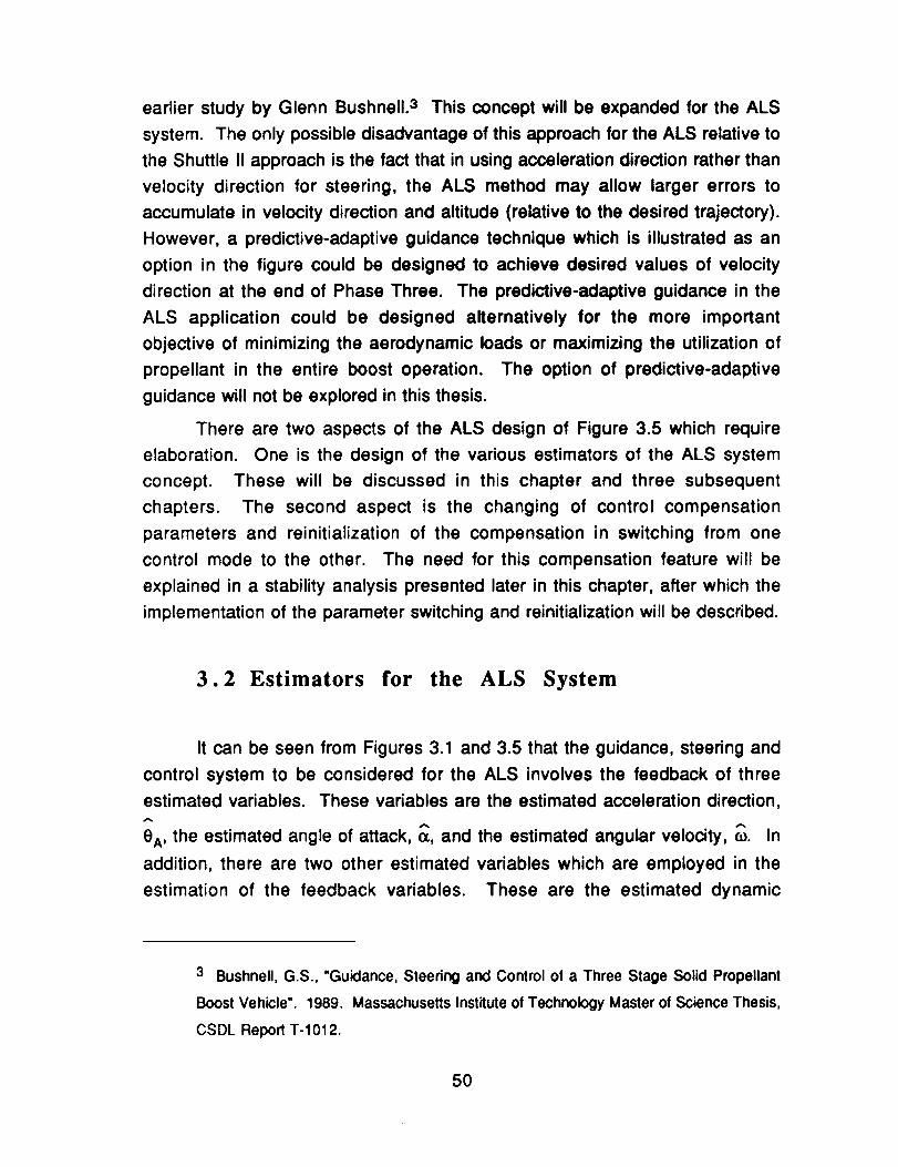
earlier study by Glenn Bushnell. 3 This concept will be expanded for the ALS

system. The only possible disadvantage of this approach for the ALS relative to

the Shuttle II approach is the fact that in using acceleration direction rather than

velocity direction for steering, the ALS method may allow larger errors to

accumulate in velocity direction and altitude (relative to the desired trajectory).

However, a predictive-adaptive guidance technique which is illustrated as an

option in the figure could be designed to achieve desired values of velocity

direction at the end of Phase Three. The predictive-adaptive guidance in the

ALS application could be designed alternatively for the more important

objective of minimizing the aerodynamic loads or maximizing the utilization of

propellant in the entire boost operation. The option of predictive-adaptive

guidance will not be explored in this thesis.

There are two aspects of the ALS design of Figure 3.5 which require

elaboration. One is the design of the various estimators of the ALS system

concept. These will be discussed in this chapter and three subsequent

chapters. The second aspect is the changing of control compensation

parameters and reinitialization of the compensation in switching from one

control mode to the other. The need for this compensation feature will be

explained in a stability analysis presented later in this chapter, after which the

implementation of the parameter switching and reinitialization will be described.

3.2 Estimators for the ALS System

It can be seen from Figures 3.1 and 3.5 that the guidance, steering and

control system to be considered for the ALS involves the feedback of three

estimated variables. These variables are the estimated acceleration direction,

0 A, the estimated angle of attack, _., and the estimated angular velocity, _. In

addition, there are two other estimated variables which are employed in the

estimation of the feedback variables. These are the estimated dynamic

3 Bushnell,G.S., "Guidance,Steering and Control of a Three Stage Solid Propellant

BoostVehicle". 1989. MassachusettsInstituteof TechnologyMasterof ScienceThesis,

CSDL ReportT-1012.

5O

pressure, (employed in estimating the angle of attack), and the estimated

angular acceleration (employed in estimating the angle of attack and the

angular velocity). The design of the estimators to generate these variables

involves consideration of (a) the reduction of adverse effects of signal errors

(e.g., quantization), (b) minimization of the effects of system modelling errors,

and (c) the effects of estimator design on speed of response and stability.

The designs of most of the estimators described in this thesis are highly

tentative, since the system and signal characteristics which influence the

configurations and parameters of these estimators have yet to be finalized for

the ALS. This is especially true for the angular velocity, angular acceleration,

and angle of attack estimators discussed in Chapters 4 and 5. The signal and

system characteristics have the least effect on the design of the dynamic

pressure estimator, which is described in Chapter 6.

3.3 Acceleration Direction Estimator

3.3.1 Introduction

The estimator which generates the estimated direction of the vehicle

acceleration (excluding gravity) is of primary importance in the design of the

acceleration direction guidance, steering, and control algorithm. The design

and implementation of this estimator involves the following steps:

(1) Computing the direction of the acceleration vector in body axes

from inertial measuring unit (IMU) accelerometer measurements.

(2) Expressing the direction of the measured thrust direction in terms

of pitch and yaw angles.

(3) Passing the pitch and yaw angles through first order low-pass

filters to generate filtered angles.

(4) Employing the filtered angles to generate a unit vector in body

axes representing the filtered acceleration direction.

51

(5) Comparing the unit filtered-direction vector with the commanded

acceleration direction (transformed to body axes) to compute the

pitch and yaw errors in acceleration direction.

An important feature of the acceleration direction estimator is step (3), the

filtering of the measured acceleration direction. This filtering is necessary to

reduce the control signal fluctuations caused by the effects of quantization in the

IMU accelerometer signals. In addition, filtering improves the control loop

stability by reducing the effects caused by the regenerative feedback of the

engine nozzle contribution to the estimated acceleration direction.

The acceleration direction is employed as a feedback variable in both the

pitch and yaw loops in the conventional version of acceleration direction

guidance, steering and control. However, in the ALS it will be assumed that this

direction is employed only in the pitch loop, and that the yaw angle of attack or

the sideslip angle is employed as the primary feedback variable for yaw control.

As pointed out previously, only the problems of pitch control will be considered

in this thesis. The possibility of using the acceleration direction estimator in

both pitch and yaw is not precluded by the design described below, which

includes both pitch and yaw angles of the acceleration direction vector.

3.3.2 Calculation Procedure

A

The commanded and estimated acceleration direction angles 9kc and eA

in Figure 3.5 are actually represented by unit vectors in the present simulation

of the ALS system. Initially the commanded acceleration vector, 0Ac, is

computed in the inertial frame and stored as a function of time (see Chapter 7).

Later, during actual in-flight simulations this stored acceleration vector is

retrieved and transformed into the body axis system. The estimated

acceleration direction angle, 0 A, is derived from IMU accelerometer

measurements employing relationships that will be described in this section.

The manner of computing pitch and yaw errors from these vectors will also be

described.

52

The estimated acceleration direction is based on inertial velocity

increments measured by the IMU. During each control cycle these inertial

measurements are transfered to the body-axis system. These three body-axis

increments are:

AV 1 = increment in velocity along the vehicle x (roll) axis

AV 2 = increment in velocity along the vehicle y (pitch) axis.

AV3 = increment in velocity along the vehicle z (yaw) axis.

These increments are employed as follows to compute the pitch and yaw

angles of the measured acceleration-direction vector, designated respectively

as j3p and _y.

_p = tan-1 (AV3/AVl)

_y = tan-1 (-AV2/AVl)

(3.1)

(3.2)

where the angles are defined positive according to the right handed rule.

These two acceleration-direction angles are then sent through a discrete low-

pass filter. In the continuous domain this filter has the form

J3(s) _ 1

(s) _l_S + 1(3.3)

where _p is the filter time constant. Using the Backward Rectangular rule the

complex frequency, s, can be approximated in the z-domain by the relationship:

s- 1 - z "1 (3.4)T

53

where T is the sampling time of the discrete filter. Substituting Equation (3.4)

into (3.3) results in the following two difference equations:

[3p = KI3 g "1 _p + (1 - Kp)pp (3.5)

_y -- K[3 z "I _y +(1 - KI3 ) _y (3.6)

where 13p,[_y are the filtered pitch and yaw angles, respectively, and where the

constant Kp is computed as

_p

KI_ - T + zp (3.7)

Finally, the unit vector, U A, representing the estimated filtered thrust

direction in body axes is computed from

A

U A = Unit value of

1

ta°( y)tan( p)

(3.8)

Designating the transformed unit vector representing the commanded

acceleration direction as UAc, the acceleration-direction errors EA, (pitch) and

EA_ (yaw) are computed as follows. First, the cross product between UAc andA

U A is obtained:

C m OA X MAc (3.9)

54

Then the angle, [3A, between the vectors is computed from

13A = sin "11C[ (3.10)

And finally, a vector representing the error angles is computed from

OF. = 13A [ unit (C)] (3.11)

The pitch and yaw error angles E,_ and EAy are then equal to

components of ME:

E_ = OF.: (3.12)

EAy = 0E3 (3.13)

The pitch error EA_ is represented by the symbol EA in Figure 3.5.

3.4 Approximate Vehicle Transfer FunctionsRelationships for Stability Analysis

Since the details of the vehicle bending and slosh modes and the

characteristics of the engine nozzle servos were unavailable at the initiation of

this thesis study, it was decided to represent the ALS by a rigid-body model,

assuming lagless engine nozzle servos. These assumptions make it an easy

matter to achieve large stability margins. This further justifies the use of

approximate dynamic models to adjust the compensation parameters.

The two control modes used in the ALS simulation are illustrated in

Figures 3.6 and 3.7. As shown in these figures the compensation design is

achieved by breaking the forward control path at the nozzle servo command. It

55

+

+

UJv

o (;

O

._O E

O,- E(1)

E""

_)

E_°--

X

oO.

(O

1,

56

W

• o

0.B

C

E0

0

e- t-o

-i D

°_-T"C c

"0

C 00 0

U

E_E--0 0

+

÷LIJ

\_C

uJ

f

_ __i _

W

°_

._E

x0O.O.

JI,,I.

57

was decided to design the compensation parameters to produce a 0 dB open-

loop crossover frequency of 3 rad/sec. This crossover frequency was chosen to

allow for adequate phase and gain compensation of the bending modes. For

the ALS it is assumed that the estimated first and second bending frequencies

are 13.8 rad/sec and 17.4 rad/sec, respectively. These bending modes are

based on data provide by the Boeing Aerospace Corporation for a vehicle

which is similar in design to the system being studied in this thesis. Also, the

chosen 0 dB crossover frequency is sufficiently high for rigid body stabilization,

being well above the maximum unstable pole frequency.

For the purpose of stability analysis, the following assumptions are made to

approximate the vehicle transfer functions:

(1) The transfer function between the attitude, 0, and the engine

nozzle deflection, 6, as derived in Appendix D and expressed in

Equation (D.13), is

(25 (3.14)

AS(S) {s 3 _(CI+C2) s2-C4s+C2C4}

where the incremental signs of Equation (D.31) have been

dropped for simplicity. In the vicinity of the chosen 0 dB crossover

frequency this transfer function can be approximated as

e(s)_ C5

2 2

where the two poles are based on the approximate relationship of

Equation D.37. Since the values of the quantity C1, as listed in

Table D.1 of Appendix D are very much smaller than those of C4,

this transfer function can be further approximated by the form

employed in Figures 3.5 and 3.6:

58

where

e (s)=.

(3.16)

}_ = C5 (3.17)

2 C4 (3.18)ir.ov =

The first-cut analytical computation of the compensation gains for

the two control modes will neglect (ov, whose maximum value is

roughly a factor of three below the chosen 0 dB crossover

frequency of 3 rad/sec. However, the computer generated

frequency response characteristics and the gain values based on

these characteristics will include the effects of _%.

(2) It can also be assumed that changes in vehicle attitude in the

vicinity of 3 rad/sec do not produce significant changes in the

earth-relative velocity direction, as represented by the flight path

angle 7. Since the pitch angle of attack in the absence of winds is

merely equal to the difference between 0 and 7, it can therefore be

assumed that

a(s) = 8(s) (3.19)

in this frequency range.

(3) The representation of the acceleration-direction feedback in

Figure 3.7 is simplified by assuming that this feedback is based on

the acceleration at the c.g. rather than the acceleration at the IMU

which is employed in the simulation studies.

59

3.5 Nozzle Command Conversion Relationship

As seen in Figures 3.6 and 3.7 the ALS flight controller generates a

single nozzle deflection command, 8c, based on the product of a gain, Ks/Kv,

and the attitude rate error. Ks is the constant inner loop gain and Kv is the

calculated vehicle gain. By dividing Ks by Kv the total inner loop forward gain is

held constant as the vehicle gain varies with time. The nozzle command, 8c,

illustrated in Figures 3.6 and 3.7 is based on the vehicle model illustrated in

Figure 3.8 where the nozzle hinge point is located along the roll axis of the

vehicle. According to Figure 3.8, the moment generated by a deflection of the

thrust vector is given by the expression

M = T sin 80 Xcg (3.20)

where T equals the total thrust of the core and booster stages.

For the ALS vehicle an equal pair of nozzle commands (8c and 8b) is

required from the flight controller such that the resulting moment due to the core

and booster thrusts is equal to the moment calculated from Equation (3.20).

From Figure 3.9 the moment generated by the ALS thrust vectors is given by the

relationship

M = (T b + To)sin(8)Xcg-T b cos(8)(D + zc, ) - T c cos(8)zc, (3.21)

The thrust of the core and booster can be represented as a fraction of the

total thrust by the expressions

T b = T n_) and T c = T n_nb+ nc nb+ nc (3.22)

where n b and nc are the number of operating booster and core engines

respectively. Substituting Equation (3.22) into Equation (3.21) results in

6O

M T sin (5) Xcg " T c°s (_) I'---E'L- (D + zc_l + -Zcg= _n b + nc nb+ n c(3.23)

Figure 3.8

M

Xcg

Single nozzle deflection configuration.

Define

.c 1A= -n--la-----(D + Zcg}+- --Zcg+ 13c lab + IIc

(3.24)

Then Equation (3.24) can be written as

M = T sin (5)x,,- T cos (5) A(3.25)

Setting Equation (3.20) equal to Equation (3.25) results in

- T cos (5) A = T sin (5 3 ×c,T si. (_)_cg(3.26)

61

As previously mentioned in Chapter 2 the nozzles of the core and

booster engines are installed at a fixed cant angle, C. The nozzle deflection as

t+x

Figure 3.9

Tb"

Xcg

T÷Z

Moment generated by ALS nozzle deflections.

defined in Figure 3.9 can therefore be redefined in terms of the installed cant

angle by the relationship

8 = (5c + C) (3.27)

Substituting Equation (3.27) into (3.26) and eliminating the total thrust, T,

results in

sin /5otan (5c+C)= Am+

xcg cos (5c+C) (3.28)

62

Assuming that cos(Sc+C) = 1, the relationship for the commanded nozzle

deflection is given by:

°18 c = tan (xc-_g+sin 8o)-C

(3.29)

Further, assuming that the nozzle deflection, 5 o, is small, then the

commanded nozzle deflection can be approximated by

where

_ic = 8o + _Bias (3.30)

_Bias = _ - CXcg

The commanded nozzle defections for both the core and booster is,

therefore, a function of the multiplicative gain, KdK v, as well as an additive bias

term, 6Bias. The block diagram for determining the commanded nozzle defection

for the ALS simulation is shown in Figure 3.10. In analyzing the stability issues

of both the acceleration-direction control mode as well as the Qo_ limiting control

mode, the effects of the additive bias term are neglected. Consequently, 5Bias is

not included in either Figure 3.6 or Figure 3.7.

_Bias

_c

Figure 3.10 ALS nozzle command block diagram.

63

3.6 Approximate Transfer Functions for the Qa-Limit Mode

Utilizing the above simplifying assumptions along with other

assumptions, the approximate transfer function model of the ALS shown in

Figure 3.6 can be employed to analyze the critical frequency response near the

0 dB crossover for Phase One, Phase Two and the Qo.-limit mode for Phase

Three. This transfer function model neglects the effects of sampling, assumes

perfect measurements and estimations of feedback variables, and employs the

same control compensation gains for the control modes of the three flight

phases. An integral-plus-proportional compensation operates on the attitude

errors Ee and E_, to obtain a signal which is combined with the estimated

angular rate. The resulting signal is then multiplied by a proportional gain

equal to K_Kv to generate the engine nozzle command.

The open-loop transfer function of Figure 3.6, determined by breaking the

inner loop in the forward path, is expressed as follows:

S S 2 _ 032(3.31)

This open-loop function will be employed, with and without the

superimposed effects of sampling, in computer studies of the frequency

response of this mode. As mentioned previously, first-cut analytical

comparisons of the two control modes will neglect the effects of 03v to simplify

the analysis.

3.7 Approximate Transfer Functions forAcceleration Direction Feedback Mode

Employing the same assumptions as in Figure 3.6, a second

approximate transfer function model shown in Figure 3.7 can be employed to

describe the critical frequency response characteristics for the acceleration-

64

direction feedback mode of Phase Three. This diagram differs from that of

Figure 3.6 in its addition of another feedback variable, the estimated (filtered)

deflection of the acceleration vector relative to the x-axis, Be&. When this

variable is added to the attitude e of the x-axis relative to the local geographic

A

coordinate frame the estimated acceleration angle 6% relative to the local

coordinate frame is obtained. This estimated acceleration angle is then

subtracted from the commanded acceleration angle 6Ao to generate the

acceleration-direction control error E A.

The derivation of the transfer function relationships for the additional

acceleration direction feedback signal Ae A is as follows. First, it is noted that the

acceleration normal to the x-axis in the pitch plane may be approximated by the

sum

-F_i + SQCncz(zaNormal = (3.32)

M

and that the net axial acceleration may be expressed as

F- SQCaaAxial = (3.33)

M

Second, assuming that aNormal << aAxia I, it is noted that the angle of the

acceleration vector relative to the vehicle x-axis in the pitch plane can be

approximated by

AOA = aN0rm_l (3.34)aAxial

Substituting Equation (3.33) and (3.32)into Equation (3.34) results in

65

F - SQC a(3.35)

Third, approximating the discrete low-pass filter of the acceleration

direction estimator by a continuous low-pass filter with a time constant Zp, the

Laplace transform of the additional filtered feedback signal ASA_(S) is related to

the unfiltered ASA(s) by

AOA,(s) ---[ZpSl+ 11 A_A(s) (3.36)

The open-loop transfer function of Figure 3.7, determined by breaking the

inner loop in the forward path, is expressed as follows

- (sG° (s) = __ v $2 2- co v

_s+l

Fso .t(.°'- s+l

(3.37)

This transfer function will be employed to study the effects of compensation

gains on the open-loop frequency response, with and without the effects of

sampling. However, in order to obtain an insight into the differences between

the acceleration-direction control mode and the Qo_-Iimit mode, some further

approximations will be introduced. These are described below.

In the vicinity of the 0 dB crossover frequency of 3 rad/sec CJo(s) may be

simplified as follows:

First, assuming _13= 5 seconds,

66

. 1 1 _=_ l ,/ _90 o + 3.8 o___- 113s+ l.ls=Jco 15103 jl5 (3.38)_--3

or

[;_ 1 t =_1_13s + 1 s- j3 1:1_s (3.39)

Employing the approximation of Equation (3.39) and neglecting _ in Equation

(3.37), the transfer function becomes

F s2tIFsQca](3.40)

Second, assuming the same value of x13= 5 seconds, it can be shown

that for close to maximum aerodynamic effects, based on Q = 790 psf, the term

enclosed by the first brackets in the third term of Equation (3.40) is

approximately unity when co= 3 rad/sec:

1 + l _,F - SQCa] s = j3, Q = 790 psf

= [l-j 0'10951=[1-j 0.0365]=1 (3.41)

Hence, Equation (3.41) can be approximated as

67

(3.42)

Factoring out Kv/S2 from Equation (3.42) and rearranging terms, the

open-loop transfer function near 3 racl/sec becomes

Ks F o,s, soc.l+ _ 1 KEI/KE{F FQCa) +lq, -

(3.43)

This open-loop function and the other open-loop function of Equation

(3.31) with o)v = 0 will provide the starting bases in the next section for a first-cut

analytical comparison of the problems of compensation gain selection in the

two control modes represented by these functions.

3.8 Approximate Analytical Stability AnalysisWithout Sampling Effects

The purposes of the following approximate analyses are (1) to provide an

insight into the aspects that influence the selection of compensation gains for

the two control modes of Phase Three and (2) to show how the compensation

gains of the two modes must differ because of the role of the engine nozzle

deflection in the acceleration direction feedback. The open-loop transfer

functions expressed in Equations (3.31) and (3.43) provide useful insights into

the effects of compensation gains on stability. These transfer functions will be

68

examined individually, first considering the case where there is no integral gain

and then considering the problem of adjusting the integral gain along with other

gains.

Proceeding first to the determination of gains for the Qo_-Iimit mode as

represented by Equation (3.31). Assuming that (0v is zero, and letting the

integral gain, KEI, also equal zero, the open-loop transfer function then

becomes.

Go(s)= +s]S2 (3.44)

It can be shown that the values of KE and Ks required for a phase margin

of L_(_m at a 0 dB crossover frequency are solutions of

tan AtOm "- (00

KE (3.45)

and

[K2E+ (002] ]/2 K___=1 (3.46)2

(0o

Solving these relationships for a chosen phase margin of 45 ° yields

(00

KF-"- tan (A_)m) = 3 sec "1 (3.47)

and

69

2

K s - coo = 2.121 (3.48)

The next step in this approximate design procedure is to select a value

for the integral gain KEt. Using Equation (3.31) and letting oh_= 0 results in the

new open-loop transfer function

Oo,s,;,,[s+KE+ (3.49)

K E is _, the effect of introducing KEI is to reduce the

phase margin to a value ASm, which is a solution of

KEI

i --' _9tan A_ m = (3.50)

Selecting a value of 35 ° for the new phase margin yields an integration gain of

KEI = coo coo - K E tan ASm = 2.698 sec "2 (3.51)

In order to maintain the 0 dB crossover at 3 rad/sec with the added effect of KEt it

is necessary to adjust K_ to satisfy

IK2CKE' 211'2 o/+ - K___s= 12E _o ,'-_---,.

_o

(3.52)

70

therefore

2

K 8 = °°o = 2.458 sec "2

(3.53)

The gain margins based on the above compensation gains for the open-

loop function of Equation (3.49) are adequate. The high frequency margin is

infinite and the low-frequency margin is 8.7 dB.

Although the above values of the compensation gains will be significantly

revised in the subsequent computer studies, these approximate values are

useful for comparison with similarly determined values for the acceleration

control mode. For the acceleration-direction mode it will be recalled that the

open-loop function may be approximated by

K_ s

(3.54)

Except for the terms in the brackets which multiply s and K E, this open loop

function has the same form as the Qa-limit mode, given by Equation (3.49):

Go (s) = K--_-[s + KE + K--_ ]S 2 S J

(3.55)

In fact, both open-loop functions can be expressed in the general form,

71

$2(3.56)

where for the Qoc-limit mode,

K1 = Ks (3.57)

K2 = Ks KE (3.58)

K3 = Ks KEI (3.59)

and for the acceleration-direction mode,

K2 sQc,K3 = Ks Km (3.62)

Equations (3.57) to (3.62) indicate that only two of the open-loop function

coefficients, K1 and K2, are affected by the choice of control mode. Furthermore,

analysis has shown that only one of these coefficients, K1, is affected

appreciably. Thus, assuming vehicle parameters for a trajectory point where Q

is close to a maximum, assuming '¢p -- 5, assuming KE = KE, KEI-KEI, and

Ks--Ks in Equations (3.60) to (3.62), and substituting the above determined

values of K E, KEI, and Ks into Equations (3.57) and (3.59), it is found that in

going from the Qc_-Iimit mode to the acceleration-direction mode

(I) The value of K1 is reduced by roughly 18% from 2.457 to 2.018

and

72

(2) The value of K2 is reduced by only about 5% from 7.371 to 6.976.

Using the above values of K1 and K2 for the acceleration-direction control

mode along with the original value of K3 it is found that the 0 dB crossover

frequency is reduced from 3 rad/sec to 2.68 rad/sec and that the phase margin

is reduced from 35 ° to 22.9 o. This reduction in phase margin is sufficient to

suggest that that it may be necessary to change the compensation gains when

switching modes.

The compensation gains that would be required in the acceleration-

direction control mode to produce the same K1, K2, and K3 values that result

from given K E, KEI, and K8 values in the Qa-limit mode can be computed by the

following approximate procedure. First, assume that the close-to-unity factor in

Equation (3.61) is equal to a constant Co, defined as

j - (3.63)

Then, employ C o in Equation (3.61) to solve for KE:

F_E= K2- / C° (3.64)

K8

Next, substitute this expression into Equation (3.60) and solve the resulting

relationship for Kg

-(3.65)

73

Finally, using the value of K s computed from Equation (3.65), compute K E from

Equation (3.64) and compute KEI from Equation (3.62).

Employing the above procedure for the chosen point on the trajectory

yields values of

K s = 2.921

= 2.666

=2.270

These compensation gains resultin KI, K2, and K3 values thatare within0.4%

ofthe originalvalues forthe Qo_-limitmode.

Itwillbe shown in Section 3.10 thatthe transientproduced by changing

the compensation gains as the controlmodes are switched can be minimized

by a procedure forreinitializingthe controlintegratorso thatthe engine nozzle

command does not change when the compensation gains are altered. Before

proceeding to thismethod of accommodating the gain changes, the values of

the gains required willbe determined by a more accurate analysis which

includeshigher order terms and the effectsofdigitalsampling.

(as compared to Ks = 2.458)

(as compared to KE = 3)

(as compared to KEI = 2.698)

3.9 Approximate Stability Analysis with SamplingEffects

To include the digital sampling effects in the preliminary analysis

presented above a control design software package, MATLAB, was utilized. A

single sampler was assumed to operate on the engine nozzle command. The

frequency response analysis was facilitated by the decision to employ a single

sampling period of T=0.1 seconds for the guidance, steering, control, and

estimation. The use of the single sampling period for all operations also

facilitated the implementation. Although the first cut computation of the

compensation gains for both modes neglected O_v, the following computer

74

generated analysis includes this effect. As discussed in Appendix D (Equation

D.37) the approximate locations of the maximum unstable poles is given by

s= cV-

This relationship can be further simplified by noting from Table D.1 that the

values for C1 throughout Phase Two and Three are in general much smaller

than C4. As a result, the first term on the right side of the above equation can be

eliminated so that the maximum unstable pole frequency is approximately equal

to the square root of C4. As shown in Table D.1, the value of the unstable pole

frequency is small during the beginning of Phase Two (t=8 sec) and Phase Four

(t=120 sec), but comparatively large during the midpoint of Phase Three.

The peak value of C4, which occurs at approximately 90 seconds after

ignition, represents the point in the trajectory when the vehicle is at its most

unstable state without control feedback. Typically this period occurs at or near

the maximum dynamic pressure when the combined effects of the air-relative

velocity of the vehicle and the air-density are most critical. Consequently, the

vehicle state at 90 seconds was chosen as the critical operating point at which

the control gains would be selected. In this manner, the resulting phase and

gain margins should theoretically be acceptable for the remaining points along

the trajectory

In applying the sampled data analysis to recompute the compensation

gains it was decided to choose these gains to produce an open-loop function

whose corresponding closed-loop function yields a peak magnitude close to 5

dB for both control modes at 90 seconds. This criterion necessitates increasing

the phase margin to about 40 °, increasing the low frequency gain margin to

above 12 dB and increasing the 0 dB crossover frequency ((%) up to a

maximum value of 4.3 rad/sec.

It was found that these frequency response requirements could be met

with a single set of three constant control gains for each control mode. These

gains are given in Tables 3.1 and 3.2. Employing these gains at various points

for both control modes produced the values of phase margin, low frequency

gain margin (GM1), high frequency gain margin (GM2), 0 dB crossover

75

frequency, and peak closed-loop magnitude presented in Tables 3.3 and 3.4.

Nichols plots of both the open-loop characteristics at 90 seconds are given for

the two control modes in Figures 3.11 and 3.12.

These frequency response characteristics were obtained with an

approximate vehicle system which assumed perfect nozzle actuators as well as

other simplifications. The inclusion of a nozzle actuator transfer function could

significantly reduce the 0 dB crossover frequency, the phase margin, and the

high frequency gain margin, and thereby require some adjustments in the

compensation gains. Moreover, the inclusion of bending and slosh modes may

require not only the adjustment of the three compensation gains but also the

addition of one or more compensation filters.

Time

(sec)Phase

Margin

Low Freq.

Gain Margin

(GM1)

High Freq.

Gain Margin

(GM2)

(oc Peak

Mag

8 42.530 18.359 15.720 3.845 4.544

66 41.863 14.570 15.725 3.723 4.805

90 41.344 12.651 15.728 3.635 5.019

42.156 15.723120

Table 3.1

3.77615.983 4.688

Stability statistics for Qo: limiting mode at different critical

times in the trajectory.

Name

KE

Value

2.700

KEj 0.917

K_

Table 3.2

3.276

Selected gains for Qo_ limiting mode.

76

Tlme

(sec)Phase

Margin

Low Freq.

Gain Margln

(GM1)

High Freq.

Galn Margin

(GM2)

o)C Peak Mag

8 43.378 19.384 14.673 4.279 4.330

66 42.750 13.707 14.515 4.158 4.735

90 42.610 11.405 14.351 4.092 5.014

44.887

Table 3.3

120 16.446 14.191 4.341 4.224

Stability statistics for acceleration-direction steering mode

at different critical times in the trajectory.

Name Value

KE 2.394

KEI 0.794

4.390

Selected gains for acceleration-direction steering mode.

K_

Table 3.4

77

3O

2O

rn"o 10

"O

"- 0

-10

-20-260

" i i i

-240 -220 -200 -180 -160 -140 -120

Phase (deg)

Figure 3.11 Nichols plot for Q_t-limiting mode at t--90 see.

40

rot"1o

"1o

3O

2O

10t-"

tO_ 0

-10

GM1

-2O i i

-280 -260 -240 -220 -120

GM2 PM_

i I I

-200 -180 -160 -140

Phase (deg)

Figure 3.12 Nichols plot for acceleration-direction mode at t-90 sec.

78

3.10 Control Gain Reset Procedure for Mode

Switching

Section 3.8 and 3.9 have shown that the dynamics for the acceleration-

direction control mode and the angle of attack (or Qcz-limit) control mode are

different. Because of this difference, different control gains had to be selected

for each mode to achieve the same relative stability margins in both modes.

A problem with having different control gains for each mode is that during

switch-over a transient is produced in the commanded nozzle deflection. This

transient can be minimized by reinitializing the integrator every time the mode is

switched so that the new commanded deflection after switching equals the

commanded deflection just before switching. Thus, the integrator must be

reinitialized so that

5c = 5c (3.66)

where 5c is the commanded nozzle deflection during Q(z limiting mode, and 5c

is the commanded nozzle deflection in the acceleration-direction steering

mode. Each nozzle deflection command can then be expanded and expressed

in terms of its respective gains. For 5c this results in

_c =_(3.67)

For 5c the relationship is

where

5c K_= + + (3.68)

79

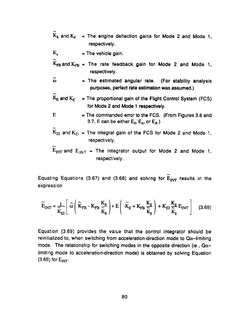
Ks and K_ = The engine deflection gains for Mode 2 and Mode 1,

respectively.

= The vehicle gain.

l(,_andK+--a = The rate feedback gain

respectively.

=

]_ and

E

for Mode 2 and Mode 1,

The estimated angular rate. (For stability analysis

purposes, perfect rate estimation was assumed.)

= The proportional gain of the Flight Control System (FCS)

for Mode 2 and Mode 1 respectively.

= The commanded error to the FCS. (From Figures 3.6 and

3.7, E can be either Ee, Ea, or EA. )

K_ and KEI -- The integral gain of the FCS for Mode 2 and Mode 1,

respectively.

F-,u_n-and EIN T -- The integrator output for Mode 2 and Mode 1,

respectively.

Equating Equations

expression

(3.67) and (3.68) and solving for F_,_ results in the

_.zl<r = 1___[ _( KFs-KFB K,)(=- +E -I_E+KFB_

Ks K6K,j+ KE[ =- EIN T

Ks(3.69)

Equation (3.69) provides the value that the control integrator should be

reinitialized to, when switching from acceleration-direction mode to Q(x-limiting

mode. The relationship for switching modes in the opposite direction (ie., Qa-

limiting mode to acceleration-direction mode) is obtained by solving Equation

(3.69) for EINT.

8O

(3.70)

The effect of resetting the control gain during control mode switching is

clearly illustrated in Figures 3.13 and 3.14. As shown in Figure 3.13 the control

integrator is reset at two points. The first point occurs approximately 34 seconds

after ignition and corresponds to a control mode switch from acceleration-

direction steering to Qa limiting. Following this control mode reset the vehicle

continues to fly under Qo¢ limiting control until approximately 95 seconds after

ignition, whereupon the vehicle returns to acceleration-direction steering and

the control integrator is again reset. Although the resetting of the control

integrator is very small at the first switching point, the second switch point (t = 95

sec) clearly shows a transient in the value of the integrator output. This

transient is necessary to maintain a smooth command to the nozzles during

control mode switching. The effect of resetting the integrator upon the

commanded nozzle deflection is shown in Figure 3.14. Although the shape of

the nozzle command is different once the vehicle has transferred back to

acceleration-direction steering, there is no step or discontinuity present at

switch over.

81

2

-IO

__-2

_3 ! I I I

20 40 60 80 100

Time (sec)

,__ I=0,Acceleration-directionMode._=1, Q(x Umiting Mode.

.... "_ .......... EI_i'E_ ..... .-CO"r:' .":ratoi .re.se.t........

120

Figure 3.13 Control integratorreset for control mode switching.

0

-0.5 ......................................................................"Ov

E° -IOO)

_-1.5

Control inteiator reset

-280 85 90

Time (sec)

I00

Figure 3.14 Nozzle command during control integrator reset.

82

Chapter Four

ANGULAR RATE ESTIMATION

4.1 Description

The manner in which the angular rate and other feedback variables are

to be generated is dependent on the design of the avionics system which has

yet to be fixed for the ALS. For the purposes of this thesis investigation it was

decided to assume that the only measurements available for generating

feedback variables are (1) the vehicle attitude relative to an inertial reference

frame measured by an inertial measurement unit (IMU), (2) the inertial velocity

of the vehicle measured by the IMU, and (3) the measured deflections of the

engine nozzles. It was further assumed that either a strapdown or a stabilized-

platform IMU could be employed, with either high or low performance

accelerometers and gyros.

In order to accommodate the wide range of possible IMU characteristics

this thesis develops feedback signal estimators that can deal with worst-case

levels of noise and/or quantization in the IMU signals. This means in the case

of the angular rate feedback signal that it is not sufficient to employ a rate signal

that is merely derived from the quotient of attitude change and the control

sampling period. This derived rate signal can have unacceptably large

fluctuations if the IMU measurements have large quantization or noise levels

and/or if there is a short sampling period.

One method for reducing these fluctuations is to employ a

complementary filter estimator which utilizes the derived rate signal in

combination with an estimated angular acceleration signal. This estimator

reduces the effects of quantization and noise in the attitude measurements by

employing the low-pass filtering of the derived rate signal to generate an

estimator rate signal that is accurate only at low frequencies. This low-

frequency signal is augmented by a high-frequency estimated rate signal

generated by the low-pass filtering of an angular acceleration estimate. The

83

effect of the low-pass filtering of the angular acceleration estimate is equivalent

to the high-pass filtering of a rate signal based on the integral of angular

acceleration. The angular acceleration estimate is based on the IMU-measured

velocity increments and the measured engine deflections, with an additional

correction for small errors in the modeling of the effects of thrust and

aerodynamic forces on angular acceleration. If the quantization and noise

levels in the IMU velocity measurements are sufficiently low, this rate estimator

can produce lower signal fluctuations than are contained in a derived rate

signal.

4.2 The Complementary Filter

A simplified continuous representation of a complementary filter is

illustrated in Figure 4.1. With this approach, the high frequency state estimate,

Xhigh, is passed through a high-pass filter while the low frequency state, £k,w, is

passed through a low-pass filter. The outputs of the two filters are then

combined to produce a single state estimate. Each filter attenuates unwanted

frequency components. Thus, the low pass filter attenuates high frequency

components and the high pass filter attenuates low frequency components. The

transfer function for the complementary filter has unity gain with no phase shift.

Consequently, in the ideal case where both the low and high frequency

estimates are exact, the complementary filter acts as a unity transfer function.

4.3 ALS Rate Estimation

Figure 4.2 shows a simplified continuous signal representation of the

ALS angular rate estimator. The low frequency estimate is passed through a

low pass filter. The high frequency component is obtained by first estimating the

angular acceleration of the vehicle. In effect, this signal is then integrated to

produce a high frequency estimate of angular rate and then filtered through a

high pass filter. In the actual implementation, the high frequency estimator path

combines the integrator and high pass filter to produce the simplified

continuous form of the rate estimator shown in Figure 4.3.

84

]K

Or equivalently,

X

low pass filter

;l '_s+ 1

high pass filter

+

+

Or equivalently,

low pass filter

Xlow frequency ¢S + 1

h,gh,,.qu.no,Ihigh pass filter

+

X

Figure 4.1 Block diagram development of complementary filter.

85

OLow Freq 1: S + 1

'ts+l

0High Freq

,°

OHigh Freq

A

Figure 4.2 Continuous ALS rate estimator

I

eLowF,_q =! 1I 'ts+l

°,

eHigh Freq

Figure 4.3 Simplified continuous ALS rate estimator.

The accuracies of both the low and high frequency estimates are affected

by measurement noise. In addition, the accuracy of the high frequency estimate

is affected by errors in the modeling of the vehicle. One category of

mismodeling errors that is of particular concern in the case of the ALS is the one

that results in constant or slowly varying bias errors in the estimated angular

86

acceleration. Such a bias can be produced, for example, by an unmodeled

offset of a thrust vector as illustrated in the bottom diagram of Figure 4.4. If this

offset is ignored, as shown in the top diagram of Figure 4.4, the estimated

contribution to angular acceleration of the thrust will be in error by the product of

the thrust times the offset divided by the moment of inertia perpendicular to the

plane of the offset. This error amounts to a constant bias in the estimated

angular acceleration that produces a corresponding bias in the estimated

angular rate. As can be seen from Figure 4.3, an acceleration estimate bias,

eSms, would result in a steady state bias in estimated rate of _:eSias. TO remove

the modelling error, an additional feedback loop for acceleration bias correction

is added to Figure 4.3. This correction loop which is illustrated in Figure 4.5, is

based on a concept developed by James Herner of Autonetics.

As shown in Figure 4.5, the correction for the estimated-acceleration bias

is derived from the difference of two acceleration estimates. The first estimate,A "7.

_1, is the derivative of the estimated angular rate. The second estimate, o_2, is

the corrected estimate of angular acceleration.

(_Measured - 0

acg

_Measured = 0

Thrust

_eThrust > 0

I

r acg j

_'Thrust vector misalignment

Figure 4.4 Thrust vector misalignment contribution to estimated rate.

87

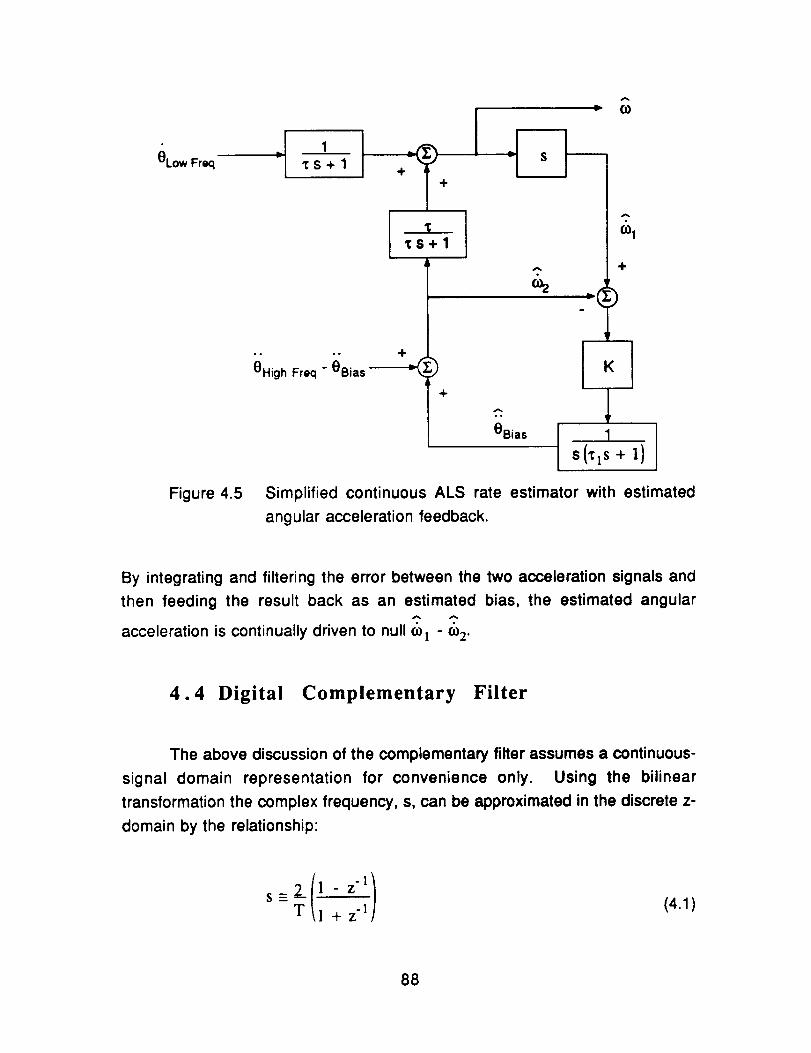
Figure 4.5

¢s+l I + +

oo °° "1"

OHigh Freq " eBias <

_s+l

A

+

A

(01

÷

r

A°o

OBiasI

[ s ('_1s + 1)

Simplified continuous ALS rate estimator with estimated

angular acceleration feedback.

By integrating and filtering the error between the two acceleration signals and

then feeding the result back as an estimated bias, the estimated angular

acceleration is continually driven to null (0] - (02.

4.4 Digital Complementary Filter

The above discussion of the complementary filter assumes a continuous-

signal domain representation for convenience only. Using the bilinear

transformation the complex frequency, s, can be approximated in the discrete z-

domain by the relationship:

T +z-](4.1)

88

where T is the sampling time of the discrete filter. Substituting Equation 4.1 for

s into Figure 4.1 results in the digital filter illustrated in Figure 4.6

For the ALS the measured quantities used to estimate angular rate are

the following:

1)

a)

The incremental change in attitude over the sampling instant of 0.1

sec. : The change in attitude about the pitch axis, ASy, is computed

in the following manner assuming a single-rotation-axis

maneuver.

The transformation from initial to commanded body axes is

computed by:

Body Last = r (4.2)

where

clnertialBody = the direction cosine matrix relating the current

transformation from inertial to body coordinates.

(C_-(_'d_ast)T = the transpose of the direction cosine matrix relating

the transformation from inertial to body coordinates computed at

the last sampling period.

b) It can be shown that for a single-rotation-axis maneuver where the

angle of rotation between the present and past commanded

orientations is small, the incremental roll, yaw, and pitch

components of rotation are given by:

z&Ox = (023- 032)2 (4.3)

89

low pass filter

A

Xlow frequency

Xhlgh frequency

T 1 ÷Z "1

2_+T 1 .(2_ + T) Z-1

_._23._ 1 - z1

2_+ T 1 "(2t+T)Z-1

high pass filter

÷

(_)_X

+

or equivalently

Xlow frequency

Xhlgh frequency

1

1-(2¢ +T)Z 1_X

Figure 4.6 Digital Rate Estimator.

90

Aex -- (c31 - c13)2 (4.4)

Aex -- (C12- C21)2 (4.5)

Body Lastwhere C(m,n) is an element of the transformation C Bodt ,

relating past to present body axes. The subscripts m and n

represent the row and column locations of each element. 1

2) The incremental change in velocity over the sampling instant of

0.1 sec.: The incremental change in velocity produced by external

forces (not including the effects of gravity) is determined first in

inertial axes, based on IMU accelerometer measurements, and

then is transformed into body axes using the current inertial to

body axes transformation. The resulting incremental velocity

vector, AV, has components AV x, AVy, and AV z along the roll,

pitch, and yaw axes, respectively.

3) The sensed angular deflection of the core and booster nozzles:

(The flight computer generates the same nozzle deflection

command to both the core and booster, so that 5y is the pitch axis

component of both equivalent nozzles.)

4.5 Low Frequency Angular Rate Estimate

The low frequency estimate of angular rate is computed by dividing the

incremental change in attitude over the control cycle by the sampling time, T:

1 Stubbs, G. S.," Final Report, Fiscal Year 1974 Advanced Targeting and Software

Design Studies." August 1974. C.S.D.L. Report R-838.

91

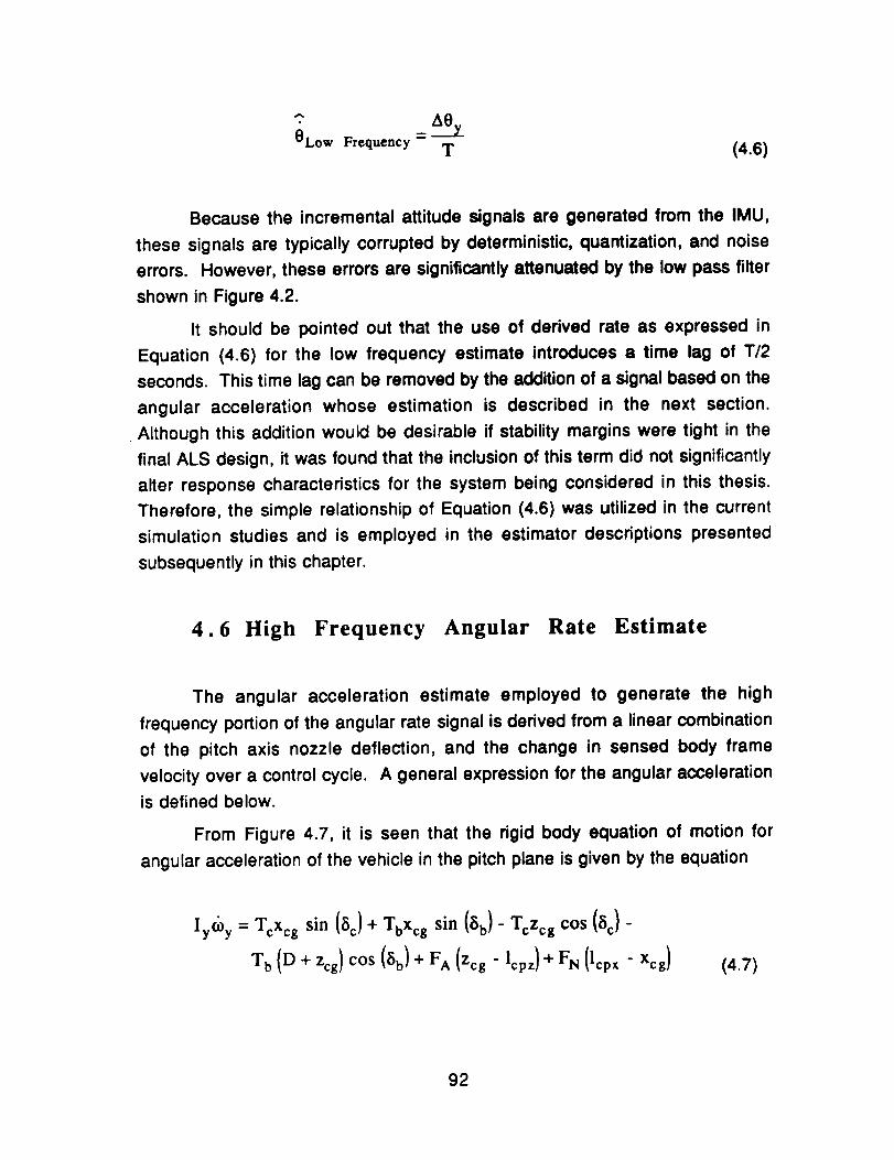
,3.

OLow Frequency -- AOyT (4.6)

Because the incremental attitude signals are generated from the IMU,

these signals are typically corrupted by deterministic, quantization, and noise

errors. However, these errors are significantly attenuated by the low pass filter

shown in Figure 4.2.

It should be pointed out that the use of derived rate as expressed in

Equation (4.6) for the low frequency estimate introduces a time lag of T/2

seconds. This time lag can be removed by the addition of a signal based on the

angular acceleration whose estimation is described in the next section.

• Although this addition would be desirable if stability margins were tight in the

final ALS design, it was found that the inclusion of this term did not significantly

alter response characteristics for the system being considered in this thesis.

Therefore, the simple relationship of Equation (4.6) was utilized in the current

simulation studies and is employed in the estimator descriptions presented

subsequently in this chapter.

4.6 High Frequency Angular Rate Estimate

The angular acceleration estimate employed to generate the high

frequency portion of the angular rate signal is derived from a linear combination

of the pitch axis nozzle deflection, and the change in sensed body frame

velocity over a control cycle. A general expression for the angular acceleration

is defined below.

From Figure 4.7, it is seen that the rigid body equation of motion for

angular acceleration of the vehicle in the pitch plane is given by the equation

IyCOy = Tcxcg sin (_c) + Tbxcg sin (fib)- Tczcg cos (8c)-

T b (D + zcg)cos (fib) + FA (zcg- lcpz)+ F N (lcp x - xcg) (4.7)

92

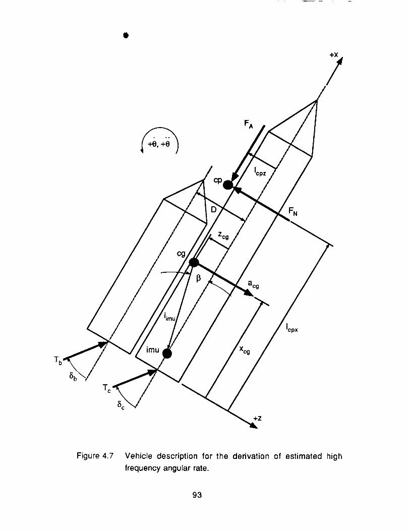
i

mb

cg

Xcg

+Z

F N

Icpx

Figure 4.7 Vehicle description for the derivation of estimated high

frequency angular rate.

93

where

ly =

Tc =

Th =

Sb =

Xcg =

Zcg =

D =

Icpx =

Icpz _--

V A .-

FN =

Pitch axis moment of inertia.

Core thrust.

Booster thrust.

Core pitch axis nozzle deflection.

Booster pitch axis nozzle deflection.

Body x axis center of gravity position.

Body z axis center of gravity position.

Distance between centerline of core and booster.

Body x axis distance from the centerline of the core to the

center of pressure.

Body z axis distance from the base of the core to the center

of pressure.

Axial aerodynamic force.

Normal aerodynamic force.

A second equation can be written which relates the linear acceleration at

the center of gravity along the body z axis to the normal aerodynamic force and

the body z axis component of the engine thrusts. That is,

macg =-F N + T c sin (8c)+ T b sin (Sb) (4.8)

The acceleration at the center of gravity can be related to the

acceleration as seen at the IMU by the following expression.

acg = aim u + limu(0 2 sin (13)-limud) cos (J3) (4.9)

94

Substituting the expression for a_ given by Equation (4.9) into Equation (4.8)

and solving for F n and then substituting this expression for F n into Equation (4.7)

and solving for (b yields:

(by = 1 (Tclcp x sin (8c)+ Tblcp x

Iy - m (lcp x - Xcg ) lim u

TcZcg cos (8c)- T b (D + Zcg) cos (_b)- maimu (lcpx

-m (lop x xcg ) lira u sin (13)my (4.1o)

Let

TclcpxK1c =

ly - m (lcp x - Xcg ) lira u (4.11)

Tblcpx

Klb = Iy - m (lcp x - Xcg ) lim u (4.12)

m0cp,,-x,,)K 2 =

Iy - m (lcpx - Xcg ) lira u (4.13)

K 3 =m (lcp x - xe$ ) lira u sin (13)

Iy - m (lcp x - Xcg ) lim u (4.14)

K4c = TcZc$

Iy - rn {lcp x - Xcg ) lira u (4.15)

T (D+,,,)K4b = Iy m (lcp x - Xcg ) lira u (4.16)

95

Then Equation (4.10) can be expressed as

_y2

= Klc sin (8c)+ Klb sin (Sb)- K2 aimu- K30y

K4c cos (Bc)- K4b cos (Sb)+ FA (Zcg-lcpz) (4.17)

By integrating _y over a sampling interval and then dividing by the

sampling period, the average angular acceleration is obtained:

t n1 f_y dt= 0avgn-1 (4.18)

where t, is the present sampling instant and tn-1 is the preceding calculation

time. Substituting Equation (4.17) into Equation (4.18),

It B I t R0avg=_ Klc sin(Sc) dt + I_T Klbsin(Sb) dt -t n-I n-I

l K 2aim udt 1 K3 2 dt - l K4cCOS(Sc) dtT T COy T

t n-I a-1 a-I

t n I t n

1 d, + IK4b COS -- F A (Zcg-Icpz) dt

n-I T n-I (4.19)

The integrals on the right side of Equation (4.19) can be approximated by

the expressions

t n

1 Klc sin (8c)dt = Klc sin (8c)¥a-I

n-I

(4.20)

96

it n

1 Klb sin {Sb)dt _=_ K,b sin (_b) n-,T n-I

If'"¥n-I

1 S 'n¥t u-1

K4c cos {8c) dt =

K4b cos (Sb)dt =

I% cos o-1

K4b COS (_b) n-I

(4.21)

(4.22)

(4.23)

The above relationships are based on the assumption that the nozzle deflection

over a sampling period is constant with time. The remaining integrals can be

approximated by,

¥n-l

"LI'°Tt n-1

K 2 aim u dt -= K 2 AVzT

(^2}2 dt -= K 3 COy n-1K 3 COy

(4.24)

(4.25)

.-.2

where COyis the previous estimate of angular rate as computed by the rate

estimator. The last term on the right side of Equation (4.19) is the component of

axial acceleration due to the axial aerodynamic force and the offset between the

center of gravity and the center of pressure. As an open loop calculation this

quantity may be difficult to estimate, primarily because the location of the center

of pressure (lcp z ) may not be accurately known. From a transient point of view,

however, it is possible to assume that the axial aerodynamic force will generate

an angular acceleration which is slowly varying. This is a good approximation

since both the center of gravity and Fa are slowly changing with time. Therefore,

the angular acceleration term generated by the axial aerodynamic force is

modelled for the moment as an unknown acceleration bias on the system.

Substituting Equations (4.20) through (4.25) into (4.19), and renaming the last

term on the right side of Equation (4.19) by the term a¢¢elblas, results in:

9 7 . ,.

0avg =Klc sin (_c)n-1 ÷ Klb sin (_b)n-l- K2 AVz -T

(^.)(4.26)

In the actual implementation of the rate estimator the term accelbi,, = of

Equation (4.26) represents not only the effects of the axial aerodynamic force,

F a, acting on a moment arm Xcg -Icp z, but also the effects of any errors in

modelling that combine to produce a slowly varying bias in the estimated value

of (]avg" This bias term is estimated and approximately corrected by the addition

of an angular acceleration bias estimation (AABE) loop to the estimator. The

implementation of this loop will be described in Section 4.7.

To obtain the change in attitude rate over time, Equation (4.26) is

multiplied by the digital sampling rate. Thus,

AOHigh Frequency = Oavg T (4.27)

The digital lagless filter illustrated in Figure 4.6 can be implemented by

substituting Equation (4.6) for the low frequency estimate and Equation (4.27)

as the high frequency estimate. The resulting block diagram is illustrated in

Figure 4.8.

4.7 Acceleration Bias Estimate

As discussed in Section 4.3, mismodeling errors in the high frequency

estimate of angular acceleration also result in errors in the estimation of angular

rate. To eliminate these errors an additional feedback loop was added to the

the continuous signal representation of the rate estimator shown in Figure 4.3

which resulted in the new rate estimator illustrated in Figure 4.5. As seen from

98

__,I I (++z-")IAe 2'_ + T l

T

2'c +T

1

1 - 2+"I" z'l2'¢ +T

IAOHigh Frequency

1

°.

(}avg

* acce Ibias

OO

Figure 4.8 Rate estimator without acceleration bias estimation

99

Figure 4.5 the estimation of unmodeled angular acceleration was computed

from the filtered difference of the estimated angular acceleration and the

derivative of the estimated angular rate. To emulate this procedure of

estimating unmodeled angular acceleration in the discrete signal

implementation a similar feedback loop is added to Figure 4.8 as shown in

Figure 4.9. As shown in Figure 4.9 the continuous integrator and low pass filter

of the angular acceleration loop have been replaced by their equivalent digital

implementations. In addition, o)1, which was computed in Figure 4.5 as the

derivative of the estimated angular rate is now computed as the back difference

of the estimated angular rate.

4.8 Frequency Response and TransientResponse

4.8.1 General

As seen in Figure 4.8, the rate estimator is a multi-input system.

Measured attitude, nozzle deflection, and AV signals are combined through a

lagless complementary filter to form low and high frequency estimates of the

angular rate. Both the low and high frequency estimates are modified by the

complementary filter whose time constant, _, determines its dynamic

performance. This time constant represents a relative weighting of the low and

high frequency paths. The larger the time constant the lower is the break

frequency of the low and high pass filters. For both low and high frequency

paths the choice of '¢ is driven by the considerations of measurement noise,

system stability, and steady state error of the estimate.

In addition to the effects caused by the complementary filter the effects of

the estimation of angular acceleration bias must also be considered. As shown

in Figure 4.9 the estimation of unmodeled angular acceleration is coupled to the

estimate of angular rate and vice versa. This occurs as a result of feeding back

the estimated unmodeled angular acceleration into the high frequency estimate

100

1_z-i2'_ +T

A_High Frequency

(0

T

°.

0avg

1 - Z"1

(1 + zl) cb31 - cb2 z1

Figure 4.9Rate estimator with acceleration bias estimation.

101

of angular rate. The effect of the estimated unmodeled angular acceleration

upon the high frequency estimate of angular rate is a function of the filtering

dynamics present in the AABE loop. The integral gain of the loop is determined

by the two constants cbl, and cb3. The low pass filter time constant is equal to

cb2. The choice of the integral gains and filter time constants for the angular

acceleration loop is driven by noise, tracking, and stability considerations.

4.8.2 Estimator Transfer Functions

To analyze the frequency response characteristics of the rate estimator

an approximate continuous model of the estimator is employed. As shown in

Figure 4.10 this is achieved by modifying the inputs to both the low and high

frequency paths of the rate estimator. In the high frequency path the

components of angular acceleration due to nozzle deflection, and AV are

replaced by the derivative of the true angular rate. In the low frequency path the

true angular rate is employed instead of AO/T. As a result, the effects of

measurement noise and parameter uncertainty are neglected in this estimator

model. Lastly, an angular acceleration input disturbance, d_, is added to the

loop to replace the bias in the estimated angular acceleration resulting from

errors and omissions in the modelling of the moments produced by engine and

aerodynamic forces.

Compared to the system illustrated in Figure 4.9 the simplified

continuous block diagram now has only two inputs, co and d_o. The frequency

response of the estimator can be analyzed by treating each input ,(0 and d_o

separately and deriving a set of continuous transfer functions in terms of the

output quantities _, _1, and d_b. Although it is possible to derive a total of six

transfer functions, only four are necessary to study the control issues. They are:

1+ K

s + 1)( s+ 1)= 1(0

1+ K

s + + 1) (4.28)

102

True anglar rate Estimated angular rate

.__.T,__'_S+I

(°2

031"_. +

=- 03

% K+ S ('_ls + 1)

Figure 4.10

03b = Unmodeled angular acceleration term(assumed to be slowly varying).

Simplified continuous rate estimator design loop.

A

_%_6_h

KS ('CIS + l)(_s + 1)+K (4.29)

A

03:2=

_b

-s (x]s + 1)('rs + 1)

s (x]s + 1)(xs + 1)+K (4.30)

A

0)-

6_b

( ls+ 1)s (x,s + l)('rs + I)+K (4.31)

103

The derivation of these transfer functions is described in Appendix E.

The continuous signal transfer functions presented in Equations (4.28) through

(4.31) are functions of the parameters K, tl, and _. In the actual implementation

of the estimator a discrete set of time constants and gains was employed as

illustrated in Figure 4.9. The relationships necessary to convert the continuous

signal parameters K, and 1;1 to the equivalent discrete signal values of cbl, cb2,

and cb3 are presented in Appendix F. The time constant _ is the same in both

the discrete and continuous representations. The next two sections will employ

the approximate continuous-signal transfer functions to explain the rationale for

choosing the values of _, K and 'c1 and then will examine the frequency

response characteristics produced by the values of these parameters chosen

for this thesis.

4.8.3 Rate Estimator Coefficients

The choice of 1; is influenced by two factors. First, there is the need to

filter out the effects of noise and/or quantization in the derived rate A6/'I" which is

used for the low frequency estimate of angular rate. This need places a lower

limit on the acceptable value of '_ and correspondingly places an upper limit on

the crossover frequency of the first order complementary filter. Second, there is

the need to minimize the effects of uncertainties in the parameters used to

generate °°2- This need suggests that the time constant _ be no higher than

dictated by the first requirement.

The choice of K and _2 in the angular acceleration bias estimation

(AABE) loop depends upon:

(1) The need to minimize the errors associated with tracking the bias

_o resulting from mismodeling of the angular acceleration. (A

higher value of integral gain, K, will generally improve the tracking

capability, however this is also at the expense of the stability of the

acceleration feedback loop.)

104

(2)

(3)

The need to filter the effects of noise and/or quantization on (o1.

(As shown in Figure 4.5, 0)1 is derived from the back difference of

the estimated angular rate divided by the sampling time of the rate

estimator. This form of differentiation is inherently "noisy" and can

adversely affect the estimated unmodeled angular acceleration.)

The need to maintain the stability of the unmodeled angular

acceleration feedback loop based upon the open loop transfer

function:

K

(4) The need to limit the errors in the estimation of the average

angular acceleration, 0)2. (An accurate measure of the angular

acceleration is needed for the estimation of the angle of attack.

See Chapter 5.)

4.8.4 Frequency Response Characteristics

The continuous signal gain and filter time constants chosen for the rate

estimator and their corresponding discrete signal values are shown in Table

4.1. The resulting frequency response characteristics for the approximate

continuous signal transfer function relationships will be examined below in

terms of the frequency response characteristics of the transfer functions

represented by Equations (4.28) to (4.31).

The significance of the identity relationship of Equation (4.28) is that for

the approximate continuous signal model of the estimator, the transfer function

between estimated and actual angular rate is unity, independent of the effects of

the angular acceleration bias estimator (AABE) loop. Of course, in the actual

estimator, where mismodeling produces gain as well as bias errors, the transfer

function between estimated and true angular rate will not be unity. However,

this function and its effects on ALS stability can be expected to be nearly

independent of the dynamics of the AABE loop.

105

Equations (4.29) to (4.31) define three other transfer functions that relate-?. -?.

the estimator variables cob, _, and ml to the angular acceleration bias term, _o.

The cancellation of this bias term and its effects on the estimated angular

Table 4.1

CONTINUOUS

K 0.50

'_1 1.2487

•¢ 0.245

DISCRETE

cbl

cb2

cb3

0.245

0.05

0.923

0.0385

Continuous and discrete rate filter constants.

,3.acceleration ¢o1 and estimated angular rate _ is the purpose of the AABE loop•

The ability of the AABE loop to achieve this purpose with the selected estimator

parameters is indicated by the frequency-response plots of Figures 4.11

through 4.13, representing the functions of Equations (4.29) through (4.31),

respectively.

The frequency response of (%/(_b shown in Figure 4.11 indicates the ability of

the estimated angular acceleration bias estimate, 0%, to track variations in the

bias ¢_b. This figure shows that sinusoidal variations in _ are well tracked by

the bias estimator for frequencies equal to or less than 0.1 rad/sec and that the

magnitude of o)o is essentially equal to that of _b up to 0.7 rad/sec. However,

the phase lag which starts out at roughly 10 ° at 0.1 rad/sec reaches an

unacceptable value of about 120 ° at 0.7 rad/sec. It may be concluded from

these results that the estimator provides acceptable performance out to a

106

frequency range of about 0.2 rad/sec. Fortunately, the bias to be estimated is

expected to vary at a slow rate that the estimator should be capable of tracking.

The effects of the ability of the AABE loop to cancel out low frequency

variations in ¢_o are shown in Figures 4.12 and 4.13. First, examining Figure

4.12 it is seen that the transfer function relating the estimated angular

acceleration co1 to ¢_b is well attenuated at low frequencies, having a magnitude

of approximately -30 dB at 0.1 rad/sec. Similarly, the transfer function relating

the estimated angular rate _ to ci}b is also attenuated at low frequencies, having

a magnitude of approximately -25 dB at 0.1 rad/sec.

4.8.5 Quantization Effects

As shown in Figure 4.9, the low and high frequency estimates of angular

rate are derived from measured Ae, AV, and _ signals.It is presently anticipated

that the Ae and AV signals will be provided by a strapdown IMU whose ring

laser gyros provide medium to high quality Ae signals. However, the estimators

100

--- 0¢-

-10010-1

v r v v v _ v _ v _ v v v _ v u v v | v v u v v

10o 101 102

Frequency (rad)

0

-100

-200r-

Q.-300

10-1 10o 101 102

Frequency (rad)

A

Figure 4.11 Frequency response of o_o/6_b.

107

50

"0

•-- 01-

-5010-2 10-1 10o

Frequency (rad)

I 1 ! ! l I ! i

, ; ; ; ; ; ;;

10_

10-2 10-1 10o 101

Frequency (rad)

A

Figure 4.12 Frequency response of o2/d_b.

50

"0

e- 0

50 .........lOq 10o 101 102

Frequency (rad)

0A

-100

-20Oi-

n

-30010-1

, , , , , , i . . , . , . . .

10o 101 102

Frequency (rad)

Figure 4.13 Frequency response of _/d,_b.

108

employed in this thesis study are designed to accommodate also the lowerquality A0 signals that would be generated by the electrical resolvers of a

stabilized-platform IMU.

It is assumed that the requirements of ALS guidance and control would

be adequately sewed by ring laser gyros whose primary error source affecting

estimator performance is an attitude signal quantization that ranges from 3

arcsec to 11 arcsec. In the case of the stabilized-platfrom IMU it is assumed that

the use of resolvers to measure attitude would increase the signal quantization

to 110 arcsec. Also, the effects of signal noise which are negligible in the ring

laser gyros, can be comparable to the effects of quantization in the case of

stabilized-platform IMU resolvers. In this study noise effects were neglected for

both IMU types.

The accelerometers of both IMU's types are assumed to have velocity

signal quantization as the primary error source affecting estimator performance.

The quantization level is assumed to range from 0.0128 ft/sec to 0.032 ft/sec.

For the sake of comparison an unacceptably high value of velocity quantization

of 0.32 ft/sec is also considered in combination with the maximum attitude

quantization of 110 arcsec.

The effects of noise, quantization and other potential error sources in the

measurement of the engine nozzle deflection were neglected. The statistical

properties of the estimated rate error, _rue - _, were determined by a no-wind

boost simulation for the period from 40 to 60 seconds after liftoff. In each

simulation different levels of gyro and accelerometer quantization were

employed. The effects of these quantization levels upon the estimated angular

rate were determined from a statistical analysis of the simulated variables. This

analysis consisted of computing the mean (-_), variance (G2), and standard

deviation (o) in the difference between the true rate and estimated rate. The

effects of quantization on the estimated angular rate and angular acceleration

were computed in simulation runs which used true feedback variables. During

each simulation a total of at least 200 data points were taken over a period of 20

seconds. These data points were collected during Phase Three at

approximately 40-50 seconds from ignition. The results of the analysis are

shown in Table 4.2.

109

Also presented for comparison in Table 4.2 are values of the standard

deviation of the derived angular rate, o, as computed from

o = T-T_(QUl-_t') = T0-_ (Quant.) = 4.08 (Quant.)

where

derived rate = Ae/T

Quant. = quantization of the measured attitude.

T = sampling period = 0.1 sec.

The data in Table 4.2 indicates the following:

(1) The standard deviation of the estimated angular rate is less than

that of the derived rate, as might be expected, except for the cases

where the attitude quantization is small (3 arcsec, or 0), in which

cases the effects of transient errors in the simulation cause the

standard deviation in the estimated rate to be larger than the

derived rate.

(2) For the ranges in quantization of 3 arcsec to 11 arcsec for 9, and

0.0128 ft/sec to 0.0320 ft/sec for V, the derived rate signal provides

a standard deviation that seems quite adequate to control

feedback.

(3) For the increased quantization in e of 110 arcsec., as might be

encountered in a stabilized-platform IMU, the standard deviation of

the derived rate may be too high to be acceptable, but the

standard deviation of the estimated is lower than that of the

derived rate for the lowest quantization of 3 arcsec. Therefore, it

appears to be both feasible and desirable to use the estimated

angular rate if a stabilized-platform IMU is employed.

(4) The use of accelerometers with the lower quantization of 0.0128

ft/sec yields reductions in the standard deviation of the estimated

angular rate which are most significant when the measured

110

attitude has the highest quantization of 110 arcsec. As seen in thetable, when the attitude quantization has its highest value, the

standard deviation drops from 0.0249 deg/sec to 0.020 deg/sec.

It is most important to bear in mind that the above conclusions were for a

control sampling period of 0.1 seconds used in the simulation studies. Possibly

one-third to one-half of this sampling period may be required to provide

adequate compensation of the vehicle bending modes, in which case the

standard deviations of the derived rate would be scaled up by a factor of two to

three. Fortunately, the standard deviation of the estimated rate would not be

scaled up nearly as much, so that the use of the estimated rate becomes

desirable for the strapdown IMU as well as the stabilized-platform IMU.

The effects of quantization on the two angular acceleration estimates, co1

and o._2, employed in the angular rate estimator are of particular interest

because of their potential use in the angle of attack estimator, which must

correct the IMU _V signal for the effects of angular acceleration. The statistical

properties of the two estimated angular acceleration signals were determined

by the same simulation runs used to determine the properties of the angular

rate signals. The estimated angular acceleration signal statistics are shown in

Tables 4.3 and 4.4 along with the standard deviation of the derived angular

acceleration. The following relationship was used to compute the standard

deviation G of the derived angular acceleration:

_= T-T_IT-T_IQuant"_ ) ] = "T'_277(Quant.) = 57.74 (Quant.)

As in the case of the angular rate signal, it would appear from Tables 4.3

and 4.4 that derived rather than estimated angular acceleration signals would

suffice for the quantization levels of a strapdown IMU, provided the sampling

period is 0.1 sec. However, it should be pointed out that a reduction in the

sampling period by a factor of two or three would increase the standard

deviation of the derived angular acceleration by a factor of 4 to 9, in which case

the use of estimated angular acceleration might be necessary for the strapdown

111

IMU. In addition, the use of estimated angular acceleration definitely appears

necessary for the large attitude quantization of the stabilized-platform IMU.

Although the standard deviations of the two alternative angular acceleration•3. ,3.

estimates (01 and (02 in Tables 4.3 and 4.4 are comparable for low attitude signal

quantizations, the standard deviation of (02 is considerably lower for the largest

attitude signal quantization of 110 arcsec. The effects of quantization levels on•? ,?.

the angle of attack estimator as well as the choice between (01 and (02 will be

examined in Chapter 5.

QUANTIZATION

0

(arc sec)

V

(ft/s)

0 0.0000

3 0.0128

11 0.0128

11 0.0320

110

110

0.0320

0.0128

Table 4.2

Mean

(deg/sec)

A

(0True - (0

O

(deg/se¢)

G2

(deg/sec) 2

G

for the derived

angular rate

(deg/sec)

-3.5x 103 3.72x 10 .3 1.38xl 0 .5 0

-3.6x 10 .3 6.21 xl 0 -3 3.86x 10 "s 3.40x 10 .3

-2.7x 10-3 7.71 xl 0 .3 5.94x 10 -s 1.25xl 0 .2

-3.6x 10 .3 1.10xl 0 -2 1.22xl 0 -4 1.25xl 0 .2

2.49xl 0 "2

2.00xl 0 -2

-2.2x 103 6.19xi0 -4

4.00x 10 "4-3.6x 10 -3

1.25xl 0 "1

1.25x10 1

Effects of quantization on error in estimated pitch rate.

4.8.6 Simulation Results

For the sake of completeness, plots of some of the estimated angular rate

and estimated angular acceleration variables whose statistics are given in

Tables 4.2 to 4.4 are presented below.

112

QUANTIZATION

e

(arc sec)

V

(ft/s)

Mean

(deglsec 2)

A

0)True - O)1

O

(deg/sec 2)

(;2

(deg/sec2) 2

0

for the derived

angular accel.

(deg/sec)

0 0.0000 -3.0x10 3 1.13x10 .3 1.27x10 .6 0

3 0.0128 -2.6x 10 -3 6.37x I 0 -2 4.06x I 0 -3 4.81 xl 0 .2

11 0.0128 -4.4x10 3 7.20x10 "2 5.18x10 "3 1.76x10 -1

11 0.0320 -3.1x10 -3 1.77x10 "1 3.14x10 "2 1.76x10 °1

110 0.0128

Table 4.3

-4.1x10 -3 2.4xl 0 "1 5.72x10 .2

Effects of quantization on error in

acceleration.

1.76x10 °

estimated angular

QUANTIZATION

e

(arc sec)

V

(ft/s)

Mean

(deg/sec 2)

A

0)True - 0)2

G

(deg/sec 2)

02

(deg/sec2) 2

(;

for the derived

angular accel.

(deg/sec)

0 0.0000 -1.7xl 0 -2 1.44x10 .2 2.06x10 .4 0

3 0.0128 -1.7x10 2 6.61x10 2 4.37x10 3 4.81x10 -2

11 0.0128 -1.5x10 "3 7.40x10 "2 5.48x10 "3 1.76x10 "1

11 0.0320 -1.7x10 2 1.77x10 1 3.13x10 2 1.76x10 1

11 0 0.0128 -1.7x10 -2 6.61x10 2 4.37x10 3 1.76x10 °

Table 4.4 Effects of quantization on error in estimated angular

acceleration.

113

0.2,

..................... . .............. i .............

-0.2

_-0.4

_ -0.6g_. -0.8

-1

-12 ....0 20 40 60 80 100

Time (see)

Figure 4.14 True pitchrate (co)

0.5

t%l'1¢

0

"10v

g -0.5

........................ = .................................................

0Om

-1.5........................ ! .................................................

<I I I I

"20 20 40 60 80 100

Time (sec)

Figure 4.15 True angular acceleration (G).

114

0.2

i L i m

20 40 60 80 100

Time (sec)

Figure 4.16 Pitch rate (_)with 3 arcsec and 0.0128 ft/s quantization.

o -0.2(D

-0.4"10

-0.6t-O•-- -0.8ft.

-1

-1.20

0.5

og -o.5

• -1

¢-<

-1.5

-2

-2.5 I

0 20

ii_ - . . . ....

I I I

40 60 80 100

Time (sec)

(^)Figure 4.17 Angular acceleration EO1 with 3 arcsec and 0.0128 ft/s

quantization.

115

1.5

Od,It• 10

o')0.5¢7)

0"10v 0¢.-0

-0.5

8 -1

_ 1.5

e- -2<

-2.50

_r T "r.n'( ,,_rll 1_1i1_'1.,_ _,I.i, _'ff'rn"_,alT_T _l'-Tr'[11-s.qlr'qP_r' _

r : : ?_

20 40 60 80 100

Time (sec)

Figure 4.18 Angular acceleration (_2)with 3 arcsec and 0.0128 ft/s

quantization.

0-2I0

-0.2 ................................................

-0.4 ........

-0.6

-0.8

-I

12 I I I I- .

0 20 40 _ 80 1_

Time (sec)

Figure 4.19 Pitch rate _ with 11 arcsec and 0.032 ft/s quantization.

116

e-

<

-2 ............. - ......... i ..... . .............. • .............. . ..............

25 ..... I I | I

0 20 40 60 80 100

Time (sec)

(^)Figure 4.20 Angular acceleration (_1 with 11 arcsec and 0.032 ft/s

quantization.

1.5

o,I

ro

0.5

"1o0

e-"

o.m

-0.5

-18

....

_ -1.5 ....

= -2

25 ....-- I I I |

0 20 40 _ 80 l_

Time (sec)

Figure 4.21 Angular acceleration (_-_)with 11 arcsec and 0.032 ft/s

quantization.

117

Chapter Five

ANGLE OF ATTACK ESTIMATION

5.1 Introduction

The estimated angle of attack plays two key roles in the implementation

of the dual mode concept of an acceleration-direction control with a Qa-limit

override. First, it is employed in the logic for switching between the

acceleration-direction and Qa-limit modes of this concept and second, it is

employed as the primary control feedback variable when in the Qa-limit mode.

In both cases the accuracy of the estimation of the angle of attack has an

important effect on system performance.

It is assumed that aerodynamic sensors will not be provided in the ALS

for the direct measurement of the angle of attack, but that the angle of attack

must be estimated from the IMU measured effects of vehicle motion. The

estimation of angle of attack can be achieved by the following procedure:

(1) Compute the normal acceleration at the cg by using the estimated

angular acceleration and estimated angular rate to adjust the IMU measured

normal AV component for the effects of extraneous tangential and centripital

acceleration at the IMU.

(2) Subtract the effects of the normal component of thrust as

determined from the measured 8 to determine the normal acceleration at the cg

produced by the normal aerodynamic force.

(3) Determine the magnitude of the normal aerodynamic force by

dividing the vehicle mass into the estimated normal acceleration produced by

this force at the cg.

(4) Compute the normal aerodynamic force coefficient by dividing the

estimated force magnitude by the product of the aerodynamic reference area

and the estimated dynamic pressure.

118

(5) Employ the estimated Mach number in combination with the

estimated normal aerodynamic force coefficient to compute the angle of attack

from the computer stored relationship between these quantities.

The accuracy of this estimation procedure is limited by the accuracy of

the measured and estimated quantities employed as inputs, and also by the

accuracy of the aerodynamic relationships that are employed to determine the

angle of attack from the Mach number and the normal aerodynamic coefficient.

Although errors in angle of attack estimation appear to be manageable in the

logic of the Qa-limit mode, their effects on the stability of the controls in the Qa-

limit mode could be of greater concern. This concern centers on possible

uncertainties in the gain between estimated and true angle of attack resulting

from uncertainties in the aerodynamic relationships.

To ensure adequate stability of the Qa-limit mode it was decided to

employ a complementary filter that (1) uses the above estimation procedure to

compute only a low frequency input to the complementary filter and (2) employs

a high frequency input to the complementary filter that is based on the attitude.

However, to avoid the adverse effects on stability margins of the aerodynamic

uncertainties in the low-frequency input it is desirable to chose a filter break

frequency that is lower than the 0 dB crossover frequency of the open loop

control transfer function. This results in the open loop characteristics in the

vicinity of the critical 0 dB crossover frequency being dependent primarily on the

measured attitude which produces no gain uncertainties in the open loop

characteristics.

It can be shown that the use of attitude alone for the high frequency input

can result in an appreciable constant or slowly-varying bias in the estimated a.

This error comes from neglecting the effects of a constant or slowly varying rate

of rotation of the earth-relative velocity vector. Although it is possible to estimate

this velocity vector rotation rate as done by Bushnell, it is also possible to

effectively eliminate this bias by employing a second order complementary filter.

This latter approach was chosen for the ALS application. The rationale for

selecting a second order complementary filter will be described subsequently in

this chapter.

119

5.2 The Complementary Filter

A simple continuous signal second order complementary filter is

illustrated in Figures 5.1. In a manner similar to the first order complementary

filter described in Chapter Three, the state estimate, £, is computed from the

filtered sum of two separate low and high frequency state estimates. The high

frequency estimate, £hlgh frequency, is passed through a high pass filter while

the low frequency estimate, Xlow frequency, is passed through a low pass filter.

The transfer function of the second order complementary filter has unity gain

with no phase shift. Consequently, in the ideal case where both the high and

low frequency signals are exact over the whole frequency range, the filter acts

as a unity block.

Xlow frequency

Xhlgh frequency

low pass filter

22_(onS + (On

2$2 + 2_(OnS + (On

S2

2S2 + 2_(OnS + (On

high pass filter

+

X

Figure 5.1 Second order complimentary filter.

5.3 The Digital Complementary Filter

In the angle of attack estimator, the second order complementary filter is

implemented as a discrete filter. Using the bilinear transformation the complex

frequency, s, can be approximated in the discrete z-domain by the relationship:

120

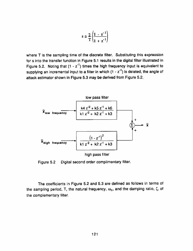
s_=2- TT +

where T is the sampling time of the discrete filter. Substituting this expression

for s into the transfer function in Figure 5.1 results in the digital filter illustrated in

Figure 5.2. Noting that (1 - z"1) times the high frequency input is equivalent to

supplying an incremental input to a filter in which (1 - z1) is deleted, the angle of

attack estimator shown in Figure 5.3 may be derived from Figure 5.2.

Xlow frequency

Xhlgh frequency

low pass filter

k4 z2 + k5 z1 + k6

klz -2+ k2z 1+k3

(1-z") 2

kl z2+ k2z 1 +k3

high pass filter

Figure 5.2 Digital second order complimentary filter.

The coefficients in Figure 5.2 and 5.3 are defined as follows in terms of

the sampling period, T, the natural frequency, o_n, and the damping ratio, _, of

the complementary filter.

121

_'lf

A_hf

low pass filter

k4 z "2 + k5 z"1 + k6

klz "2+ k2z "1+k3

1 -Z "1

klz 2+ k2z "1+k3

high pass filter

-t-i

+

Figure 5.3 Digital angle of attack complementary filter.

T 2 2

K1 = 1 - T_(o n + -_- (.on

T 2 2 2K2 = y (on -

T 2 2

K3 = 1 + T_(O n + -_- (on

T 2 2 T_(o nK4 = 7 (on-

T 2 2

K5 = _ (.On

T 2 2

K6 = T_(o n + -_- (on

5.4 High Frequency Angle of Attack Estimate

As illustrated in Figure 5.4 the angle of attack of the vehicle can be

expressed by the relationship

o_=0-7+o_ (5.1)

122

Ideally, the incremental change in angle of attack, shown as the high

frequency input in Figure 5.3, should be based on the taking the incremental

variation of Equation 5.1:

Ao_= A0 - A7 + Aor., (5.2)

However, as explained previously, Ao¢ is approximated in the ALS

implementation by A0. The effects of this approximation is discussed below in

terms of the two contributions to Ao_that are omitted.

First, the incremental change Aok_ is due to the variation in winds normal

to the velocity vector. This quantity, however, is not measured and its effect is

neglected in the computation of o_. As a result, the estimators response to winds

is dependent on only its low frequency channel which is subject to low pass

filtering. However, by choosing a break frequency, 0%, which is close to the 0

dB crossover frequency of the open loop control transfer function, the effects of

the lag in the load relief response to winds will be reduced. The value of this

break frequency selected for the ALS is 2 rad/sec, which is only a factor of two

below the crossover frequency in the Q(z-limit mode.

Second, the effect of neglecting the contribution of A7 to Ao_ can be

expressed in terms of

A'_ -_-T ":it (5.3)

where T is the control sampling period. The rotation rate of the velocity vector, 4/

, is determined as follows (see Appendix D): First the linear acceleration of the

vehicle normal to the earth relative velocity vector is expressed as

E Fwz = -M_V = T b sin (8- a)+ Tc sin (8- o_)+ Mg cos (7)

- SQC n cos (o_)+ SQC a sin (or) (5.4)

Then, solving for 41yields

123

_/= (T b + T_) sin(s- 8) _-SQC. cos (o_) SQC a sin (a) g cos (y) (5.5)MV MV MV V

UBX

EarthRelativeHorizontal

Figure 5.4 Vehicle orientation parameters.

The flight path angle rate is typically small and does not vary rapidly in Phase

Three. This is shown in Figure 5.5 where the back difference of gamma is used

to calculate a typical _' profile for a no-wind trajectory. The effect of ";/ is to

introduce a small-time varying bias in the estimation of AGHF. If the

complementary filter were a first order filter this i-produced bias would be

transmitted to the estimator output, subject to the low pass filtering. In that case

it might be advisable to employ an approximate computation of ";/to correct the

high frequency input. However, in the case of the ALS where the computation

of 1' is more complicated it appears that a more attractive alternative is to employ

a second order complementary filter which attenuates a slowly varying _' and

eliminates the effects of a constant _. Thus, it is seen that the response of the

estimated angle of attack in Figure 5.3 to a constant A_hf , as might be produced

124

by a constant _/, is obtained by letting z=l, producing a zero contribution to the

estimated angle of attack, _z. Also a constant A_.hf in the discrete signal

implementation corresponds to a constant &if in the continuous signal

representation, in which case the effect of a constant &if on the estimated angle

of attack is given by

" (s) (5.7)_z (s) - s2 . 2_conS + con

2 (xhf

¢J

"0v

0"10

EE

(3

-0.1

-0.2

-0.3

-0.4

-0.5

-0.6

-0.7

-0.830

?:- ?old

I I I I I I I I

40 50 60 70 80 90 100 110 120

Time (sec)

Figure 5.5 Typical _ profile for Phase Three.

which indicates that the contribution to the estimated angle of attack is

well attenuated for frequencies that are well below the break frequency con, and

that the contribution is zero for an input frequency of zero.

In summary, it has been shown that for the second order complementary

filter with the selected break frequency of 2 rad/sec it is possible to employ a

high frequency input of

125

A(Zhf = Ae

It will be recalled that a primary reason for employing the complementary filter

was to make the estimator characteristics primarily dependent on the high

frequency, attitude based input signal in the vicinity of the critical 0 dB crossover

frequency of the Qo_-Iimit mode listed in Table 3.1.

The method of computing the low frequency input to the angle of attack

estimator will now be considered.

5.5 Low Frequency Angle of Attack Estimate

As shown in the flow chart of Figure 5.6, the five step procedure for

computing the low frequency input to the o_estimator first involves determining

an estimate of the acceleration of the vehicle along the yaw axis (UBZ) based

on measurements from the IMU as well as estimates of angular rate and

angular acceleration. The estimated cg acceleration is then employed as an

input to estimating the normal aerodynamic force, F n. Following this, the normal

aerodynamic force coefficient, Cn, is determined from the quotient of the

estimated normal force and the product of the cross-sectional area of the

vehicle, S, and the estimated dynamic pressure, Q. (An improved method for

determining the dynamic pressure based on an air-relative velocity estimate

instead of the usual earth-relative velocity is described in Chapter Six.) The low

frequency estimate of angle of attack is then found by performing a table look-

up procedure, (See Appendix B) based on a table containing pre-calculated

aero-coefficients (Cn) as a function of Mach number and angle of attack. The

resulting low frequency estimate is then passed through a low pass filter to

attenuate unwanted high frequency components and summed with the

corresponding filtered high frequency estimate to yield an estimate of angle of

attack that is valid over a wide range of frequencies.

The derivation for the low frequency estimate of angle of attack in the

pitch plane defined by the body-axis vectors, UBX and UBZ, is as follows.

From Figure 5.7 the acceleration of the center of gravity along the body negative

z axis is given by the equation

126

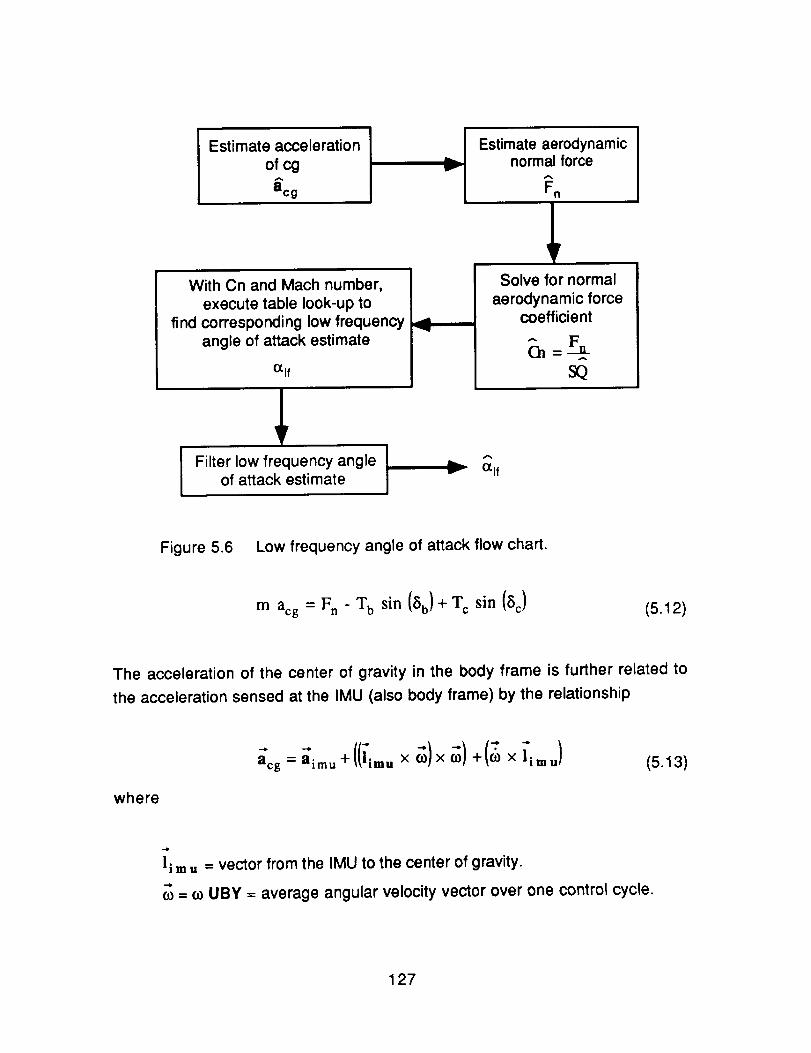
Estimate accelerationof cg

B'cg

With On and Mach number,execute table look-up to

find corresponding low frequencyangle of attack estimate

(Zlf

I Filter low frequency angleof attack estimate

Estimate aerodynamicnormal force

F,

Solve for normal

aerodynamic forcecoefficient

A

SQ

Figure 5.6 Low frequency angle of attack flow chart.

m acs = F n - T b sin (Sb)+T c sin (5c) (5.12)

The acceleration of the center of gravity in the body frame is further related to

the acceleration sensed at the IMU (also body frame) by the relationship

where

!_m u = vector from the IMU to the center of gravity.

_o= o_ UBY = average angular velocity vector over one control cycle.

127

o_ = _ UBY = average angular acceleration vector.over one control

cycle.

The acceleration, a'imt, corresponds to the translation of the vehicle, while the

relative accelerations ((iimu x _)x _)and (_x l"i,,, u) are associated with the

rotation of the vehicle about the center of gravity. The component of acg along

the body negative z axis can be expressed as

acg = aim u + limu =2 sin (13)- lira u d_ cos (13) (5.14)

The angle, 13,defining the location of the IMU as shown in Figure 5.7 is typically

less than 8°. Therefore, using small angle approximations ( sinl_13, cosl_] ),

Equation (5.14) is simplified to

acg = aimu ÷ limu ¢'°2 13 - lim u d_ (5.15)

Therefore, the estimated acceleration of the center of gravity along the

bocly negative z axis is a function of the IMU to cg vector (lirau, 13)as well as the

angular rate and angular acceleration of the vehicle (o_, (o). As discussed in

Chapter Four, the angular rate and angular acceleration of the vehicle are

estimated quantities. From Figure (4.9) it can be seen that the angular

acceleration of the vehicle is available from two separate signal paths. The first

estimate, _1, is derived from the back difference of the estimated angular rate,

and the second, (o2, is the average angular acceleration (over a control cycle)

based on an assumed dynamic model of the vehicle. Both angular acceleration

estimates are corrupted by quantization noise in the measurements of AV and,3. ,3.

A0. The effects of this noise upon the accuracy of r.o1 and (o2 is dependent upon

the filter coefficients chosen for the angular estimation loop. The estimated

average normal aerodynamic force over one control cycle is then obtained by

substituting Equation (5.15)into Equation (5.12).

128

Fn = m (aim u + lira u _2 13-lira u &)+ T b sin (8)- T c sin (15) (5.16)

The normal aerodynamic force is also related to the coefficient of normal force,

Cn, by the relationship

Cn= -_ (5.17)SQ

/

F

aimu

ac(

Figure 5.7

+z

Vehicle Free Body Diagram for determination of Fn.

129

where S is the cross-sectional area of the vehicle, and Q is the estimated

dynamic pressure. Following the estimation of Cn, an aerodynamic table look-

up procedure is employed for estimating the low frequency angle of attack.

These tables list the coefficients of normal and axial force as a function of Mach

number and angle of attack. To determine c¢N the estimated coefficient of

normal force and the current Mach number are employed in a linear

interpolation search. A detailed description of this search procedure is found in

Appendix B. Finally, the estimated low frequency angle of attack estimate is

passed through a complementary low-pass filter and summed with the

corresponding filtered high frequency estimate to produce an estimate of angle

of attack that is valid over a wide range of frequencies.

5.6 Angle of Attack Filter Coefficients

The angle of attack estimator sums a high frequency estimate based on

attitude measurements and a low frequency estimate based on measured 8,

AV, and estimated co and _ through a complementary filter. The high and low

pass filters of the complementary filter are second order. The natural frequency

of both filters, COn, and damping ratio, 4, are important in determining the

accuracy of the angle of attack estimator as well as the control loop stability of

the system. For a system with perfect high and low frequency estimates the

complementary filter would reduce to a unity transfer function. In reality,

however, both high and low frequency estimates contain errors. The extent that

these errors effect the accuracy of the angle of attack estimator and the stability

of the control loop depends in large part to the chosen filter parameters o_n and

4. In determining the appropriate values for these coefficients several

conflicting issues must be considered.

5.6.1 Issues Effecting Choice of Filter Coefficients

For the high frequency path of the angle of attack estimator the issues

are:

130

(I) The attitude signal quantization produces fluctuations in the

measured incremental change in attitude over a control period.

This produces corresponding fluctuations in the estimated angle of

attack, depending on the filter characteristics.

(2) As previously mentioned, the high frequency estimate of angle of

attack does not incorporate the effect of the rotation of the velocity

vector (';/). As a result, the prefiltered high frequency angle of

attack estimate may contain a slowly varying bias. To help

eliminate this bias and its effect upon the accuracy of the angle of

attack estimate a second order high pass filter was employed.

Increasing the crossover frequency of the complementary filter,

reduces the effects of the slowly-varying bias. However, as will be

shown below, increasing this frequency also magnifies the effects

of quantization and modelling errors on the low-frequency

estimate.

For the low frequency path of the angle of attack estimator the issues are:

(I) The low-frequency estimate is a function of the estimated angular

rate and angular acceleration (see Chapter Four). Both of these

signals are effected by quantization errors in measured Ae, and

AV signals. The extent to which these errors effect the low

frequency estimate is a function of the amount of attenuation

present in the low-pass filter. This attenuation level of the filter is a

function of its parameters ((on, t_).

(2) The choice of (on is dependent upon the need to minimize the

adverse effects of uncertainties in the parameters used to estimate

the angle of attack. These uncertainties are not as yet defined for

the ALS. However, it is assumed for the purposes of this thesis

that because of these uncertainties it is desirable to select a (on

value that is lower than the 0 dB crossover frequency of the control

131

loop. This choice of (on prevents the uncertainties from adversely

affecting the frequency response in the critical range near and

above the 0 dB crossover frequency.

The statistical properties of the error in estimated angle of attack are

listed in Tables 5.1 and 5.2 for various quantization levels, assuming that the

angular acceleration estimates employed in the angle of attack estimation are

"3" "?" ^ _2based on (ol and (o2 ,respectively. The values of _1 and and corresponding

o_ estimates were computed from the variables generated in a no-wind

simulation in which true values of feedback variables were employed. The

values of the second order complementary filter parameters used were (on=2

rad/sec and _,=0.8. It will be recalled that

A(ol = angular acceleration estimated based on the back difference

in estimated angular rate.

= angular acceleration estimate based on the measured _V

and 8, with a correction for the bias produced by

mismodeling.

Comparing tabulated values of the standard deviation, _, it is seen that

the use of _2 yields better statistical performance for the largest attitude signal

quantization. However, there is not a drastic difference between the standard

deviations either between the tables or within each table. For the angle of

attack estimator presented in Chapter 8 it was decided to employ _ for the

simulation runs.

132

QUANTIZATION

e

(arc sec)

V

(ft/s)

Mean

(deg)

- Or,True

(3

(deg)

(32

(deg 2)

0 0.0000 7.6xl 0 -2 3.83xl 0 .2 1.47xl 0 .3

3 0.0128 8.9x10 2 1.03x10 1 1.08x10 2

3 0.0320 1.2x10 -2 1.62x10 1 2,63x10 -2

11 0.0128 9.5x10 -2 1.26xl 0 1 1.59xl 0 -2

11 0.0320 1.3x10 1 1.65x10 1 2.75x10 -2

110 4.8x10 -1

Table 5.1

6.97xl 0 -10.0128 4.85xl 01

Effects of quantization in angle of attack error using m1.

QUANTIZATION

e V

(arc sec) (ft/s)

Mean

(deg)

- aTrue

(3

(deg)

(32

(deg 2)

0 0.0000 1.3x10 "1 5.63x10 2 3.17x10 3

3 0.0128 1.2x10 1 1.12x10 1 1.25x10 -2

1.5xl 0 "1 1.63xl 0 1 2.67xl 0 -2

1.2x10 °1 1.12x10 -1 1.25x10 -2

3 0.0320

11 0.0128

110

11 0.0320 1.5x10 1 1.63x10 1 2.67xl 0 .2

1.13x10 -1 1.27x10 -21.2x10 "1

Table 5.2

0.0128

A

Effects of quantization in angle of attack error using co2.

133

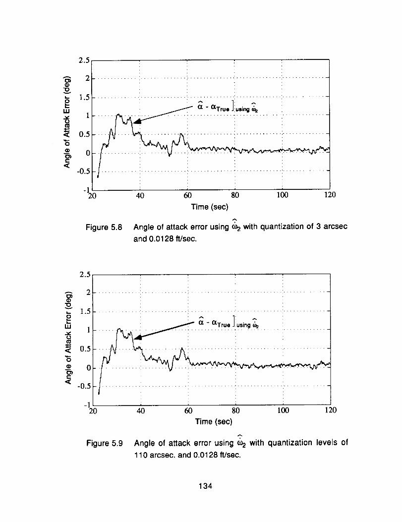
2.5

"10v

LU

O

t-<

1

0.5

0

-0.5

-I20

.............. . .............. i...........................................

1.5 .......................................................................

¢

I I I I

40 60 80 100 120

Time (sec)

Figure 5.8

A

Angle of attack error using m2 with quantization of 3 arcsec

and 0.0128 ft/sec.

2.5

-_ 2"10v

,.. 1.5O

LU 1

:I=< 0.5

0

0

e.-<

-0.5

-120

.......................................... i ............................

............ i .............. i............... i ............................

I | I I

40 60 80 100 120

Time (sec)

Figure 5.9

A

Angle of attack error using o_2 with quantization levels of

110 arcsec, and 0.0128 ft/sec.

134

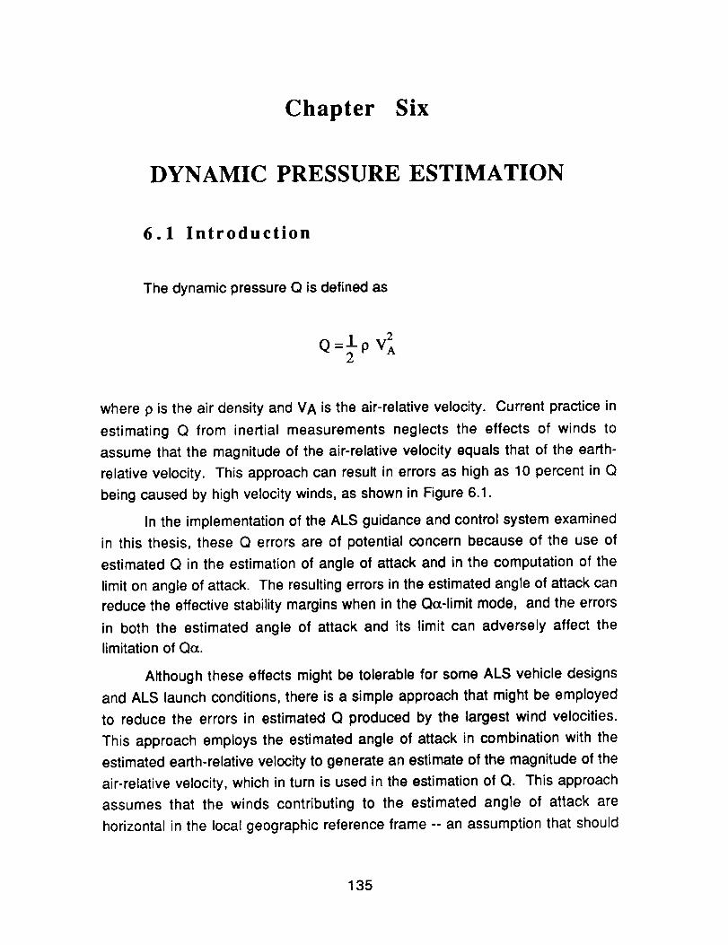
Chapter Six

DYNAMIC PRESSURE ESTIMATION

6.1 Introduction

The dynamic pressure Q is defined as

2

Q=lp VA

where p is the air density and VA is the air-relative velocity. Current practice in

estimating Q from inertial measurements neglects the effects of winds to

assume that the magnitude of the air-relative velocity equals that of the earth-

relative velocity. This approach can result in errors as high as 10 percent in Q

being caused by high velocity winds, as shown in Figure 6.1.

In the implementation of the ALS guidance and control system examined

in this thesis, these Q errors are of potential concern because of the use of

estimated Q in the estimation of angle of attack and in the computation of the

limit on angle of attack. The resulting errors in the estimated angle of attack can

reduce the effective stability margins when in the Qa-limit mode, and the errors

in both the estimated angle of attack and its limit can adversely affect the

limitation of Q(_.

Although these effects might be tolerable for some ALS vehicle designs

and ALS launch conditions, there is a simple approach that might be employed

to reduce the errors in estimated Q produced by the largest wind velocities.

This approach employs the estimated angle of attack in combination with the

estimated earth-relative velocity to generate an estimate of the magnitude of the

air-relative velocity, which in turn is used in the estimation of Q. This approach

assumes that the winds contributing to the estimated angle of attack are

horizontal in the local geographic reference frame -- an assumption that should

135

be most accurate for the very large wind velocities. This assumption limits the

extent to which the Q errors can be reduced, but the possibility of reducing the

largest of the errors makes this approach worthwhile.

00 _ ! ; ;

700 : ........ ' ........ ,... : _.,-r,_..,, .... : ........... : ................. Qbasedon " " .L.Zb, .... J- _,< ..... Earth-relative _ 7_"-_ i "x_, i i

Otto..,,,,=........ velocity. ........ .i/Tq _- __i...... _,. x.......... !............at.,,u_ .......... : ........... :_/--10 % ....... I: -x, ........ : ...........

g 30o................. / ............

° f i200 .......................

]oo .......... i ..

00 20 40 60 80 100 120

Time (sec)

Figure 6.1 Q based on Earth -relative and air-relative velocities using

tail wind Vandenberg #69 wind profile.

6.2 Estimation Procedure

The estimation of Q in this thesis is based (1) on a function of the density

p in terms of the estimated altitude based on a standard atmospheric model and

(2) on the use of the estimated angle of attack to improve the estimation of Q

based on the earth-relative velocity. The relationships employed in (2) are

derived below.

The quantities used to estimate the air-relative velocity are:

136

ft. = (0, _Zpitc h, _'yaw) = estimated angle of attack.

assumed to be zero.

For this thesis _yaw is

V E = inertial earth relative velocity.

BC I = body to inertial transformation matdx

ICu3 = inertial to local geographic reference frame transformation matrix.

An illustration of the vector relationships used to estimate VA is shown in

Figure 6.2. The estimation procedure is as follows:

A

1. Determine the vector U a, by the relationship:

U a = unit (0, _tpitc h, _yaw) (6.2)

A

U a is a unit vector normal to the plane formed by the roll axis of the

vehicle and the air-relative velocity vector. For this thesis there is

no yaw plane motion, therefore

U(x = (0, ], O) (6.3)

, Using small angle approximations compute the total angle of

attack from the relationship

%/-.2 ,-.2_ttot ---- Otpitch + Otyaw (6.4)

137

, Determine the unit vector which defines the orientation of the air-

relative velocity vector in the body frame using the following

relationship based on Equations (6.2) and (6.4):

UAB,d_ = X COS _tot "

where

A

U a x X sin _tot(6.5)

X= (1,0, 0) is the direction of the roll axis in body coordinates.

Since the motion of the vehicle is assumed to be limited to the

pitch plane, Equation (6.5) can be reduced to:

A.o_, = (COS _tot' O, sin _tot)(6.6)

.

A

Transform the unit vector UAmo=' from the body frame to the local

geographic coordinate frame by the relationship:

A I B'"

UAL¢; = C LG C I UABod, (6.7)

where

B

C I = a body frame to inertial frame transformation matrix and

iCI_ = an inertial frame to local geographic frame transformation

matrix.

138

I BThe product of CLG C I is equivalent to a single transformation

from the body frame to the local geographic frame.

, Transform the earth relative velocity vector, VE, from the body

frame to the local geographic frame and unitize the resulting

vector.

"" I B _"

VEc 6 = C LG C I YEs,,, (6.8)

(6.9)

. Assuming that the wind velocity is horizontal so that the difference

between the vertical components of VF. and V A is zero, determine

the magnitude of VA using the relationship below:

[;" ^ ^ Jz component of E UELo - VA UA L Local

(Z component of wind) = 0

Geographic =Frame

(6.1o)

Solving for VA in Equation (6.10) yields the final result:

UALo component (6.11 )

This estimate of air-relative velocity magnitude is then used to

compute dynamic pressure by the relationship

139

(6.12)

HORIZONTAL PLANE

V w is in horizontal plane

LOCAL GEOGRAPHIC_

HORIZONTAL PLANE

VERTICALPLANE

Figure 6.2 Vector relationships for air-relative velocity estimator.

6.3 Effects of Improved Air-Relative Velocity

Estimation

Using the derivation from the previous section, two simulations were run

to test the accuracy of the Q estimation procedure. Each test was begun at the

end of Phase Two which corresponds to the point when acceleration

direction/angle of attack steering begins. Two tail wind profiles, Vandenberg

140

#70 and Vandenberg #69, were chosen as worst cases. A discussion of the

characteristics of each profile is presented in Appendix G.

Since dynamic pressure is proportional to the square of air-relative

velocity, a measure of the effects of the air-relative velocity estimation on the

estimated dynamic pressure can be obtained by computing a ratio (r) between..-.2

the error in the square of estimated air-relative velocity, e(V A), and the square

2of the true air-relative velocity, VA- ie.

(;)c V V A - V A V Ar= = - I

2 2 2VA VA VA (6.13)

A plot of the ratio, r, is given in Figures 6.3 and 6.4 for the two wind

profiles.

The shape of both curves is very similar. Both show a large initial

transient excursion followed by a "tailoff" period after 100 sec. in which the error

in Q increases exponentially. The peak error in Q for both trials is

approximately 2.25%. This error occurs at the beginning of the estimation

procedure and is due to the initial transient errors associated with the angle of

attack estimator. The reduction in accuracy in the estimate of dynamic pressure

shown in the tailoff portion of the curves is a result of the degradation in the

angle of attack estimate as the dynamic pressure approaches zero.

141

0.025

0.02

0.015

0.01

r0.005

0

-0.005

-0.01

-0.01530

Figure 6.3

h. • .......

J............i............._,..0_0o..0i,.0....i.......i......

I I ! i I | I I

40 50 60 70 80 90 100 110 120

Time (sec)

Error ratio relating estimated and true air-relative velocities for

Vandenberg wind profile #70.

0.025

0.02

0.015

0.01

r 0.005

0

-0.005

-0.01

-0.01_0

Figure 6.4

m ,

-f ..... i ....... i ....... i ..... vandeni:xJri piOfile #69 ..... i ....... ......

I I I I I | | I

40 50 60 70 80 90 100 110 120

Time (sec)

Error ratio relating estimated and true air-relative velocities for

Vandenberg wind profile #69.

142

Chapter Seven

TRAJECTORY DESIGN

7.1 Introduction

The guidance commands issued for the first three phases of flight are

specified prior to launch. These commands are functions of time and determine

the desired path or trajectory that the vehicle will follow until the predictive-

adaptive powered explicit guidance takes over. Deciding which trajectory is

most appropriate for the given mission is the objective of the trajectory design

process. The shape of the trajectory is determined by specified objectives and

constraints. In general, the objective is an end condition and represents some

desired terminal state. The constraint is a boundary that limits and/or restricts

the shape of the trajectory. The QO_limit, for example, is one physical constraint

on the trajectory.

In previous work by Michael Corvin for the single-stage-to-orbit (SSTO)

Shuttle II vehicle, the primary mission objective was to maximize the terminal

mass of the vehicle. By maximizing the terminal mass more fuel was available

for any post boost maneuvers. In addition, by minimizing the required fuel

needed to achieve orbit, payloads of higher weight could be lifted. This

objective of maximizing the terminal mass is also assumed as the primary

mission objective in this thesis.

As previously mentioned in Chapter 2, the trajectory of the vehicle is

divided into four phases. The trajectory design program is employed to

determine the parameters which define the shape of the trajectory in the first

three phases. Phase Four employs a close to optimal predictive-adaptive

guidance whose trajectory depends on the initial conditions provided by the

combined effects of the first three phases.

The design program defines the trajectory shape in the first three phases

in terms of

143

(I)

(2)

(3)

The altitude the vehicle is to reach at the end of the vertical rise

from the launch pad in Phase One.

The function describing the desired attitude rate versus time in

Phase Two.

The parameters of an angle of attack profile defining the shape of

the trajectory in Phase Three for the initial conditions provided by

Phase Two.

Although the altitude required for the vertical rise of (1) can be varied to

optimize the shape of the boost trajectory, it was decided to clamp this required

altitude at 400 ft.

Two alternative time functions will be considered for the rapid pitchover

of (2). These functions differ in their ability to determine the end conditions for

this flight phase. The functions and their effects on end conditions will be

discussed in Section 7.2.

Three parameters used to define the angle of attack profile of (3) will be

described in Section 7.3. It should be noted that although it is convenient to

design this portion of the trajectory for Phase Three in terms of the angle of

attack profile, the in-flight guidance for this flight phase employs an estimated-

acceleration-direction profile corresponding to the angle of attack profile as the

command signal.

The trajectory design process involves iteratively adjusting the

parameters and functions for the three initial phases to produce a maximum

mass at the end of Phase Four. These adjustments must pay particular

attention to (a) the need to produce final conditions for Phase Two that are

consistent with the initial angle of attack and attitude rate desired at the

beginning of Phase Three and (b) the need to have an acceleration direction at

the end of Phase Three that approximately matches the acceleration direction

that will be commanded by the predictive-adaptive guidance in Phase Four.

Section 7.4 provides a brief description of the predictive-adaptive

guidance employed in Phase Four and of the orbital goals employed in the

application of this guidance. The acceleration direction command supplied by

this guidance is generated as a function of time by a "linear tangent guidance

144

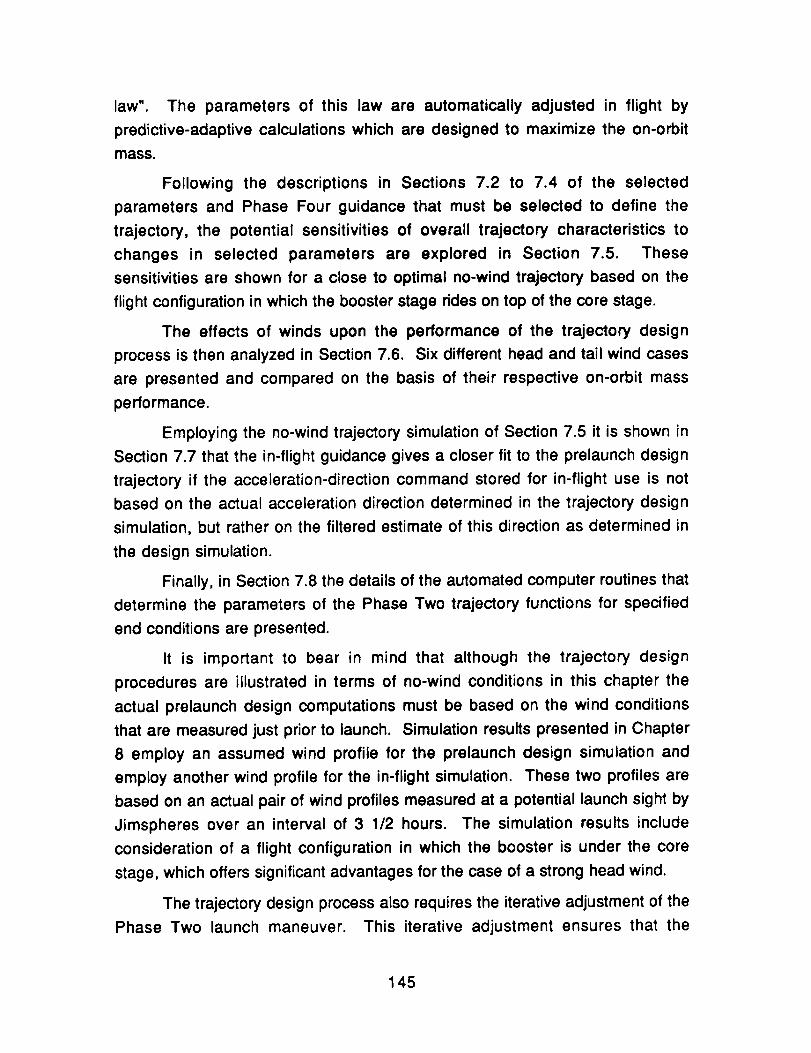
law'. The parameters of this law are automatically adjusted in flight by

predictive-adaptive calculations which are designed to maximize the on-orbit

mass.

Following the descriptions in Sections 7.2 to 7.4 of the selected

parameters and Phase Four guidance that must be selected to define the

trajectory, the potential sensitivities of overall trajectory characteristics to

changes in selected parameters are explored in Section 7.5. These

sensitivities are shown for a close to optimal no-wind trajectory based on the

flight configuration in which the booster stage rides on top of the core stage.

The effects of winds upon the performance of the trajectory design

process is then analyzed in Section 7.6. Six different head and tail wind cases

are presented and compared on the basis of their respective on-orbit mass

performance.

Employing the no-wind trajectory simulation of Section 7.5 it is shown in

Section 7.7 that the in-flight guidance gives a closer fit to the prelaunch design

trajectory if the acceleration-direction command stored for in-flight use is not

based on the actual acceleration direction determined in the trajectory design

simulation, but rather on the filtered estimate of this direction as determined in

the design simulation.

Finally, in Section 7.8 the details of the automated computer routines that

determine the parameters of the Phase Two trajectory functions for specified

end conditions are presented.

It is important to bear in mind that although the trajectory design

procedures are illustrated in terms of no-wind conditions in this chapter the

actual prelaunch design computations must be based on the wind conditions

that are measured just prior to launch. Simulation results presented in Chapter

8 employ an assumed wind profile for the prelaunch design simulation and

employ another wind profile for the in-flight simulation. These two profiles are

based on an actual pair of wind profiles measured at a potential launch sight by

Jimspheres over an interval of 3 1/2 hours. The simulation results include

consideration of a flight configuration in which the booster is under the core

stage, which offers significant advantages for the case of a strong head wind.

The trajectory design process also requires the iterative adjustment of the

Phase Two launch maneuver. This iterative adjustment ensures that the

145

transition from Phase Two, to Phase Three is "smooth'. Two different launch

profiles are presented, both of which are based on time functions of

commanded pitch rate. A launch design program was written to automate the

iterative launch design process.

The trajectory design technique is implemented using the main 6 DOF

simulation. Although the parameters of the angle of attack profile were

optimized, no attempt was made to show that this particular formulation of an

alpha based trajectory was the best choice.

7.2 Phase Two Functionalization

The choice of the functionalization to generate the commanded attitude

rate in Phase Two is a crucial part of the trajectory design process because of

(1) the major role played by the rapid pitchover in Phase Two in determining the

overall trajectory shape and (2) the importance of achieving a smooth transition

from the rapid pitchover of Phase Two. This functionalization must provide the

flexibility needed to achieve at the end of Phase Two the value of angle of

attack required at the beginning of Phase Three, with a final attitude that is

compatible with the rate required initially in Phase Three.

This thesis investigates two different launch profiles of commanded attitude

versus time for Phase Two. Both algorithms employ a smooth sinusoidal pitch

rate command. The first launch profile was developed by Michael Corvin for the

single-stage-to-orbit Shuttle II launch system. This method is shown in Figure

7.1. The second launch profile illustrated in Figure 7.2 is similar to the first

except that the commanded pitch rate is held constant throughout the second

half of the maneuver. Two parameters are necessary to define the launch

profiles. The first, Tk_, is the desired duration of Phase Two, and the second,

Q, is a rate equal to half the maximum pitch rate. Determination of these

parameters is achieved by a launch design program which iteratively adjusts

Tkick to obtain the desired end-of-maneuver state necessary for a smooth

transition to Phase Three. A discussion of the automated launch design

process is found in section 7.6.

The initial trajectory shaping studies were performed successfully using

only the sinusoidal launch maneuver. However, although the profile provided a

146

smooth transition in angle of attack it was observed that during the transition

from Phase Two to Phase Three the flight controller would command a large

step in commanded nozzle deflection which produced a large increase in

attitude rate. This large increase in pitch rate was required so that the vehicle

could follow the initial constant angle of attack profile (o_1) commanded in

Phase Three. This sudden increase in pitch rate is undesirable for the following

reasons:

2_

{deg_e ,s---d_-,

0

Phase Two Start

1 ITKick 0 <_t _<TK_

I v

TKick -= (Tphase Three Start-

Time (see) " Tphase Two Start )

Figure 7.1 Phase Two command profile with sinusoidal pitch rate

(1) First, any large increases in commanded attitude rate could cause

the core and booster nozzles to rate limit. (For the ALS it was

decided to limit the nozzle rate to 10°/sec).

(2) Any large changes in the attitude of the vehicle adversely affects

the performance of not only the angular rate and angular

acceleration estimates, but also the angle of attack estimate.

To help remove the effects caused by the large change in commanded

angular velocity, the new Phase Two launch profile described in Figure 7.3 was

developed. This launch profile involves an initial sinusoidal pitch rate launch

maneuver followed by a non-zero terminal pitch rate. The shape of this profile

enables the launch designer to specify not only the terminal attitude and

duration of Phase Two, but also the desired terminal attitude rate. Although this

147

adds a degree of freedom to the launch design process it does not further

complicate the procedure for determining the suitable launch design

parameters. A detailed description of this launch maneuver is found in section

7.6.

2£4-

0

(_= _(1-COS(TTrans2_ t))]0<-

I

Ttrans

Phase Two Start

Time (see)

t < TTran =

1

k

I

TKick -'- (Tphase Three Start

" Tphase Two Start )

Figure 7.2 Phase Two command profile with constant terminal pitch

rate.

7.3 Phase Three Functionalization

As illustrated in Figure 7.3 the angle of attack profile for Phase Three is

defined in terms of the following three parameters that may be adjusted within

vehicle design constraints to maximize the on-orbit mass:

(1) An initial angle of attack, (_1, which is maintained until the product

Qoh reaches a specified limit.

(2) A Q(_limit which is followed until the resulting o_(with decreasing Q)

increases to a specified final value.

(3) A final value of angle of attack, o_2.

The degree to which these three parameters can be varied to optimize

the boost trajectory is limited by

148

(I)

(2)

(3)

The degree of flexibility in Phase Two to produce the desired initial

conditions in Phase Three

The required margin of safety between the Qo_limit and the vehicle

structural limit on QoL

The need to produce a terminal a that is compatible with the initial

guidance commands generated in Phase Four.

o_

o_1

o_2

III

II

I

ID_B,_ mDBm

Q_ limiting begins

_ Qc_ = constant = Q(Z.limit

_J / Qo: limiting ends

I!I

_ _ TimeEnd of Start of

Phase Two Phase Four

Figure 7.3 Trajectory shaping angle of attack profile.

The trajectory shape in and beyond Phase Three is strongly influenced

by the depth of the Qo_ bucket in Figure 7.3, as determined by the selection of

the QO_limi t for the trajectory design. The value of this limit must be well below

the assumed structural limit of 3,500 Ibs deg/ft 2. For the ALS vehicle a margin

between this structural limit and the trajectory design limit is required so that the

vehicle will have the ability to tolerate transient excursions in Q(z during periods

of Qe_ limiting. Even in no-wind simulations, Qo_ typically exceeds the Q_limit by

as much as 80 Ibs deg/ft 2. Consequently, to provide a safe design margin it was

decided to set Qo_lim_at 3,000 Ibs deg/ft 2.

149

7.4 Predictive-Adaptive GuidanceFour

for Phase

The predictive-adaptive Powered Explicit Guidance (PEG) program is

employed both in flight and in the trajectory design calculations for Phase Four.

In both cases the guidance program is employed every six seconds to adjust

the parameters of a "linear tangent guidance law" that generates the

commanded acceleration direction as a function of time. This guidance law is

expressed as

tan OAc = K o + (t -t o) K 1

where OAc is the commanded acceleration angle and Ko, K1, and to are the

adjusted parameters. The guidance program solves analytical relationships to

predict the amount of propellant required to reach specified orbital conditions

from the current vehicle state. Using this analytical prediction the program

adjusts the linear tangent function parameters to minimize the propellent

required, and thereby maximize the on-orbit mass.

In both the trajectory design calculations and the in-flight guidance

calculations the analytical predictions of PEG are simplified by neglecting the

effects of the aerodynamic forces. Since Phase Four is initiated in the upper

atmosphere this simplifying assumption results in small prediction errors in the

beginning of Phase Four which steadily reduce as the vehicle emerges from the

atmosphere. For the purposes of this thesis investigation it was decided to

simulate the response of the vehicle to PEG only up to the point of staging in

both the cut-and-try design simulations and the final in-flight simulations for

performance evaluation. The analytical relationships of PEG are then used to

predict the on-orbit mass resulting from the post-staging boost trajectory. In his

Shuttle II studies, Corvin found that the use of such analytical predictions, in lieu

of actual simulations to the end of boost, did not significantly degrade the

trajectory optimization.

150

Along with the predicted on-orbit mass the PEG algorithm also calculates

the commanded attitude change at the transition to Phase Four. This variable

was useful since it provided insight into the shape of the trajectory. Based on

experience, the magnitude of the commanded attitude change indicated

whether the trajectory was too low or high with respect to the sought after

optimal one. Generally, those trajectories which had minimum commanded

attitude changes at PEG also had correspondingly high values of terminal on-

orbit mass.

The orbital objective used in all PEG calculations in this thesis is based

on the following two conditions

(1) The perigee of the vehicle is 80 Nmi. and

(2) The velocity (horizontal) of the vehicle is large enough to achieve

an apogee of 150 Nmi. This velocity is determined from the

relationship

V orbit =_rp el

rap + rpe

1/2

where I_ is the gravitational constant, rap is the apogee, and rpr is

the perigee. 1

7.5 Trajectory Parameter Sensitivity Analysis

The effects of adjusting the various design parameters for both Phase

Two and Three are illustrated in Figures 7.4 through 7.19. For each design

parameter, plots of flight path angle (1,) and attitude (0) are provided. Each plot

contains three curves. A solid line represents the launch design profile for the

1 Battin, Richard H., An Introduction to the Mathematics and Methods of

Astrodynamics.1987. New York: AIAA Educational Series. (pp 116).

151

selected "optimal" value of the given launch design parameter. Dashed curves

represent the the response of the vehicle to small perturbations in each of the

launch design parameters. The results of this perturbation analysis are also

shown in Table 7.1. For each separate launch maneuver an "optimal" set of

trajectory design parameters was first obtained. These results are presented in

italics and are listed as "Nominal" in the Run Number column. In Table 7.1

Launch Profile #1 corresponds to the sinusoidal launch maneuver illustrated in

Figure 7.1, while Launch Profile #2 represents the non-zero terminal pitch rate

launch maneuver shown in Figure 7.2. For each simulation the terminal on-

orbit mass (as predicted by the PEG algorithm), as well as the pitch attitude

change at PEG was also recorded. In addition, a sensitivity quotient which

measured the effect of perturbations in the launch design parameters to losses

in the predicted optimal on-orbit mass was also calculated. This performance

measure was obtained by using the general expression

S.Q. = [On-orbit MasS]Nominal- IOn-orbit iaSS]p_rturbatio n[Trajectory Parameter]Nomina j -[Trajectory Parameter]perturb=_n

(7.1)

where the TrajectoryParameter iseitherel,Of,al, 02, orthe Qo_irn_t.

The Nominal run foreach launch profilewas based on a minimizationof

the change in pitchattitudeat transitionto PEG. As shown in Table 7.1 most

trialswhich had largervalues of "A pitch"at PEG also had smaller predicted

terminalon-orbitmasses. The process of minimizingA pitchat PEG, however,

did not always guarantee an optimalon-orbitmass. In one case (Run Number

14) an additional6 slugs of mass was achieved despite a largertransitional

value of A pitch.

For both launch profilesthe variationof the Q(Xlimit had littleeffectupon

the shape and predictedon-orbitmass ofthe trajectory.This was also true for

variationsin o_I. For c_2 itwas noted that small negative deviationsfrom the

nominal case caused the vehicleto pitchover rapidlytowards the latterhalfof

Phase Three. Consequently, the requiredattitudechange at transitionto PEG

was quitelargeforboth launch maneuvers (14.1°forLaunch Phase 1 and 15.2°

forLaunch Phase 2) and the resultingterminalmass was lessthan optimal as

demonstrated by the high sensitivityquotients.

152

In addition to the variables responsible for defining the angle of attack

profile (0_1,0_2, Qoqimit), the effects caused by perturbations in the launch

maneuver parameters (ef, ef) was also investigated. For the sinusoidal launch

maneuver, the desired terminal launch attitude proved to be the most sensitive

variable. For run 4, for example, a variation of only -0.06 ° from the nominal

case caused the vehicle to pitch over rapidly prior to entering Phase Four.

For launch profile 2, the desired terminal attitude rate provided the

largest changes in the terminal mass. In one instance a variation of only

-0.1°/sec caused the predicted terminal mass to decrease by 97 slugs from the

nominal case. However, despite this large sensitivity quotient the effect on the

shape of the trajectory was minimal as evidenced by the small commanded

change in pitch attitude at PEG transition.

7.5.1 Sensitivity Analysis Plots

8O

¢D"O

EE

70

60

50

40

30

20

100

; o i ,;3ooo i

........... ! ........... ! ...... _'___""_" ! ........... !!/ .........Qc_limit =3250!...........

........... i ........... : .......... '. ......... _%. '"",._" : .......... -I,/

20 40 60 80 100 120

Time (sec)

Figure 7.4 Sensitivity of gamma to Qo_ limit for a non-zero terminal

pitch rate maneuver.

153

Run Launch Of ()f a 1 o_2 QO.limit Terminal A pitch Sensitivity

Number Profile (deg) (dog/ (deg) (deg) (Ibdeg/ Mass at PEG Quotient

sec) ft2) (slugs) (deg) S.Q.

Nominal 1 80 11.1 4.5 3000 12167 0.48

1 1 80 11.1 4.5 2750 12164 4.72

2 1 80 11.1 4.5 3250 12153 -3.46

3 1 83 11.1 4.5 3000 12122 -6.95

t t

4 1 79.94 11.1 4.5 3000

5 1 80 10.9 4.5 3000 12143 -4.48 120.0

6 1 80 11.3 4.5 3000 12153 7.93 -70.0

7 1 80 11.1 2.5 3000 12039 14.05 64.0

8 1 80 11.1 6.5 3000 12156 -6.60

Nominal 2 84.5 -0.5 9.5 4.0 3000 12159 0.32

9 2 84.5 -0.5 9.5 4.0 2750 12159 5.33

10 2 84.5 -0.5 9.5 4.0 3250 12141 -3.48 -.072

11 2 81.5 -0.5 9.5 4.0 3000 12160 6.59 -.333

12 2 87.5 -0.5 9.5 4.0 3000 12114 -6.42 -15.0

13 2 84.5 -0.5 9.3 4.0 3000 12142 -3.06 85.0

14 2 84.5 -0.5 9.7 4,0 3000 12165 4.08 30.0

15 2 84.5 -0.5 9.5 2.0 3000 12000 15.21 79.5

16 2 84.5 -0.5 9.5 6.0 3000 12139 -8.06 -10.0

17 2 84.5 -0.4 9.5 4.0 3000 12062 -10.87 -970.0

18 2 84.5 -0.6 9.5 4.0 3000 12100 -7.82 590.0

Table 7.1 Trajectory shaping results. * Trajectory did not reach PEG.

.012

-.056

-15.0

-5.5

154

I00

"Dv

t-l--

8O

6O

4O

2O

00

........ __ ....... : ...... 0o_i =30oo.... : ...........

...........:...........:........"..__,-..../:....o_,._=3250.....

..........._........._._ .....i........'.___. _..........:,,,." : " --_.,,.

Ooclimit:= 2750 : _:" _ -_ _ """

i i L I i

20 40 60 80 lO0 120

Time (sec)

Figure 7.5 Sensitivity of theta to Qa limit for a non-zero terminal pitch

rate maneuver.

8O

_- .........:......nominal.= 84.5-..:...........

i /i i \ 'i_ . i i/

....:OFina I = 81 3; _ "_., -., _. -, ""

' 8o ' ?o40 60 lO0

7O

"-" 6OC_

"10v

E 5OE

(.9 4O

3O

2O0 2'0

Time (sec)

Figure 7.6 Sensitivity of gamma to terminal launch theta for a non-zero

terminal pitch rate maneuver.

155

90

80

70

O_60

"0v

50¢.-1-

40

30

200

...... .:. .......... : .... nominal 84.5 ..... : ...........

_: ...... _:............_ °F!_,,,87_5.................i....... / /.

i i z _" " -_'_-2 ". :

.......... : .......... OEmal-. 8...5..: ........... : ........... :..... _.....

I I I I I

20 40 60 80 100 120

Time (sec)

Figure 7.7 Sensitivity of theta to terminal launch theta for a non-zero


80

........... : ...... _'_ ": ......................... o..............._. : ctl = 9.3 .

...................... : ........ : .......... o.:1= 9.5 _....

i i i i N_..,.................................... "_ '.-4, .... -_. " "

I I

20 4'0 60 8'0 100 120

?0

.-. 60O)

"0

50EE

L9 40

30

200

Time (sec)

Figure 7.8 Sensitivity of gamma to o_1 for a non-zero terminal pitch rate

launch maneuver.

156

9O

8O

?0

60"10

50t-I---

40

3O

200

"_ " ! al = g.3 ° !

........... :............ :...,_._, ..... :i i "_" . i o• al = 9.5

........... i ........... i ......... _._ .......... i ........... i ..........

........... i ........... ; .......... ; ..... "_- >..;..- ;

...... _.-.....-'_._.. _ ..........

........... i ........... i ........... i ........... ; ...... ", _

I I | I I

20 40 60 80 lO0

Time (sec)

120

Figure 7.9 Sensitivity of theta to ¢zl for a non-zero terminal pitch rate

launch maneuver.

8O

?0

c_ 60

"10v

t_E 50E

(.9 40

30

2O I

0 2O

i : : 02=4 ° :i\ i =°o

iii i!....................... 02=2° .......................... ' '< _ :-- "-L-

40 60 80 100 120

Time (soc)

Figure 7.10 Sensitivity of gamma to variations in 0_2 for a non-zero

terminal pitch rate launch maneuver.

157

90

80

?0

v

50e-

i--

40

3O

200

i : i o2-4 ° i i

.......... i,_ i 60 ..........

........... ; ........... ; ........... . ..,,, ..... ; ......... ; ...........

I -

i i i i i •

20 40 60 80 100 120

Time (sec)

Figure 7.11 Sensitivity of theta to variations in ct2 for a non-zero


8O

_,.,, pitchrate -- i0.4

........................... Ntchral .... ........................... "_

i

2'0 4'0 60 8'0 1(_)0 120

Time (sec)

7O

6O

5O

4O

3O

2O0

Figure 7.12 Sensitivity of gamma to variations in terminal pitch rate for a

non-zero terminal pitch rate maneuver.

158

9O

8O

?0

¢:7)60

"0v

50e--

I-

40

3O

200

.......... : ........ _'": ...................................i_. ! pitchrate = -0.4 i;...........

..................... ........... .......:...........

..... pitchr_ --_'.*_._, ................

i i i i i

20 40 60 80 100 120

Time (see)

Figure 7.13 Sensitivity of theta to variations in terminal pitch rate for

a non-zero terminal pitch rate maneuver.

8O

7O

._.60¢7)

"10"---" 50

EE 40

L9

3O

2O

100

Qailimit = + 3250

: : : Qct limit:= + 3000 :

i i _-/-_.i '. .... i lily: ........ ii /.....................................; ........ ; ........ ; ...... .N-', ....... ; .............. ; ........ ; .......

. . • .'% _'x. , .

_'_'__ _ Transfer• i i i _, ,,_

/

........ :... Q_.lin_t.; _+2750 ........ : ........ : ........ [_ "---_ . :.2......1

i i i 1 i i i

20 40 60 80 100 120 140 160

Time (see)

Figure 7.14 Sensitivity of gamma to Qoc limit for a sinusoidal pitch rate

maneuver.

159

9O

80

7O

o_6oQ)

"10v

t_ 50(Dt--

40

3O

20

100

: i i i Q(xlirnit=_3250

i i T _'"- [ i

L '!.=.-+,.........../ :l20 40 60 80 100 120

Time (see)

Figure 7.15 Sensitivity of theta to Q_ limit for a sinusoidal pitch rate

maneuver.

80

7O

6O¢7)

50

EE 40

(.930

2O

100

_. • al = 11.1° •

...... __..i 57_-_.: ........ / ...... _........ _1=113' ........

i ........ i 2_ _NI "\ i i . i

_ _ __ % '4 " i _ ' _m m m _ PEG. -

[ i i i i i i

20 40 60 80 100 120 140 160

Time (see)

Figure 7.16 Sensitivity of gamma to czl for a sinusoidal pitch rate launch

profile.

160

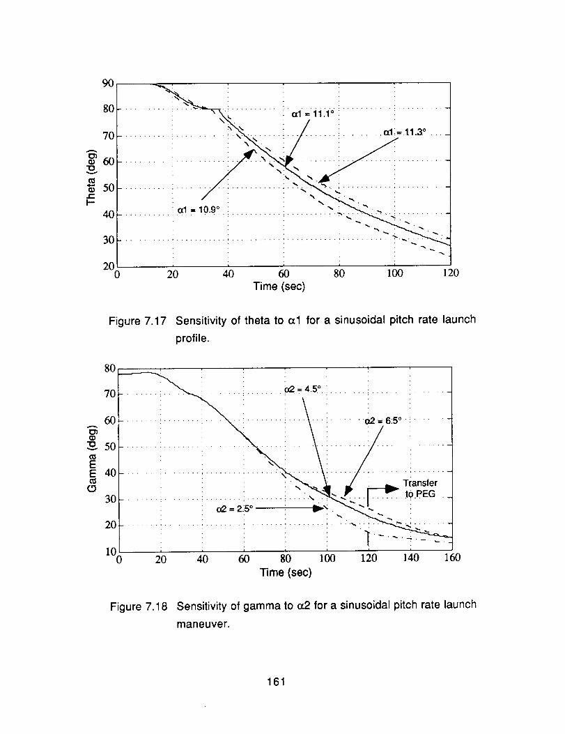
9O

8O

?0

60"10v

50t--I.-

40

3O

200

.-._ .

• %,_

i .......... i ........... __2 ........ % ......... i .......... i ...........

_ ........./ .............-,__

.......... : ........... : ........... : ........... : ........... f._...

i i i i i

20 40 60 80 100 120

Time (sec)

Figure 7.17 Sensitivity of theta to 0_1 for a sinusoidal pitch rate launch

profile.

8O

7O

6O

50

EE

(.9

i i i 4 ° i• . ix2= .5 ...... : ................

40 ....... ! ........ ! ........ ! ....... '_ ....... ! ....... ! ........ : ........Transfer

30 ___-!-.'r _OPEG_

............................................i_:10 .......

0 20 40 60 80 100 120 140 160

Time (sec)

Figure 7.18 Sensitivity of gamma to 0_2 for a sinusoidal pitch rate launch

maneuver.

161

A

Q)"10v

J_I--

90

80

70

60

50

40

30

200

....... _ ........ : ........ -oi4.s, ....... :............

.......... _ --_ ' " •! .......... !\ ....... !-,e =e:so -

• _.

i i i i i

20 40 60 80 100 120

Time (sec)

Figure 7.19 Sensitivity of theta to c¢2for a sinusoidal pitch rate

launch maneuver.

7.6 Effect of Winds on Trajectory Design

In Section 7.5 the effects of adjusting the launch design parameters upon

the shape and performance of the trajectory in a no-wind environment was

analyzed. In order to better understand the effects of winds upon the trajectory

design, a different study was conducted in which the on-orbit mass of the

vehicle was optimized in a wind environment. As shown in Table 7.2, six

different cases were simulated for trajectories ending at staging (= 160 sec after

ignition). For each case a different combination of wind speed and direction

was employed. The wind speed was determined by scaling the stored wind

magnitude of the Vandenberg #69 profile (see Appendix G). In Table 7.2 the

scaling is represented as a percentage of the total wind magnitude. Because

this thesis study is limited to the pitch plane, only head and tail wind directions

were simulated.

For each case a separate set of optimal launch design parameters

corresponding to the sinusoidal launch maneuver was first obtained. The on-

162

orbit mass of the vehicle was optimized by adjusting the launch design

parameters such that the change in pitch attitude at the transition to PEG was

minimized. The prediction of on-orbit mass was determined by the PEG

algorithm at staging. As shown in Table 7.2 the required attitude, el, and angle

of attack, (xl, are larger for the head wind cases. The larger angle of attack

values are primarily due the contribution of winds, while the higher attitude

values are necessary to provide the vehicle with a loftier initial trajectory since

at later times (during Q(z limiting) the trajectory of the vehicle is depressed.

In addition to having a significant impact upon the chosen optimal launch

design parameters, the magnitude and direction of winds also effects the on-

orbit mass of the vehicle. As shown in Table 7.20 larger tail winds increased

the on-orbit mass of the vehicle. Comparing the two 100% head and tail wind

cases it can be seen that the on-orbit mass of the vehicle increased by 71.4

slugs when flying with a tail wind. In addition, the on-orbit mass is linearly

correlated to the wind magnitude. This is illustrated in Figure 7.20 where the

on-orbit mass is plotted against the scaled wind magnitude.

Wind Profile

Magnitude

(% of #69)

Wind Profile

Direction

40

Of

(deg)

Tail Wind

(zl

(deg)

82.95

(z2

(deg)

9.00

pitch

@ PEG

(deg)

Mass

On-orbit

(slugs)

100 Head Wind 87.95 15.30 4.0 0.12 12121.1

60 Head Wind 85.60 13.70 4.0 0.27 12137.9

40 Head Wind 84.90 12.80 4.0 0.13 12145.1

100 Tail Wind 82.75 5.75 4.2 0.00 12192.5

60 Tail Wind 82.75 8.00 4.2 0.04 12182.3

4.2 -0.09 12175.7

Table 7.2 Effect of winds on trajectory parameters and on-orbit mass.

163

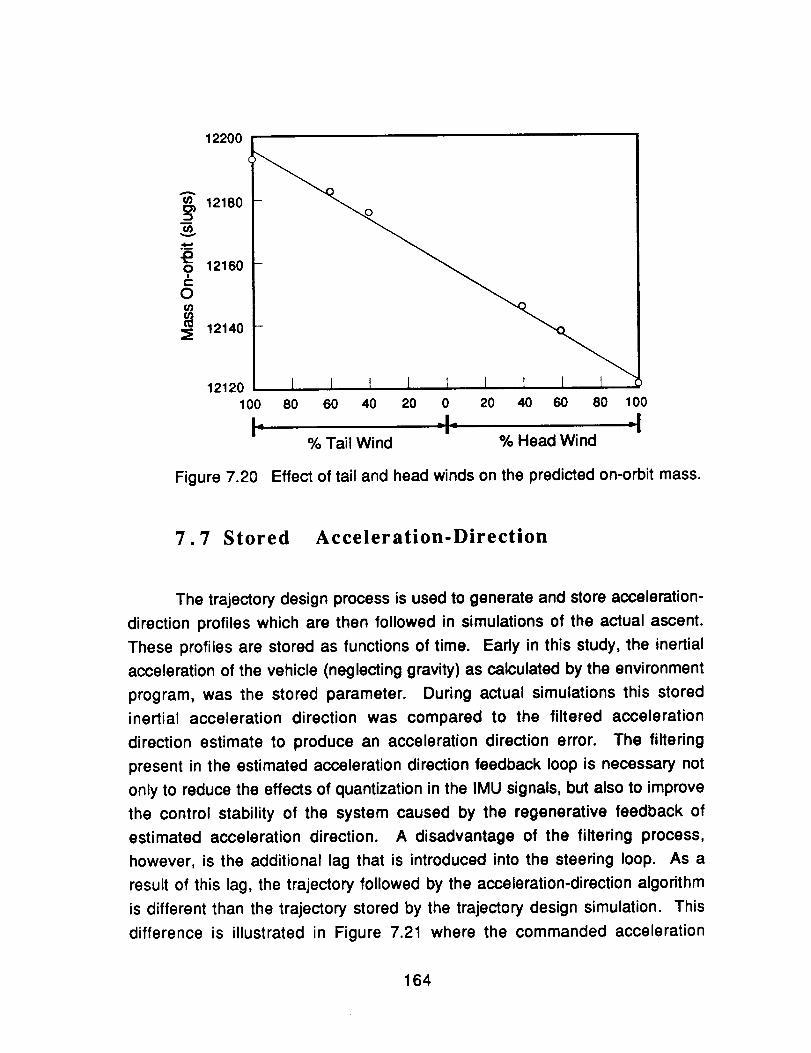
12200

121803

t29 12160C

0

12140

12120

100

I I I I 1 I l I l80 60 40 20 0 20 40 60 80 100

__L J% Tail Wind % Head Wind

Figure 7.20 Effect of tail and head winds on the predicted on-orbit mass.

7.7 Stored Acceleration-Direction

The trajectory design process is used to generate and storeacceleration-

direction profiles which are then followed in simulations of the actual ascent.

These profiles are stored as functions of time. Early in this study, the inertial

acceleration of the vehicle (neglecting gravity) as calculated by the environment

program, was the stored parameter. During actual simulations this stored

inertial acceleration direction was compared to the filtered acceleration

direction estimate to produce an acceleration direction error. The filtering

present in the estimated acceleration direction feedback loop is necessary not

only to reduce the effects of quantization in the IMU signals, but also to improve

the control stability of the system caused by the regenerative feedback of

estimated acceleration direction. A disadvantage of the filtering process,

however, is the additional lag that is introduced into the steering loop. As a

result of this lag, the trajectory followed by the acceleration-direction algorithm

is different than the trajectory stored by the trajectory design simulation. This

difference is illustrated in Figure 7.21 where the commanded acceleration

164

direction is plotted along with the filtered acceleration direction estimate as well

as the actual acceleration direction of the vehicle. As shown the filtered

acceleration-direction lags the commanded acceleration-direction by a

considerable amount. To eliminate the errors associated with the additional

lag, it was decided to store the filtered acceleration-direction during the

trajectory design simulations instead of the actual inertial acceleration-direction.

6

o_ 5"10v

¢-O

.i

15 4

.m

E3t-O 3

.m

(D

o 2<

l20

Commanded acceleration• , , . ,t

:direction _ ,'.......................................... .' ........................ #,..

: Filtered acceleration: _- ,

i direction estimate i,_,_ i _.,//J _

............. ii.............. j1 : ............. "'_._-............. il _/s ......./.

• - ._- ........... I ...... "_• " ""_..........................

40 60 8'0 100 120

Time (see)

Figure 7.21 Commanded and filtered acceleration direction profile in

body coordinates.

7.8 Launch Maneuver Design

7.8.1 General Description

The goal of Phase Two is to orient the vehicle to the correct state for a

smooth transition to Phase Three. During the pitchover maneuver the vehicle is

commanded according to a time varying pitch rate schedule. The objective of

the launch phase is to orient the vehicle to the correct attitude and velocity

165

vector direction for Phase Three steering. For the sinusoidal launch maneuver

the two parameters, Tkick and _, are used to define the maneuver. These

variables, with the addition of Ttran s, also define the sinusoidal launch maneuver

with non-zero terminal pitch rate (see Figures 7.2 and 7.3). The desired end of

launch state is described either in terms of 0 and 0¢,or in terms of e, o_and 0.

To determine the values of Tkick, _, and Ttran $, the launch maneuver design

routine conducts a series of simplified launch simulations. These simulations

are based on a simplified two degree of freedom model which is summarized in

section 7.4.2.

The launch design program employs a numerical minimization of the

error between the desired angle of attack, and the angle of attack estimated by

the launch design simulation. The length of the launch maneuver, Tkick, is used

as the free variable. The launch maneuver algorithm iteratively adjusts the

length of the maneuver, Tkick, to minimize the error in the angle of attack at the

end of launch. The minimization process uses a bisection search based on the

"golden ratio" bisection factor 1. The other launch parameters .Q, and Ttran s, are

analytically related to the chosen Tkickand 0.

7.8.2 Launch Maneuver Simulation

A vehicle description of the quantities used to define the launch design

simulation is illustrated in Figure 7.22. The initial conditions used for the launch

simulation are based on the true terminal state of the vehicle at the end of

Phase One. For this model it is assumed that the rate of mass loss is a constant.

An accurate functionalization of thrust versus time for the thrust developed by

the core and booster is obtained by a second order curve fit. The curve fit is

based on average thrust rates experienced from a series of nominal runs. For

added simplicity it is also assumed that the normal force stability derivative, Cna,

is constant throughout the launch phase. A mean value of 0.096 deg -1 was

selected for Cn¢. The air density is obtained from a functionalization of height

1 Press, W.H., Flannery, B.P, Teukolsky, S.A., Vetterling, W.T., Numerical Recipes.

1986. Cambridge: CambridgeUniversityPress.(pp 274).

166

based on data obtained from standard US atmosphere tables. The effect of the

axial aerodynamic force is neglected. The launch program uses the design

wind profile to obtain the value of the wind velocity throughout flight, as does the

main simulation program. This enables the calculation of the air-relative

velocity of the vehicle and hence the angle of attack. For the calculation of Q,

however, the earth relative velocity is used instead of the air-relative velocity.

The error associated with this assumption is negligible. The location of the

center of gravity as well as the center of pressure is assumed to be known

accurately.

From Figure 7.22 it is possible to dedve the following simplified dynamic

equations to describe the motion of the vehicle during the launch phase.

Wherever possible small angle approximation are used (ie., sin(e)= e and

cos(e)= 1).

For the sinusoidal launch maneuver, the attitude rate is described by

0=o(1cos( t))TKick 0 _<t _<TK_(7.2)

For the sinusoidal launch maneuver with a non-zero terminal pitch rate

the first half of the launch profile is described by

and

0=o(1cos( t))I 1731TKick 0 <_t <-TTr=u_

I (7.4)(_ 2 _'_ Txr_= < t <_TK=

The angular momentum of the vehicle can be described by the equation

,°

I0 = -T B (D + Zcg) - Tczcg

+ T¢ Xcg ,5 + T B Xcg

+SQCoo 0c.,-(7.5)

167

F N

cp

//

//

V W

Y

Earth Relative Horizontal

M E

Xog

+z

m o ,Tcoreo,TBoostero,h0

I0o , 0o , 7o

Initial conditions of

launch maneuver

Figure 7.22 Simplified dynamic model for launch maneuver design.

168

Solving for _ yields

8 = TB (D + zc$ ) + Tcze$ + I0- SQCnaet (lcp x - xc$ ) (7.6)

{T B + T¢)Xcg

The acceleration of the vehicle along the Earth relative velocity vector

can be expressed as

= (T B + Tq) cos (0- "/- _)- g sin ('/)- SQCnaCZ sin (o_)m

(7.7)

The sum of forces on the vehicle perpendicular to the velocity vector can

be expressed as

mV_/= (T B + Tc) sin (O- _,-/5)- mg cos ('/) + SQCnaet cos (or) (7.8)

Solving Equation (7.8) for ";/yields

- - SQCnct(z cos ((z)_, = (TI_ + TC) sin (0 _ _5) g cos (_/) + (7.9)mV V mV

The height of the vehicle during flight is given by the differential equation

la = V sin ('_) (7.10)

169

7.8.3 Launch Maneuver Correlation Results

Equations (7.2) through (7.10) form a simplified description of the

dynamic behavior of the vehicle during Phase Two. The launch design

simulation employed a fourth order Runge-Kutta integration technique with an

integration step size of 0.1 sec. To evaluate the accuracy of these simplified

equations the Phase Two trajectory was determined both with the simplified

simulation and a more accurate 6 degree of freedom (6 DOF) simulation. A first

simulation comparison used the sinusoidal pitch rate maneuver described in

section 7.2. A no-wind environment was used. Results from the first trial are

illustrated in Figures 7.23 and 7.24, where all solid lines represent results

generated from the 6 DOF simulation and all dashed lines are the predicted

values calculated from the launch design simulation. As seen the peak errors

between the predicted values of alpha and gamma, and the true values are

minimal.

A second simulation comparison was also conducted using the

sinusoidal launch maneuver with non-zero terminal pitch rate. These results

are illustrated in Figures 7.26 and 7.27. Again the errors between the predicted

and actual values of gamma and alpha are minimal. The peak errors resulting

from both comparisons is shown in Table 7.3.

Figure Number

7.20

7.21

7.23

7.24

Table 7.3

Time (sec)

30.3

Error (deg)

0.241

30.3 0.172

23.0 0.172

23.0 0.150

Peak errors in launch design simulation.

170

80

78

?6

v

E ?4E

(5 ?2

?0

685

i i . i True

..... Launch !Design Estimate " i x -_ ,< i ...........

i i I L i

10 15 20 25 30 35

Time (see)

Figure 7.23 Sinusoidal launch maneuver correlation between true and

estimated y.

12 , , i , ,

11.5 ....... _ ...... : ........ : ........ ....... .....

............................. f ..........

ll ...............

•"_ 10.5• _\ Launch Design Estimate / ....

t_ 10e"

8.5 .... True .. ..... \ .. _-" / ....

8 I i i i

5 10 15 20 25 30 35

Time (see)

Figure 7.24 Sinusoidal launch maneuver correlation between true and

estimated e_.

171

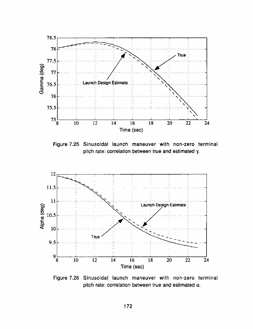
78.5

O)O

"10v

EE

(.9

78

77.5

77

76.5

76

75.5

758

! ! / True i

......._Lau_o.,oo_=,.o,........!.....:: ........,.......

:,,\i i i i i i i _.

10 12 14 16 18 20 22

Time (sec)

24

Figure 7.25 Sinusoidal launch maneuver with non-zero terminal

pitch rate: correlation between true and estimated 7.

12

11.5

11

O)

"O"" 10.5t,---c-!

< 10

9.5

9 i

8 10

_i I : Launch DesignEstimate :

i , ;12 14 1'6 1'8 2'0 22 24

Time (sec)

Figure 7.26 Sinusoidal launch maneuver with non-zero terminal

pitch rate: correlation between true and estimated oc.

172

7.8.4 Sinusoidal Launch Maneuver Parameter

Adjustment

The sinusoidal launch maneuver is a function of two parameters, Tkick,

and, f2. As shown in Figure 7.1, Tkick represents the length of the maneuver

and f2 is a value equal to half the maximum commanded pitch rate. During the

launch design process, the user specifies the desired 0 and o_ at the end of

Phase Two. The process of then choosing the correct combination of mkick and

D. to ensure a "smooth" transition to Phase Three is an iterative procedure. That

procedure involves minimizing the error between the estimated ct, as computed

by the launch design simulation, and the desired o_at the end of launch. The

other terminal launch state, 8, is a function of f_, Tkiek ' and 0initial. This is

demonstrated by integrating the equation of the sinusoidal launch profile, which

is:

0ol,cost t))[TKick

Integrating the left side of Equation (7.11) results in

t=TKicko dt = OFina 1 - Olnitia 1

=o

(7.12)

Similarly for the right side of Equation (7.11):

dt = _ TKick (7.13)

Combining Equations (7.12) and (7.13), and solving for f2 yields

173

= 0 Final - 0 Initial (7.14)TKick

Initially, the minimization algorithm selects a value of Tk_ k with which to

estimate the terminal launch states. _ is then calculated based on Equation

(7.14) and a simulated launch is performed. The results from the simulated

launch are then compared to the desired terminal launch states. If the

estimated terminal states and the desired states are not identical, then a new

value of Tkick is chosen using a golden search bisection. A new [2 is then re-

calculated and the launch simulation is re-run until the error in terminal states is

minimized. The complete procedure is shown in Figure 7.27. The values of

Tkick chosen by the launch design algorithm are always rounded to the nearest

0.1 sec to conform to the integration step time of both the simplified launch

simulation and the full 6 DOF simulation. In addition, the launch design

algorithm continually adjusts Tkick until the predicted error in alpha final is less

than 0.05 ° or the value of Tkick yielding the minimum error in alpha has been

located within 0.1 seconds.

7.8.5 Parameter Adjustment for the Sinusoidal

Launch Maneuver with a Non-zero

Terminal Pitch Rate

The second launch profile employing a non-zero terminal pitch rate is

illustrated in Figure 7.2, and is characterized by two different phases. During

the first half of the maneuver the vehicle is commanded to follow a sinusoidal

pitch rate command. When the commanded pitch rate has reached its

maximum value at t =Ttran s, the commanded pitch rate is held constant until the

end of the maneuver. Termination of the launch profile occurs at t = Tkick. A

non-zero terminal pitch rate means that one extra variable is necessary to

define the launch profile. This allows the user to match not only the desired

attitude and angle of attack at the beginning of Phase Three, but also the

attitude rate.

174

--_ ICalculate _ based"Y I on desired end of

I launch theta and[ Tkick

Initialize routine withcurrent state values

at the end of Phase One

Simulate launch using 2 DOFpitch plane model using specified

values of theta, P,,and Tkick.

_=_ISelect desired end Iof launch theta

Ic.oo.ea.a,oe6___Jse,e I - [ of launch alpha J

OLestimate d - (Xtrue < 0.05 °

._ Adjust the value of ]'kick using a golden I

I

ratio bisection to minimize the error in (x. I

End of launch maneuverdesign: return value of

Tkick and Q.

Figure 7.27 Sinusoidal launch maneuver design flow chart.

The process of determining the launch design parameters for the non-

zero terminal pitch rate maneuver again involves a minimization of ¢ with mkick

as the free variable. The end of launch states e, and e are further related to the

launch maneuver transition time, Ttran s. This is proven by first integrating the

launch profile.

175

t = TTraa sdt =

Jt=O Jt=O

o(1_oos t)),t t ,, TKi, k+ 2_ dt

• 't = TTrut

(7.15)

From Equation (7.15), the change in attitude over the length of the

maneuver can therefore be written as:

OFina I -Oinitia 1 = -f_ TTran s + 2k"2 TKick

or AO = -f_TTran s + 2_TKick (7.16)

Solving Equation (7.16)for Ttran s yields:

A0 - 21"2TKickTTran s - (7.1 7)

-f_

A necessary condition is that the right side of Equation (7.17) is always

positive. This restricts the value of Tkick chosen for the launch simulation by

the relationship:

TKic k _> A0 (7.18)2f_

The flow chart shown in Figure 7.27 for the sinusoidal launch maneuver,

is also applicable to the sinusoidal launch maneuver with a non-zero terminal

pitch rate. The only additional calculation performed by the sinusoidal launch

maneuver with a non-zero terminal pitch rate is the calculation of Ttran s.

176

Chapter Eight

SIMULATION RESULTS

8.1 Introduction

Two different sets of simulation runs with and without the effects of signal

quantization were made. The first set was made to evaluate the acceleration-

direction guidance, steering and control concept for ideal feedback variables.

The second set was made to evaluate the performance of the rate, angle of

attack, and dynamic pressure estimators. The runs in the first set, listed in Table

8.1, are based on the feedback of true angular rate, angle of attack, and

dynamic pressure. Plotted results of these runs are shown in Figures 8.1

through 8.11. The maximum Q and Qo_values for each of the runs are tabulated

in Table 8.2. The runs in the second set, listed in Table 8.3, were made using

different combinations of true and estimated angular rate, angle of attack, and

dynamic pressure. Plots showing the effectiveness of the estimators are

illustrated in Figures 8.12 through 8.25. The maximum values of Q and Qo_ for

each of these runs are shown in Table 8.4.

The results presented in this chapter are preliminary. The effects of

bending and fuel slosh are omitted. The engine nozzle actuators are assumed

to provide perfect instantaneous response to the nozzle command subject only

to the limitation that the change in nozzle deflection not exceed 1° from one

sampling instant to the next (this is equivalent to a nozzle rate limit of 10°/sec).

The tail-wags-dog effect is also omitted. The effects of varying the levels of IMU

quantization on the angular rate and angle of attack estimators are examined in

Chapters Four and Five.

For each run in Table 8.1, a separate trajectory design was first carried

out to optimize the predicted on-orbit mass of the vehicle and minimize the

change in pitch attitude at the transition to PEG. For the first four runs the

trajectory design was done for a variety of winds with the design Q(z limit set at

3000 Ibs deg/ft 2. For run number 5, the vehicle was oriented differently with the

177

core stage on top of the booster during flight. To take advantage of the

improved performance offered by this alternative orientation the design Qo_ limit

for this configuration was reduced to 2800 Ibs deg/ft 2. For each optimal

trajectory design the filtered acceleration-direction was stored as a function of

time so that it could be later employed in an actual flight employing the

acceleration-direction concept. The trajectory design simulations were run

using the Vandenberg #69 wind profile exclusively in either a tail or head wind

direction. The magnitude of the winds was determined by scaling the stored

wind profile by a fixed percentage.

To test the performance of the acceleration-direction concept each stored

acceleration-direction profile was employed in an actual in-flight simulation

employing a different wind profile. For each acceleration-direction flight

simulation the Vandenberg #70 wind profile was employed at different

magnitude levels in either a head or tail wind direction. In addition to having a

slightly different wind profile shape, the Vandenberg #70 profile has wind

magnitudes that are approximately twice those of the Vandenberg #69 profile.

By flying the acceleration-direction concept in a wind profile that was different

than the wind profile used during the trajectory design, the effectiveness of the

acceleration-direction concept in providing adequate load relief as well as

accurate trajectory following was tested.

For all of the runs listed in Table 8.1 an in-flight Qo¢ limit of 3350 Ibs

deg/ft 2 was employed during the acceleration-direction simulations. This Q_

limit was higher than the trajectory design Qo¢ limit of 3000 Ibs deg/ft 2 used for

the first four runs and also higher than the 2800 Ibs deg/ft 2 used for run number

5. The larger in-flight Qo: limit values are necessary so that when variations

from the pre-launch winds are encountered, there is enough latitude within the

Qa limit to adjust the trajectory.

As mentioned above, the performance of the angular rate, angle of

attack, and dynamic pressure estimators was tested by employing a second

category of runs. For each run listed in Tables 8.3 and 8.4 (runs 6-10) a

quantization level of 3 arcsec was assumed in the measurement of Ae and a

quantization level of 0.0128 ft/sec was assumed in the measurement of AV. For

the sake of comparison, each run was made using the worst-case flight

conditions listed under "run # 1" in Table 8.1. As shown in Table 8.4 all of the

acceleration-direction runs with estimators and signal quantization were made

178

with the Q(_ limit increased to 3500 Ibs deg/ft2. This higher limit was required to

accommodate the increased errors in the estimated Q(z resulting from

quantization. (This includes run #10 which represents the alternative vehicle

configuration in which the core stage rides on top of the booster stage.) The

trajectory design Q(z limit was set at 3000 Ibs deg/ft 2 for runs #6 through #9, and

2800 Ibs deg/ft 2 for run # 10.

Trajectory Design SimulationA pitch On-

Run @ PEG orbit Figure

# Wind Magnitude Wind Wind Magnitude Wind (deg) Mass #

Direction Profile # Direction Profile # (slugs)

1 Head 60% 69 Head 60% 70 4.04 12130 8.1-8.3

2 Head 40% 69 Head 40% 70 1.40 12147 8.4-8.5

3 Tail 60% 69 Tail 60% 70 -0.11 12191 8.6-8.7

4 Tail 40% 69 Tail 40% 70 -0.05 12182 8.8-8.9

8.10-5* Head 60% 69 Head 60% 70 1.31 12212

8.11

Table 8.1 Simulation results for acceleration-direction concept with

the true feedback variables.

179

Run # Maxlmum Q Maximum

Qcz limit

Trajectory

Design

Q(x limit

Simulation

1 849.5 3431 3000 3350

2 862.1 3404 3000 3350

3 768.8 3272 3000 3350

3169

3570

772.8

927.9

3000

2800

4

5*

Table 8.2

3350

3350

Maximum Q and Qo_ values for acceleration-direction

concept simulations with true feedback variables. (* Core

on top of booster.)

Run

#

6

7

8

9

10"

_T_e

Yes

(z

Yes

Yes

Yes

- Yes

Table 8.3

Feedback Variable ,_ Pitch On-orbit

Q @ PEG Mass Figure

O)True _ QTrue C} (deg) (slugs) #

Yes Yes 2.46 12136 8.12-8.13

Yes - Yes 5.06 12134 8.14-8.15

Yes Yes - 4.46 12118 8.16-8.17

Yes 4.57 12128 8.18-8.21

Yes 1.90 12210 8.22-8.25

Yes

Yes -

Simulation results for acceleration-direction concept using

estimated angle of attack, angular rate, and dynamic

pressure. (* Core on top of booster.)

180

Run # Maximum Q

MaximumO_

Qoclimit

TrajectoryDesign

Q(x limit

Simulation

6 837.2 3583 3000 3500

7 862.1 3603 3000 3500

8 855.8 3579 3000 3500

3592

3692

857.4

940.6

3O00

2800

9

10"

Table 8.4

3500

3500

Maximum Q and Qoc values for acceleration-direction

concept simulations using estimated feedback variables.

(* Core on top of booster.)

8.2 Discussion of Results

For the first run tabulated in Table 8.1 the vehicle was flown in a head

wind corresponding to 60% of the Vandenberg #70 profile. This head wind had

wind velocities which were greater than the 60% Vandenberg #69 wind profile

used during the trajectory design process. As shown in Figure 8.1, this

increased level of head winds caused the flight control system to switch to the

Qoc limiting mode to prevent the angle of attack of the vehicle from exceeding

the angle of attack limit, _lim_" As shown in Figure 8.2 this resulted in the vehicle

closely following the Qoc limit of 3350 Ibs deg/ft 2. By switching from

acceleration-direction steering to angle of attack feedback the flight control

system was able to provide quick load relief performance.

In Figure 8.3 it can be seen that the vehicle spent approximately one half

of Phase Three flying in the Qcx limit mode. The effect of this long period of Q_-

limiting load relief is to cause the attitude of the acceleration vector to be slightly

lower than the attitude for the corresponding nominal trajectory design case.

181

Despite this effect on the trajectory, only a 4.02 ° change in attitude was

commanded at the transition to PEG. As shown in Table 8.1, this also resulted

in a predicted on-orbit mass of 12130 slugs which is slightly lower than the

corresponding trajectory design prediction of 12136 slugs -- a decrease of only

6 slugs.

Run #2 was also a head wind case, but the magnitudes of winds

employed in both the trajectory design and the actual in-flight simulation were

only 40% of the full Vandenberg #69 and #70 wind profiles. In the presence of

lighter winds the performance of the vehicle improved. The predicted on-orbit

mass of 12147 slugs for the in-flight simulation was higher than that predicted

for run #1, and the change in commanded attitude at the transition to PEG was

only 1.40 °. This improvement in performance was at least in part due to the fact

that the vehicle spent a shorter time period in the Qo_ limit mode. This can be

seen by comparing Figure 8.5 and Figure 8.2. As shown in Figure 8.5 the

vehicle again closely follows the Q¢ limit of 3350 Ibs deg/ft 2 but its duration at

that limit is much shorter than that of Figure 8.2. Asa result the vehicle spends

a larger portion of time in the latter stages of Phase Three flying in the

acceleration-direction mode. The decrease in on-orbit mass from the trajectory

design to the subsequent flight is only 3 slugs. This smaller decrease in mass

can be attributed to the fact that the reduced-magnitude winds result in smaller

differences between prelaunch (design) winds and flight winds which in turn

result in less of a trajectory change being produced by wind produced Qa-

limiting.

For runs #3 and #4 the vehicle was subjected to tail winds of the same

magnitudes as in runs #1 and #2, respectively. As shown in Figures 8.6 and 8.7

the angle of attack of the vehicle in both tail wind runs remained below the

angle of attack limit at all times. As a result the vehicle did not enter the Qo_limit

mode at any time during Phase Three. This is illustrated in Figures 8.7 and 8.9

where it can be seen that the Qa of the vehicle remains below the Qo_ limit of

3350 Ibs deg/ft 2.

As shown in Table 8.1, the effects of the tail winds for both run #3 and run

#4 improved the in-flight predicted on-orbit mass performance of the vehicle

compared to the head wind in-flight simulations. In comparing run #3 (60% tail

wind) to run #1 (60% head wind) it can be seen that the on-orbit mass improved

by 61 slugs (from 12130 slugs to 12191 slugs). An improvement in on-orbit

182

mass can also be seen when comparing the trajectory design simulations of

runs #3 and #4 with their corresponding in-flight simulations. For run #3, the in-

flight simulation yielded an improvement of 10 slugs over the trajectory design

simulation, and for run #4, the improvement from trajectory design to in-flight

was 6 slugs. For both tail wind cases the change in commanded attitude at the

transition to PEG was no different than that seen in the corresponding trajectory

design simulations. As shown in Table 8.1, the change in pitch attitude at PEG

for both run #3 and run #4 was less than 0.2 °.

As previously mentioned run #5 was made with the alternative

configuration of the core stage riding on-top of the booster. For the sake of

comparison the trajectory design and in-flight simulations were run in the same

wind profiles as in run#1. As shown in Table 8.2, the trajectory design for this

alternative configuration was carried out with the slightly lower Qo_ limit of 2800

Ibs deg/ft 2. This decrease in the Qo_ limit provided the vehicle with some added

latitude in adjusting the trajectory in the presence of off-nominal winds. In

comparing Figure 8.10 and Figure 8.1 it can be seen that with the alternative

configuration the vehicle spent less time flying in the Qe_-Iimiting mode.

Consequently, the load relief was applied for a shorter time in run #5 compared

to run #1 and this helped reduce the trajectory deviations throughout Phase

Three. This improvement in design-trajectory following is evidenced by the

lower commanded attitude change at PEG (1.31 ° for run #5 vs. 4.04 ° for run #1).

In addition to this performance improvement there was also a significant

improvement in the predicted on-orbit mass of the vehicle. As shown in Table

8.1 the predicted on-orbit mass of 12212 slugs for run #5 was 82 slugs more

than that predicted for run #1. Such an improvement is significant, especially

since the predicted on-orbit mass for both tail wind simulations was also less

than that predicted for the alternative configuration.

With the utilization of perfect feedback the performance of the

acceleration-direction steering concept with Qe_-Iimiting load relief provides

excellent trajectory shaping capability as well as accurate and fast load relief

performance in the presence of off-nominal winds. For the first four trials in

Table 8.1 the difference between the trajectory design Qo_limit and the selected

in-flight Qo_ limit was only 350 Ibs deg/ft 2. For run #5 a larger difference of 550

Ibs deg/ft 2 was available because of the improved trajectory shaping

capabilities offered by this orientation. Both margins, while quite small,

183

provided enough latitude to allow the flight controller to maintain the desired

trajectory in the presence of small wind disturbances.

To study the effects that estimated feedback quantities would have on the

performance of the acceleration-direction steedng concept, two additional runs

were made. These runs, which are tabulated in Table 8.5, were made with the

same flight conditions as run #1. The first line of the table is a duplication of the

results presented for run #1, which was made using true values of the feedback

variables. The first of the two additional runs was made with estimated angular

rate and angle of attack feedback but without any quantization in the signals

processed by the estimators. For the final run quantization was added to the

signals processed by the estimators.

Comparing the first of the additional runs with the run using true feedback

variables it can be seen that the utilization of estimated feedback variables

degraded the performance. The predicted on-orbit mass of the vehicle

decreased by 15 slugs (from 12130 slugs to 12115 slugs) and the attitude

change at PEG increased by 1.89 ° (from 4.04 ° to 5.93°). In addition, although

the maximum value of Qa decreased, it will be shown that this reduction is due

to errors associated with estimating the angle of attack.

For the second of the additional runs quantization levels of 3 arcsec and

0.0128 ft/sec respectively were assumed in the measurements of A8 and _V.

As shown in the last row of Table 8.5 this added effect further degraded the

performance of the system. Compared to the results tabulated for true variable

feedback, the predicted on-orbit mass of the vehicle decreased by 27 slugs

(from 12130 slugs to 12103 slugs) and the attitude change at PEG increased by

3.05 ° (from 4.04 ° to 7.09°). In addition, the added effect of quantization

increased the maximum value of Qa to 3513 Ibs deg/ft 2, or 163 Ibs deg/ft 2 above

the in-flight Qa limit. This loss in performance is partly due to the combined

effects of lags associated with estimating the feedback quantities, and the

quantization introduced into the measurements of A0 and &V. As a result of this

loss in performance it was decided to increase the in-flight Qa limit to 3500 Ibs

deg/ft 2 for the runs (6-10) listed in Tables 8.3 and 8.4.

For run #6, the estimated angular rate (see Chapter 4), the true angle of

attack and the true dynamic pressure were employed. As shown in Figure 8.12,

184

Flight Condition

Feedback

or., co

Quantization

No

pitch

@ PEG

(deg)

4.04

On-orbit

Mass

(slugs)

Maximum

Oo_

(Ibs deg/ft 2)

12130 3431

_,_ No 5.93 12115 3407

Yes 7.09 12103 3513

Effects of estimators and quantization on performance of

run #1.

,CO

Table 8.5

the larger head wind magnitudes encountered in-flight forced the vehicle to

enter the Qoc-limiting mode to prevent the angle of attack from exceeding the

angle of attack limit, _limit. AS shown in Figure 8.13 this resulted in the vehicle

closely following the larger in-flight Qcx limit of 3500 Ibs deg/ft 2. The effect of

increasing the Qoc limit upon the predicted on-orbit mass can be seen by

comparing run #1 and run #6. Despite feeding back estimated angular rate

(which in theory should degrade the performance), the on-orbit mass of the

vehicle improved by 6 slugs -- from 12130 slugs to 12136 slugs. Increasing the

Qo_ limit also improved the trajectory-following capability of run #6 which is

demonstrated by the lower attitude change at PEG.

For run #7, the estimated angle of attack (see Chapter 5), the true

angular rate and the true dynamic pressure were employed. As shown in Table

8.3 the use of estimated angle of attack alone had a larger impact upon the

performance of the system than the estimated angular rate alone (run #6).

Although the loss in predicted on-orbit mass was only 2 slugs the attitude

change at the transition to PEG increased to 5.06 °. As illustrated in Figure 8.14

the true angle of attack of the vehicle tended to lead the angle of attack limit

throughout most of Phase Three. As a result, the Qo_of the vehicle tended to be

below the in-flight Qo_limit of 3500 Ibs deg/ft 2. This effect is illustrated in Figure

8.15.

The combined effect of estimated angular rate and angle of attack

feedback on system performance are shown in Figures 8.16 and 8.17 (run #8).

185

It can be seen that the angle of attack and Qo¢of the vehicle throughout Phase

Three were very similar to those illustrated in Figures 8.14 and 8.15 for run #7.

As shown in Table 8.3 the predicted on-orbit mass for run #8 was 12118 slugs.

This prediction of on-orbit mass was 16 slugs less than that predicted for run #7

and 18 slugs less than that predicted for run #6. This loss in performance is

expected since run #8 employs two estimated feedback variables while run #6

and run #7 employ only one.

For run #9 The angle of attack, the angular rate, and the dynamic

pressure estimators were all employed in the in-flight simulation. As shown in

Figures 8.18 and 8.19 the performance of the system was very similar to the

results presented for run #8. As shown in Table 8.3, the change in commanded

attitude at the transition to PEG was 0.11 ° greater than that reported for run #8.

In addition, the predicted on-orbit mass was 12128 slugs, which is an increase

of 10 slugs over the previous run.

For run #10 the alternative orientation of the core riding on top of the

booster was employed. For the sake of comparison the in-flight simulation was

made using estimated angle of attack, estimated angular rate, and estimated

dynamic pressure, as in run #9. As shown in Table 8.4, the trajectory design for

this alternative configuration was carried out with a slightly lower Qo_ limit of

2800 Ibs/deg ft2. In comparing Figure 8.21 and 8.18 it can be seen that with the

alternative configuration the vehicle spent less time flying in the Qo_-Iimiting

mode. Consequently, the vehicle spent more time in the acceleration-direction

mode and this improved the trajectory following throughout Phase Three. This

improvement is evidenced by the lower commanded attitude change at PEG

(1.90°). In addition, there was also a significant increase in the predicted on-

orbit mass. As shown in Table 8.3 the predicted on-orbit mass was 12210

slugs, or 82 slugs higher than that predicted for run #9. In comparing run #5 to

run #10, it can be seen that the use of estimated feedback quantities only

slightly degraded the performance in the case of the core riding on top of the

booster. For both the commanded attitude change at PEG as well as the

predicted on-orbit mass the difference between the two runs was minimal.

The effect of feeding back both the estimated angular rate and the

estimated angle of attack upon the commanded nozzle deflection is illustrated

in Figure 8.20. As shown the nozzle command fluctuates more during the initial

portions of the Qo_ limit mode. In addition, these fluctuations are less during

186

periods where the vehicle is in the acceleration-direction mode and the angle of

attack is no longer being employed as a feedback variable. These fluctuations

are due in part to the effects of quantization as well as the transient behavior of

the angle of attack and angular rate estimators. The amplitude of these nozzle

command variations illustrated in Figure 8.20 do not exceed the rate limit of the

nozzle actuators at any time.

2O

15

O"10v

¢_ 10t-O.

,,(

5

_ _ O_Limit

a"

i i i (_ i /

• • i 1S

............. i .............. _. ................................... 7" ......

_) I I IO0 4 60 80 100

Time (sec)

.J120

Figure 8.1 Angle of attack and angle of attack limit with perfect

feedback in 60% Vandenburg #70 head wind.

187

3500

3000

1500

1000 i |

20 40 60 80 100 120

Time (sec)

Figure 8.2 Qo_ and Q(z limit with perfect feedback in 60% Vandenburg

#70 head wind.

08O

Time (sec)

Figure 8.3 Commanded nozzle deflection for Angle of attack and angle

of attack limit with perfect feedback in 60% Vandenburg

#70 head wind.

188

25

2O

c_ 15Q)"IE}v

t-O. 10<

__ (ZLimit_ : ................................................ //

k (

..... _, ............................................................. i f ....

" i.............. i ............. i .......... "" ........

t i i I

O0 40 60 80 lO0 120

Time (see)


feedback in 40% Vandenburg #70 head wind.

3500

¢xl41

"k

"IDtl)t'_

0

,ooo-....._ ; _.... ....._..............................t33,o2500

2000

1500

1000

50020 40 60 8'0 1()0 120

Time (sec)

Figure 8.5 Q oc and Qoc limit with perfect

Vandenburg #70 head wind.

feedback in a 40%

189

25I

(t

20 .... x................................................................... , -

_X / (XLimit t t

15 ....... _(_,'< ................................................. _i ......(X

_ _ r t........... %, ................................................ f ............

%%1 . . .f

t_e-

10<

5

| I 810 IO0 40 60 l O0 120

Time (sec)

Figure 8.6 Angle of attack and angle of attack limit with perfect feedback in

60% Vandenburg #70 tail wind.

3500 , : :

3000

,_-_ 2500

• 2000

1500

1000

5%0 4'0 60 80 1130 120

Time (sec)

Figure 8.7 Q_ and Qe_ limit with perfect feedback in a 40% Vandenburg #70

tail wind.

190

25

2O

o_ 15

v

¢-o_ 10!<

5

. . .'t. "¢

Or.Limit //

..... _ ...... !................................................... ,;_ ....

\\_,,Z" " " s _

0 i i i I

20 40 60 80 100 120

Time (see)


feedback in 40% Vandenburg #70 tail wind.

3500

300O

A

2500

• 2000

.ID

_ 15000

1000

5 40 60 8'0 100 120

Time (sac)

Figure 8.9 Q a and Qo_ limit with perfect feedback in a 40%

Vandenburg #70 tail wind.

191

2O

15

v

10t.-

5

02O

L/

/

Or,Limit t/

• ' i . z,

Figure 8.10

' 6() ' '40 80 100 120

Time (sec)

Angle of attack and angle of attack limit with perfect

feedback in a 40% Vandenburg #70 tail wind with the core

stage riding on top of the booster stage.

3500

.............. i .............. i............... i .............. ..........

.it

.It

OI

itim

v

3000

2500

2000

1500

1000

5002O

Figure 8.11

* I I I

40 60 80 lO0 120

Time (see)

Q o_ and Qo_ limit with perfect feedback in a 60%

Vandenburg #70 head wind with the core stage riding on

top of the booster stage.

192

25

2O

o) 15"IDv

¢- 10

_' _ GLimit

f

................. ......................".. ,.,;......

i I I

SO 40 60 80 100 120

Time (sec)

Figure 8.12 Angle of attack and angle of attack limit with estimated

feedback of angular rate in a 60% Vandenburg #70 head

wind.

4OOO

3500

2000

1500

lO00

50020 40 lO0

ea 300041

i:_ 2500Q)

"0o')

I

60 80 120

Time (see)

Figure 8.13 Qo_ and Q(z limit with estimated angular rate feedback in a

60% Vandenburg #70 head wind.

193

25

2O

"-'15(p"Ov

_- I0Q.

<

I | | I

O0 40 60 80 1O0 120

Time (sec)


feedback of angle of attack in a 60% Vandenburg #70 head

wind.

4OOO

3,° .... ; !35o,

"_ 2500 -

1500 ........................................................................

%; , ,1 4}? 60 80 100 120Time (sec)

Figure 8.15 Qo_ and Qo_ limit with estimated angle of attack feedback in

a 60% Vandenburg #70 head wind.

194 C -

25

2O

c_ 15

v

t-O. 10<

-- tl ..............................................

_ _ Or'Limit

....... _'_,,:.............. i............. i......... _;.'" ......

i I I I

20 40 60 80 100 120

Time (sec)


feedback of angle of attack and angular rate in a 60%


4O0O

oJ

"10

v

3500

3000 0

2500

_ 2ooo

1500

000i L_ i I1 20 40 ou 80 100 120

Time (sec)

Figure 8.17 Qo_ and Qe_ limit with estimated angle of attack and angular

rate feedback in a 60% Vandenburg #70 head wind.

195

25

2O

15"O

t_t--

o_ 10<

5

02O

x _ Or,Limi t

..... 1 .................................................................

• \........... '%, ..................................................... J .......

• , , _ •

Figure 8.18

I I i I

40 60 80 100 120

Time (sec)

Angle of attack and angle of attack limit with estimated

feedback of angle of attack, angular rate, and Q in a 60%


4000

3500

2500

:ooo1500

100020

Figure 8.19

I i I i

40 60 80 100 120

Time (sec)

Q(z and Q_ limit with estimated angle of attack, angular

rate, and Q feedback in a 60% Vandenburg #70 head

wind.

196

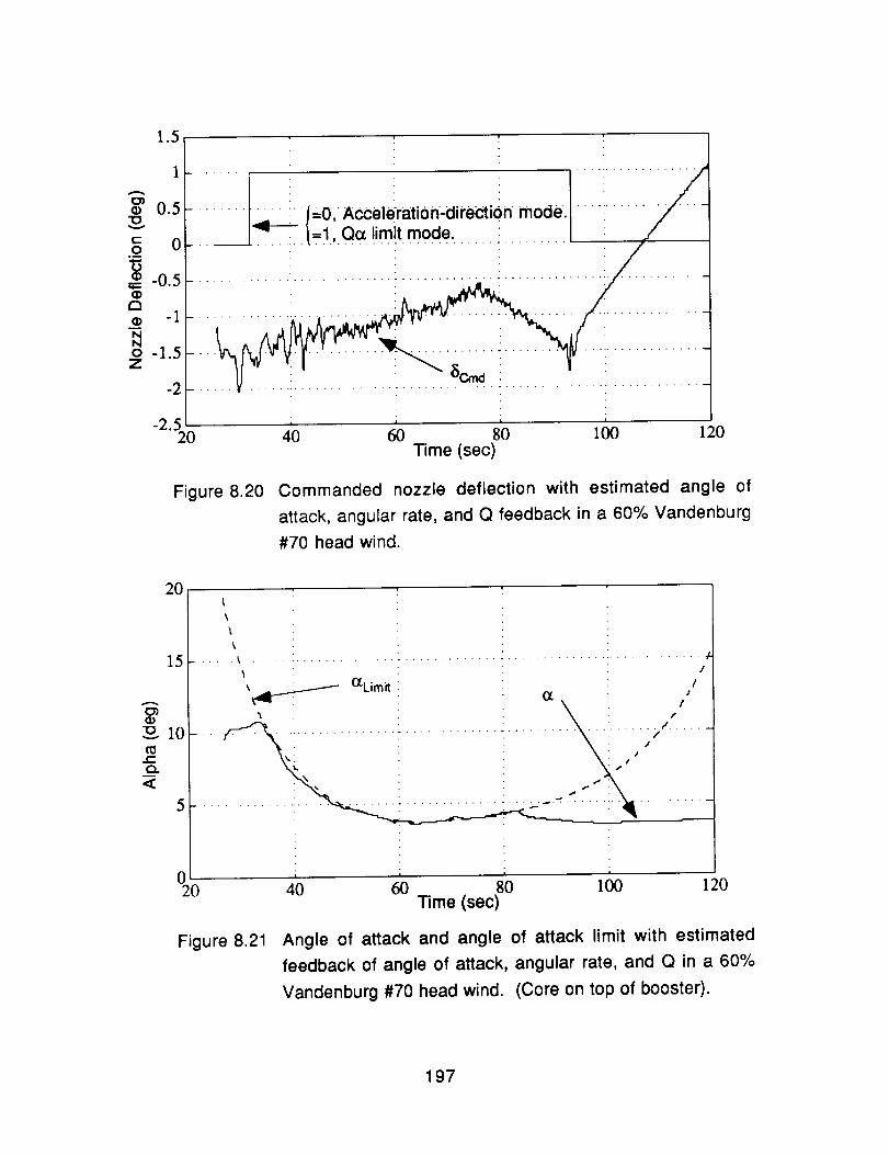
1"51 : :

1- : ,=u _cce, eauono, recuonmode, i i__ 0.5 ....... ..... -,-,,.,.., _-_,-r_-..,-..--...-__._.-._..:--: . .... .......

'-" 0.o

=_-0.5

a-I

NNo -1.5 -z ii

-2

25 ....- I i I I

20 40 60 80 100 120(sec)

Figure 8.20 Commanded nozzle deflection with estimated angle of

attack, angular rate, and Q feedback in a 60% Vandenburg

#70 head wind.

2O

15

A

"_ 10v

t-

<

5

L

..... _ ....... i......................................................... S

I I I I

O0 40 60 80 100 120

Time (sec)


feedback of angle of attack, angular rate, and Q in a 60%

Vandenburg #70 head wind. (Core on top of booster).

197

4OOO

3500

3000,Itit

2500

x_ 2000

_ 1500

1000

i i i i

50020 40 60 80 100 120

Time (see)

Figure 8.22 Qo_ and Qo¢ limit with estimated angle of attack, angular

rate, and Q feedback in a 60% Vandenburg #70 head

wind. (Core on top of booster).

• {=0, Acceleration-direction mode."_ -1 =1; Qo_ limit mode. .............. i..............(D

cO

_5 -3m

121 -4

NN -5Oz

i _cma ! ! i

iii i i i-6

-720 ....40 60 80 100 120

Time (sec)

Figure 8.23 Commanded nozzle deflection with estimated angle of

attack, angular rate, and Q feedback in a 60% Vandenburg

#70 head wind. (Core on top of booster)

198

Chapter Nine

CONCLUSIONS AND RECOMMENDATIONS

9.1 Conclusions

The primary purpose of this thesis was to develop and evaluate an

integrated concept of guidance, steering, control, load relief and estimation for

application to the asymmetrical configuration of the Advanced Launch Vehicle

(ALS). This concept is preliminary in that it was developed for an early ALS

design for which comprehensive aerodynamic data, bending and slosh data,

engine nozzle actuator data and IMU characteristics were not available. As a

result, certain details had to be omitted from the system models and from the

designs of the control and estimator systems. It is also preliminary in that much

remains to be done in exploring predictive-adaptive concepts in guidance and

control that might give the ALS greater flexibility and better performance in

dealing with the effects of last-minute changes in payload, vehicle configuration,

mission objectives and winds as well as in-flight changes in the wind

environment. Nevertheless, there are a number of new component concepts

and features embodied in this integrated concept that could provide a

considerable advancement over present methods, with or without predictive-

adaptive features.

The integrated concept that has been explored in this thesis centers on

the use of acceleration-direction guidance and control in combination with an

override control mode that limits the product of the dynamic pressure Q and the

angle of attack o_. This guidance and control approach has been studied for the

case of an acceleration direction command that is stored as a function of time

based on trajectory design computations that are carried out just prior to launch.

These prelaunch design computations shape the trajectory for winds that are

measured prior to launch with a specified Qo_ limit that is less than the limit

employed in flight. The difference between in-flight and prelaunch limits on Qe_

199

provides some leeway to adjust the in-flight trajectory to compensate for the

effects of changes in the winds from their prelaunch values.

As previously mentioned, the acceleration-direction guidance and control

approach and the associated trajectory design program build upon concepts

that were investigated earlier by Bushnell and Corvin, respectively. The

acceleration-direction guidance and control with the Qo_-Iimit override was

studied by Bushnell for the case of a symmetrical solid-propellant boost vehicle

whose ideal post-launch endoatmospheric trajectory was a zero-(z trajectory.

The employment of this approach in the case of a liquid-propellant

asymmetrical ALS with large angle of attack values and different vehicle

properties requires some modifications. The trajectory design program

developed by Corvin was for a guidance/steering system based on the flight

path angle and a control system based on the angle of attack. Corvin's program

generated a commanded flight path angle which was stored for in-flight use.

The ALS version of Corvin's program generates a commanded acceleration

direction for in-flight employment. In addition to these and other revisions in the

design program and the basic guidance and control approach, the ALS system

examined in this thesis includes new concepts in estimation of the angular rate,

angular acceleration, angle of attack and dynamic pressure.

The innovations which have been considered in this thesis for the ALS

application are:

(1) Alternative pitch rate profile for the launch maneuver which has a

constant pitch rate in the latter half of the maneuver.

(2) Utilization of the trajectory design simulation to compute an

acceleration-direction command for Phase Three by passing the simulation-

determined acceleration-direction through the same low-pass filter that is

employed in the in-flight acceleration direction estimator: This command is

stored for in-flight use.

(3) Employment of a different set of compensation gains for each of the

two control modes of Phase Three.

(4) Reinitialization of the forward-path control integral when switching

control modes in Phase Three so as to prevent the gain changes from

producing a step change in the engine nozzle command.

200

(5) Utilization of a first order complementary filter estimator to provide the

rate feedback, employing an estimated acceleration input that relies on a

feedback loop to estimate the angular acceleration produced by the

aerodynamic axial force in combination with the offset of the center of pressure

normal to the longitudinal axis.

(6) Employment of a second order complementary filter estimator to

provide the angle of attack feedback, taking advantage of the properties of the

second order estimator to minimize low-frequency errors produced by

neglecting the effects of the slowly varying flight path angle.

(7) Use of the estimated angle of attack in combination with the estimated

earth-relative velocity to estimate the dynamic pressure, approximating the

effects of winds by assuming they are horizontal.

Other elements of the flight and ground software system that was tested

in combination with the above features were based on the previous studies of a

Shuttle 2 SSTO system by Corvin which shaped the design trajectory for Phase

Three in terms of (_ and q_ profiles and which employed the predictive-

adaptive Powered Explicit Guidance in Phase Four. The simulation results,

which were based on a rigid -body vehicle model with ideal actuators and other

approximations, indicate reasonable overall performance with and without the

effects of quantization in the attitude and velocity signals.

9.2 Recommendations

The basic approach of acceleration-direction guidance and control with a

Qo_ override control mode, and the various features developed to implement

and accompany this approach, provide a good starting point for studies of

predictive-adaptive techniques for Phase Three in combination with

improvements of the methods employed in this thesis for the other flight

phases. More specifically, the following studies are recommended for future

consideration:

(1) Improve and automate the program for trajectory design (including the

possibilities of last-minute changes in the payload or the mission objectives).

201

(2) Effectively eliminate the adverse effects of errors in aerodynamicmodeling, dynamic pressure estimation and Mach number estimation on the

limiting of the angle of attack by defining the trajectory limit in terms of thenormal aerodynamic force rather than the Qo_product. (This procedure should

result in a more accurate limiting of the normal aerodynamic force than is

possible for the Qo_product.)

(3) Consider the possibility of including a variable roll attitude in the

trajectory design computations and also the possibility of changing the rollattitude in flight in a predetermined or adaptive fashion.

(4) Develop a predictive-adaptive guidance that adjusts an added rate

bias in the acceleration-direction command in the same way as Corvin has

adjusted a rate bias in a flight path angle command.1

(5) Compare the performance of the predictive-adaptive methods applied

to the acceleration-direction guidance-and-control approach and the Corvin

approach of guidance-steering based on the flight path angle in combination

with an inner angle of attack control loop.

(6) Investigate other more complex predictive-adaptive techniques as

applied to the more appropriate form of guidance and control.

(7) Utilize an updated simulation model of the ALS vehicle, including

more comprehensive aerodynamic data, nozzle actuator dynamics, tail-wags-

dog effects, bending modes, and ultimately including propellant slosh modes

and possibly the detailed engine nozzle command logic.

(8) Study the problem of bending mode compensation, possibly

considering adaptive techniques to deal with bending effects in the various

estimators.

1 Corvin, op cit.

202

Appendix A

Derivation of Equations of Motion

The angular momentum of a rigid body with respect to a fixed reference

frame, i, in inertial space can be written as:

H i =fr × V dm = f r x 1:i dm (A.1)

where

r = a position vector from q to a differential element dm.

_:i d i= r = the derivative of r taken relative to the inertialdt

frame i.

The derivative of r relative to the inertial frame i can be expressed as the

derivative relative to an arbitrary frame f by the relationship

or simply

dir =dfr + 0) fi X r

d t d t (A.2)

I:i= l:f+o) xr (A.3)

Substituting (A.3)into (A.1) yields:

Hi =fro r x rfdmr × (_o× r)dm

(A.4)

2O3

If we then require that frame f be fixed with respect to the rigid body, and

the origin of f coincide with the mass center of the body, then rt = 0 and

equation (A.4) reduces to:

r × × r)dm(A.5)

By introducing a set of body fixed orthogonal unit vectors (u], u 2, u 3) to

establish the orientation of frame f at the mass center, co and r can be

expressed as

r = rlu 1 + r2u 2 + r3u 3

o) - O)lU 1 + o)2u 2 + o)3u 3

(A.6)

(A.7)

Substituting these expressions into equation (A.5)

2)H = rE + r 3 o)] dm -

+[-f r2rl o31 dm+

+I-fr3rl (ol dm-

rlr 2 0) 2 dm - f rlr 3 0) 3 dm] U l

(rE + r_)o_ 2 dm-I r2r3 (03 dm

r3r2 o) 2 dm+I(r2 +r22)(03 dm

u2

u3

(A.8)

Or in matrix form

H

H1

H2 =

H3

111 I12 113

I21 I22 123

13 ] I32 I33 (A.9)

204

Where the diagonal terms I11, I22, I33 are called the principal moments

of inertia, and the off-diagonal terms are called the products of inertia.

It is assumed that for the ALS vehicle the body pitch, yaw and roll axes

(u], u2, u3) form a principal axes vector basis. Therefore, all of the off-

diagonal terms in Equation (A.9) are equal to zero. Equation (A.9) can then be

reduced to

H b = 111(01111 + I220)2u 2 + 133_3u 3 (A.IO)

The rate of change of the angular momentum relative to an inertially fixed

frame is equal to the vector sum, M, of all external torques on the system:

.iM = H (A.11)

.iIt is convenient to express H

fixed system b

in term of the derivative relative to the body

M H i H b= = +_xH (A.12)

Substituting (A.10)into (A.12) yields

n = (I1 1_1U 1 -4- I22tJ)2U 2 + I33(b3u 3)

+ (0)1U 1 + 02U 2 + 0)3U3)

× (II10)1U 1 + I220)2U 2 + I330)3U 3) (A.13)

M =[I1 10)1 - 0)20)3{I22 - I33)] Ul

+[I2 2Cb2 -0)30)1 (I33 - I1 1)] u2

+[I33_a - 0)10)2 (I11 I22)]113 (A.14)

205

Equivalently, the vector M in body coordinates is given by

Ill _1- C02 _3(I22 - I33)

I22 d)2- O)3 01 (I33 - I1 1)

133 &a- _1 O)2 (I 11 - I2 2) (A.15)

The expressions for the three components of M in (A.15) represent

Euler's Equation's of Motion.

206

Appendix B

Determination of Aero-Coefficients

Figure B.1 is a three dimensional sketch of a procedure for determining

the coefficient of normal force, Cn, given a Mach number and angle of attack.

The aero-data for the ALS was provided in a matrix format where each row of

data corresponds to a constant Mach number, and each column corresponds to

a constant angle of attack. The curves shown in Figure B.1 represent curve fits

of two adjacent rows from the aero data matrix. A total of fourteen such curves

comprise the matrix. Each curve is calculated by splicing together several third

order curves. Each third order curve spans two adjacent discrete Mach points

and its slope is continous from point to point. The "Low Mach" and "High Mach"

curves were found by determining which adjacent rows of the matrix bound the

current Mach number of the vehicle. The procedure for computing Cn from a

given Mach number and angle of attack is outlined in Table B.I. The same

procedure is used for determining the coefficient of axial force, Ca.

On

On

Out

Discrete Mach

Points

Third Order Spline

Segment

Low Mach

Curve

Figure B.1

_True

High MachCurve

Determination of Cn by Linear Interpolation.

Mach

Number

207

1)

2)

3)

Select the two 3dorder Cn vs o_curves that correspond to the

consecutive Mach numbers (MaChLo. and MaChHigh) that boundthe given Mach number, MaChTrue. These curves are designatedas the Low Mach and High Mach curves.

For the given value of angle of attack, Or.True,compute the valueof Cn on both the Low Mach and High Mach curves. - Points(_) and(_in Figure C.1.

Linearly interpolate in Mach number between points (_)and(_) to determine the value of Cn for Machmrue. - Point (_ inFigure C.1. This value is the desired value of Cn as a functionof GTrue and MaChTrue

Table B.1 Procedure for Determining On.

208

Appendix C

Determination of Mass Properties

In order to simulate the ALS vehicle, a simple model was constructed to

approximate the time varying mass, center of gravity location, and pitch moment

of inertia. The distribution of the total dry weight for each stage among all the

components was based on the percentage of volume that each component

occupied. In addition, because only the total height and width of each stage

was provided, all other dimensions such as the thickness of each fuel tank was

estimated. The data was provided by the General Dynamics Corportation,

Space Systems Division.

J8'

1

Booster Stage

0.15

46'

",_-- 0.15'

J L_..t__

15'

-T-

89'

I

I

I

/

I

/

I

/

I

/

I

I

/

tftf

IIIfIItI

/ f

l

30'

Figure C.1 Booster

Component

1 - Engine Module

2 - Hydrogen Tank

3 - Inter-Tank Adapter4 - Oxygen Tank5 - Nose Cone

Mass

(Slugs)

1688

2597117

1342

37

TOTAL 5781

Stage Component Masses and Dimensions.

2O9

Core Stage

Figure C.2

59'

I

/

_ 0.15'

Component

1 - Engine Module2 - Hydrogen Tank3 - Inter-Tank Adapter4 - Oxygen Tank5 - Payload Container6 - Payload7 - Nose Cone

Mass

(Slugs)

7232782

125115610104973

155

TOTAL 10924

Core Stage Component Masses and Dimensions.

210

Propulsion Module

Propulsion Module Booster Core

Mass of Engines 209.6 209.6

Number of Engines 7 3

Total Engine Mass 1467.3 628.8

Common Structure

@ 15% Total Mass 220.1 94.3

TOTAL MASS (Slugs) 1687.4 723.1

Table C.1 Core and Booster Propulsion Masses.

211

Appendix D

Vehicle Rigid Body Equations of Motion

The scope of this thesis is limited to the evaluation and study of flight

software concepts in the pitch plane. With this assumption, the trajectory pitch

plane motion of the vehicle can be defined by three differential equations. The

free body diagram of the vehicle in the pitch plane is shown in Figure D1. The

acceleration of the center of mass can be expressed in the earth relative

velocity direction frame (uvx, uvY, uvz) by the relationship:

[VV'E] relative to the local = lYrE]relative to the + (tO x VE)geographic framc velocity frame (D.1)

where co is the angular velocity of the velocity reference frame with

respect to the local geographic frame. Since the velocity is along the x axis of

the velocity direction vector,

['_/E] relative to the = WE UVX

velocity frame (D.2)

The rotation rate of the velocity coordinate system is the flight path angle

rate so that

co x V E = "yUVY x V UVX = -V_,UVZ (D.3)

Substituting Equations (D.2) and (D.3)into Equation (D.1),

VE = VEUVX - V_,UVZ (D.4)

212

V w

M E

T/

+z

Figure D.1 Vehicle Free Body Diagram.

Earth relative Horizontal

The corresponding equation of motion is given by

M V E = _, IF] Velocity frame (D.5)

Summing the forces in the uvx, and uvz directions yields the first two

equations of motion.

213

F,_ = -M_V = T b sin (_- (z)+ T c sin (8- (z) + Mg cos (7)

- SQC n cos (a)+ SQCa sin (a) (D.6)

E F_x = MV = T b cos (6- o_)+ T c cos (6- (z)- Mg sin (y)

- SQC a cos (a)- SQC n sin (or)

(D.7)

Summing the torque about the UVy axis yields the third equation of

motion,

Z TuvY = Iyy0 = T b sin (6)xcs + T c sin (6) xcs- Tb cos (6)(D + zcg)

- T c COS (6)Zcg + SQC n (lcp x - Xcg )+ SQC a (-lcp z + Zcg ) (D.8)

where

lyy = The inertia about the pitch axis.

M = The mass of the vehicle

SQCa = (Fa) = the axial component of the aerodynamic force.

SQC n = (Fn) = the normal component of the aerodynamic force.

g = gravity

°.

Solving Equation (D.8) for e yields:

*°

0=(T b + To)sin (6)xc8 _ Tbcos (6)(D + Ze$)

Iyy Iyy

+SQCn{lcpx - Xc8) +SQCa(-lcpz + Zc,g)

lyy Iyy

Tccos (6)zc$

Iyy

(D.9)

214

Solving Equation (D.6) for 4/yields

_,= (Tb+Tc) sin (8- at)- SQCncos (o0+ SQCasin to 0 + Mg cos (O- o_)-MV (D.10)

Since 7 = 0 - 6., Equation (D.10) can be solved for 6. to give

6. = f) + (Tb+T_) sin (8- or)- SQCnCOS to0+ SQCasin (a)+ Mg cos (0- o_)MV (D.11)

Linearized Equations of Motion

Equation (D.9) can be linearized by the following approximation:

D0,,,,_=_ae_,_+_,_o_

aa (D.12)

where A denotes a perturbation of the state variable from its nominal

value along the trajectory. The derivatives on the right side of Equation (D.12)

can be approximated by:

_90 _ (Tb+Tc)Xc,g cos (CSss)+ T b (D+zc8) sin (_Sss)+ T c zc8

25 lyy (D.13)

°,

D0t3o_

(_ _(1,_,-x_)Cn)SQ_a,, (bpx-xcs)+ a,,Iyy

215

+so tlcpz•zc,l+lc z-c,I

Iyy (D.14)

The derivatives of (lcpx- Xcg)and (-lcpz + Zeg)with respect to (z are

assumed to be negligible for this thesis study. Substituting Equations (D.13)

and (D.14) into Equation (D.12) yields the following rigid body state equation

A0""- (Tb+Tc) Xc$ cos (Sss) + T b (D+zc_) sin (8,,)+ T c zc$ sin (Sss) A8

Iyy

+SQCno(%x- x_,)+SQC=(%_+zo,)_Iyy (D.15)

Equation (D.11) can be linearized by the following approximation.

_O _8 _O(D.16)

The derivatives on the right side of Equation (D.16) can be expressed as:

O& - -g sin (Tss)/)0 V

(D.17)

o_ _ (Tb+T¢)cos (Sss-O_ss )

38 MV(D.18)

(D.19)

216

a&m

o_et

+

-(Tb+Tc)cos(_..-o..)-SQ(_co,,o._.,-C_sin(°..,)MV

(_ )+ v }SQ sin (O_ss) + C a cos (Ot,s) g sln(ys,)

MV (D.20)

Substituting Equations (D.17)through (D.20)into Equation (D.16) yields

the following state equation

A& = --£g sin (Yss) AO + A0 + (Tb+Tc)cos (Sss-(x,,) A5 +V MV

gsin (Yss), (To+T¢)cos (Sss- (Zss)

V MV

SQ ( C.a sin (ass) + C a cos (ass))] Aa

MV

SQ(Cna cos (ass)- C n sin (ass)) +

MV

(D.21)

Rigid Body Poles

Given the linearized state equations in (D.15) and (D.21) define

C1- 1 {_(Tb+Tc ) cos (Sss-ass)- SQ(Cn(_ cos (etss) - C n sin (ass))+MV

SQ( Caa sin (o%s)+ Ca cos (o%s) )} (D.22)

C2 = g sin (Yss)V (D.23)

C3 = (Tb+T¢)cos (Sss- otss)MV (D.24)

217

C4-SQCad-lcp z + Zcl_)

Iyy (D.25)

C5 - (Tb + Tc) xc6 cos (_,s)+ T b (D+zc6} sin (8,,)+ T c Zc_ sin (fi,,)

lyy Iyy lyy (D.26)

Equations (D.15) and (D.21) can then be expressed as

A& = -C2 AO + AO + C3 A5 + (C2 + C1) Act (D.27)

A0 = C5 A5 + C4 Ao_ (D.28)

Typical values for C1, C2, C3, C4, and C5 at 8, 60, and 120 seconds from

ignition are shown in Table 1.1. C5, which is inversely proportional to the inertia

of the vehicle, increases during flight. The values of C1, C2, and C3 decrease

as the vehicle velocity increases. In Laplace notation Equations (D.27) and

(D.28) can be expressed as

(s-(CI+C2))Aot= (s- C2)AO +C3A5 (D.29)

s2Ae = C5 A5 + C4 Aot (D.30)

By solving for A(x in Equation (D.29) and substituting the result into

Equation (D.30), the rigid body transfer function relating the commanded nozzle

deflection to the resulting vehicle attitude can be expressed as

o(s,A(5(s) {s 3_(CI+C2) s2-C4s+C2C4} (D.31)

218

Time

(sec)

8

66

90

120

Table D.1

Cl C2

-.0248

C3 C4 C5

-.4192 .2928 .4161 .0060 3.022

-.0625 .0171 .0452 .5909 3.746

-.0505 .0074 .0304 1.000 4.046

.0206 .3426 4.449.0027

Typical rigid body dynamic coefficients.

The characteristic equation of the system is therefore,

S 3 - (C1 + C2) S2 - C4 s + C2C4 = 0 (D.32)

Equation (D.32) has three roots one of which is small compared to the

other two. To obtain an approximation for the larger two roots of this

characteristic equation first set the input nozzle deflection in Equations (D.29)

and (I.30) to zero. The state equations can then be expressed as

and

Aot (s- (CI + C2))= A0 (s- C2) (D.33)

AO s2 = C4 A_ (D.34)

Since C2 is small compared to s Equation (D.33) can be approximated

by

Aot(s- CI)=AO s (D.35)

219

Solving for ,_¢z in Equation (D.35) and substituting the result into

Equation (D.34) results in the simplified equation

S 2 - Cls - C4 -- 0 (D.36)

Assuming that (0.25 Cl 2) << C4 then the solution to (D.36) is

s C-t-±cfc 2 (D.37)

The remaining unstable root is very close to zero.

approximation for this root Equation (D.32) can be written as

To find an

[(s 2- (C1 +C2) s- C4)]s + C2C4 = 0 (D.38)

For small values of s, the terms s2 and (C1 + C2)s are small compared to

C4. Eliminating these terms results in

-C4s + C2 C4 = 0 (D.39)

and the solution is

s ___-C2 (D.40)

220

Appendix E

Continuous Rate Estimator Transfer Functions

From the block diagram of the simplified continuous rate estimator

illustrated in Figure 4.10, a set of transfer functions relating the state variables to,

_1, and to the inputs to and _ can be written in matrix form as:

1 __:_L_ 0xs+l

0 l -1

-K K

Xl s + 1 S(Xl s + 1)

_1 =

% =1xs+l

S co-

O

0

1 _b

0

(E.1)

Algebraically Equation (E.1) can also be expressed as:

Ax=B_-Cd_ b (E.2)

By treating each input separately, transfer functions relating co and @ to

each of the state quantities _o, _1, and _ can be obtained by solving the

following two matrix equations using Cramer's Rule. That is:

det DjXj-- CO

det A (E.3)

and

Xj = _ _bdet A (E.4)

221

where

det A

xj

det Dj

det Ej

= the determinant of the A matrix.

= the j th component of the x vector.

= the determinant of the matrix formed by replacing the jth

column of the A matrix by the column vector B.

= the determinant of the matrix formed by replacing the jth

column of the A matrix by the column vector C.

Using Equation (E.3) the transfer function relating the estimated angular

rate, co, to the true rate, eo,is given by:

1 -I: 017s+ 1 17s+ 1

det s 1 - 1

0 K

s (XlS + 1)0)--

det A (E.5)

Therefore,

1+ K

_o - s (171s + 1)(17s + l) = l

co 1 + K (E.6)

s (17,s + l)(17s + l)

The effect of an unmodelled angular acceleration disturbance upon the

estimate of angular rate can be found by utilizing Equation (E.4). The transfer

function relating _ to _ can then be expressed as:

222

det0 -x 0

xs+ 1

-I l -1

0 K 1

s (xls + 1)det A ebb

(E.7)

Therefore,

-- ( )co_ -x s xls+ l

a b S (1:1 s + l)(xs + 1)+ m (E.8)

The response of the estimate of unmodelled angular acceleration

estimate to an angular acceleration disturbance input can also be determined

using Equation (E.4). Again, applying Cramer's rule:

-t___ 0xs+l

1

det 0

-K

xls+ 1

1 -1

K 0,7-.O_b_ S (XlS + 1i _b

det A (E.9)

Therefore,

0)__.bb=

cbbK

S ('_l S + I)('_S + 1)+K (E.10)

223

Similarly, the response of the high frequency estimate of angular

acceleration, _1, to an angular acceleration disturbance input is given by:

A

COl=

det

l 0 0

0 -1 -1

-K

_xls + 1

0 1

det A (E.11)

Therefore,

°___L=

O)b

-s (,,s+1)(_s+1)s(xls+ l)(xs+ I)+K

(E.12)

224

Appendix F

Relationships Between Continuous and Discrete RateEstimator Coefficients

In Chapter 3, a continuous representation of the complementary low-

pass and high-pass filters was given in Figure 4.5. The corresponding discrete

representation was developed in that chapter and was shown in Figure 4.6.

The time constant, x, in the discrete case is the same as that shown in the

continous case.

A similar approach can be used to develop a discrete representation of

the angular acceleration loop from the simplified continuous model. The

continuous loop is shown in Figure F.1 and contains an integrator in series with

a low pass filter• The continuous LaPlace operator, s, can be approximated in

the discrete z-domain by the bilinear transformation•

s=2(l- z "1)

T(1 + z -1) (F.1)

where T is the sampling time of the discrete filter. Substituting this

expression for s in the low pass filter block of Figure F.1 results in a digital filter

of the form:

t'OErrorl, t

(1 + z]) l

t2x1 +l}= (-'T-- (F.2)

/2-5- - 1

1 -IT2_EL+ l_T

Z-1

225

A

0) 1

A

)_+ %

A

0)1

A

÷

A

O)Errorr

integrator

(x_s + 1)

low pass filter

Figure F.1 Unmodelled angular acceleration estimator loop.

Define

cb3 -_ 1

T

(F.3)

and

cb2 =__ -12x 1

---_- +l

(F.4)

Then Equation (F.2) can be written as

,-:.0)b _(1 + z'l) cb3

0)Errorl°t 1 cb2 z" l

(F.5)

226

This is the discrete filter used in Figure 4.9• The integrator, K/s, in Figure

F.1 can also be transformed to the z domain by the bilinear transformation (F.1).

However, in the present design the simpler relationship

S_-1 -Z "1

T (F•6)

was used. The digital integrator can then be represented as

O)Errorlat... = K T (F.7)

_Error 1 z" 1

Define

cbl = K T (F.8)

Then

A

O)Error1.t _ cb l"7.(OError 1 - Z" 1

(F.9)

This is the integrator transfer function used in Figure 4.9.

227

Appendix G

Wind Profiles

The wind profiles that were used for the ALS study were provided by the

NASA Langley Research Center. Each profile was based on actual wind

measurements using the Jimsphere radar-tracked balloon system at KSC and

Vandenberg AFB. The data was provided in a graphical format with wind speed

plotted as a function of altitude. Each profile consisted of two curves

representing separate wind measurements taken at three and a half hour

intervals. The magnitude differences between the measured profiles is of

particular interest since it represents the possible differences that might exist

between the prelaunch estimate and that actually encountered during flight.

The worst case Jimsphere models studied in this study was a pair of profiles

made at Vandenberg AFB, designated "Vandenberg #69" and "Vandenberg

#70". These profiles are illustrated in Figure G.I. Azimuth data was provided in

conjunction with the magnitude data however it was ignored in this thesis.

Consequently, it was assumed that the winds were directed in the trajectory

plane and parallel to the Earth-relative horizontal reference frame. Figure G.2

shows the simplified linearized profiles which were used in place of the more

complex profiles shown in Figure G.I.

228

Ev

"10--z

<:

20000-

15000-

10000-

5000-

Profile

#69

)/

10 20

/_1_ _ ,.,. _ _/, ._ m -'-" -_"

Profile#70

/

30 40 50

Wind Speed (m/sec)

6o 7o

Figure G.1 Vandenberg #69 an #70 wind profiles.

229

Vandenberg #70

0 10 20 30 40 50 60

Wind Speed (m/s)

?0

Figure G.2 Linearized Vandenberg #69 and #70 wind profiles.

23O

List of References

[1] Press, W.H., Flannery, B.P., Teukolsky, S.A., Vetterling, W.T., Numerical

_. 1986. Cambridge: Cambridge University Press.

[2] Bonnice, W.F., "Steering of a Boost Vehicle to a Desired Flight Path

Angle Trajectory using Angle of Attack Control". 1983. Massachusetts

Institute of Technology Master of Science Thesis, published as CSDL

Report T-802. Charles Stark Draper Laboratory, Inc., Cambridge.

[3] Corvin, M.A., "Ascent Guidance for a Winged Boost Vehicle". 1988.

Massachusetts Institute of Technology Master of Science Thesis,

published as CSDL Report T-1002. Charles Stark Draper Laboratory,

Inc., Cambridge.

[4] Bushnell, G.S., "Guidance, Steering and Control of a Three Stage Solid

Propellant Boost Vehicle". 1989. Massachusetts Institute of Technology

Master of Science Thesis, published as CSDL Report T-1012. Charles

Stark Draper Laboratory, Inc., Cambridge.

[5] Likins, P.W., Elements of Engineering Mechanics. 1973. New York:

McGraw-Hill Book Company.

[6] Etkin,B., Dynamios of Flight - Stability and Control. 2nd Edition. 1982.

New York: John Wiley & Sons, Inc.

[7] Stubbs, G.S., "Final Report, Fiscal Year 1974 Advanced Targeting

Software Design Studies." 1974. Published as CSDL Report R-838.

Charles Stark Draper Laboratory, Inc., Cambridge.

231

The Charles Stark Draper Laboratory, Inc. - ntrs.nasa.gov · PDF fileAND CONTROL OF AN...

Documents

Transcript of The Charles Stark Draper Laboratory, Inc. - ntrs.nasa.gov · PDF fileAND CONTROL OF AN...