The Characterization of Atmospheric Particulate Matter Richard F. Niedziela DePaul University 16 May...
94
The Characterization of Atmospheric Particulate Matter Richard F. Niedziela DePaul University 16 May 00
-
Upload
spencer-mccormick -
Category
Documents
-
view
223 -
download
2
Transcript of The Characterization of Atmospheric Particulate Matter Richard F. Niedziela DePaul University 16 May...

The Characterization ofAtmospheric Particulate Matter
Richard F. Niedziela
DePaul University
16 May 00
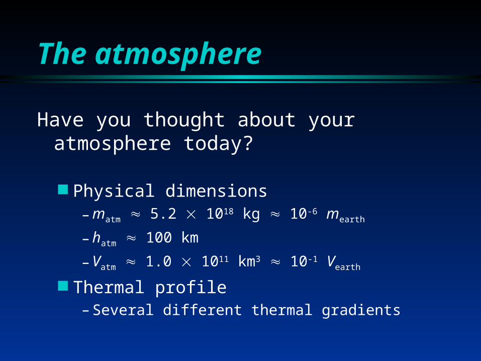
The atmosphere
Have you thought about your atmosphere today?
Physical dimensions– matm 5.2 1018 kg 10-6 mearth
– hatm 100 km
– Vatm 1.0 1011 km3 10-1 Vearth
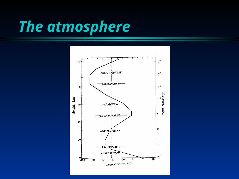
Thermal profile– Several different thermal gradients
The atmosphere
The atmosphere
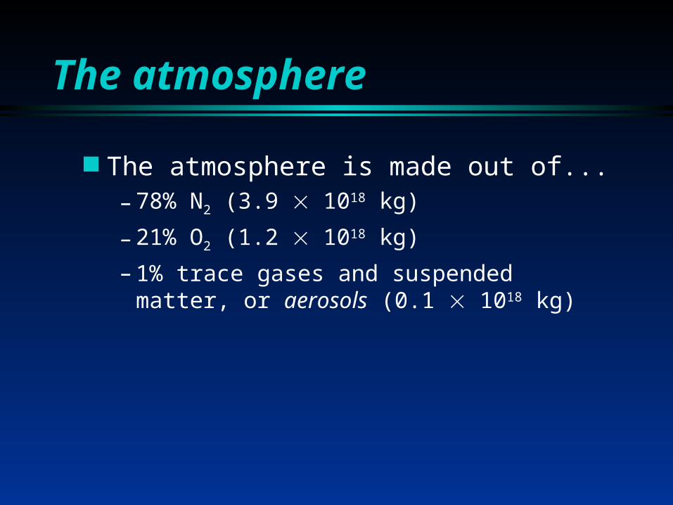
The atmosphere is made out of...– 78% N2 (3.9 1018 kg)
– 21% O2 (1.2 1018 kg)
– 1% trace gases and suspended matter, or aerosols (0.1 1018 kg)

Aerosols
Aerosols
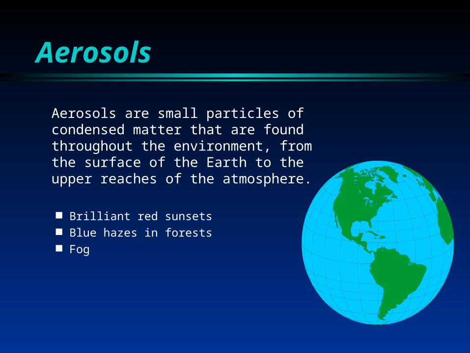
Aerosols are small particles of condensed matter that are found throughout the environment, from the surface of the Earth to the upper reaches of the atmosphere.
Brilliant red sunsets Blue hazes in forests Fog

Aerosol characteristics
An aerosol is characterized by Composition Size Phase Shape

Aerosol composition
Organic materials Long-chained hydrocarbons Large carboxylic acids
Inorganic materials Mineral acids Metals
Organic/inorganic mixtures
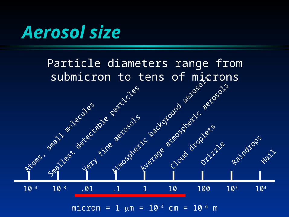
Aerosol size
Particle diameters range from submicron to tens of microns
micron = 1 m = 10-4 cm = 10-6 m
10-4 10-3 .01 .1 1 10 100 103 104
Atom
s, sm
all m
olecu
les
Small
est d
etec
table
par
ticles
Very f
ine a
eros
ols
Atmos
pher
ic ba
ckgr
ound
aer
osols
Avera
ge a
tmos
pher
ic ae
roso
ls
Cloud
drop
lets
Drizzle
Raindr
ops
Hail

Aerosol phase
Liquids Oil droplets from vegetation Sulfuric acid aerosols
Solids Suspended crust material Water ice particles in cirrus clouds
Liquid/solid mixtures
Aerosol shape
Liquids: spherical droplets Solids: crystals and complex structures Shape can impact physical, chemical,
and optical properties of aerosols
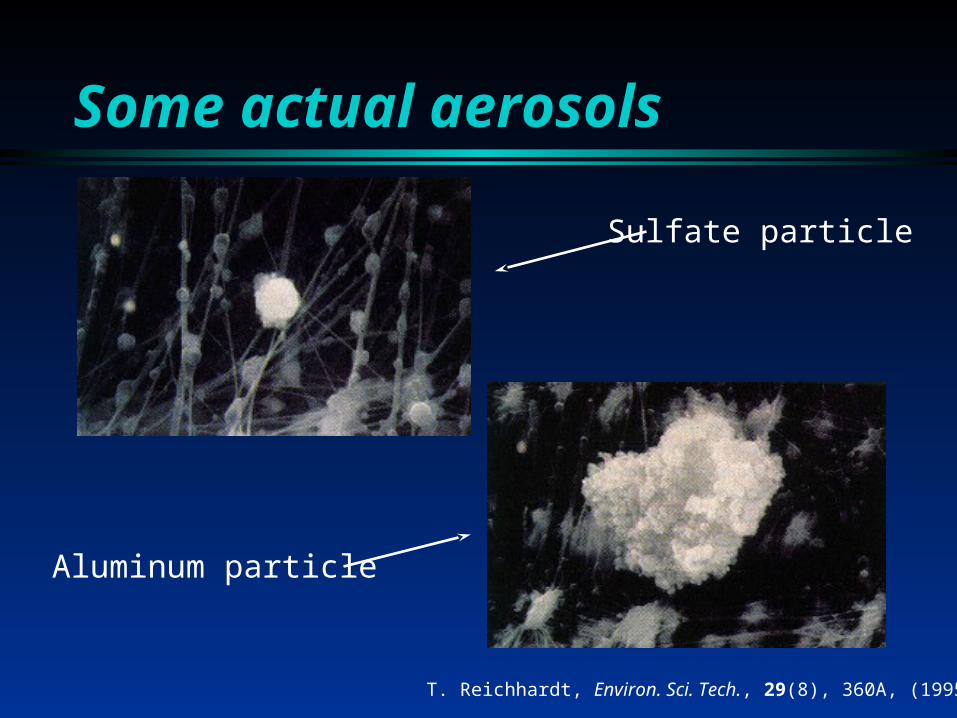
Some actual aerosols
T. Reichhardt, Environ. Sci. Tech., 29(8), 360A, (1995).
Sulfate particle
Aluminum particle
Aerosol sources
Natural sources Vegetation Oceans Volcanoes
Anthropogenic sources Vehicle and industrial emissions Agricultural practices
Aerosol production
Mechanical action Abrasion of plant leaves Sea spray Wind
Nucleation and condensation Cloud formation

Aerosols and the Environment
Aerosols and the Environment
Ozone depletion Global climate change
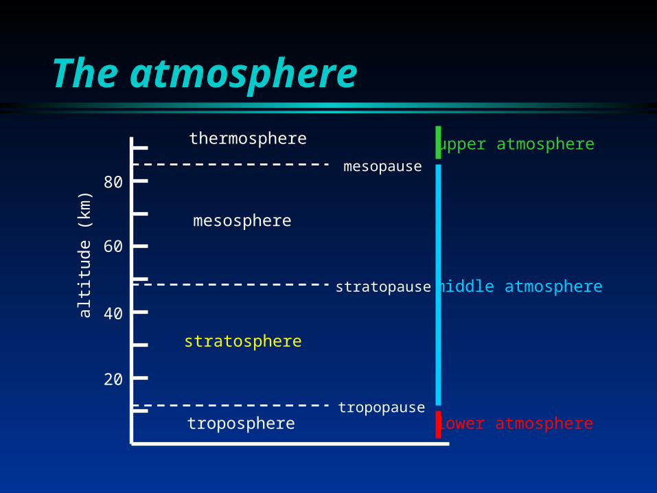
The atmosphereal
titud
e (k
m)
20
40
60
80
tropopause
stratopause
mesopause
stratosphere
mesosphere
thermosphere upper atmosphere
middle atmosphere
lower atmospheretroposphere
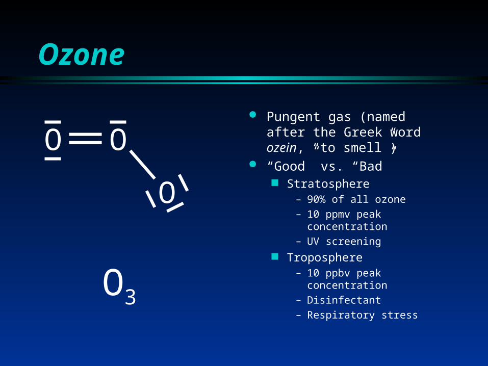
Ozone
O
O O Pungent gas (named after
the Greek word ozein, “to smell”)
“Good” vs. “Bad” Stratosphere
– 90% of all ozone– 10 ppmv peak concentration– UV screening
Troposphere– 10 ppbv peak concentration– Disinfectant– Respiratory stress
O3
Ozone
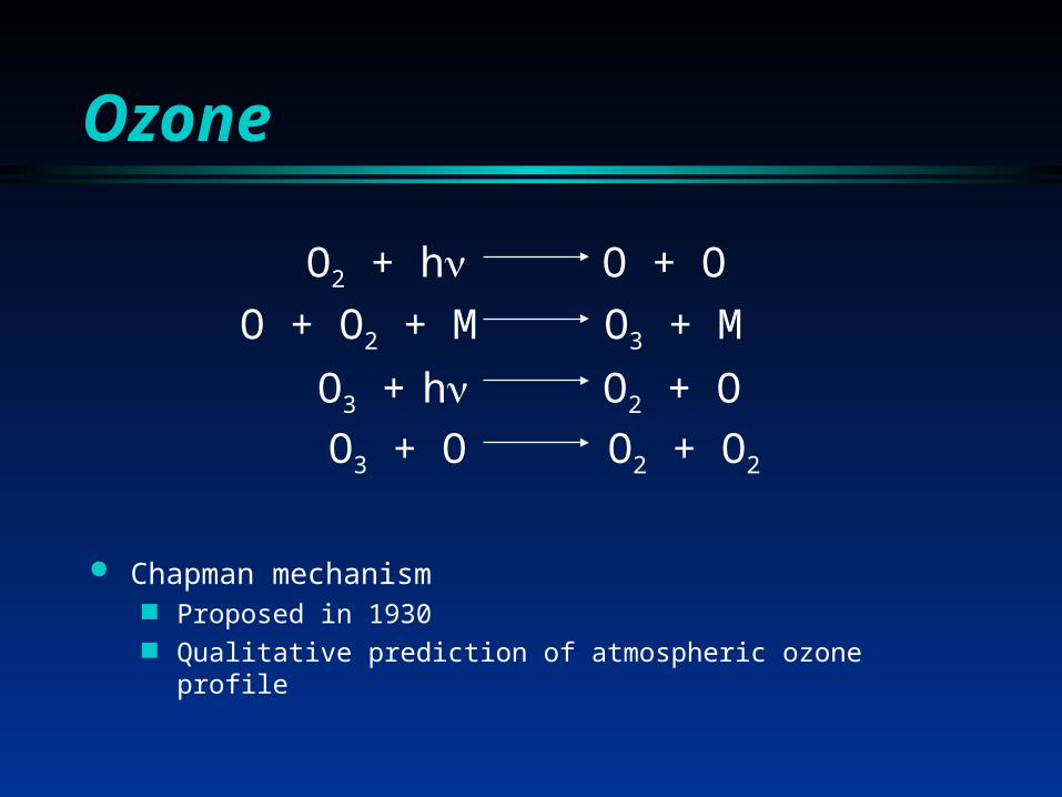
O2 + h O + O
O + O2 + M O3 + M
O3 + h O2 + O
O3 + O O2 + O2
Chapman mechanism Proposed in 1930 Qualitative prediction of atmospheric ozone profile
Ozone depletion
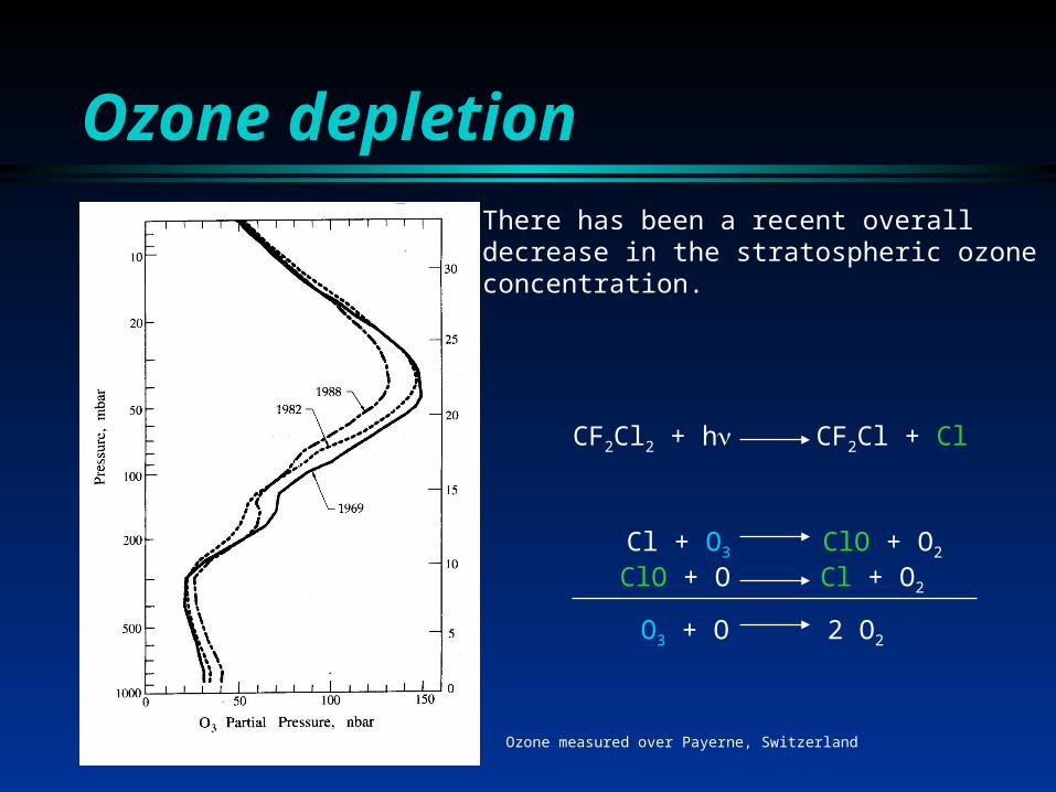
There has been a recent overall decrease in the stratospheric ozone concentration.
Ozone measured over Payerne, Switzerland
CF2Cl2 + h CF2Cl + Cl
Cl + O3 ClO + O2
ClO + O Cl + O2
O3 + O 2 O2
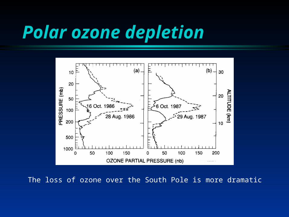
Polar ozone depletion
The loss of ozone over the South Pole is more dramatic
Polar ozone depletion theories
Atmospheric motions Stratospheric air replaced with
tropospheric air
Discounted due to lack of tropospherictrace gases in the stratosphere
Polar ozone depletion theories
Reactive nitrogen species chemically destroy ozone
Discounted due to low concentrations of nitrogen species during depletion events
Polar ozone depletion theories
Chlorine compounds are responsible for the ozone depletion Produced from CFCs Persist for up to 100 years
Polar ozone depletion cycle
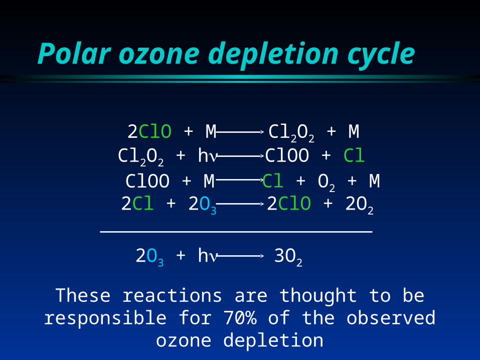
2ClO + M Cl2O2 + MCl2O2 + h ClOO + ClClOO + M Cl + O2 + M2Cl + 2O3 2ClO + 2O2
2O3 + h 3O2
These reactions are thought to be responsible for 70% of the observed ozone depletion

Homogeneous reactions
CFCs
ClONO2
h
ClONO2
h
Polar stratospheric chemistry
Homogenous chemistry cannot provide all of the ClO needed to deplete ozone
Ozone depletion occurs in the presence of polar stratospheric clouds or PSCs

Polar stratospheric clouds
Type I Formed near 195 K Composed of nitric acid and water Exist in different phases
– Type Ia: Solid nitric acid particles– Type Ib: Supercooled liquid droplets (sulfuric acid,
nitric acid, water)
Type II Formed near 185 K Water ice particles

Heterogeneous reactions
ClONO2(s) + HCl(s) Cl2(g) + HNO3(s)
ClONO2(s) + H2O(s) HOCl(g) + HNO3(s)
Chlorine is released into the gas phase Nitrogen is chemically removed Nitrogen is physically removed
PSCs
PSCs
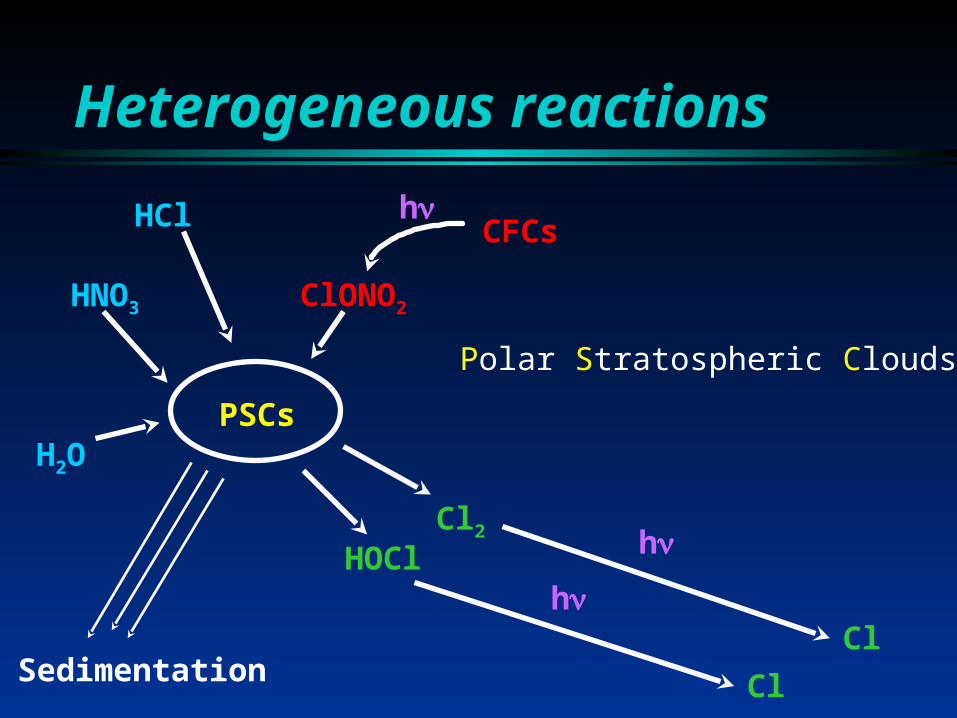
Heterogeneous reactions
CFCs
ClONO2
h
PSCs
HCl
HNO3
Sedimentation
Cl2
H2O
Polar Stratospheric Clouds
HOCl h
hCl
Cl
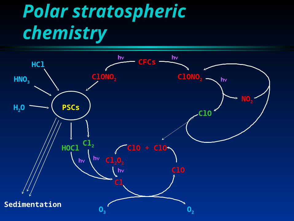
Polar stratospheric chemistry
CFCs
ClONO2ClONO2
ClO
Cl2
NO2
PSCs
HCl
HNO3
Sedimentation
ClO + ClO
Cl2O2
Cl
ClO
O3 O2
h h
h
h
H2O
HOClhh
Polar stratospheric chemistry
Heterogeneous reaction rates are dependent on PSC phase, composition, and size
Need to characterize PSCs to fully investigate depletion process
PSC characterization
Collect infrared spectra of PSCs Mie scattering theory
Spherical particles Complex refractive indices for proposed
PSC components
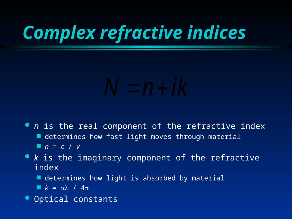
Complex refractive indices
N n ik n is the real component of the refractive index
determines how fast light moves through material n = c / v
k is the imaginary component of the refractive index determines how light is absorbed by material k = / 4
Optical constants

PSC spectra
O.B.Toon and M.A. Tolbert, Nature, 375, 218, (1995).
IceNADNAT
Polar stratospheric clouds
Good fits were not obtained using known optical constants for Water ice Nitric acid monohydrate (NAM): HNO3H2O
Nitric acid dihydrate (NAD): HNO3H2O
Nitric acid trihydrate (NAT): HNO33H2O

Polar stratospheric clouds
PSCs are not pure water or nitric acid aerosols
Ternary mixtures with sulfuric acid Determine optical constants for ternary
mixtures
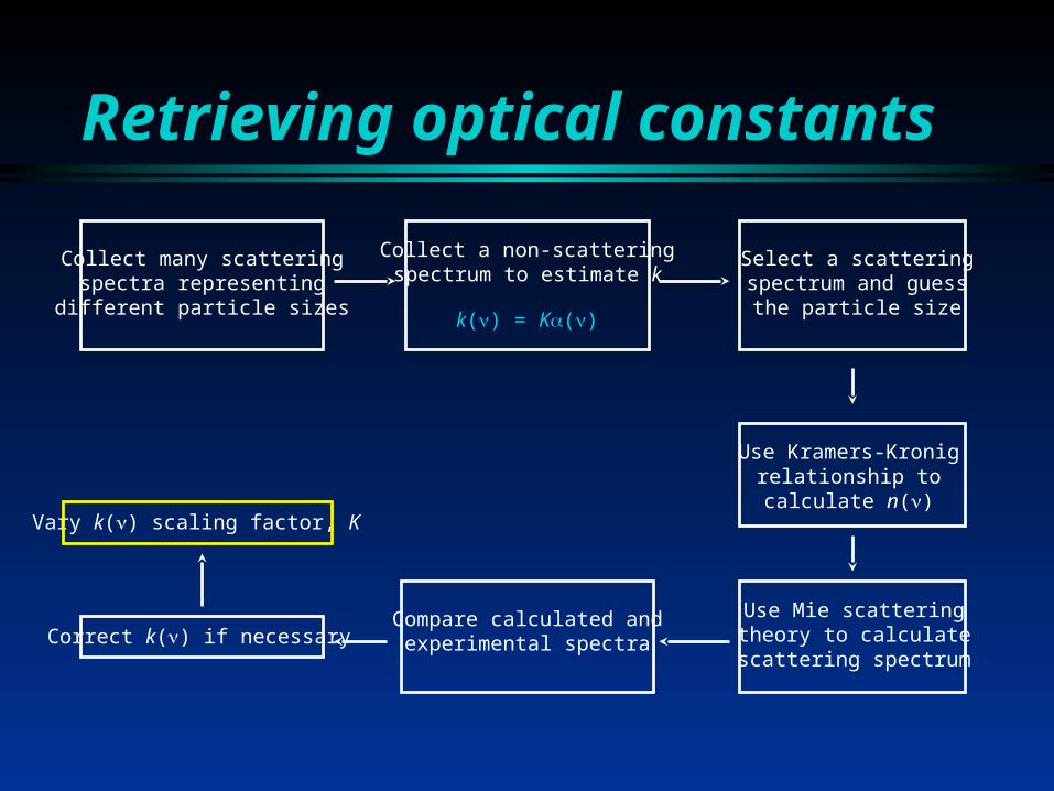
Retrieving optical constants
Retrieve optical constants from infrared spectra of model PSC aerosols Frequency Temperature
Optical constants for NAD
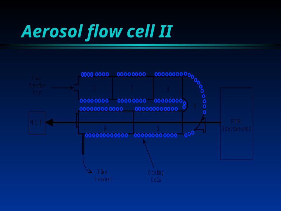
Aerosol flow cell II
F l o wIn je c t io n
P o r t
F T I RS p e c t ro m e te r
F l o wE x h a u s t
C o o l in gC o i ls
M C T
1 2 3
4
56
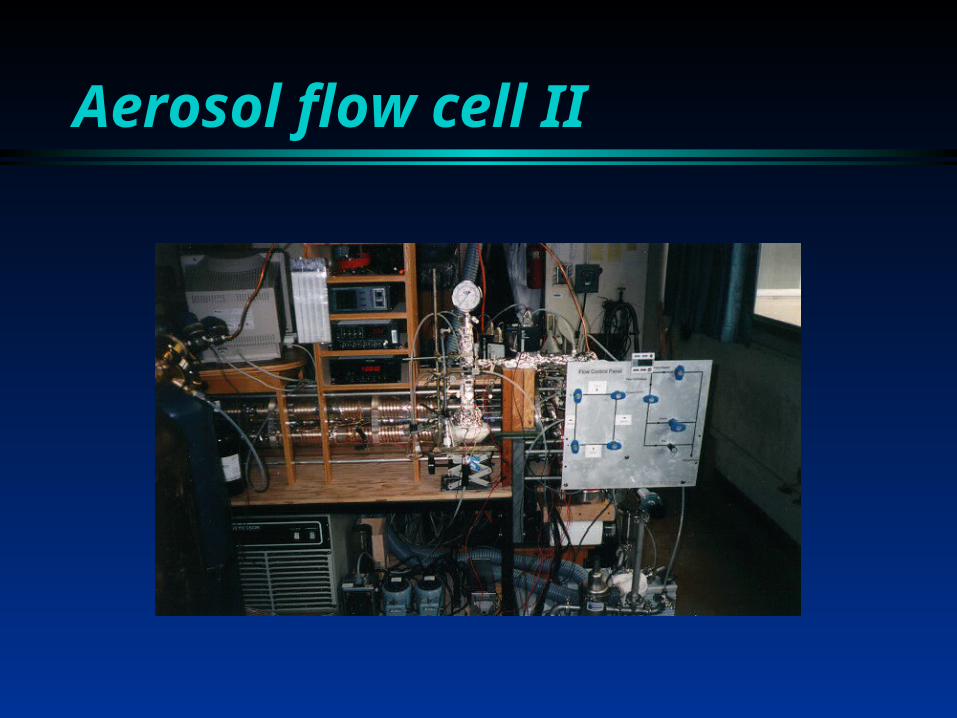
Aerosol flow cell II
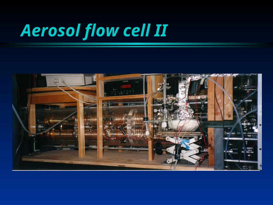
Aerosol flow cell II
Retrieving optical constants
Collect many scatteringspectra representing
different particle sizes
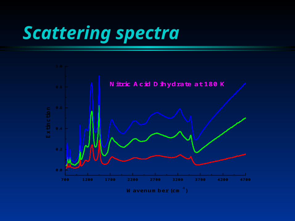
Scattering spectra
700 1200 1700 2200 2700 3200 3700 4200 4700
0.0
0.2
0.4
0.6
0.8
1.0
Nitric Acid Dihydrate at 180 K
Exti
ncti
on
Wavenumber (cm-1)
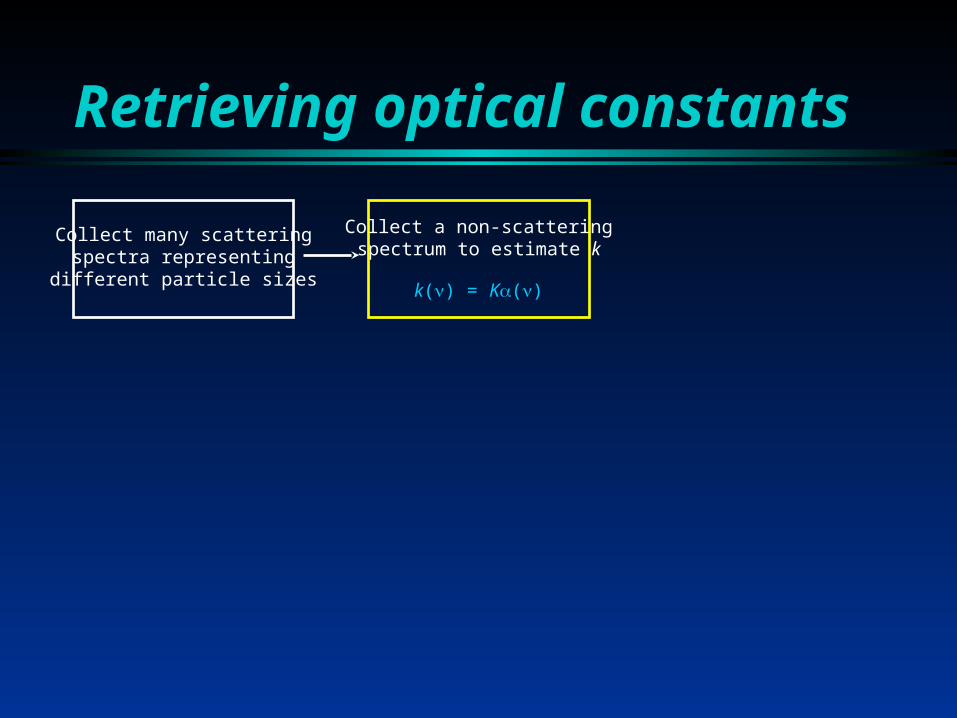
Retrieving optical constants
Collect a non-scatteringspectrum to estimate k
k() = K()
Collect many scatteringspectra representing
different particle sizes

Non-scattering spectrum
700 1200 1700 2200 2700 3200 3700 4200 4700
0.00
0.05
0.10
0.15
0.20
Nitric Acid Dihydrate at 180 K
Exti
ncti
on
Wavenumber (cm-1)
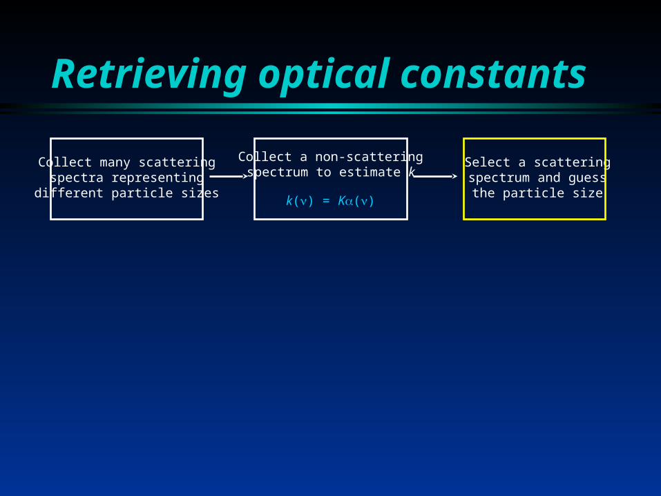
Retrieving optical constants
Select a scatteringspectrum and guess
the particle size
Collect many scatteringspectra representing
different particle sizes
Collect a non-scatteringspectrum to estimate k
k() = K()

Retrieving optical constants
Select a scatteringspectrum and guess
the particle size
Use Kramers-Kronigrelationship tocalculate n()
Collect many scatteringspectra representing
different particle sizes
Collect a non-scatteringspectrum to estimate k
k() = K()

Retrieving optical constants
Select a scatteringspectrum and guess
the particle size
Use Kramers-Kronigrelationship tocalculate n()
Use Mie scatteringtheory to calculate
scattering spectrum
Collect many scatteringspectra representing
different particle sizes
Collect a non-scatteringspectrum to estimate k
k() = K()
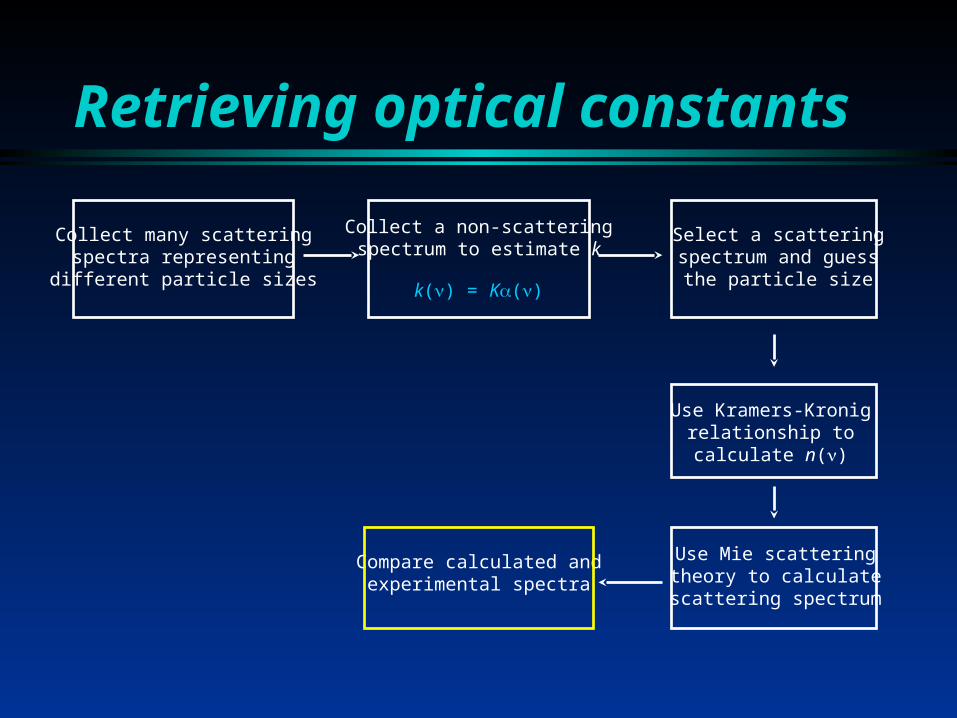
Retrieving optical constants
Select a scatteringspectrum and guess
the particle size
Use Kramers-Kronigrelationship tocalculate n()
Use Mie scatteringtheory to calculate
scattering spectrum
Compare calculated andexperimental spectra
Collect many scatteringspectra representing
different particle sizes
Collect a non-scatteringspectrum to estimate k
k() = K()
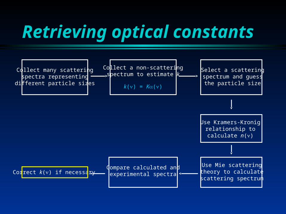
Retrieving optical constants
Select a scatteringspectrum and guess
the particle size
Use Kramers-Kronigrelationship tocalculate n()
Use Mie scatteringtheory to calculate
scattering spectrum
Compare calculated andexperimental spectraCorrect k() if necessary
Collect many scatteringspectra representing
different particle sizes
Collect a non-scatteringspectrum to estimate k
k() = K()
Retrieving optical constants
Select a scatteringspectrum and guess
the particle size
Use Kramers-Kronigrelationship tocalculate n()
Use Mie scatteringtheory to calculate
scattering spectrum
Compare calculated andexperimental spectraCorrect k() if necessary
Vary k() scaling factor, K
Collect many scatteringspectra representing
different particle sizes
Collect a non-scatteringspectrum to estimate k
k() = K()
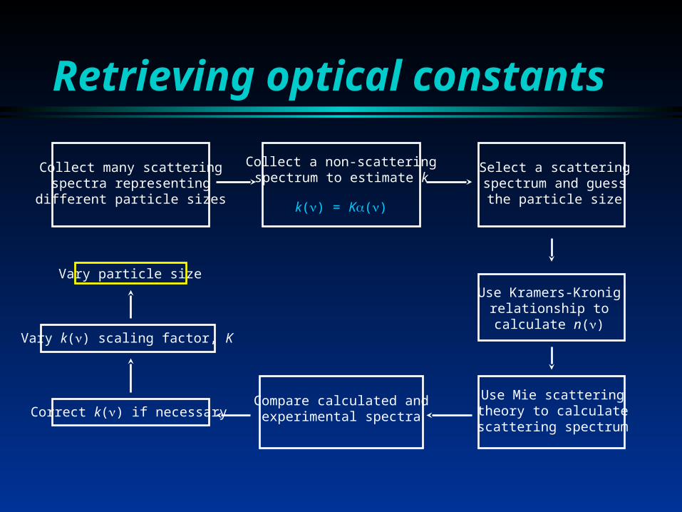
Retrieving optical constants
Select a scatteringspectrum and guess
the particle size
Use Kramers-Kronigrelationship tocalculate n()
Use Mie scatteringtheory to calculate
scattering spectrum
Compare calculated andexperimental spectraCorrect k() if necessary
Vary k() scaling factor, K
Vary particle size
Collect many scatteringspectra representing
different particle sizes
Collect a non-scatteringspectrum to estimate k
k() = K()
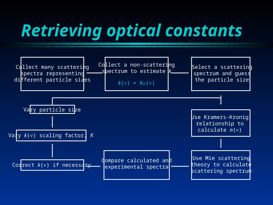
Retrieving optical constants
Select a scatteringspectrum and guess
the particle size
Use Kramers-Kronigrelationship tocalculate n()
Use Mie scatteringtheory to calculate
scattering spectrum
Compare calculated andexperimental spectraCorrect k() if necessary
Vary k() scaling factor, K
Vary particle size
Collect many scatteringspectra representing
different particle sizes
Collect a non-scatteringspectrum to estimate k
k() = K()
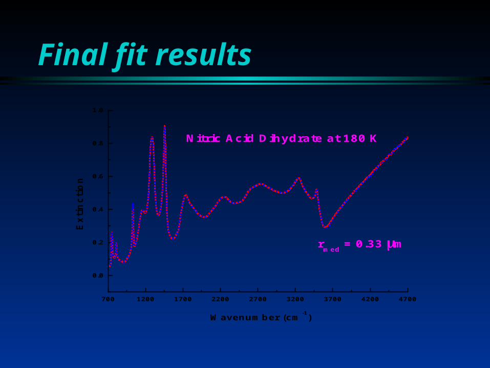
Final fit results
700 1200 1700 2200 2700 3200 3700 4200 4700
0.0
0.2
0.4
0.6
0.8
1.0
rmed
= 0.33 m
Nitric Acid Dihydrate at 180 K
Exti
ncti
on
Wavenumber (cm-1)
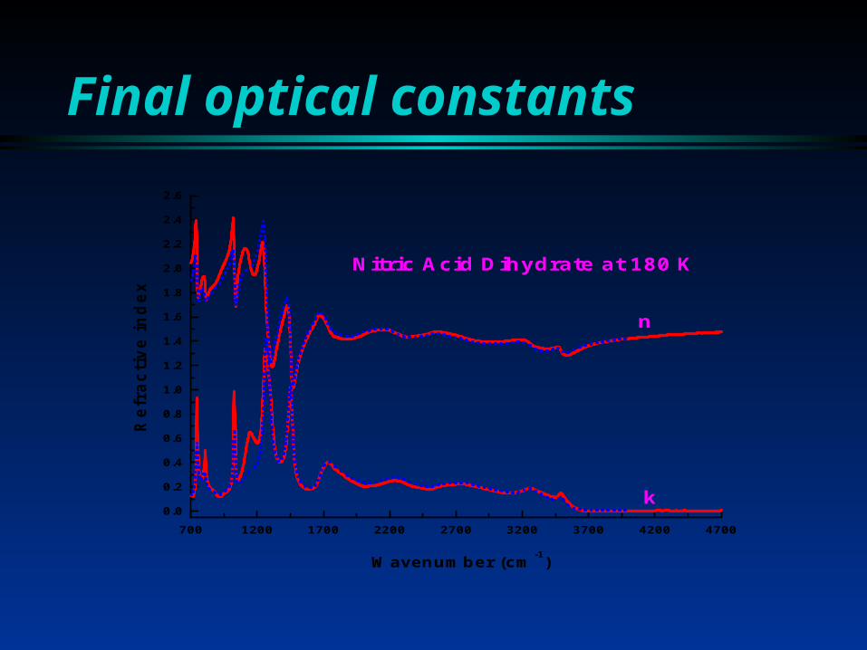
Final optical constants
700 1200 1700 2200 2700 3200 3700 4200 4700
0.0
0.2
0.4
0.6
0.8
1.0
1.2
1.4
1.6
1.8
2.0
2.2
2.4
2.6
k
n
Nitric Acid Dihydrate at 180 K
Refr
acti
ve in
dex
Wavenumber (cm-1)
NAD optical constants
Overall good agreement with thin-film results
Some discrepancies do exist Comparison of several aerosol and thin-
film spectra suggest substrate interference
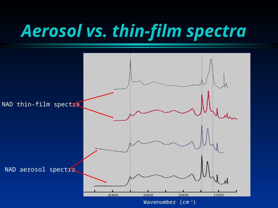
Aerosol vs. thin-film spectra
NAD thin-film spectra
NAD aerosol spectra
Wavenumber (cm-1)
Aerosol optical constants
Optical constants derived from aerosols arebetter suited for analyzing atmospheric particles

Aerosol composition
NAD aerosols have a fixed composition Composition of liquid sulfuric acid
aerosols can vary
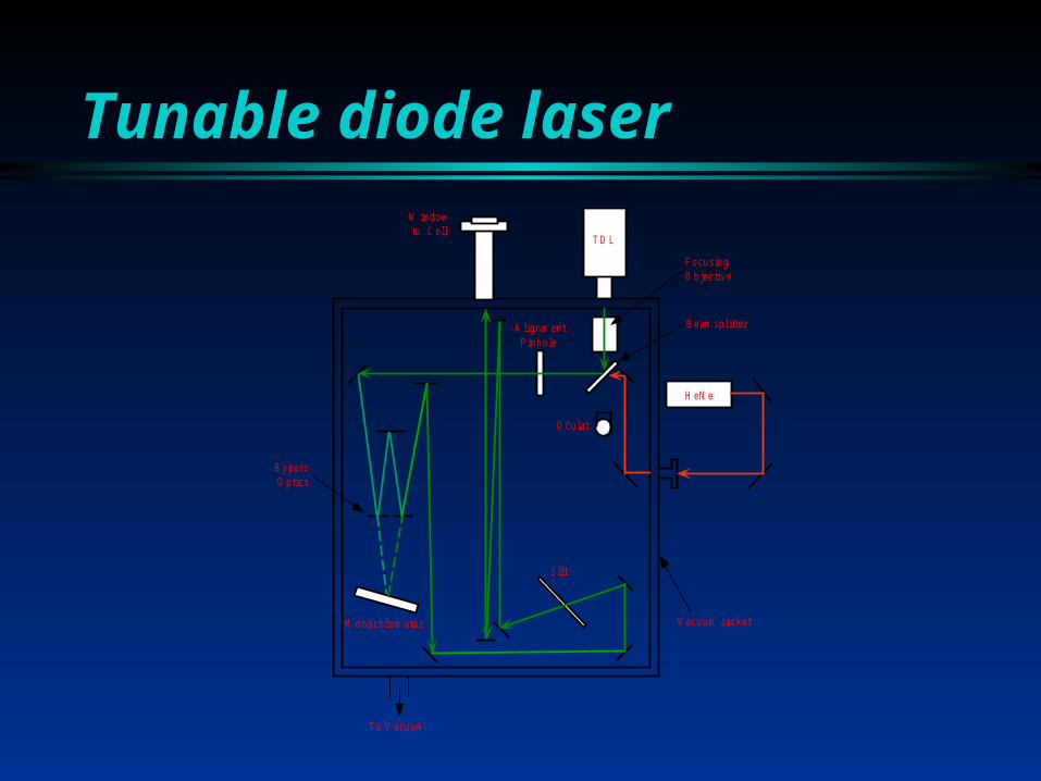
Tunable diode laser
H eN e
T D L
T o V acuum
W indow to C ell
F ocusingO bjective
B eam splitterA lignm ent P inho le
O cular
S lit
B ypass O ptics
M onochrom ator V acuum Jacket
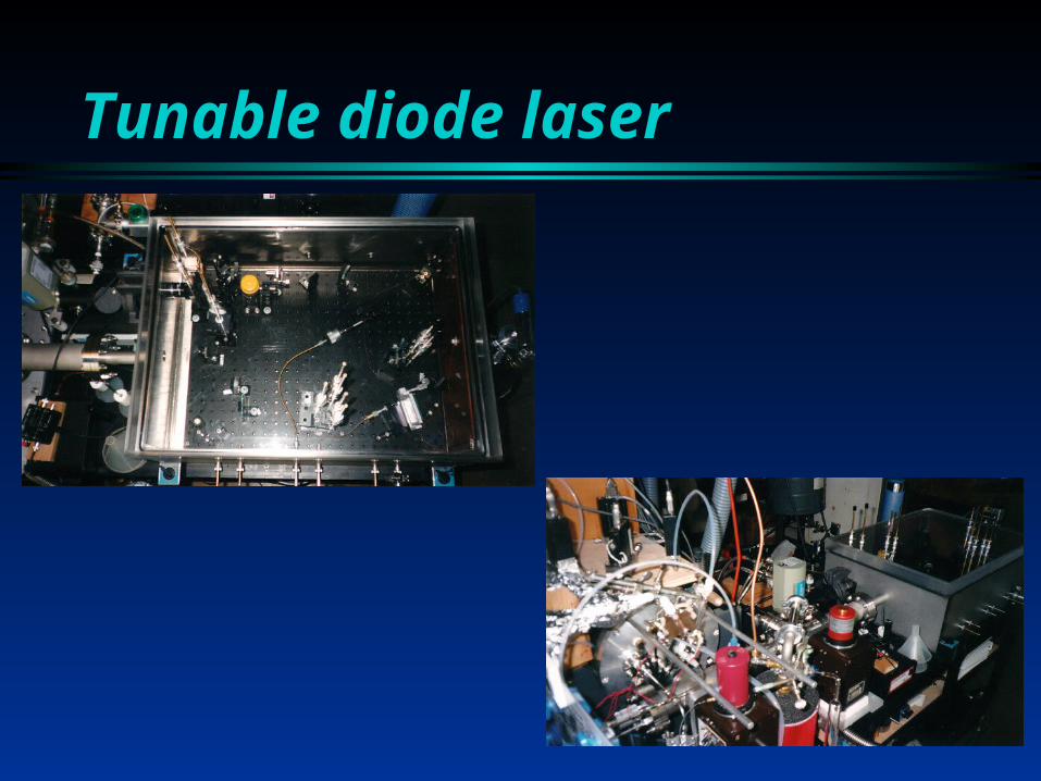
Tunable diode laser
Tunable diode laser
Diode laser beam samples the same aerosol stream as the FT-IR spectrometer
Determines water vapor pressure by applying Beer’s law to a single water absorption line
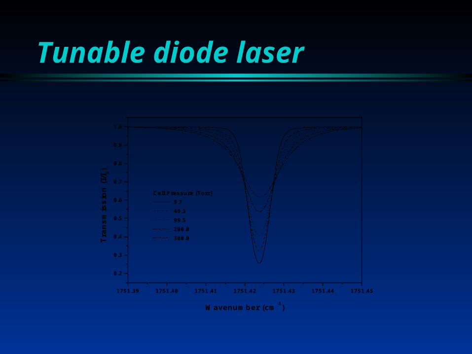
Tunable diode laser
1751.39 1751.40 1751.41 1751.42 1751.43 1751.44 1751.45
0.2
0.3
0.4
0.5
0.6
0.7
0.8
0.9
1.0
Cell Pressure (Torr) 9.7 49.3 99.5 200.0 300.0T
ran
smis
sio
n (
I/Io)
Wavenumber (cm-1)
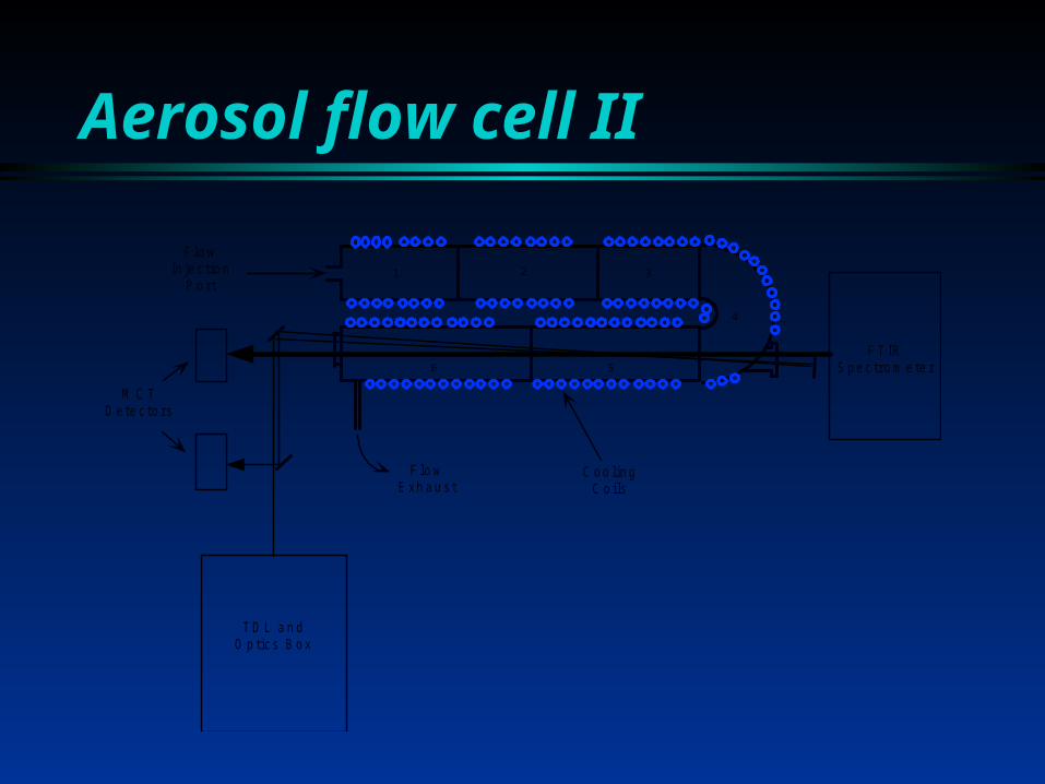
Aerosol flow cell II
F l o wIn je c t io n
P o r t
F T I RS p e c t ro m e te r
M C TD e te c to rs
F l o wE x h a u s t
1 2 3
C o o l in gC o i ls
T D L a n dO p t ic s B o x
4
56
Sulfuric acid optical constants
One optical constant study by Palmer and Williams in 1975
Bulk data for a few concentrations at room temperature
Widely used by atmospheric scientists Spectra change substantially at low
temperatures

Sulfuric acid optical constants
800 1300 1800 2300 2800 3300 3800 4300
0.0
0.2
0.4
0.6
0.8
1.0
1.2
1.4
1.6
1.8
2.0
2.2
2.4
2.6
75 wt% Sulfuric Acid/Water
k
n
Refr
acti
ve In
dex
Wavenumber (cm-1)
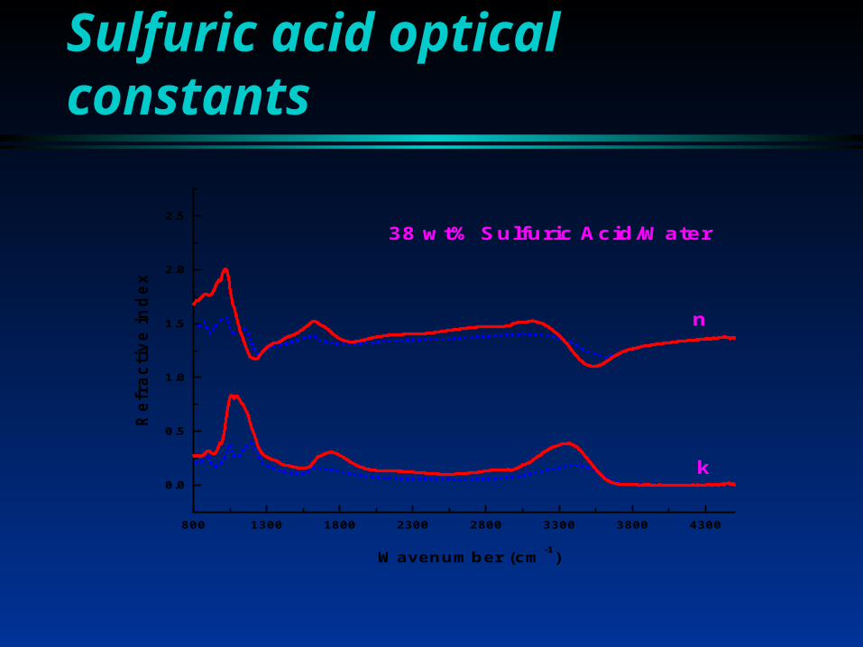
Sulfuric acid optical constants
800 1300 1800 2300 2800 3300 3800 4300
0.0
0.5
1.0
1.5
2.0
2.5
k
n
38 wt% Sulfuric Acid/Water
Refr
acti
ve in
dex
Wavenumber (cm-1)
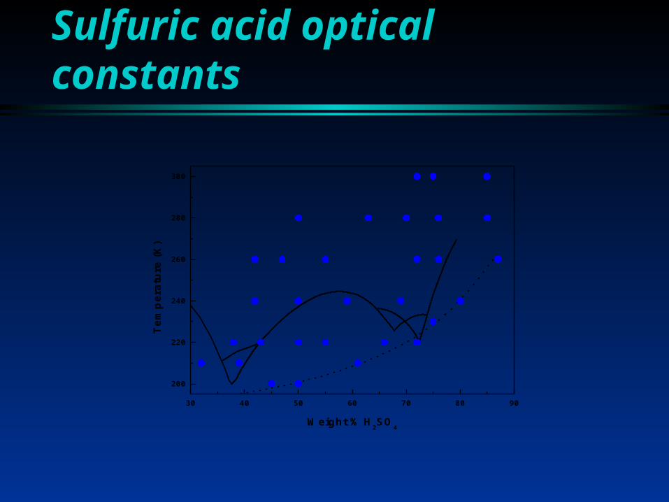
Sulfuric acid optical constants
30 40 50 60 70 80 90
200
220
240
260
280
300
Tem
per
atu
re (
K)
Weight % H2SO
4

Sulfuric acid optical constants
The Palmer and Williams optical constants should not be used at low temperatures
Temperature and composition dependence indicate interesting ion equilibrium chemistry
Emphasize the need to perform similar studies on ternary systems

Aerosols and the Environment
Ozone depletion Global climate change

The atmosphereal
titud
e (k
m)
20
40
60
80
tropopause
stratopause
mesopause
stratosphere
mesosphere
thermosphere upper atmosphere
middle atmosphere
lower atmospheretroposphere
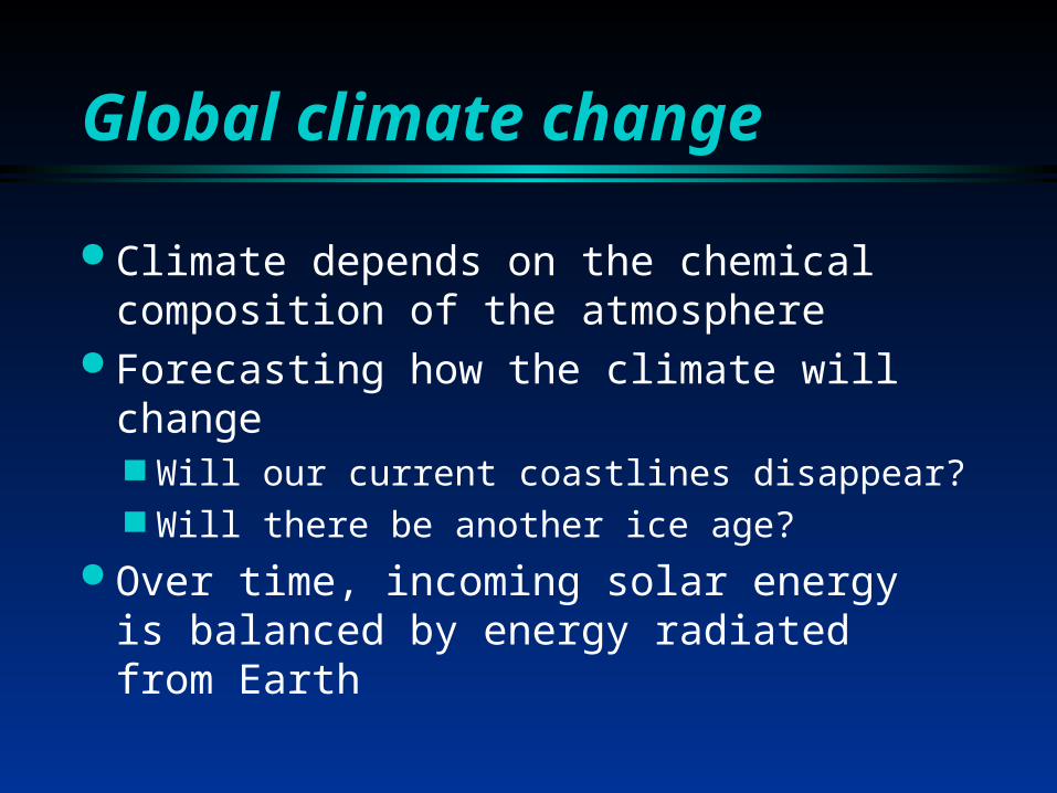
Global climate change
Climate depends on the chemical composition of the atmosphere
Forecasting how the climate will change Will our current coastlines disappear? Will there be another ice age?
Over time, incoming solar energy is balanced by energy radiated from Earth
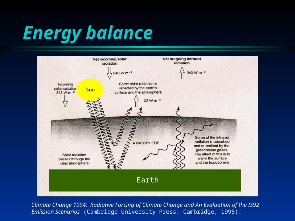
Energy balance
Climate Change 1994: Radiative Forcing of Climate Change and An Evaluation of the IS92Emission Scenarios (Cambridge University Press, Cambridge, 1995).
Eath
Sun
Earth
Energy imbalance
Anything which causes a change in the energy balance is known as a forcing
Climate responds to forcing by re-establishing energy balance
A forcing example
Doubling CO2 concentration Forcing of 4 Wm-2
Surface must warm up 1 Kto restore balance
Positive forcing warms the planet,while negative forcing cools the planet
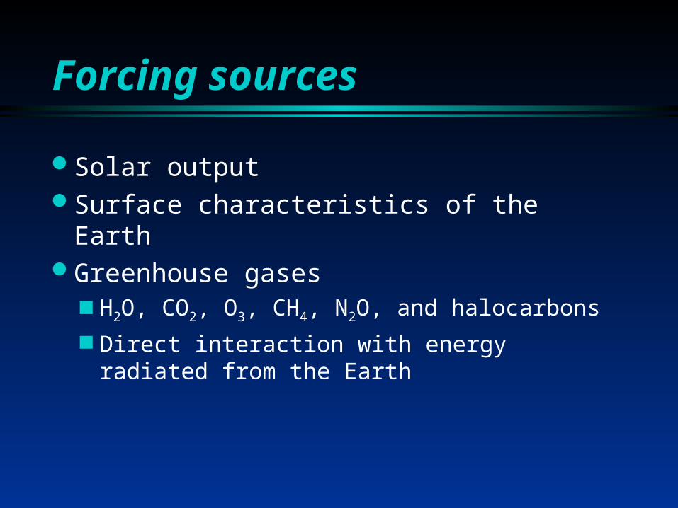
Forcing sources
Solar output Surface characteristics of the Earth Greenhouse gases
H2O, CO2, O3, CH4, N2O, and halocarbons
Direct interaction with energy radiated from the Earth
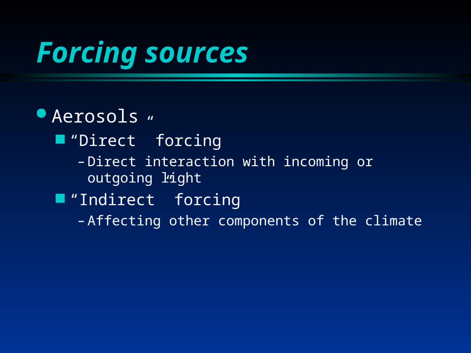
Forcing sources
Aerosols “Direct” forcing
– Direct interaction with incoming or outgoing light
“Indirect” forcing– Affecting other components of the climate
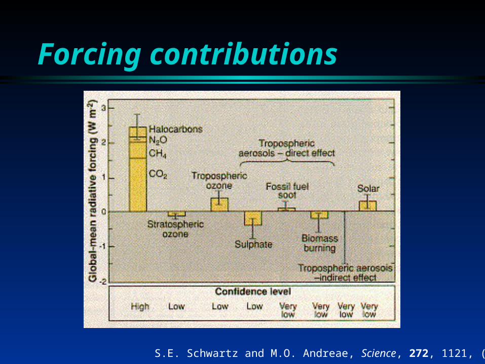
Forcing contributions
S.E. Schwartz and M.O. Andreae, Science, 272, 1121, (1996).

Aerosol forcing uncertainties
Interaction with light is largely unknown Lack of optical constant information
Hygroscopic properties are unknown Important gauge of indirect effects
Complex spatial and temporal distributions throughout the atmosphere
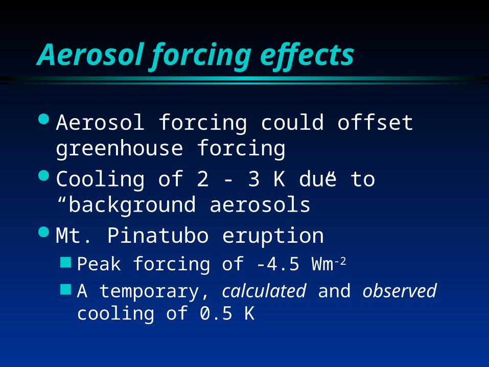
Aerosol forcing effects
Aerosol forcing could offset greenhouse forcing
Cooling of 2 - 3 K due to “background aerosols”
Mt. Pinatubo eruption Peak forcing of -4.5 Wm-2
A temporary, calculated and observed cooling of 0.5 K
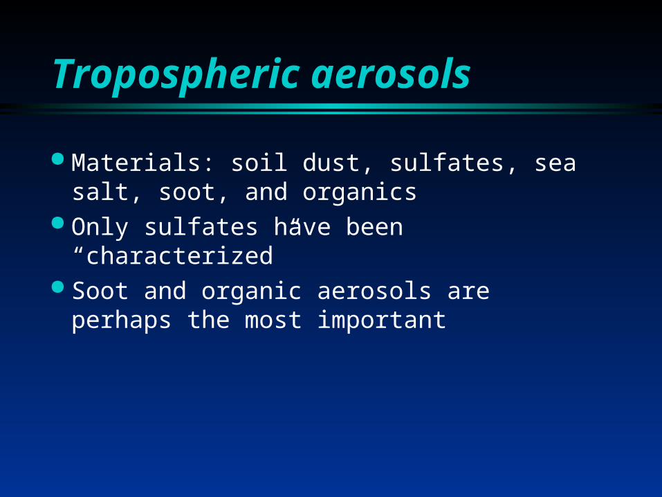
Tropospheric aerosols
Materials: soil dust, sulfates, sea salt, soot, and organics
Only sulfates have been “characterized” Soot and organic aerosols are perhaps
the most important

Present laboratory work
Apply optical constant retrieval method to organic aerosols
Study hygroscopic properties of organic aerosols
Characterize multi-component organic aerosols

Organic aerosols
Primary organic aerosols (POAs) Emitted from source as an aerosol
Secondary organic aerosols (SOAs) Condensation of gas-phase species on pre-
existing particles Composed of terpenes, PAHs, alkanes,
and carboxylic acids
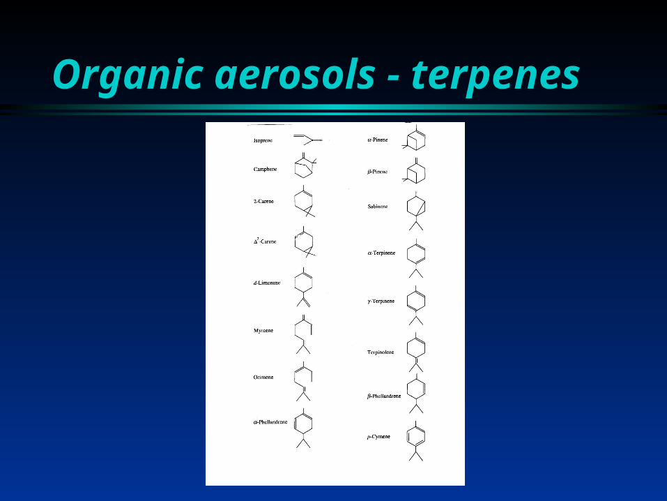
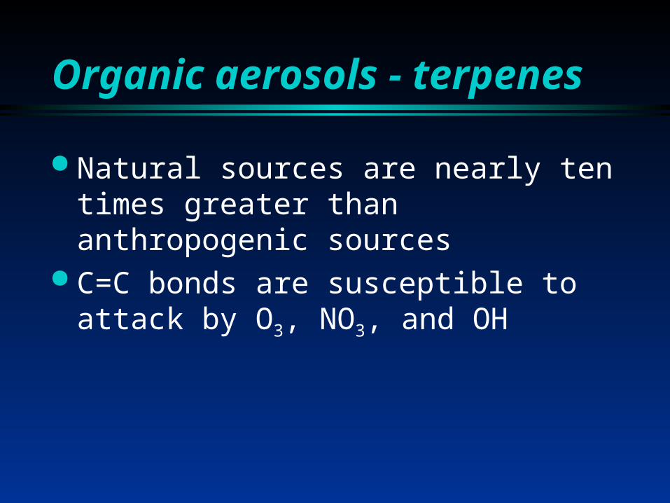
Organic aerosols - terpenes
Organic aerosols - terpenes
Natural sources are nearly ten times greater than anthropogenic sources
C=C bonds are susceptible to attack by O3, NO3, and OH

Model organic aerosols
Determine optical constants for single-component organic aerosols
Start with easily obtained materials that closely represent actual organic aerosols

Model organic aerosols
Carvone1000 2000 3000 4000 5000
0.0
0.5
1.0
1.5
2.0
Abs
orba
nce
Wavenumber (cm-1)
o
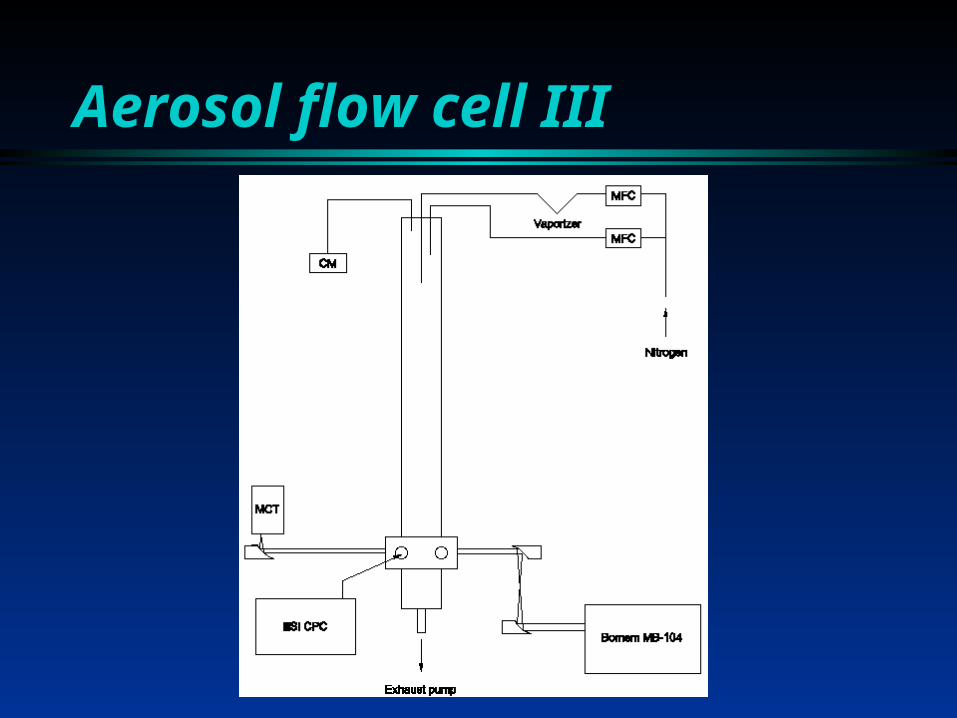
Aerosol flow cell III

Aerosol flow cell III
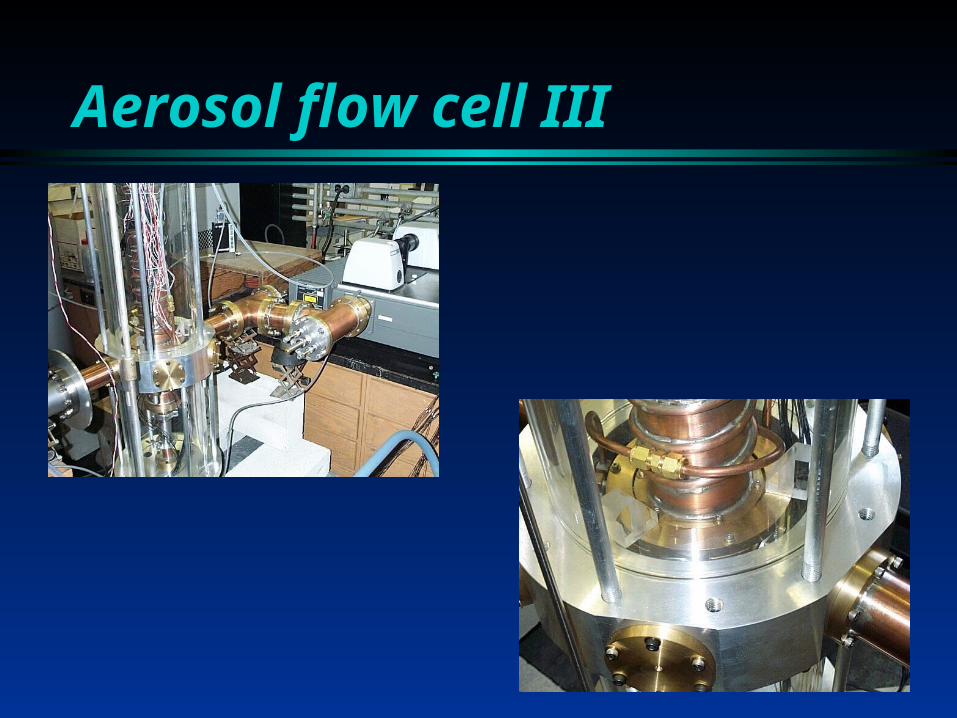
Aerosol flow cell III

First spectra
1000 2000 3000 4000 5000
0.00
0.05
0.10
0.15
0.20
0.25
0.30
0.35
0.40
Abs
orba
nce
Wavenumber (cm-1)
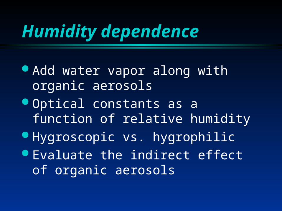
Humidity dependence
Add water vapor along with organic aerosols
Optical constants as a function of relative humidity
Hygroscopic vs. hygrophilic Evaluate the indirect effect of organic
aerosols

Multi-component aerosols
Prepare known mixed organic and mixed organic/inorganic aerosols
Use single-component optical constants to determine refractive index mixing rules
Test rules on unknown aerosols Apply rules to real tropospheric aerosols
Acknowledgments
PSCs (UNC - Chapel Hill) R.E. Miller, D.R. Worsnop, and M.L. Norman NASA Upper Atmosphere Research Program
Organic aerosol studies (DePaul University) Elena Lucchetta LA&S Summer Research Program (1999)