The Causal Effect of Mortgage Refinancing on InterestRate Volatility: Empirical Evidence and Theoretical

Implications

Jefferson Duarte∗

Forthcoming, Review of Financial Studies

∗University of Washington, Box 353200, Seattle WA 98195-3200, e-mail: jduarte@u.washington.edu,phone: (206) 543-1843. I would like to thank Yacine Aït-Sahalia, Eduardo Canabarro, Bing Han, AlanHess, Jon Highum, Avi Kamara, Jon Karpoff, Arvind Krishnamurthy, Haitao Li, Francis Longstaff,Paul Malatesta, Douglas McManus, Jorge Reis, Ed Rice, Pedro Santa-Clara, José Scheinkman, EduardoSchwartz, Andy Siegel, Ken Singleton, an anonymous referee, as well as seminar participants at the 2004Pacific Northwest Finance Conference, 2005 Allied Social Science Associations meeting, 2006 WHU FixedIncome Conference, Freddie Mac, Seattle University, Simon Fraser University, University of Florida andUniversity of Washington for valuable comments. All errors are mine.

1

Abstract

This paper investigates the effects of mortgage-backed security (MBS) hedging activity

on interest rate volatility and proposes a model that takes these effects into account. An

empirical examination suggests that the inclusion of information about MBSs considerably

improves model performance in pricing interest rate options and in forecasting future

interest rate volatility. The empirical results are consistent with the hypothesis that MBS

hedging affects both the interest rate volatility implied by options and the actual interest

rate volatility. The results also indicate that the inclusion of information about the MBS

universe may result in models that better describe the price of fixed-income securities.

2

The effect of mortgage-backed security (MBS) hedging activity on the volatility of

interest rates has been a topic of strong interest among practitioners and policy-makers in

the last few years [e.g., Greenspan (2005a)]. The large size of the MBS market combined

with record home-ownership levels imply that a better understanding of whether there is

a relationship between MBS hedging activity and interest rate volatility may have deep

and broad consequences.

At least three different theories explain the possible relationship between MBS hedging

activity and interest rate volatility. The first theory is based on the hypothesis that the

fixed-income market is perfect and complete without MBSs, and implies that there is no

relationship between MBS hedging activity and interest rate volatility. The second theory

asserts that the dynamic hedging activity of MBS hedgers on the swap and Treasury

markets increases the volatility of interest rates. The third theory assumes that interest

rate option markets are imperfect and that the surge in demand for interest rate options in

a refinancing wave should therefore increase the volatility implied by interest rate options,

such as swaptions.1 This paper empirically analyzes these three theories.

The first theory, which we will call the "classic theory," is based on traditional MBS-

pricing models. These models assume that MBSs are derivatives of the Treasury term

structure [e.g., Schwartz and Torous (1989)]. In these models, as in the Black and Scholes

(1973) model, the activity of derivative hedgers does not have any effect on the prices of

the underlying asset or its derivatives. These models suppose that Treasury markets are

frictionless and complete. As a result, the hedging of MBS investors does not have any

effect on the price of other fixed-income securities.

The second theory, which we will call the "actual volatility effect," is based on the effect

that MBS dynamic hedging is held to have on the Treasury or swap markets. Suppose,

for example, that a mortgage investor holds a portfolio of MBSs and hedges the portfolio

duration risk completely with a short position in Treasury bonds. If interest rates drop,

the mortgage duration decreases due to a higher probability of refinancing. As a result,

the investor will have a portfolio with negative duration. To adjust its duration back to

1Swaptions are options to enter into a plain-vanilla fixed versus floating swap at a certain future dateand at a certain fixed rate. For instance, a payer in a three into seven at-the-money swaption will havethe right (not the obligation) to be the fixed payer in a seven-year swap, three years after the issuance ofthe swaption. Here, the time-to-maturity of the swaption is three years and the tenor of the swaption isseven years. The swaption is at-the-money and hence the agreed upon swap rate is the relevant forwardswap rate at the swaption creation.

3

zero, the investor must buy Treasury bonds. If, on the other hand, interest rates increase,

the mortgage duration increases and the MBS investor must short additional Treasury

bonds in order to adjust the duration of the portfolio. Notice that provided that bond

prices are affected by flows in the Treasury market, the MBS hedging flows (buying bonds

when bond prices are going up and selling bonds when bond prices are going down) will

have the effect of reinforcing both the initial movement of bond prices and their volatility.

The actual volatility effect is similar to that described in the portfolio insurance lit-

erature. Analogous to MBS hedgers, portfolio insurers following a dynamic replication

strategy will sell stocks when stock prices go down and buy stocks when prices go up.

The portfolio insurance literature describes this hedging activity and provides theoretical

models in an incomplete market setting wherein the portfolio insurers’ hedging increases

the volatility of stock prices.2 In these models, the demand for the underlying security

is downward-sloped and the underlying security prices are therefore affected by the flows

generated by portfolio insurers.

The third theory is based on the effect of the static hedging activity of MBS investors

on the interest rate options market, which we will call herein the "implied volatility effect."

MBS investors buy portfolios of loans with embedded call options that allow homeowners

to prepay. An MBS investor may therefore statically hedge the prepayment options with

over-the-counter interest rate options, such as swaptions. Due to the hedging activity of

MBS investors, intense mortgage refinancing activity results in a surge in the demand

for at-the-money interest rate options. That is, when interest rates drop, homeowners

exercise their deep-in-the-money prepayment options and take new mortgages with new

at-the-money prepayment options. These new mortgages are hedged by MBS investors

with new at-the-money interest rate options. As a result, if the supply of options is not

perfectly elastic, a surge in the demand for options caused by an increase in mortgage

refinancing will increase the implied volatility of swaptions.

The implied volatility effect is similar to that described in the limits to arbitrage

literature in the stock options market. The implied volatility effect is analogous to the re-

lationship between shocks in the demand for S&P 500 options and their implied volatility.

In both cases, market imperfections coupled with increases in the demand for options re-

2See, for instance, Grossman (1988), Gennotte and Leland (1990), and Brunnermeier (2001).

4

sult in increases in the options’ implied volatility. That is, market imperfections preclude

option market makers from hedging perfectly, and thus, options market makers charge

higher prices for carrying larger imbalanced inventories of options. As a result, the supply

of options is not perfectly elastic and implied volatility increases with rightward shocks

to options demand.3

Note that these three theories have distinct implications. The implied volatility effect

states that increases in mortgage refinancing should not affect the actual volatility of

interest rates, but it should affect the swaptions’ implied volatility because of the surge in

demand for swaptions during a refinancing wave. The actual volatility effect implies that

increases in mortgage refinancing should increase both actual and implied interest rate

volatility, because increases in refinancing activity make the duration of mortgages more

sensitive to interest changes, and MBS dynamic hedging flows are therefore larger during

periods of high refinancing activity. The classic theory implies that hedging activity does

not have any effect on the volatility of the underlying securities and that refinancing

should therefore not have any effect on the volatility of interest rates.

To differentiate between the classic theory and the other two effects, a vector autore-

gressive (VAR) system is estimated. The results of the VAR indicate that increases in

refinancing activity forecasts increases in interest rate volatility even after controlling for

the level and slope of the term structure. The results are in agreement with the results

in Perli and Sack (2003), even though their econometric framework is different from the

one used here. The results of the VAR are evidence against the classic theory.

To differentiate between actual and implied volatility effects, this paper proposes

and calibrates a term-structure model that incorporates information about MBS pre-

payments. This paper is the first to propose and empirically examine a term-structure

model that incorporates mortgage prepayment information. The proposed term-structure

model with mortgage refinancing effects is called the MRE model and it is an extension

of the Longstaff, Santa-Clara, and Schwartz (2001) model, or LSS model.

The MRE model is a non-arbitrage model based on empirical relationships justified

with the presence of limits to arbitrage. The MRE model is a reduced-form model in the

3See, for instance, Froot and O’Connell (1999), Bollen and Whaley (2004), and Gârleanu, Pedersenand Poteshman (2005).

5

sense that it abstracts from the possible causes for the relationship between interest rate

volatility and mortgage refinancing and takes this relationship as a given. The MREmodel

therefore does not explain the reasons for the possible relationship between refinancing

and interest rate volatility. The MRE model, however, is flexible enough to price fixed-

income derivatives, including swaptions with different tenors and times-to-maturity. The

flexibility of the MRE model makes it a useful tool with which to analyze how, or whether

mortgage refinancing affects the prices of interest rate derivatives with different maturities

and payoffs, thereby ultimately providing a deeper understanding of the effects of mortgage

refinancing on interest rate derivatives.

To differentiate between actual and implied volatility effects, the MRE model is used

to forecast future actual interest rate volatility. If refinancing affects only the implied

volatility of swaptions and not the actual volatility of interest rates, the inclusion of mort-

gage effects in a swaption pricing model will improve the model’s ability to fit swaption

prices, but not the model’s ability to forecast the future actual volatility of interest rates.

If, on the other hand, refinancing equally affects both the actual and the implied volatility,

then the implied volatility calculated by the model with refinancing effects should be an

unbiased forecast of the actual future volatility of interest rates. The empirical analysis

of the MRE model indicates that the inclusion of refinancing effects on the swaption pric-

ing model improves the model’s ability to forecast future interest rate volatility, implying

that mortgage refinancing affects the actual volatility of interest rates. The volatilities

implied by the MRE model, however, are not unbiased forecasts of the actual interest rate

volatility. Consequently, the implied volatility effect cannot be completely discarded.

The remainder of this paper is organized as follows: Section 1 describes different

types of mortgage-related securities and investors. Section 2 describes the data used in

this paper. Section 3 presents a VAR examination of the empirical relationship between

the implied volatility of short-term swaptions, the yield curve, and mortgage refinancing.

Section 4 presents all of the calibrated term-structure models. Section 5 presents in-sample

and out-of-sample comparisons of the calibrated models. Section 6 concludes.

6

1. Types of Mortgage-related Securities and Investors

The residential MBSs may be divided between agency and non-agency MBSs. The agency

sector consists of MBSs created through the securitization of residential mortgages by

government-sponsored enterprises (GSEs) such as Fannie Mae and Freddie Mac, as well

as the agency Ginnie Mae. The majority of the securitized residential mortgages in the

United States are securitized into agency MBSs. Indeed, Table 1 displays data from Inside

Mortgage Finance (2004) on the amount of outstanding agency and non-agency mortgage-

related security holdings since 1994. Table 1 shows that since 1994, more than 80% of all

securitized residential mortgages in the U.S. are securitized into agency MBSs.

The main risks of the agency MBSs are interest rate risk (duration risk) and prepay-

ment risk. Credit risk is usually not an issue in agency MBSs because in exchange for a

guarantee fee, the GSE itself guarantees that the cash flow payments will be made. In

addition, mortgages are over-collateralized loans and the mortgages securitized by Ginnie-

Mae have the full credit guaranty of the U.S. government. Prepayment risk, on the other

hand, is considerable in MBSs because residential mortgages allow borrowers to prepay

their mortgages, thereby creating uncertainty regarding the timing of the cash flows of

MBSs.4

The prepayment risk is different for different types of mortgage-related securities,

which may be divided in two types regarding the distribution of cash flows to investors.

The first type is a passthrough, which is a MBS that passes all of the interest and prin-

cipal cash flows of a pool of mortgages (after servicing and guarantee fees) to investors.

Table 1 shows that around 70% of the total amount of agency mortgage-related securities

outstanding is composed of passthroughs. The prepayment risk of a passthrough is the

same as the prepayment risk of the underlying pool of mortgages. The second type of

mortgage-related security is a collateralized mortgage obligation (CMO), the cash flows of

which are derived from passthroughs and are distributed to different investors according

to pre-specified rules. Because different CMOs have different cash flow distribution rules,

they are subject to differing prepayment risks. As a result, there are CMOs that have

a smaller exposure to prepayment risk than passthroughs have. CMOs, however, do not

4Even though credit risk is not an issue in agency MBSs, credit events affect the timing of the cashflows of MBSs and hence generate prepayment risk.

7

change the total prepayment risk of the pool of mortgages underlying the CMO classes.

See Fabozzi and Modigliani (1992) on this point.

The prepayment options embedded in passthroughs generate the negative convexity

of these securities. Indeed, a passthrough price is usually a concave function of the level

of interest rates. Since borrowers can refinance their mortgages when interest rates drop,

the upside potential of a passthrough is limited. The price of the passthrough therefore

gets closer to a constant when interest rates drop, creating the negative convexity of

this security.5 Because of its negative convexity, the duration risk of a passthrough is

dynamically hedged by buying bonds when bond prices increase and selling bonds when

bond prices drop, or analogously, by receiving a fixed rate in interest rate swaps when

swap rates drop and paying fixed rate in interest rate swaps when swap rates increase.

To understand the hedging flows generated by a MBS investor, assume that an in-

vestor takes a long position on a passthrough with notional amount nMBS and hedges

the duration risk with nTsy,0 Treasury notes. Take the yield of the Treasury note as a

proxy for the interest rate level and assume that the initial yield is y0. Hence nTsy,0 is

chosen to make the derivative of the portfolio price with respect to the Treasury yield

equal to zero at y0 (or the initial duration of the portfolio equal to zero). Suppose that

the yield of the note instantaneously moves from y0 to y1, and consequently the hedge

needs to be readjusted to drive the duration of the portfolio back to zero. That is, the

MBS investor has to trade in the Treasury notes in order to rebalance the portfolio. The

notional amount of the Treasury note necessary to readjust the duration of the portfolio

is given by the following expression derived in the Appendix:

nTsy,1 − nTsy,0 ≈ −[nMBS × P

00

MBS(y0) + nTsy,0 × P00

Tsy(y0)]

P0Tsy(y1)

× (y1 − y0). (1)

In Equation 1, nTsy,1−nTsy,0 is the notional amount that needs to be traded on the notes

to readjust the duration of the portfolio to zero. The prices of the passthrough and of the

Treasury note are PMBS and PTsy respectively. Because P00

MBS(y0) is usually negative,

the term between brackets in the formula above is normally negative, which implies that

5 If the coupon of a passthrough is much smaller than the current interest rate, then the passthroughprice can be a convex function of the level of interest rates. For plots of passthrough prices as functionsof the level of interest rates, see Boudoukh, Whitelaw, Richardson, and Stanton (1997) and page 329 ofSundaresan (2002).

8

the hedging flows have the opposite sign to that of the change in rates. Therefore, when

the Treasury yield goes up, (y1 − y0) is positive and nTsy,1 − nTsy,0 is negative, which

implies that the duration is adjusted by short selling additional notes. On the other hand,

when the Treasury yield goes down, (y1 − y0) is negative and nTsy,1 − nTsy,0 is positive

and thus the duration is adjusted by buying Treasury notes. Also observe that even if

the duration target of the hedged portfolio were not zero, the size of the hedging flows

would be given by Equation 1. (See the Appendix for proof.) Consequently, as long as the

convexity of the hedged portfolio is negative, the hedging flows on the Treasury notes are

to buy notes when the note price goes up and sell notes when the note price goes down.

Recall that the actual volatility effect is the increase in interest rate volatility due

to the dynamic hedging activity of MBS investors on the Treasury or swap markets.

Equation 1 clarifies the fact that the actual volatility effect is based on the assumption

that the convexity of the marginal mortgage hedger portfolio is negative. To verify this

assumption, it would be necessary to have information about the convexity of the marginal

hedger portfolio, which is not available. The universe of MBSs, however, has negative

convexity and hence, as long as the marginal hedger portfolio is a representative piece of

the MBS universe, it is likely that the marginal hedger portfolio has negative convexity.

For example, in a daily sample of 16,757 Bloomberg option-adjusted convexities of Ginnie

Mae passthroughs with coupons between 5% and 9.5% from November 1996 to February

2005, around 96% of the option-adjusted convexities are negative.

Naturally, the negative convexity of the MBS universe is not sufficient to establish

a link between interest rate volatility and the MBS hedging flows. In fact, if the MBS

hedging flows of MBSs are small in relation to the liquidity provision on the hedging

instrument market, it would be unlikely that any channel between MBS hedging activ-

ity and interest rate volatility would exist. In order to infer the possible relative size of

the MBS-related hedging flows, Table 1 displays data on the amount of interest-bearing

marketable Treasury securities outstanding. The data on the amount of Treasury secu-

rities outstanding are from various issues of the Federal Reserve Bulletin. Note that the

total amount of mortgage-related security holdings is quite large. For instance, between

1994 and 1997, the total amount of mortgage-related securities outstanding was close to

the total amount of Treasury notes outstanding, while between 2000 and 2003, the total

9

amount of mortgage-related securities outstanding was larger than that of marketable

Treasury securities. Table 1 also displays estimates from Inside Mortgage Finance (2004)

of the holdings of mortgage-related securities by two types of investors that are commonly

assumed to be hedgers: MBS dealers and the GSEs.6

The growth and size of the GSEs portfolios are impressive. The GSEs hold more than

15% of the total amount of mortgage-related securities since 1998. GSEs are required to

manage their interest rate exposure and do so by issuing debt and using a series of fixed-

income products such as Treasury securities, swaps, and swaptions. Indeed, as an attempt

to understand the impact of the dealers’ concentration on the over-the-counter interest

rate options markets, staff of the Federal Reserve System conducted interviews with seven

leading bank and non-bank over-the-counter derivative dealers during the summer of 2004

[Federal Reserve (2005) and Greenspan (2005b)]. The dealers indicated that "Fannie Mae

and Freddie Mac together account for more than half of options demand when measured in

terms of the sensitivity of the instruments to changes in interest rate volatility (rather than

notional amounts)." Naturally, the GSEs’ MBS portfolios were smaller in 1994, indicating

that the MBS hedging demand from the GSEs was not as high in the mid 1990s.

The estimates displayed in Table 1 indicate that MBS dealers had around 6% of the

outstanding mortgage-related securities universe in 1994 and, as opposed to the GSEs, the

portfolios of MBS dealers decreased between 1994 and 2003. Dealers typically manage the

duration of their portfolios and they are among the set of investors whose hedging activity

may drive interest rate volatility. Fernald, Keane, and Mosser (1994) estimate that the

size of the dealers’ inventory of passthroughs and CMOs was more than $50 billion in

the 1993-1994 period, while the size of the new five- to ten-year Treasury supplies, for

example, was around $45 billion a quarter during 1993. As such, Fernald, Keane, and

Mosser argue that the size of the MBS dealers’ hedging demand was large enough that it

might have influenced some of the term-structure movements in the 1993-1994 period.

Hedge funds are another class of MBS investors that typically dynamically hedge

their portfolios. Hedge funds’ fixed-income strategies have been described in Lowenstein

(2000) and in Duarte, Longstaff, and Yu (2007). These strategies usually involve the use

of dynamic hedging. Inside Mortgage Finance (2004) estimates that hedge funds’ MBS

6The estimates displayed in Table 1 are similar to the ones in Goodman and Ho (1998, 2004).

10

holding composed up to 9% of the MBS universe in 1994. Naturally, any estimate of hedge

funds’ MBS holdings should be accepted with caution because the data on the holdings of

hedge funds are not public. Perold (1999), however, indicates that the well-known hedge

fund Long-Term Capital Management (LTCM) alone had positions of up to $20 billion

dollars in market value of passthroughs and CMOs between 1994 and 1997, which suggests

that the participation of hedge funds in the MBS market was not trivial in the mid 1990s.

In the same way that the relative importance of the hedge funds, MBS dealers, and

the GSEs on the MBS market changed between 1994 and 2003, the hedge instruments

also changed. For instance, Fernald, Keane, and Mosser (1994) indicate that MBS dealers

most likely used on-the-run Treasury notes for duration hedging in 1993-1994. Moreover,

Goodman and Ho (1998) indicate that the GSEs started relying more on swap-based

products in their hedging activity around 1997, while prior to 1997 the GSEs appear to

have relied more on their own callable debt and Treasuries as hedging instruments. The

switch from Treasury-based to swap-based hedging could also have been driven by the

change in benchmark in the fixed-income market. Fleming (2000), for example, indicates

that due to a decrease in the supply of Treasuries and the flight-to-quality at the end

of 1998, fixed-income hedgers started relying more on swaps to hedge their portfolio

duration. Consequently, it appears that the hedging instrument of the marginal MBS

hedger switched from Treasury-based to swaps-based during the sample period.

MBS hedgers such as hedge funds and MBS dealers invest in CMOs as well as in

passthroughs, and CMOs account for around 30% of the outstanding mortgage-related

securities. Consequently, it is important to understand whether CMOs have an impact on

the total hedging flow generated by MBS hedgers. Unfortunately, it is not clear whether

CMOs would increase or decrease the total hedging activity of MBS investors. On the one

hand, it is possible that CMOs decrease the total amount of hedging because they allow a

multitude of duration exposures appropriate for many different types of investors; on the

other, it might also be the case that CMOs increase the total amount of MBS hedging

activity because the creation of a CMO with stable duration comes at the expense of

creating another CMO with unstable duration.

To understand how the creation of CMOs might increase the total amount of MBS

hedging activity, assume that two CMO classes (CMO1 and CMO2 ) are backed by the

11

cash flows of a passthrough. In this case, the sum of the second derivatives of the CMO

prices with respect to interest rate level satisfy the equation:

nPassthroughP00

Passthrough = nCMO1P00CMO1

+ nCMO2P00CMO2

. (2)

Assume that CMO1 resembles a non-callable bond with slightly positive convexity. In this

case, Equation 2 and the usual negative convexity of passthroughs implies that CMO2

is highly negatively convex. Assume that CMO1 is bought by an investor that does not

dynamically hedge (e.g., a small commercial bank), while CMO2 is bought by an investor

that normally dynamically hedges (e.g., a hedge fund).7 If these assumptions hold true,

the creation of the CMOs could increase hedging activity because the dynamic hedge of

CMO2 may have to be adjusted more often than the underlying passthrough.8

In addition to investors that normally hedge such as MBS dealers, the GSEs, and

hedge funds, the use of hedging by institutions in the mortgage-related business such as

mortgage originators and servicers is also substantial. Federal Reserve (2005) points out

that over-the-counter interest rate derivative dealers indicate that mortgage servicers9 are

the second most important source of demand for over-the-counter interest rate options. A

mortgage servicer performs the administrative tasks of servicing the pool of mortgages in

exchange for a fee, which is a fixed percentage of the outstanding balance of the mortgage

pool and hence servicing rights are subject to prepayment risk. See Goodman and Ho

(2004) for a description of the hedging activity of mortgage servicers and originators.

In summary, the possibility of a link between MBS hedging and interest rate volatility

from 1994 to 2003 cannot be dismissed based on the relative holdings of MBS investors

and on the existence of CMOs. As a result, the relationship between MBS hedging

activity and interest rate volatility has to be studied by means of indirect evidence—that

is by studying the relationship between proxies of MBS hedging activity and interest rate

7 In this example, CMO 2 is the so-called "toxic waste." Gabaix, Krishnamurthy, and Vigneron (2007)note that the success of CMOs creation typically depends on finding investors willing to buy the "toxicwaste" piece. Investors with expertise in dynamic hedging, such as hedge funds are natural buyers of the"toxic waste" piece.

8As in the example above, Fernald, Keane, and Mosser (1994) argue that the CMOs could increasethe hedging flows generated by MBS dealers.

9Large commercial banks in the U.S. are examples of servicers. Inside Mortgage Finance (2004)indicates that four of the five largest mortgage servicers were among the largest commercial banks in theU.S. in 2004.

12

volatility. Ideally, any study trying to establish a link between interest rate volatility and

MBS hedging should be based on a time series of the trading activity of MBS hedgers.

Unfortunately, this kind of data is not available. As a consequence, in order to investigate

the relationship between MBS hedging activity and interest rate volatility, this paper

assumes that the refinancing activity of the mortgage universe is a proxy for both the

negative convexity of the marginal mortgage hedger portfolio (dynamic hedging in the

actual volatility effect) and the demand for swaptions during periods of high refinancing

activity (static hedging in the implied volatility effect). This paper then analyzes the

relationship between interest rate volatility and refinancing activity.

2. Description of Data

In the remainder of this paper, six kinds of data are used: Libor+swap term-structure

data; constant maturity Treasury yields (CMT) data; swaption implied volatilities data;

data on the outstanding amounts, prepayment speeds, and weighted-average coupons of

Ginnie Mae, Fannie Mae, as well as Freddie Mac mortgage pools; the rate on 30-year-

fixed-rate mortgages; and data on the Mortgage Bankers Association (MBA) Refinancing

Index. The MBA Refinancing Index data are from Bloomberg. The data on the mortgage

pools are also from Bloomberg. The Libor+swap rates, the swaption volatilities, and the

mortgage rates are from Lehman Brothers. The CMT data are from the Federal Reserve

Board.

The CMT data are daily from April 8, 1994 to August 29, 2003. The CMT rates

have two, three, four, five, seven, and ten years to maturity. There are 2,351 observations

for each maturity. The rate on a 30-year-fixed-rate mortgage is used as a proxy for the

current mortgage rate (MRt). The mortgage-rate data are weekly (Friday) from January

31, 1992 to August 29, 2003, which is a total of 605 observations.

The Libor rates are the six-month and one-year Libor. The swap rates are the plain-

vanilla fixed versus floating swap rates with two, three, four, five, seven and ten years to

maturity. The Libor/swap rates are the daily closing from July 24, 1987 to August 29,

2003. There are 4,153 observations for each maturity. These rates are used to estimate the

zero-coupon, continuously-compounded yields with a procedure similar to the one used

by Longstaff, Santa-Clara, and Schwartz (2001) and Driessen, Klaassen, and Melenberg

13

(2003). As in Longstaff, Santa-Clara, and Schwartz, the one-year and the six-month dis-

count rates are directly estimated from the six-month and one-year Libor rates. As in

Driessen, Klaassen, and Melenberg, the discount rates for maturities between one and a

half and ten years are estimated by assuming that the price of a zero-coupon bond with

maturity T at time t is exp(P3

i=1 ωi,t(T − t) +P2

j=1 θj,tmax(0, (T − t − 2 × j)), where

the parameters ωi,t, θj,t are estimated by least squares from the swap rates observed at

time t.

By market convention, the swaption prices are displayed as volatilities of the Black

(1976) model, and the dollar prices of the swaptions are calculated by Black’s formula.

The swaption data are composed of a time series of 40 at-the-money swaption volatilities

with time-to-maturity and tenor given by: three and six months, one, two, and three years

into one, two, three, four, five, and seven years (30 swaptions); and four and five years into

one, two, three, four, and five years (10 swaptions). The data used for the swaptions with

time-to-maturity equal to three months are the weekly Friday closing from April 8, 1994

to August 29, 2003, a total of 491 observations. The data used for the other swaptions

are monthly (taken on the last Friday of each month) from January 31, 1997 to August

29, 2003, which is a total of 80 observations.

The data on the generic mortgage pools are from Bloomberg. The mortgage pools

are composed by 30-year-fixed-rate mortgages securitized by Ginnie Mae, Fannie Mae,

and Freddie Mac. Ginnie Mae and Freddie Mac pools data are on two types of pools:

Ginnie I, Ginnie II, Freddie Mac Gold, and Freddie Mac Non-Gold. The pools selected

have coupons between 4% and 15%, equally spaced by 0.5%. The pools with coupons

ending in 0.25% or 0.75% were not selected because they have much smaller outstanding

amounts. The available pools from Ginnie I have coupons between 4.5% and 15%, the

Ginnie II pools have coupons between 4% and 14%, the Freddie Mac Non-Gold pools have

coupons between 5.5% and 15%, the Freddie Mac Gold pools have coupons between 4%

and 13%, and the Fannie Mae pools have coupons between 4% and 15%. The data are

monthly from December 1, 1996 to August 1, 2003, with a total of 8,342 observations.

The sum of the total outstanding amount of the available pools is on average 95% of the

agency passthrough outstanding amount in Table 1, indicating that the selected pools

indeed represent a significant part of the mortgage universe. Each monthly observation

14

of the mortgage pools is composed by the Bloomberg ticker, the coupon, the total out-

standing amount at the beginning of the month, the weighted-average coupon,10 and the

prepayment speed observed in the previous month.

The prepayment speed of a mortgage pool is usually measured by its single monthly

mortality rate (SMM) or by its constant prepayment rate (CPR). If a mortgage pool has

total balance MBt−1 at the end of the month t− 1, and its scheduled principal payment

at month t is SPt, then the total amount prepaid at month t is SMMt× (MBt−1−SPt).

The CPR is an annual prepayment rate and is given by:

CPR = 1− (1− SMM)12. (3)

The generic pools data are used to calculate monthly proxies for the mortgage uni-

verse weighted-average coupon (WAC) and prepayment speed (CPR). The WAC of

the mortgage universe at the beginning of each month is calculated by taking the aver-

ages of the weighted-average coupons of the agency pools weighted by their outstanding

amount. Analogously, the prepayment speed of the mortgage universe during each month

is calculated by taking the averages of the CPRs of each agency pool weighted by their

outstanding amount. The WAC and the CPR database has a total of 81 monthly obser-

vations from December 1, 1996 to August 1, 2003.

The Mortgage Bankers Association (MBA) Refinancing Index is used as a weekly

measure of refinancing activity. The MBA Refinancing Index is based on the number

of applications to refinance existing mortgages received during one week. The index

is published every Friday as part of the MBA Weekly Mortgage Application Survey,

which generates a comprehensive overview of the activity in the mortgage markets. In

2004, this MBA survey covered around 50% of all retail U.S. mortgage applications [see

Mortgage Bankers Association (2004)]. The MBA Refinancing Index is a broad measure

of refinancing activity based on applications for all kinds of residential mortgages, not

only on the applications for the mortgages that are securitized into agency MBSs. The

index used in this paper is seasonally adjusted. The MBA Index is available as of January

5, 1990 and its value was 100 on March 16, 1990. The period used herein is from April

10The weighted-average coupon of a pool is different from the coupon paid to investors due to servicerand guarantee-enhancement fees. The difference is usually around 50 basis points.

15

8, 1994 to August 29, 2003 (491 observations). Figure 1 displays the time series of the

MBA Refinancing Index. An examination of Figure 1 reveals that the time series is

characterized by many spikes between 1994 and 2003. These spikes are refinancing waves:

that is, periods of high refinancing activity caused by a decrease in the mortgage rate to

a level substantially below the average coupon of the mortgage universe.

Both the MBA Refinancing Index and the weighted-average CPR of the agency pools

are proxies of refinancing activity of the entire mortgage universe. The weighted-average

CPR is a measure of prepayments based on agency pools. The MBA Index, on the

other hand, is a measure of refinancing activity based on the entire mortgage universe.

These two measures therefore differ because prepayments may be caused by a range of

factors other than refinancing such as homeowners’ mobility and homeowners’ default

and because the MBA Index considers the entire mortgage universe while the weighted-

average CPR is a measure based only on agency MBSs. However, the MBA Index and

the weighted-average CPR should be highly correlated because mortgage refinancing is

by far the single most important cause of prepayments and the agency MBSs compose

a large part of the securitized mortgage universe. To show the properties of these two

proxies of refinancing activity, the top panel of Figure 2 displays the time series of the

weighted-average CPR and of the monthly average of the MBA Index. Note that changes

in the MBA Index anticipate changes in the weighted-average CPR. The time lag between

these series is unsurprising due to the fact that there is a delay between the application for

mortgage refinancing and the actual prepayment of a mortgage.11 As Figure 2 suggests,

the correlation between the weighted-average CPR in one month and the average MBA

Index in the previous month is quite high at 0.92. In addition, the correlation between

the changes in the CPR in one month and the changes in the average MBA Index in the

previous month is also high at 0.72.

3. A VAR Analysis of Mortgage Refinancing and Im-plied Volatility

Figure 1 shows that periods of high refinancing activity are characterized by relatively

high interest rate volatility, clearly indicating a positive correlation between interest rate

11See, for instance, Richard and Roll (1989) for further details on this delay.

16

volatility (VOL) and refinancing activity. The questions that arise are whether increases

in VOL are causing increases in refinancing or vice-versa and whether the relationship

between interest rate levels and VOL can account for the relationship between VOL and

refinancing activity. After all, it is well known that refinancing is caused by interest rate

decreases and hence a researcher interested in explaining VOL could potentially model

a simple decreasing relationship between interest rate levels and VOL without having

to worry about mortgage refinancing. To address these questions, a VAR analysis is

performed.

The estimated VAR system provides an analysis of the relative importance of refi-

nancing in explaining interest rate volatility after controlling for the level and slope of the

term structure. The VAR system is clearly misspecified since there is no linear mapping

among the variables in the VAR system. The VAR system nevertheless is a simple way

to study the relationship between refinancing and interest rate volatility.12

The variables in the VAR are the first differences of the MBA Refinancing Index di-

vided by 10,000 (MBAREFI ); the six-month Libor rate (LIBOR6 ); the difference between

the five-year zero-coupon rate and the six-month Libor (SLOPE ); and the average Black’s

(1976) volatility of the swaptions with three months to maturity (VOL). The division of

the MBA Refinancing Index is done for scaling purposes and is innocuous. Because all of

the variables in this system are very close to non-stationary, the VAR is estimated on first

differences. The refinancing index is the proxy used for the level of mortgage refinancing.

The six-month Libor is a proxy for the level of interest rates. The difference between

the five-year zero-coupon rate and the six-month Libor is a proxy for the slope of the

term structure. LIBOR6 and SLOPE are included in the VAR to control for the effect of

term-structure movements on swaption volatilities. The average volatility of three-month

swaptions is a proxy for the current level of interest rate volatility.

As previously mentioned, it is likely that in the mid 1990’s the hedging activity of MBS

investors was performed with Treasuries, whereas from approximately 1998 until the end

of the sample period, swaps and swaptions became the likely hedging instruments of the

largest MBS hedgers. This change in hedging instrument could potentially represent a

problem for the choice of variables in the VAR, since the proxies for interest level, term-

12See Duffie and Singleton (1997), for an example of a similar VAR exercise.

17

structure slope, and interest rate volatility are Libor/swap based, and swaps likely became

the principal MBS hedging instrument only around 1998. As a consequence, the swap-

based proxies may not be appropriate for the early part of the sample. On the other hand,

Treasury-based variables are not appropriate for the later part of the sample.

The use of changes in Libor/swap rates and swaption volatilities in the VAR is justi-

fiable, however, because of the very high correlation between changes in Treasury yields

and changes in swap rates. Table 2 displays estimates of the correlation between daily

changes in swap rates and daily changes in CMT yields for different periods. The corre-

lation estimated between April 1994 and December 1998 is in fact very close to one. The

correlation between the daily squared-changes (a proxy for volatility) is also very high

in this period. In contrast, note that after 1998, the correlation between these changes

decreases slightly. The high correlations in Table 2 indicate that changes in swap rates

and in swaption volatilities are good proxies for the changes in rates and volatilities of

Treasury notes, which were the likely hedging instrument in the early sample period.

The VAR is fitted with seven lags. The number of lags is chosen by sequential likelihood

ratio tests at the 5% significance level. Formally, let yt = [MBAREFI t LIBOR6 t SLOPEt

VOLt]0 and ∆yt+1 = yt+1 − yt be the weekly change on y. The estimated VAR is:

∆yt = µ+7Pi=1

Ci ×∆yt−i + εt. (4)

The adjusted R2s of the OLS regressions in this VAR are 22.1%, 5.8%, 7.3%, and 12.7%

respectively. The VAR is estimated with weekly data from April 8, 1994 to August 29,

2003 with 483 observations in the OLS regressions. Standard errors are estimated with

standard maximum likelihood estimation.

Wald tests are performed to evaluate the importance of the variables in the VAR in

explaining subsequent changes in VOL. The Wald test statistics for the exclusion of all

the lags of the explanatory variables in the VAR system are displayed in the first panel

of Table 3. The results of these tests suggest that changes in SLOPE and MBAREFI

do have significant power in forecasting changes in VOL. Changes in the level of interest

rates however, do not have any power to predict changes in VOL at the usual significance

levels. The p-values in the first panel of Table 3 indicate that at usual significance levels,

18

MBAREFI Granger causes interest rate volatility.

A variance decomposition of the changes in VOL in the VAR system is also performed.

The first panel of Table 4 displays the relative amount of the variance of the error from

forecasting changes in VOL n weeks ahead due to an impulse in the explanatory variable.

The results of the variance decomposition reveal that shocks in refinancing activity explain

approximately 2% of the error in forecasting changes in VOL in the short term and

approximately 9% in the long term.

In order to better understand the direction of the effect of shocks on MBAREFI, LI-

BOR6, and SLOPE on VOL, impulse response functions are displayed in the left panels of

Figure 3. These response functions represent the effect on the variable VOL of a positive

and orthogonalized shock on a variable of magnitude equal to the standard deviation of

its own residual. The dotted lines represent two standard deviations around the mean-

estimated response. The functions are plotted with a time horizon of 51 weeks. The

standard deviations of the impulse response functions and of the variance decomposition

are estimated with 10,000 Monte Carlo runs, which are based on the MLE asymptotic

distribution of the estimated parameters. The variance decomposition and the impulse

response depend on the order of the variables in the system [see Hamilton (1994)]. If

MBAREFI is made the third variable in the system instead of the first, there is no qual-

itative difference in the results of the impulse response or in the variance decomposition.

The impulse response function shows that an increase in mortgage refinancing in the

VAR significantly increases VOL only for a few weeks, after which the effects die out.

The length of the effect might be a consequence of the time lag between an application

for a mortgage and the time at which it is securitized. As previously described, the

MBA Refinancing Index measures the number of applications for mortgage refinancing

and there are several weeks between the time of the mortgage application and the time

of the mortgage origination and another few weeks from the mortgage origination to

the mortgage securitization. Furthermore, a mortgage application may not result in a

mortgage origination for a number of reasons, such as credit concerns.

The impulse response functions also show that the effect of shocks on SLOPE and

LIBOR6 into VOL are consistent with the hypothesis that refinancing activity causes

VOL. An increase in the long-term interest rates caused by an increase in LIBOR6 or

19

by an increase in SLOPE decreases both mortgage refinancing activity and the average

short-term swaption volatility, VOL. This is consistent with the directions of the impulse

responses in the left panels of Figure 3.

The results of the VAR displayed in the first panel of Tables 3 and 4 and in Figure 3 are

consistent with the actual and the implied volatility effects. There are, however, a series

of possible alternative explanations that may prevent us from arriving at this conclusion:

first, it is possible that the unusually strong refinancing activity between 2001 and 2003 is

driving the results of the VAR. [See also Chang, McManus and Ramagopal (2005) on this

point.] To address this possibility, the same VAR is also estimated using data through

December 2000. The results are qualitatively similar to those displayed in the first panel

of Tables 3 and 4 and in Figure 3, and they are in the second panel of Tables 3 and 4 and

in Figure 4. Second, the Granger causality test could simply be picking up the dependence

of the refinancing decision on the subsequently realized changes in interest rate volatility.

If homeowners use expected future interest rate volatility in their refinancing decision,

MBAREFI could then potentially forecast VOL due to the dependency of the refinancing

decision on the expected volatility of interest rates. Note however that if homeowners

were in fact optimally using the expected volatility in their refinancing decisions, higher

MBAREFI would then be associated with smaller future VOL13, which is the opposite

of the result displayed in the impulse response functions. In addition, it is possible that

homeowners do not optimally refinance, in which case the dependence of the refinancing

decision on VOL in the VAR is not a concern. Whether homeowners optimally exercise

their prepayment options is a subject of debate in the prepayment literature. For instance,

Stanton (1995) provides empirical evidence showing that homeowners do not act optimally

in their refinancing decisions. Moreover, a series of prepayment models abstract from the

assumption of optimal prepayment behavior.

In order to better understand the direction of the effect of shocks on LIBOR6, SLOPE,

and VOL on MBAREFI, impulse response functions are displayed in the right panels of

Figures 3 and 4. These response functions represent the effect on the variable MBAREFI

of a positive and orthogonalized shock on a variable of magnitude equal to the standard

deviation of its own residual. The impulse response functions show that the effect of shocks

13See Giliberto and Thibodeau (1989) and Richard and Roll (1989).

20

on SLOPE and LIBOR6 into MBAREFI are consistent with the standard prediction

that increases in long-term rates decrease refinancing activity. The impulse response of

VOL onto MBAREFI, on the other hand, does not agree with options pricing theory,

since increases in VOL seem to be related to subsequent increases in refinancing. In

addition, the Granger causality tests in Table 3 indicate that VOL forecasts refinancing

activity, hence the effects of VOL in refinancing are not only opposite to those predicted

by standard options theory, but are also significant. One possible way to explain these

results is that swaption market participants anticipate increases in refinancing activity

and update the volatility implied by swaptions based on the assumption that refinancing

activity increases interest rate volatility.

In conclusion, the results in this VAR are consistent with actual and implied volatility

effects. Nevertheless, as previously mentioned, the VAR is misspecified and the interpre-

tation of the results as evidence that MBS hedging affects interest rate volatility relies on

the assumptions that: First, changes in swap rates and swaption volatilities are proxies for

the changes in the hedging instrument rate and volatility during the whole sample period;

and second, the MBA Refinancing Index is a proxy for both the negative convexity of the

marginal mortgage hedger portfolio and the demand for swaptions during periods of high

refinancing activity.

4. A String Model with Mortgage Refinancing Effects

This section implements a string model that takes into account the effect of mortgage

refinancing on the implied volatilities of the swaptions. This model allows us to examine

how important mortgage effects are in fitting the cross-section of swaption prices (the

implied volatility effect) and in forecasting the future actual volatility of interest rates

(the actual volatility effect).

A total of three models are calibrated: the Longstaff, Santa-Clara, and Schwartz (2001)

model (LSS); an extension of the LSS model in which the volatility of the term-structure

factors are affected by the yield of the five-year zero bond (the CEV model); and a model

with mortgage refinancing effects (the MRE model). The LSS and CEV models are used

as benchmarks for models without refinancing effects.

All models are calibrated to end-of-month swaption prices, which are taken on the

21

last Friday of each month. The swaptions used have time-to-maturity longer than three

months. The data are from January 1997 to August 2003. The beginning calibration

date, swaptions tenors, and times-to-maturity are based on those in Longstaff, Santa-

Clara, and Schwartz (2001). For each calibration day, the models’ free parameters are

set to those that minimize the sum of the 34 relative errors between the model-implied

swaption prices and the market swaption prices. Swaptions are evaluated with Monte

Carlo simulations in all calibrated models. A total of 2,000 simulation paths are used to

evaluate the swaptions. The Monte Carlo simulations use the antithetic control variate

and the Euler discretization scheme with time interval equal to one month. All calibrations

use the same set of generated Brownian motion paths.

4.1 The LSS model

The LSS model is a string term-structure model. [See Longstaff, Santa-Clara and Schwartz

(2001) for a detailed description of this model.] The fundamental variables in this model

are the forward rates out to ten years. These rates are represented by Fi = F (t, Ti, Ti +

1/2), Ti = i/2 years, and i = 1, 2, ..., 19. The forward rate Fi follows a diffusion under the

risk-neutral measure represented by the SDE, dFi = αiFidt+σiFidZi, where αi and σi are

constant and Zi, i = 1 to 19 are possibly correlated Brownian motions. The instantaneous

covariance of the changes in the forward rates (dFi/Fi) is a 19×19 positive definite matrix

represented by Σ = UΨU 0, where Ψ is a 19×19 diagonal matrix with diagonal given by

[0, ...0, λN,..., λ2, λ1]0. The λ0s are non-negative constants and they are the variances of the

N factors affecting term-structure movements. The matrix U is the eigenvector matrix of

the correlation matrix of the log changes in the forward rates.

The matrix U is estimated with weekly term-structure observations from July 24, 1987

to January 17, 1997. The ending date for the estimation of this matrix is the same as the

one in Longstaff, Santa-Clara, and Schwartz (2001). An examination of the eigenvectors of

the three most relevant factors reveals that the most important factors are as in Litterman

and Scheinkman (1991), the level, slope, and curvature of the term structure.

Even though the model is initially defined in terms of the forward rates, it is imple-

mented with the discount bonds because the implementation of the model with discount

bonds is easier than implementing the model with forward rates. Let D(t, T ) represent

22

the price at time t of a discount bond with maturity at time T, and D a vector with 19

discount bonds with maturity Ti = i/2, i = 2, ..., 20. In this model, the discount bonds

follow the risk-neutral diffusion dD = rDdt+J−1σFdZ, where σFdZ is a vector with the

ith element given by σiFidZi, J−1 is the inverse of the Jacobian matrix for the mapping

from discount bond prices to forward rates, and r is the short-term interest rate. Note

that non-arbitrage implies that the discount bonds have risk-neutral drift, rD. Hence,

by working with discount bonds directly, one does not need to calculate the drift of the

forward rate, αi, and it is therefore easier to implement the model with discount bonds

directly.

Swaptions are priced by Monte Carlo simulations in this model. Given the initial

values of the 20 relevant discount bonds and the matrix Σ = UΨU 0, the diffusion of the

discount bonds is simulated and the payoff of the swaptions in each simulation path is

determined. The payoff at maturity τ of a payer swaption with notional principal equal

to one dollar, an exercise coupon c, and tenor (T − τ) is max(0,−V (c, τ , T )). The payoff

of a receiver swaption is max(0, V (c, τ , T )). The term V (c, τ , T ) is the value for a fixed-

rate receiver in a swap with maturity at time T and with fixed rate c, and is given by

c/2 ×P2(T−τ)

i=1 D(τ , τ + i/2) + D(τ , T ) − 1. The values of the swaptions implied by the

model are the average discounted payoffs along all the simulated paths.

In the simulations, the short rate (r) and the forward rates’ covariance matrix are

fixed for each six-month period. In each simulation path, at time ti = i/2, i = 0, ..., 10,

the short rate is set to −2× ln(D(ti, ti + 0.5)) and the forward rate covariance matrix is

set to Σ without the last ith columns and rows. The maximum ti is five years because

since the maximum swaption time-to-maturity is five years in the executed calibrations,

there is no need to simulate more than five years ahead.

The calibration of the LSS model entails the calculation of the variances of the term-

structure factors (λ1, ..., λN ) that best fits the cross-section of the swaption prices available

at the end of each month in the sample. The calibration scheme of the LSS model therefore

is analogous to the calculation of implied volatilities in option prices in the sense that it

calculates the implied volatilities of the factors affecting term-structure movements. The

calibration entails finding the parameters λ1, ..., λN that minimize the sum of the squared

relative swaption pricing errors of the LSS model. As in Longstaff, Santa-Clara, and

23

Schwartz (2001), models with different numbers of factors were calibrated. Likelihood

ratio tests indicate that the null hypothesis of three latent factors is not rejected in favor

of the alternative of four factors. Consequently, the number of factors (N) is set equal to

three.

4.2 The MRE model

The proposed MRE model with mortgage refinancing effects is essentially an extension of

the LSS string model described in Section 4.1. In this model, the variances of the factors

are functions of the prepayment speed of the mortgage universe. Mathematically, the

instantaneous covariance of the changes in the forward rates (dFi/Fi) is a 19×19 positive

definite matrix represented by Σt = UΨtU0, where Ψt is a 19× 19 diagonal matrix with

diagonal given by [0, ...0, λN × CPRγNt , ..., λ1 × CPR

γ1t ]

0, N is the number of factors in

the model, λi, γi, i = 1, ..., N are positive constants, and CPRt is the prepayment speed

of the mortgage universe calculated by a prepayment model that is estimated herein. The

instantaneous variance of the ith factor is σ2i (CPRt) = λi × CPRγit , which implies that

the elasticity of the variance of the ith factor to prepayment speed is constant and equal

to γi = ∂σ2i (CPRt)/∂CPRt × CPRt/σ2i (CPRt). The LSS model is a special case of the

proposed model, where γi = 0, for all i = 1, ..., N .

Because the MRE model depends on a prepayment model, Section 4.2.1 describes the

prepayment model used in the calibration of the MRE model, while Section 4.2.2 gives

details on the MRE model and its calibration.

4.2.1 Estimating the prepayment speed of the mortgage universe

Econometric prepayment models estimate the prepayment speed of a mortgage pool as a

function of a series of variables that affect prepayments, such as the age of the mortgages in

the pool and the incentive to refinance. As Mattey and Wallace (2001) note, these models

use loosely motivated and ad hoc measures of refinancing incentive, which are simplified

measures based on optimization-based measures of refinancing incentive.14 Indeed there

are few measures of refinancing incentive in the econometric prepayments literature: for

14See Green and Shoven (1986), Richard and Roll (1989), Schwartz and Torous (1989), Hayre and Young(2001), Mattey and Wallace (2001), Westhoff and Srinivasan (2001), and LaCour-Little, Marschoun, andMaxam (2002) for some examples of econometric prepayment models. See Stanton (1995), Stanton andWallace (1998), and Longstaff (2005) for examples of optimization-based prepayment models.

24

instance, Schwartz and Torous (1989) use the difference between the weighted-average

coupon of the mortgage pool and the current mortgage rate,WAC−MR; Richard and Roll

(1989) use the ratioWAC/MR; LaCour-Little, Marschoun, and Maxam (2002) use the log

of this ratio, ln(WAC/MR); and Schwartz and Torous (1993) use the ratio MR/WAC.

Herein, the ratio of the weighted-average coupon of the mortgage universe divided by

the mortgage rate (WAC/MR) is used as measure of the refinancing incentive for the

mortgage universe, where WAC and MR are respectively the proxies for the mortgage

universe weighted-average coupon and mortgage rate presented in Section 2. In order

to understand this measure of refinancing incentive, note that a mortgage is an annuity

with current value A. Thus the prepayment option is analogous to an American option on

an annuity with exercise price equal to the current principal balance, P, plus refinancing

costs. Consequently, A/P is a measure of the moneyness of the prepayment option and

a measure of the refinancing incentive. The ratio A/P, however, has not often been used

in the prepayment literature because the computation of A/P is cumbersome and, for

longer maturities, A/P is well approximated by the ratio of the mortgage coupon to the

mortgage rate. [See Richard and Roll (1989)]. Therefore, since the average maturity of

the mortgage universe is quite high (the weighted-average maturity of the mortgage pools

in the database is close to twenty-six years and two months), the ratio of WAC/MR is a

measure of the average moneyness of the outstanding prepayment options and a measure

of the average refinancing incentive in the mortgage universe.

The prepayment speed of the mortgage universe is assumed to be a non-decreasing

function, f(.), of the mortgage universe refinancing incentive, WAC/MR. That is, the

prepayment speed of the mortgage universe is:

CPR = f(WAC/MR). (5)

Equation 5 does not represent the prepayment model that best matches the prepayment

speed of individual mortgage pools. In fact, the prepayment speed of a mortgage pool

depends on the average age of the mortgages in the pool (or seasoning effect) and on

past mortgage rates (or burnout effect). These important effects are not included in

Equation 5 because the objective of the prepayment model used is solely to exemplify

25

the use of mortgage information in the term-structure model, and is not expected to

pin down all the nuances of prepayments.15 In addition, while burnout and seasoning

effects are important for explaining individual pool prepayments, these effects may be less

important for explaining the average prepayment speed of the mortgage universe. Even

though the prepayment model used is quite simple, it captures the fundamental non-linear

increase in refinancing due to decreases in interest rates and the most important cause of

prepayments (refinancing). Theoretically, I do not foresee any problem in using a more

realistic prepayment model in the MRE model; however, it is not the objective of this

paper to add in any way to the extensive literature on prepayments.

The refinancing profile in Equation 5 is estimated by nonparametrically regressing the

prepayment of the mortgage universe during the month t on the proxy for the refinancing

incentive at time t − 1. The delay between the application for mortgage refinancing and

the actual prepayment of a mortgage creates uncertainty regarding the mortgage rate

that ultimately triggers the refinancing decision. This uncertainty is solved herein as

in Richard and Roll (1989), by using the refinancing incentive lagged by one month.

Hence, the prepayment speed of the mortgage universe during month t is regressed on the

mortgage universeWAC at the beginning of month t−1 divided by the average mortgage

rates during the month t − 1. A total of 80 observations are used in this regression.

The nonparametric estimation is done through the method developed by Mukerjee (1988)

and Mammen (1991) and extended by Aït-Sahalia and Duarte (2003). In this method,

the estimated refinancing speed profile is a non-decreasing function of the refinancing

incentive. See the Appendix for details on this estimation.

The prepayment model fits the actual history of prepayments in the mortgage uni-

verse reasonably well. The top panel of Figure 2 plots the estimated prepayment of the

mortgage universe each month in the sample period and the bottom panel displays the

estimated prepayment function. Note that the estimated prepayment speeds and the ac-

tual prepayment speeds are highly correlated. The RMSE of the prepayment model is

4.5%, while the correlation between the actual prepayment and the model prepayment is

94%.15See Pavlov (2001) for a detailed account of the different reasons for mortgage prepayments.

26

4.2.2 Calibration of the MRE model

Recall that in the MRE model, the instantaneous variance of the ith factor is σ2i (CPRt) =

λi×CPRγit . The calibration of the MRE model entails the calculation of the parameters

λi, γi, i = 1, ..., N that best fit the cross-section of the swaption prices in the sample that

are available at the end of each month. The calibration entails finding the parameters

that minimize the relative pricing errors of the model. The number of factors (N) in the

calibrated model is set equal to three.

As with the LSS model, the short rate (r) and the dimension of the forward rates’

covariance matrix are fixed for each six-month period in the Monte Carlo simulation. In

each simulation path, at time ti = i/2, i = 0, ..., 10, the short rate is set to−2×ln(D(ti, ti+

0.5)) and the dimension of the forward rate covariance matrix is set to (19− i)× (19− i).

Note that Σt is the covariance matrix of forward rates with constant time-to-maturity.

To price swaptions at any given date, however, one needs the covariance matrix of the

forward rates with constant maturity time rather than constant time-to-maturity. Note

that every six months (at time ti = i/2 in the simulation path), all of the forward rates

relevant to pricing the given swaptions have time-to-maturity multiples of six months,

and hence have covariance matrices equal to Σt without the last ith columns and rows.

At in-between dates however, the relevant covariance matrix is different from a submatrix

of Σt. To calculate the covariance matrix of the forward rates at in-between dates, Han

(2007) analyzes a series of interpolation schemes of the matrix Σt. He concludes that the

estimation results are not affected by the interpolation scheme. Based on this conclusion,

I assume that the covariance matrix of the relevant forward rates at in-between dates is

equal to Σt = UΨtU0 without the last ith columns and rows.

The instantaneous covariance matrix, Σt, of the forward rates changes is assumed to

have the same eigenvector matrix U as the unconditional covariance matrix of the changes

in the forward rates. This assumption is the same as in Jarrow, Li, and Zhao (2007) and

Han (2007) and it implies that the eigenvector matrix U used in the calibration of the MRE

model is the same as the one used in the LSS model. Mortgage refinancing could have

implications for the way in which shocks to the term-structure factors affect the forward

rates with different maturities; in practice, however, the calibration of the MRE model and

27

the comparison between the calibrated models would be complicated if the eigenvector

matrix U were allowed to change across models. This simplifying assumption is also

convenient because it implies that the calibrated models match the common principal

components’ interpretation of the factors driving the term structure as being the level,

slope and curvature of the term structure.

In contrast to the LSS model, each simulation path in this model is composed not

only by the simulated discount function, but also by the simulated mortgage rate (MR)

and the simulated weighted-average coupon of the mortgage universe (WAC). Given the

WACt andMRt at simulation time t, the current mortgage prepayment speed (CPRt) is

calculated by the estimated prepayment function. The current CPRt implies a covariance

matrix for the forward rates (Σt = UΨtU0), which is used to simulate the discount curve

in the following simulation period. Based on this new simulated discount curve, MRt+1

and WACt+1 are calculated.

The mortgage rate in the simulation period t+1 (MRt+1) is calculated from the mort-

gage rate in period t and the changes in the simulated five-year continuously-compounded

yield. Note that only at time ti = i/2 in the simulation paths is the five-year discount

yield directly available. At in-between dates, the five-year yield is calculated by linear

interpolation of the two yields with maturities closest to five years. The mortgage rate

at period t+ 1 is set equal to MRt plus a linear function of the changes on the five-year

yield. The coefficients of this linear function are estimated through OLS regression of

the monthly changes on mortgage rates onto the monthly changes on the five-year con-

tinuously compounded zero-coupon yield. This regression is estimated with data from

January 31, 1992 through August 29, 2003. The results of this estimation are in Table

5. The regression has an adjusted R2 of 90%. Naturally, there are other ways of simu-

lating the paths of the mortgage rates. On the other hand, the high R2 of the estimated

regression indicates that these changes in regressors would cause small improvements in

the calibration of the MRE model at most.

The weighted-average coupon of the mortgage universe at simulation time t + 1 is

calculated with the simulated CPRt and the WACt with the expression:

WACt+1 = (1− SMMt)×WACt + SMMt ×MRt, (6)

28

where SMMt is calculated through Equation 3. There are three assumptions supporting

this iteration process for the WAC: first, the WAC of the mortgage universe is assumed

to be constant without prepayments; second, mortgage prepayments are assumed not to

affect the balance of the mortgage universe; and third, the refinancing speed is assumed

to be the same across coupons. (See the Appendix for proof.) The mortgage refinancing

simulation is unrealistic in the sense that refinancing does not change the balance of the

mortgage universe, and mortgages with different coupons are assumed to have the same

prepayment speed. On the other hand, there is no theoretical problem in using a more

realistic refinancing procedure, other than adding unnecessary complications that will

detract from the main innovation in the MRE model, which is the inclusion of mortgage

refinancing in a term-structure model.

The MRE model extends the LSS string model in two ways. First, since the prepay-

ment speed of the MBSs depends on the mortgage rate and coupon, the MRE model is

calibrated to information about the mortgage universe, as well as to the current term

structure. Second, because MBS prepayment speed is a non-linear function of the level

of interest rates, the relationship between interest rate level and variance in the MRE

model is non-linear. Non-linear relationships between interest rate volatility and level are

not uncommon in the term-structure literature. Indeed, with the objective of improving

the empirical properties of term-structure models, a series of researchers developed term-

structure models where the interest rate process is highly non-linear [e.g., Aït-Sahalia

(1996), Andersen, Benzoni, and Lund (2003), Duarte (2004) and Stanton (1997)]. The

difference in the MRE model is that its non-linear relationships are economically mo-

tivated by the connection between the level of mortgage refinancing and interest rate

volatility.

In a general equilibrium framework, mortgage rates, swaption volatilities, and discount

prices are jointly determined. On the other hand, in the simulated model, the initial

mortgage rates are exogenous to the model and the simulated changes on mortgage rates

depend only on the simulated changes in the five-year yield. The MRE model therefore

cannot be used to specify the current mortgage rate because the determination of the

mortgage rate should take into account interest rate volatility; instead, the simulated

model uses the current mortgage rate to specify interest rate volatility. That MBS-pricing

29

models are unable to correctly specify the current mortgage rate is typical however, and

this limitation of the MRE model is therefore typically shared by MBS-pricing models.

Model prices typically differ from the observed market prices, and hence MBS-pricing

models do not usually match the price of the passthrough priced at par. Since the current

mortgage rate is the coupon of a passthrough priced at par plus the servicing and guarantee

fees, the MBS-pricing models typically do not correctly specify the current mortgage

rate.16

Even though the MRE model does not jointly specify mortgage rates and swaption

volatilities, it is nonetheless arbitrage-free. One way to recognize this is to realize that

this model is equivalent to an arbitrage-free model in which the interest rate volatility is

a non-linear function of the five-year yield. This non-linear relationship between interest

rate volatility and the five-year yield depends on the current mortgage rate and on the

current mortgage universe coupon, and it is economically motivated by the connection

between refinancing and interest rate volatility.

4.3 The CEV model

It is possible that the empirical performance of the model with refinancing effects is

generated by characteristics of the model that are not related to mortgage refinancing.

The MRE model has twice as many parameters as the LSS model, and in addition, it

allows for the dependence of the volatility of the term-structure factors to the five-year

yield in the form of dependence to the speed of prepayments.

A second benchmark is calibrated to address this possibility. This benchmark has

the same number of parameters as the model with refinancing effects and allows for

the dependence of volatility of the factors with respect to the five-year yield. In this

benchmark, the instantaneous variance of the factors are functions of the five-year yield.

The instantaneous covariance of the changes in the forward rates (dFi/Fi) in this bench-

mark model is Σt = UΨtU0, where Ψt is a diagonal matrix with the diagonal given by

[0, ...0, λN × yβNt , ..., λ1 × y

β1t ]

0. The parameters λi and βi, i = 1, ..., N are constants and

yt is the yield of the five-year discount bond. The definition of Ψt implies that the in-

16Model prices are computed by taking the average of the discounted cashflows of a MBS under dif-ferent interest-rate scenarios. In order to make model and market prices equal, a spread is added to theinterest rates generated in each scenario. This spread is called option-adjusted spread (OAS). See Gabaix,Krishnamurthy, and Vigneron (2007) on this point.

30

stantaneous variance of the ith factor is σ2i (yt) = λi × yβit . This model is therefore herein

called the constant elasticity of variance (CEV).

The calibration of the CEV model is analogous to the calibration of the model with

refinancing effects. The parameters λ0s are positive and no restrictions are imposed on the

parameters β0s in the calibration of the CEV model. Any restriction on the parameters

β0s could worsen the empirical performance of the CEV model, which could bias the

results in favor of the MRE model. As in the other calibrated models, the matrix U is

the eigenvector matrix of the correlation matrix of the log changes in the forward rates

and the number of factors is equal to three.

5. Models’ Performance in Forecasting Volatility andFitting Swaption Prices

This section compares the ability of the calibrated models to fit the cross-section of swap-

tion prices and the time series behavior of interest rate volatility. The comparison between

these models sheds some light on the presence of actual and implied volatility effects.

5.1 Fitting swaption prices

The results of two likelihood ratio tests analogous to those in Longstaff, Santa-Clara,

and Schwartz (2001) are displayed in the first panel of Table 6. The test statistics are

given by the difference in the logs of the sum of the mean-squared errors multiplied by

the number of swaptions in the sample (34× 80), and they are distributed as chi-square

with 3 × 80 degrees of freedom, χ2240. The null hypothesis in the first test in this panel

is that βi = 0, and the alternative is that βi 6= 0, i = 1, ..., 3. The null hypothesis of the

LSS model is rejected in favor of the CEV model at the usual significance levels. The

null hypothesis of the second test in this panel is that γi = 0, and the alternative is that

γi 6= 0, i = 1, 2, and 3. The second test in this panel indicates that the null hypothesis of

the LSS model is rejected in favor of the MRE model at the usual significance levels.

A Diebold and Mariano (1995) test indicates that the MRE model fits the cross-section

of the swaption prices better than the CEV model. The second panel of Table 6 presents

the results of a test analogous to those in Jarrow, Li, and Zhao (2007). The MRE and

the CEV models are non-nested, and hence the likelihood ratio test does not apply. Let

31

SSECEV (t) represent the sum of the squared relative pricing errors of the CEV model

at date (t), SSEMRE(t) represent the sum of the squared relative pricing errors of the

MRE model at date (t), and d(t) be the difference between these sums of squared errors,

d(t) = SSECEV (t) − SSEMRE(t). In the Diebold and Mariano (1995) test, the null

hypothesis is E[SSECEV ] = E[SSEMRE ] and the test statistic is:

S =dq

2π bfd/T , (7)

where d is the sample mean of the differences, d = 1/T ×PT

t=1 d(t), and bfd is an estimateof the spectral density of the differences at frequency zero. The Newey and West (1987)

estimator with the numbers of lags equal to twenty is used to estimate 2πfd. The results

are robust to changes in the number of lags. Under technical conditions, S is asymp-

totically standard normally distributed. The result of the Diebold and Mariano test in

Table 6 indicates that the MRE model generates smaller pricing errors than does the CEV

model.

In addition to the performed tests, the Akaike Information Criteria (AIC) is also used

to examine the performance of each calibrated model. The AIC indicates that the MRE

model is the preferred one among the three calibrated models. The AIC of a model is

given by −2/M × lnL(θ̂) + 2p/M, where M is the sample size (34 × 80), lnL(θ̂) is the

log-likelihood function evaluated at the estimated parameters, and p is the number of

parameters in each model. In the LSS model, p is 3 × 80, while in the estimated MRE

and CEV models, p is equal to 6 × 80. The AIC in the estimated models is given by

ln(2×π)+1+ ln(MSE)− 2p/M, where MSE is the mean of the squared relative pricing

errors of the estimated model.17 The third panel of Table 6 shows that the AIC of the

model with refinancing effects is the smallest one and consequently the MRE model is the

preferred model [see Amemiya (1985)].

Table 7 presents statistics on the calibrated parameters of each model. All of the

calibrated models have unstable parameters, which is a usual consequence of backing out

the structural parameters of the observed month-end option prices.18 The parameter

17This is a consequence of the fact that the calibration procedure is analogous to the estimation of anon-linear least squares regression [see Longstaff, Santa-Clara, and Schwartz (2001)].18 See Amin and Ng (1997), and Bakshi, Cao and Chen (1997).

32

instability in the calibration procedure is troublesome because it raises the suspicion that

the superior performance of the model with mortgage refinancing might be attributable to

overfitting. The calibration of the CEV model partially addresses this suspicion because

the CEV model has the same number of free parameters as the MRE model. On the other

hand, the parameter variability of the MRE model might be larger than the parameter

variability of the CEV model. A simple comparison between the parameter variability

of these models is clearly not appropriate since the models have different parametric

specifications and the parameters are therefore in different scales.

Out-of-sample comparisons of the calibrated models is therefore performed in order to

further address the possibility of overfitting. The out-of-sample analyses have two time

horizons. One out-of-sample analysis consists of backing out the model parameter values

from the previous month swaption prices and using these parameters as an input to price

swaptions at the current month. The other out-of-sample analysis consists of backing out

the model parameter values from the swaption prices three months prior to the current

month and using these parameters to price the swaptions at the current month. Both

time horizons are used in order to better examine the effect of the time variability of the

calibrated parameters on the performance of the models. In fact, if the performance of

the MRE model were driven by a larger variability in its calibrated parameters, the MRE

out-of-sample performance would deteriorate as the out-of-sample time horizon increased.

The model with mortgage refinancing effects performs better than the benchmark

models in the out-of-sample analyses. The relative and absolute mean out-of-sample

pricing errors are displayed in Table 8. The absolute pricing errors displayed are in Black’s

(1976) implied volatilities by swaption-display convention. Table 8 shows that the model

with refinancing effects has the smallest relative out-of-sample one-month relative errors

in 27 of the 34 cases. In addition, it shows that the improvement caused by the inclusion

of refinancing effects is independent of the time horizon of the out-of-sample analysis,

indicating that the MRE improvement is not due to a large variation in its calibrated

parameters.

The MRE model performs better than the CEV or the LSS model in terms of fitting

swaption prices, particularly during periods of high refinancing activity. Figure 5 plots

the RMSEs of the calibrated models. The plot of the LSS RMSEs is qualitatively similar

33

to the one in Longstaff, Santa-Clara, and Schwartz (2001) in the sense that it has spikes

in late 1997, early and late 1998, and mid 1999. On average, the RMSE of the LSS

model is 8.83%. The average RMSE of the CEV model is 7.72%. The average RMSE

of the model with mortgage refinancing effects is 5.30%. The RMSE of the MRE model

is smaller than the RMSE of the CEV model 52 out of 80 days. Note that in periods

of very high refinancing activity, such as early 1998, late 1998, and the period between

January 2001 and August 2003, the RMSEs of the LSS and CEV models are much larger

than the RMSEs of the model with refinancing effects. Indeed, the RMSEs of the LSS

and CEV models in the refinancing wave of January 1998 are 5.8% and 5.6% respectively,

while the RMSE of the MRE model is 3.2%. The average RMSE of the MRE model in

the high refinancing period between January 2001 and August 2003 is 8.1%, while the

average RMSE of the CEV model is 13.5% and of the LSS model is 15.9%.

The reason for the superior performance of the model with mortgage refinancing effects

during periods of high refinancing activity is exemplified in Figure 6, which plots the mean

Black’s (1976) swaption volatilities as functions of the time-to-maturity of the swaptions

(or the term structure of swaption volatilities). Note that in periods of high refinancing

activity (Figure 6A to 6C), the term structure of swaption volatilities is downward-sloped,

while in periods of low refinancing activity (Figure 6D), the volatility term structure is

practically flat. Note as well that the term structure of swaption volatilities is steeper

during 2001-2003 than in the other high refinancing periods in the sample. This might

be a consequence of the increasing size of the MBS market and of the portfolios of MBS

hedgers shown in Table 1. [See also Feldhütter and Lando (2005) on this point.] Figure

6 also indicates that the MRE model can capture the changes in the term structure of

swaption volatilities better than the CEV and the LSS models.

The movements in the term structure of swaption volatilities provide a direct the-

oretical link between mortgage refinancing and swaption volatilities. During mortgage

refinancing, there is an increase in the instantaneous interest rate volatility. This in-

crease is mean-reverted because as mortgages are refinanced, the coupon of the mortgage

universe, the speed of refinancing, and the volatility of interest rates all decrease. The

cross-section of swaption prices reveals this expected movement in interest rate volatility.

The MRE model can capture this movement while the CEV model cannot, even though

34

the CEV model can, by construction, capture the negative correlation between interest

rates and interest rate volatility that is implied by the MRE model.

A particularly interesting period when the MRE model performs better than the LSS

and the CEV models is the second half of 1998. This period is characterized by the

LTCM hedge fund fall down. In August of 1998, Russia defaulted on its debt causing a

drop in the Treasury rates and large losses for LTCM. During September of 1998, the fund

losses mounted and Treasury yields dropped even further. On September 24, news broke

that the fund had been bailed out by a consortium of banks. By October 5, Treasury

rates dropped to their lowest of the period and mortgage rates followed, deepening the

1998 refinancing wave. By January 1999, refinancing activity was at the same level as

during the end of August 1998, and the autumn 1998 refinancing wave was finished. The

model with mortgage refinancing effects fits swaption prices better than the LSS and the

MRE models during the second half of 1998, and particularly at the end of October 1998

(Figure 5). Between August and October 1998, the average RMSEs of the LSS and CEV

models are 11.3% and 10.6% while the average RMSE of the MRE is 5.5%. This superior

performance is due to the fact that the MRE model has the flexibility to fit the actual

term structure of swaption volatilities in this period, which was downward-sloped (Figure

6B).

Because the second half of 1998 is such an abnormal period, the superior performance of

the MRE model needs to be carefully interpreted. One interpretation is that MBS hedging

activity caused the actual term structure of swaption volatilities to be downward-sloped.

Another possibility is that the quality of the swaption quotes for this period is poor due

to the lack of liquidity in the swaption markets. Indeed, Longstaff, Santa-Clara, and

Schwartz (2001) conducted a series of interviews with swaption traders who experienced

this period. The traders indicated that the liquidity of the swaption markets in this

period was less than usual. Alternatively, it is possible that swaption traders interpreted

the events of the fall of 1998 as temporary and hence the implied volatility of short-

term swaptions increased more than the volatility of long-term swaptions. Ultimately, to

distinguish among these explanations, it is necessary to have data on the flows generated

by MBS hedgers during this period. Unfortunately, as previously mentioned, this kind of

data is not available.

35

5.2 Forecasting interest rate volatility

All of the analyses performed so far indicate that mortgage refinancing can explain the

variation of interest rates’ implied volatility. It is possible, however, that mortgage refi-

nancing is only affecting implied rather than actual interest rate volatility. If the market

imperfections that prevent the supply of swaptions from being perfectly elastic are the

only cause of the relationship between interest rate volatility and mortgage refinancing,

the surge in demand for interest rate options during a refinancing wave would then affect

only the implied volatilities of swaptions. In addition, the inclusion of mortgage refinanc-

ing effects in the term-structure models would not improve the model’s ability to forecast

actual interest rate volatility. This section therefore analyzes the ability of each calibrated

model to forecast actual interest rate volatility.

The forecasting regressions consist of regressing a proxy for the actual volatility of the

five-year yield (σActualt+∆t ) on the five-year yield volatility implied by the calibrated models

(σImpliedt ), that is:

σActualt+∆t = α0 + α1 × σImpliedt + εt+∆t. (8)

The five-year yield is used as a benchmark to analyze the ability to forecast interest rate

volatility because the five-year yield is computed at every point of the simulation paths

generated in Section 4. In the forecasting regressions, the actual realized volatility of the

five-year yield between time t and time t+∆t is estimated from a daily time series of the

five-year yield. The implied volatility of the five-year yield is calculated with the same

2,000 simulation paths and calibrated parameters as those in Section 4. The implied

volatility of the five-year yield between t and t + ∆t is the standard deviation of the

simulated five-year yields at time t+∆t calculated across all the simulation paths. Table

9 presents the results of Regression 8. The forecasting horizons are one, three, six, and

twelve months.

The results in Table 9 indicate that the MRE model produces interest rate volatility

forecasts with the largest R2s at all forecasting horizons, which indicates that mortgage

refinancing indeed helps to explain actual interest rate volatility. The forecasts generated

by the MRE model are biased, however, which is an indication of the presence of the

implied volatility effect. Note that in all the MRE model forecasting regressions, the null

36

hypothesis that α0 = 0 and α1 = 1 is rejected and hence the volatility of the five-year

yield implied by the MRE model is a biased forecast of the actual volatility. The fact that

implied volatility is a biased forecast of the actual volatility is a stylized fact in the equity

options literature [see Canina and Figlewski (1993)]. There are some explanations for this

stylized fact, one of which is the possibility that market imperfections make the perfect

dynamic replication of options impossible, and hence market-makers charge a premium

for taking the risk of not perfectly replicating the options. A word of caution, however:

The presence of market imperfections is only one of the many possible explanations for

the documented bias in the forecasting regressions. A series of well-known problems

might also affect the results of the forecasting regressions displayed in this section, and

could potentially explain the bias of the MRE model forecasts as well [see Poon and

Granger (2003) for a review]. For instance, any proxy for actual interest rate volatility is

subject to error, which might affect the results of the forecasting regression. In addition,

the calibrated MRE model has misspecification risk, since the actual functional relation

between mortgage refinancing and interest rate volatility is not necessarily equal to the

one assumed in the MRE model.

6. Conclusion

This paper identifies two possible transmission channels between the mortgage market

and the volatility of interest rates. The first is a direct channel related to the hedging

activity of MBS investors on the swap or Treasury markets, which is the actual volatility

effect. The second is the implied volatility effect, which is related to the hedging activity

of MBS investors in the interest rate options market. The findings provided in this

paper indicates that both of these effects may well be present in the relationship between

mortgage refinancing and the volatility of interest rates.

Mortgage refinancing helps considerably in explaining swaption prices and in forecast-

ing the actual future volatility of interest rates. A series of in-sample and out-of-sample

formal statistical tests indicate that refinancing seems to affect the volatility of the fac-

tors driving the term structure. The calibration of three different models to swaption

prices indicates that the model with refinancing effects outperforms the models without

refinancing effects, particularly during periods of high refinancing activity.

37

There are nevertheless a series of issues that complicate the interpretation of the results

as strong evidence in favor of the actual and implied volatility effects. First, the actual

flows generated by MBS hedgers in the swap, Treasury, and swaption markets cannot be

observed. Hence, even though Federal Reserve (2005) indicates that these flows have been

large in the last few years, the empirical evidence provided herein is indirect. Second, the

fixed-income markets suffered some structural changes in the sample period; for instance,

there appears to have been a shift from hedging based on Treasury securities to hedging

based on swaps. Third, the composition of those making up the majority of mortgage

investors changed significantly during the 1990s.

38

Appendix

A. Proof of Equation 1

Assume a hedged portfolio with price Π = nMBS × PMBS/100 + nHedge,0 × PHedge/100,

where nMBS is the principal amount of a MBS in the portfolio, PMBS is the price of

the MBS, and nHedge,0 is the notional amount of the fixed-income instrument used to

hedge the duration of this portfolio. This instrument could be an interest rate swap or a

Treasury note, where PHedge is the price of the hedging instrument. The amount of the

hedging instrument (nHedge,0) is chosen to make the derivative of the price of the portfolio

with respect to the yield of the hedging instrument at the current yield level (y0) equal to

a constant (c); that is, Π0(y0) = c = nMBS×P

0

MBS(y0)/100+nHedge,0×P0

Hedge (y0) /100.

Without loss of generality, the yield of the hedge instrument (the current swap rate or

the yield of the note) is taken as a proxy for the level of interest rates. The constant (c) ,

which is the target delta with respect to the level of interest rates, would be zero in the

case of a zero-duration target, or different from zero were this portfolio holder willing to

take some duration risk.

Assume that the level of interest rates moves from y0 to y1, and hence the delta of the

portfolio moves to Π0(y1) = nMBS ×P

0

MBS(y1)/100+ nHedge,0 ×P0

Hedge (y1) /100, which

is different from c. To readjust the delta of the portfolio, the investor will have to trade

in the notes in such a way that the delta becomes equal to the constant c again; that is,

c = nMBS × P0

MBS(y1)/100 + nHedge,1 × P0

Hedge (y1) /100. The amount that is needed to

be traded in order to rebalance the portfolio is:

(nHedge,1 − nHedge,0) = 100× (c−Π0(y1))/P

0

Hedge (y1) . (9)

Plugging the first-order Taylor expansion of Π0around y0 in the expression above:

nHedge,1 − nHedge,0 ≈ −[nMBS × P

00

MBS(y0) + nHedge,0 × P00

Hedge(y0)]

P0Hedge(y1)

× (y1 − y0). (10)

The term within brackets in the equation above is negative under fairly general con-

ditions. For example, assume that a hedger has a long position in a passthrough, the

hedge instrument is a Treasury note or a swap, and the hedger wants a portfolio with

39

interest rate risk smaller than that of the interest rate risk of a passthrough. In this

case, the term between brackets in Equation 10 will normally be smaller than zero. To

see this, note that P0

Hedge(y1) and P0

MBS(y0) are negative, P00

Hedge(y0) is positive, and

P00

MBS(y0) is normally negative. In addition, the assumption that the hedger has a long

position in a passthrough implies that nMBS is positive. Moreover, the assumption that

the hedger wants a portfolio with smaller interest rate risk than the interest rate risk of

the passthrough implies that the absolute value of the targeted delta of the portfolio (c)

is smaller than the absolute value of the delta of the position in the passthrough; that is,

|c| < |nMBS ×P0

MBS(y0)/100|. As a consequence, the investor has to short notes in order

to hedge; that is, nHedge,0 = (100× c− nMBS × P0

MBS(y0))/P0

Hedge(y0) < 0. As a result,

the term inside the brackets in Equation 10 is negative.

B. Proof of Equation 6

Let WACit be the WAC of the ith pool in the mortgage universe. If prepayments do not

affect the balance of the mortgage universe, then by definition, WACt+1 is given by:

Pi((MBi

t−1 − SP it )× (1− SMM i

t )×WACit)P

i(MBit−1 − SP i

t )+

Pi(SMM i

t × (MBit−1 − SP i

t )×MRt)Pi(MBi

t−1 − SP it )

,

(11)

where SP it is the scheduled principal payment at time t and MBi

t−1 is the total balance

at the end of the month t− 1 of ith pool in the mortgage universe. If SMM it is the same

across all coupons, then the second term in this expression is SMMt ×MRt, and if the

WAC of the mortgage universe remains constant without prepayments, the first term of

this expression is (1− SMMt)×WACt.

C. Estimation of the refinancing profile of the mortgage universe

The method used to estimate the prepayment function is a two-step procedure. The first

step is a constrained least squares regression, and the second step is a Nadaraya-Watson

kernel regression. The constrained least squares regression consists in finding the values

mi, i = 1, ..., 80 that are closer in the least squares sense to the observed prepayments

(CPRi), and satisfying a monotonicity restriction. Without loss of generality, assume

that the observations on the refinancing incentive WAC/MR have been ordered, that is

(WAC/MR)i > (WAC/MR)j , for i > j, i, j ∈ {1, ..., 80}. The constrained least squares

40

regression problem is therefore:

minmi,i=1,...,80

80Xi=1

(mi − CPRi)2, (12)

subject to mi −mj > 0 i > j, i, j ∈ {1, ..., 80}. The second step of the estimation is a

Nadaraya-Watson kernel regression, which is given by:

f̂(WAC

MR) =

80Pi=1

Kh(WACMR − (

WACMR )i)×mi

80Pi=1

Kh(WACMR − (

WACMR )i)

. (13)

The used Kernel, K(.), is normal and the bandwidth, h, is chosen by cross-validation.

The bandwidth value is 2.471× 10−2.

41

References

Aït-Sahalia, Y., 1996, "Testing Continuous-Time Models of the Spot Interest

Rate," The Review of Financial Studies, 9, 385-426.

Aït-Sahalia, Y., and J. Duarte, 2003, "Nonparametric Option Pricing under

Shape Restrictions," Journal of Econometrics, 116, 9-47.

Amemiya, T., 1985, Advanced Econometrics, Harvard University Press, Cam-

bridge, MA.

Amin, K.I., and V.K. Ng, 1997, "Inferring Future Volatility from the Infor-

mation in Implied Volatility in Eurodollar Options: A New Approach," The

Review of Financial Studies, 10, 333-367.

Andersen, T., L. Benzoni, and J. Lund, 2003, "Stochastic Volatility, Mean

Drift, and Jumps in the Short-Term Interest Rate," working paper, North-

western University.

Bakshi, G., C. Cao, and Z. Chen, 1997, "Empirical Performance of Alternative

Option Pricing Models," Journal of Finance, 52, 5, 2003-2049.

Black, F., 1976, "The Pricing of Commodity Contracts," Journal of Financial

Economics, 3, 167-79.

Black, F., and M. Scholes, 1973, "The Pricing of Options and Corporate Lia-

bilities," Journal of Political Economy, 81, 637-654.

Bollen, N. P., and R.E. Whaley, 2004, "Does Net Buying Pressure Affect the

Shape of Implied Volatility Functions?," Journal of Finance, 59, 711-753.

Boudoukh, J., R.F. Whitelaw, M. Richardson, and R. Stanton, 1997, "Pricing

Mortgage-Backed Securities in a Multifactor Interest Rate Environment: A

Multivariate Density Estimation Approach," The Review of Financial Studies,

10, 405-446.

Brunnermeir, M. K., 2001, Asset Pricing under Asymmetric Information:

Bubbles, Crashes, Technical Analysis, and Herding, Oxford University Press

Inc., New York, NY.

42

Canina, L., and S. Figlewski, 1993, "The Informational Content of Implied

Volatility," The Review of Financial Studies, 6, 659-681.

Chang Y., D. McManus, and B. Ramagopal, 2005, "Does Mortgage Hedging

Raise Long-Term Interest Rate Volatility?," Journal of Fixed Income, 14, 57-

68.

Diebold, F. X., and R.S. Mariano, 1995, "Comparing Predictive Accuracy,"

Journal of Business & Economic Statistics, 13, 253-263.

Driessen, J., P. Klaassen, and B. Melenberg, 2003, "The Performance of Multi-

Factor Term Structure Models for Pricing and Hedging Caps and Swaptions,"

Journal of Financial and Quantitative Analysis, 38, 635-672.

Duarte, J., 2004, "Evaluating an Alternative Risk Preference in Affine Term

Structure Models," The Review of Financial Studies, 17, 379-404.

Duarte, J., F.A. Longstaff, and F. Yu, 2007, "Risk and Return in Fixed In-

come Arbitrage: Nickels in Front of a Steamroller?," The Review of Financial

Studies, 20, 769-811.

Duffie, D., and K. Singleton, 1997, "An Econometric Model of the Term Struc-

ture of Interest-Rate Swap Yields," Journal of Finance, 52, 1287-1321.

Fabozzi, F.J., and F. Modigliani, 1992, Mortgage and Mortgage-Backed Secu-

rities Markets, Harvard Business School Press, Cambridge, MA.

Federal Reserve, 2005, "Concentration and Risk in the OTC Markets for U.S.

Dollar Interest Rate Options."

Feldhütter, P., and D. Lando, 2005, "A Model of Swap Spreads and Corporate

Bond Yields," working paper, Copenhagen Business School.

Fernald, J.D., F. Keane, and P.C. Mosser, 1994, "Mortgage Security Hedging

and the Yield Curve," Federal Reserve Bank of New York Quarterly Review,

19, 92-100.

Fleming, M. J., 2000, "The Benchmark U.S. Treasury Market: Recent Per-

formance and Possible Alternatives," Federal Reserve Bank of New York Eco-

nomic Policy Review, 6, 129-145.

43

Froot, K.A., and P.G.J. O’Connell, 1999, "The Pricing of U.S. Catastrophe

Reinsurance," in Kenneth A. Froot (ed.) Financing of Catastrophe Risk, Uni-

versity of Chicago Press, Chicago, IL.

Gabaix, X., A. Krishnamurthy, and O. Vigneron, 2007, "Limits to Arbitrage:

Theory and Evidence from the Mortgage-Backed Securities Market," Journal

of Finance, 62, 557-595.

Gârleanu, N., L.H. Pedersen, and A. M. Poteshman, 2005, "Demand-Based

Option Pricing," working paper, University of Pennsylvania.

Gennotte, G., and H. Leland, 1990, "Market Liquidity, Hedging and Crashes,"

American Economic Review, 80, 999-1021.

Giliberto, S. M., and T. G. Thibodeau, 1989, "Modeling Conventional Residen-

tial Mortgage Refinancings," Journal of Real Estate Finance and Economics,

2, 285-299.

Goodman, L., and J. Ho, 1998, "A LIBOR-Based Approach to Modeling the

Mortgage Basis," Journal of Fixed Income, 8, 29-35.

Goodman, L. ,and J. Ho, 2004, "Measuring the Mortgage Market’s Convexity

Needs," Journal of Fixed Income, 14, 6-18.

Green, J., and J.B. Shoven, 1986, "The Effects of Interest Rates on Mortgage

Prepayments," Journal of Money, Credit and Banking, 18, 41-59.

Greenspan, A., 2005a, "Remarks by Chairman Alan Greenspan to the Confer-

ence on Housing, Mortgage Finance, and the Macroeconomy," Federal Reserve

of Atlanta.

Greenspan, A., 2005b, "Remarks by Chairman Alan Greenspan to the Federal

Reserve Bank of Chicago’s Forty-first Annual Conference on Bank Structure".

Grossman, S. J., 1988, "An Analysis of the Implications for Stock and Futures

Price Volatility of Program Trading and Dynamic Trading Strategies," Journal

of Business, 60, 275-298.

Han, B., 2007, "Stochastic Volatilities and Correlations of Bond Yields," Jour-

nal of Finance, 62, 1491-1524.

44

Hamilton, J.D., 1994, Time Series Analysis, Princeton University Press, Prince-

ton, NJ.

Hayre, L., and R. Young, 2001, "Anatomy of Prepayments," in Lakhbir Hayre

(ed.), Salomon Smith Barney Guide to Mortgage-Backed and Asset-Backed

Securities. John Wiley & Sons, Inc., New York, NY.

Inside Mortgage Finance, 2004, The 2004 Mortgage Market Statistical Annual,

Inside Mortgage Finance Publications, Inc., Bethesda, MD.

Jarrow, R., H. Li, and F. Zhao, 2007, "Interest Rate Caps "Smile" Too! But

Can the LIBOR Market Models Capture It?," Journal of Finance, 62, 345-382.

LaCour-Little, M., M. Marschoun, and C. L., Maxam, 2002, "Improving Para-

metric Mortgage Prepayment Models with Non-parametric Kernel Regres-

sion," Journal of Real Estate Research, 24, 299-327.

Litterman, R., and J. Scheinkman, 1991, "Common Factors Affecting Bond

Returns," Journal of Fixed Income, 1, 54-61.

Longstaff, F. A., 2005, "Borrower Credit and the Valuation of Mortgage-

Backed Securities," Real Estate Economics, 33, 619-661.

Longstaff, F. A., P. Santa-Clara, and E.S. Schwartz, 2001, "The Relative Val-

uation of Caps and Swaptions: Theory and Empirical Evidence," Journal of

Finance, 56, 2067-2109.

Lowenstein, R., 2000, When Genius Failed: The Rise and Fall of Long-Term

Capital Management, Random House, Inc., New York, NY.

Mammen, E., 1991, "Estimating a Smooth Monotone Regression Function,"

Annals of Statistics, 19, 724-740.

Mattey, J., and N. Wallace, 2001, "Housing-Price Cycles and Prepayment

Rates of U.S. Mortgage Pools," Journal of Real Estate Finance and Economics,

23, 161-184.

Mortgage Bankers Association of America, 2004, "Mortgage Bankers Associ-

ation Survey, Description, Indexes and Interest Rates".

45

Mukerjee, H., 1988, "Monotone nonparametric regression," Annals of Statis-

tics 16, 741-750.

Newey, W., and K.West, 1987, "A Simple, Positive Semi-Definite, Heteroskedas-

ticity and Autocorrelation Consistent Covariance Matrix," Econometrica, 55,

703-708.

Pavlov, A. D., 2001, "Competing Risks of Mortgage Termination: Who Re-

finances, Who Moves, and Who Defaults?," Journal of Real Estate Finance

and Economics, 23, 185-211.

Perold, A., 1999, "Long-Term Capital Management, L.P.", Harvard Business

School case# 9-200-007, Harvard University, Cambridge, MA.

Perli, R., and B. Sack, 2003, "Does Mortgage Hedging Amplify Movements in

Long-Term Interest Rates?," Journal of Fixed Income, 13, 7-17.

Poon, S-H, and C.W.J. Granger, 2003, "Forecasting Volatility of Financial

Markets: A Review," Journal of Economic Literature, 41, 478-539.

Richard, S.F., and R. Roll, 1989, "Prepayments on Fixed-Rate Mortgage-

Backed Securities," Journal of Portfolio Management, 15, 73-82.

Schwartz, E.S., and W.N. Torous, 1989, "Prepayment and the Valuation of

Mortgage-Backed Securities," Journal of Finance, 44, 375-392.

Schwartz, E.S., and W.N. Torous, 1993, "Mortgage Prepayments and Default

Decisions: A Poisson Regression Approach," Journal of the American Real

Estate and Urban Economics Association, 21, 431-449.

Stanton, R., 1995, "Rational Prepayment and the Valuation of Mortgage-

Backed Securities," The Review of Financial Studies, 8, 677-708.

Stanton, R., 1997, "A Nonparametric Model of Term Structure Dynamics and

The Market Price of Interest Rate Risk," Journal of Finance, 52, 1973-2002.

Stanton, R., and N. Wallace, 1998, "Mortgage Choice: What’s the Point?,"

Real Estate Economics, 26, 173-205.

Sundaresan, S. M., 2002, Fixed income markets and their derivatives, 2nd ed.,

South-Western ed., Cincinnati, OH.

46

Westhoff, D., and V.S. Srinivasan, 2001, "The Next Generation of Prepayment

Models to Value Nonagency MBS," in Frank J. Fabozzi (ed.) The Handbook

of Mortgage-Backed Securities (5th ed.), McGraw-Hill, New York, NY.

47

Table 1: Some statistics on mortgage-related and Treasury securities

Outstanding Residential Mortgage-Related Security Holdings1994 1995 1996 1997 1998 1999 2000 2001 2002 2003

Agency Passthroughs 863 1,008 1,150 1,221 1,378 1,587 1,775 1,969 2,163 2,409Agency CMOs 579 546 541 580 607 665 664 801 926 955

Non-Agency MBSs 206 224 256 311 405 455 500 591 692 843Total 1,648 1,779 1,947 2,112 2,390 2,707 2,939 3,362 3,781 4,207

Outstanding Marketable U.S. Treasury Debt1994 1995 1996 1997 1998 1999 2000 2001 2002 2003

Bills 734 761 777 715 691 737 647 811 889 929Notes 1,867 2,010 2,112 2,106 1,961 1,785 1,557 1,414 1,581 1,906Bonds 510 521 555 587 621 644 627 603 589 564Total 3,111 3,292 3,444 3,408 3,273 3,166 2,831 2,828 3,059 3,399

Mortgage-Related Security Holdings by Some Types of Investors (% of total)1994 1995 1996 1997 1998 1999 2000 2001 2002 2003

MBS Dealers 6 5 5 5 4 3 1 2 1 1Fannie Mae and Freddie Mac 5 7 10 12 19 23 26 28 29 29

This table presents general statistics on mortgage-related and Treasury securities for

the years 1994 to 2003. The outstanding amounts are in billions of dollars. The agency-

MBS data include only the mortgages securitized by Ginnie Mae, Freddie Mac, and Fannie

Mae. The data on non-agency MBSs include mortgage-related, asset-backed securities,

such as those collateralized by home equity loans. The outstanding U.S. Treasury amounts

include only interest-bearing marketable Treasury securities. The data on the amounts of

Treasury securities are from several issues of the Federal Reserve Bulletin. The estimates

of the outstanding mortgage-related security holdings are derived from the table displayed

on page 4 of Inside Mortgage Finance (2004), the estimates of the total holdings of Fannie

Mae, Freddie Mac, and MBS dealers are from pages 101, 102, and 193-196 of Inside

Mortgage Finance (2004). MBS dealers, hedge funds, and the GSEs are investors, all of

which are commonly assumed to be hedgers. The sum of the mortgage-related security

holdings of MBS dealers and the GSEs is therefore a lower-bound estimate of the amount

of mortgage-related securities that are hedged.

48

Table 2: Correlations between changes in CMT yields and in swap rates

ChangesSample Period # Observations Swaps and CMT Years-to-Maturity

Two Three Five Seven TenApril 1994 - December 1998 1,185 0.95 0.96 0.97 0.97 0.98January 1999 - August 2003 1,166 0.94 0.93 0.95 0.95 0.94April 1994 - August 2003 2,351 0.95 0.95 0.96 0.96 0.96

Squared-ChangesSample Period # Observations Swaps and CMT Years-to-Maturity

Two Three Five Seven TenApril 1994 - December 1998 1,185 0.93 0.95 0.96 0.96 0.97January 1999 - August 2003 1,166 0.89 0.85 0.87 0.89 0.89April 1994 - August 2003 2,351 0.85 0.84 0.91 0.92 0.93

The first panel of this table presents the correlation between changes in swap rates

and changes in constant maturity Treasury rates (CMT) with the same time-to-maturity.

The second panel presents the correlation between the squared-changes of the swap rates

and the squared-changes of the CMT rates. The data are daily and the correlations are

estimated for different sample periods.

49

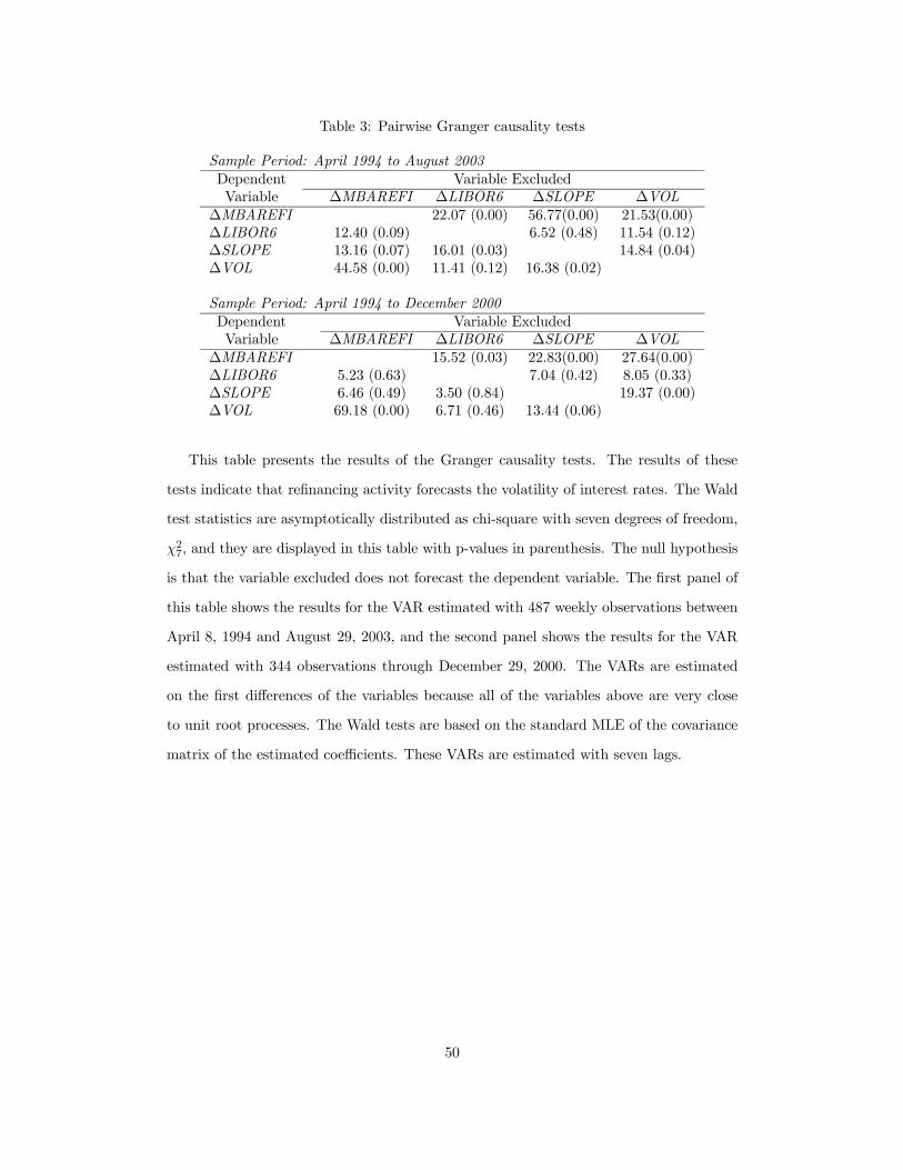
Table 3: Pairwise Granger causality tests

Sample Period: April 1994 to August 2003Dependent Variable ExcludedVariable ∆MBAREFI ∆LIBOR6 ∆SLOPE ∆VOL

∆MBAREFI 22.07 (0.00) 56.77(0.00) 21.53(0.00)∆LIBOR6 12.40 (0.09) 6.52 (0.48) 11.54 (0.12)∆SLOPE 13.16 (0.07) 16.01 (0.03) 14.84 (0.04)∆VOL 44.58 (0.00) 11.41 (0.12) 16.38 (0.02)

Sample Period: April 1994 to December 2000Dependent Variable ExcludedVariable ∆MBAREFI ∆LIBOR6 ∆SLOPE ∆VOL

∆MBAREFI 15.52 (0.03) 22.83(0.00) 27.64(0.00)∆LIBOR6 5.23 (0.63) 7.04 (0.42) 8.05 (0.33)∆SLOPE 6.46 (0.49) 3.50 (0.84) 19.37 (0.00)∆VOL 69.18 (0.00) 6.71 (0.46) 13.44 (0.06)

This table presents the results of the Granger causality tests. The results of these

tests indicate that refinancing activity forecasts the volatility of interest rates. The Wald

test statistics are asymptotically distributed as chi-square with seven degrees of freedom,

χ27, and they are displayed in this table with p-values in parenthesis. The null hypothesis

is that the variable excluded does not forecast the dependent variable. The first panel of

this table shows the results for the VAR estimated with 487 weekly observations between

April 8, 1994 and August 29, 2003, and the second panel shows the results for the VAR

estimated with 344 observations through December 29, 2000. The VARs are estimated

on the first differences of the variables because all of the variables above are very close

to unit root processes. The Wald tests are based on the standard MLE of the covariance

matrix of the estimated coefficients. These VARs are estimated with seven lags.

50

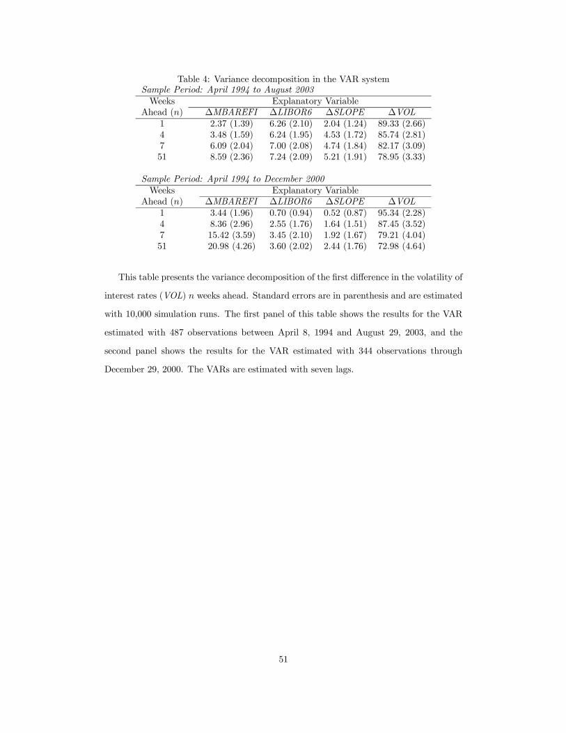
Table 4: Variance decomposition in the VAR systemSample Period: April 1994 to August 2003Weeks Explanatory Variable

Ahead (n) ∆MBAREFI ∆LIBOR6 ∆SLOPE ∆VOL1 2.37 (1.39) 6.26 (2.10) 2.04 (1.24) 89.33 (2.66)4 3.48 (1.59) 6.24 (1.95) 4.53 (1.72) 85.74 (2.81)7 6.09 (2.04) 7.00 (2.08) 4.74 (1.84) 82.17 (3.09)51 8.59 (2.36) 7.24 (2.09) 5.21 (1.91) 78.95 (3.33)

Sample Period: April 1994 to December 2000Weeks Explanatory Variable

Ahead (n) ∆MBAREFI ∆LIBOR6 ∆SLOPE ∆VOL1 3.44 (1.96) 0.70 (0.94) 0.52 (0.87) 95.34 (2.28)4 8.36 (2.96) 2.55 (1.76) 1.64 (1.51) 87.45 (3.52)7 15.42 (3.59) 3.45 (2.10) 1.92 (1.67) 79.21 (4.04)51 20.98 (4.26) 3.60 (2.02) 2.44 (1.76) 72.98 (4.64)

This table presents the variance decomposition of the first difference in the volatility of

interest rates (VOL) n weeks ahead. Standard errors are in parenthesis and are estimated

with 10,000 simulation runs. The first panel of this table shows the results for the VAR

estimated with 487 observations between April 8, 1994 and August 29, 2003, and the

second panel shows the results for the VAR estimated with 344 observations through

December 29, 2000. The VARs are estimated with seven lags.

51

Table 5: Regression of changes in mortgage rates onto changes in five-year yields

# Observations 139R2 0.90α -1.6×10−5

(-0.24)β 0.77

(34.38)

This table displays the results of the regression of the changes in mortgage rates on

the changes in the five-year zero coupon bond estimated from the Libor/swap rates; that

is, ∆MRt = α+β×∆y5−yeart . The sample is monthly from January 1992 to August 2003.

T-statistics are between parenthesis.

52

Table 6: Comparison of RMSEs of each model

Likelihood Ratio TestsH0 HA Test Statistics p-valueLSS CEVβi = 0, i = 1 to 3 βi 6= 0, i = 1 to 3 850 0.00LSS MREγi = 0, i = 1 to 3 γi 6= 0, i = 1 to 3 3,442 0.00

Diebold and Mariano TestH0 HA Test Statistics p-valueE[SSECEV ] = E[SSEMRE ] E[SSEMRE ] < E[SSECEV ] -1.85 0.03

Akaike Information CriteriaLSS -1.37MRE -2.46CEV -1.50

The first panel of this table presents the results of two likelihood ratio tests; the

second panel presents the results of one Diebold and Mariano (1995) test and the third

panel displays the Akaike information criteria for each model. The columns denoted by

H0 and HA contain the null and the alternative hypotheses respectively. The test statistic

of the two likelihood ratio tests is the difference between the log of the sum of the mean

squared-errors multiplied by the number of swaptions. These two tests have test statistic

distributed as chi-square with 240 degrees of freedom. The Diebold and Mariano test is

used because the MRE and the CEV models are non-nested. The null hypothesis of the

Diebold and Mariano test is that the MRE and CEV models have the same mean sum of

the relative squared errors (SSE). Under technical conditions, the Diebold and Mariano

test statistic is asymptotically standard normally distributed. The AIC indicates that the

MRE model is the preferred one.

53

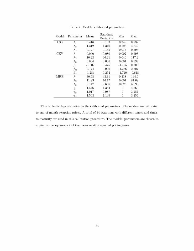
Table 7: Models’ calibrated parameters

Model Parameter MeanStandardDeviation

Min Max

LSS λ1 0.416 0.133 0.248 0.832λ2 1.312 1.310 0.128 4.842λ3 0.127 0.155 0.015 0.593

CEV λ1 0.050 0.080 0.002 0.593λ2 10.32 26.31 0.040 117.3λ3 0.004 0.006 0.001 0.039β1 -1.002 0.475 -1.755 0.305β2 0.174 0.996 -1.286 2.507β3 -1.284 0.254 -1.740 -0.618

MRE λ1 30.53 43.11 0.238 144.9λ2 11.83 16.17 0.001 87.68λ3 6.147 9.606 0.025 53.90γ1 1.546 1.364 0 4.560γ2 1.017 0.987 0 3.257γ3 1.503 1.149 0 3.459

This table displays statistics on the calibrated parameters. The models are calibrated

to end-of-month swaption prices. A total of 34 swaptions with different tenors and times-

to-maturity are used in this calibration procedure. The models’ parameters are chosen to

minimize the square-root of the mean relative squared pricing error.

54

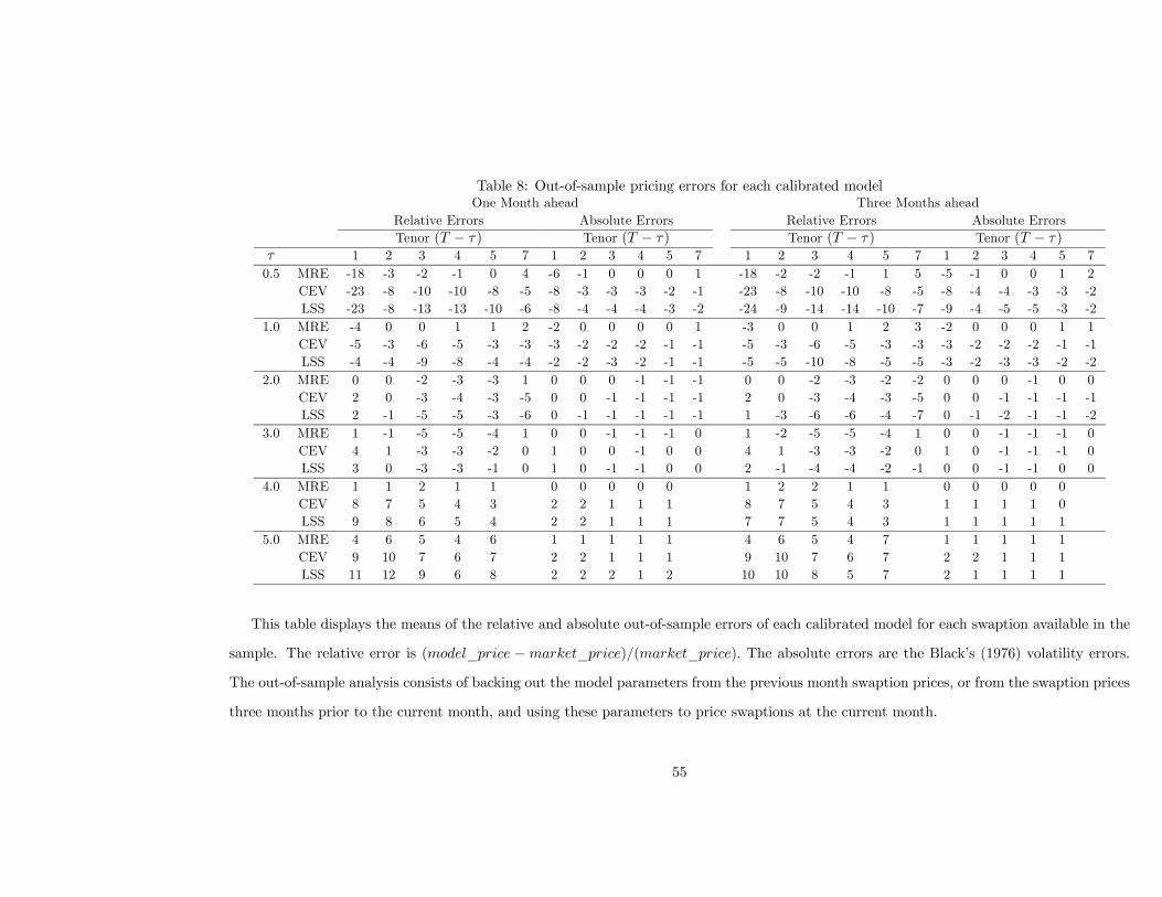
Table 8: Out-of-sample pricing errors for each calibrated modelOne Month ahead Three Months ahead

Relative Errors Absolute Errors Relative Errors Absolute ErrorsTenor (T − τ) Tenor (T − τ) Tenor (T − τ) Tenor (T − τ)

τ 1 2 3 4 5 7 1 2 3 4 5 7 1 2 3 4 5 7 1 2 3 4 5 70.5 MRE -18 -3 -2 -1 0 4 -6 -1 0 0 0 1 -18 -2 -2 -1 1 5 -5 -1 0 0 1 2

CEV -23 -8 -10 -10 -8 -5 -8 -3 -3 -3 -2 -1 -23 -8 -10 -10 -8 -5 -8 -4 -4 -3 -3 -2LSS -23 -8 -13 -13 -10 -6 -8 -4 -4 -4 -3 -2 -24 -9 -14 -14 -10 -7 -9 -4 -5 -5 -3 -2

1.0 MRE -4 0 0 1 1 2 -2 0 0 0 0 1 -3 0 0 1 2 3 -2 0 0 0 1 1CEV -5 -3 -6 -5 -3 -3 -3 -2 -2 -2 -1 -1 -5 -3 -6 -5 -3 -3 -3 -2 -2 -2 -1 -1LSS -4 -4 -9 -8 -4 -4 -2 -2 -3 -2 -1 -1 -5 -5 -10 -8 -5 -5 -3 -2 -3 -3 -2 -2

2.0 MRE 0 0 -2 -3 -3 1 0 0 0 -1 -1 -1 0 0 -2 -3 -2 -2 0 0 0 -1 0 0CEV 2 0 -3 -4 -3 -5 0 0 -1 -1 -1 -1 2 0 -3 -4 -3 -5 0 0 -1 -1 -1 -1LSS 2 -1 -5 -5 -3 -6 0 -1 -1 -1 -1 -1 1 -3 -6 -6 -4 -7 0 -1 -2 -1 -1 -2

3.0 MRE 1 -1 -5 -5 -4 1 0 0 -1 -1 -1 0 1 -2 -5 -5 -4 1 0 0 -1 -1 -1 0CEV 4 1 -3 -3 -2 0 1 0 0 -1 0 0 4 1 -3 -3 -2 0 1 0 -1 -1 -1 0LSS 3 0 -3 -3 -1 0 1 0 -1 -1 0 0 2 -1 -4 -4 -2 -1 0 0 -1 -1 0 0

4.0 MRE 1 1 2 1 1 0 0 0 0 0 1 2 2 1 1 0 0 0 0 0CEV 8 7 5 4 3 2 2 1 1 1 8 7 5 4 3 1 1 1 1 0LSS 9 8 6 5 4 2 2 1 1 1 7 7 5 4 3 1 1 1 1 1

5.0 MRE 4 6 5 4 6 1 1 1 1 1 4 6 5 4 7 1 1 1 1 1CEV 9 10 7 6 7 2 2 1 1 1 9 10 7 6 7 2 2 1 1 1LSS 11 12 9 6 8 2 2 2 1 2 10 10 8 5 7 2 1 1 1 1

This table displays the means of the relative and absolute out-of-sample errors of each calibrated model for each swaption available in the

sample. The relative error is (model_price −market_price)/(market_price). The absolute errors are the Black’s (1976) volatility errors.

The out-of-sample analysis consists of backing out the model parameters from the previous month swaption prices, or from the swaption prices

three months prior to the current month, and using these parameters to price swaptions at the current month.

55

Table 9: Forecasting interest-rate volatility

LSS CEV MRE LSS CEV MRE∆t = 1 month ∆t = 3 months

R2 6% 20% 23% 9% 26% 34%α0 9.64x10−4 -8.80x10−4 1.11x10−3 2.11x10−3 -2.62x10−4 1.84x10−3

(1.17) (-1.14) (3.01) (1.68) (-0.20) (2.74)α1 0.709 1.369 0.532 0.626 1.121 0.584

(2.23) (4.68) (4.36) (2.29) (4.05) (4.62)p-value 0.14 0.32 0.00 0.07 0.27 0.00# Obs. 79 79 79 77 77 77

∆t = 6 months ∆t = 12 monthsR2 17% 28% 36% 20% 27% 37%α0 2.19x10−3 7.06x10−4 2.54x10−3 4.05x10−3 2.55x10−3 2.76x10−3

(1.47) (0.45) (2.72) (2.39) (1.43) (2.15)α1 0.692 0.892 0.576 0.570 0.716 0.667

(3.12) (4.11) (5.27) (3.11) (3.81) (6.32)p-value 0.34 0.87 0.00 0.06 0.32 0.00# Obs. 74 74 74 68 68 68

This table displays the results of the forecasting regression σActualt+∆t = α0+α1×σImpliedt +

εt+∆t, where σActualt+∆t is the volatility of the five-year yield between t and∆t estimated from

the daily changes on the five-year discount yield and σImpliedt is the volatility of the five-

year yield between t and t+∆t implied by a swaption pricing model at time t. Standard

errors are corrected for autocorrelation on the residuals with the Newey and West (1987)

estimator. The p-values are for the Wald test with the null hypothesis that α0 = 0 and

α1 = 1. T-statistics are in parentheses. The T-statistics are for the null hypothesis that

αi = 0, i = 0, 1. The results indicate that the MRE model outperforms the benchmarks

in forecasting future interest rate volatility. The MRE forecasts are, however, biased in

the sense that the null hypothesis that α0 = 0 and α1 = 1 is rejected in all regressions

with implied volatilities generated by the MRE model.

56

Figure 1. MBA Refinancing Index and interest rate volatility. This figure displays the Mortgage BankersAssociation (MBA) Refinancing Index and the average Black's (1976) volatility of the swaptions with threemonths to maturity (VOL ). The index is based on the number of applications for mortgage refinancing. Theindex is calculated every week and is based on the weekly survey of the MBA. The index is seasonally adjusted.This figure shows a series of spikes in refinancing activity. These spikes are refinancing waves caused by a dropin the mortgage rate to levels substantially below the current average coupon of the mortgage universe. Thespikes in mortgage refinancing are generally accompanied by spikes in interest rate volatility.

0%5%

10%15%20%25%30%35%40%45%50%55%60%65%70%

Apr

-94

Aug

-94

Dec

-94

Apr

-95

Aug

-95

Dec

-95

Apr

-96

Aug

-96

Dec

-96

Apr

-97

Aug

-97

Dec

-97

Apr

-98

Aug

-98

Dec

-98

Apr

-99

Aug

-99

Dec

-99

Apr

-00

Aug

-00

Dec

-00

Apr

-01

Aug

-01

Dec

-01

Apr

-02

Aug

-02

Dec

-02

Apr

-03

Aug

-03

Inte

rest

rate

vol

atili

ty (V

OL )

0

2000

4000

6000

8000

10000

12000

Inde

x va

lue

VOL

MBA Refinancing Index

Figure 2. MBA Refinancing Index and prepayment speed of the mortgage universe. The top panel displaysthe time series of the proxy of the actual CPR of the mortgage universe, the CPR estimated with the prepaymentmodel described in Section 4.2.1, and the monthly average of the MBA Refinancing Index. Note that these seriestrend together and that the MBA Refinancing Index anticipates the CPR in the mortgage universe. This isunsurprising because there is a delay between the application for refinancing and the actual prepayment of amortgage. The bottom panel displays the average prepayment speed of the MBS universe as function ofrefinancing incentive. The refinancing incentive is defined as the proxy of the weighted-average coupon (WAC)of the mortgage universe divided by the proxy of the mortgage rate. The prepayment model is non-parametricallyestimated with data between January 1997 and August 2003. Each dot in the bottom panel represents oneobservation.

5%10%15%20%25%30%35%40%45%50%55%60%65%70%

Jan-

97

May

-97

Sep-

97

Jan-

98

May

-98

Sep-

98

Jan-

99

May

-99

Sep-

99

Jan-

00

May

-00

Sep-

00

Jan-

01

May

-01

Sep-

01

Jan-

02

May

-02

Sep-

02

Jan-

03

May

-03

Sep-

03

Prep

aym

ent s

peed

(CPR

)

0

1000

2000

3000

4000

5000

6000

7000

8000

9000

10000

Inde

x va

lue

Actual prepayment

Model prepayment

Montlhy average MBA Refinancing Index

0%

10%

20%

30%

40%

50%

60%

70%

0.4 0.6 0.8 1 1.2 1.4 1.6WAC/Current mortgage rate

CPR

Figure 3. Impulse response functions. This figure shows the cumulative impulse response functions of VOL and MBAREFI in the estimated VAR. The VAR is estimated on the first differences of four variables: themortgage refinancing activity (MBAREFI ), the six-month Libor (LIBOR6 ), the difference between the five-year discount yield and the six-month LIBOR (SLOPE ), and the average implied volatility of short-termswaptions (VOL ). The left panels display the response on the variable VOL to a shock in each variable. Theright panels display the response on the variable MBAREFI to a shock in each variable. The shock in eachvariable is equal to one standard deviation in its orthogonalized innovation. The dashed lines represent twostandard deviations estimated by 10,000 Monte Carlo runs.

Response of VOL to MBAREFI

-0.005

0

0.005

0.011 6 11 16 21 26 31 36 41 46 51

Weeks

Response of VOL to LIBOR6

-0.015-0.01

-0.0050

0.005

1 6 11 16 21 26 31 36 41 46 51

Weeks

Response of VOL to SLOPE

-0.01

-0.005

0

0.005

1 6 11 16 21 26 31 36 41 46 51

Weeks

Response of VOL to VOL

00.005

0.010.015

0.02

1 6 11 16 21 26 31 36 41 46 51

Weeks

Response of MBAREFI to MBAREFI

0

0.02

0.04

0.06

1 6 11 16 21 26 31 36 41 46 51

Weeks

Response of MBAREFI to LIBOR6

-0.03-0.02-0.01

00.01

1 6 11 16 21 26 31 36 41 46 51

Weeks

Response of MBAREFI to SLOPE

-0.04-0.03-0.02-0.01

0

1 6 11 16 21 26 31 36 41 46 51

Weeks

Response of MBAREFI to VOL

0

0.01

0.02

0.03

1 6 11 16 21 26 31 36 41 46 51

Weeks

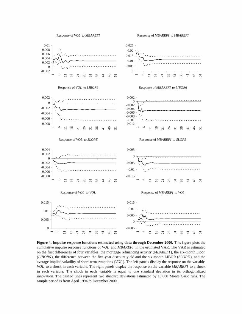
Figure 4. Impulse response functions estimated using data through December 2000. This figure plots thecumulative impulse response functions of VOL and MBAREFI in the estimated VAR. The VAR is estimatedon the first differences of four variables: the mortgage refinancing activity (MBAREFI ), the six-month Libor(LIBOR6 ), the difference between the five-year discount yield and the six-month LIBOR (SLOPE ), and theaverage implied volatility of short-term swaptions (VOL ). The left panels display the response on the variableVOL to a shock in each variable. The right panels display the response on the variable MBAREFI to a shockin each variable. The shock in each variable is equal to one standard deviation in its orthogonalizedinnovation. The dashed lines represent two standard deviations estimated by 10,000 Monte Carlo runs. Thesample period is from April 1994 to December 2000.

Response of VOL to MBAREFI

-0.0020

0.0020.0040.0060.0080.01

1 6 11 16 21 26 31 36 41 46 51

Response of VOL to LIBOR6

-0.008-0.006-0.004-0.002

00.002

1 6 11 16 21 26 31 36 41 46 51

Response of VOL to SLOPE

-0.008-0.006-0.004-0.002

00.0020.004

1 6 11 16 21 26 31 36 41 46 51

Response of VOL to VOL

0

0.005

0.01

0.015

1 6 11 16 21 26 31 36 41 46 51

Response of MBAREFI to MBAREFI

00.005

0.010.015

0.020.025

1 6 11 16 21 26 31 36 41 46 51

Response of MBAREFI to LIBOR6

-0.012-0.01

-0.008-0.006-0.004-0.002

00.002

1 6 11 16 21 26 31 36 41 46 51

Response of MBAREFI to SLOPE

-0.015

-0.01

-0.005

0

0.005

1 6 11 16 21 26 31 36 41 46 51

Response of MBAREFI to VOL

-0.005

0

0.005

0.01

0.015

1 6 11 16 21 26 31 36 41 46 51

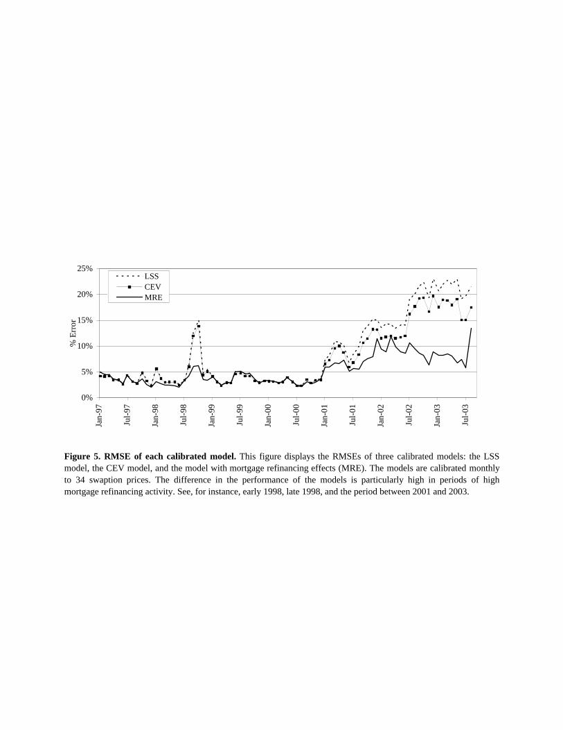
Figure 5. RMSE of each calibrated model. This figure displays the RMSEs of three calibrated models: the LSSmodel, the CEV model, and the model with mortgage refinancing effects (MRE). The models are calibrated monthlyto 34 swaption prices. The difference in the performance of the models is particularly high in periods of highmortgage refinancing activity. See, for instance, early 1998, late 1998, and the period between 2001 and 2003.

0%

5%

10%

15%

20%

25%

Jan-

97

Jul-9

7

Jan-

98

Jul-9

8

Jan-

99

Jul-9

9

Jan-

00

Jul-0

0

Jan-

01

Jul-0

1

Jan-

02

Jul-0

2

Jan-

03

Jul-0

3

% E

rror

LSSCEVMRE

Figure 6. The term structure of swaption volatilities. Panels A, B, and C of this figure present theaverage of the Black's (1976) volatility of swaptions by time-to-maturity in periods when the refinancingactivity is high and the models without refinancing effects have a RMSE greater than 5%. Panel Dpresents the term structure of swaption volatilities in the other periods. The lines denoted by "Real" arethe Black's volatility of the actual swaption prices. The other lines are the Black's volatilities of theswaption prices calculated by each model. The term structure of swaption volatilities is downward-sloped in periods of high refinancing and practically flat in periods of low refinancing activity. TheMRE model adapts well to the change in the term structure of swaption volatilities.

C - Average implied volatility between January 2001 and August 2003

13%

18%

23%

28%

33%

0 0.5 1 1.5 2 2.5 3 3.5 4 4.5 5Years to swaption maturity

Real MRECEV LSS

D - Average implied volatility in periods of low refinancing activity

13%

14%

15%

16%

17%

18%

0 0.5 1 1.5 2 2.5 3 3.5 4 4.5 5Years to swaption maturity

Real MRECEV LSS

B - Average implied volatility between August 1998 and October 1998

13%

15%

17%

19%

21%

0 0.5 1 1.5 2 2.5 3 3.5 4 4.5 5Years to swaption maturity

Real MRECEV LSS

A - Average implied volatility in January 1998

13%

14%

15%

16%

17%

18%

0 0.5 1 1.5 2 2.5 3 3.5 4 4.5 5Years to swaption maturity

Real MRECEV LSS