CHAPTER 4

The Cahn–Hilliard Equation

Amy Novick-CohenTechnion-IIT, Haifa 32000, Israel

Contents1. Introduction . . . . . . . . . . . . . . . . . . . . . . . . . . . . . . . . . . . . . . . . . . . . . . . . . . . 2032. Backwards diffusion and regularization . . . . . . . . . . . . . . . . . . . . . . . . . . . . . . . . . . . . 2043. The Cahn–Hilliard equation and phase separation . . . . . . . . . . . . . . . . . . . . . . . . . . . . . . 2064. Two prototype formulations . . . . . . . . . . . . . . . . . . . . . . . . . . . . . . . . . . . . . . . . . . 208

4.1. The constant mobility – quartic polynomial case . . . . . . . . . . . . . . . . . . . . . . . . . . . . 2084.2. The degenerate mobility – logarithmic free energy case . . . . . . . . . . . . . . . . . . . . . . . . 209

5. Existence, uniqueness, and regularity . . . . . . . . . . . . . . . . . . . . . . . . . . . . . . . . . . . . . 2116. Linear stability and spinodal decomposition . . . . . . . . . . . . . . . . . . . . . . . . . . . . . . . . . 2147. Comparison with experiment . . . . . . . . . . . . . . . . . . . . . . . . . . . . . . . . . . . . . . . . . 2168. Long time behavior and limiting motions . . . . . . . . . . . . . . . . . . . . . . . . . . . . . . . . . . . 216

8.1. The Mullins–Sekerka problem . . . . . . . . . . . . . . . . . . . . . . . . . . . . . . . . . . . . . . 2178.2. Surface diffusion . . . . . . . . . . . . . . . . . . . . . . . . . . . . . . . . . . . . . . . . . . . . . 219

9. Upper bounds for coarsening . . . . . . . . . . . . . . . . . . . . . . . . . . . . . . . . . . . . . . . . . . 219Acknowledgements . . . . . . . . . . . . . . . . . . . . . . . . . . . . . . . . . . . . . . . . . . . . . . . . 225References . . . . . . . . . . . . . . . . . . . . . . . . . . . . . . . . . . . . . . . . . . . . . . . . . . . . . 225

HANDBOOK OF DIFFERENTIAL EQUATIONSEvolutionary Equations, Volume 4Edited by C.M. Dafermos and E. Feireisl© 2008 Elsevier B.V. All rights reservedDOI: 10.1016/S1874-5717(08)00004-2

201

The Cahn–Hilliard equation 203

1. Introduction

The present chapter is devoted to the Cahn–Hilliard equation [16,15]:

(1)ut = ∇ · M(u)∇[f (u) − ε2�u

], (x, t) ∈ Ω × R

+,

(2)n · ∇u = n · M(u)∇[f (u) − ε2�u

] = 0, (x, t) ∈ ∂Ω × R+,

(3)u(x, 0) = u0(x), x ∈ Ω.

Here 0 < ε2 � 1 is a “coefficient of gradient energy”, M = M(u) is a “mobility” coeffi-cient, and f = f (u) is a “homogeneous free energy”. The equation was initially developedto describe phase separation is a two component system, with u = u(x, t) representing theconcentration of one of the two components. Typically, the domain Ω is assumed to be abounded domain with a “sufficiently smooth” boundary, ∂Ω , with n in (2) representing theunit exterior normal to ∂Ω . It is reasonable to consider evolution for times t > 0, or onsome finite time interval 0 < t < T < ∞.

Concentration should be understood as referring either to volume fraction or to massfraction, depending on the physical system under investigation. By volume fraction wemean the volume fraction per unit volume of say component “A”, in a system containingtwo components which we shall denote by “A” and “B”. The meaning of mass fractionis analogous. Thus the Cahn–Hilliard equation constitutes a continuous, as opposed to adiscrete or lattice description, of the material undergoing phase separation. Such a descrip-tion is appropriate under many but not all circumstances. Note that the definition of u(x, t)

implies that u(x, t) should satisfy 0 � u(x, t) � 1. Moreover, if u(x, t), the concentrationof component A, is known, then the concentration of the second component is given by1−u and is hence also known; thus the evolution of the composition of the two componentsystem is being predicted by a single scalar Cahn–Hilliard equation.

In the context of the Cahn–Hilliard equation, the two components could refer, for ex-ample, to a system with two metallic components, or two polymer components, or say,two glassy components. Frequently in materials science literature, concentration is givenin terms of mole fraction or equivalently number fraction, rather than in terms of volumefraction or mass fraction. A mole refers to 6.02252 × 1023 molecules (Avogadro’s numberof molecules), and the mole fraction of component A refers to the number of A moleculesper mole of the two component system, locally evaluated. Mole fraction of number frac-tion are equivalent to volume fraction if the molar volume (the volume occupied by onemole) is independent of composition, which is rarely strictly correct [15]. For example, ina two component polymer systems when many of the polymers are long, the configurationof the polymers, i.e. whether they are “stretched out” or “rolled up”, typically depends oncomposition, which in turn influences the molar volume. Notice also that often temperaturedoes not appear explicitly in the Cahn–Hilliard equation, since the model is based on theassumption that the temperature is constant; such an assumption requires careful tempera-ture control and is also rarely strictly fulfilled in reality. The model also assumes isotropyof the system, which can also only be approximately correct for metallic systems [5,77,87], for which the equations were designed, which have an inherent crystalline structureunless they are in a liquid phase. Nevertheless, the Cahn–Hilliard equation has been seen tocontain many of the dominant paradigms for phase separation dynamics, and as such, has

204 A. Novick-Cohen

played, and continues to play, an important role in understanding the evolution of phaseseparation.

Why does the Cahn–Hilliard equation appear in so many different contexts, and what be-havior is predicted by the Cahn–Hilliard equation which is common to all these systems?Off-hand, what is being modeled with the Cahn–Hilliard equation is phase separation, inother words, the segregation of the system into spatial domains predominated by one ofthe components, in the presence of a mass constraint, and what one wishes to accomplishhere is to model the dynamics in a sufficiently accurate fashion so that many of the variousfeatures of the resultant pattern formation evolution that one sees in nature during phaseseparation can be explained and predicted. In materials science this pattern formation isreferred to as the microstructure of the material, and the microstructure is highly influen-tial in determining many of the properties of the material, such as strength, hardness, andconductivity. The Cahn–Hilliard model is rather broad ranged in its evolutionary scope; itcan serve as a good model for many systems during early times, it can give a reasonablequalitative description for these systems during intermediary times, and it can serve as agood model for even more systems at late times. Often, the late time evolution is so slowthat the pattern formation or microstructure becomes effectively frozen into the systemover time scales of interest, and hence it is the long time behavior of the system which isseen in practice.

The Cahn–Hilliard equation also appears in modeling many other phenomena. Theseinclude the evolution of two components of intergalactic material [80], the dynamics oftwo populations [19], the biomathematical modeling of a bacterial film [46], and certainthin film problems [69,79]. We apologies to the reader that most of the details pertaining tothe modeling of these phenomena are outside the scope of the present survey. Nevertheless,we invite the interested reader to have a look at the forthcoming book by the author ofthis survey, entitled From Backwards Diffusion to Surface Diffusion: the Cahn–HilliardEquation [65], where these and other details will be treated in greater depth.

We hope that this survey will clarify for the reader the notions of backwards diffusionand surface diffusion and their connection with the Cahn–Hilliard equation, and will con-vey something of the nature of the physical phenomena which accompany phase separationand how the Cahn–Hilliard equation manages to capture these features.

2. Backwards diffusion and regularization

Let us consider a simple variant of the Cahn–Hilliard equation in which f (u) = −u + u3

and M(u) = M0, where M0 > 0 is constant. Let t ∈ (0, T ), 0 < T < ∞, and Ω = (0, L).In most applications, Ω ∈ R

n with n = 2 or n = 3 is most physically relevant. However,let us focus temporarily on the n = 1 case for simplicity. Thus,

(4)

⎧⎪⎨

⎪⎩

ut = M0[−u + u3 − ε2uxx

]xx

, (x, t) ∈ ΩT ,

ux = M0[−u + u3 − ε2uxx

]x

= 0, (x, t) ∈ ∂ΩT ,

u(x, 0) = u0(x), x ∈ Ω,

The Cahn–Hilliard equation 205

where ΩT = (0, T ) × Ω and ∂ΩT = {0, L} × (0, T ). Note that u(x, t) = u constitutesa steady state of (4), where u is an arbitrary constant; however if u(x, t) is to representconcentration, clearly one must assume that 0 � u � 1.

Let us now suppose that u0(x) = u+ u0(x), where u0(x) represents a small perturbationfrom spatial uniformity. Setting u(x, t) = u + u(x, t), (4) yields that

(5)

⎧⎪⎨

⎪⎩

ut = M0[−u + [u + u]3 − ε2uxx

]xx

, (x, t) ∈ ΩT ,

ux = M0[−u + [u + u]3 − ε2uxx

]x

= 0, (x, t) ∈ ∂ΩT ,

u(x, 0) = u0(x) := u0(x) − u, x ∈ Ω.

Assuming (5) to be well-posed and u(x, t) to be small, we neglect terms which are nonlin-ear in u(x, t) and obtain to leading order the linearized problem

(6)

⎧⎪⎨

⎪⎩

ut = M0[−(

1 − 3u2)u − ε2uxx

]xx

, (x, t) ∈ ΩT ,

ux = M0[−(

1 − 3u2)u − ε2uxx

]x

= 0, (x, t) ∈ ∂ΩT ,

u(x, 0) = u0(x), x ∈ Ω.

We recall that we have assumed earlier that 0 < ε2 � 1. Suppose that we optimisticallyneglect terms in the system (6) which contain a factor of ε2. This yields

(7)

⎧⎪⎨

⎪⎩

ut = −M0(1 − 3u2)uxx, (x, t) ∈ ΩT ,

ux = −M0(1 − 3u2)ux = 0, (x, t) ∈ ∂ΩT ,

u(x, 0) = u0(x), x ∈ Ω.

If we stop and consider for a moment (7), we can see that for 3u2−1 > 0, it is equivalentto the classical diffusion equation with Neumann boundary conditions

(8)

⎧⎨

⎩

ut = Duxx, (x, t) ∈ ΩT ,

ux = 0, (x, t) ∈ ∂ΩT ,

u(x, 0) = u0(x), x ∈ Ω,

whose solutions decay to 1L

∫ L

0 u0(x) dx. For 3u2 − 1 > 0, it is equivalent to

(9)

⎧⎨

⎩

ut = −Duxx, (x, t) ∈ ΩT ,

ux = 0, (x, t) ∈ ∂ΩT ,

u(x, 0) = u0(x), x ∈ Ω.

Now (9) is precisely the backwards diffusion equation, which can be obtained from theclassical diffusion equation by redefining time t → −t so that time will “run backwards.”The problem (9) is notoriously ill-posed as can be verified by noting that for u0 ∈ L2(Ω),it possesses the formal separation of variables solution

(10)u(x, t) = A0

2+

∞∑

n=1

Anen2π2

L2 tcos(nπx/L),

where the coefficients Ai , i = 0, 1, 2, . . . , correspond to the Fourier coefficients of theinitial conditions,

(11)u(x, 0) = u0(x) = A0

2+

∞∑

n=1

An cos(nπx/L).

206 A. Novick-Cohen

Its amplitude grows without bound

(12)∥∥u(x, t)

∥∥2L2[0,L] = A2

0

2+

∞∑

n=1

A2ne

2n2π2

L2 t ;

even for initial data based on a single mode, u0(x) = Ak cos(kπx/L),

(13)∥∥u(x, t)

∥∥2L2[0,L] = A2

ke2k2π2

L2 t.

This clearly makes little physical sense in terms of a model for phase separation, althoughin other contexts, such as image processing [17], it has been successfully implemented. Inparticular, we see that the solution, u(x, t) = u + u(x, t) does not remain bounded withinthe interval [0, 1] over time.

Thus both problems, (8) and (9), make little physical sense as models for phase separa-tion. Hence, the higher order terms proportional to ε2 are truly necessary in the physicalmodel, and cannot be made light of easily. Seemingly this would provide a compelling rea-son to include such regularizing terms, but in fact regularizing terms were already addedmuch before the dynamics for phase separation came under consideration, when equilib-rium considerations lead to the search for a free energy with “phase separated” steady statespossessing certain regularity and uniqueness properties. This reflects the independent sci-entific contribution of Gibbs (1893) [35] and van der Waals (1973) [81].

The reader should have no difficulty in ascertaining that (6), where the regularizing termshave been included, can be formulated as a well-posed problem, and it is fairly straightfor-ward to verify that (5) and (4) can be carefully formulated as well-posed problems as well.However, before discussing existence, uniqueness, and well-posedness, we first briefly con-sider what are the physical phenomena one should like to model with the Cahn–Hilliardequation, and which are the most important variants of the Cahn–Hilliard equation whichone should like to consider.

3. The Cahn–Hilliard equation and phase separation

We now outline what are the physical features and phenomena which one should like tobe described by the Cahn–Hilliard equation. The process of phase separation in two com-ponent systems is accompanied by pattern formation and evolution. A typical scenario weshould like to model is that of quick quenching. Let Ω ⊂ R

3 initially contain two compo-nents which are roughly uniformly distributed, so that u(x, 0) ≈ u0(x) ≡ u. We shouldsuppose that u ∈ [0, 1] if u(x, t) is to represent concentration. If there is no flux of materialinto or out of Ω , then the total amount of each component should be conserved,

(14)1

|Ω|∫

Ω

u(x, t) dx = u, 0 � t � T .

Let the initial temperature be given by Θ0, and let the temperature of the system be nowrapidly lowered (quick quenched) to some new temperature, Θ1 � Θ0. In two componentmetallic alloy systems, the average thermal conductivity is high, and the temperature of thesystem will equilibrate rapidly to the new temperature. With this in mind, the assumption

The Cahn–Hilliard equation 207

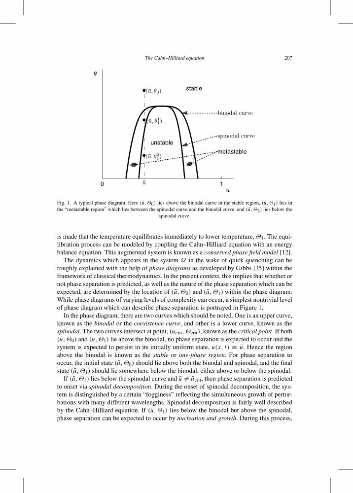
Fig. 1. A typical phase diagram. Here (u,Θ0) lies above the binodal curve in the stable region, (u,Θ1) lies inthe “metastable region” which lies between the spinodal curve and the binodal curve, and (u,Θ2) lies below the

spinodal curve.

is made that the temperature equilibrates immediately to lower temperature, Θ1. The equi-libration process can be modeled by coupling the Cahn–Hilliard equation with an energybalance equation. This augmented system is known as a conserved phase field model [12].

The dynamics which appears in the system Ω in the wake of quick quenching can beroughly explained with the help of phase diagrams as developed by Gibbs [35] within theframework of classical thermodynamics. In the present context, this implies that whether ornot phase separation is predicted, as well as the nature of the phase separation which can beexpected, are determined by the location of (u,Θ0) and (u,Θ1) within the phase diagram.While phase diagrams of varying levels of complexity can occur, a simplest nontrivial levelof phase diagram which can describe phase separation is portrayed in Figure 1.

In the phase diagram, there are two curves which should be noted. One is an upper curve,known as the binodal or the coexistence curve, and other is a lower curve, known as thespinodal. The two curves intersect at point, (ucrit,Θcrit), known as the critical point. If both(u,Θ0) and (u,Θ1) lie above the binodal, no phase separation is expected to occur and thesystem is expected to persist in its initially uniform state, u(x, t) ≡ u. Hence the regionabove the binodal is known as the stable or one-phase region. For phase separation tooccur, the initial state (u,Θ0) should lie above both the binodal and spinodal, and the finalstate (u,Θ1) should lie somewhere below the binodal, either above or below the spinodal.

If (u,Θ1) lies below the spinodal curve and u = ucrit, then phase separation is predictedto onset via spinodal decomposition. During the onset of spinodal decomposition, the sys-tem is distinguished by a certain “fogginess” reflecting the simultaneous growth of pertur-bations with many different wavelengths. Spinodal decomposition is fairly well describedby the Cahn–Hilliard equation. If (u,Θ1) lies below the binodal but above the spinodal,phase separation can be expected to occur by nucleation and growth. During this process,

208 A. Novick-Cohen

phase separation occurs via the appearance or nucleation of localized perturbations in theuniform state u which persist and grow if they are sufficiently large. Though we mentionthe nucleation and growth process, it is not well modeled by the Cahn–Hilliard equation,and alternative approaches have been developed for purpose such as the Lifshitz–Slyozovtheory of Oswald ripening [49] and its extensions [42,4].

We caution the reader that if (u,Θ0) or (u,Θ1) are too close to (ucrit,Θcrit), then theabove descriptions are inappropriate, since critical phenomena [23], such as critical slow-ing down, will accompany the phase separation. Such effects are characteristic of secondorder phase transitions, as opposed to our earlier description, which was appropriate forfirst order phase transitions. Arguably Θ1 should be taken not too far from Θcrit, other-wise inertial and higher order effects may become important; these effects would renderthe Cahn–Hilliard model inaccurate, and make it difficult to control the phase separationprocess and the resultant microstructure. What distinguishes a first order phase transitionfrom a second or higher order phase transition is the degree of continuity or regularity ofthe system as the system crosses from the stable regime above the binodal into the unstableregime which lies below it, see e.g. [50].

Whether phase separation occurs via spinodal decomposition or via nucleation andgrowth, eventually the system saturates into well-defined spatial domains in which oneof the two components dominates, so that u ≈ uA or by u ≈ uB , where uA and uB denotethe binodal or limiting miscibility gap concentrations when Θ = Θ1. See Figure 1. Theaverage size of these spatial domains increases over time, as larger domains grow at theexpense of smaller domains. This process is called coarsening, and the dynamics of thesystem may now be characterized by the motion of the boundaries or interfaces betweenthese various domains. Because of mass balance, (14), the relative volume or area of thedomains where u ≈ uA and u ≈ uB remains unchanged, but the overall amount of “do-main interface” decreases as some limiting configuration is seemingly approached. Whilenucleation and growth is somewhat of a weak spot for the Cahn–Hilliard theory, the Cahn–Hilliard equation can give some reasonable description of the coarsening process, even ifthe initial stages of the phase separations were dominated by nucleation and growth.

Let us now consider two important cases of the Cahn–Hilliard equation formulationgiven in (1)–(3), to which we shall refer to later repeatedly.

4. Two prototype formulations

Perhaps the easiest formulation to consider is that given in (4) which was discussed inSection 2. We shall refer to this case as the constant mobility-quartic polynomial case, ormore briefly, the constant mobility Cahn–Hilliard equation, and it is summarized below.

4.1. The constant mobility – quartic polynomial case

Let

(15)M(u) = M0 > 0, where M0 is a constant, and f (u) = −u + u3.

The Cahn–Hilliard equation 209

It follows from (15) that

(16)f (u) = F ′(u), F (u) = 1

4

(u2 − 1

)2.

Within this framework, the Cahn–Hilliard equation is given by

(17)

{ut = M0�(−u + u3 − ε2�u), (x, t) ∈ Ω × (0, T ),

n · ∇u = n · ∇�u = 0, (x, t) ∈ ∂Ω × (0, T ),

in conjunction with appropriate initial conditions. The value of M0 may be set to unity byrescaling time, but we maintain M0 in the formulation since it is frequently maintained inthe literature, [62]. Note that (17) is invariant under the transformation u → −u, because u

in (17) represents the difference between the two concentrations, u ≡ uA −uB = 2uA −1.Thus, in terms of the physical interpretation, u(x, t) should assume values in the interval[−1, 1].

The analysis and treatment of this case is relatively easy since (17) constitutes a fourthorder semilinear parabolic equation, whose treatment is similar to that of second semilinearparabolic equations such as the reaction diffusion equation,

(18)ut = ε2�u − f (u),

which arises in a wide variety of applications, from populations genetics to tiger spots,[56,57]. Nevertheless, one of the mainstays in the treatment of second order equations, themaximum principle, does not carry over easily into the fourth order setting [53]. An exis-tence theory can be given, for example, in terms of Galerkin approximations [78] whichcan also be used to construct finite element approximations that can be implemented nu-merically. From numerical calculations and analytical consideration, it can be seen thatfor a sensible choice of initial conditions, (17) gives a reasonable description of spinodaldecomposition and of coarsening.

An unfortunate feature of the constant mobility Cahn–Hilliard variant (17) is that itssolutions need not remain bounded between −1 and 1, even if the initial data lies in this in-terval. This drawback can be avoided by employing a formulation, written in terms of oneof the concentrations, in which the mobility is taken to degenerate when u = 0 and u = 1,and the free energy is taken to be well behaved, as was demonstrated in one space dimen-sion by Jingxue [44]. Such a formulation does not occur so naturally in the context of phaseseparation, but is does occur naturally in other contexts, such as in structure formation inbiofilms [46]. In the context of phase separation, it is natural in including a degeneratemobility to also include logarithmic terms in the free energy. This seemingly less naturalformulation is in fact well-based in terms of the physics; the logarithmic terms reflectentropy contributions and the vanishing of the mobilities reflects jump probability consid-erations [72]. We shall refer to this formulation as the degenerate mobility-logarithmic freeenergy case, or for short, the degenerate Cahn–Hilliard equation, and it is explained below.

4.2. The degenerate mobility – logarithmic free energy case

Here we assume that

(19)M(u) = u(1 − u) and f (u) = F ′(u),

210 A. Novick-Cohen

where

(20)F(u) = Θ

2

{u ln u + (1 − u) ln(1 − u)

} + αu(1 − u),

with Θ > 0, α > 0. In (20), Θ denotes temperature, or more accurately a scaled tempera-ture. The resultant Cahn–Hilliard formulation is now:

(21)

⎧⎪⎪⎪⎪⎨

⎪⎪⎪⎪⎩

ut = ∇ · M(u)∇{

Θ

2ln

[u

1 − u

]+ α(1 − 2u) − ε2�u

}, (x, t) ∈ ΩT ,

n · ∇u = 0, (x, t) ∈ ∂ΩT ,

n · M(u)

{Θ

2u(1 − u)∇u − 2α∇u − ε2∇�u

}= 0, (x, t) ∈ ∂ΩT ,

where ΩT = Ω × (0, T ) and ∂ΩT = ∂Ω × (0, T ), and the equation and boundaryconditions are to be solved in conjunction with appropriate initial data, u0(x). Since u(x, t)

represents here the concentration of one of the two components, u0(x) and u(x, t) shouldsatisfy 0 � u0(x), u(x, t) � 1.

Formally, referring to (19), (21) can be written more simply as

(22)

⎧⎨

⎩ut = Θ

2�u − ∇ · M(u)∇{

2αu + ε2�u}, (x, t) ∈ ΩT ,

n · ∇u = n · M(u)∇�u = 0, (x, t) ∈ ∂ΩT .

Note though that (22) is in fact only meaningful for u ∈ [0, 1], and M(u) has only beendefined on that interval.

The mobility in (19) is referred to as a degenerate mobility, since it is not strictly pos-itive. A concentration dependent mobility was already considered by Cahn in 1961 [15],and a degenerate mobility similar to (19) appeared in the work by Hillert in 1956 [40,39] ona one-dimensional discretely defined precursor of the Cahn–Hilliard equation. The use oflogarithmic terms in the free energy, which arises naturally due to thermodynamic entropyconsideration, also appeared in the papers [40,39] as well as in the 1958 paper of Cahnand Hilliard [16]. See also the discussions in [26,41]. The problem formulated in (21) con-stitutes a degenerate fourth order semilinear parabolic problem. Galerkin approximationscan be used to prove existence and to construct finite element schemes by first regularizingthe free energy. The payoff for working with the more complicated formulation is that ityields more physical results; namely, for (21) and for Ω ⊂ R

n, n ∈ N, if u0 ∈ [0, 1], thenu(x, t) ∈ [0, 1] for t � 0. Details follow in the next section.

However, early on the degenerate and concentration dependent mobilities were replacedby constant mobilities and logarithmic terms in the free energy were expanded into polyno-mials, to simplify the analysis and to enable some qualitative understanding of the equation.In fact, very early analyzes were totally linear. Surprisingly this was not such a bad pathto take since the dominant unstable modes are typically sustained longer that a straightforward linear analysis would suggest, see Section 6. It seems that nonlinear effects werefirst included by de Fontaine in 1967 [22], who did so in the context of early numericalstudies of the Cahn–Hilliard equation.

For detailed derivations of both variants, see [65,66,34]. Physically speaking, it is morenatural to first justify the degenerate Cahn–Hilliard equation with logarithmic free energy

The Cahn–Hilliard equation 211

terms and then to obtain the constant mobility Cahn–Hilliard equation with a polynomialfree energy by making suitable approximations.

5. Existence, uniqueness, and regularity

For the constant mobility Cahn–Hilliard equation with a polynomial free energy, a proofof existence and uniqueness was given in 1986 by Elliott and Songmu [27], which alsocontains a finite element Galerkin approximation scheme. To be more precise, setting

H 2E(Ω) = {

v ∈ H 2(Ω) | n · ∇v = 0 on ∂Ω},

where n denotes the unit exterior normal to ∂Ω , and ΩT = Ω × (0, T ), it follows from[27] that

THEOREM 5.1. If Ω is a bounded domain in Rn, n � 2, with a smooth boundary, then

for any initial data u0 ∈ H 2E(Ω) and T > 0, there exists a unique global solution in

H 4,1(ΩT ).

The proof relies on Picard iteration and on a priori estimates obtained by multiply-ing (17) by u, f (u)−ε2�u, and �2u. By taking more regular initial data, classical solutionsmay also be obtained. Of some physical interest is the estimate obtained by multiplying(17) by f (u) − ε2�u, namely

(23)F(t) − F(0) = −∫

ΩT

∣∣∇{f (u) − ε�u

}∣∣2 dx dt,

where

(24)F(t) =∫

Ω

{F(u) + ε2

2|∇u|2

}dx.

The quantity f (u) − ε2�u is frequently identified as the chemical potential, μ = μ(x, t).Of interest also is the estimate obtained by multiplying (17) by φ ≡ 1, namely

(25)∫

Ω

u(x, t) dx =∫

Ω

u0(x) dx,

which can be understood as a statement of conservation of mass or conservation of themean.

From (23), (25), it also follows that

F(t) − F(0) =∫

ΩT

⟨f (u) − ε2�u, ut

⟩H 1(Ω),(H 1(Ω))′ dt

(26)= −‖ut‖2L2(0,T ;H−1(Ω))

,

and hence the Cahn–Hilliard equation is frequently referred to as H−1 gradient flow.In [58] (see [78] for an extended explanation), using essentially the same estimates and

a Galerkin approximation based on the eigenfunctions of A, where A is the Laplacian withNeumann boundary conditions, it is proven that

212 A. Novick-Cohen

THEOREM 5.2. For u0(x) ∈ L2(Ω), Ω ⊂ Rn, n � 3, there exists a unique solution,

u(x, t), to the constant mobility Cahn–Hilliard equation, and u(x, t) satisfies

(27)

u ∈ C([0, T ]; L2(Ω)

) ∩ L2(0, T ; H 1(Ω)) ∩ L4(0, T ; L4(Ω)

), ∀T > 0,

and F(t) decays along orbits. If, moreover, u0(x) ∈ H 2E(Ω), then

(28)u ∈ C([0, T ]; H 2

E(Ω)) ∩ L2(0, T ;D(

A2)), ∀T > 0.

To get (27), (17) needs only to be tested by u. The result (28) follows by testing (17)by �2u. Uniqueness may be demonstrated by testing with the inverse of A, suitably de-fined, acting on the difference of two solutions, see the discussion in [11].

Proofs of similar existence results for (17) can also be given within the framework of thetheory of semilinear operators [61]. More specifically, taking L2(Ω) to be the underlyingspace, and defining the A1 = ε2� with domain D(A1), the operator A1 can be shown tobe a sectorial operator and existence may be proved by using a variation of constant formu-lation and results of Henry [38] and Miklavcic [54]. Within the framework of dynamicalsystems [61,78], it is easy to prove using (23) that

THEOREM 5.3. As t → ∞, u(x, t) converges to its ω-limit cycle which is compact, con-nected, and invariant. If the steady states are isolated, then solutions converge to a steadystate.

In a sense, Theorem 5.3 has served as the starting point for many rich studies with re-gard to the identification of steady states [63,64,36,28,82–86], the existence and propertiesof attractors [58,59], the behavior of solutions in the neighborhood of attractors [3], thestability of steady states [61], and the list given here is admittedly very far from beingcomplete.

As to existence theories for the degenerate Cahn–Hilliard equation, apparently the firstresult in this direction was given in 1992 by Jingxue [44]. The existence theory given thereis for Ω = [0, 1], and it is for the Cahn–Hilliard equation with a degenerate mobility butwith a nonsingular free energy.

THEOREM 5.4. Let M(s) be a Hölder continuous function and f ′(s) be a continuousfunction,

M(0) = M(1) = 0, M(s) � 0 for s ∈ (0, 1).

Let u0 ∈ H 30 (I ), 0 � u0(x) � 1. Then problem (1)–(3) has a generalized solution u

satisfying 0 � u(t, x) � 1.

Here u ∈ Cα(ΩT ), α ∈ (0, 1) is said to be a generalized solution if(1) D3u ∈ L2

loc(Gu) and∫Gu

M(u)(D3u)2 < ∞, where

Gu = {(x, t) ∈ ΩT | M

(u(x, t)

)> 0

}.

The Cahn–Hilliard equation 213

(2) u ∈ L∞(0, T ; H 1(0, 1)), Du is locally Hölder continuous in Gu and Du|Γ ∩Gu = 0holds in the classical sense, where Γ = {{(0, t), (1, t)} | t ∈ [0, T ]}.

(3) For any φ ∈ C1(ΩT ), the following integral equality holds:

−∫ 1

0u(x, T )φ(x, T ) dx +

∫ 1

0u0(x)φ(x, 0) dx +

∫

ΩT

uφt

+∫

Gu

M(u)(ε2D3u − Df (u)

)Dφ = 0.

The definition of generalized solution given here and the method of proof are in the spiritof the analysis by Bernis and Friedman [9] of the thin film equation.

For the degenerate Cahn–Hilliard equation with logarithmic free energy, one has thefollowing results due primarily to Elliott and Garcke [24,47,65],

THEOREM 5.5. Let Ω ⊂ Rn, n ∈ N, where ∂Ω ∈ C1,1 or Ω is convex. Suppose that

u0 ∈ H 1(Ω) and 0 � u0 � 1. Then there exists a pair of functions (u, J) such that

(a) u ∈ L2(0, T ; H 2(Ω)) ∩ L∞(

0, T ; H 1(Ω)) ∩ C

([0, T ]; L2(Ω)),

(b) ut ∈ L2(0, T ; (H 1(Ω)

)′),

(29)(c) u(0) = u0 and ∇u · n = 0 on ∂Ω × (0, T ),

(d) 0 � u � 1 a.e. in ΩT := Ω × (0, T ),

(e) J ∈ L2(ΩT , Rn)

which satisfies ut = −∇ · J in L2(0, T ; (H 1(Ω))′), i.e.,∫ T

0

⟨ζ(t), ut (t)

⟩H 1,(H 1)′ =

∫

ΩT

J · ∇ζ

for all ζ ∈ L2(0, T ; H 1(Ω)) and

J = −M(u)∇ · (−ε2�u + f (u))

in the following weak sense:∫

ΩT

J · η = −∫

ΩT

[ε2�u∇ · (

M(u)η) + (Mf ′)(u)∇u · η

]

for all η ∈ L2(0, T ; H 1(Ω, Rn)) ∩ L∞(ΩT , R

n) which fulfill η · n = 0 on ∂Ω × (0, T ).(f) Moreover, letting F(t) be as defined in (24), then for a.e. t1 < t2, t1, t2 ∈ [0, T ],

F(t2) − F(t1) � −∫ t2

t1

∫

Ω

1

M(u)|J|2 dx.

The proof here is based on existence results for a regularized equation, where the mo-bility is given by Mε(u) and the free energy is given by fε(u), and implementation of anadditional estimate obtained by testing the equation with Φε

′(u), where Φε′′(u) = 1

Mε,

which yields an entropy like estimate [9], which enables the bounds 0 � u(x, t) � 1 to be

214 A. Novick-Cohen

demonstrated. We note that the “entropy” Φ, such that Φ ′′(u) = 1M

, had been employedearlier in the Cahn–Hilliard context in stability studies [60]. For a discussion of uniquenessand numerical schemes, see [8].

6. Linear stability and spinodal decomposition

In Section 2, linear stability of the spatially uniform state u(x, t) = u was considered in onespatial dimension for the constant mobility Cahn–Hilliard equation. Setting Ω = [0, L]and u(x, t) = u + u(x, t), the following linear stability problem was obtained

(30)

⎧⎪⎨

⎪⎩

ut = M0[−(

1 − 3u2)u − ε2uxx

]xx

, (x, t) ∈ ΩT ,

ux = M0[−(

1 − 3u2)u − ε2uxx

]x

= 0, (x, t) ∈ ∂ΩT ,

u(x, 0) = u0(x), x ∈ Ω.

It was shown in Section 2 that when ε is set to zero and the regularizing terms are droppedfrom the analysis, then (30) is equivalent to the backwards diffusion equation for u2 < 1/3,and it is equivalent to the (forward) diffusion equation for u2 > 1/3. We have already seenthat when the regularizing terms in ε are included, then (17) is well-posed, so no problemswith ill-posedness are expected here.

It is easy to verify that in the multi-dimensional case, linearization of the constant mo-bility Cahn–Hilliard equation about the spatially homogeneous steady state, u(x, t) = u,yields the linear stability problem,

(31)

⎧⎪⎨

⎪⎩

ut = M0((

1 − 3u2)�u − ε�2u

), (x, t) ∈ ΩT ,

n · ∇u = n · ∇�u = 0, (x, t) ∈ ∂ΩT ,

u0(x, 0) = u0(x), x ∈ Ω.

If we wish, we may proceed as in the analysis in [58,78,24] and construct a solution of (31)based on the eigenfunctions of A, the Laplacian with Neumann boundary conditions. Thisyields

u(x, t) = A0(0)

2+

∞∑

k=1

Ak(0)eσ(λk)tΦk(x),

where λk and Φk are the eigenvalues and the eigenfunctions of A, Ak(0) are the coefficientsin the eigenfunction expansion for u0(x), and

(32)σ(λk) = ((1 − 3u2) − ε2λk

)λk.

One question of physical interest is number of unstable (or “growing”) modes, in otherwords, the number of k ∈ Z+ such that σ(λk) > 0. Another question of physical interest isthe identification of the dominant (or “fastest growing”) mode, in other words, identifyingλk such that σ(λk) is maximal.

In one dimension with Ω = [0, L], λk = (kπ/L)2 and (32) yields the “dispersionrelation”

(33)σ (k) := σ(λk) = k2π2

L2

[1

4− ε2k2π2

L2

],

The Cahn–Hilliard equation 215

for k ∈ Z+. Examining σ (k) it is easily seen that σ (k) vanishes at k1 = 0 and k2 =L/(2επ), it is positive for k ∈ (k1, k2), it has a unique critical point (a maximum) atk3 = L/(2

√2 επ), and it is negative elsewhere. Even if k3 /∈ Z+, the mode k3 is known

as the fastest growing mode. From (33), it follows that

(34)# growing modes =⎧⎨

⎩

[L

√1 − 3u2

επ

], |u| <

1√3,

0, otherwise,

where [s] refers to the integer value of s. From (34), it follows that as L increases or as ε

decreases, the number of growing modes increases. Note that if L is sufficiently small orε is sufficiently large, then there are no growing modes at all. Thus the parameter rangefor linear instability depends on L and ε, as well as on u. While ε reflects a materialproperty of the system, L, which reflects the size of the system, can be varied with relativeease. Since in most systems, the size of the system is very large relative to the size of the(micro-)structures under consideration, the limit of the parameter range of instability asε/L → 0 is of physical relevance. And in this limit, the parameter range for instability isgiven by

(35)−1√

3� u � 1√

3.

The limiting compositions limε/L→0 u± = ± 1√3

are known as the spinodal compositions.What does this have to do with the way the terminology spinodal was used in Section 3?

We note first that the one dimensional analysis may be readily generalized to higher dimen-sions by recalling that also in higher dimensions one has that λk ∼ k2. Moreover, the analy-sis may also be readily generalized to treat the degenerate Cahn–Hilliard equation, (21), ifu is taken to lie strictly in the interval (0, 1) and perturbations are taken sufficiently small.(For the special cases, u = 0 or 1, there are no perturbations which conserve the originalmass constraint, and it make some physical sense to impose such a constraint.) For (21),the spinodal compositions can be easily verified to depend also on temperature, and hencethe parameter range for linear stability can be prescribed in terms of (u,Θ), as was donein Section 3.

As time goes on, the importance of the nonlinear terms becomes more and more pro-nounced. It is the nonlinear effects which keep the amplitude of the solution from becomingunbounded and which cause the system to saturate near the binodal values, uA and uB . Af-ter the initial stages of saturation, certain regions, in which uA or uB dominate, grow atthe expense of other regions and coarsening begins. As the nonlinear effects set in, thedifferences between the two Cahn–Hilliard variants become more pronounced, as we shallsee shortly. One would expect, however, that the patterning in the phase separation wouldbe dominated by the fastest growing mode over a period of time roughly proportionalto the inverse of the growth rate of the fastest growing mode. Actually, often it remainsdominant over a considerably longer time interval. This rather surprising result has beendemonstrated for the constant mobility Cahn–Hilliard equation, see [75,51,52].

216 A. Novick-Cohen

7. Comparison with experiment

What can be said with regard to is experimental verification of the Cahn–Hilliard theory?While qualitative comparison between numerical calculation and experimental data hasbeen known for years to be reasonable [15,43], more quantitative indicators are clearlydesirable. At the onset on spinodal decomposition, linear theory predicts a dominant grow-ing mode (see Section 6), and as the system evolves into phase separated domains whichcoarsen, the dominant length scale in the system gets larger. Two approaches have beendeveloped to quantitatively compare the evolution of length scales.

One approach is based on the structure function

S(k, t) ≡ ∣∣{u − u} (k, t)∣∣2

,

where u = u(t) := 1|Ω|

∫Ω

u(x, t) dx, and “ ” denotes the Fourier transform. If the lengthscale characterizing the patterns of the phase separation are much smaller than the lengthscales of Ω , edge effects should become negligible. In this case if Ω ⊂ R

2, then

(36)S(k, t) ≈ 1

4π2

∣∣∣∣

∫

R2×R2f (x, t)f (y, t) e−k·(x−y) dx dy

∣∣∣∣

2

, ∀k ∈ R2,

where f (s, t) = u(s, t) − u(t). Structure function analysis can be implemented from theearliest stages of phase separation and throughout the coarsening regime. Various conjec-tures and predictions have been made with regard to possible self-similar behavior andscaling laws for growth of the characteristic length, based in part on analysis of the evolu-tion of the structure factor, see e.g. [30]. Although there has been no rigorously verificationof these prediction, some rigorous upper bounds on coarsening rates can be given [47,67].

Another approach which has been developed more recently is computational evaluationof Betti numbers to study the topological changes occurring during phase separation [32].Betti numbers, βk , k = 0, 1, . . . , are topological invariants which reflect the topologicalproperties of the structure [45]. The first Betti number, β0 counts of the number of con-nected components, and the second Betti number, β1 counts of the number of loops (intwo dimensions) or the number of tunnels (in three dimensions). Reasonable qualitativeagreement between theory and experiment [43] has been reported.

8. Long time behavior and limiting motions

It is constructive to be able to describe coarsening, and to obtain an accurate descriptionof the motion of the interfaces. It turns out that to leading order, the Mullins–Sekerkaproblem and motion by surface diffusion give such a description. They both constitutefree boundary problems where in the present context, the free boundaries refer to the inter-faces between the phases. The constant mobility and the degenerate mobility Cahn–Hilliardequations differ in their behavior during coarsening stages. More specifically, the behaviorof the constant mobility Cahn–Hilliard equation during coarsening can be described bythe Mullins–Sekerka problem, and the behavior for the degenerate mobility Cahn–Hilliardequation is approximated by surface diffusion if Θ = O(ε1/2). It is of interest to note

The Cahn–Hilliard equation 217

that the Mullins–Sekerka problem and motion by surface diffusion appeared in variousother problems, especially in materials science [55,6], long before their connection withthe Cahn–Hilliard equation became known.

How does one pass from the Cahn–Hilliard equation which describes the evolution ofthe concentration at all points in the system, to a description of the evolution which focuseson the motion of the interfaces? One such approach is to derive limiting motions by uti-lizing certain formal asymptotic expansions. Such an approach was developed to describelimiting motions for the Allen–Cahn equation [74] and for the phase field equations [13],and could be generalized to the Cahn–Hilliard context by Pego [71] for the case of constantmobility and by Cahn, Elliott and Novick-Cohen [14] in the case of degenerate mobility.As to the justification of the formal asymptotic analysis, under appropriate assumptionsthe passage from the Cahn–Hilliard equation to the Mullins–Sekerka problem can be maderigorous [1,2,18]. The passage from the degenerate Cahn–Hilliard equation to motion bysurface diffusion has yet to be rigorously justified, however numerical computations indi-cate that the limiting motion has been correctly identified [8].

Since during coarsening the system has already saturated into domains dominated byone of the two binodal concentrations, we can envision the domain Ω during coarsening asbeing partitioned by N interfaces, Γi , i = 1, . . . , N , and the description of the evolutionof the system can be given in terms of these N partitions.

8.1. The Mullins–Sekerka problem

In the Mullins–Sekerka problem [55], the following laws govern the evolution of the inter-faces for t ∈ (0, T ), 0 < T < ∞. See Figure 2. Away from the interfaces

(37)�μ = 0, x ∈ Ω\Γ,

and along the interfaces

(38)V = −[n · ∇μ]+−, x ∈ Γ,

and

(39)μ = −κ.

Along ∂Ω , the boundary of Ω ,

(40)n · ∇μ = 0, x ∈ Γ ∩ ∂Ω,

and

(41)Γ ⊥ ∂Ω, x ∈ Γ ∩ ∂Ω.

In (37)–(39), μ = μ(x, t) denotes the chemical potential which in the context of theformulation of the Cahn–Hilliard equation can be identified as μ = f (u)−ε2�u. Note thathere, in the limiting problem, the concentration u = u(x, t) no longer appears explicitly,but only via the chemical potential, μ. In (38), V = V (x, t) denotes the normal velocity atthe point x ∈ Γ , and n = n(x, t) denotes an unit exterior normal to one of the components

218 A. Novick-Cohen

Fig. 2. Limiting motion as t → ∞ for Case I: the Mullins–Sekerka problem.

Γi which comprises Γ . The orientations can be chosen arbitrarily for the parameterizationsof the curves Γi , i = 1, . . . , N . The normal velocity V can be defined by V = n · �V where�V = �V (x, t) is the velocity of the interface at x ∈ Γ . See e.g. Gurtin [37] for background.One should note that Γ is time dependent in this formulation. In (38), [n · ∇μ]+− denotesthe jump in the normal derivative of μ across the interface at x ∈ Γ . In (39), κ denotes themean curvature. For curves in the plane,

κ = 1

R,

where R is the signed radius of the inscribed circle which is tangent to Γ at x ∈ Γ , and thesign of the radius is taken here to be positive if the inscribed circle lies on the “exterior” or“left” side of the curve whose orientation has been fixed. In R

3,

κ = 1

2

(1

R1+ 1

R2

),

where R1, R2 are the principle radii of curvature. See Gurtin [37] or Finn [29].Clearly the Mullins–Sekerka problem is a nonlocal problem in that the motion of the

interfaces cannot be ascertained without taking into account what is happening within the

The Cahn–Hilliard equation 219

domains bounded by the interfaces. For existence results for the Mullins–Sekerka problem,and a discussion of some of its qualitative properties, see for example, [2,18].

8.2. Surface diffusion

For the degenerate Cahn–Hilliard equation, if the scaled temperature Θ is sufficiently smalland if logarithmic terms are included in the free energy, then the long time coarseningbehavior can be formally shown to be governed by surface diffusion. By this we mean thatthe evolution of the interfaces Γ = Γ1 ∪ Γ2 ∪ · · · ∪ ΓN is given by

(42)V = −π2

16�sκ, x ∈ Γ,

(43)n · ∇sκ = 0, x ∈ Γ ∩ ∂Ω,

(44)Γi ⊥ ∂Ω, i = 1, . . . , N, x ∈ Γ ∩ ∂Ω.

The boundary condition (43) is an analogue of the no-flux boundary condition, and theboundary condition (44) is a geometric analogue of the Neumann boundary condition.

In (42)–(44), V , κ and Γ have the same connotation as in our earlier discussion of theMullins–Sekerka problem, and �s denotes the surface Laplacian or Laplace–Beltrami op-erator, see [31]. Here the motion is geometric in that the motion of the interfaces is deter-mined by the local geometry of the interfaces themselves. A formal asymptotic derivationof (42)–(44) is given in [14]. The system (42)–(44) can also be shown to describe the longtime coarsening behavior for the deep quench limit [68].

To gain some intuition into the predicted motion, note that in the plane (see Figure 3)the system (42)–(44) can be written as

(45)

⎧⎪⎪⎨

⎪⎪⎩

V = −π2

16κss, x ∈ Γ,

κs = 0, x ∈ Γ ∩ ∂Ω,

Γi ⊥ ∂Ω, i = 1, . . . , N, x ∈ Γ ∩ ∂Ω.

Here s is an arc-length parameterization of the components; i.e., along Γi , i ∈ {1, . . . , N},

s(p) =∫ p

p0

√x2 + y2 dτ,

where {(x(τ ), y(τ )) | p0 � τ � p} is an arbitrary parameterization of Γi and p0 refers toan arbitrary point on Γi . For (45), local existence can be demonstrated for smooth initialdata, and perturbation of circles can be shown to evolve towards circles while preservingarea [25].

9. Upper bounds for coarsening

In this section we present some rigorous results on upper bounds for coarsening. The firstresults given in this direction are by Kohn and Otto [47] in the context of the Cahn–Hilliard

220 A. Novick-Cohen

Fig. 3. Limiting motion as t → ∞ for Case II: motion by surface diffusion.

equation. Their results are for (a) the Cahn–Hilliard equation with constant mobility, (17),and for (b) the degenerate Cahn–Hilliard equation, (21), where the mobility is taken as (19)and the temperature, Θ , is set to zero. The Θ = 0 limit problem described in (b) in factconstitutes a free boundary obstacle problem [10], though solutions for it may be obtainedvia limits of solutions of (21) with Θ > 0, for which the existence and regularity results ofSection 5 apply. For simplicity, in [47] periodic boundary conditions are assumed and themean mass, u, is taken to be equal to 1/2. They demonstrate upper bounds for the dominantlength scale during coarsening, of the form ∝ t1/3 for (a), and of the form ∝ t1/4 for (b).Stated more precisely, they proved that there exist constants Cα such that if L3+α(0) �1 � E(0) and T � L3+α(0), where E denotes a scaled free energy and L is a (W 1,∞)∗norm of u, then

1

T

∫ T

0EθrL−(1−θ)r dt � CαT −r/(3+α),

for all r , θ such that

0 � θ � 1, r < 3 + α, θr > 1 + α, (1 − θ)r < 2,

The Cahn–Hilliard equation 221

where α = 0 for (a) and α = 1 for (b). Their analysis is based on three lemmas whichshould hold at long times when the system has sufficiently coarsened. The first of theselemmas gives a bound of the form 1 � dEL where d is an O(1) constant, the second lemmagives a differential inequality involving E, L, and their time derivatives, and the thirdlemma uses the results of the first two lemmas to obtain upper bounds. Similar analyseshave appeared more recently in various related settings [48,21,70].

While the predictions of Kohn and Otto are quite elegant, various deviations from theresults in [47] have been seen [33,76,7], in particular strong mean mass dependence andslower than predicted rates. Moreover, the validity of their results requires that sufficientlylarge systems must be considered at sufficiently large times, which hinders ready numer-ical verification. As a partial remedy, the results of Kohn and Otto have been general-ized in [67], and upper bounds for coarsening have now been given for all temperaturesΘ ∈ (0,Θcrit), where Θcrit denotes the “critical temperature”, and for arbitrary meanmasses, u ∈ (uA, uB), where uA and uB denote the binodal concentrations. In [67], thedomain Ω ⊂ R

N , N = 1, 2, 3, is taken to be bounded and convex, and the analysis ap-plies either to the Neumann and no flux boundary conditions given in (22) or to periodicboundary conditions. Moreover, the upper bounds for the length scale are valid for alltimes t > 0, even before coarsening has truly commenced. By giving the upper bounds interms of explicit temperature and mean mass dependent coefficients, it becomes clear thattransitional and cross-over behavior may be occur, as has been reported in [33,73]. Theremainder of this section is devoted to explaining some of the assumptions, analysis, andresults of [47,67] in greater depth.

The starting point for the analysis in both [47,67] is the following scaled variant of thedegenerate Cahn–Hilliard equation,

(46)

⎧⎪⎪⎪⎪⎪⎪⎪⎨

⎪⎪⎪⎪⎪⎪⎪⎩

ut = ∇ · (1 − u2)∇[θ

2ln

[1 + u

1 − u

]− u − �u

], (x, t) ∈ ΩT ,

n · ∇u = 0, (x, t) ∈ ∂ΩT ,

n · (1 − u2)∇

[θ

2ln

[1 + u

1 − u

]− u − �u

]= 0, (x, t) ∈ ∂ΩT ,

u(x, 0) = u0(x), x ∈ Ω,

which may be obtained by writing (21) in terms of the variables

(47)u′ = 2u − 1, x′ = (α1/2/ε

)x, t ′ = (

α2M0/ε2)t, θ = Θ/α,

then dropping the primes. In the context of (46), θ = 1 corresponds to the critical tem-perature. By setting θ = 1 − δ, x′ = (δ/2)1/2, t ′ = (δ2/4)t , and u′ = (3δ)−1/2u in (46),and letting δ → 0 and dropping the primes, the constant mobility Cahn–Hilliard equation,(17), with M0 = 1 is obtained. For this reason, case (a) treated in [47] is referred to thereas the “shallow quench” limit. Letting θ → 0 in (46), case (b), which is referred to in [47]as the “deep quench” limit, is obtained.

Why consider E−λ(t)L1−λ(t), 0 � λ � 1, as a reasonable measure for the dominantlength scale in the system? Since the mean mass, u = 1

|Ω|∫Ω

u(x, t) dx, is time invariantfor (46), it is convenient to define a first length scale, L(t) as

L(t) := supξ∈A

1

|Ω|∫

Ω

u(x, t) ξ(x) dx,

222 A. Novick-Cohen

where

A :={ξ ∈ W 1,∞

∣∣∣∫

Ω

ξ dx = 0 and supΩ

|∇ξ | = 1

}.

A second length scale, E−1(t), can be defined based on the free energy, F(t), which wasintroduced in (24). In terms of the rescalings (47), we obtain that

(48)E(t) := 1

|Ω|F(t) = 1

2|Ω|∫

Ω

{|∇u|2 +

[∂W

∂u

]2}

|u=u(x,t)

dx,

where

(49)∂W

∂u= [(

1 − u2) + θ{(1 + u) ln(1 + u) + (1 − u) ln(1 − u)

} + e(θ)]1/2

.

In (49), e(θ) is determined by requiring that ∂W∂u

= 0 at u = u±, where u± denote here thetwo unique minima of ∂W

∂u, such that u+ = −u− > 0. A straightforward calculation yields

that

(50)θ = 2u±ln(1 + u±) − ln(1 − u±)

=[ ∞∑

k=0

1

2k + 1u2k±

]−1

,

and hence, in particular, u± = u±(θ), as one would expect. That E−1(t) acts as a lengthscale measuring the amount of perimeter during coarsening can be seen by noting that (48)implies that

(51)E(t) � 1

|Ω|∫

Ω

∣∣∇W(u)∣∣ dx.

During the later stages of coarsening when the system is approximately partitioned intoregions in which u = u+ and in which u = u−, the inequality in (51) can be expected tobe closely approximated by equality. The expression on the right-hand side of (51) scalesas length−1 and gives, for such partitioned systems, a measure of the amount of interfacialsurface area per unit volume times the “surface energy”, σ = W(u+) − W(u−). Note thatfor well partitioned systems, (u+ − u−)‖u‖−1

W 1,∞ gives a rough lower bound on interfacial

widths, hence |Ω|(u+ − u−)−1‖u‖W 1,∞ gives an upper bound on the amount of interfacialarea within the volume |Ω|, and therefore, in some sense, L(t) and E−1(t) are measuringsimilar quantities. If L(t) and E−1 both act as reasonable measures of “length” duringcoarsening, clearly E−λL(1−λ)(t), 0 � λ � 1 also constitutes a reasonable measure.

In treating temperatures θ ∈ [0, 1] and mean masses u− < u < u+, the followingtechnical results are useful:

CLAIM 9.1. Let 0 < θ < 1, u− < u < u+, and let u(x, t) denote a solution to (46). Then

∂W

∂u(u) � Ψ (θ)

∣∣u2 − u2±∣∣,

where

Ψ (θ) := 1

u2±

[−1 + 2

u±

{ln(1 − u±) + ln(1 + u±)

ln(1 − u±) − ln(1 + u±)

}],

The Cahn–Hilliard equation 223

and

1

|Ω|∫

Ω

(u2± − u2) dx � 2[E + θ ln 2].

The following lemmas [67], which make use of the estimates in Claim 9.1, are extensionsand generalization Lemmas 1, 2, and 3 from [47].

LEMMA 9.1. Let 0 < θ < 1 and u− < u < u+. Then

(52)(u2± − u2) �

[32L(t)

(5E(t)

u+[Ψ (θ)]1/2+ 3|∂Ω|

|Ω|)]1/2

+ F(E; θ), 0 < t,

where

(53)F(E; θ) = min

{[2E

Ψ (θ)

]1/2

, 2[θ ln 2 + E]}.

LEMMA 9.2. Let 0 < θ < 1 and u− < u < u+. Then

(54)|L|2 � −(1 − u2±

)E − F(E; θ)E, 0 < t,

where F(E; θ) is as defined in (53).

LEMMA 9.3. Suppose that

(55)|L|2 � −AEαE, 0 � t � T ,

where

(56)0 � α � 1, 0 � ϕ � 1, r < 3 + α, ϕr > 1 + α, (1 − ϕ)r < 2.

If, in addition to (55), (56),

(57)LE � B, 0 � t � T ,

then

(58)1

T

[∫ T

0ErϕL−(1−ϕ)r dt + L(0)(3+α)−r

]� ϑ1T

−r/(3+α),

where ϑ1 = ϑ1(A,B, α, r, ϕ).If, in addition to (55), (56),

(59)E � C, 0 � t � T ,

then

(60)1

T

[∫ T

0EϕrL−(1−ϕ)r dt + L(0)2−(1−ϕ)r

]� ϑ2T

−(1−ϕ)r/2,

where ϑ2 = ϑ2(A,C, α, r, ϕ).

224 A. Novick-Cohen

REMARK 9.1. The inequalities in (56) imply that 21−ϕ

> 3 + α, hence the upper boundpredicted by (60) is slower than in (58).

We shall now see how Lemmas 9.1, 9.2, and 9.3 imply upper bounds for coarsening. Letus first consider the expression for F(E; θ). If 0 < θ < 1 and E is sufficiently small, thenF(E; θ) = [2E/Ψ (θ)]1/2. If the term 3|∂Ω|

|Ω| in (52), which represents boundary effects,is sufficiently small, Lemma 9.1 can be used to imply either a bound of the form (57)or a bound of the form (59). In particular, if E is sufficiently small, then a bound of theform (57) is implied. It now follows from Lemma 9.2, depending on the relative size of theterms (1 − u2±) and [2E/Ψ (θ)]1/2, that Lemma 9.3 holds with either α = 0 or α = 1/2.In particular, if E is sufficiently small, then Lemma 9.3 holds with α = 0. This yields theshallow quench result of [47].

Suppose that θ = 0. If E is sufficiently small, then F(E; θ) = 2E. Again, Lemma 9.1can be seen to imply either a bound of the form (57) or a bound of the form (59), with abound of the form (57) being implied if E is sufficiently small. When θ = 0, then referringto (50), u± = ±1. Hence if F(E; θ) = 2E, Lemma 9.2 implies that (55) holds with α = 1.This yields the deep quench result of [47].

More generally, Lemmas 9.1 and 9.2 can be used to demonstrate that if u ∈ (u−, u+)

and θ ∈ [0, 1), then for any t > 0, there exists times 0 � T1 < T2 such that for allt ∈ (T1, T2), (55) holds for some α ∈ {0, 1

2 , 1} and either (57) or (59) holds. Noting theautonomy of the differential inequality, (55), it is possible to conclude

THEOREM 9.1. Let u(x, t) be a solution to (46) in the sense of Theorem 5.5 such thatu− < u < u+ and 0 < θ < 1, then at any given time t � 0, if boundary effects arenegligible then upper bounds of the form

1

t − T1

[∫ t

T1

ErϕL−(1−ϕ)r dt + L(T1)(3+α)−r

]� ϑ1(t − T1)

−r/(3+α),

or

1

t − T2

[∫ t

T2

EϕrL−(1−ϕ)r dt + L(T2)2−(1−ϕ)r

]� ϑ2(t − T2)

−(1−ϕ)r/2,

may be prescribed, for appropriate values of the parameters.

The boundary terms, which are neglected in Theorem 9.1, may be incorporated by suit-ably redefining E. Over time, E decreases, and the relative size of the terms on the right-hand side of (52), (54) changes in accordance also with the size of u and θ . In this manner,a variety of time depend predictions for upper bounds on coarsening follow from Theo-rem 9.1, with transitions which may clearly depend on both u and θ , [67,76,33]. A com-plete discussion of these results is quite involved [67], and a complete understanding ofthe actual coarsening rates requires refinement of the bounds [20] and considerable furtherwork.

A CLOSING REMARK. Roughly fifty years have passed since the Cahn–Hilliard equationwas proposed as a model for phase separation [16,15]. While many aspects of its dynamics

The Cahn–Hilliard equation 225

have been studied, many aspects remain to be analyzed. The author of this chapter apolo-gies that the list of references which follow cannot claim to be complete. Clearly it is atribute to the robustness of the equation, that the details that have been forthcoming fromthe analysis all seem to contribute to the overall picture and not to lead to the dismissal ofthe model. The Cahn–Hilliard equation continues to be proposed as a relevant model in avariety of new contexts, and it continues to be generalized in a variety of new directions,[62,65].

Illustrations: Courtesy of Niv Aharonov.

Acknowledgements

The author would like to acknowledge the support of the Israel Science Foundation (Grant# 62/02). The author would also like to thank Arcady Vilenkin for constructive commentsand remarks.

References

[1] N.D. Alikakos, P.W. Bates, X. Chen, Asymptotics of the Cahn–Hilliard flow, in: Curvature Flows and RelatedTopics, Levico, 1994, in: GAKUTO Internat. Ser. Math. Sci. Appl., vol. 5, Gakkotosho, Tokyo, 1995, pp. 13–23.

[2] N.D. Alikakos, P.W. Bates, X. Chen, The convergence of solutions of the Cahn–Hilliard equation to thesolution of Hele–Shaw model, Arch. Rat. Mech. Anal. 128 (1994) 165–205.

[3] N.D. Alikakos, P.W. Bates, G. Fusco, Slow motion for the Cahn–Hilliard equation in one space dimension,J. Diff. Eqns. 90 (1991) 81–135.

[4] N. Alikakos, G. Fusco, Oswald ripening for dilute systems under quasi-stationary dynamics, Commun.Math. Phys. 238 (2003) 429–479.

[5] S.M. Allen, The Structure of Materials, Wiley, New York, 1999.[6] M.K. Ashby, A first report on sintering diagrams, Acta Metall. 22 (1974) 275–289.[7] L. Banas, R. Nürnberg, A. Novick-Cohen, The degenerate and non-degenerate deep quench obstacle prob-

lem: a numerical comparison, in preparation.[8] J.W. Barrett, J.F. Blowey, H. Garcke, Finite element approximation of the Cahn–Hilliard equation with

degenerate mobility, SIAM J. Numer. Anal. 37 (1999) 286–318.[9] F. Bernis, A. Friedman, Higher order nonlinear degenerate parabolic equations, J. Diff. Eqns. 83 (1990)

179–206.[10] J. Blowey, C. Elliott, The Cahn–Hilliard gradient theory for phase separation with non-smooth free energy.

I. Mathematical analysis, Eur. J. Appl. Math. 2 (1991) 233–280.[11] D. Brochet, D. Hilhorst, A. Novick-Cohen, Maximal attractor and inertial sets for a conserved phase field

model, Adv. Diff. Eqns. 1 (1996) 547–578.[12] G. Caginalp, The role of microscopic anisotropy in the macroscopic behavior of a phase boundary, Ann.

Phys. 172 (1986) 136–155.[13] G. Caginalp, P.C. Fife, Dynamics of layered interfaces arising from phase boundaries, SIAM Appl. Math. 48

(1998) 506–518.[14] J.W. Cahn, C.M. Elliott, A. Novick-Cohen, The Cahn–Hilliard equation with a concentration dependent

mobility: motion by minus the Laplacian of the mean curvature, Eur. J. Appl. Math. 7 (1996) 287–301.[15] J.W. Cahn, On spinodal decomposition, Acta Metall. 9 (1961) 795–801.[16] J.W. Cahn, J. Hilliard, Free energy of a nonuniform system. I. Interfacial free energy, J. Chem. Phys. 28

(1958) 258–267.

226 A. Novick-Cohen

[17] A.S. Carasso, J.G. Sanderson, J.M. Hyman, Digital removal of random media image degradation by solvingthe diffusion equation backwards in time, SIAM J. Numer. Anal. 15 (1978) 344–367.

[18] X. Chen, Global asymptotic limit of solution of the Cahn–Hilliard equation, J. Diff. Geom. 44 (1996) 262–311.

[19] D. Cohen, J.M. Murray, A generalized diffusion model for growth and dispersion in a population, J. Math.Biol. 12 (1981) 237–248.

[20] S. Conti, B. Niethammer, F. Otto, Coarsening rates in off-critical mixtures, SIAM J. Math. Anal. 37 (2006)1732–1741.

[21] S.B. Dai, R.L. Pego, An upper bound on the coarsening rate for mushy zones in a phase-field model, Inter-faces and Free Boundaries 7 (2005) 187–197.

[22] D. de Fontaine, Doctoral Dissertation, Northwestern University, Evanston, IL, 1967.[23] C. Domb, The Critical Point, Taylor & Francis, London, 1996.[24] C.M. Elliott, H. Garcke, On the Cahn–Hilliard equation with degenerate mobility, SIAM J. Math. Anal. 27

(1996) 404–423.[25] C.M. Elliott, H. Garcke, Existence results for diffusive surface motion laws, Adv. Math. Sci. Appl. 7 (1997)

467–490.[26] C.M. Elliott, H. Garcke, Diffusional phase transitions in multicomponent systems with a concentration de-

pendent mobility matrix, Physica D 109 (1997) 242–256.[27] C.M. Elliott, S. Zheng, On the Cahn–Hilliard equation, ARMA 96 (1986) 339–357.[28] P. Fife, H. Kielhöfer, S. Maier-Paape, T. Wanner, Perturbation of doubly periodic solution branches with

applications to the Cahn–Hilliard equation, Physica D 100 (1997) 257–278.[29] R. Finn, Equilibrium Capillary Surfaces, Springer-Verlag, New York, 1986.[30] P. Fratzl, J.L. Lebowitz, O. Penrose, J. Amar, Scaling functions, self-similarity and the morphology of phase

separating systems, Phys. Rev. B 44 (1991) 4794–4811.[31] S. Gallot, D. Hulin, J. Lafontaine, Riemannian Geometry, second edition, Universitext, Springer-Verlag,

Berlin, New York, 1993.[32] M. Gameiro, K. Mischaikow, T. Wanner, Evolution of pattern complexity in the Cahn–Hilliard theory of

phase separation, Acta Mat. 53 (2005) 693–704.[33] H. Garcke, B. Niethammer, M. Rumpf, U. Weikard, Transient coarsening behaviour in the Cahn–Hilliard

model, Acta Mater. 51 (2003) 2823–2830.[34] G. Giacomin, J.L. Lebowitz, Phase segregation dynamics in particle systems with long range interactions I:

macroscopic limits, J. Stat. Phys. 87 (1997) 37–61.[35] J.W. Gibbs, A method of geometrical representation of the thermodynamic properties of substances by means

of surfaces, Trans. Connecticut Acad. 2 (1873) 382–404, republished in The Scientific Papers of J. WilliardGibbs (1906), Longman Green, New York; reprinted by Dover, New York, 1961, Vol. 1, pp. 33–54.

[36] M. Grinfeld, A. Novick-Cohen, Counting stationary solutions of the Cahn–Hilliard equation by transver-sality arguments, Proc. Roy. Soc. Edinburgh Sect. A 125 (1995) 351–370.

[37] M. Gurtin, Thermomechanics of Evolving Phase Boundaries in the Plane, Oxford University Press, 1993.[38] D. Henry, Geometric Theory of Semilinear Parabolic Equations, Lecture Notes in Mathematics, vol. 840,

Springer-Verlag, New York, 1981.[39] M. Hillert, A theory of nucleation for solid metallic solutions, D.Sc. thesis, MIT, 1956.[40] M. Hillert, A solid-solution model for inhomogeneous systems, Acta Metall. 9 (1961) 525–539.[41] J.E. Hilliard, Spinodal decomposition, in: Phase Transformations, American Society for Metals, Cleveland,

1970.[42] A. Hönig, B. Neithammer, F. Otto, On first-order corrections to the LSW theory I: Infinite systems, J. Stat.

Phys. 119 (2005) 61–122.[43] J.M. Hyde, M.K. Miller, M.G. Hetherington, A. Cerezo, G.D.W. Smith, C.M. Elliott, Spinodal decompo-

sition in Fe–Cr alloys: Experimental study at the atomic level and comparison with computer models-III.Development of morphology, Acta Metall. Mater. 43 (1995) 3415–3426.

[44] Y. Jingxue, On the existence of nonnegative continuous solutions of the Cahn–Hilliard equation, J. Diff.Eqns. 97 (1992) 310–327.

[45] T. Kaczynski, K. Mischaikow, M. Mrozek, Computational Homology, Springer, New York, 2004.[46] I. Klapper, J. Dockery, Role of cohesion in the material description of biofilms, Phys. Rev. E 74 (2006)

0319021–0319028.

The Cahn–Hilliard equation 227

[47] R.V. Kohn, F. Otto, Upper bounds on coarsening rates, Commun. Math. Phys. 229 (2002) 375–395.[48] R.V. Kohn, X. Yan, Upper bounds on coarsening rates for an epitaxial growth model, Comm. Pure. Appl.

Math. 56 (2003) 1549–1564.[49] I.M. Lifshitz, V.V. Slyozov, The kinetics of precipitation for supersaturated solid solutions, J. Phys. Chem.

Solids 19 (1961) 35–50.[50] S.-K. Ma, Statistical Mechanics, World Scientific, Philadelphia–Singapore, 1985.[51] S. Maier-Paape, T. Wanner, Spinodal decomposition for the Cahn–Hilliard equation in higher dimensions:

nonlinear dynamics, Arch. Ration. Mech. Anal. 151 (2000) 187–219.[52] S. Maier-Paape, T. Wanner, Spinodal decomposition for the Cahn–Hilliard equation in higher dimensions.

I. Probability and wavelength estimate, Commun. Math. Phys. 195 (1998) 435–464.[53] V. Maz’ya, J. Rossmann, On the Agmon–Miranda maximum principle for solutions of strongly elliptic equa-

tions in domains of Rn with conical points, Ann. Global Anal. Geom. 10 (1992) 125–150.[54] M. Miklavcic, Stability of semilinear parabolic equations with noninvertible linear operator, Pacific J.

Math. 118 (1985) 199–214.[55] W.W. Mullins, R.F. Sekerka, Morphological stability of a particle growing by diffusion or heat flow, J. Appl.

Phys. 34 (1963) 323–329.[56] J.D. Murray, Mathematical Biology. I. An Introduction, third edition, Interdisciplinary Appl. Math., vol. 17,

Springer-Verlag, New York, 2002.[57] J.D. Murray, Mathematical Biology. II. Spatial Models and Biomedical Applications, third edition, Interdis-

ciplinary Appl. Math., vol. 18, Springer-Verlag, New York, 2003.[58] B. Nicolaenko, B. Scheurer, R. Temam, Some global dynamical properties of a class of pattern formation

equations, Comm. Partial Diff. Eqns. 14 (1989) 245–297.[59] B. Nicolaenko, B. Scheurer, R. Temam, Inertial manifold for the Cahn–Hilliard model of phase transition,

in: Ordinary and Partial Differential Equations, Dundee, 1986, in: Pitman Res. Notes Math. Ser., vol. 157,Longman, 1987, pp. 147–160.

[60] A. Novick-Cohen, Energy methods for the Cahn–Hilliard equation, Quart. Appl. Math. 46 (1988) 681–690.[61] A. Novick-Cohen, On Cahn–Hilliard type equations, Nonlinear Anal. TMA 15 (1990) 797–814.[62] A. Novick-Cohen, The Cahn–Hilliard equation: Mathematical and modeling perspectives, Adv. Math. Sci.

Appl. 8 (1998) 965–985.[63] A. Novick-Cohen, L. Peletier, Steady states of the one-dimensional Cahn–Hilliard equation, Proc. Roy. Soc.

Edinburgh Sect. A 123 (1993) 1071–1098.[64] A. Novick-Cohen, L. Peletier, The steady states of the one-dimensional Cahn–Hilliard equation, Appl. Math.

Lett. 5 (1992) 45–46.[65] A. Novick-Cohen, From Backwards Diffusion to Surface Diffusion: The Cahn–Hilliard Equation, Cam-

bridge Univ. Press, in preparation.[66] A. Novick-Cohen, L.A. Segel, Nonlinear aspects of the Cahn–Hilliard equation, Physica D 10 (1984) 277–

298.[67] A. Novick-Cohen, A. Shishkov, Upper bounds on coarsening for the Cahn–Hilliard equation, 2007, sub-

mitted to DCDS.[68] Y. Oono, S. Puri, Study of phase separation dynamics by use of the cell dynamical systems. I. Modeling,

Phys. Rev. A 38 (1988) 434–453.[69] A. Oron, S.H. Davis, S.G. Bankoff, Long-scale evolution of thin liquid films, Rev. Mod. Phys. 69 (1997)

931–980.[70] F. Otto, T. Rump, D. Slepcev, Coarsening rates for a droplet model, SIAM J. Math. Anal. 38 (2006) 503–

529.[71] R.L. Pego, Front migration in the nonlinear Cahn–Hilliard equation, Proc. Roy. Soc. London A 422 (1989)

261–278.[72] J. Philibert, Atom Movements. Diffusion and Mass Transport in Solids, Les Éditions de Physique, Les Ulis,

France, 1991.[73] A. Podolny, M. Zaks, B. Rubinstein, A. Golovin, A. Nepomnyashchy, Dynamics of domain walls governed

by the convective Cahn–Hilliard equation, Physica D 201 (2005) 291–305.[74] J. Rubinstein, P. Sternberg, J.B. Keller, Fast reaction, slow diffusion, and curve shortening, SIAM Appl.

Math. 49 (1998) 116–133.

228 A. Novick-Cohen

[75] E. Sander, T. Wanner, Unexpectedly linear behavior for the Cahn–Hilliard equation, SIAM J. Appl.Math. 60 (2000) 2182–2202.

[76] T. Sullivan, P. Palffy-Muhoray, The effects of pattern morphology on late time dynamical scaling in thedimensionless Cahn–Hilliard model, Phys. Rev. E, submitted for publication.

[77] J.E. Taylor, J.W. Cahn, Linking anisotropic sharp and diffuse surface motion laws via gradient flows, J. Stat.Phys. 77 (1994) 183–197.

[78] R. Temam, Infinite Dimensional Dynamical Systems in Mechanics and Physics, second edition, Springer,New York, 1997.

[79] U. Thiele, E. Knobloch, Thin liquid films on a slightly inclined heated plate, Physica D 190 (2004) 213–248.[80] S. Tremaine, On the origin of irregular structure in Saturn’s rings, Astron. J. 125 (2003) 894–901.[81] J.D. van der Waals, The thermodynamik theory of capillarity under the hypothesis of a continuous variation

of density, Verhandel Kon. Acad. Weten. Amsterdam (Sect. 1) 1 (1893) 56. Translation by J.S. Rowlinson.J. Stat. Phys. 20 (1979) 200–244.

[82] J. Wei, M. Winter, Solutions for the Cahn–Hilliard equation with many boundary spike layers, Proc. Roy.Soc. Edinburgh Sect. A. 131 (2001) 185–204.

[83] J. Wei, M. Winter, Multi-interior-spike solutions for the Cahn–Hilliard equation with arbitrary many peaks,Calc. Var. Partial Diff. Eqns. 10 (2000) 249–289.

[84] J. Wei, M. Winter, On the stationary Cahn–Hilliard equation: interior spike solutions, J. Diff. Eqns. 148(1998) 231–267.

[85] J. Wei, M. Winter, On the stationary Cahn–Hilliard equation: bubble solutions, SIAM J. Math. Anal. 29(1998) 1492–1518.

[86] J. Wei, M. Winter, Stationary solutions for the Cahn–Hilliard equation, Ann. Inst. H. Poincaré Anal. NonLinéaire 15 (1998) 459–492.

[87] A.A. Wheeler, G.B. McFadden, On the notion of a ξ -vector and a stress tensor for a general class ofanisotropic diffuse interface models, Proc. Roy. Soc. London Ser. A 453 (1997) 1611–1630.