DRAFT VERSIONSEPTEMBER15, 2009Preprint typeset using LATEX style emulateapj v. 03/07/07

THE BOLOCAM GALACTIC PLANE SURVEY – II. CATALOG OF THE IMAGE DATA

ERIK ROSOLOWSKY1, M IRANDA K. DUNHAM 2, ADAM GINSBURG3, ERIC TODD BRADLEY4, JAMES AGUIRRE5, JOHN BALLY 3, CARABATTERSBY3, CLAUDIA CYGANOWSKI6, DARREN DOWELL7 MEREDITH DROSBACK8, NEAL J. EVANS II 2, JASON GLENN3, PAUL

HARVEY2,3, GUY S. STRINGFELLOW3, JOSH WALAWENDER9, JONATHAN P. WILLIAMS 10

1University of British Columbia Okanagan, 3333 University Way, Kelowna BC, V1V 1V7, Canada2Department of Astronomy, University of Texas, 1 UniversityStation C1400, Austin, TX 78712

3CASA, University of Colorado, 389-UCB, Boulder, CO 803095Department of Physics and Astronomy, University of Pennsylvania, Philadelphia, PA

4Department of Physics, University of Central Florida6Department of Astronomy, University of Wisconsin, Madison, WI 53706

7Jet Propulsion Laboratory, California Institute of Technology, 4800 Oak Grove Dr., Pasadena, CA 911048Department of Astronomy, University of Virginia, P.O. Box 400325, Charlottesville, VA 22904

9Institute for Astronomy, 640 N. Aohoku Pl., Hilo, HI 96720and10Institute for Astronomy,2680 Woodlawn Drive, Honolulu, HI96822

Draft version September 15, 2009

ABSTRACTWe present a catalog of 8358 sources extracted from images produced by the Bolocam Galactic Plane Sur-

vey (BGPS). The BGPS is a survey of the millimeter dust continuum emission from the northern Galacticplane. The catalog sources are extracted using a custom algorithm, Bolocat, which was designed specifically toidentify and characterize objects in the large-area maps generated from the Bolocam instrument. The catalogproducts are designed to facilitate follow-up observations of these relatively unstudied objects. The catalogis 98% complete from 0.4 Jy to 60 Jy over all object sizes for which the survey is sensitive (< 3.5′). Wefind that the sources extracted can best be described as molecular clumps – large dense regions in molecu-lar clouds linked to cluster formation. We find the flux density distribution of sources follows a power lawwith dN/dS∝ S−2.4±0.1 and that the mean Galactic latitude for sources is significantly below the midplane:〈b〉 = (−0.095±0.001).Subject headings:Galaxies:Milky Way — ISM:star formation

1. INTRODUCTION

The advent of large-number bolometer arrays at good ob-serving sites has enabled the mapping of large sections of thesky in the millimeter continuum. These observations are ide-ally suited for unbiased searches for dense gas traced in dustthermal continuum emission. Even at the cold temperaturesand high densities found in molecular clouds, dust emissionremains an optically thin tracer of the gas column density.Despite some uncertainties in the properties of dust emis-sion in these regimes, these observations represent the mostefficient way to detect high column density features in themolecular interstellar medium (ISM). The original surveysof (sub)millimeter continuum emission focused on nearbymolecular clouds (e.g., Motte et al. 1998; Johnstone et al.2000; Enoch et al. 2007). With improvements in instrumenta-tion and methodology, surveys of large sections of the Galac-tic plane have become possible. This paper presents resultsfrom one such survey: the Bolocam Galactic Plane Survey(BGPS). The Bolocam instrument at the Caltech Submillime-ter Observatory has been used to conduct a survey of theGalactic plane from−10 < ℓ < 90.5 and−0.5 < b < 0.5

in the continuum atλ = 1.1 mm. The survey has been aug-mented with larger latitude coverage from 77 < ℓ < 90.5

and studies of individual star forming regions nearℓ = 111

and in the W3/4/5, Gem OB1 and IC 1396 regions. The obser-vations, reduction and calibration of survey data are presentedin a companion paper by Aguirre et al. (2009), hereafter Pa-per I. This paper presents the catalog of millimeter continuumsources in the surveyed region.

Electronic address:erik.rosolowsky@ubc.ca

The interpretation of millimeter continuum maps fromnearby molecular clouds is guided by preceding studies in anarray of molecular gas tracers that developed a detailed under-standing of the density structure of clouds (see the review byEvans 1999). The millimeter continuum structures detectedinthe observations of nearby molecular clouds were molecularcores, i.e., dense structures that are linked to the formation ofindividual stellar systems. The detection of cores was drivenby sensitivity to bright objects with angular scales of tensofarcseconds and filtering out larger angular scale structures.

Although the sensitivity and filtering properties of the in-struments remain the same when directed at the Galacticplane, the typical distance to the objects becomes significantlylarger (∼5 kpc vs.∼250 pc). In addition, the range of pos-sible distances spans foreground objects in nearby star form-ing regions to bright features viewed from across the Galac-tic disk. Hence, the physical nature of the objects seen inmillimeter surveys of the Galactic plane is less clear than itis for nearby molecular clouds. Guided again by line stud-ies of nearby molecular clouds, surveys such as the BGPSare likely detecting a range of structures within the molecu-lar ISM. The actual objects that are detected are a product ofmatching the average column density of dust to the angularscales over which the survey is sensitive. Given the distanceto the objects, many different types of objects may have an av-erage column density detectable on the∼ 30′′ scales to whichthe survey is most sensitive.

In addition to the BGPS, other surveys are beginning to ex-plore the Galactic plane in the millimeter dust continuum. TheATLASGAL survey uses the Laboca instrument on the APEXtelescope to survey the southern Galactic plane (Schuller et al.

2 Rosolowsky et al.

2009) atλ = 0.87 mm. After commissioning, the SCUBA2 in-strument will be used to survey the plane atλ = 0.85 mm inthe JCMT Galactic Plane Survey (JPS) (Moore et al. 2005).These data will complement the open time Hi-GAL projectof the Herschel Space Telescope which will observe the innerGalactic plane in several far infrared bands (Noriega-Crespo& Molinari 2008). The BGPS and these other surveys areconducted in ablind fashion, meaning that the survey spansall of a large region with no preferential targeting of subre-gions within that section. Since the survey regions span thelow-latitude Galactic plane, they likely cover a large fractionof the star forming regions in the Galaxy. Hence, the mapswill serve as the finding charts for studying dense gas in ourGalaxy using the next generation of instrumentation, in par-ticular the Atacama Large Millimeter Array.

This paper presents a catalog of the BGPS data suitablefor statistical analysis and observational follow-up of the mil-limeter objects in the Galactic plane. The catalog is producedby a tailor-made algorithm, Bolocat, which was designed andtested in concert with the data reduction and calibration oftheBGPS images. Consequently, the algorithm specifically re-flects and accounts for the peculiarities in the BGPS imagesin a fashion that a generic source extraction algorithm couldnot. We present the catalog through a brief description of theBGPS data (§2) and Bolocat (§3). We present our validationof the source extraction algorithm in §4 and the catalog itselfin §5. Using observations of the NH3 inversion transitions to-wards several of the objects, we are able to present constraintson the physical properties of catalog sources which are dis-cussed in §6. Finally, we present several summary productsfrom the catalog in §7.

2. THE BOLOCAM GALACTIC PLANE SURVEY

The BGPS is described in full detail in Paper I. The sur-vey uses the 144-element Bolocam array on the Caltech Sub-millimeter Observatory, which observes in a band centeredat 268 GHz (1.1 mm) and a width of 46 GHz (Glenn et al.2003). Of particular note, the bandpass is designed to rejectemission from the CO(2→ 1) transition, which is the domi-nant line contributor at these wavelengths. The survey cov-ers 150 square degrees of the Galactic plane, primarily in thefirst Galactic quadrant. In the first quadrant, the survey rangesfrom -0.5 to 0.5 in latitude. Survey data are observed in per-pendicular scans made in the longitude and latitude direction,with the exception of one block of scans in the W5 region. Allof the survey fields are observed in either 1×1 or 3×1

sub-fields which are then jointly reduced producing severalindividual maps of the plane spanning several degrees.

Imaging of the time stream data requires correcting the sig-nal for the dominant atmospheric contribution in the bolome-ter array. Since the fundamental assumption in the correctionis that the atmosphere is constant across the array, the dataare not sensitive to spatial structures with sizes larger thanthe array (7.5′). More detailed analysis shows that structureslarger than 3.5′ are not fully recovered. An astrophysical im-age is generated by analyzing the variations of the signal inthe time domain and identifying structures due to astrophysi-cal signal in the image domain. By iteratively refining the es-timates of instrumental and atmospheric contributions to thetime stream, these effects can be decoupled from astrophys-ical signal producing a map containing only signal and irre-ducible noise. Of note for the cataloging process, the mappingprocedure yields (1) the BGPS map (2) a model of the signalat each position or equivalently the residual of subtracting the

model from the survey map and (3) a record of the number oftimes a bolometer sampled a given position on the sky. Thepixel scale of the BGPS is set to 7.2′′ or 4.58 pixels across the33′′ FWHM beam.

3. CATALOG METHODOLOGY

The BGPS catalog algorithm was developed jointly withthe mapping process in response to the goals of the BGPS.The BGPS is a large-scale survey of the Galactic plane in acomparatively unexplored waveband. The resulting imagescontain a wealth of structure as presented in Paper I. A sam-ple image appears in Figure 1 displaying many of the featuresthat motivate the structure of the catalog algorithm. The mapcontains several bright, compact sources which frequentlyap-pear in complexes. The bright sources commonly have lowintensity skirts or filaments of fainter emission surrounding orconnecting them. In addition, both bright and faint sourceshave resolved, irregular shapes. The brightest sources com-monly have negative bowls around them as a consequence ofthe PCA cleaning during the iterative mapping process (PaperI). These bowls can affect flux density measurements for theseobjects and depress the significance of surrounding emission.The maps also show noise with a spatially varying rms onscales from pixel (sub beam) to degree scales. Some artifactsthat have not been completely removed by the imaging pro-cess still remain, manifesting as correlated noise in the scandirections.

Given these features in the images, we opted to design ourown cataloging algorithm rather than adapt a preexisting rou-tine to the BGPS data such as Clumpfind (Williams et al.1994) or Source EXtractor (Bertin & Arnouts 1996). Sincethe physical nature of the objects is not well-constrained,wedid not impose prior information on the objects that were tobe extracted, such as the functional form of the intensity pro-file. Instead, the algorithm separates emission into objectsdefined by a single compact object and nearby emission. Thecatalog is driven by the need to recover and characterize theproperties of the compact sources. The data retained in thecatalog needed to be well-suited for follow-up observations,directing observers to the most interesting and bright featuresin the images. However, filamentary structure commonly ap-pears without an associated compact source and we devel-oped a routine that could also characterize isolated filamentsof emission as objects. The routine also needed to account forthe non-uniform nature of the noise properties over the maps.The algorithm described below is the result of applying thesedesign criteria.

We investigated the behavior of both Clumpfind and SourceEXtractor on a subset of the data to verify that a new approachwas necessary. Our algorithm shares a common design philos-ophy with these other approaches. For the recommended userparameters, the Clumpfind algorithm tended to break regionsinto sub-beam sized objects based on small scale features inthe objects from both real source structure and the spatiallyvarying noise. After exploring the input parameters to SourceEXtractor, we were unable to satisfactorily identify filamen-tary structure in the images. Furthermore, those bright objectsthat were detected were not divided up into subcomponents.These shortcomings largely arose from (mis)applying thesealgorithms outside of the domain in which they were orig-inally developed. The unsatisfactory results suggested thatdeveloping a tailored cataloging algorithm was necessary.

Sources are extracted from the Bolocam images using aseeded watershed algorithm (Yoo 2004). This algorithm as-

The BGPS Catalog 3

FIG. 1.— A sample subsection from the BGPS map nearℓ = 24 where the units of the image are Jy beam−1. White contours indicate the shapes of featuresabove the top end of the grayscale, beginning at 0.33 Jy beam−1 and increasing by 0.33 Jy beam−1 linearly. The field highlights several of the structures thatinformed the design of the cataloging algorithm, includingbright compact sources and filamentary structures as well asspatially varying noise and negative bowlsaround strong sources.

signs each pixel that is likely to contain emission to a singleobject based on the structure of the emission and nearby lo-cal maxima. Watershed algorithms are so named since theycan be used to identify the watershed associated with a givenbody of water. To make the analogy to the problem at hand,we consider the inverted emission map of a region as a two-dimensional surface. Several initial markers are identified (theseeds) associated with the lowest points of the inverted image(peaks in the original image). The surface is then “flooded”from the starting markers at successively higher levels. Ateach new level, newly flooded regions are linked to the origi-nal seeds associating each point on the surface with one of thestarting seeds.

Source identification takes place in a two-step process.First, significant regions of emission are identified based onthe amplitude of the signal compared to a local estimate ofthe noise (§3.1). These sources are expanded to include ad-jacent, low-significance signal (§3.2). Second, each region soidentified is examined and subdivided further into substruc-tures if there is significant contrast between the sub-objects inthe region (§3.3).

The algorithm which accomplishes this object identificationcontains user-determined parameters. In the absence of phys-ical priors, we have set these parameters to reproduce a “by-

eye” decomposition of some of the images. We use the sameset of parameters to decompose all images in the BGPS andwe have validated the parameter selection through in depthtesting of the accuracy of the resulting catalog (§4). Eventhough the choice of some parameter values are motivated bythe desired behavior of the algorithm, the influence of thesechoices is well-known.

3.1. Local Noise Estimation

Objects in the BGPS catalog are identified based on theirsignificance relative to the noise in the map. Owing to varia-tions in the observing conditions and integration time acrossan individual BGPS field, the underlying noise at each po-sition can vary substantially across a mosaic of several scanblocks. The spatially varying noise RMS (σ) is calculated asa function of position using the residual maps from the im-age production pipeline (Paper I). These maps consist of theactual images less the source emission model (where the sub-traction is performed in the time-stream). The residual mapsare used in the map reconstruction process and are nominallysource-free representations of the noise in the map. We esti-mate the RMS by calculating the median absolute deviation inan 11×11 pixel box (80′′ square) around each position in themap. The size of the box is chosen as a compromise betweenneeding an adequate sample for the estimator and the need to

4 Rosolowsky et al.

FIG. 2.— Local variations in the noise for the W5 region of the BGPS. Thenoise map is generated from the residual map created in the image genera-tion process. The map illustrates variations in the noise level due to variablecoverage by the survey and changing observing conditions. The W5 fieldwas selected for display based on its varied survey coverageresulting in theobservable structure in the noise map.

reproduce sharp features in the noise map. The median abso-lute deviation estimates the RMS while being less sensitivetooutliers relative to the standard deviation. The resultingmapof the RMS shows significant pixel-to-pixel variation owingtouncertainty in the RMS estimator for finite numbers of data.To reduce these fluctuations, we smooth the RMS maps with atwo-dimensional Savitsky-Golay smoothing filter (Press etal.1992). The filter is seventh degree and smoothes over a box12′ on a side. The action of the filter is to reproduce large scalefeatures in the map such as the boundaries between two noisyregions while smoothing noise regions on beam-size scales.An example map of the RMS is shown in Figure 2 after allprocessing (RMS estimate and smoothing).

The statistical noise properties of the map are shown in Fig-ure 3, showing the intensity at each position in the map,Iand the signal-to-noise ratioI/σ. In general, generating anerror estimate from the residual map tracks the position-to-position variation of the noise quite well. Transforming thedata into significance space (i.e., dividing the data image bythe noise estimate) yields a normal distribution with some de-viations. As seen in the bottom panel of the Figure in partic-ular, there is a wing of high significance outliers associatedwith the signal in the map. There are more negative outliersthan expected, and this arises from pixel-to-pixel variations inthe RMS based on local conditions. Since our method can-not reproduce these variations perfectly, regions with highertrue RMS than represented in the RMS map will manifest ashigh significance peaks. There are likely regions for whichthe RMS is an overestimate and such regions contribute aslight excess of data nearI/σ = 0.0, which is impossible todiscern in the face of the large number of data that are ex-pected there. We note the excess of negative outliers may alsoresult from incomplete removal of astrophysical signal in themodel map (see Paper I). In principle, it is possible to trackthe variations of the noise distribution on sub-beam scalesus-ing information in the time domain. We found, however, thatthe generation of noise statistics from the time stream is unre-liable and produces non-normal distributions of significance.

However, we do use the time-stream estimate of the noise toidentify regions where the residual images are contaminatedwith astrophysical signal and we replace the RMS estimateat positions with spuriously large estimates of the noise witha local average. A Gaussian fit to the distribution of signif-icance values reproduces the shape of the distribution wellwith the exceptions noted above. Fits to the normal distribu-tion find the central value of the distribution〈S〉 zero in allcases (−0.02. 〈I/σ〉 . 0.02). The width of the distribution,which should be identically 1 ifσ(ℓ,b) is a perfect estimateof the noise, is usually within 2% of 1.00. Hence, the signif-icance distribution has been transformed to the best approxi-mation of a normal distribution with zero mean and dispersionequal to 1.

3.2. Identification of Significant Emission

Given an estimate of the significance of the image at everyposition in the data, emission is identified as positive outlyingdata that are unlikely to be generated by noise. These dataform connectedregionsof positive deviation above a giventhreshold. We initially mask the data to all regions above2σ(ℓ,b). Owing to image artifacts from the Bolocam map-ping process, the emission profile shows low-amplitude noiseon scales smaller than a beam. As a consequence of this noise,holes in the mask can appear where negative noise fluctua-tions drive a pixel value below the threshold. Additionally,a set cut at a given threshold tends to produce an artificiallyjagged source boundary. Finally, the PCA cleaning processcreates negative bowls around strong sources. To reduce theinfluence of these effects, we perform a morphological open-ing operation on the data with a round structuring elementwith a diameter of a half a beam-width (see Dougherty 1992,for details). The opening operation minimizes small-scalestructure at the edges of the mask on scales less than that of abeam by smoothing the edges of the mask.

Following the opening operation, the remaining regions areexpanded to include all connected regions of emission above1σ(ℓ,b) since regions of marginal significance adjacent to re-gions of emission are likely to be real. After this rejection, amorphological closing operation is performed with the samestructuring element as the previous opening operation. Theclosing operation smoothes edges and eliminates holes in themask. This processing minimizes the effects of the sharpcut made in significance on the mask, allowing neighboring,marginal-significance data to be included in the mask. An ex-ample of the effects for the opening and closing operationsis shown in Figure 4. This results in our final mask contain-ing emission. To assess the effects of the mask processing onour data, we examined the brightness distribution of the pix-els in the mask pre- and post-processing by the opening andclosing operations. Figure 5 presents the pixel brightnessdis-tributions of the regions included in our mask both before andafter applying the operators. The eliminated pixels are at lowsignificance and the added pixels include marginal emissionas desired. The processed mask also includes some negativeintensity pixels in the objects. The added negative pixels areonly 5% by number of the pixels added by mask processingand are not included in the calculation of source properties(§3.4).

3.3. Decomposing Regions of Emission

The emission mask is a binary array with the value 1 wherethe map likely contains emission and 0 otherwise. Identifica-tion of objects occurs only within the emission mask region.

The BGPS Catalog 5

FIG. 3.— Noise properties for the W5 BGPS field. The top panel shows the histogram of raw data values present in the image, in particular showing a largetail towards high values which arise because of both signal and high noise values at the map edge. The middle panel shows the significance distribution of theimage after normalization by the noise estimate derived from the weight map. The bottom panel repeats the data from the middle panel but using a logarithmicscale for they-axis, highlighting the behavior of the distribution at large values of the significance. In both the middle and the bottom panel, a gray curve showsthe Gaussian fit to the significance distribution.

We consider each spatially contiguous region of emission sep-arately and identify substructure within the region. We deter-mine whether this is significant substructure within the mapby searching for distinct local maxima within the region. Ifthere is only one distinct local maximum, the entire region isassigned to a single object. Otherwise, the emission is dividedamong the local maxima using the algorithm described below.

To assess whether a region has multiple distinct local max-ima, we search for all local maxima in the region requiringa local maxima to be larger than all pixels within 1 beamFWHM of the candidate. For each pair of local maxima, wethen identify the largest contour value that contains both localmaxima (Icrit ) and measure the area uniquely associated witheach local maximum. If either area is smaller than 3 pixels (asit would be for a noise spike) then the local maximum with thelowest amplitude is removed from consideration (see Figure6). Furthermore, if either peak is less than 0.5σ aboveIcrit then

the maximum with the smaller value ofIν/σ is rejected. Thisfilter dramatically reduces substructure in regions of emissionthat is due to noise fluctuations. We note that the filter is fairlyconservative compared to a by-eye decomposition. As a con-sequence, compound objects are de-blended less aggressivelythan a manual decomposition. The rejection criteria are eval-uated for every pair of local maxima in a connected region, soevery local maximum that remains after decimation is distinctfrom every other remaining maximum.

The final set of local maxima are thus well-separated fromtheir neighbors, have significant contrast with respect to thelarger complex, and have a significant portion of the imageassociated with them. Using this set of local maxima, we par-tition the regions of emission into catalog objects. This parti-tioning is accomplished using a seeded watershed algorithm.Such an algorithm is, in principle, similar to the methods usedin Clumpfind (Williams et al. 1994) in molecular line astron-

6 Rosolowsky et al.

FIG. 4.— Results of applying a morphological opening and closing operations to a mask. The left-hand panel shows the resultsof a clip at 2σ and the right-handpanel shows the mask after it has been processed by the morphological operations. The opening eliminates artificial structure on scales smaller than that of thebeam. The closure smoothes edges and eliminates holes. Thislargely cosmetic process produces smooth features which enables better source decomposition.The sample region is 24′ on a side.

FIG. 5.— The brightness distribution of pixels included in the emissionmask pre- and post- processing by the opening and closing operators. Theadded pixels are mostly positive low significance pixels (dashed line) and theremoved pixels (gray line) are confined to relatively faint emission. A smallfraction (5%) of the added pixels have negative intensities.

omy or Source EXtractor (Bertin & Arnouts 1996) in opticalastronomy. To effect the decomposition, the emission is con-toured with a large number of levels (500 in this case). Foreach level beginning with the highest, the algorithm clips theemission at that level and examines all the resulting isolatedsub-regions. For any pixels not considered at a higher level,the algorithm assigns those pixels to the local maximum towhich they are connected by the shortest path contained en-tirely within the subregion. If there is only one local maxi-mum within the sub-region, the assignment of the newly ex-amined pixels is trivial. The test contour levels are marchedprogressively lower until all the pixels in the region are as-signed to a local maximum. An example of the partitioning ofa region is shown in Figure 7.

3.4. Measuring Source Properties

A BGPS catalog object is defined by the assignment al-gorithm established above which yields a set of pixels withknown Galactic coordinates (ℓ j ,b j) and associated intensities

FIG. 6.— Schematic contour diagram of elimination criterion for localmaxima. Each of a pair of local maximum (hereI1, I2) has an area uniquelyassociated with that local maximum (i.e., above a critical contour Icrit ). Ifthe difference betweenIi/σ − Icrit /σ is smaller than 0.5 then the smaller am-plitude local maximum is removed from the list of candidate local maxima.If the smaller area uniquely associated with a maximum (hereA2) is smallerthan 3 pixels, then that maximum is removed.

I j (Jy beam−1). Source properties are determined by emission-weighted moments over the coordinate axes of the BGPS im-age. Positions in the mask with negative intensity are not in-cluded in the calculation of properties. For example, the cen-troid Galactic longitude of an object is

ℓcen=

∑

j ℓ j I j∑

j I j(1)

with bcen defined in an analogous fashion. The sizes of theobjects are determined from the second moments of the emis-

The BGPS Catalog 7

FIG. 7.— Example of the watershed algorithm applied to the same region shown in Figure 4 (left) and the measured source shapes (right). The grayscale imageshows the actual BGPS map image which runs on a linear scale from 0 to 0.2 Jy beam−1. In the left panel, the blue boundaries indicate the regionsidentifiedusing the seeded watershed algorithm. In the right panel, the ellipses indicate the shapes derived from the moment methods applied to the extracted objects. Theexample region shown is from the originalℓ = 32 BGPS maps and is 24′ on a side.

sion along the coordinate axes:

σ2ℓ =

∑

j

(

ℓ j − ℓcen)2

I j∑

j I j(2)

σ2b =

∑

j

(

b j − bcen)2

I j∑

j I j(3)

σℓb =

∑

j

(

ℓ j − ℓcen

)(

b j − bcen

)

I j∑

j I j(4)

The principal axes of the flux density distribution are deter-mined by diagonalizing the tensor

I =

[

σ2ℓ σℓb

σℓb σ2b

]

. (5)

The diagonalization yields the major (σma j) and minor (σmin)axis dispersions as well as the position angle of the source.Since the moments are calculated for and emission mask thathas been clipped at a positive significance level, these esti-mates will slightly underestimate the sizes of the sources lead-ing to size estimates that could be smaller than the beam size.Once projected into the principal axes of the intensity distri-bution, the angular radius of the object can be calculated asthegeometric mean of the deconvolved major and minor axes:

θR = η[

(σ2ma j − σ2

bm)(σ2min− σ2

bm)]1/4

(6)

Hereσbm is the rms size of the beam (=θFWHM/√

8ln2 = 14′′)andη is a factor that relates the rms size of the emission dis-tribution to the angular radius of the object determined. Theappropriate value ofη to be used depends on the true emis-sion distribution of the object and its size relative to the beam.We have elected to use a value ofη = 2.4 which is the medianvalue derived for a range of models consisting of a spherical,emissivity distribution æ(r) ∝ rγ with −2 < γ < 0, a rangeof radii relative to the beam 0.1 < θR/θFWHM < 3 at a rangeof significance (peak signal-to-noise ranging from 3 to 100).The range ofη for the simulations is large, varying by more

than a factor of two. If a specific source model is required fora follow-up study, the appropriate value ofη should be calcu-lated for this model and the catalog values can be rescaled tomatch.

Uncertainties in the derived quantities are calculated bypropagating the pixel-wise estimates of the flux density un-certainties through the definitions of the quantities. The co-ordinate axes are assumed to have negligible errors. The mo-ment descriptions of position, size and orientation are exactfor Gaussian emission profiles and generate good Gaussianapproximations for more complex profiles. An example ofthe derived shapes of the catalog objects is shown in Figure 7for comparison with the shapes of the regions from which theyare derived. In comparing the images, it is clear that the irreg-ularly shaped catalog objects can produce elliptical sourcesthat vary from what a Gaussian fit would produce. However,in most cases the moment approximations characterize the ob-ject shapes well.

Since the extracted objects are often asymmetric, the cen-troid of the emission does not correspond to the peak of emis-sion in an object. Because of this possible offset, we alsoreport the coordinates of the maximum of emission. To min-imize the effect of noise on a sub-beam scale, we replace themap values with the median value in a 5×5 pixel (36′′) boxaround the position and determine the position of the maxi-mum value in the smoothed map. While this reduces the po-sitional accuracy of the derived maximum, it dramatically im-proves the stability of the estimate. Since the peaks of emis-sion are rarely point sources, the loss of resolution is madeupfor by the increased signal-to-noise in the map. These coor-dinates are reported asℓmax andbmax. If the catalog is beingused to follow-up on bright millimeter sources in the planethese coordinates are preferred over the centroid coordinates.Moreover, since the maxima are less subject to decomposi-tion ambiguities, we name our sources based on these coor-dinates: Gℓℓℓ.ℓℓℓ±bb.bbb. The smoothed map is only usedfor the calculation of the position for the maximum; all otherproperties are calculated from the original BGPS map.

The flux densities of the extracted objects are determined

8 Rosolowsky et al.

by measuring the flux density in an aperture and by inte-grating the flux density associated with the region definedby each object in the watershed extraction. In the catalog,three flux density values for each source are reported, corre-sponding to summing the intensity in apertures with diametersdapp = 40′′,80′′, and 120′′. We refer to these flux densitiesasS40,S80, andS120 respectively. Because many of the ob-jects are identified in crowded fields, we refrain from a gen-eral “sky” correction since inspection of the noise statisticssuggests that the average value of the sky is quite close tozero. One notable exception to this case is where there arepronounced negative bowls in the emission around the object.Because large apertures may contain parts of these negativebowls, the aperture flux densities of bright objects are likelyunderestimated. In addition, we also report the object fluxdensity value (S), which is determined by integrating the fluxdensity from all pixels contributing to the object in the water-shed decomposition of the emission:

S≡∑

i

Ii ∆Ωi , (7)

where∆Ωi is the angular size of a pixel. The object fluxdensity cannot, by definition of the regions, contain negativebowls, but the bowls indicate that emission is not fully re-stored to these values, which are thus likely underestimatesof the true flux density for bright objects. Since objects typi-cally have angular radii∼ 60′′, 120′′ apertures do not containall the flux density. Hence,S& S120 > S80 > S40. Since thesurface brightness at each position in the map has an associ-ated uncertainty (§3.1), we calculate the the uncertainty in theflux density measurements by summing the uncertainties inquadrature. We further account for the uncertainty in the sizeof the beam owing to the uncertainties of the bolometer po-sitions in the focal plane of the instrument (see Paper I). Thelatter effect produces a fractional uncertainty in the beamareaof δΩbm/Ωbm = 0.06. Thus, the uncertainty in a flux densitymeasurement (either aperture or integrated) is:

δS≡

√

√

√

√

Ωi

Ωbm

∑

i

σ2i +

(

δΩbm

ΩbmS

)2

(8)

where the ratioΩi/Ωbm accounts for the multiple pixels perindependent resolution element. The flux density errors donotaccount for any systematic uncertainty in the calibration ofthe image data which is estimated to be less than 10% (PaperI). We discuss the flux densities in more detail in Section 7.2below.

4. SOURCE RECOVERY EXPERIMENTS

In order to assess the properties of catalog sources com-pared to the actual distribution of emission on the sky, we havecreated simulated maps of the emission, inserting sourceswith known properties. The generation of these simulated im-ages relies on the actual observed data for theℓ = 111 re-gion of the survey. This field was selected for analysis basedon its uniform noise properties and well-recovered astrophys-ical signal. Most of the astrophysical signal is identified inthe time series data from the instrument and removed, leav-ing only irreducible (i.e., shot) noise in the time series withsmall contributions due to atmospheric, instrumental (e.g., thepickup of vibrations) and astrophysical signals (see PaperI formore detail). Then a series of Gaussian objects was sampledinto the data time stream. The simulation time streams are

FIG. 8.— Completeness fraction derived from fake source tests in a surveyfield. The fraction of sources recovered is plotted as a function of input sourceflux density. The vertical dotted lines indicate 1,2,3,4,5σ. The complete-ness tests indicate that the catalog is complete at the> 99% limit for sourceflux densities≥ 5σ.

then processed in a fashion identical to the final BGPS surveyimages resulting in a suite of test images to test the catalogalgorithm on. Gaussian brightness profiles do not adequatelyrepresent all the structure seen in the BGPS maps, but they docapture the essential features of compact sources. The com-plicated interplay of extended structure with the mapping pro-cess likely affects the validity of the following tests. However,the behavior for point-like or small sources should be well re-produced. Finally, some of the astrophysical signal remains inthe residual image which affects some of our tests to a smalldegree.

4.1. Completeness

The primary test of the algorithm is the degree of complete-ness of the catalog at various flux density limits. To this end,we have inserted a set of point sources into the time streamwith flux densities uniformly distributed between 0.01 Jy to0.2 Jy arranged in a grid. We then process the simulated datawith the source extraction algorithm and compare the inputand output source catalog. The results of the completenessstudy are shown in Figure 8. For this field, the mean noiselevel isσ = 24 mJy beam−1. The catalog is> 99% completeat the 5σ level. Below this level, the completeness fractionrolls off until no sources are detected at 2σ. For this regulardistribution of sources, there are no false detections through-out the catalog (even at the 2σ level). The catalog parame-ters described above are selected to minimize the number offalse detections. Even though the thresholding of the map isperformed at the relatively low 2.0σ level, the wealth of re-strictions placed on the extracted regions combine to raisetheeffective completeness limit to 5σ. We note that the grid ar-rangement of test sources means that confusion effects are notaccounted for in the flux limit.

In Figure 9, we present the estimated completeness limit asa function of Galactic longitude for the BGPS. Theℓ = 111

region has a relatively low value for the noise RMS with sev-eral fields being up to a factor of 4 larger than the complete-ness test field. We assume that the completeness limit scaleswith the local RMS. The assumption is motivated since all cat-alog source extraction and decomposition is performed in thesignificance map rather than in the image units. Thus, the ab-

The BGPS Catalog 9

solute value of the image data should not matter. Over> 98%of the cataloged area, the completeness limit is everywhereless than 0.4 Jy, thus the survey, as a whole can be taken to be98% complete at the 0.4 Jy level.

4.2. Decomposition Fidelity

In addition to completeness limits, we investigated the fi-delity of the algorithm by comparing extracted source proper-ties to the input source distributions. We compared the ex-tracted flux density values to the input flux density valuesas shown in Figure 10. These simulations compare inputand recovered properties for resolved sources with intrinsicFWHMs equal to 2.4 times that of the beam. The flux den-sities of the sources are varied over a significant range, andwe measure the recovered values for the flux density usingthe 40′′, 80′′ and 120′′ apertures and we also compute the in-tegrated flux density in the object. Since the small aperturesonly contain a fraction of the total flux density, their averageflux density recovery is naturally smaller than the input. Asthe aperture becomes better matched to the source size, theflux density recovery improves, in agreement with analyticexpectations based on the source profile. Since many objectsare larger than the 40′′ and 80′′ apertures, catalog flux densityvalues can be viewed in terms of surface brightnesses withinthese apertures.

We completed an additional suite of simulations, includingsources with sizes significantly larger than the beam. Thesesimulations are used in Paper I to test the effect of the de-convolution process, but we also examine the results of thesource extraction. In Figure 10 we show the recovered sourcesize as a function of input size. In general, smaller sourcesarebetter recovered with objects much larger than the beam hav-ing a smaller size found. Radii of objects become biased forsources with sizes& 200′′, consistent with the experimentson deconvolution discussed in Paper I. Because of the im-age processing methods used, objects with sizes larger thanthis should be treated with caution. However, we note that nosources in the actual catalog are found with sizes> 220′′ andthe mean size is only 60′′ so objects of these sizes and theirproperties are likely to be recovered. The catalog algorithmthus does not introduce anyadditional bias into the proper-ties of the recovered sources. However, the sizes of objectsmay not be completely recovered in the mapping process andthus the extracted properties may not accurately reflect thetrue properties of sources because of limitations in the mapmaking process. These map properties should be viewed withthe caveats presented in Paper I.

4.3. Deblending

A primary question of the catalog algorithm is how wellit separates individual sources into their appropriate subcom-ponents. Any approach to source extraction and decomposi-tion will be unable to separate some source pairs accurately.However, the limiting separation for source extraction is de-termined by the method. Our approach is further complicatedby the assignment of emission from every position in the cat-alog to at most one object. Thus, blended sources are diffi-cult to extract separately unless the individual local maximathat define the sources are apparent according to the criteria in§3.3. To assess how the catalog algorithm recovers sources,we generated maps of sources with a random distribution inposition and processed the maps with the catalog algorithm.The input sources have elliptical Gaussian profiles with a uni-form distribution of major and minor axis sizes between our

beam size (33′′) and 72′′, which represent typical objects seenin the BGPS maps. The input sources are oriented randomly.For each pair of input sources, we determine whether the pairis assigned to the same catalog object. We then measure thefraction of blended sources as a function of separation. Theresults of the experiment are shown in Figure 11 which indi-cates that the algorithm resolves most sources that are sepa-rated by> 75′′ or 2 beam FWHM. For point sources, the nom-inal resolution limit is≈ 1 beam FWHM; however the algo-rithm requires∼2 FWHM between local maxima so this limiton deblending is consistent with the design. Furthermore,the test objects are resolved, which complicates the analysis.Thus, Figure 11 also indicates the fraction of blended sourcesfor pairs of the smallest sources and for pairs of the largestsources (i.e., both sources are in the bottom 15% of the sizedistribution or the top 15% respectively). In separating thedata based on size, we can assess the degree to which sourcestructure will complicate deblending. As expected, pairs ofsmall sources are easier to resolve (50% are separated for dis-tances of 60′′) and pairs of large sources more difficult todeblend (50% at 85′′). The large source curve crosses thepopulation curve at large separations (120′′) because of smallnumber statistics rather than any algorithmic feature.

5. THE CATALOG

The BGPS catalog contains 8358 sources extracted usingthe algorithm described in §3. An excerpt from the catalog isshown in Table 1. The full catalog and the BGPS image dataare hosted at the Infrared Processing and Analysis Center1.

6. THE PHYSICAL PROPERTIES OF CATALOGSOURCES

The BGPS data contain a wealth of sources extracted fromthe images with a wide variety of source properties. Thephysical meaning of a catalog source remains unclear, how-ever. Ascribing nomenclature such as a “clump” or a “core”to catalog objects may be misleading in certain cases as theseterms can refer to specific density, mass and size regimes (e.g.,Williams et al. 2000). In this section, we explore the range ofparameter space a BGPS catalog object may occupy. We alsorefer readers to two additional discussions of BGPS sourcesin the Galactic center (Bally et al. 2009) and in the Gem OB1star forming region in the outer Galaxy (M. et al. 2009). Thesetwo studies consider the source properties in regions wheremost of the sources are likely found at a known distance. Incontrast, blind observations of the Galactic plane can spanarange of distances.

To facilitate understanding BGPS source properties, we in-clude Robert F. Byrd Green Bank Telescope (GBT) observa-tions of the NH3(1,1) and (2,2) inversion transitions toward aset of BGPS detections in theℓ ∼ 31 field. In making thiscomparison, we assume that the ammonia emission comesfrom the same regions as are responsible for the millimetercontinuum emission, an assumption supported by studies inlocal molecular clouds (e.g., Rosolowsky et al. 2008; Friesenet al. 2009). These data are presented formally and in muchgreater depth elsewhere (M. et al. 2009). Here we note thatthe ammonia data provide complementary information on theline-of-sight velocities (VLSR), line widthsσV and kinetic tem-peratures of dense gasTK . The velocity information, in par-ticular, yields distance estimates to the sources by assumingthat the radial motion of the line emitters arises entirely from

1 http://irsa.ipac.caltech.edu/data/BOLOCAM_GPS/

10 Rosolowsky et al.

FIG. 9.— The 99% completeness limit in flux density for point sources plotted as a function of Galactic longitude. The completeness limit is 5 times the medianRMS value in 1 bins across the survey. The significant variation in the completeness limit stems from the variable observing conditions and integration time foreach field in the survey.

FIG. 10.— Recovery of source flux density and source size for simulated observations. The left-hand panel compares input andrecovered source flux densitiesfor resolved objects (FWHM = 2.4θbeam= 79′′). The right-hand panel shows the size measured in the simulated objects for an array of input object sizes. Thevertical dashed line at 210′′ indicates the largest major-axis size of objects actually found in the BGPS implying source sizes are typically well recovered.

their orbital motion around the Galactic center. We then usethe kinematic model of Reid et al. (2009) to estimate the dis-tances to BGPS objects. The Reid et al. model uses VLBIparallaxes to establish the distances to several high mass starforming regions. One of the primary results of their work is adifferentiation between the kinematic properties of high massstar forming regions and other components of the Galacticdisk. Since the BGPS sources are likely associated with (high-mass) star forming regions, their refined model is appropriatefor our work.

The ammonia observations were taken before the BGPS

catalog was complete, and the GBT targets were selected by-eye from an early version of the BGPS images. Hence, thereis not a one-to-one correspondence between BGPS catalogsources and ammonia observations. We match each ammoniaspectrum to the BGPS catalog source for which the pointingcenter for the GBT observation falls into the region assignedto the BGPS source. If multiple GBT observations fall withina BGPS source, we consider only the spectrum with the high-est integrated intensity in the (1,1) transition. In this fashion,we match 42 ammonia spectra with BGPS sources. We esti-mate the line properties of the ammonia spectra (i.e.,VLSR, σV ,

The BGPS Catalog 11

TABLE 1THE BGPS CATALOG (EXCERPT)a

No. Name ℓmax bmax ℓ b σma j σmin PA θR S40 S80 S120 S() () () () (′′) (′′) () (′′) (Jy) (Jy) (Jy) (Jy)

(1) (2) (3) (4) (5) (6) (7) (8) (9) (10) (11) (12) (13) (14)

1 G000.000+ 00.057 0.000 0.057 0.004 0.063 32 17 89 38 0.19±0.06 0.56±0.11 1.01±0.18 0.67±0.122 G000.004+ 00.277 0.004 0.277 0.007 0.276 39 34 145 80 0.21±0.04 0.59±0.09 0.99±0.13 1.40±0.173 G000.006− 00.135 0.006 −0.135 0.019 −0.138 43 32 115 82 0.22±0.05 0.71±0.11 1.39±0.17 1.41±0.194 G000.010+ 00.157 0.010 0.157 0.019 0.156 62 24 80 81 0.61±0.06 1.62±0.15 2.33±0.21 3.55±0.305 G000.016− 00.017 0.016 −0.017 0.012 −0.014 50 35 44 93 1.24±0.10 3.68±0.26 6.23±0.43 10.94±0.746 G000.018− 00.431 0.018 −0.431 0.016 −0.431 23 8 97 · · · 0.08±0.05 0.16±0.09 0.19±0.14 0.15±0.077 G000.020+ 00.033 0.020 0.033 0.019 0.036 38 32 54 77 0.83±0.09 2.68±0.22 4.86±0.37 6.07±0.468 G000.020− 00.051 0.020 −0.051 0.021 −0.052 34 26 85 62 1.14±0.10 3.43±0.25 5.75±0.41 6.37±0.469 G000.022+ 00.251 0.022 0.251 0.025 0.250 26 14 90 · · · 0.10±0.04 0.24±0.09 0.43±0.13 0.26±0.08

10 G000.034− 00.437 0.034 −0.437 0.037 −0.438 17 11 92 · · · 0.06±0.05 0.14±0.09 0.18±0.14 0.11±0.0611 G000.042+ 00.205 0.042 0.205 0.041 0.208 44 24 155 70 0.36±0.05 1.21±0.12 2.15±0.19 2.61±0.2312 G000.044− 00.133 0.044 −0.133 0.049 −0.135 29 20 97 45 0.14±0.05 0.42±0.10 0.76±0.16 0.62±0.1213 G000.044− 00.285 0.044 −0.285 0.051 −0.282 26 10 137 · · · 0.08±0.04 0.33±0.08 0.60±0.13 0.15±0.0614 G000.046+ 00.111 0.046 0.111 0.049 0.108 39 24 142 64 0.33±0.05 0.92±0.11 1.40±0.16 1.83±0.2015 G000.046− 00.041 0.046 −0.041 0.047 −0.037 34 29 168 67 0.47±0.07 1.67±0.17 3.36±0.28 3.21±0.2816 G000.046− 00.297 0.046 −0.297 0.043 −0.294 30 21 141 49 0.11±0.04 0.32±0.08 0.52±0.12 0.48±0.1017 G000.048+ 00.065 0.048 0.065 0.047 0.070 13 12 127 · · · 0.14±0.05 0.56±0.11 1.34±0.17 0.19±0.0618 G000.052+ 00.027 0.052 0.027 0.048 0.029 39 33 161 79 1.30±0.11 3.78±0.27 6.05±0.43 8.10±0.5619 G000.052− 00.159 0.052 −0.159 0.051 −0.159 21 19 48 33 0.11±0.05 0.33±0.09 0.67±0.14 0.33±0.0920 G000.054− 00.209 0.054 −0.209 0.055 −0.207 37 36 73 80 0.87±0.07 2.56±0.18 4.09±0.29 5.76±0.4121 G000.066+ 00.209 0.066 0.209 0.067 0.211 34 28 115 66 0.31±0.04 1.00±0.10 1.80±0.16 1.86±0.1722 G000.066− 00.079 0.066 −0.079 0.068 −0.076 41 31 106 79 2.20±0.16 6.92±0.45 11.24±0.72 15.98±1.0323 G000.068+ 00.241 0.068 0.241 0.067 0.244 26 17 52 37 0.09±0.04 0.25±0.08 0.37±0.12 0.34±0.0924 G000.070+ 00.175 0.070 0.175 0.075 0.173 47 38 159 94 0.49±0.05 1.52±0.12 2.71±0.20 4.86±0.3425 G000.070− 00.037 0.070 −0.037 0.071 −0.035 27 20 36 43 0.29±0.06 0.85±0.13 1.58±0.21 1.17±0.17

NOTE. — (1) Running Source Number. (2) Name derived from Galacticcoordinates of the maximum intensity in the object. (3)-(4)Galactic coordinates of maximum intensityin the catalog object. (5)-(6) Galactic coordinates of emission centroid. (7)-(9) Major and minor axis 1/e widths and position angle of source. (10) Deconvolved angular size ofsource. (11)-(13) Flux densities derived for 40′′, 80′′ and 120′′ apertures. (14) Integrated flux density in the object. The derivation of these quantities is described in §3.4

FIG. 11.— Fraction of source pairs that remain blended as a function ofsource pair separation. The solid line shows the blending fraction for allsource pairs. Since the sources are elliptical Gaussians, the dashed and dottedcurves show the same function plotted only for the source pairs with meansizes in the top and bottom 15%, indicating that large resolved sources aremore difficult to separate algorithmically.

TK) using the model of Rosolowsky et al. (2008). Of partic-ular note, there is only one velocity component of ammoniaemission along each line of sight examined, supporting ourassociation between BGPS emission and ammonia emissionfor these sources.

Using the LSR velocities of the BGPS sources, we comparethese objects to the broader distribution of molecular emissionin this field. In particular, we compare where these sources arefound to the13CO (1→ 0) data of Jackson et al. (2006). We

present a latitude-integrated map of the molecular emissionfor theℓ = 31 region in Figure 12. Of note in this figure, allBGPS sources are associated with the13CO emission at the> 2σ level. However, the BGPS sources are not necessarilyfound at the brightest positions in the13CO data cube.

Towards these Galactic latitudes, the13CO emission isfound predominantly nearVLSR = 40 km s−1 and 90 km s−1.BGPS sources are associated with both velocity features sug-gesting a wide range of kinematic distances. We explore theassociation of BGPS emission with the tracers of low densitymolecular gas in the full presentation of these results (M. et al.2009).

To explore the properties of BGPS sources in more detail,we estimate the source masses from the flux density of thecontinuum emission combined with distance and temperatureestimates from the GBT data:

M =d2S

Bν(T)κν

(9)

= 13.1 M⊙

(

d1 kpc

)2(

Sν

1 Jy

)[

exp(13.0 K/T) − 1exp(13.0/20)− 1

]

(10)

Here, we use the total flux density in the objectS measuredin the catalog. This estimate uses aT = 20 K dust temper-ature and averages the emergent spectrum across the Bolo-cam band assuming the dust emissivity scales likeλ−1.8 and anopacity ofκ = 0.0114 cm2 g−1 (Enoch et al. 2006). For theseassumptions, the mean frequency of the Bolocam passband isν = 271.1 GHz. We plot the masses of the BGPS sources iden-tified as a function of line-of-sight distance in Figure 13. Forsource temperatures, we use the kinetic gas temperatures de-rived from the ammonia observations. We use kinematic dis-tances from the LSR velocity in the ammonia observations.

12 Rosolowsky et al.

FIG. 12.— Latitude-integrated13CO (1→ 0) emission with the (ℓ,V) loca-tions of 42 BGPS/NH3 sources indicated. All BGPS sources are co-locatedin the data cube with significant13CO emission, though not necessarily thebrightest locations.

Towards these Galactic longitudes, the velocity-distancere-lation is double valued resulting in the distance ambiguity.We plot the mass and distances derived for each source atboth possible distances; so each point appears twice in theplot, once on each side of thed = 7.1 kpc line. This 7.1 kpcdistance is determined by the tangent velocity at these lon-gitudes. We also plot a curve representing the derived massof the 5σ completeness limit for point sources in this field(where 5σ = 0.14 Jy beam−1) with a temperature ofT = 20 K.We note that sources are not distributed uniformly down to thecompleteness limit since the ammonia observing targets wereselected by eye and preferentially selected bright objects.

Figure 13 illustrates the wide range in possible masses ex-tracted for the sources extracted from the survey data. First,depending on the resolution of the kinematic distance ambi-guity, the masses in this field can vary by nearly an order ofmagnitude. Even restricting to near distances, the mass rangeof detected objects spans over two orders of magnitude. Whilea 15M⊙ object at the low mass range may indeed be a highmasscore, the larger mass scales at farther distances are moreappropriately linked toclumps, those large structures whichform stellar clusters (Williams et al. 2000). This range islargely the result of the wide range of object flux densitiesrecovered from the original maps (see the right-hand panelof Figure 13), but naturally also depends strongly on the truedistance to the source.

In Figure 14 we plot the derived values of the decon-volved projected radiusR = d θR and particle densitynH =3M/(4πR3µmH) as functions of distance. We have taken themean particle mass to beµ = 2.37 (Kauffmann et al. 2008).In Figures 13 and 14, we plot the behavior of sources as afunction of distance to illustrate the importance of distancedeterminations in describing the physical properties of these

sources. In these plots, dotted lines indicate roughly the lim-iting sizes and densities to which the survey is sensitive. Be-cause the ability to estimate the deconvolved source sizes de-pends on the signal-to-noise of the observations, the size limitθR = 33′′(= 1 FWHM) is chosen as a guide rather than a hardlimit. It is formally possible resolve sources with sizes smallerthan the beam size (Equation 6) though the stability of suchdeconvolutions is suspect forθR < θbm.

These plots emphasize the difference in objects recoveredby the BGPS observations of the Galactic plane comparedto observations of nearby molecular clouds where the Bolo-cam beam and sensitivity is well-matched to the size of astar-forming core (e.g. Young et al. 2006; Enoch et al. 2006,2007). While the BGPS catalog contains sources with core-like properties (n & 104.5 cm−3, R . 0.1 pc), most of the re-covered sources have larger sizes and lower density scales.The projected mass and size limits [Figure 13 (left) and Fig-ure 14 (left)] limit the detection of individual star-formingcores in the BGPS to objects withind . 1 kpc. Beyond thisdistance, BGPS is limited to the detection of clumps withinlarger clouds. As is illustrated by Figure 14 (right), the densityof gas to which the survey is sensitive, drops off precipitouslywith distance to the emitting source. Objects in the catalogare thus a range of clumps and cores, and their detection de-pends on their distance, physical size, and dust temperature.Despite these caveats, we note that most sources in this fieldhave mass and density scales typical of massive, dense clumpsin local clouds. Given the link that these clumps have to localcluster formation, it is likely that most sources in the BGPSare associated with the formation of stellar clusters.

7. STATISTICAL PROPERTIES OF BGPS SOURCES

In this section, we describe the basic statistical representa-tions of the source catalog. In all cases, the reader is cautionedthat the source catalog is derived from the BGPS maps whichare a filtered representation of the true sky brightness at anygiven position. In particular, large scale emission is filteredout of the final maps on scales larger than 3.5′ (Paper I).

7.1. The Galactic Distribution of Flux Density

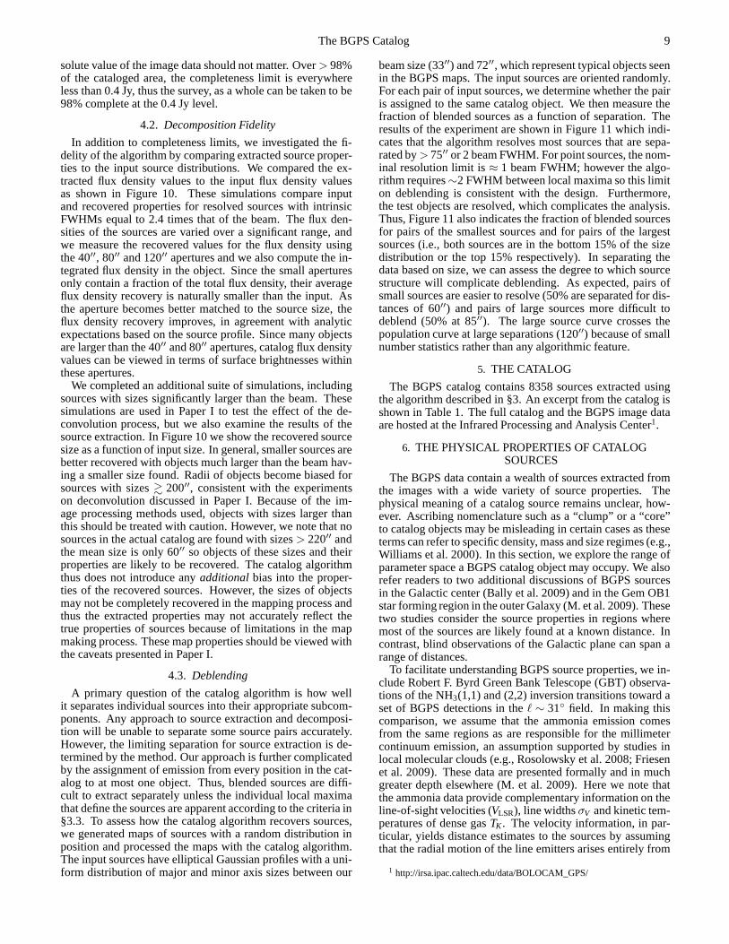
Figure 15 presents the total flux density extracted from theimages in catalog sources as a function of coordinates in theGalactic plane. In total, the catalog sources contain 11.9 kJyof flux density. Difficulties in recovery of large scale struc-ture notwithstanding, this represents the emission profileofthe Galaxy along the longitude and latitude direction.

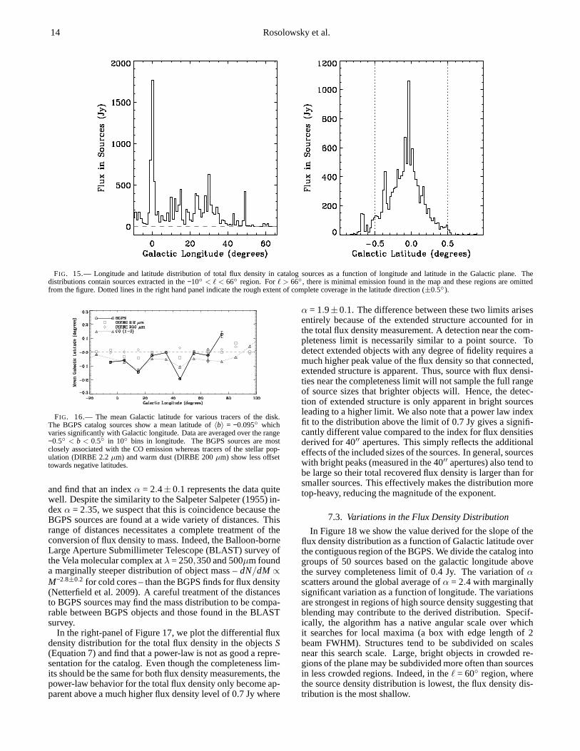
The right-hand panel of Figure 15 shows that the distribu-tion of flux density in sources peaks at the flux-weighted mean〈b〉 = −0.095±0.001 degrees. Such an offset was also seen inthe ATLASGAL survey of the 12 < b < −30 region of theGalactic plane atλ=870µm (Schuller et al. 2009). They spec-ulated that the offset may result from the Sun being locatedslightly above the Galactic plane. To further investigate thispossibility, we examined the latitudinal flux density distribu-tion of BGPS sources as a function of longitude and comparedthese results to other tracers of the Galactic disk. In particu-lar, we compared the flux density weighted values of the meanlatitude for objects in our catalog to the COBE/DIRBE dataat λ = 2.2 µm and 200µm (Hauser et al. 1998) and the inte-grated12CO (1-0) data of Dame et al. (2001). The results ofthe comparison are shown in Figure 16. For all data sets, weonly compute the flux-density weighted average latitude overthe range−0.5 < b < 0.5 which is the latitude range overwhich the BGPS is spatially complete. The data are averaged

The BGPS Catalog 13

FIG. 13.— Mass estimates for BGPS sources as a function of line-of-sight distance (left) and flux density (right). The massesare derived from a combinationof the BGPS data (for dust continuum flux densities) and ammonia data (for gas temperatures and kinematic distances) for matched sources in theℓ = 32 field.This figure highlights the wide range in the masses of objectsrecovered in the BGPS catalog.

FIG. 14.— Radius (left) and density (right) estimates for BGPS catalog objects matched with ammonia observations in theℓ = 32 field. Like Figure 13, agiven object is plotted twice for possible near and far kinematic distance estimates. The dotted line indicates the projected size forθR = 33′′ (1 beam FWHM) inthe left-hand panel. In the right-hand panel, the dotted line indicates the behavior for a source withS= 0.15 Jy =5σ andθR = 33′′. Sources can appear below theθR = 33′′ line because the beam deconvolution (Equation 6).

in 10 bins. The offset of BGPS sources appears at nearlyall Galactic longitudes, but is most pronounced towards theGalactic center (−10 < ℓ < 25). The CO (1-0) data followa similar trend with a significant offset towards negative lati-tudes. We verified that the effects persist in the CO data if theaveraging range is expanded to larger latitudes (foregroundemission from the Aquila rift affects the averaging for largelatitude ranges|b| < 5). We also note that the emission pro-files from the DIRBE data do not follow the offset trends seenin the millimeter continuum or the CO. The DIRBE 2.2µmdata primarily traces emission from stellar photospheres andis affected by dust extinction and the 200µm traces warmdust emission. Both of these emission features show a moresymmetrical distribution around the Galactic midplane thando those tracers associated with the molecular gas. We con-clude that the offsets towards negative latitude are primarilyassociated with the molecular ISM. The significant variationswith the mean offset are likely the result of individual starforming structures rather than a global property of all Galactic

components. For example, the large negative excursion in the40 < ℓ < 50 bin is due to the W51 star formation complex at(49.5,−0.4). At ℓ > 60, the space density of BGPS sourcesdrops sharply, so the effects are dominated by the particulardistribution of the dense gas within the molecular complex.Specifically, in theℓ ∼ 70 region, there are more dense gasstructures atb > 0 in the Cygnus X and Cygnus OB 7 regionthan there are atb< 0, while the lower density molecular gasdoes not exhibit this small-number effect.

7.2. The Flux Density Distribution of BGPS Sources

In Figure 17 we present two representations of the fluxdensity distribution for objects in the BGPS catalog. Theflux density distribution in 40′′ apertures is shown in the lefthand panel and follows a power-law form over nearly threeorders of magnitude in flux density from the point sourcecompleteness limit to the upper flux density limit in the sur-vey. We have fit a power law to the approximation to thedifferential flux density spectrumdN/dS≈ ∆N/∆S∝ S−α

14 Rosolowsky et al.

FIG. 15.— Longitude and latitude distribution of total flux density in catalog sources as a function of longitude and latitude in the Galactic plane. Thedistributions contain sources extracted in the−10 < ℓ < 66 region. Forℓ > 66, there is minimal emission found in the map and these regionsare omittedfrom the figure. Dotted lines in the right hand panel indicatethe rough extent of complete coverage in the latitude direction (±0.5).

FIG. 16.— The mean Galactic latitude for various tracers of the disk.The BGPS catalog sources show a mean latitude of〈b〉 = −0.095 whichvaries significantly with Galactic longitude. Data are averaged over the range−0.5 < b < 0.5 in 10 bins in longitude. The BGPS sources are mostclosely associated with the CO emission whereas tracers of the stellar pop-ulation (DIRBE 2.2µm) and warm dust (DIRBE 200µm) show less offsettowards negative latitudes.

and find that an indexα = 2.4±0.1 represents the data quitewell. Despite the similarity to the Salpeter Salpeter (1955) in-dexα = 2.35, we suspect that this is coincidence because theBGPS sources are found at a wide variety of distances. Thisrange of distances necessitates a complete treatment of theconversion of flux density to mass. Indeed, the Balloon-borneLarge Aperture Submillimeter Telescope (BLAST) survey ofthe Vela molecular complex atλ = 250,350 and 500µm founda marginally steeper distribution of object mass –dN/dM ∝M−2.8±0.2 for cold cores – than the BGPS finds for flux density(Netterfield et al. 2009). A careful treatment of the distancesto BGPS sources may find the mass distribution to be compa-rable between BGPS objects and those found in the BLASTsurvey.

In the right-panel of Figure 17, we plot the differential fluxdensity distribution for the total flux density in the objects S(Equation 7) and find that a power-law is not as good a repre-sentation for the catalog. Even though the completeness lim-its should be the same for both flux density measurements, thepower-law behavior for the total flux density only become ap-parent above a much higher flux density level of 0.7 Jy where

α = 1.9±0.1. The difference between these two limits arisesentirely because of the extended structure accounted for inthe total flux density measurement. A detection near the com-pleteness limit is necessarily similar to a point source. Todetect extended objects with any degree of fidelity requiresamuch higher peak value of the flux density so that connected,extended structure is apparent. Thus, source with flux densi-ties near the completeness limit will not sample the full rangeof source sizes that brighter objects will. Hence, the detec-tion of extended structure is only apparent in bright sourcesleading to a higher limit. We also note that a power law indexfit to the distribution above the limit of 0.7 Jy gives a signifi-cantly different value compared to the index for flux densitiesderived for 40′′ apertures. This simply reflects the additionaleffects of the included sizes of the sources. In general, sourceswith bright peaks (measured in the 40′′ apertures) also tend tobe large so their total recovered flux density is larger than forsmaller sources. This effectively makes the distribution moretop-heavy, reducing the magnitude of the exponent.

7.3. Variations in the Flux Density Distribution

In Figure 18 we show the value derived for the slope of theflux density distribution as a function of Galactic latitudeoverthe contiguous region of the BGPS. We divide the catalog intogroups of 50 sources based on the galactic longitude abovethe survey completeness limit of 0.4 Jy. The variation ofαscatters around the global average ofα = 2.4 with marginallysignificant variation as a function of longitude. The variationsare strongest in regions of high source density suggesting thatblending may contribute to the derived distribution. Specif-ically, the algorithm has a native angular scale over whichit searches for local maxima (a box with edge length of 2beam FWHM). Structures tend to be subdivided on scalesnear this search scale. Large, bright objects in crowded re-gions of the plane may be subdivided more often than sourcesin less crowded regions. Indeed, in theℓ = 60 region, wherethe source density distribution is lowest, the flux density dis-tribution is the most shallow.

The BGPS Catalog 15

FIG. 17.— Flux density number distribution for objects identified in the BGPS. The left-hand panel shows the flux density distribution for 40′′ apertures (S40)while the right-hand panel shows the total flux density associated with objects (S). We estimate the power law that best fits each distribution for flux densitiesabove the peak in the distribution. Note that the source distributions shown are estimators ofdN/dS, not dN/d(log M), although the bin widths used to derivethe distributions vary logarithmically.

FIG. 18.— Power-law index on the flux density distribution as a function ofGalactic longitude, derived for groups of 50 sources above the survey com-pleteness limit of 0.4 Jy. The flux densities are measured in 40′′ aperturesacross the Galactic plane.

7.4. Size Distribution of Sources

The measured sizes of sources varies significantly for theBGPS sources. We plot the distribution of source sizes andaspect ratios in Figure 19 for the catalog sources. We showthe major axis size (ησma j whereη = 2.4) determined fromthe moment method and the deconvolved angular radius ofthe source (θR), which includes both major and minor axes(Equation 6). Because of the deconvolution, the radiusθR canbe smaller than the beam size. However, we also note thatsome of the major axis sizes are also smaller than the beamsize. This results from applying moment methods without ac-counting for all emission down to theI = 0 level. The clipat 1σ truncates the low-significance band of emission aroundthe sources. For faint sources, the truncation will clip a sig-nificant fraction of the emission resulting in an underestimateof the source size. While this effect can be corrected for, werefrain from doing so since such corrections require extrapo-lating the behavior of the sources below the noise floor in theimages.

We also present data for the aspect ratios of the catalogsources defined asσma j/σmin. Both the radii and the aspectratios show a peaked distribution with an exponential decline.The typical source in the BGPS has a major axis size of 60′′

and a minor axis size of 45′′. However, there are significantnumbers of large-aspect-ratio sources which represents asym-

metric clump structure and, for faint sources, the prevalenceof filamentary structure in the survey.

8. SUMMARY

We present a catalog of 8358 sources extracted from theBolocam Galactic Plane Survey (BGPS, Aguirre et al. 2009).The BGPS is a survey of the Galactic Plane from−10 <ℓ < 90.5 with extensions into the outer Galaxy. The catalogis generated with an automated source extraction algorithm,Bolocat, that is designed for wide-field Bolocam mapping.The algorithm mimics a by-eye identification of sources inthe BGPS. The catalog products are formulated to allow easyfollow-up since many of the objects in the BGPS are relativelyunexplored.

The Bolocat algorithm identifies sources based on their sig-nificance with respect to a local estimate of the noise in theBGPS maps. Regions with high significance are then subdi-vided into individual sources based on the presence of localmaxima within the region. Each pixel in the BGPS image isassigned to at most one catalog source using a seeded water-shed, similar to the Clumpfind (Williams et al. 1994) or SEx-tractor algorithms (Bertin & Arnouts 1996). The propertiesof the BGPS sources are measured using the moments of theimages for each of the assigned sources.

We have conducted tests of the Bolocat algorithm using ar-tificial sources injected into observations in the survey fields.The Bolocat algorithm extracts sources with a 99% complete-ness limit of 5σ whereσ is the local RMS of the noise. Sincethe noise varies across the BGPS fields, the 98% complete-ness limit for the survey is 0.4 Jy, set by the highest noisefields.

Using spectroscopic observations of the NH3(1,1) inversiontransition, we have characterized several of the BGPS sourcesnearℓ = 32. We find that the objects in the catalog are likelybest described asclumps(Williams et al. 2000), though thereis substantial variation in the properties of the sources. Sincethe catalog is generated using a significance threshold, anysource that produces a signal> 5σ in the 33′′ beam size ofthe instrument will be detected. Hence, both nearby, small,low-mass objects and distant, large, high-mass objects canbedetected with similar flux densities.

We find the flux density distribution of sources in the BGPSfollows a power-law form. The flux densities of objects ex-

16 Rosolowsky et al.

FIG. 19.— Distributions of source angular sizes (left) and aspect ratios (right) in the BGPS catalog. In the left panel, the gray shaded histogram indicates themajor axis size of the sources derived from the moment methods. The black line-filled histogram shows the distribution ofthe deconvolved radii for the sources.The vertical line is plotted at the FWHM of the beam. In the right panel, the distribution plots the major-to-minor aspectratio for the moments of the source.

tracted in a 40′′ aperture follows a power-law over nearlythree orders of magnitude:dN/dS40 ∝ S−2.4±0.1

40 . We also findthat the mean Galactic latitude of objects in the survey liesat〈b〉 = −0.095±0.001, with some variation across the surveyregion according to the presence of large star-forming com-plexes.

The BGPS is supported by the National Science Foun-dation through the NSF grant AST-0708403. ER acknowl-edges partial support from an NSF AAP Fellowship (AST-0502605) and a Discovery Grant from NSERC of Canada.

NJE and MKN acknowledge support from the NSF grantAST-0607793. We acknowledge the cultural role and rever-ence that the summit of Mauna Kea has within the Hawaiiancommunity. We are fortunate to conduct observations fromthis mountain. The Green Bank Telescope is operated by theNational Radio Astronomy Observatory. The National RadioAstronomy Observatory is a facility of the National ScienceFoundation operated under cooperative agreement by Associ-ated Universities, Inc.

Facilities: CSO (Bolocam) GBT (K-band/ACS)

REFERENCES

Aguirre, J., A., G., M., D., Drosback, M., Bally, J., Battersby, C., Bradley,E., Cyganowski, C., Dowell, D., Evans, II, N. J., Glenn, J., Harvey, P. M.,Rosolowsky, E. W., Stringfellow, G., Walawender, J., & Williams, J. P.2009, ApJ, submitted

Bally, J., Aguirre, J., Battersby, C., Bradley, E., Cyganowski, C., Dowell, D.,Drosback, M., M., D., Evans, II, N. J., A., G., Glenn, J., Harvey, P. M.,Mills, E., Rosolowsky, E., Stringfellow, G., Walawender, J., & Williams,J. P. 2009, ApJ, submitted

Bertin, E. & Arnouts, S. 1996, A&AS, 117, 393Dame, T. M., Hartmann, D., & Thaddeus, P. 2001, ApJ, 547, 792Dougherty, E. 1992, An Introduction to Morphological ImageProcessing

(Bellingham: SPIE Optical Engineering Press)Enoch, M. L., Glenn, J., Evans, II, N. J., Sargent, A. I., Young, K. E., &

Huard, T. L. 2007, ApJ, 666, 982Enoch, M. L., Young, K. E., Glenn, J., Evans, N. J., Golwala, S., Sargent,

A. I., Harvey, P., Aguirre, J., Goldin, A., Haig, D., Huard, T. L., Lange, A.,Laurent, G., Maloney, P., Mauskopf, P., Rossinot, P., & Sayers, J. 2006,ApJ, 638, 293

Evans, II, N. J. 1999, ARA&A, 37, 311Friesen, R. K., Di Francesco, J., Shirley, Y. L., & Myers, P. C. 2009, ArXiv

e-printsGlenn, J., Ade, P. A. R., Amarie, M., Bock, J. J., Edgington, S. F., Goldin,

A., Golwala, S., Haig, D., Lange, A. E., Laurent, G., Mauskopf, P. D.,Yun, M., & Nguyen, H. 2003, in Presented at the Society of Photo-Optical Instrumentation Engineers (SPIE) Conference, Vol. 4855, Societyof Photo-Optical Instrumentation Engineers (SPIE) Conference Series, ed.T. G. Phillips & J. Zmuidzinas, 30–40

Hauser, M. G., Arendt, R. G., Kelsall, T., Dwek, E., Odegard,N., Weiland,J. L., Freudenreich, H. T., Reach, W. T., Silverberg, R. F., Moseley, S. H.,Pei, Y. C., Lubin, P., Mather, J. C., Shafer, R. A., Smoot, G. F., Weiss, R.,Wilkinson, D. T., & Wright, E. L. 1998, ApJ, 508, 25

Jackson, J. M., Rathborne, J. M., Shah, R. Y., Simon, R., Bania, T. M.,Clemens, D. P., Chambers, E. T., Johnson, A. M., Dormody, M.,Lavoie,R., & Heyer, M. H. 2006, ApJS, 163, 145

Johnstone, D., Wilson, C. D., Moriarty-Schieven, G., Joncas, G., Smith, G.,Gregersen, E., & Fich, M. 2000, ApJ, 545, 327

Kauffmann, J., Bertoldi, F., Bourke, T. L., Evans, II, N. J.,& Lee, C. W. 2008,A&A, 487, 993

M., D., Rosolowsky, E. W., Evans, II, N. J., Cyganowski, C., Aguirre,J., Bally, J., Battersby, C., Bradley, E., Dowell, D., Drosback, M., A.,G., Glenn, J., Harvey, P. M., Merello, M., Schlingman, W., Shirley, Y.,Stringfellow, G., Walawender, J., & Williams, J. P. 2009, /apj, submitted

Moore, T. J. T., Shipman, R. F., Plume, R., Hoare, M. G., & Jps InternationalCollaboration. 2005, in Protostars and Planets V, 8370–+

Motte, F., Andre, P., & Neri, R. 1998, A&A, 336, 150Netterfield, C. B., Ade, P. A. R., Bock, J. J., Chapin, E. L., Devlin, M. J.,

Griffin, M., Gundersen, J. O., Halpern, M., Hargrave, P. C., Hughes, D. H.,Klein, J., Marsden, G., Martin, P. G., Mauskopf, P., Olmi, L., Pascale,E., Patanchon, G., Rex, M., Roy, A., Scott, D., Semisch, C., Thomas, N.,Truch, M. D. P., Tucker, C., Tucker, G. S., Viero, M. P., & Wiebe, D. V.2009, ArXiv e-prints

Noriega-Crespo, A. & Molinari, S. 2008, in Bulletin of the AmericanAstronomical Society, Vol. 40, Bulletin of the American AstronomicalSociety, 271–+

Press, W. H., Teukolsky, S. A., Vetterling, W. T., & Flannery, B. P. 1992,Numerical recipes in C. The art of scientific computing (Cambridge:University Press, |c1992, 2nd ed.)

Reid, M. J., Menten, K. M., Zheng, X. W., Brunthaler, A., Moscadelli, L.,Xu, Y., Zhang, B., Sato, M., Honma, M., Hirota, T., Hachisuka, K., Choi,Y. K., Moellenbrock, G. A., & Bartkiewicz, A. 2009, ArXiv e-prints

Rosolowsky, E. W., Pineda, J. E., Foster, J. B., Borkin, M. A., Kauffmann, J.,Caselli, P., Myers, P. C., & Goodman, A. A. 2008, ApJS, 175, 509

Salpeter, E. E. 1955, ApJ, 121, 161Schuller, F., Menten, K. M., Contreras, Y., Wyrowski, F., Schilke, P.,

Bronfman, L., Henning, T., Walmsley, C. M., Beuther, H., Bontemps, S.,Cesaroni, R., Deharveng, L., Garay, G., Herpin, F., Lefloch,B., Linz, H.,Mardones, D., Minier, V., Molinari, S., Motte, F., Nyman, L.., Reveret, V.,Risacher, C., Russeil, D., Schneider, N., Testi, L., Troost, T., Vasyunina, T.,Wienen, M., Zavagno, A., Kovacs, A., Kreysa, E., Siringo, G., & Weiss, A.2009, ArXiv e-prints

Williams, J. P., Blitz, L., & McKee, C. F. 2000, Protostars and Planets IV, 97Williams, J. P., de Geus, E. J., & Blitz, L. 1994, ApJ, 428, 693Yoo, T., ed. 2004, Insight Into Images ’Principles and Practice for

Segmentation, Registration and Image Analysis’ (A K PetersLtd.)Young, K. E., Enoch, M. L., Evans, II, N. J., Glenn, J., Sargent, A., Huard,

T. L., Aguirre, J., Golwala, S., Haig, D., Harvey, P., Laurent, G., Mauskopf,P., & Sayers, J. 2006, ApJ, 644, 326