The big chaos solution to the netflix grand prize

The BigChaos Solution to the Netflix Grand Prize

Andreas Toscher and Michael Jahrer

commendo research & consultingNeuer Weg 23, A-8580 Koflach, Austria

andreas.toescher,[email protected]

Robert M. Bell∗

AT&T Labs - ResearchFlorham Park, NJ

September 5, 2009

1 Introduction

The team BellKor’s Pragmatic Chaos is a combined team of BellKor, Pragmatic Theory and BigChaos.BellKor consists of Robert Bell, Yehuda Koren and Chris Volinsky. The members of Pragmatic Theoryare Martin Piotte and Martin Chabbert. Andreas Toscher and Michael Jahrer form the team BigChaos.BellKor won the Progress Prize 2007 [4]. The Progress Prize 2008 was won by the combined efforts ofBellKor and BigChaos [5][17].

The documentation of the Netflix Grand Prize consists of three parts. In this document we focus onthe contribution of BigChaos to the combined Grand Prize Solution.

The document is organized as follows: In Section 2 we describe the Netflix dataset and importantstatistical properties, followed by a detailed explanation of the training procedure of our predictors inSection 3. Section 4 defines the notation, which we use throughout this document. The algorithmicdetails can be found in Section 5. In order to combine the predictors of BigChaos and the whole teamto form a final prediction, we used a combination of nonlinear probe blending and linear quiz blending.The nonlinear probe blending techniques are described in Section 6, the linear quiz blend is described inSection 7. In Appendix A a detailed list of all used predictors is attached.

2 The Netflix Prize Dataset

The dataset consists of 5-star ratings on 17770 movies and 480189 anonymous users. It was collected byNetflix in a period of approximately 7 years. In total, the number of ratings is 100480507; the probe setof size 1408395 is a subset of them. The goal of the contest is to predict the qualifying set (size: 2817131samples) and achieve a RMSE score of at least 0.8563 on the quiz subset, to get qualified for the GrandPrize. The quiz set is an unknown 50% random subset of the qualifying set. The judging criteria forwinning the Netflix Grand Prize is the four digits rounded RMSE score on the test set (remaining 50%).In the case of a tie the earliest submission wins. The probe set has equal statistical properties as thequalifying set. Furthermore it is used as a hold-out set during the competition. Full description of therules can be found under [1].

∗The author contributed Section 7

1

Training set Qualifying setProbe set

Quiz Test

cnt=100,480,507 cnt=1408395 cnt=2817131

50% 50%

Leaderboard feedback

Figure 1: The Netflix Prize dataset in detail. Ratings are available for the training set. Netflix acceptspredictions for the qualifying set, the feedback (4 digit precision) is calculated on a 50% random subsetof the qualifying set, the quiz set.

100

101

102

103

104

0

2000

4000

log(support)

user

cou

nt

0 500 1000 1500 20000

1

2

3x 10

5

days (from 1998 to 2005)

ratin

g co

unt

100

101

102

0

5

10x 10

6

log(frequency)

num

ber

of u

ser−

days

Figure 2: Effects in the rating dataset. First row: User support is the number of votes given from auser. The mode of the user support is on 19 votes, where the average number of votes is 200. Secondrow: More ratings at the end of the timeline. Third row: Frequency is the number of votes per day peruser. Most users gave one or two votes per day. The idea to explore the frequency effect was introducedby our colleagues from Pragmatic Theory.

3 Frameworks

3.1 Optimize the Predictors Individually on the Probe Set

The solutions of the Netflix Progress Prizes of 2007 and 2008 had a focus on the accuracy of the individualcollaborative filtering algorithms. Blending techniques were used to combine the independently trainedpredictors. The predictors were trained to minimize the RMSE on the probe set. First, the probe setis excluded from the training data. The model gets trained to minimize the probe set. For gradientdescent methods this means that the training has to stop when the RMSE on the probe set is minimal.Then predictions are stored for the probe set. Afterwards, the probe set gets included into the trainingdata and the training starts again, with exactly the same parameters and initial conditions. After the

2

second training stage, we generate predictions for the qualifying set. These predictions achieve a 0.0030to 0.0090 better quiz RMSE, compared to their probe RMSE, thanks to expanding the training set.

For every algorithm run, the outcome is a predictor for the probe and qualifying set, which can beused in probe blending, see Section 6. The individual predictor is optimized to achieve the lowest possibleprobe RMSE. Some algorithms are based on the residuals of others. To calculate the residual error weuse the training set predictions of the trained predictor as shown in Figure 3.

3.2 Optimize the Blend

A key observation with ensemble methods is that it is not optimal to minimize the RMSE of the individualpredictors. Only the RMSE of the ensemble counts. Thus the predictors which achieve the best blendingresults are the ones, which have the right balance between being uncorrelated to the rest of the ensembleand achieving a low RMSE individually. An ideal solution would be to train all models in parallel andtreat the ensemble as one big model. The big problem is that training 100+ models in parallel andtuning all parameters simultaneously is computationally not feasible.

We approximate this ideal solution by training the models one after another, where each model triesto achieve best results when blended with all preceding models. So the focus shifts from looking at theRMSE of an individual predictor to the RMSE of a blended ensemble. In the following, we refer to theprobe RMSE of a linear blend with all preceding predictors as “blend RMSE”.

Each predictor tries to achieve best results when it is blended with all preceding ones. Therefore weneither reformulate the error function, nor change any learning rules. We just determine the numberof training epochs, which give the best blending improvement. For the first algorithm this means tostop the training when the blend with a constant predictor reaches the minimum. The training of thesecond algorithm is stopped, when the blend with the first and a constant predictor is minimal. Thusevery subsequent predictor stops the training when the blending result with the preceding predictors(including the constant predictor) is minimal. Algorithm 1 provides a pseudo code description of thetraining’s process for one predictor.

All meta parameters, which are tuned automatically, are tuned in order to minimize the blendingRMSE instead of the probe RMSE of the individual predictor.

Train Set

Predicted Train Set

CF Model

Figure 3: This figure visualizes the standard way for calculating residuals. A CF algorithm is trainedon the whole training set and used to predict the training set. In the frameworks 3.1 and 3.2 we alwaysused this method for calculating residuals.

For large ensembles we observed that gradient descent based algorithms tend to train more and moreepochs. Therefore, the models are trained over the point of probe minimum. Thus, the RMSE of theindividual predictors rises, whereas the RMSE of the ensemble lowers.

An interesting issue is the time and space complexity of this training process. As described abovethe major difference to the standard training framework is to calculate a blend RMSE instead of theprobe RMSE. In the case of a gradient descent algorithm the blend RMSE gets only calculated at theend of each epoch in the training phase. In the retraining phase the calculation of the blend RMSEis not necessary, because the number of needed training epochs were determined in the first trainingphase. So the time and space complexity does not change for the retraining. In order to calculate theblend RMSE one has to keep the probe predictions of all preceding predictors in memory (about 5.6MB per file in single precision), so the memory requirement rises linearly with the number of predictors.The time complexity for solving the linear equation system rises with the third power dependent on the

3

number of preceding predictors. For our 101 predictors the calculation of a single blend RMSE can bedone in about 1 second, on a modern quad core processor.

The predictor list in Appendix A reports 101 results, which are consecutively optimized to minimizethe blend RMSE. Predictions are not clipped. This helps the final blender to improve accuracy. Al-gorithms with meta parameters, which have strong impact on the outcome, like various MovieKNNs,Global Effects or Global Time Effects, are useful to minimize the blend RMSE. The residuals are alwayscalculated as shown in Figure 3.

Input: A matrix P with all previous probe predictions. P always includes a constant predictor (acolumn with ones).

Exclude the Probe ratings r from the training set.1

Initialize the weights.2

RMSEbest =∞3

RMSEepoch = 10004

epochs = 05

while RMSEepoch ≤ RMSEbest do6

Train one epoch.7

if RMSEepoch ≤ RMSEbest then8

RMSEbest = RMSEepoch9

Save the current weights.10

end11

Predict the probe set p.12

Merge current probe prediction p and previous predictions: X = [P p]13

Calculate blending weights: w = (XTX)−1XT r14

Calculate prediction of the current blend: p = X ·w15

Calculate the RMSE of the blend: RMSEepoch =√

1R

∑Ri=1 (pi − ri)2; ri is probe rating i, R16

is #ratings in the probe setepochs = epochs+ 117

end18

Load the weights.19

Generate predictions for the probe set.20

Insert the probe set into the training set.21

Initialize the weights (use the same random seed as for the first initialization).22

while epochs > 0 do23

Train one epoch.24

epochs = epochs− 125

end26

Generate predictions for the qualifying set.27

Algorithm 1: Pseudo code for training a single predictor with gradient descent and stopping onthe optimal blending improvement (Section 3.2 and 3.3). In contrast to the standard proceduredescribed in 3.1 where the training is stopped on the probe minimum, here the training is stoppedwhen the resulting predictor achieves best blending results. This means we do normal epoch wisetraining and calculate the blending RMSE after each epoch and stop the training when the predictorachieves the best blending results with all preceding predictors. After finding the optimal numberof training epochs, we include the probe set and retrain the model using the same initial weights.After the retraining we generate predictions for the qualifying set. As a result we get a predictorwith probe and qualifying predictions (like in 3.1), which can be used for any sort of probe blending.

3.3 Optimize the Blend and Correct Residuals

Some of our models deliver very good results on the residuals of others. A well known combination areneighborhood based approaches on the residuals of Restricted Boltzmann Machines (RBM). The firsttwo frameworks are not ideal in this setup. We calculate the residuals for the training set, with a modelwhich was trained on the same ratings (Figure 3). In order to correct this deficiency, we calculate herethe residuals with a k-fold cross validation (Figure 4). This brings relatively much computational effortto train each individual model, hence the number of results from this framework results in 10 predictors

4

(10 complete algorithm runs).

TK

T1

T2

T3

T2

T3

T1

TK

M2

M3

M1

MK

Train Set

Predicted Train Set

Figure 4: This figure visualizes the idea of “correct residuals”. We split the train set into K disjoint setsT1 to TK of equal size and train K different CF models M1 to MK . The first model M1 uses the ratingsof the sets T2 to TK for training and generates predictions for the set T1. The second model M2 excludesthe set T2 in the training phase, and calculates predictions for this set. Each rating in the training setis predicted by 1 model. Each rating in the probe and qualifying set is predicted by 34 models. Thepredictions for the probe and the qualifying set are linear blends of all K models.

As in the previous framework, we train the models to minimize the blend RMSE. We always useK = 34, this means 34 models are trained and retrained for generating one predictor. Details can befound in Figure 4. The reason for choosing K = 34 is the size of our cluster. We have access to a clusterwith 34 compute nodes with each having 4 GB of main memory, and a single head node with 8 GB ofmain memory. In our experience higher values for K achieve better results, but also the computationalefforts increase linearly with K.

4 Notation

The following mathematical notation is used throughout the document. For the description of somealgorithms we need additional definitions, which will be made on demand.

• u, v ... users

• i, j ... movies (items)

• rui ... real rating of user u for item i

• tui ... the date (days since 01.01.1998) when user u rated item i

• rui, rui, rui ... prediction of user u for item i

• N(u) ... set of all items, rated by user u including those with unknown ratings on the qualifyingset

• N(i) ... set of all users, which rated item i including those with unknown ratings on the qualifyingset

• R(u) ... set of items, rated by user u (known ratings)

• R(i) ... set of users, which rated item i (known ratings)

• R(u, i) ... set of k items nearest (largest item-item correlation) to item i which were rated by useru

• α, β, γ, δ, ε, ζ, θ, ϑ, κ, ξ ... meta parameters, which can be tuned (small Greek letters)

• For gradient descent based algorithms: learning rate η, regularization λ. Throughout the document,when we use the term regularization, we mean L2-regularization.

5

• Vectors or matrices have bold face characters, such as P, Q, pi, qu, yi

• In SVD models item features are pi, user features qu, asymmetric movie features yi, biases are µ.If we have more than one item or user feature, we denote it by p(1)

i and p(2)i .

5 Collaborative Filtering Algorithms

This section describes all different collaborative filtering (CF) algorithms, which we used in the contest.Some of them are already covered in [17], but still listed here, because most of our Progress Prize 2008predictors are used in the final blend. For clarity, we state for every algorithm whether it is new, modifiedor exactly the same as used for the Progress Prize 2008. All the produced predictors are exactly listedin Appendix A, including all used parameters.

5.1 Automatic Parameter Tuning - APT

For some algorithms an automatic tuning of the involved meta parameters is needed. We use APT1and APT2 methods as described in [17]. Both methods are simple direct search methods, which workwithout the need of a gradient. APT1 randomly changes single parameters and keeps the changes, whenthe error improves. APT2 is a structured coordinate search.

APT1 and APT2 are unchanged since the progress prize 2008.

5.2 Movie KNN

Neighborhood based approaches are very popular collaborative filtering methods. The Netflix Prize hasclearly shown that these methods can easily be beaten in terms of speed and accuracy by simple factormodels. As individual models, they do not achieve outstanding low RMSE values, but in an ensembleof methods they work very well. In the first year of the competition it was shown that they yield greatresults on the residuals of RBMs. For the Progress Prize 2008 we used a variety of KNN models on theresiduals of nearly every algorithm.

Our focus shifted from improving a single predictor or residual-chain of predictors to optimizing theRMSE of the ensemble of predictors. In this context the KNN models do an even better job. Themeta parameters are very powerful and help to produce diverse predictors, which blend well. Automaticparameter tuning can do this automatically.

5.2.1 Correlations

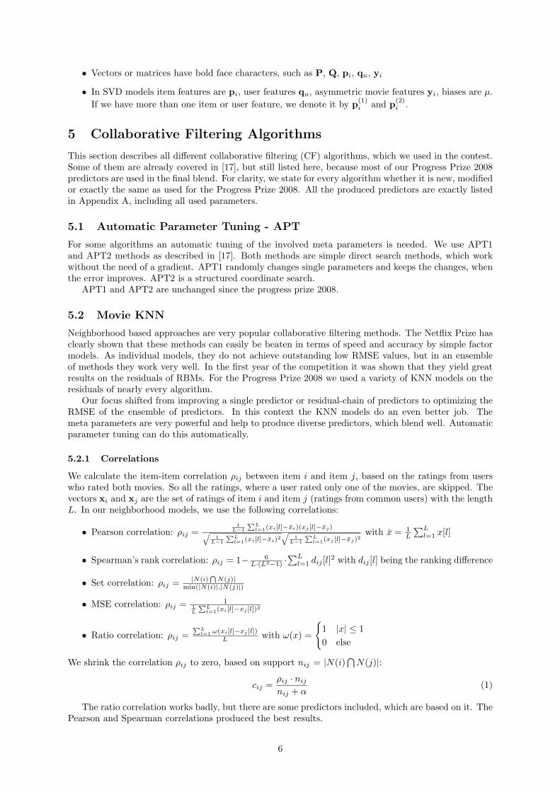
We calculate the item-item correlation ρij between item i and item j, based on the ratings from userswho rated both movies. So all the ratings, where a user rated only one of the movies, are skipped. Thevectors xi and xj are the set of ratings of item i and item j (ratings from common users) with the lengthL. In our neighborhood models, we use the following correlations:

• Pearson correlation: ρij =1

L−1

PLl=1(xi[l]−xi)(xj [l]−xj)q

1L−1

PLl=1(xi[l]−xi)2

q1

L−1

PLl=1(xj [l]−xj)2

with x = 1L

∑Ll=1 x[l]

• Spearman’s rank correlation: ρij = 1− 6L·(L2−1) ·

∑Ll=1 dij [l]

2 with dij [l] being the ranking difference

• Set correlation: ρij = |N(i)TN(j)|

min(|N(i)|,|N(j)|)

• MSE correlation: ρij = 11L

PLl=1(xi[l]−xj [l])2

• Ratio correlation: ρij =PL

l=1 ω(xi[l]−xj [l])

L with ω(x) =

1 |x| ≤ 10 else

We shrink the correlation ρij to zero, based on support nij = |N(i)⋂N(j)|:

cij =ρij · nijnij + α

(1)

The ratio correlation works badly, but there are some predictors included, which are based on it. ThePearson and Spearman correlations produced the best results.

6

5.2.2 KNNMovieV3

This model is exactly the same as in the Progress Prize 2008:

cdateij = σ

(δ · cij · exp

(− | 4t |

β

)+ γ

)(2)

σ(x) =1

1 + exp(−x)(3)

rui =

∑j∈R(u,i) c

dateij ruj∑

j∈R(u,i) cdateij

(4)

| 4t | stands for days between the rating rui, which we are going to predict, and the past rating ruj .We use APT1 to tune this model.

5.2.3 KNNMovieV3-2

The KNNMovieV3 model is extended by 5 meta parameters: ζ, κ, ν, ϑ, ψ. These are used in order tomake the model more powerful and flexible. This modification was not part of the Progress Prize 2008:

cnewij = σ

(δ · sign(cij)|cij |ζ · exp

(− | 4t |

β

)+ γ

)(5)

σ(x) = κ · 11 + exp(−x)

+ ν (6)

L(x) =

x −ϑ ≤ x ≤ ϑϑ x > ϑ

−ϑ x < −ϑ(7)

rui = L

(ψ

∑j∈R(u,i) c

newij ruj∑

j∈R(u,i) cnewij

)(8)

In the frameworks 3.2 and 3.3 this model yields very good results. In these frameworks we do notoptimize the predictors individually, the predictors get optimized to give the best blending results. Incontrast to KNNMovieV3 we tune all parameters with APT2, which converges faster.

5.3 Time Dependence Models

Time dependence models account for an over time changing rating mean. We reported all details for theProgress Prize 2008 [17]. The over time changing user mean is called customer time dependence model[CTD] and the flipped version is referred to as movie time dependence model [MTD].

5.4 Restricted Boltzmann Machine - RBM

We use RBMs as described in [15]. Instead of mini batch updates as described in the paper, we usepure stochastic gradient ascent. In our progress prize paper [17], we refer to the conditional RBM withmultinomial visible units as RBMV3. The conditional RBM with Gaussian visible units is called RBMV5.The flipped version, where a movie is represented by the users who rated it, is called RBMV6.

The RBMs are unchanged since the Progress Prize 2008. In Section 6.10 we describe how to usethe low dimensional representation of users and items on the hidden units as additional features for theblending.

7

5.5 Global Effects - GE

Global Effects capture statistical corrections applied on user and item side, see [2]. We used them forpreprocessing and postprocessing on residuals of other algorithms. The prediction formula of the firstglobal effect (Movie effect) is given by

rui = θixui (9)

The value of xui is a static feature, where the value of θi is estimated by θi shrunken with α1

θi =θi |R(i)|

α1 + |R(i)|(10)

and θi results from a simple estimator from [2]

θi =

∑u∈R(i) ruixui∑u∈R(i) x

2ui

(11)

All other effects are similar. The explanatory variables (or the fixed features) xui are different for eacheffect. For “Movie effect” or “User effect” the xui are always 1. Thus, global effects can be seen as anSVD approach with either fixed movie of fixed user features. Large values of α shrink the predictiontowards 0. In Table 1 we list all used global effects. For some predictors we have not used all 16 effects,so we stated the exact number of used effects for every GE predictor. When not calculating xui on theresiduals of the previous GE, we denote this with “on raw residuals/ratings” in Table 1. In the thesecases the xui are calculated based on the raw ratings or residuals.

For the Progress Prize 2008 we reported 14 GE. In Table 1 we are listing 16, meaning we use 2 newones. They capture dependencies on the average of the residual directly. One major improvement overlast year’s implementation is that at the end of the stagewise fitting of optimal α shrinkage, we optimizethe parameter α on all effects simultaneously. This is done for 700 epochs with APT2. The runtime persearch epoch is about 1 minute. Global Effects are an effective way to optimize the blend RMSE whenapplied on residuals.

In the framework for minimizing the blend RMSE, we use two minimization steps in Global Effects.The first step optimizes the probe RMSE of the predictor itself, the second step minimizes the blend.This helps to find good start values of all α.

# effect shrinkage1 Movie effect α1

2 User effect α2

3 User effect: user x sqrt(time(user)) α3

4 User effect: user x sqrt(time(movie)) α4

5 Movie effect: movie x sqrt(time(movie)) α5

6 Movie effect: movie x sqrt(time(user)) α6

7 User effect: user x average(movie) α7

8 User effect: user x votes(movie) α8

9 Movie effect: movie x average(user) α9

10 Movie effect: movie x votes(user) α10

11 Movie effect: movie x avgMovieProductionYear(user) α11

12 User effect: user x productionYear(movie) α12

13 User effect: user x std(movie) α13

14 Movie effect: movie x std(user) α14

15 User effect: user x average(movie) (on raw residuals/ratings) α15

16 Movie effect: movie x average(user) (on raw residuals/ratings) α16

Table 1: Global Effects

5.6 Global Time Effects - GTE

Time varying global effects are called global time effects. Their detailed implementation with all formulasto derive a prediction model can be found in [17]. In Table 2 we list all used GTE. GTE benefit from

8

applying two movie and user effects as the first 4 effects. The algorithm has the ability to adapt thekernel width σ per effect. This helps to capture basic movie and user effects on different time scales. Thekernel width represents the size of the time-localized window. For the Progress Prize 2008 we reported19 GTE. These are getting refined and extended to become 24 single effects. The new effects are basedon:

• percentSingleVotes(user): Percentage of all rating days, where the user gives only one vote.

• avgStringlenTitle(user): The average length of the movie title voted by the user.

• ratingDateDensity(user): The rating time span (last minus first rating day) divided by the numberof rating days (the days on which the user has given at least one rating).

• percentMovieWithNumberInTitle(user): The percentage of movies with numbers in the title votedby the user.

• ratingDateDensity(movie): The same on movie side.

User side effects need more computational effort (3 minutes per epoch), therefore we limit the au-tomatic parameter tuner APT2 to 120 epochs. On item side we use 400 search epochs. In contrast toGlobal Effects, optimizing all meta parameters simultaneously is not feasible, due to the huge runtime.However, Global Time Effects are a strong algorithm to minimize the blend RMSE in the ensemble.

# effect shrinkage kernel width0 Global time mean α0 σ0

1 Movie time effect α1 σ1

2 User time effect α2 σ2

3 Movie time effect α3 σ3

4 User time effect α4 σ4

5 User time effect: user x sqrt(time(user)) α5 σ5

6 User time effect: user x sqrt(time(movie)) α6 σ6

7 Movie time effect: movie x sqrt(time(movie)) α7 σ7

8 Movie time effect: movie x sqrt(time(user)) α8 σ8

9 User time effect: user x average(movie) α9 σ9

10 User time effect: user x votes(movie) α10 σ10

11 Movie time effect: movie x average(user) α11 σ11

12 Movie time effect: movie x votes(user) α12 σ12

13 Movie time effect: movie x avgMovieProductionYear(user) α13 σ13

14 User time effect: user x productionYear(movie) α14 σ14

15 User time effect: user x std(movie) α15 σ15

16 Movie time effect: movie x std(user) α16 σ16

17 User time effect: user x average(movie) (from previous effect) α17 σ17

18 Movie time effect: movie x average(user) (from previous effect) α18 σ18

19 Movie time effect: movie x percentSingleVotes(user) α19 σ19

20 Movie time effect: movie x avgStringlenTitle(user) α20 σ20

21 Movie time effect: movie x ratingDateDensity(user) α21 σ21

22 Movie time effect: movie x percentMovieWithNumberInTitle(user) α22 σ22

23 User time effect: user x stringlengthFromTitle(movie) α23 σ23

24 User time effect: user x ratingDateDensity(movie) α24 σ24

Table 2: Overview on 24 Global Time Effects

5.7 Weekday Effect - WE

This algorithm applies mean correction on weekdays. The detailed implementation can be found in [17].It is unchanged since the Progress Prize 2008.

9

5.8 Integrated Model - IM

The model with the highest reported accuracy was explained by team BellKor in the 2008 ProgressPrize report [5]. This was the inspiration of our Integrated Model. The aim of an integrated model is toexplain different effects in the data in one big model. All latent parameters are trained simultaneously bystochastic gradient descent. The training samples are ordered user wise. The asymmetric part receivesupdates after processing each user. Each latent vector has the same number of features. Time is measuredas days since 1/1/1998.

The prediction formula for our Integrated Model is

ruit = µ+ µ(1)i + µ

(2)i · dit + µ

(3)i,bin(t) + µ(1)

u + µ(2)u · dut + µ

(3)u,t + r

(1)uit + r

(2)uit + r

(3)uit + r

(4)uit (12)

Item time deviation:dit = dev(µ(t)

i , t) (13)

User time deviation:dut = dev(µ(t)

u , t) (14)

Non linear time deviation is defined by

dev(µ, t) = sign (t− µ) · |t− µ|0.5 (15)

The mean rating date of a user u:

µ(t)u =

1|R(u)|

∑j∈R(u)

tuj (16)

The mean rating date of an item i:

µ(t)i =

1|R(i)|

∑v∈R(i)

tvi (17)

The first item-user dot product accounts for complex user-item interactions with time:

r(1)uit =

(p(1)i + p(2)

i dit + p(3)i,bin(t)

)T q(1)u + q(2)

u dut + q(3)u,t +

1√|N(u)|

∑j∈N(u)

(y(1)j + y(2)

j djt + y(3)j,bin(t)

)(18)

The second part accounts for user-item interaction in frequency. The number of votes by user u on dayt is denoted by fut:

r(2)uit =

(p(4)i

)T (q(4)u + q(5)

u,fut

)(19)

The third part is a neighborhood approach, which models item-item interactions with time. The µ(g)i is

the item mean and µ(g)u the user mean. They are trained at the beginning and kept constant afterwards:

r(3)uit =

(p(5)i

)T 1√|R(i)|

∑j∈R(u)

(ruj − µ(g)i − µ

(g)u )

(y(4)j + y(5)

j djt

) (20)

The fourth part is a NSVD [13] with time:

r(4)uit =

(p(6)i + p(7)

i dit

)T 1√|N(u)|

∑j∈N(u)

(y(6)j + y(7)

j djt + y(8)j,bin(t)

) (21)

The user frequency fut is the number of votes from user u on day t. The timeline is divided into a fixednumber of bins, bin(t) selects the corresponding bin at time t. The exact number of bins is reported forevery predictor in the listing (Appendix A).

All parameters are initialized by uniformly drawing them from the interval [−1e − 3, 1e − 3]; alllearning rates η and regularizations λ are optimized by APT2 (1500 search epochs requiring approx. 2month on 3 GHz Intel Core2 with a latent feature size of 10). The small number of 10 latent features waschosen in order to minimize the runtime for optimization of all meta parameters. We use 10 equal timebins for capturing movie time effects for all integrated model results. The following learn parameterswere found by the auto-tuning process. We report 3 results in the predictor list, which have exactly the

10

following values as the learning parameters.

ηµi= 0.0017 λµi

= 8.2807e − 06 ηµu= 0.0013 λµu

= 0.0030 ηµi,bin(t) = 0.0017 λµi,bin(t) = 8.2807e − 06ηµu,t

= 0.0013 λµu,t= 0.0030 η

p(1)i

= 0.0016 λp(1)i

= 0.0328 ηp(2)i

= 0.0071 λp(2)i

= 0.1484 ηp(3)i,bin(t)

=

3.1342e − 05 λp(3)i,bin(t)

= 0.2090 ηp(4)i

= 0.0016 λp(4)i

= 0.0324 ηp(5)i

= 1.7027e − 04 λp(5)i

= 0.0243

ηp(6)i

= 4.7343e−04 λp(6)i

= 0.0128 ηp(7)i

= 2.3333e−04 λp(7)i

= 1.7976e−04 ηq(1)u

= 0.0057 λq(1)u

= 0.0274ηq(2)u

= 0.0055 λq(2)u

= 0.0110 ηq(3)u,t

= 0.0018 λq(3)u,t

= 0.0086 ηq(4)u

= 0.0138 λq(4)u

= 0.0063 ηq(5)u,fut

= 0.0024

λq(5)u,fut

= 5.1112e − 04 ηy(1)j

= 0.0017 λy(1)j

= 7.8809e − 04 ηy(2)j

= 4.0333e − 04 λy(2)j

= 9.3459e − 05

ηy(3)j,bin(t)

= 2.7478e−04 λy(3)j,bin(t)

= 0.0011 ηy(4)j

= 2.3063e−04 λy(4)j

= 0.0218 ηy(5)j

= 0.0021 λy(5)j

= 0.0372

ηy(6)j

= 0.0012 λy(6)j

= 0.0206 ηy(7)j

= 1.1255e−04 λy(7)j

= 0.0021 ηy(8)j,bin(t)

= 2.6278e−04 λy(8)j,bin(t)

= 0.0104

#features probeRMSE10 0.8966

Table 3: RMSE on the probe set for the Integrated Model. The automatic parameter tuner APT2optimizes the RMSE on the probe set until overfitting occurs.

5.9 Maximum Margin Matrix Factorization - MMMF

The maximum margin matrix factorization learns two K-dimensional factor matrices P, Q and 4 thresh-olds θu1 < θu2 < θu3 < θu4 for each user u. The prediction consists of only integer ratings:

rui =

1, pTi qu < θu1

2, θu1 ≤ pTi qu < θu2



5, else

(22)

The implementation is based on the description in [19]. We were not able to get a RMSE below 1.0 onthe probe set.

5.10 NSVD

This is one of the most important approaches to describe user via their rated items. Paterek [13] presentsthis model in 2007. The model has no explicit user features, so the number of parameters is reduced.

5.10.1 NSVD1

The model learns user and item biases and two sets of item features pi and qi:

rui = µi + µu + piT

1√|N(u)|

∑j∈N(u)

qj

(23)

A NSVD1 on raw ratings with 500 features achieves a probe RMSE of 0.933.

5.10.2 NSVD2

Simply using the same item features for pi and qi leads to the NSVD2 model:


1√|N(u)|

∑j∈N(u)

pj

(24)


11

5.10.3 NSVD1 Discrete - NSVDD

Item features qi describe the asymmetric user part in the NSVD1 model. To model the distribution ofdiscrete ratings, we introduce 5 separate item feature sets qi,d with d ∈ 1, 2, 3, 4, 5. A user is explainedvia a bag of movie rating features, but in contrast to NSVD1 we choose a different item feature vectorqi,d, based on the given ratings:


1√|R(u)|

∑j∈R(u)

qj,ruj

(25)


5.11 SBRAMF - Special Biased Regularized Asymmetric Matrix Factoriza-tion - and Extensions

Takacs et al. [16] suggest a special regularization schema for rating matrix factorization algorithms. Theidea is to account for the inverse dependency of regularization λ and learning rate η on the supportof user u and item i. By using much more trainable weights than examples (overparameterizing) andauto-tuning of the learning rates and regularizations of the SVD results in a very accurate model. Forexample the learning rate ηui can be expressed by following function:

ηui = p1 + p21

log(|R(u)|+ 1)+ p3

1√|R(u)|

+ p41

|R(u)|+ p5

1log(|R(i)|+ 1)

+ p61√|R(i)|

+ p71|R(i)|

(26)

The basic SVD model with biases is SBRMF

rui = µi + µu + piTqu (27)

In 2008, Koren extended the plain SVD model with implicit information 1√|N(u)|

∑j∈N(u) yj , which is

called SVD++ model [11]. In this model a user is represented by the user feature qu and a “bag ofitems” yi (the items rated by the user). SBRMF extended by the asymmetric part is equal to SVD++,which we call SBRAMF


qu +1√|N(u)|

∑j∈N(u)

yj

(28)

Add a user and movie time bias µu,t, µi,bin(t): SBRAMF-UTB

ruit = µi + µu + µu,t + µi,bin(t) + piT

qu +1√|N(u)|

∑j∈N(u)

yj

(29)

Add a user time feature q(2)u,t: SBRAMF-UTB-UTF

ruit = µi + µu + µu,t + µi,bin(t) + piT

q(1)u + q(2)

u,t +1√|N(u)|

∑j∈N(u)

yj

(30)

Add a movie time feature p(2)i,bin(t): SBRAMF-UTB-UTF-MTF

ruit = µi + µu + µu,t + µi,bin(t) +(p(1)i + p(2)

i,bin(t)

)T q(1)u + q(2)

u,t +1√|N(u)|

∑j∈N(u)

yj

(31)

Add an asymmetric time feature y(2)j,bin(t): SBRAMF-UTB-UTF-MTF-ATF

ruit = µi + µu + µu,t + µi,bin(t) +(p(1)i + p(2)

i,bin(t)

)T q(1)u + q(2)

u,t +1√|N(u)|

∑j∈N(u)

(y(1)j + y(2)

j,bin(t)

)(32)

12

Add a movie frequency feature p(3)i,fut

: SBRAMF-UTB-UTF-MTF-ATF-MFF

ruit = µi+µu+µu,t+µi,bin(t)+(p(1)i + p(2)

i,bin(t) + p(3)i,fut

)T q(1)u + q(2)

u,t +1√|N(u)|

∑j∈N(u)

(y(1)j + y(2)

j,bin(t)

)(33)

Add an asymmetric frequency feature y(3)j,fut

: SBRAMF-UTB-UTF-MTF-ATF-MFF-AFF

ruit = µi+µu+µu,t+µi,bin(t)+(p(1)i + p(2)


)T q(1)u + q(2)

u,t +1√|N(u)|

∑j∈N(u)

(y(1)j + y(2)

j,bin(t) + y(3)j,fut

)(34)

Model extension (+) epoch time #epochs probeRMSE, k = 50 featuresSBRMF - SVD with biases 17[s] 69 0.9054SBRAMF - asymmetric part 50[s] 30 0.8974+UTB - user time bias 61[s] 50 0.8919+UTF - user time feature 62[s] 38 0.8911+MTF - movie time feature 74[s] 37 0.8908+ATF - asymmetric time feature 74[s] 44 0.8905+MFF - movie frequency feature 149[s] 46 0.8900+AFF - asymmetric frequency feature 206[s] 45 0.8886 (0.8846 with k = 1000)

Table 4: Our most accurate single model: Matrix factorization with integration of time and frequencyeffects.

All models are trained user-wise with stochastic gradient descent to minimize the quadratic errorfunction. In Table 5 we list all meta parameters found by APT2.

5.12 Symmetric-View-SVD++

Now we flip the SVD++ model [11] to the movie side by representing a movie as a “bag of users”.Efficient training of these models is done user-wise, hence we fix either one side and train the flippedview, while the other side stays constant. The prediction is given by:

rui = µi + µu +(p(1)i

)T q(1)u +

1√|N(u)|

∑j∈N(u)

yj

+(q(2)u

)T p(2)i +

1√|N(i)|

∑v∈N(i)

zv

(35)

p(1)i , yj and p(2)

i are item features. The user features are: q(1)u , q(2)

u and zv. This model reach a RMSEof 0.92 on the probe set.

5.13 SVD-Time

This model is the same as reported in Section 9 of the BigChaos Progress Prize 2008 Solution [17], called“Time SVD”. A prediction is given by a dot product of the time-shifted item and user feature. Thenumber of time bins per item and user is set by M and N at the beginning of training. Each item andeach user has a begin and an end rating date. The item begin and end dates are: t(0)

i , t(1)i . For user

begin and end dates we denote: t(0)u , t(1)

u

The item time shift is:

bit =

⌊M

t− t(0)i

t(1)i − t

(0)i

⌋(36)

The user shift bin is:

but =

⌊N

t− t(0)u

t(1)u − t(0)

u

⌋(37)

13

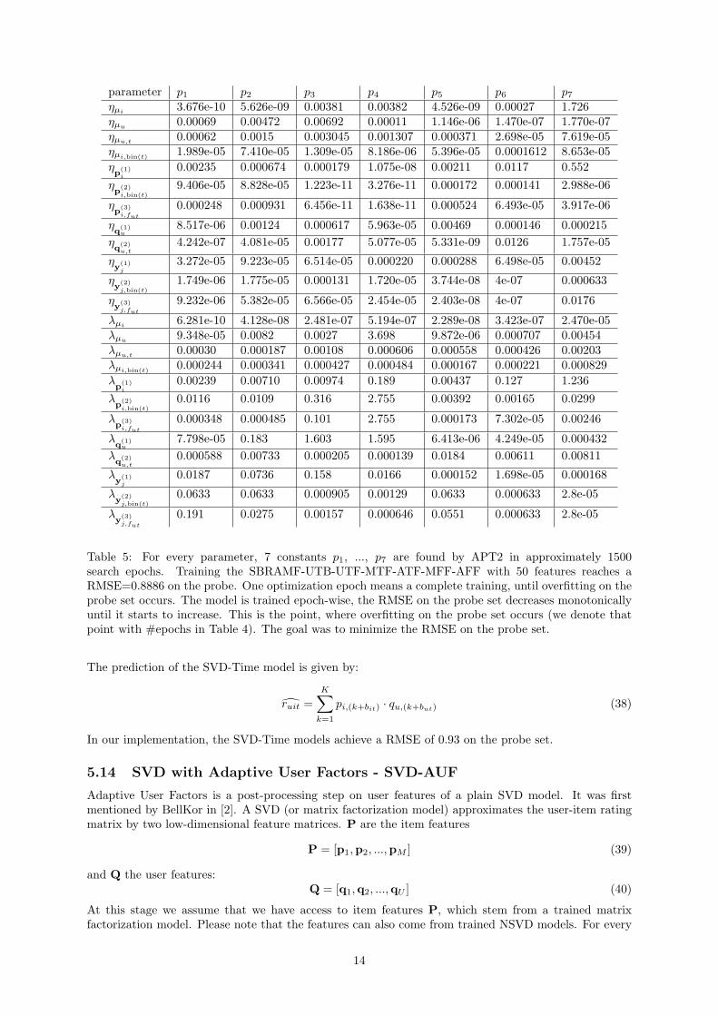
parameter p1 p2 p3 p4 p5 p6 p7

ηµi3.676e-10 5.626e-09 0.00381 0.00382 4.526e-09 0.00027 1.726

ηµu0.00069 0.00472 0.00692 0.00011 1.146e-06 1.470e-07 1.770e-07

ηµu,t 0.00062 0.0015 0.003045 0.001307 0.000371 2.698e-05 7.619e-05ηµi,bin(t) 1.989e-05 7.410e-05 1.309e-05 8.186e-06 5.396e-05 0.0001612 8.653e-05ηp

(1)i

0.00235 0.000674 0.000179 1.075e-08 0.00211 0.0117 0.552ηp

(2)i,bin(t)

9.406e-05 8.828e-05 1.223e-11 3.276e-11 0.000172 0.000141 2.988e-06

ηp

(3)i,fut

0.000248 0.000931 6.456e-11 1.638e-11 0.000524 6.493e-05 3.917e-06

ηq

(1)u

8.517e-06 0.00124 0.000617 5.963e-05 0.00469 0.000146 0.000215ηq

(2)u,t

4.242e-07 4.081e-05 0.00177 5.077e-05 5.331e-09 0.0126 1.757e-05

ηy

(1)j

3.272e-05 9.223e-05 6.514e-05 0.000220 0.000288 6.498e-05 0.00452

ηy

(2)j,bin(t)

1.749e-06 1.775e-05 0.000131 1.720e-05 3.744e-08 4e-07 0.000633

ηy

(3)j,fut

9.232e-06 5.382e-05 6.566e-05 2.454e-05 2.403e-08 4e-07 0.0176

λµi6.281e-10 4.128e-08 2.481e-07 5.194e-07 2.289e-08 3.423e-07 2.470e-05

λµu 9.348e-05 0.0082 0.0027 3.698 9.872e-06 0.000707 0.00454λµu,t

0.00030 0.000187 0.00108 0.000606 0.000558 0.000426 0.00203λµi,bin(t) 0.000244 0.000341 0.000427 0.000484 0.000167 0.000221 0.000829λp

(1)i

0.00239 0.00710 0.00974 0.189 0.00437 0.127 1.236λp

(2)i,bin(t)

0.0116 0.0109 0.316 2.755 0.00392 0.00165 0.0299

λp

(3)i,fut

0.000348 0.000485 0.101 2.755 0.000173 7.302e-05 0.00246

λq

(1)u

7.798e-05 0.183 1.603 1.595 6.413e-06 4.249e-05 0.000432λq

(2)u,t

0.000588 0.00733 0.000205 0.000139 0.0184 0.00611 0.00811

λy

(1)j

0.0187 0.0736 0.158 0.0166 0.000152 1.698e-05 0.000168

λy

(2)j,bin(t)

0.0633 0.0633 0.000905 0.00129 0.0633 0.000633 2.8e-05

λy

(3)j,fut

0.191 0.0275 0.00157 0.000646 0.0551 0.000633 2.8e-05

Table 5: For every parameter, 7 constants p1, ..., p7 are found by APT2 in approximately 1500search epochs. Training the SBRAMF-UTB-UTF-MTF-ATF-MFF-AFF with 50 features reaches aRMSE=0.8886 on the probe. One optimization epoch means a complete training, until overfitting on theprobe set occurs. The model is trained epoch-wise, the RMSE on the probe set decreases monotonicallyuntil it starts to increase. This is the point, where overfitting on the probe set occurs (we denote thatpoint with #epochs in Table 4). The goal was to minimize the RMSE on the probe set.

The prediction of the SVD-Time model is given by:

ruit =K∑k=1

pi,(k+bit) · qu,(k+but) (38)

In our implementation, the SVD-Time models achieve a RMSE of 0.93 on the probe set.

5.14 SVD with Adaptive User Factors - SVD-AUF

Adaptive User Factors is a post-processing step on user features of a plain SVD model. It was firstmentioned by BellKor in [2]. A SVD (or matrix factorization model) approximates the user-item ratingmatrix by two low-dimensional feature matrices. P are the item features

P = [p1,p2, ...,pM ] (39)

and Q the user features:Q = [q1,q2, ...,qU ] (40)

At this stage we assume that we have access to item features P, which stem from a trained matrixfactorization model. Please note that the features can also come from trained NSVD models. For every

14

single prediction ruirui = pTi qu (41)

we recompute the user feature in the following way

qu = SolveLinearEquationSystem(A,b). (42)

The matrix A has |R(u)| rows and K columns, where K is the number of features. The target vector bconsists ratings from user u. Each element in the matrix A = ajk is given by

ajk = pjk · sim(i, j) (43)

The pjk are values from the K-dimensional item feature pj . In Equation 42 we use two different linearequation solvers. We call the first one “PINV”, which is a standard solver from the LAPACK softwarepackage. The second one is the nonnegative solver from [2]. The ridge regression constant in the numericsolvers is denoted by λ. Exact values for λ and the kind of solver are reported for every predictor inAppendix A. In Table 6 we list the similarity measures, which were used in the SVD-AUF

similarity measure sim(i, j)DateSim κ+ (|tui − tuj |+ γ)−β

SupportSim κ+ |(|R(i)| − |R(j)|)|−βProductionYearSim κ+ |yeari − yearj |−βPearsonSim κ+ σ(δ · cij + γ)

Table 6: SVD-AUF: These similarity measures are used for the SVD with adaptive user factors. The cijis a shrunken Pearson correlation as in Equation 1. σ(x) is the sigmoid function from Equation 3.

The similarity measure and all meta parameters from Table 6 are reported for every results in thepredictor list (Appendix A).

5.14.1 SVD-AUF with Kernel Ridge Regression

An extention to the SVD-AUF algorithm is the use Kernel Ridge Regression (see [9] for details). KRRlearns a model from the input features A and targets b, as sketched in Algorithm 2. Standard linearregression needs dot products of input dimensions (columns of feature matrix A), kernel ridge regressionrelies on kernel dot product of input features (rows of feature matrix A). This forms the Gram matrixK. If a linear kernel is used, KRR is equivalent to linear regression.

As stated in the SVD-AUF, a trained matrix factorization model, especially the item features P (seeEquation 39) must be available. We train a KRR model Ωu(x) for each user u. Features and targets areequal to the from Equation 42. The KRR is able to predict a rating for any given item feature pi

rui = Ωu(pi) (44)

The kernels which were used in SVD-AUF with Kernel Ridge Regression are listed in Table 7.

Input: Data matrix A, targets b, new test feature xOutput: The prediction model Ω(x)Tunable: Ridge regression constant λ, kernel hyperparametersK = kdot(A,AT ), where k(xi,xj) is the kernelized dot product1

W = (K + λI)−1b2

Ω(x) = kdot(x,AT ) ·W3

Algorithm 2: The KRR - “kernel ridge regression” learn algorithm

In Algorithm 2 the steps required to train the KRR algorithm can be seen. The computational andmemory intensive step is to invert the Gram matrix (K + λI)−1, which has a time complexity of O(N3).This limits the number of N training samples, so we are skipping ratings from users with too many votes.In this case, the ratings of user u are sorted according to their movie support. Afterwards we limit thenumber of ratings per user to 1000.

15

kernel k(xi,xj)polynomial (α+ xiTxj)β

pow κ(α+xiT xj)β

extended polynomial |γ(α+ xiTxj)|β

Table 7: SVD-AUF: These kernels are used in KRR postprocessing.

5.15 SVD Trained with Alternating Least Squares - SVD-ALS

The SVD-ALS idea was described in [4]. For the SVD model, training of item and user features are doneby applying a linear equation solver on item side, while the user features are kept constant. Afterwardsthe user features are updated with constant item features. The training stops, when the features do notchange any more. SVD-ALS has the advantage that no learning rate is required. A regularization forthe solver is still required. We use a standard linear equation solver as described in Section 6.1. RMSEvalues on the probe set are slightly worse compared to a SVD with stochastic gradient descent. Our bestmodels achieve a probe RMSE in the region of 0.91.

5.16 Rating Matrix Factorization - SVD

This is a plain SVD with no user and movie biases. The training is done with stochastic gradient descentover a randomized training list of samples L = (u1, i1), . . . , (uL, iL). Details can be found in [17]. Aprediction is given by

rui = piTqu (45)

Large SVD models achieve a RMSE of 0.905 on the probe set.

5.17 Neighborhood Aware Matrix Factorization - NAMF

This model combines matrix factorization with neighborhood information and is fully described in [17]and [18]. For tuning the involved parameters, we use APT1. This method stayed unchanged since theProgress Prize 2008.

5.18 Regression on Similarity - ROS

Factorization of the item-item or user-user correlation is described in [18]. This method has not changedsince the Progress Prize 2008.

6 Probe Blending

Since the progress prize 2008 we made major progress on the probe blending side. Blending a set ofpredictors is a standard regression problem. The list of methods for regression problems is very long, butdue to the 1408395 probe samples, not every method can be used. In the beginning of the competitionwe used linear regression. For the progress prize 2008 we additionally used neural networks. It turnedout that the results can be additionally improved by using ensemble of probe blends.

The Netflix prize showed that a very diverse ensemble of CF algorithms yields great results. We usedthe same idea for the blending. So we used diverse methods on diverse sets of predictors. In the followingwe describe all regression methods, additional features and predictor subsets.

6.1 Linear Regression - LinearBlend

Linear Regression is a standard tool and yields good results. The big advantage of pure linear regressionis clearly the speed. We use a L2 regularization to control overfitting with the regularization constantλ. A standard least square solver (LAPACK) is used. The time complexity is nm2, with n being thenumber of equations and m the number of predictors (features). The space complexity is m2. Sometimeswe restrict the linear equation solver to nonnegative weights. In these cases we use the iterative solveras described in [3].

16

6.2 Polynomial Regression - PolyRegressionBlend

As an extension to linear regression, we add higher order terms to capture non-linear properties of thepredictors. Polynomial regression simply extends the predictor set with higher order terms X ·w0 + X2 ·w1 + X3 ·w2 + .... Order 2 means that we extend the set with quadratic duplicates.

6.3 Binned Linear Regression

The idea of binned linear regression is to divide the probe set into disjoint subsets, called bins in thefollowing, and fit a different set of blending weights to every bin. We choose the boundaries in order tohave equal sized bins (equal number of ratings) and to prevent the number of bins from getting too largeto avoid overfitting each bin.

6.3.1 Support Based Bins - N-SupportBins

We define the support sui as the minimum of the ratings by user u and item i.

sui = min(|N(u)|, |N(i)|) (46)

Based on this support, we split the probe set into bins. The motivation behind these splits is thatsome algorithms work better on users with few ratings, while others give great results when there isenough information available. These split criteria work best (compared with date and frequency).

6.3.2 Date Based Bins - N-DateBins

Another way to split the probe set is to base the bins on the rating date. The results are slightly worse,compared to the support based splits.

6.3.3 Frequency Based Bins - N-FrequencyBins

Here the probe set is binned based on the number of ratings a user has given per day. Results are slightlyworse compared to the support based splits.

6.3.4 Clustering Based Bins - N-ClusterBins

Every result from the exact residual framework (see Section 3.3) delivers a k-fold cross-validation pre-diction of the training set. This has the property that strong models cannot overfit the training set,which has a positive effect on the quality of the clusters. Initially, each user and item is assigned to Mitem and N user clusters c(m)

i and c(n)u . The first step is to calculate linear regression blending weights

per cluster. The second step is to move each item i and each user u to the cluster, where the trainingRMSE lowers best. So assignments to clusters were changed by a greedy schema. This is repeated 100times, the cluster assignment stabilizes very fast. The final clusters c(m)

i and c(n)u were used to calculate

a binned linear regression on the probe set, this means we calculate a separate linear regression for eachcluster.

6.4 Subset Generation

Not all blends got trained on all available predictors. This has two main reasons. The most important is,to introduce diversity in the ensemble of blends. The other reason is that it reduces the computationalcomplexity of the individual blends.

6.4.1 Forward Selection

The goal is to select K predictors, which give good blending results. We start with the best singlepredictor and iteratively add the predictor which improves the blending RMSE best. Obviously thisgreedy method does not guarantee to find the optimal subset of predictors.

17

6.4.2 Backward Selection

The goal is the same as for the forward selection. This time we start with a linear blend, including allavailable predictors, and iteratively deselect the predictor which contributes the least. The deselectionprocess is stopped, if there are only K predictors left. As for the forward selection, there is no guaranteeto find the optimal subset.

6.4.3 Probe-Quiz Difference Selection - PQDiff

The typical predictor has a lower RMSE on the quiz set than on the probe set. We call it probe-quizdifference. This difference comes from the retraining. For the quiz set predictions the algorithms areretrained on the complete available data, including the probe data. So there is more training dataavailable for the quiz predictions. This is why these predictions get more accurate. This probe-quizdifference differs between the algorithms.

The idea is now, to group the predictors by the probe-quiz difference.

6.5 Neural Network Blending - NNBlend

A neural network is a function approximator from a P -dimensional input space to the output space.It is trained by stochastic gradient descent by applying the backprop algorithm. P is the numberof predictions used for blending. The output is a scalar, representing the predicted value. We havea detailed description of the setup in BigChaos Progress Prize 2008 report [17]. This is part of ourmost successful blending schema, in terms of minimizing the RMSE on the quiz. All NNBlends uselog(|R(u)|+ 1) and log(|R(i)|+ 1) as additional inputs. The initial learning rate is η = 0.0005 and everyepoch we subtracted η(−). We report η(−), the number of epochs where the training stops, number ofhidden layers and the neuron configuration. For standard NNBlends we use η(−) = 3e− 7 and train for1334 epochs. During ongoing improvement of the blending technique we use k-fold cross validation tooptimize the net configuration, apply 2 hidden layers and break the training when the RMSE on thevalidation set is minimal.

6.6 Ensemble Neural Network Blending - ENNBlend

Sampling the P -dimensional predictor space can help to model interactions between single predictors.The blending schema selects k random predictors from P in total and blend them with a small neuralnet (NNBlend). This results in N predictions, which are again blended by a binned blender. Pleasenote that every NNBlend itself adds two additional support inputs (see 6.5). Good values are k = 4,N = 1200 and a linear blend on 4-FrequencyBins. The ENNBlend reaches the best quiz RMSE withprobe blending.

6.7 Bagged Gradient Boosted Decision Tree - BGBDT

BGBDT combines the idea of Gradient Boosted Decision Trees, as described by Friedman[7],[8], withthe bagging and random subspace idea of Random Forests [6]. The splits are simple axis parallel ones.Random Forests use a random subspace idea, which is also used here. At each split point, we select Srandom features, calculate optimal splitpoints for every selected feature and use the split, which reducesthe RMSE best. Every tree is grown to the maximum tree depth d. The splitting is also stopped, ifa leaf node has less than Nmin datapoints. So in difference to Random Forests, the trees are not fullygrown.

The basic idea of gradient boosting is to successively train trees on the residuals of the previous ones.The learning rate λ controls the contribution of a individual tree and Nboost stands for the number oftrees in a single boosting chain. We additionally use a bagging idea. Nbag stands for the bagging size(the number of boosting chains, which are trained simultaneously). Each bagging set of training ratingsis drawn with replacement from the originals and has the same size. The structure of a BGBDT can beseen in Figure 5, and the general training’s procedure is described in Algorithm 3.

18

Nboost

Nbag

Gradient Boosting

Figure 5: This figure shows the structure of a BGBDT. Each cell represents a simple decision tree.The tree on the left trains on the raw data. The second tree trains on the residual error of the first;the third tree on the residuals of the second and so on. Thus a colored row forms a chain of gradientboosted decision trees. Each colored row represents different training examples, which are drawn withreplacement from the original training samples (bagging). So we train multiple chains of gradient boosteddecision trees in parallel, whereas each chain uses its own training set.

Input: A matrix P with probe predictions, and a vector with target ratings r.for i = 1 to Nbag do1

Draw Pi with replacement from P, while ri should contain the corresponding target ratings.2

end3

RMSEbest =∞4

RMSEepoch = 10005

j = 06

while RMSEepoch ≤ RMSEbest and j < Nboost do7

for i = 1 to Nbag do8

Tij = TrainSingleTree(Pi, ri, Nmin, S); trains the tree Tij9

ri = ri − λ ·GenerateSingleTreePrediction(Tij ,Pi); calculate the residuals10

end11

Calculate the RMSEepoch.12

if RMSEepoch ≤ RMSEbest then13

RMSEbest = RMSEepoch14

end15

j = j + 116

end17

Algorithm 3: The training of a BGBDT.

As additional input features we always use the number of user votes, movie votes and the rating date.A very nice property of this sort of tree is that there is no need for a rescaling or any sort of monotonictransformation (e.g. logarithm) of the features as needed for neural networks.

Experiments show that these parameters are very insensitive. Good parameters are λ = 0.1, Nboost =250, Nbag = 32, d = 12, Nmin = 100, S = 10. The exact parameters used for the blendings can be foundin the predictors list in Appendix A.5. The RMSEs of the BGBDT blends are not as good as for neuralnetworks, but they do very well in the final quiz blend.

6.8 KRR on a Probe Subset - KRRBlend

We use linear, binned linear regression, non linear blending methods like NNBlend and BGBDT. Kernelregression methods are very hard to apply on the blending problem because of the huge size of the probeset. To make Kernel Ridge Regression work, we use a subset of the probe set as training set for the

19

KRR. Size of 4000 is a good compromise between training/prediction speed and accuracy. The algorithmwe use for blending is exact the same as in Algorithm 2 from Section 5.14.1. For all blending results, aGauss kernel was used.

6.9 SVD Feature Predictor Extraction

The goal of predictor feature extraction is to generate a probe/qualifying pair from latent features of acollaborative filtering model. A matrix factorization model learns features from the data with stochasticgradient descent. Users and items have their latent factors, which describe their property. These featurescan be used to extend the blend. We use our most accurate SVD model to produce predictions, whichwe integrate in various blends. Recall the prediction formula from the SBRAMF-UTB-UTF-MTF-ATF-MFF-AFF model ruit =

µi+µu+µu,t+µi,bin(t)+(p(1)i + p(2)


)T q(1)u + q(2)

u,t +

asymmetric part︷︸︸︷1√|N(u)|

∑j∈N(u)

(y(1)j + y(2)

j,bin(t) + y(3)j,fut

).

This model has 4 biases (2 item biases, 2 user biases), 6 item dependent features (3 item, 3 asymmetric)and 2 user dependent features. The asymmetric part of the model is an additional user feature. Forevery (u, i) in the probe and qualifying set we extract 4+k · (6+2+1) predictors, where k is the numberof features. As an extension, we add all possible dot products between item and user features. Thisresults in 50 additional predictors, which we denote with -cross- in the probe blending Section 6.

6.10 RBM Feature Predictor Extraction

In its essence a RBM calculates a low dimensional representation of the visible units. This property canbe used to calculate user and movie features. These features are great additional inputs for the nonlinearprobe blends. A user is represented as a bag of movies on the visible layer of the RBM, on the hiddenlayer you get a low dimensional representation of the user. The same can be done with movies, in orderto get a low dimensional movie representation. For the blending features we use less hidden units as wewould use for pure CF. In most blends we use a user and movie representation with 20 features (hiddenunits). In the predictor list, we clearly state, which predictor uses RBM user/movie features.

6.11 KNN Predictor Extraction

The prediction in an item-item KNN is a weighted sum of ratings from k-best neighbors. We extractpredictors from the k-best neighbors in the following format:

index user item k = 1, item j (1st neighbor) k = 2, item j (2nd neighbor)1 u i cij · ruj cij log(sij + 1) ruj exp(−|tuj − tui|/500) ...2 ...

Table 8: KNN predictor extraction

Index is the number of samples in the probe or the qualifying set. cij is the shrunken Pearsoncorrelation between two items i and j. Shrinkage is set to 200. sij is the support, the number of commonusers of item i and j. rij is the known rating from user u on item j. As listed in Table 8, five values areextracted for every neighbor item j, when k = 50 we extract 250 additional predictions.

7 Quiz Blending

The whole ensemble of predictors from BellKor’s Pragmatic Chaos is blended linearly in the end. Theensemble of predictors includes the individual predictors and the predictors obtained from nonlinearprobe blends as described in Section 6.

7.1 Linear Blending on the Quiz Data Set without the Quiz Ratings

For the quiz data set of size N , let y ∈ RN be the unobserved vector of true ratings and x1, ...,xp ∈ RNbe p vectors of known predictions. Let X be the N -by-p matrix with columns x1, ...,xp For simplicity,

20

and to clarify the impact of selected approximations that follow, assume that the mean 1 has been sub-tracted from y and from each column of X.

Our goal is to find the linear combination of x1, ...,xp that best predicts y. If y was known, we woulduse linear regression. That is, we would estimate y by Xβ where

β =(XTX

)−1 (XTy

)(47)

Note that there is no guarantee that the elements of β will all be non negative or that they will sumto 1.

While it is easy to compute(XTX

)−1 (for the full qualifying data set), the missing link is the p-by-1vector

(XTy

). Fortunately, it is possible to estimate each component of this vector with high precision.

Consider the j-th element: ∑u

xjuyu. (48)

Simple algebra implies that the above expression can be rewritten as

12

[∑u

y2u +

∑u

x2ju −

∑u

(yu − xju)2

](49)

Because all predictors are centered, the first term inside the brackets can be closely approximated byN times the quiz set variance, which is known to be 1.274. The second term can be computed exactly(for the full qualifying data). The last term is simply N times the MSE (RMSE2) associated with xjfor the Quiz data 2. It is guaranteed to be accurate within about 0.01 percent. Although the constantN is unknown, it cancels out in the formula for β.

However, the final accuracy of β may be much less if the estimators are highly correlated. Thus, we usedridge regression, as follows:

β =(XTX + λNI

)−1 (XTy

)(50)

We used λ = 0.0014 (in contrast to 0.0010 for the 2008 progress prize).

We are also able to estimate the RMSE for the resulting composite estimator. For λ = 0, the MSEis simply 1.274−Var(Xβ), where Var(Xβ) is the variance of the linear blend.

For λ > 0, the calculation is slightly more complicated:

MSE(Xβ) =∑i

βi (MSE(xi)−Var(xi)) + 1.274

(1−

∑i

βi

)+ Var(Xβ) (51)

7.2 Estimated Degree of Over Fitting the Quiz Set Relative to the Test Set

As just noted, our final prediction set was a linear combination of prediction sets based on an approxima-tion of ridge regression of ratings on many individual prediction sets for the quiz data. While ordinaryleast squares regression would minimize the RMSE for the quiz data among all linear combinations, ourgoal was to minimize RMSE for the test data. It is well known that regression can over fit to trainingdata (the quiz data) leading to poor performance for new data (the test data). Consequently, it was im-portant to understand the extent to which improvement on the quiz RMSE over estimated improvementon the test RMSE.

For ordinary least squares regression, the “bias” of the quiz MSE (MSEq) as an estimate of the testMSE (MSEt) is −2p/N , where p is the number of prediction sets and N is the size of the quiz data (see

1The Quiz mean is known to be 3.674, while its variance is 1.274see: www.netflixprize.com/community/viewtopic.php?id=503

2Because we get the RMSE for the Quiz data, there is some danger of overfitting the Quiz data, leading to poorerpredictions for the test data. That danger is greatest if p is large and the xj are highly correlated with each other.

21

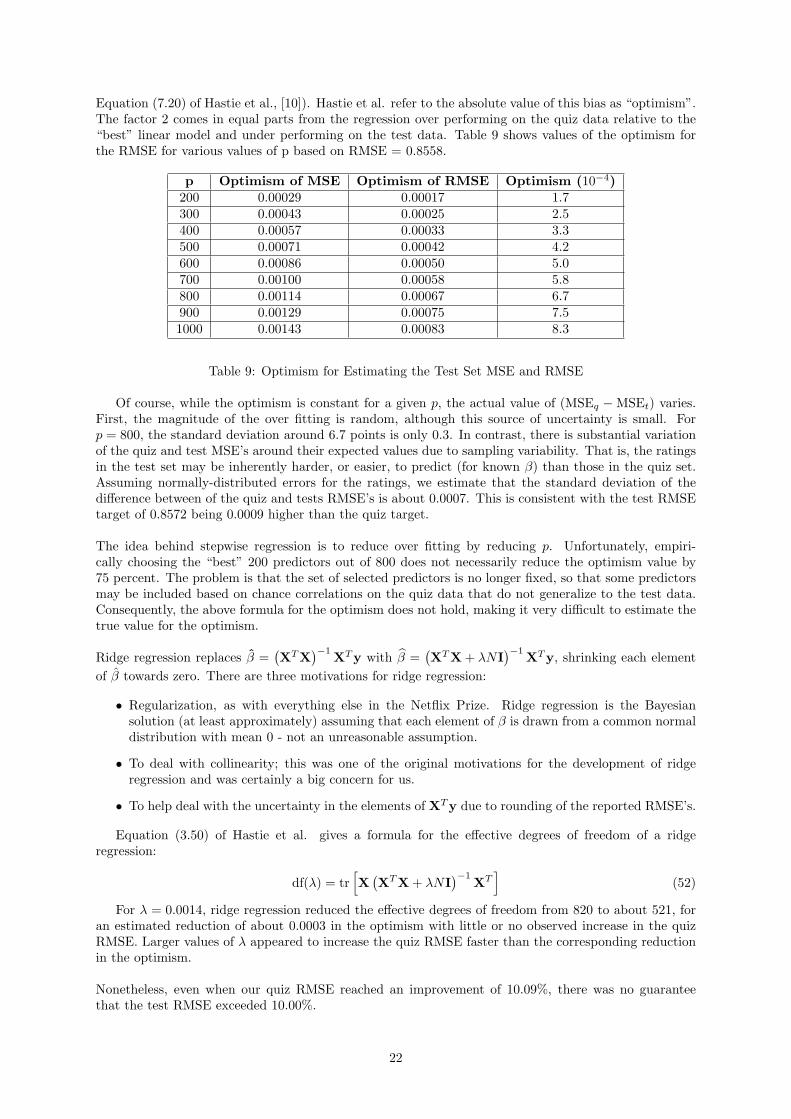
Equation (7.20) of Hastie et al., [10]). Hastie et al. refer to the absolute value of this bias as “optimism”.The factor 2 comes in equal parts from the regression over performing on the quiz data relative to the“best” linear model and under performing on the test data. Table 9 shows values of the optimism forthe RMSE for various values of p based on RMSE = 0.8558.

p Optimism of MSE Optimism of RMSE Optimism (10−4)200 0.00029 0.00017 1.7300 0.00043 0.00025 2.5400 0.00057 0.00033 3.3500 0.00071 0.00042 4.2600 0.00086 0.00050 5.0700 0.00100 0.00058 5.8800 0.00114 0.00067 6.7900 0.00129 0.00075 7.51000 0.00143 0.00083 8.3

Table 9: Optimism for Estimating the Test Set MSE and RMSE

Of course, while the optimism is constant for a given p, the actual value of (MSEq −MSEt) varies.First, the magnitude of the over fitting is random, although this source of uncertainty is small. Forp = 800, the standard deviation around 6.7 points is only 0.3. In contrast, there is substantial variationof the quiz and test MSE’s around their expected values due to sampling variability. That is, the ratingsin the test set may be inherently harder, or easier, to predict (for known β) than those in the quiz set.Assuming normally-distributed errors for the ratings, we estimate that the standard deviation of thedifference between of the quiz and tests RMSE’s is about 0.0007. This is consistent with the test RMSEtarget of 0.8572 being 0.0009 higher than the quiz target.

The idea behind stepwise regression is to reduce over fitting by reducing p. Unfortunately, empiri-cally choosing the “best” 200 predictors out of 800 does not necessarily reduce the optimism value by75 percent. The problem is that the set of selected predictors is no longer fixed, so that some predictorsmay be included based on chance correlations on the quiz data that do not generalize to the test data.Consequently, the above formula for the optimism does not hold, making it very difficult to estimate thetrue value for the optimism.

Ridge regression replaces β =(XTX

)−1XTy with β =

(XTX + λNI

)−1XTy, shrinking each element

of β towards zero. There are three motivations for ridge regression:

• Regularization, as with everything else in the Netflix Prize. Ridge regression is the Bayesiansolution (at least approximately) assuming that each element of β is drawn from a common normaldistribution with mean 0 - not an unreasonable assumption.

• To deal with collinearity; this was one of the original motivations for the development of ridgeregression and was certainly a big concern for us.

• To help deal with the uncertainty in the elements of XTy due to rounding of the reported RMSE’s.

Equation (3.50) of Hastie et al. gives a formula for the effective degrees of freedom of a ridgeregression:

df(λ) = tr[X(XTX + λNI

)−1XT]

(52)

For λ = 0.0014, ridge regression reduced the effective degrees of freedom from 820 to about 521, foran estimated reduction of about 0.0003 in the optimism with little or no observed increase in the quizRMSE. Larger values of λ appeared to increase the quiz RMSE faster than the corresponding reductionin the optimism.

Nonetheless, even when our quiz RMSE reached an improvement of 10.09%, there was no guaranteethat the test RMSE exceeded 10.00%.

22

8 Discussion

During the nearly 3 years of the Netflix competition, there were two main factors which improved theoverall accuracy: The quality of the individual algorithms and the ensemble idea.

On the algorithmic side there was a strong focus on matrix factorization techniques. The big advan-tage of these methods is, that they can be trained efficiently and predictions can be generated quickly.Additionally, the integration of additional signals and views on the data is easy. So the simple matrixfactorization has grown to a big integrated model, which delivers outstanding performance. The compe-tition was not only about matrix factorization, RBMs were successfully shown to yield great results forcollaborative filtering. Especially if RBMs are combined with KNN models. The integration of additionalsignals, such as time is not that easy.

Over the 3 years of the competition, a lot of effects were found in the data. During the first year thebiggest discovery was the binary information, accounting for the fact that people do not select movies forrating at random. In the second year there was a focus on temporal effects. Small long term effects andstronger short term effects, especially the one day effect, was very strong [14]. It is hard to say whetherthis effect is grounded in multiple users sharing the same account, or the changing mood of a person.

The other main driving force in the competition was the ensemble idea. The ensemble idea was partof the competition from the beginning and evolved over time. In the beginning, we used different modelswith different parametrization and a linear blending. The models were trained individually and the metaparameters got optimized to reduce the RMSE of the individual model. The linear blend was replacedby a nonlinear one, a neural network. This was basically the solution for the progress prize 2008, aensemble of independently trained and tuned predictors, and a neural network for the blending. In fall2008, we realized that training and optimizing the predictors individually is not optimal. Best blendingresults are achieved when the whole ensemble has the right tradeoff between diversity and accuracy. Sowe started to train the predictors sequentially and stopped the training when the blending improvementwas best. Also the meta parameters were tuned, to achieve best blending performance. The next stepin the evolution of the ensemble idea was to replace the single neural network blend by an ensemble ofblends. In order to maximize diversity within the blending ensemble, the blends used different subsetsof predictors and different blending methods. Figure 6 shows the RMSE improvements compared to thenumber of predictors. Within the first predictors there are a lot of different blends (the first 18 are listedin Appendix C). This clearly shows that the diverse set of nonlinear probe blends is an important partof our solution.

The Netflix prize boosted the collaborative filtering research, because it enabled direct comparison ofresults and encouraged an open discussion of ideas in the forum and on conferences. It would be greatto see similar competitions in future.

References

[1] Netflix Prize homepage. Website, 2006. http://www.netflixprize.com.

[2] R. Bell and Y. Koren. Scalable collaborative filtering with jointly derived neighborhood interpolationweights. In IEEE International Conference on Data Mining. KDD-Cup07, 2007.

[3] R. Bell, Y. Koren, and C. Volinsky. Modeling relationships at multiple scales to improve accuracyof large recommender systems. In KDD ’07: Proceedings of the 13th ACM SIGKDD internationalconference on Knowledge discovery and data mining, pages 95–104, New York, NY, USA, 2007.ACM.

[4] R. M. Bell, Y. Koren, and C. Volinsky. The BellKor solution to the Netflix Prize, October 2007.

[5] R. M. Bell, Y. Koren, and C. Volinsky. The BellKor 2008 solution to the Netflix Prize, October2008.

[6] L. Breiman. Random forests. Machine Learning, 45:5–32, 2001.

[7] J. Friedman. Greedy function approximation: A gradient boosting machine. Technical report,Salford Systems, 1999.

[8] J. Friedman. Stochastic gradient boosting. Computational Statistics & Data Analysis, 2002.

23

100

101

102

103

0.855

0.8555

0.856

0.8565

0.857

0.8575

0.858

0.8585

#predictors

quiz

RM

SE

blend RMSEGrand Prize

Figure 6: How many results are really needed? With 18 results we breach the 10% (RMSE 0.8563)barrier. Within these results there are 11 nonlinear probe blends and 7 unblended predictors. Anordered list of these predictors can be found in Appendix C.

[9] I. Guyon. Kernel Ridge Regression tutorial, accessed Aug 31, 2009. http://clopinet.com/isabelle/Projects/ETH/KernelRidge.pdf.

[10] T. Hastie, R. Tibshirani, and J. Friedman. The Elements of Statistical Learning. Springer, 1st

edition, 2001.

[11] Y. Koren. Factorization meets the neighborhood: a multifaceted collaborative filtering model. InKDD ’08: Proceeding of the 14th ACM SIGKDD international conference on Knowledge discoveryand data mining, pages 426–434, New York, NY, USA, 2008. ACM.

[12] Y. Koren. The BellKor solution to the Netflix Grand Prize, 2009.

[13] A. Paterek. Improving regularized singular value decomposition for collaborative filtering. Proceed-ings of KDD Cup and Workshop, 2007.

[14] G. Potter. Putting the collaborator back into collaborative filtering. In KDD Workshop at SIGKDD08, August 2008.

[15] R. Salakhutdinov, A. Mnih, and G. E. Hinton. Restricted boltzmann machines for collaborativefiltering. In ICML, pages 791–798, 2007.

[16] G. Takacs, I. Pilaszy, B. Nemeth, and D. Tikk. Matrix factorization and neighbor based algo-rithms for the netflix prize problem. In RecSys ’08: Proceedings of the 2008 ACM conference onRecommender systems, pages 267–274, New York, NY, USA, 2008. ACM.

[17] A. Toscher and M. Jahrer. The BigChaos solution to the Netflix Prize 2008. Technical report,commendo research & consulting, October 2008.

[18] A. Toscher, M. Jahrer, and R. Legenstein. Improved neighborhood-based algorithms for large-scalerecommender systems. In KDD Workshop at SIGKDD 08, August 2008.

24

[19] M. Wu. Collaborative filtering via ensembles of matrix factorizations. Proceedings of KDD Cup andWorkshop, 2007.

25

A Predictor List

This section lists all results produced by team BigChaos and blends of results by Pragmatic Theory andBellKor. All listed results are quiz RMSEs.

A.1 BigChaos Progress Prize 2008 Results: PP-*

60 predictors were taken from the BigChaos Progress Prize 2008 report, the rest was dropped. Thereference number and the algorithm in brackets is the one, which is listed in [17].

PP-01 rmse=0.9028Corresponds to 3. (BasicSVD)






PP-07 rmse=0.9592Corresponds to 10. (SVD-AUF)

PP-08 rmse=0.9038Corresponds to 11. (SVD-ALS)

PP-09 rmse=0.9842Corresponds to 12. (TimeSVD)




PP-13 rmse=0.8981Corresponds to 18. (NAMF)

PP-14 rmse=0.9070Corresponds to 26. (RBMV5)



26








PP-24 rmse=0.9229Corresponds to 38. (KNN-BASIC)

PP-25 rmse=0.9013Corresponds to 39. (KNN-BASIC)

PP-26 rmse=0.9151Corresponds to 41. (KNNMovieV7)


PP-28 rmse=0.8942Corresponds to 43. (KNNMovie)








PP-36 rmse=0.8900

27

Corresponds to 51. (KNNMovieV3)






PP-42 rmse=0.9300Corresponds to 62. (ROS)




PP-46 rmse=0.9366Corresponds to 69. (AFM)

PP-47 rmse=0.885Corresponds to 74. (GTE)







PP-54 rmse=0.8872Corresponds to 82. (CTD)


28



PP-58 rmse=0.8845Corresponds to 86. (MTD)

PP-59 rmse=0.913Corresponds to 89. (NN)

PP-60 rmse=0.9178Corresponds to 91. (NN)

A.2 Optimize the Predictors Individually on the Probe Set: OP-*

These predictors got trained in the same way, as for the progress prize 2008. They are trained andoptimized individually in order to minimize the probe set RMSE.

A.2.1 Basic SVD

OP-01 rmse=0.9108BasicSVD, Residual: 1GE, k=64, η = 0.001, λ = 0.019, α = 2.0

OP-02 rmse=0.9126BasicSVD, Residual: 14GE, k=100, η = 0.002, λ = 0.01, α = 2.0

OP-03 rmse=0.9066BasicSVD, Residual: OP-18, k=300, η = 0.001, λ = 0.007, α = 2.0

OP-04 rmse=0.9177BasicSVD, Residual: no, force non-negative weights, k=100, η = 0.0005, λ = 0.003, α = 2.0

A.2.2 Neighborhood Aware Matrix Factorization

OP-05 rmse=0.8993NAMF, Residual: 1GE, k=300, η = 0.004, λ = 0.02, bestCorr = 50 [Pearson on 10GE]

OP-06 rmse=0.8856NAMF, Residual: 1GE, k=100, η = 0.002, λ = 0.02, bestCorr = 50 [Pearson on 10GE], For this predic-tor we inserted a predicted qualifying set (RMSE of 0.8736) into the training ratings.

A.2.3 RBMV6

OP-07 rmse=0.9270RBMV6, Residual: 10GE, 50 hidden units, η = 0.002, λ = 0.00035

29

A.2.4 Movie KNN

OP-08 rmse=0.9154KNNMovieV3, Residual: 10GE, k=48, Pearson correlation, α = 600, β = 540, γ = −2.38, δ = 10.8

OP-09 rmse=0.8987KNNMovieV3, Residual: PP-46, k=34, Pearson correlation, α = 292, β = 787, γ = −2.47, δ = 7.8

OP-10 rmse=0.8973KNNMovie, Residual: BasicSVD 300 dim, k=80, Pearson correlation

OP-11 rmse=0.8851KNNMovieV3, Residual: blended RBMV3, k=55, Pearson correlation, α = 842, β = 540, γ = −2.43,δ = 12.7

A.2.5 Regression on Similarity

OP-12 rmse=0.936ROS factorized, Residual: 6 GE, on movie-side, k=20, η=3.5e-3, λ=1e-3

OP-13 rmse=0.9241ROS, unfactorized, Residual: 10 GE, η=1, λ =1e-4

A.2.6 Global Time Effects

OP-14 rmse=0.9545GTE, Residual: no, 8 effects

OP-15 rmse=0.8884GTE, Residual: PP-34, 1 effects

A.2.7 Customer Time Dep Model

OP-16 rmse=1.0429CTD, Residual: OP-18, Linear Weight, α = 35, β = 23, γ = 122

OP-17 rmse=0.898CTD, Residual: BasicSVD 300 dim, Near Gaussian Weight, α = 5693, β = 7, γ = 21

OP-18 rmse=1.0476CTD, Residual: no, Near Gaussian Weight, α = 15, β = 5, γ = 0.55

OP-19 rmse=0.9537CTD, Residual: 10 GE, Near Gaussian Weight, α = 10400, β = 8, γ = 0.49

A.2.8 Movie Time Dep Model

OP-20 rmse=0.9514MTD, Residual: OP-19, Near Gaussian Weight, α = 0.15, β = 85, γ = 16

30

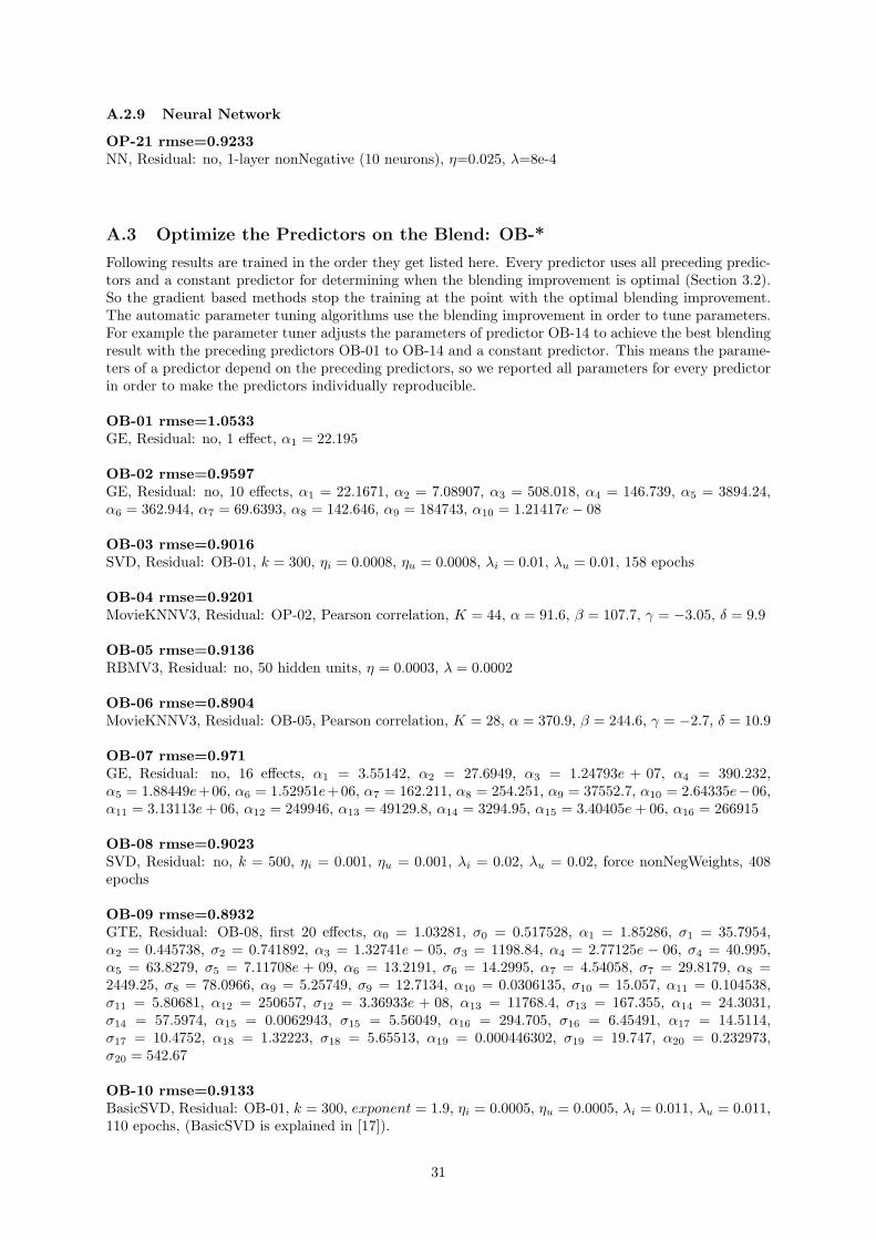
A.2.9 Neural Network

OP-21 rmse=0.9233NN, Residual: no, 1-layer nonNegative (10 neurons), η=0.025, λ=8e-4

A.3 Optimize the Predictors on the Blend: OB-*

Following results are trained in the order they get listed here. Every predictor uses all preceding predic-tors and a constant predictor for determining when the blending improvement is optimal (Section 3.2).So the gradient based methods stop the training at the point with the optimal blending improvement.The automatic parameter tuning algorithms use the blending improvement in order to tune parameters.For example the parameter tuner adjusts the parameters of predictor OB-14 to achieve the best blendingresult with the preceding predictors OB-01 to OB-14 and a constant predictor. This means the parame-ters of a predictor depend on the preceding predictors, so we reported all parameters for every predictorin order to make the predictors individually reproducible.

OB-01 rmse=1.0533GE, Residual: no, 1 effect, α1 = 22.195

OB-02 rmse=0.9597GE, Residual: no, 10 effects, α1 = 22.1671, α2 = 7.08907, α3 = 508.018, α4 = 146.739, α5 = 3894.24,α6 = 362.944, α7 = 69.6393, α8 = 142.646, α9 = 184743, α10 = 1.21417e− 08

OB-03 rmse=0.9016SVD, Residual: OB-01, k = 300, ηi = 0.0008, ηu = 0.0008, λi = 0.01, λu = 0.01, 158 epochs

OB-04 rmse=0.9201MovieKNNV3, Residual: OP-02, Pearson correlation, K = 44, α = 91.6, β = 107.7, γ = −3.05, δ = 9.9

OB-05 rmse=0.9136RBMV3, Residual: no, 50 hidden units, η = 0.0003, λ = 0.0002

OB-06 rmse=0.8904MovieKNNV3, Residual: OB-05, Pearson correlation, K = 28, α = 370.9, β = 244.6, γ = −2.7, δ = 10.9

OB-07 rmse=0.971GE, Residual: no, 16 effects, α1 = 3.55142, α2 = 27.6949, α3 = 1.24793e + 07, α4 = 390.232,α5 = 1.88449e+06, α6 = 1.52951e+06, α7 = 162.211, α8 = 254.251, α9 = 37552.7, α10 = 2.64335e−06,α11 = 3.13113e+ 06, α12 = 249946, α13 = 49129.8, α14 = 3294.95, α15 = 3.40405e+ 06, α16 = 266915

OB-08 rmse=0.9023SVD, Residual: no, k = 500, ηi = 0.001, ηu = 0.001, λi = 0.02, λu = 0.02, force nonNegWeights, 408epochs

OB-09 rmse=0.8932GTE, Residual: OB-08, first 20 effects, α0 = 1.03281, σ0 = 0.517528, α1 = 1.85286, σ1 = 35.7954,α2 = 0.445738, σ2 = 0.741892, α3 = 1.32741e − 05, σ3 = 1198.84, α4 = 2.77125e − 06, σ4 = 40.995,α5 = 63.8279, σ5 = 7.11708e + 09, α6 = 13.2191, σ6 = 14.2995, α7 = 4.54058, σ7 = 29.8179, α8 =2449.25, σ8 = 78.0966, α9 = 5.25749, σ9 = 12.7134, α10 = 0.0306135, σ10 = 15.057, α11 = 0.104538,σ11 = 5.80681, α12 = 250657, σ12 = 3.36933e + 08, α13 = 11768.4, σ13 = 167.355, α14 = 24.3031,σ14 = 57.5974, α15 = 0.0062943, σ15 = 5.56049, α16 = 294.705, σ16 = 6.45491, α17 = 14.5114,σ17 = 10.4752, α18 = 1.32223, σ18 = 5.65513, α19 = 0.000446302, σ19 = 19.747, α20 = 0.232973,σ20 = 542.67

OB-10 rmse=0.9133BasicSVD, Residual: OB-01, k = 300, exponent = 1.9, ηi = 0.0005, ηu = 0.0005, λi = 0.011, λu = 0.011,110 epochs, (BasicSVD is explained in [17]).

31

OB-11 rmse=0.9608SVD-ALS, Residual: no, k = 5, movieSolver=nonNeg, userSolver=nonNeg, λi = 0.15, λu = 0.15, 479epochs

OB-12 rmse=0.9933WE, Residual: OB-01, regU=7.61098 regM=4.27357e+10 regGlob=1.25265e+10 powGlob=0.00033654powM=0.0310857 powU=3.445

OB-13 rmse=0.9093SVD, Residual: no, k = 1000, ηi = 0.01, ηu = 0.008, λi = 0.01, λu = 0.04, force nonNegativeWeights,with user and movie biases, 60 epochs

OB-14 rmse=0.9197MovieKNNV3, Residual: OB-11, Spearman’s rank correlation, K = 14, α = 280, β = 3572, γ = −3,δ = 8.34

OB-15 rmse=0.8878CTD, Residual: OB-06, weightingFctn=GAUSSIAN-WEIGHT, α = 77.3653, β = 11.43 γ = 0.971957

OB-16 rmse=1.0047SVD-ALS, Residual: OB-01, k = 300, λi = 0.01, λu = 0, movieSolver=PINV, userSolver=PINV, 9epochs

OB-17 rmse=0.9135MovieKNNV3, Residual: OB-16, MSE correlation, K = 34, α = 204.8, β = 1889, γ = −3.8, δ = 7

OB-18 rmse=0.9036RBMV5, Residual: OB-07, 300 hidden units, η = 0.0002, λ = 0.0007


OB-20 rmse=0.8925MovieKNNV3, Residual: OB-09, MSE correlation, K = 150, α = 2170.7, β = 165.4, γ = −2.6, δ = 1

OB-21 rmse=0.8923MovieKNNV3, Residual: OB-09, Pearson correlation, K = 203, α = 657.8, β = 3043, γ = −4.17,δ = 31.8

OB-22 rmse=0.9774MovieKNNV3, Residual: no, Pearson correlation, K = 94, α = 137.2, β = 1963, γ = −3, δ = 8

OB-23 rmse=0.9317NSVD1, Residual: no, k = 40, ηi = 1e − 4, ηu = 1e − 4, ηµi

= 2e − 3, ηµu= 2e − 3, λi = 1e − 3,

λu = 1e− 3, λµi = 2e− 3, λµu = 2e− 3, muliply all η with 0.9 from epoch 40, 96 epochs

OB-24 rmse=0.899SVD-AUF, Residual: OB-23, adaptiveUserFactorMode=KRR, kernelType=polynomial, λ = 29.1733,α = 0.39171, β = 3.64831

OB-25 rmse=0.9517SVD-AUF, Residual: OB-11, adaptiveUserFactorMode=dateSim, solver=PINV, λ = 0.00243, γ1.31035,β = 0.356343, κ = −0.0165


32

OB-27 rmse=1.0202GTE, Residual: no, 24 effects, α0 = 0.756448, σ0 = 63.3648, α1 = 0.000341077, σ1 = 783.599,α2 = 7.66667, σ2 = 2.22136, α3 = 441.092, σ3 = 2.39512, α4 = 7.9987, σ4 = 2.30299, α5 = 2.19463,σ5 = 2.50274, α6 = 0.40246, σ6 = 3.79979, α7 = 0.00869847, σ7 = 0.190355, α8 = 3761.7, σ8 = 49.564,α9 = 0.0289626, σ9 = 2.16438, α10 = 0.174869, σ10 = 7.87177, α11 = 0.723074, σ11 = 0.258699,α12 = 358857, σ12 = 8.36612, α13 = 0.415689, σ13 = 0.342104, α14 = 0.719413, σ14 = 5.46462, α15 =0.278113, σ15 = 2.01964, α16 = 2.9132, σ16 = 0.540534, α17 = 0.291892, σ17 = 5.01496, α18 = 1.06935,σ18 = 14.0819, α19 = 0.000909, σ19 = 8.7371, α20 = 3.33668, σ20 = 3.6388, α21 = 124644, σ21 = 2.39229,α22 = 2.19671, σ22 = 4.83657, α23 = 3.74613, σ23 = 1.37054, α24 = 1.59059, σ24 = 1.59185

OB-28 rmse=0.9226SVD-AUF, Residual: OB-08, adaptiveUserFactorMode=KRR, kernelType=extended-polynomial, λ =7.08585, α = 0.109493, γ = 0.495312, β = 0.00834611

OB-29 rmse=0.915SVD-AUF, Residual: OB-13, adaptiveUserFactorMode=KRR, kernelType=polynomial, λ = 12.6179,α = 0.790135, β = 5.13577

OB-30 rmse=0.9283NSVD1, Residual: OB-27, k = 1000, ηi = 1e− 4, ηu = 1e− 4, ηµi

= 2e− 3, ηµu= 2e− 3, λi = 1.5e− 3,

λu = 1.5e− 3, λµi= 2e− 3, λµu

= 2e− 3, muliply all η with 0.95 from epoch 35, 150 epochs

OB-31 rmse=0.9022MovieKNNV3, Residual: OB-30, Pearson correlation, K = 35, α = 291.3, β = 571, γ = −2.9, δ = 18.9



OB-34 rmse=0.927SVD-Time, Residual: globalMean, k = 50, N = 5, M = 5, ηi = 0.002, ηu = 0.002, λi = 0.01, λu = 0.03,96 epochs


OB-36 rmse=0.9104SVD-Time, Residual: OB-26, k = 20, N = 4, M = 4, ηi = 0.002, ηu = 0.002, λi = 0.02, λu = 0.02, 158epochs


OB-38 rmse=0.8978MovieKNNV3, Residual: OB-37, Spearman’s rank correlation, K = 225, α = 112.6, β = 1922, γ = −3.2,δ = 9.3

OB-39 rmse=0.9213NSVD1, Residual: OB-02, k = 800, ηi = 1e − 4, ηu = 1e − 4, ηµi = 2e − 3, ηµu = 2e − 3, λi = 5e − 4,λu = 5e− 4, λµi = 2e− 3, λµu = 2e− 3, muliply all η with 0.97 from epoch 35, 200 epochs


OB-41 rmse=0.913RBMV5, Residual: globalMean, 1000 hidden units, η = 0.0002, λ = 0.0009

33

OB-42 rmse=0.8998MovieKNNV3, Residual: OB-39, Pearson correlation, K = 13, α = 658, β = 2480, γ = −2.6, δ = 7.5

OB-43 rmse=0.8971SVD-AUF, Residual: OB-30, adaptiveUserFactorMode=KRR, kernelType=extended-polynomial, λ =4.78376, α = 0.657533, γ = 0.720031, β = 3.27554

OB-44 rmse=0.9245GE, Residual: OB-35, 16 effects, α1 = 374.977, α2 = 8.90702e − 05, α3 = 2535.9, α4 = 900.414,α5 = 1.04115e−05, α6 = 2087.92, α7 = 131.291, α8 = 3173.84, α9 = 1.45471e−06, α10 = 6.40823e−08,α11 = 4451.15, α12 = 274.423, α13 = 1020.64, α14 = 0.00758424, α15 = 3858.57, α16 = 0.00346888

OB-45 rmse=0.8998MovieKNNV3, Residual: OB-40, Spearman’s rank correlation, K = 38, α = 667.6, β = 255.5, γ = −1.39,δ = 3.3

OB-46 rmse=0.8958MovieKNNV3, Residual: OB-41, Pearson correlation, K = 60, α = 804, β = 231, γ = −2.6, δ = 17

OB-47 rmse=0.9777NSVD2, Residual: no, k = 50, ηi = 2e − 3, ηu = 2e − 3, ηµi = 2e − 3, ηµu = 2e − 3, λi = 5e − 4,λu = 5e− 4, λµi = 1e− 4, λµu = 1e− 4, 3 epochs

OB-48 rmse=0.9344NSVDD, Residual: no, k = 200, ηi = 1e − 3, ηu = 1e − 3, ηµi

= 1e − 3, ηµu= 1e − 3, λi = 1e − 3,

λu = 1e− 3, λµi= 1e− 3, λµu


OB-49 rmse=0.9205MovieKNNV3, Residual: OB-47, Pearson correlation, K = 17, α = 274.6, β = 1712, γ = −2.9, δ = 20


OB-51 rmse=0.9016GE, Residual: OB-50, 16 effects, α1 = 172.971, α2 = 633.616, α3 = 278.061, α4 = 479.608, α5 = 571.286,α6 = 17550.3, α7 = 41.7332, α8 = 107.62, α9 = 8089.62, α10 = 1510.79, α11 = 3.28767e − 05,α12 = 38.4236, α13 = 78.8427, α14 = 0.00298945, α15 = 695035, α16 = 0.0409925


OB-53 rmse=0.9178SVD-Time, Residual: OB-49, k = 70, N = 6, M = 3, ηi = 0.003, ηu = 0.003, λi = 0.025, λu = 0.045,106 epochs

OB-54 rmse=0.9641SVD-Time, Residual: OB-01, k = 20, N = 6, M = 8, ηi = 0.002, ηu = 0.002, λi = 0.01, λu = 0.02, 22epochs


OB-56 rmse=0.9298MovieKNNV3, Residual: OB-54, Pearson correlation, K = 168, α = 1012, β = 523, γ = −3.2, δ = 7

OB-57 rmse=0.9017GTE, Residual: OB-52, 24 effects, α0 = 1.00571, σ0 = 3.61101, α1 = 5.14906, σ1 = 15.2058, α2 =

34

0.253872, σ2 = 3.85881, α3 = 6.44612, σ3 = 18.5493, α4 = 0.49935, σ4 = 3.63728, α5 = 0.430758,σ5 = 6.03448, α6 = 30.0492, σ6 = 9.40765, α7 = 1.06677, σ7 = 26.7225, α8 = 1.04277e − 05,σ8 = 2.49227, α9 = 49.0741, σ9 = 0.262239, α10 = 5.13061, σ10 = 17.0218, α11 = 1.7518, σ11 = 3.44103,α12 = 0.193035, σ12 = 5.10717, α13 = 2950.42, σ13 = 2.07498, α14 = 17.3151, σ14 = 14.2747,α15 = 0.0108529, σ15 = 5.62521, α16 = 8.30796, σ16 = 5.64531, α17 = 5.79247, σ17 = 2.20745,α18 = 0.318347, σ18 = 1.17436, α19 = 2.11259e − 10, σ19 = 11.1742, α20 = 606.263, σ20 = 1.38733,α21 = 1666.74, σ21 = 1.21059, α22 = 11.9562, σ22 = 3.85147, α23 = 12.9199, σ23 = 10.8872, α24 =81.5603, σ24 = 14.5512


OB-59 rmse=0.8932MovieKNNV3, Residual: OB-58, Spearman’s rank correlation, K = 74, α = 725.6, β = 94.8, γ = −3.6,δ = 12.4

OB-60 rmse=1.0207MMMF, Residual: no, k = 200, ηi = 0.001, ηu = 0.001, λi = 0.01, λu = 0.01, 185 epochs


= 2e − 3, ηµu= 2e − 3, λi = 1e − 3,



OB-63 rmse=0.9651GE, Residual: no, 16 effects, α1 = 4.76342e − 06, α2 = 2.2696, α3 = 135.319, α4 = 103.14, α5 =0.000150371, α6 = 585.235, α7 = 158997, α8 = 61.2179, α9 = 332.361, α10 = 1.38317e − 07, α11 =119256, α12 = 124.482, α13 = 1553.02, α14 = 9.50186e− 07, α15 = 125357, α16 = 3.36691e+ 11


OB-65 rmse=0.9331GE, Residual: OB-64, 16 effects, α1 = 1.34006e−07, α2 = 5.3791e−09, α3 = 4.43366e−05, α4 = 271975,α5 = 2588.31, α6 = 43.7395, α7 = 27.2455, α8 = 20.2169, α9 = 0.000139488, α10 = 6.77118e − 06,α11 = 2.06308e − 05, α12 = 896427, α13 = 0.000959451, α14 = 80901.1, α15 = 9.15078e + 07,α16 = 0.00011957

OB-66 rmse=0.9338NSVDD, Residual: OB-63, k = 1000, ηi = 1e− 3, ηu = 1e− 3, ηµi

= 1e− 3, ηµu= 1e− 3, λi = 5e− 3,

λu = 5e− 3, λµi= 5e− 3, λµu

= 5e− 3, 2 epochs

OB-67 rmse=0.9127NSVDD, Residual: OB-65, k = 2000, ηi = 1e− 3, ηu = 1e− 3, ηµi = 1e− 3, ηµu = 1e− 3, λi = 2e− 3,λu = 2e− 3, λµi

= 1.5e− 3, λµu= 1.5e− 3, 23 epochs


OB-69 rmse=0.91GTE, Residual: OB-67, 24 effects, α0 = 0.460297, σ0 = 0.112732, α1 = 5.07411, σ1 = 24.9513,α2 = 0.000821287, σ2 = 1.31449, α3 = 26.0328, σ3 = 53.549, α4 = 0.0370089, σ4 = 3.11902,α5 = 53.8362, σ5 = 0.131344, α6 = 5.97711, σ6 = 4.25552, α7 = 6.22559, σ7 = 19.656, α8 = 588.765,σ8 = 26.7259, α9 = 7.44892, σ9 = 9.49731, α10 = 0.00456163, σ10 = 97.7392, α11 = 0.0455336, σ11 =38.9575, α12 = 0.278585, σ12 = 2.80386, α13 = 31.7377, σ13 = 16.273, α14 = 864.606, σ14 = 37.458,α15 = 0.00166922, σ15 = 4.53062, α16 = 1444.98, σ16 = 1.42299, α17 = 295.419, σ17 = 9.83184,

35

α18 = 1.59155, σ18 = 1.42808e + 09, α19 = 0.216866, σ19 = 16.3573, α20 = 78.8341, σ20 = 7.42034,α21 = 26.3644, σ21 = 11.8044, α22 = 7.49029, σ22 = 28.4897, α23 = 1, σ23 = 1, α24 = 53.8362,σ24 = 1.7108

OB-70 rmse=0.9136SVD-ALS, Residual: no, k = 50, movieSolver=nonNeg, userSolver=nonNeg, λi = 0.05, λu = 0.05, 47epochs

OB-71 rmse=0.9122SVD-AUF, Residual: OB-70, adaptiveUserFactorMode=Pearson, solver=PINV, λ = 0.0289428, α =20.1176, δ = 8.55221 γ = −8.5, κ = 0.00640817

OB-72 rmse=0.9099GE, Residual: OB-71, 16 effects, α1 = 0.0014015, α2 = 3.99785, α3 = 207.554, α4 = 213.329,α5 = 59340.4, α6 = 1512.75, α7 = 46.0147, α8 = 103.674, α9 = 0.00256827, α10 = 1.92437e − 05,α11 = 21.961, α12 = 5.55441, α13 = 82.6428, α14 = 3044.49, α15 = 53.7824, α16 = 2244.73

OB-73 rmse=0.9063NSVD1, Residual: OB-72, k = 280, ηi = 1e − 3, ηu = 1e − 3, ηµi

= 2e − 4, ηµu= 2e − 4, λi = 1e − 6,

λu = 1e− 6, λµi= 1e− 5, λµu


OB-74 rmse=0.9724SVD-Time, Residual: OB-63, k = 500, N = 30, M = 30, ηi = 0.001, ηu = 0.001, λi = 0.01, λu = 0.01,333 epochs

OB-75 rmse=1.0203GTE, Residual: no, 24 effects, α0 = 0.756448, σ0 = 63.3648, α1 = 0.000341077, σ1 = 783.599,α2 = 7.66667, σ2 = 2.22136, α3 = 441.092, σ3 = 2.39512, α4 = 7.9987, σ4 = 2.30299, α5 = 2.19463,σ5 = 2.50274, α6 = 0.40246, σ6 = 3.79979, α7 = 0.00869847, σ7 = 0.190355, α8 = 3761.7, σ8 = 49.564,α9 = 0.0289626, σ9 = 2.16438, α10 = 0.174869, σ10 = 7.87177, α11 = 0.723074, σ11 = 0.258699,α12 = 358857, σ12 = 8.36612, α13 = 0.415689, σ13 = 0.342104, α14 = 0.719413, σ14 = 5.46462,α15 = 0.278113, σ15 = 2.01964, α16 = 2.9132, σ16 = 0.540534, α17 = 0.291892, σ17 = 5.01496,α18 = 1.06935, σ18 = 14.0819, α19 = 0.000909059, σ19 = 8.7371, α20 = 3.33668, σ20 = 3.6388, α21 =124644, σ21 = 2.39229, α22 = 2.19671, σ22 = 4.83657, α23 = 3.74613, σ23 = 1.37054, α24 = 1.59059,σ24 = 1.59185



OB-78 rmse=0.9686NSVD2, Residual: OB-75, k = 2000, ηi = 1e− 3, ηu = 1e− 3, ηµi

= 1e− 3, ηµu= 1e− 3, λi = 1e− 6,


OB-79 rmse=0.9471NSVDD, Residual: no, k = 2000, ηi = 1e − 3, ηu = 1e − 3, ηµi

= 1e − 3, ηµu= 1e − 3, λi = 4e − 2,

λu = 4e− 2, λµi= 5e− 2, λµu


OB-80 rmse=0.9029MovieKNNV3-2, Residual: OB-79, Pearson correlation, K = 78, α = 1021, β = 858, γ = −3.5, δ = 12.2,ζ = 0.9, ϑ = 0.9, κ = 0.9, ν = 0, ψ = 1

OB-81 rmse=0.9612GE, Residual: OB-71, 16 effects, α1 = 4.16513, α2 = 1.7129e − 06, α3 = 456.842, α4 = 178.695,α5 = 553.964, α6 = 7680.3, α7 = 223.568, α8 = 181.913, α9 = 2.43476e − 06, α10 = 4.40681e − 06,α11 = 8098.95, α12 = 261.822, α13 = 243.656, α14 = 550.911, α15 = 2175.92, α16 = 6686.61

36

OB-82 rmse=0.9334MovieKNNV3-2, Residual: OB-81, Pearson correlation, K = 71, α = 0.28, β = 716, γ = −1.9, δ = 18.2,ζ = 1, ϑ = 0.22, κ = 1.1, ν = −0.002, ψ = 1


= 1e − 3, ηµu= 1e − 3, λi = 1e − 3,

λu = 1e− 2, λµi= 1e− 3, λµu


OB-84 rmse=1.1148MovieKNNV3-2, Residual: no, Ratio correlation, K = 14, α = 2.5, β = 9825, γ = −9.5, δ = 4.4, ζ = 1,ϑ = 2.2, κ = 1, ν = 0, ψ = 1

OB-85 rmse=1.01MovieKNNV3-2, Residual: OB-83, Ratio correlation, K = 26, α = 0.5, β = 1207, γ = −7.4, δ = 4.86,ζ = 1, ϑ = 1.7, κ = 1.05, ν = −0.02, ψ = 1

OB-86 rmse=0.9534NSVDD, Residual: OB-02, k = 20, ηi = 1e − 3, ηu = 1e − 2, ηµi

= 1e − 3, ηµu= 1e − 3, λi = 1e − 2,

λu = 1e− 3, λµi= 5e− 3, λµu

= 5e− 3, 7 epochs

OB-87 rmse=0.9468MovieKNNV3-2, Residual: OB-86, MSE correlation, K = 24, α = 47.4, β = 129, γ = −6, δ = 5, ζ = 1,ϑ = 2.6, κ = 1.1, ν = 0, ψ = 1

OB-88 rmse=0.928SVD-AUF, Residual: OB-83, adaptiveUserFactorMode=KRR, kernelType=pow, λ = 9.35378, α = 0.1,γ = 0.2, κ = 1.04

OB-89 rmse=0.9228GTE, Residual: OB-88, 24 effects, α0 = 2.3976, σ0 = 4.14296, α1 = 5.48903e − 06, σ1 = 13.3131,α2 = 1.4251, σ2 = 1.2055, α3 = 0.0394946, σ3 = 1.53379e + 07, α4 = 5.22812, σ4 = 9.03679,α5 = 0.837984, σ5 = 2.38426, α6 = 1.30288, σ6 = 6.80418, α7 = 3.46388e − 10, σ7 = 0.98697,α8 = 902.531, σ8 = 0.565299, α9 = 6.0307, σ9 = 2.16438, α10 = 2.80001, σ10 = 0.612924, α11 = 251.787,σ11 = 2.16069, α12 = 63023.2, σ12 = 1.89939, α13 = 1.42503e − 08, σ13 = 18.3012, α14 = 3.23376,σ14 = 2.64433, α15 = 3237.21, σ15 = 5.45511, α16 = 50.9026, σ16 = 1.27025e + 08, α17 = 829.237,σ17 = 15.3857, α18 = 5.27389, σ18 = 53.1659, α19 = 0.385785, σ19 = 1.59994, α20 = 0.00453852,σ20 = 4.15031, α21 = 0.00351637, σ21 = 0.444039, α22 = 0.864983, σ22 = 0.282021, α23 = 0.236967,σ23 = 4.84254, α24 = 3.29083, σ24 = 4.51019

OB-90 rmse=0.8885SVD++, Residual: no, k = 1200, ηi = 5e − 3, ηu = 5e − 3, ηy = 1e − 3 ηµi

= 1e − 3, ηµu= 1e − 3,

λi = 1.5e− 2, λu = 1.5e− 2, λy = 1.0e− 2, λµi= 1.5e− 2, λµu

= 1.5e− 2, 77 epochs

OB-91 rmse=0.8806IM, Residual: no, k = 150, nMovieTimeBins=10, muliply all η with 0.95 from epoch 13, 59 epochs


OB-93 rmse=0.8968MovieKNNV3-2, Residual: OB-92, Pearson correlation, K = 24, α = 2837, β = 159, γ = −4.7, δ = 7,ζ = 1, ϑ = 0.8, κ = 1, ν = 0, ψ = 1

OB-94 rmse=0.8818IM, Residual: no, k = 50, nMovieTimeBins=20, muliply all η with 0.95 from epoch 13, 49 epochs

OB-95 rmse=0.9202

37

IM, Residual: no, k = 10, nMovieTimeBins=20, 98 epochs

OB-96 rmse=0.8896SBRAMF-UTB-UTF, Residual: no, k = 150, 198 epochs

OB-97 rmse=0.9148SVD++Sym, Residual: no, k = 10, 16 epochs

OB-98 rmse=0.8788SBRAMF-UTB-UTF-MTF-ATF-MFF-AFF, Residual: no, k = 150, 62 epochs

OB-99 rmse=0.9466MovieKNNV3-2, Residual: OB-78, Pearson correlation, K = 31, α = 546, β = 2030, γ = −2.67, δ = 7,ζ = 0.8, ϑ = 3.17, κ = 0.48, ν = 0, ψ = 1

OB-100 rmse=0.8758MovieKNNV3-2, Residual: OB-98, Pearson correlation, K = 141, α = 1204, β = 332, γ = −4.1,δ = 21.7, ζ = 1, ϑ = 0.4, κ = 1, ν = 0, ψ = 1

OB-101 rmse=0.8752GE, Residual: OB-100, 16 effects, α1 = 0.000129761, α2 = 1.22704e − 05, α3 = 13.8956, α4 = 956.858,α5 = 0.000183497, α6 = 93953.6, α7 = 2.36624e − 05, α8 = 95.9403, α9 = 282.937, α10 = 184.181,α11 = 0.0208714, α12 = 62.7879, α13 = 253.117, α14 = 11940.3, α15 = 52600.9, α16 = 93.6713

A.4 Optimize the Predictors on the Blend and Correct Residuals

For the following predictors we used a K = 34 cross fold (3.3). So we have 34 probe/qualifying predic-tions for a individual predictor. The reported RMSE values are based on a linear probe blend of this 34predictors.

OBC-01 rmse=0.8977SVD, Residual: no, k = 200, ηi = 0.002, ηu = 0.002, λi = 0.01, λu = 0.01, with biases, 61 epochs

OBC-02 rmse=0.8974KNNMovieV2-2, Residual: OBC-01, Pearson correlation, K = 50, α = 842.5, β = 144.2, γ = −5.3,δ = 25.9, ζ = 0.98, ϑ = 1.47, κ = 0.5, ν = 0.5, ψ = 0.015

OBC-03 rmse=0.8935KNNMovieV2-2, Residual: OBC-01, Spearman’s rank correlation, K = 30, α = 82.5, β = 9.8, γ = 0.037,δ = 0.76, ζ = 1.0, ϑ = 1.13, κ = 1.2, ν = −0.1, ψ = 0.46

OBC-04 rmse=0.9007RBMV3, Residual: no, 100 hidden units, η = 0.0012, λ = 0.00025

OBC-05 rmse=0.8845KNNMovieV2-2, Residual: OBC-04, Pearson correlation, K = 39, α = 5889, β = 410.5, γ = 0.0034,δ = 6.7, ζ = 1.96, ϑ = 2.3, κ = 1.2, ν = −0.001, ψ = 0.69

OBC-06 rmse=0.8797GTE, Residual: OBC-05, 24 effects, α0 = 0.00526644, σ0 = 0.752045, α1 = 0.0262868, σ1 = 67.7921,α2 = 1.00398e − 09, σ2 = 0.145604, α3 = 0.489294, σ3 = 958.148, α4 = 0.0791142, σ4 = 0.906078,α5 = 0.000544352, σ5 = 985.25, α6 = 1.59343, σ6 = 4.98191, α7 = 1.52602, σ7 = 20.1282, α8 = 856.134,σ8 = 80.9295, α9 = 1.17037, σ9 = 92.1946, α10 = 35473.3, σ10 = 19.8605, α11 = 1.0084, σ11 = 7.89876,α12 = 2.1725e + 07, σ12 = 167.712, α13 = 3237.21, σ13 = 6.10341e + 12, α14 = 7583.2, σ14 = 91.7444,α15 = 593.311, σ15 = 0.564514, α16 = 0.170086, σ16 = 113.133, α17 = 1.0753, σ17 = 64.5719, α18 =28673.5, σ18 = 288.548, α19 = 0.326539, σ19 = 15.2178, α20 = 0.00497239, σ20 = 17.0848, α21 = 1.98397,σ21 = 9.45723, α22 = 20.8867, σ22 = 9.66172, α23 = 9.03199, σ23 = 4.75582, α24 = 0.00154022,σ24 = 3.76928

38

OBC-07 rmse=0.8899SVD++, Residual: no, k = 250, ηi = 5e − 3, ηu = 5e − 3, ηy = 1e − 3 ηµi

= 1e − 3, ηµu= 1e − 3,

λi = 1.5e− 2, λu = 1.5e− 2, λy = 1.0e− 2, λµi= 1.5e− 2, λµu

= 1.5e− 2, 39 epochs

OBC-08 rmse=0.9046SVD-ALS, Residual: no, k = 100, movieSolver=nonNeg, userSolver=nonNeg, λi = 0.05, λu = 0.05, 13epochs

OBC-09 rmse=0.9009SVD-AUF, Residual: OBC-08, adaptiveUserFactorMode=dateSim, solver=nonNeg, λ = 0.0403887,γ = 0.195976, β = 0.191341, κ = 0.0168

OBC-10 rmse=0.8826IM, Residual: no, k = 50, nMovieTimeBins=20, 39 epochs

A.5 Probe Blending Results

A.5.1 BigChaos - Probe Predictors Blends

—[Mixes of subsets]—

PB-001 rmse=0.9230NNBlend, Predictors OP-12,OP-16,OP-18, 1HL, 10 neurons, η(−) = 3e− 7, 1334 epochs

PB-002 rmse=0.9102NNBlend, Predictors OP-14,OP-16,OP-18,OP-19,OP-20, 1HL, 10 neurons, η(−) = 3e− 7, 1334 epochs

PB-003 rmse=0.8805NNBlend, Predictors OP-01..OP-06 , 1HL, 20 neurons, η(−) = 3e− 7, 1334 epochs



PB-006 rmse=0.8694NNBlend, Predictors BC-ProbeOpt-21, PP-01..PP-12,, 1HL, 20 neurons, η(−) = 3e− 7, 1334 epochs

PB-007 rmse=0.8685NNBlend, Predictors BC-ProbeOpt-21, PP-01..PP-29, 1HL, 20 neurons, η(−) = 3e− 7, 1334 epochs






PB-013 rmse=0.8674

39

Group Name count Description

BC-Exact-10 10 Predictions from BigChaos, generated by the correct residual framwork OBC-01..OBC-10BC-Exact-340 340 Predictions from BigChaos, OBC-01..OBC-10, all results from the 34-cross-fold setupBC-BlendOpt-101 101 Predictions from BigChaos, generated by the optimize on blend framwork OB-01..OB-101BC-PPrize08-60 60 Subset of predictions from BigChaos 2008 Progress Prize results PP-01..PP-60BC-PPrize08-95 95 Predictions from BigChaos 2008 Progress Prize results 1..95BC-ProbeOpt-21 21 Single results, optimizing the probe RMSE, OP-01..OP-21BC-132 132 BigChaos results BC-Exact-10,BC-BlendOpt-101,BC-ProbeOpt-21BC-171 171 BigChaos results BC-Exact-10,BC-BlendOpt-101,BC-PPrize08-60BC-192 192 BigChaos results BC-Exact-10,BC-BlendOpt-101,BC-PPrize08-60,BC-ProbeOpt-21BC-192-Top5 5 Forward selection on BC-192, best 5 resultsBC-192-Top10 10 Forward selection on BC-192, best 10 resultsBC-192-Top15 15 Forward selection on BC-192, best 15 resultsBC-192-Top20 20 Forward selection on BC-192, best 20 resultsBC-192-Top15 25 Forward selection on BC-192, best 25 resultsBC-192-Top30 30 Forward selection on BC-192, best 30 resultsBC-192-Top35 35 Forward selection on BC-192, best 35 resultsPT-236 236 Predictions from Pragmatic Theory received on April, 21th 2009PT-236-Top10 10 Forward selection on PT-236, best 10 resultsPT-236-Top20 20 Forward selection on PT-236, best 20 resultsPT-236-Top30 30 Forward selection on PT-236, best 30 resultsPT-236-Top40 40 Forward selection on PT-236, best 40 resultsPT-236-Top50 50 Forward selection on PT-236, best 50 resultsPT-236-Top60 60 Forward selection on PT-236, best 60 resultsPT-236-Top70 70 Forward selection on PT-236, best 70 resultsPT-236-Top80 80 Forward selection on PT-236, best 80 resultsPT-236-Top90 90 Forward selection on PT-236, best 90 resultsPT-236-Top100 100 Forward selection on PT-236, best 100 resultsPT-236-Top110 110 Forward selection on PT-236, best 110 resultsPT-236-Top120 120 Forward selection on PT-236, best 120 resultsPT-236-Top130 130 Forward selection on PT-236, best 130 resultsPT-236-Top140 140 Forward selection on PT-236, best 140 resultsPT-242 242 PT-236 and 6 PT resultsPT-242-PQDiff00-49 43 PT-242 results with d = RMSEprobe − RMSEquiz, d ≤ 0.0049PT-242-PQDiff50-62 49 PT-242 results with 0.0063 ≥ d > 0.0049PT-242-PQDiff63-73 48 PT-242 results with 0.0073 ≥ d > 0.0063PT-242-PQDiff74-82 50 PT-242 results with 0.0082 ≥ d > 0.0073PT-242-PQDiff83-99 52 PT-242 results with 0.0083 < dPT-250 250 PT-242 and 8 PT resultsPT-250-Bottom10 10 Forward selection on PT-250, take last 10 (the results which are least significant)PT-250-Bottom20 20 Forward selection on PT-250, take last 20PT-250-Bottom30 30 Forward selection on PT-250, take last 30PT-250-Bottom40 40 Forward selection on PT-250, take last 40PT-250-Bottom50 50 Forward selection on PT-250, take last 50PT-250-Bottom60 60 Forward selection on PT-250, take last 60PT-250-Bottom70 70 Forward selection on PT-250, take last 70PT-250-Bottom80 80 Forward selection on PT-250, take last 80PT-250-Bottom90 90 Forward selection on PT-250, take last 90PT-282 282 PT-236 and 46 PT resultsPT-168 168 A set from PT were only probe RMSEs are availablePT-New16 16 16 results from PT received on May, 30th 2009SVD++10-94 94 Predictors extracted from a 10-dim SBRAMF-UTB-UTF-MTF-ATF-MFF-AFF modelSVD++10-cross-144 144 Predictors extracted from a 10-dim SBRAMF-UTB-UTF-MTF-ATF-MFF-AFF model, with cross interactionsSVD++20-186 186 Predictors extracted from a 20-dim SBRAMF-UTB-UTF-MTF-ATF-MFF-AFF modelSVD++50-454 454 Predictors extracted from a 50-dim SBRAMF-UTB-UTF-MTF-ATF-MFF-AFF modelRBM-20-user 20 Activation values from the hidden unit layer (user as a bag of movies), 20 unit discrete RBMRBM-20-movie 20 Activation values from the hidden unit layer (movie as a bag of users), 20 unit discrete RBMRBM-20-movieWeights 120 Visible to hidden weights 5x discrete, 1x conditional, 20 unit Discrete RBMRBM-50-user 50 Activation values from the hidden unit layer, 50 unit Discrete RBMKNNk3-101 1515 KNN feature extraction, k = 3 neighbors, on all optimize on blend results (OB-01..OB-101)KNNk50-OB-52-250 250 KNN feature extraction, k = 50, on OB-52 (RBMV5)BK-results-17 17 BellKor results from Progress Prize 2008BK-results-6 6 BellKor results, 2009ALL-391 391 Merged results from all 3 teams: PT-236,BC-132,BK-results-17,BK-results-6ALL-391-Top3 3 Forward selection on ALL-391, best 3 resultsALL-391-Top4 4 Forward selection on ALL-391, best 4 resultsALL-391-Top5 5 Forward selection on ALL-391, best 5 resultsALL-391-Top10 10 Forward selection on ALL-391, best 10 resultsALL-391-Top20 20 Forward selection on ALL-391, best 20 resultsALL-391-Top30 30 Forward selection on ALL-391, best 30 resultsALL-391-Top40 40 Forward selection on ALL-391, best 40 resultsALL-391-Top50 50 Forward selection on ALL-391, best 50 resultsALL-391-Top60 60 Forward selection on ALL-391, best 60 resultsALL-391-Top70 70 Forward selection on ALL-391, best 70 resultsALL-391-Top80 80 Forward selection on ALL-391, best 80 resultsALL-391-Top90 90 Forward selection on ALL-391, best 90 resultsALL-391-Top100 100 Forward selection on ALL-391, best 100 resultsALL-391-Top110 110 Forward selection on ALL-391, best 110 resultsALL-391-Top120 120 Forward selection on ALL-391, best 120 resultsALL-391-Top130 130 Forward selection on ALL-391, best 130 resultsALL-391-Top140 140 Forward selection on ALL-391, best 140 resultsALL-391-Bottom40 40 Forward selection on ALL-391, take last 40ALL-476 476 Merged results from all 3 teams: BC-171, PT-282, BK-results-17, BK-results-6ALL-476-Top75 75 Forward selection on ALL-476, best 75 results

Table 10: Different sets of results used for probe blending.

40

NNBlend, Predictors BC-ProbeOpt-21, PP-01..PP-48, 1HL, 15 neurons, η(−) = 3e− 7, 1334 epochs





PB-018 rmse=0.8672NNBlend, Predictors BC-ProbeOpt-21, PP-01-PP-58, 1HL, 13 neurons, η(−) = 3e− 7, 1334 epochs

PB-019 rmse=0.8671NNBlend, Predictors BC-ProbeOpt-21, BC-PPrize08-60, 1HL, 11 neurons, η(−) = 3e− 7, 1334 epochs


PB-021 rmse=0.8668NNBlend, Predictors OP-01..OP-11, BC-PPrize08-95, 1HL, 14 neurons, η(−) = 3e− 7, 1334 epochs






PB-027 rmse=0.8659NNBlend, Predictors BC-ProbeOpt-21, BC-PPrize08-60, OB-01..OB-02, 1HL, 12 neurons, η(−) =3e− 7, 1334 epochs

PB-028 rmse=0.8659NNBlend, Predictors BC-PPrize08-60, BC-ProbeOpt-21, OB-01..OB-02, 1HL, 13 neurons, η(−) =3e− 7, 1334 epochs



PB-031 rmse=0.8652

41

NNBlend, Predictors BC-PPrize08-60, BC-ProbeOpt-21, OB-01..OB-06, 1HL, 13 neurons, η(−) =3e− 7, 1334 epochs















42

PB-045 rmse=0.8627NNBlend, Predictors BC-PPrize08-60, BC-ProbeOpt-21, BC-BlendOpt-101, 1HL, 11 neurons, η(−) =3e− 7, 1334 epochs

PB-045 rmse=0.8621NNBlend, Predictors BC-PPrize08-60, BC-BlendOpt-101, BC-ProbeOpt-21, BC-Exact-10, 1HL, 8 neu-rons, η(−) = 3e− 7, 1334 epochs

PB-046 rmse=0.8639NNBlend, Predictors BC-PPrize08-60, BC-BlendOpt-101, BC-ProbeOpt-21, BC-Exact-10, 1HL, 25neurons, η(−) = 3e− 7, 1334 epochs

PB-047 rmse=0.8688NNBlend, Predictors BC-Exact-340, 1HL, 5 neurons

PB-048 rmse=0.8708NNBlend, Predictors BC-BlendOpt-101, BC-Exact-340, 1HL, 40 neurons, η(−) = 3e− 7, 1334 epochs(huge overfitting)

PB-049 rmse=0.8683NNBlend, Predictors BC-PPrize08-60, BC-Exact-340, 1HL, 30 neurons, η(−) = 3e − 7, 1334 epochs(overfitting)

PB-050 rmse=0.8639NNBlend, Predictors BC-BlendOpt-101, 1HL, 13 neurons, η(−) = 3e− 7, 1334 epochs

PB-051 rmse=0.8639NNBlend, Predictors BC-BlendOpt-101, 1HL, 11 neurons, η(−) = 3e− 7, 1334 epochs

—[Forward selection of k-best predictions]—

PB-052 rmse=0.8692NNBlend, Predictors BC-192-Top5, 1HL, 13 neurons, η(−) = 3e− 7, 1334 epochs







—[Blending of SVD and RBM features]—

PB-059 rmse=0.8912NNBlend, Predictors SVD++20-187, 2HL, 50-10 neurons, η(−) = 1e− 6, 493 epochs

43



PB-062 rmse=0.9448NNBlend, Predictors RBM-20-user, RBM-20-movieWeights, 2HL, 10-5 neurons, η(−) = 1e − 6, 493epochs

PB-063 rmse=0.8902NNBlend, Predictors RBM-50-user, SVD++20-187, 2HL, 50-10 neurons, η(−) = 1e− 6, 493 epochs

PB-064 rmse=0.9176NNBlend, Predictors RBM-20-user, RBM-20-movieWeights, SVD++50-455, 2HL, 5-3 neurons, η(−) =1e− 6, 493 epochs

PB-065 rmse=0.9176NNBlend, Predictors RBM-20-user, RBM-20-movieWeights, SVD++20-187, 2HL, 40-8 neurons, η(−) =1e− 6, 493 epochs

A.5.2 BellKor - Probe Predictors Blends

PB-066 rmse=0.9181NNBlend, Predictors BK-results-17 except two predictors, result 100. in [17], 1HL, 13 neurons,η(−) = 3e− 7, 1334 epochs

PB-067 rmse=0.8682NNBlend, Predictors BK-results-17, result 99. in [17], 1HL, 13 neurons, η(−) = 3e− 7, 1334 epochs

A.5.3 Pragmatic Theory - Probe Predictors Blends

PB-068 rmse=0.8596NNBlend, Predictors PT-236, 1HL, 8 neurons, η(−) = 3e− 7, 1334 epochs

PB-069 rmse=0.8651NNBlend, Predictors PT-new16, 1HL, 15 neurons, η(−) = 3e− 7, 1334 epochs

—[Forward selection of k-best predictions of set PT-236]—

PB-070 rmse=0.8626NNBlend, Predictors PT-236-Top10, 1HL, 180 neurons, η(−) = 3e− 7, 1334 epochs





44










PB-084 rmse=0.8597ENNBlend, Predictors PT-236-Top140, 1HL, 5 neurons, η(−) = 3e− 7, 1334 epochs, select 7 random,1187 sub-results, 10-FrequencyBins linear blend

PB-085 rmse=0.8596ENNBlend, Predictors PT-236-Top140, 1HL, 5 neurons, η(−) = 3e− 7, 1334 epochs, select 7 random,1187 sub-results, 20-DateBins linear blend

—[Probe-Quiz RMSE groups of set PT-242]—

PB-086 rmse=0.8700NNBlend, Predictors PT-242-PQDiff00-49, 1HL, 13 neurons, η(−) = 3e− 7, 1334 epochs





—[Forward selection of k-best predictions of set PT-250, take k-least significant results]—

PB-091 rmse=0.8670NNBlend, Predictors PT-250-Bottom10, 1HL, 15 neurons, η(−) = 3e− 7, 1334 epochs

PB-092 rmse=0.8645

45

NNBlend, Predictors PT-250-Bottom20, 1HL, 15 neurons, η(−) = 3e− 7, 1334 epochs


PB-094 rmse=0.8622NNBlend, Predictors PT-250-Bottom50, 2HL, 30-30 neurons, η(−) = 3e− 7, 1334 epochs






A.5.4 BigChaos - BellKor - Pragmatic Theory - Probe Predictors Blends

We put most effort in the production different blends from all team results.

PB-100 rmse=0.8593LinearBlend, Predictors ALL-391, 15-DateBins, λ = 0.003

PB-101 rmse=0.8584ENNBlend, Predictors ALL-476, BC-Exact-340, 1HL, 4 neurons, η(−) = 3e− 7, 1334 epochs, select 3random, 1149 sub-results, 2-DateBins linear blend

PB-102 rmse=0.8596ENNBlend, Predictors ALL-391, 1HL, 5 neurons, η(−) = 3e − 7, 1334 epochs, select 3 random, 810sub-results, 12-DateBins linear blend

PB-103 rmse=0.8592ENNBlend, Predictors ALL-391, 1HL, 5 neurons, η(−) = 3e − 7, 1334 epochs, select 4 random, 909sub-results, 3-FrequencyBins linear blend

PB-104 rmse=0.8592PolyRegressionBlend, Predictors ALL-476-Top75, Order=2, λ = 0.00012

PB-105 rmse=0.8607NNBlend, Predictors ALL-476, RBM-50-user, SVD++20-187, 2HL, 30-15 neurons, η(−) = 1e− 6, 493epochs

PB-106 rmse=0.8601ENNBlend, Predictors ALL-476, 1HL, 5 neurons, η(−) = 3e − 7, 1334 epochs, select 7 random, 1213sub-results, 25-ClusterBins(5 user and 5 movie clusters) linear blend

PB-107 rmse=0.8600ENNBlend, Predictors PT-168, 1HL, 5 neurons, η(−) = 3e − 7, 1334 epochs, select 3 random, 980sub-results, 4-FrequencyBins linear blend

46




PB-111 rmse=0.8589NNBlend, Predictors ALL-476, 1HL, 4 neurons, η(−) = 3e− 7, 1334 epochs

PB-112 rmse=0.8621KRRBlend, Predictors ALL-476, 4000 sample probe subset, 8 results blended with LinearBlend, Gausskernel: σ = 100, λ = 1e− 6

PB-113 rmse=0.8616KRRBlend, Predictors ALL-476, 4000 sample probe subset, 14 results blended with LinearBlend,Gauss kernel: σ = 100, λ = 1e− 6

PB-114 rmse=0.8583ENNBlend, Predictors ALL-476,SVD++50-455,RBM-50-user, 1HL, 3 neurons, η(−) = 3e − 7, 1334epochs, select 10 random, 909 sub-results, 3-FrequencyBins linear blend

PB-115 rmse=0.8587NNBlend, Predictors PB-143 ... PB-163,SVD++10-cross-145,RBM-50-user, 2HL, 17-7 neurons, η(−) =1e− 6, 493 epochs

PB-116 rmse=0.8589PolyRegressionBlend, Predictors PB-143 ... PB-163,SVD++10-cross-145,RBM-50-user, Order=2, λ =0.0002

PB-117 rmse=0.8588NNBlend, Predictors PB-143 ... PB-163,SVD++10-cross-145,RBM-50-user, 2HL, 18-5 neurons, η(−) =1e− 6, 493 epochs

PB-118 rmse=0.8592NNBlend, Predictors PB-143 ... PB-163,SVD++10-95,RBM-50-user, 2HL, 20-5 neurons, η(−) = 1e−6,493 epochs


—[Forward selection of k-best predictions of set ALL-391]—

PB-120 rmse=0.8645NNBlend, Predictors ALL-391-Top3, 1HL, 500 neurons, η(−) = 3e− 7, 1334 epochs

PB-121 rmse=0.8645NNBlend, Predictors ALL-391-Top3, 2HL, 50-50 neurons, η(−) = 3e− 7, 1334 epochs


47




















48

PB-142 rmse=0.8624NNBlend, Predictors ALL-391-Bottom40, 1HL, 15 neurons, η(−) = 3e− 7, 1334 epochs

—[BGBDT - Tree Blends]—

PB-143 rmse=0.8599BGBDT, Predictors ALL-474, λ = 0.1, Nboost = 150, Nbag = 32, d = 8, Nmin = 100, S = 50

PB-144 rmse=0.8602BGBDT, Predictors ALL-474, λ = 0.1, Nboost = 100, Nbag = 32, d = 8, Nmin = 100, S = 24

PB-145 rmse=0.8629BGBDT, Predictors ALL-391-Top10, λ = 0.1, Nboost = 250, Nbag = 32, d = 12, Nmin = 50, S = 4



PB-148 rmse=0.8623BGBDT, Predictors ALL-476-Top75, RBM-20-user, λ = 0.1, Nboost = 100, Nbag = 32, d = 5,Nmin = 50, S = 9






PB-154 rmse=0.9473BGBDT, Predictors RBM-20-user, RBM-20-movie, λ = 0.1, Nboost = 200, Nbag = 32, d = 12,Nmin = 50, S = 1

PB-155 rmse=0.9438BGBDT, Predictors RBM-20-user, RBM-20-movie, λ = 0.1, Nboost = 300, Nbag = 32, d = 12,Nmin = 50, S = 2

PB-156 rmse=0.8598BGBDT, Predictors RBM-20-user, RBM-20-movie, ALL-476, λ = 0.1, Nboost = 200, Nbag = 32,d = 12, Nmin = 50, S = 30

PB-157 rmse=0.8618BGBDT, Predictors PT-282, λ = 0.1, Nboost = 80, Nbag = 32, d = 8, Nmin = 100, S = 12

49

PB-158 rmse=0.8609BGBDT, Predictors PT-282, λ = 0.2, Nboost = 120, Nbag = 32, d = 8, Nmin = 100, S = 12

PB-159 rmse=0.8596BGBDT, Predictors ALL-476, SVD++20, λ = 0.25, Nboost = 150, Nbag = 32, d = 10, Nmin = 50,S = 15

PB-160 rmse=0.8599BGBDT, Predictors ALL-476, RBM-20-user, RBM-20-movie, λ = 0.1, Nboost = 200, Nbag = 32,d = 12, Nmin = 50, S = 10

PB-161 rmse=0.9075BGBDT, Predictors SVD++20, λ = 0.1, Nboost = 250, Nbag = 32, d = 12, Nmin = 50, S = 14

PB-162 rmse=0.8606BGBDT, Predictors SVD++20, KNNk3-101, ALL-476, λ = 0.25, Nboost = 250, Nbag = 32, d = 10,Nmin = 50, S = 20

PB-163 rmse=0.8954BGBDT, Predictors KNNk50-OB-52-250, λ = 0.25, Nboost = 120, Nbag = 32, d = 8, Nmin = 100,S = 12

PB-164 rmse=0.8592BGBDT, Predictors PB-143 ... PB-163, λ = 0.1, Nboost = 120, Nbag = 32, d = 12, Nmin = 50, S = 3



50

B Detailed Probe Blend Predictor Groups

group predictorsPT-236 bk1-a1000x, bk1-a1000x-knn1-3, bk1-a200-knn1-1, bk1-a200-knn1-3, bk1-a200-knn3-1, bk1-a200x-knn1-1, bk1-a50, bk1-a50-

2, bk1-a50-2-knn1-1, bk1-a50-2x, bk1-a50-movie5, bk1-b1000, bk1-b200-1, bk1-b200-1-knn1-0, bk1-b200-1-knn1-1, bk1-b200-2, bk1-b200-5, bk1-b200-5x, bk1-b200-5x-knn1-3, bk1-b200-6, bk1-b200-6x, bk1-c200-knn2-1, bk1-c200x, bk2-b200hz-knn1-1,bk3-100g1, bk3-100g2, bk3-100g4, bk3-100ga-knn3-1, bk3-100ga1, bk3-100ga4, bk3-100gax, bk3-100gx, bk3-200g-knn2-1,bk3-200g1, bk3-200g3, bk3-200g4, bk3-200gx, bk3-a50-knn1-3, bk3-b200-knn1-3, bk3-c50, bk3-c50-knn2-1, bk3-c50-knn3-1, bk3-c50x, bk3-d200, bk3-d200z, bk3-d200z-knn4-1, bk4-bias, blend2-ga-knn2-1, blend2-ga1, blend2-ga4, blend2-gax,blend2b, blend3-knn2-1, blend5-knn3-1, blend5-knn4-1, brismf250, brismf250-movie5, brismf40-movie5, brismf760-movie5,brismf760-user2, brismf760n, brismf760n-knn1-1, brismf760n-knn1-3, brismf760n-knn3-1, brismf760n-movie5, brismf760n-movie6, brismf760n-user2, crbm100, crbm100-movie2, crbm100-ssvd-07-00, crbm100-ssvd-07-00-movie2, crbm100-ssvd-07-20, crbm100x-ssvd-03-00, crbm200, crbm200-ssvd-07-00, drbm100-500, drbm100-500-mfw31-m, drbm100-500-user2,drbm160-640, drbm160-640-bk4-knn3-1, drbm160-640-knn3-1, drbm160-640-knn4-1, frbm100-mf27-m, frbm2-100g3, frbm2-100g4, frbm2-100gx-knn2-1, frbm200, frbm200-mf27-flip20, frbm200-mf27-knn2-2, frbm200x, frbm300, frbm300-bk4-knn3-1, frbm300-knn3-1, frbm300-movie8, frbm300x, globalEffect14-movie5, gte14b, integ0-0-0TZ, integ0-0-0TZ-flip20-knn2-1, integ0-0-0TZ-grbm200, integ0-0-0TZ-movie6, integ0-0-0TZmilestone6-200, integ0-0-0TZmilestone6-200-knn2-1, integ0-0-0TZmilestone6-200-movie6, integ0-100-100TZ, integ0-100-100TZ-movie6, integ0-200-200NT, integ0-200-200NT-user2, integ0-200-200TZ, integ0-200-200TZ-knn1-1, integ0-200-200TZ-knn1-3, integ0-200-200TZ-knn2-1, integ0-200-200TZ-knn3-1, integ0-200-200TZ-movie5, integ0-200-200TZ-user2, integ20-100-100NT, integ40-200-0ST, integ40-200-0T, integ60-0-0TS, integ60-0-0TS-movie5, integ60-0-0TS-user2, integ80-80-0TZ-movie5, integ80-80-0TZM, integ80-80-0TZM-movie6, mf01-20-movie3,mf01-40-3-80-movie4, mf27-20, mf27-20-movie4, mf27-20-movie5, mf27-20-u, mf27-20env50-m, mf27-20env50-movie4, mf27-20env50-movie5, mf27-40-3-80-movie5, mfc27-60-10-120, mfc27-60-10-120-m, mfc27-60-10-120-user2, mfw31-00, mfw31-00-movie6, mfw31-00milestone3-100-movie6, mfw31-00milestone4-100-movie5, mfw31-00milestone5-100-movie5, mfw31-00milestone6-100, mfw31-00milestone7-100-movie6, mfw31-00milestone9-100-movie6, mfw31-05-asym3v250, mfw31-05-asym3v250-movie6, mfw31-05-asym3v250-user2, mfw31-05-m, mfw31-10-milestone0-150, mfw31-10-milestone0-150-movie5,mfw31-10-milestone5-150, mfw31-10-milestone5-150-movie5, mfw31-40env50, mfw31-40env50-m, mfw31-40env50-m2, mfw31-60-10-120-m, mfw31-60-10-120-movie6, mfw31-60-x, mfw31-80-x, mfw31-80-x-m, mfw31-80-x-user2, mmean, mp5, mskew,nmf40-60-10, nmf40-60-10-movie3, nmf80-120-20-m, nmf80-120-20-mf27-movie4, nnmf40, nnmf40-ssvd-07-00, nnmf40-ssvd-07-00-movie3, nnmf80-ssvd-39-00-movie4, pmf40-60-10-m, pmf80-120-20-mf27-movie4, rbm100-ssvd-07-00-movie2, ssvd-04-00, ssvd-04-10-m, ssvd-04-40-m, ssvd-07-30-2-movie2, ssvd-31-00-asym1-20-movie6, ssvd-31-00-asym3-100, ssvd-31-00-asym3-20, ssvd-31-00-asym3-200, ssvd-31-00-asym3-200-movie2, ssvd-31-00-asym3v-300-movie2, ssvd-31-00-asym3w-200-movie2, ssvd-31-00-asym4-200, ssvd-31-00-asym4v-200-movie5, ssvd-31-00-movie, ssvd-31-00-movie5, ssvd-31-10-m, ssvd-31-20, ssvd-31-20-cluster-movie2, ssvd-31-20-m, ssvd-31-20-movie2, ssvd-31-20-u, ssvd-31-60, ssvd-39-05, ssvd-39-05-movie4,ssvd-39-10, ssvd-39-10-movie4, ssvd-63-00, ssvd-63-00-movie4, ssvd-63-30, ssvd-63-30-movie4, svd02x, svd05x, trbm100,trbm100-movie2, trbm100-ssvd-31-00, trbm100-ssvd-31-00-movie2, trbm100-ssvd-31-00-user2, trbm150-mf27-m, trbm150-mf27-movie4, trbm150-movie5, trbm150-ssvd-07-00-movie4, trbm150-ssvd-39-00, trbm50-asym3v250, trbm50-asym3v250-mfw27-movie5, trbm50-asym3v250-movie5, trbm50-asym3v250-movie6, trbm50-asym3v250-user2, trbm50-mf27, trbm50-milestone0-150-movie6, trbm50-milestone9-150-movie5, trbm50-ssvd-39-00, ucount, up2, up3, up4, up5, urbm20-1000,urbm20-1000-knn1-3, usermovie, uskew

PT-242 PT-236, blend2-gax-knn1-1B052, blend5-knn1-1B047, bk4-biasZ, integ0-0-0TZ-knn3-1B002, mfw31-10-milestone0-150-knn1-3B022, integ0-0-0TZ-grbm200-knn1-3B025

PT-250 PT-242, integ0-0-0TZ-knn1-1B046, integ0-0-0TZ-knn1-3B015, brismf760n-knn1-1B050, drbm160-640-bk4-knn3-1B011,brismf760n-knn1-3B019, mf27-20-knn1-1B072, frbm300-knn1-1B068, brismf760n-knn4-1B081

PT-168 bk1-a1000x-knn1-4B145, bk1-a1000x-knn5-8B111, bk1-a50-2-knn1-1B059, bk1-a50-2-knn1-3B028, bk1-a50-knn1-1B058, bk1-a50-knn1-3B027, bk1-b200-5-knn1-3B029, bk1-b200-6x-knn1-1B054, bk1-b200-6x-knn1-1B061, bk1-b200-6x-knn1-3B030,bk1-b200-6x-knn3-1B010, bk1-b200-6x-knn4-1B085, bk1-c200-knn1-1B062, bk1-c200-knn1-3B031, bk1-c200x-knn1-1B063,bk1-c200x-knn1-3B032, bk3-100ga-knn1-1B064, bk3-200gx-knn1-1B065, bk3-d200-knn4-1B080, bk3-d200z-nlpp1-knn3-1B109, bk4-b200-knn1-3B099, bk4-c200gx-knn1-1B162, bk4-c200gx-knn1-5B164, bk4-c200gx-knn3-1B167, bk4-c200z-knn1-1B172, bk4-c200z-knn1-3B176, bk4-c200z-knn1-5B182, bk4-c200z-knn3-1B165, bk4-c200z-knn5-1B183, bk4-c500-knn1-3B126, bk4-c500-knn1-4B143, bk4-c500-knn1-5B129, bk4-c500-knn3-1B123, bk4-d500-knn1-4B144, bk4-e200-knn1-1B170,bk4-e200-knn1-3B163, bk4-e200-knn1-5B180, bk4-e200-knn3-1B169, bk4-e200-knn5-1B185, bk4-e50a-knn1-1B188, bk4-e50a-knn1-3B166, bk4-e50a-knn1-5B159, bk4-e50a-knn3-1B175, bk4-e50a-knn5-1B161, bk4-f200gx-knn1-1B223, bk4-f200gx-knn1-2B216, bk4-f200gx-knn1-3B190, bk4-f200gx-knn1-4B241, bk4-f200gx-knn1-5B198, bk4-f200gx-knn3-1B193, bk4-f200gx-knn5-1B228, bk4-f200z4-knn1-2B234, bk4-f200z4-knn1-3B242, bk4-f200z4-knn1-4B224, bk4-f200z4-knn1-5B197, bk4-f200z4-knn3-1B199, bk4-f200z4-knn5-1B218, bk4-f200z4-nlpp1-knn1-1B204, bk4-f200z4-nlpp1-knn1-2B202, bk4-f200z4-nlpp1-knn1-4B221, bk4-f200z4-nlpp1-knn1-5B207, bk4-f200z4-nlpp1-knn3-1B219, bk4-f200z4-nlpp1-knn5-1B192, bk5-b200-knn1-3B094,bk5-b200-knn1-4B147, bk5-b200-knn3-1B096, bk5-b200B089-knn1-1B091, bk5-b200B089-knn3-1B092, bk5-b200B089-knn4-1B093, blend2-gax-knn3-1B008, blend2-gax-knn4-1B083, blend2-gb-knn1-1B213, blend2-gb-knn1-2B238, blend2-gb-knn1-3B212, blend2-gb-knn1-4B210, blend2-gb-knn1-5B214, blend2-gb-knn3-1B217, blend2-gb-knn5-1B191, blend2-gb1-knn1-1B196, blend2-gb1-knn1-2B194, blend2-gb1-knn1-3B233, blend2-gb1-knn1-4B237, blend2-gb1-knn1-5B232, blend2-gb2-knn1-1B203, blend2-gb2-knn1-2B215, blend2-gb2-knn1-3B206, blend2-gb3-knn1-1B205, blend2-gb3-knn1-2B240, blend2-gb3-knn1-3B208, blend2-gb3-knn1-4B195, blend2-gb3-knn1-5B245, blend2-gb4-knn1-1B244, blend2-gb4-knn1-2B230, blend2-gb4-knn1-3B231, blend2-gb4-knn1-5B229, blend5-knn1-3B016, blend5-knn3-1B003, blend5-knn4-1B078, brismf760n-knn1-4B148, brismf760n-knn1-5B134, brismf760n-knn3-1B006, drbm160-640-bk4-knn1-1B055, drbm160-640-bk4-knn1-3B024,drbm160-640-bk4-knn1-4B150, drbm160-640-bk4-knn1-5B136, drbm160-640-bk4-knn4-1B086, drbm160-640-bk4-knn5-8B115,drbm160-640-knn1-1B066, drbm160-640-knn1-3B035, drbm160-640-knn1-4B149, drbm160-640-knn1-5B135, drbm160-640-knn5-8B114, drbm160-640gx-knn1-1B181, drbm160-640gx-knn1-5B174, drbm160-640gx-knn3-1B168, drbm160-640gx-knn5-1B186, frbm200-mf27-flip20-knn1-1B067, frbm200-mf27-flip20-knn1-3B036, frbm300-bk4-knn1-1B045, frbm300-bk4-knn1-3B014, frbm300-bk4-knn1-4B152, frbm300-bk4-knn3-1B001, frbm300-bk4-knn4-1B076, frbm300-bk4-knn5-8B117, frbm300-knn1-3B037, frbm300-knn1-4B151, frbm300-knn1-5B137, frbm300gx-knn1-1B177, frbm300gx-knn1-3B160, frbm300gx-knn1-5B184, frbm300gx-knn3-1B179, frbm300gx-knn5-1B171, gte14b-knn1-1B048, gte14b-knn1-3B017, gte14b-knn3-1B004, gte14b-knn4-1B079, integ0-0-0TZ-grbm200-knn1-1B056, integ0-0-0TZ-grbm200-knn3-1B012, integ0-0-0TZ-grbm200-knn4-1B087, integ0-0-0TZ-knn4-1B077, integ0-0-0TZmilestone6-200-knn1-5B139, integ0-0-0TZmilestone6-200-knn5-8B118,integ0-100-100TZ-knn1-1B069, integ0-100-100TZ-knn1-3B038, integ0-200-200NT-knn1-4B154, integ0-200-200NT-knn1-5B140, integ0-200-200NT-knn5-8B119, integ0-200-200TZ-knn1-1B070, integ40-200-0ST-knn1-3B040, integ80-80-0TZM-knn1-4B155, integ80-80-0TZM-knn1-5B141, integ80-80-0TZM-knn5-8B120, mf27-20-knn1-3B041, mfw31-05-asym3v250-knn1-1B073, mfw31-10-grbm200-knn1-5B142, mfw31-10-grbm200-knn5-8B121, mfw31-10-milestone0-150-knn1-1B053, mfw31-10-milestone0-150-knn3-1B009, mfw31-10-milestone0-150-knn4-1B084, mfw31-10-milestone5-150-knn1-1B074, mfw31-10-milestone5-150-knn1-3B043, mfw31-60-10-120-knn1-1B057, mfw31-60-10-120-knn3-1B013, mfw31-60-10-120-knn4-1B088,ssvd-31-00-asym1-20-knn1-1B075, ssvd-31-00-asym1-20-knn1-3B044, urbm20-1000-knn1-1B051, urbm20-1000-knn4-1B082

PT-282 PT-236, bk1-b200-5-knn1-1B060, bk2-b200h, bk3-200g3-X-bk3-100ga4, bk3-a0z, bk3-d200-knn1-1B049, bk3-d200-knn1-3B018, bk3-d200-knn3-1B005, bk3-d200z-knn1-4B146, bk4-a50, bk4-b200-knn1-1B100, bk4-b200-knn3-1B101, bk4-biasZ,bk4-c200g, bk4-c50, bk4-d50, bk4-d50B128, bk4-e50a, bk4-f200z4-nlpp1-knn3-1, bk4-f200z4, bk5-b200-knn1-1B095, bk5-b200-knn1-5B133, bk5-b200-knn4-1B097, bk5-b200B089-knn1-3B090, bk5-b200B089, blend2-gax-knn1-1B052, blend2-gax-knn1-3B021, blend2-gb, blend5-knn1-1B047, brismf760n-knn1-1B050, brismf760n-knn1-3B019, brismf760n-knn4-1B081, drbm160-640-bk4-knn3-1B011, frbm300-knn1-1B068, integ0-0-0TZ-grbm200-knn1-3B025, integ0-0-0TZ-knn1-1B046,integ0-0-0TZ-knn1-3B015, integ0-0-0TZ-knn3-1B002, integ0-200-200TZ-knn1-3B039, integ40-200-0ST-knn1-1B071, mf27-20-knn1-1B072, mfw31-10-milestone0-150-knn1-3B022, nnmf80-ssvd-39-00-movie4-X-blend2-ga4, ssvd-04-10, ssvd-31-00-user2,ucount-X-drbm100-500, ucount-X-nmf80-120-20-m

PT-New16 bk3-200g3-X-bk3-100ga4, bk3-a0z, bk3-d200-knn1-1B049, bk3-d200-knn1-3B018, bk3-d200-knn3-1B005, bk4-a50, bk4-b200-knn1-1B100, bk4-b200-knn3-1B101, bk5-b200-knn1-1B095, bk5-b200B089, blend2-gax-knn1-3B021, integ0-200-200TZ-knn1-3B039, integ40-200-0ST-knn1-1B071, nnmf80-ssvd-39-00-movie4-X-blend2-ga4, ssvd-04-10, ssvd-31-00-user2

BK-results-6 Probe-Qualifying pairs numbered 1,4,5,2,3,7 at Sec. VII.B of Y. Koren. ”The BellKor Solution to the Netflix Grand Prize2009”

51

C The 18 Predictors needed for 10%

In Figure 6 one can see that 18 predictors suffice to reach a 10% improvement on the quiz set. In Table11 we provide an ordered list of these predictors. Most of them stem from nonlinear probe blends.

We found these predictors with backward selection. We started with all predictors and iterativelyremoved the predictor with the lowest contribution. Please note that this method is not guaranteed tofind the smallest possible subset of predictors which achieve a 10% improvement. So there might be asmaller subset or an 18 predictor subset with a lower RMSE.

# blendRMSE

Predictor

1 0.85834 PB-101, rmse=0.8584, Ensemble neural network blend, 1149 results from small nets with 4neurons (29 trainable weights) in the hidden layer, 3-predictor random subsets. All resultswere combined with a 2-date-bins linear blender. The base set of predictors are ALL-476,BC-Exact-340.

2 0.85693 PB-115, rmse=0.8587, Neural network blend on tree blends, extended with SVD and RBMfeatures, where the probe prediction of the trees is the out-of-bag estimate. The net has twohidden layers with 17 and 7 neurons. Training was stopped when the 4-fold CV error hasreached the minimum (after 493 epochs). The input is: PB-143 ... PB-163, SVD++10-cross-145, RBM-50-user

3 0.85665 PB-107, rmse=0.8600, Ensemble neural network blend on a 168 predictor subset by Prag-matic Theory. 980 results were blended with a 4-frequency-bins linear blender. Each of theresults were produced by a 3-predictor random subset blend of the 168. These subsets wereblended by a 1HL net with 5 neurons. Input: PT-168

4 0.85662 PB-054, rmse=0.8658, Neural network blend on a forward selection by BigChaos’ predictors.Here, top-15 are selected with a simple greedy forward selection algorithm. Blending is donewith a 1HL net with 13 neurons. Training was stopped after 1334 epochs. Input: BC-192-Top15

5 0.85658 rmse=8713, A result by BellKor: last one at Sec. VII of [12]6 0.85655 PB-112, rmse=0.8621, Kernel Ridge Regression blend on results by all 3 teams. The KRR

algorithm is computational very expensive, therefore we draw 4000 random samples fromthe 1.4M probe set. A Gauss kernel with σ = 100 is used, the ridge constant is λ = 1e− 6.8 results are combined linearly. Input: ALL-476

7 0.85651 PB-111, rmse=0.8589, Neural network blend on results by all 3 teams. The net has 1HLwith 4 neurons. Input: ALL-476

8 0.85648 OB-20, rmse=0.8925, A residual chain of 3 algorithms: First a SVD with non-neg weightson raw ratings (OB-08, rmse=0.9023), second Global Time Effects (OB-09, rmse=0.8932)and third a MovieKNNV3 on residuals of OB-09.

9 0.85645 OB-23, rmse=0.9317, NSVD1 with 40 features on raw ratings.10 0.85643 rmse=0.9201, A result by Pragmatic Theory: ssvd-31-00-asym4-200 (Asymmetric 4 model

on residuals of a Matrix Factorization 2 model)11 0.85641 rmse=0.9290, A result by BellKor: #14 at [4]12 0.85638 rmse=0.8943, A result by BellKor: top of page 9 of [5]13 0.85636 rmse=0.9212, A result by BellKor: #17 of [4]14 0.85635 PB-063, rmse=0.8902, Neural network blend on SVD and RBM features. We used a 2HL

net with 50 and 10 neurons. Input: RBM-50-user, SVD++20-18715 0.85633 PB-106, rmse=0.8601, Ensemble neural network blend on results by all 3 teams. Here we

select 8 random predictors 1213 times (net: 1HL with 5 neurons), results were combined bya 25-cluster-bins (5 user and 5 movie clusters) linear blend. Input: ALL-476

16 0.85631 rmse=0.8606, A result by BellKor: GBDT blend of top 75 results from Sec. VII of [12]17 0.85630 PB-117, rmse=0.8588, Neural network blend on tree blends, extended with SVD and RBM

features, where the probe prediction of the trees is the out-of-bag estimate. The result isvery similar to PB-115, but with a slightly different neuron configuration in the two hiddenlayers. Input: PB-143 ... PB-163,SVD++10-cross-145,RBM-50-user

18 0.85628 rmse=0.8914, A result by BellKor: matrix factorization model with f = 20 described atSec. IV.A of [12]

Table 11: The 18 predictors, which are necessary to reach 10%.

52

The big chaos solution to the netflix grand prize

Data & Analytics

Transcript of The big chaos solution to the netflix grand prize