THE BEHAVIOR OF EXCHANGE RATES, CRUDE OIL...
168
Rev. Integr. Bus. Econ. Res. Vol 2(2) 60 Copyright 2013 Society of Interdisciplinary Business Research (www.sibresearch.org) THE BEHAVIOR OF EXCHANGE RATES, CRUDE OIL PRICES, AND MONEY SUPPLY AND THEIR EFFECTS ON PHILIPPINE STOCK MARKET PERFORMANCE: A COINTEGRATION ANALYSIS Charday V. Batac Virgilio M. Tatlonghari China Banking Corporation and University of Santo Tomas Graduate School ABSTRACT The primary objective of this study is to analyze the possible impact of changes in the peso-dollar exchange rates, crude oil prices, and money supply on the performance of the Philippine stock market. The choice of explanatory variables was dictated by theoretical considerations, related scholarly studies, and relevance to the current economic environment of the Philippines. However, the researcher also acknowledges that other variables could possibly impose significant effects on the performance of the domestic bourse. A dynamic multiple regression analysis using Autoregressive Distributed Lag (ARDL) model was utilized to analyze the relationships between the dependent and explanatory variables. The Johansen Cointegration Procedure was employed to assess the long-run cointegrating relationship between the Philippine Stock Exchange Index (PSEI) and its predictor variables. The Granger Causality Test was used to determine the direction of causality among the variables. The results of the econometric procedures employed showed that 86.0 percent of the variation in the Philippine stock market performance is explained by its co-variates. Moreover, a one-period lag for the PSEi, current, one- and two-period lags for the peso-dollar exchange rates, and current and one-period lag of the money supply exert significant effects on the PSEi. The results of cointegration analysis indicated that there is a long- run equilibrium relationship between the PSEI and its predictor variables. Finally, the Granger Causality Test results showed the presence of a unidirectional causality from the peso-dollar exchange rates to the PSEI. Keywords: exchange rates, money supply, crude oil prices, Philippine Stock Exchange Index
Transcript of THE BEHAVIOR OF EXCHANGE RATES, CRUDE OIL...

Rev. Integr. Bus. Econ. Res. Vol 2(2) 60
Copyright 2013 Society of Interdisciplinary Business Research (www.sibresearch.org)
THE BEHAVIOR OF EXCHANGE RATES, CRUDE OIL PRICES, AND MONEY SUPPLY AND THEIR EFFECTS ON PHILIPPINE STOCK MARKET PERFORMANCE: A COINTEGRATION ANALYSIS
Charday V. Batac
Virgilio M. Tatlonghari
China Banking Corporation and University of Santo Tomas Graduate School
ABSTRACT
The primary objective of this study is to analyze the possible impact of changes in the peso-dollar exchange rates, crude oil prices, and money supply on the performance of the Philippine stock market. The choice of explanatory variables was dictated by theoretical considerations, related scholarly studies, and relevance to the current economic environment of the Philippines. However, the researcher also acknowledges that other variables could possibly impose significant effects on the performance of the domestic bourse. A dynamic multiple regression analysis using Autoregressive Distributed Lag (ARDL) model was utilized to analyze the relationships between the dependent and explanatory variables. The Johansen Cointegration Procedure was employed to assess the long-run cointegrating relationship between the Philippine Stock Exchange Index (PSEI) and its predictor variables. The Granger Causality Test was used to determine the direction of causality among the variables. The results of the econometric procedures employed showed that 86.0 percent of the variation in the Philippine stock market performance is explained by its co-variates. Moreover, a one-period lag for the PSEi, current, one- and two-period lags for the peso-dollar exchange rates, and current and one-period lag of the money supply exert significant effects on the PSEi. The results of cointegration analysis indicated that there is a long-run equilibrium relationship between the PSEI and its predictor variables. Finally, the Granger Causality Test results showed the presence of a unidirectional causality from the peso-dollar exchange rates to the PSEI. Keywords: exchange rates, money supply, crude oil prices, Philippine Stock
Exchange Index
Rev. Integr. Bus. Econ. Res. Vol 2(2) 61
Copyright 2013 Society of Interdisciplinary Business Research (www.sibresearch.org)
CHAPTER 1
THE PROBLEM RATIONALE
1.1 Introduction
Error! Bookmark not defined.
A stock market essentially
functions as a venue for capital generation. Exchange-listed firms may issue
shares of company ownership represented by stocks and may raise capital
that may be used to fund business expansions, asset acquisitions, and other
similar ventures that can be expected to yield profits in the near term. On the
other hand, investors can gain in the stock market by trading, that is, by buying
and selling shares of stocks. In simpler terms, the stock market aids in the
allocation of capital, from those who can provide it to those who are
temporarily fund-insufficient. Such capital can then be utilized for productive
purposes.
Financial market development is generally accepted as a vehicle
toward economic growth. In particular, the stock market may serve as an
engine for wealth generation, whether on the perspective of a listed firm or that
of an individual investor. However, the Philippine stock market remains less

Rev. Integr. Bus. Econ. Res. Vol 2(2) 62
Copyright 2013 Society of Interdisciplinary Business Research (www.sibresearch.org)
developed in comparison to other stock exchanges, even to those that are
situated in Asia. Thus, it is deemed relevant to establish a research that is
focused on the performance of the Philippine Stock Exchange (PSE). Based
on existing literature, numerous studies were devoted to analyzing the stock
markets of developed economies such as the United States and member
countries of the European Monetary Union (EMU). In comparison, relatively
few researches on the stock markets of developing economies including that of
the Philippines have been done.
To provide an analysis that can contribute to the development of
the Philippine stock market and give guidance in investment decision-making,
it is essential to identify several factors that could impose significant influences
on stock market performance. Factors deemed influential should be critically
taken into consideration when dealing with investment options. For instance,
an economic environment characterized by unstable inflation, high
unemployment rate, and low gross domestic product (GDP) will likely have
negative implications on investments, consumption, and production. According
to Mishkin (2007), it will be more difficult for businesses and individuals to
make proper decisions with high inflation levels given the uncertainties
regarding commodity prices. Thus, inflation and factors that could result to
unfavorable price levels should be given adequate attention so as to prevent it
from severely affecting the financial market, including stock exchanges. The

Rev. Integr. Bus. Econ. Res. Vol 2(2) 63
Copyright 2013 Society of Interdisciplinary Business Research (www.sibresearch.org)
influence of inflation to the stock market is widely accepted in the literature
such as in the research made by Du (2006) concerning U.S. stock returns. He
concluded that the relationship between the consumer price index (CPI) and
stock returns depends on the cause of inflation, whether it comes from
demand or supply shocks, as well as on the kind of monetary policy adopted
by the government.
The researcher recognizes the potential contribution of exchange
rate changes to stock market activities. Investments in foreign assets expose
the investor to the risk of foreign exchange appreciation or depreciation.
Exchange rate movements may also have spillover effects on the performance
of the domestic stock market. Several studies showed that the 1997 Asian
Financial Crisis, which stemmed from the collapse of the Thai Baht, adversely
affected several Asian stock markets, including that of the Philippines.
Intuitively, this will lead to an assumption that substantial swings in the foreign
exchange rates can carry serious implications to stock market performance.
Aside from foreign exchange rate changes, movements in world
crude oil prices may likewise affect the stock market. For an investor,
fluctuations in the prices of crude oil may lead to unstable inflation levels and
bring about market uncertainties. On the part of listed companies, significant
changes in world crude oil prices may translate to a rise in the cost of raw
Rev. Integr. Bus. Econ. Res. Vol 2(2) 64
Copyright 2013 Society of Interdisciplinary Business Research (www.sibresearch.org)
materials and transportation. In any aspect, substantial movements in crude oil
prices heighten investment risks. The inclusion of oil prices in the proposed
model is further made relevant by the energy-intensive characteristics of
several industries included in the PSE and the continuous dependence of the
domestic economy on imported petroleum.
Monetary variables could also have an influence on the stock
market, via the interest rate and the money supply channels. Changes in these
monetary variables affect the cost of borrowing and price levels. Balke and
Wynne (2007) found that a contractionary monetary shock increased the
prices of several goods since the shock was generally perceived as a form of
“cost” shock. Thus, ambiguities regarding the direction of monetary variable
movements may encourage investors to temporarily hold their investment
plans and purchases until such a time when conditions seem more stable.
Based on the existing academic literature, several other
economic factors have been identified to carry an influential effect on stock
markets. However, to the best of the researcher’s knowledge, there is no
particular study that explored the potential joint impact of benchmark crude oil
prices and economic variables (i.e., foreign exchange rates and money supply)
to the performance of the Philippine stock market.

Rev. Integr. Bus. Econ. Res. Vol 2(2) 65
Copyright 2013 Society of Interdisciplinary Business Research (www.sibresearch.org)
1.2 Objectives of the Study
The primary objective of this research was to analyze the
potential influence of foreign exchange rates, benchmark crude oil prices, and
money supply on the performance of the Philippine stock market as
represented by the Philippine Stock Exchange Index (PSEI). Furthermore, it
was also intended to assess the direction of causality between each of the
variables through the application of the Granger Causality Test. This research
has the following specific objectives:
1.2.1 Describe the historical trend of the variables included in the
model, namely, PSEI (LnPSEI), peso–dollar exchange rates
(LnFOREX), Dubai Fateh crude oil prices (LnCRUDE), and broad
money supply (LnM2MONEY)
1.2.2 Measure the effect of the changes in the lagged values of
LnPSEI, current and lagged values of LnFOREX, LnCRUDE, and
LnM2MONEY to the current value of LnPSEI
1.2.3 Find out if there is a long-run equilibrium relationship between
LnPSEI and the given explanatory variables

Rev. Integr. Bus. Econ. Res. Vol 2(2) 66
Copyright 2013 Society of Interdisciplinary Business Research (www.sibresearch.org)
1.2.4 Establish if the relationship between LnPSEI and the explanatory
variables is stable over time and can be utilized for forecasting
1.2.5 Assess if the past values of the explanatory variables contain
information that can be useful in predicting the future values of
LnPSEI
1.3 Significance of the Study
With underdevelopments in the Philippine stock market, it can be
considered useful to undertake a research anchored on variables that could
have a potential impact on the performance of the local bourse. A number of
empirical studies made use of a variety of economic, financial, and non-
economic variables and analyzed its effects on the stock market of developed
and emerging economies. These allowed them to identify several factors that
could impose substantial distortions on stock market performance. The
application of similar techniques in the Philippine stock market resulted to
findings that may be regarded as beneficial in the following sectors:
To the Government

Rev. Integr. Bus. Econ. Res. Vol 2(2) 67
Copyright 2013 Society of Interdisciplinary Business Research (www.sibresearch.org)
The findings of this research would be useful to the government,
particularly to those involved in monetary policy formulation. This study may
provide information on how economic variables in the form of foreign exchange
rates and money supply could have an impact on the performance of the stock
market. Thus, in their monetary decision-making process, policymakers may
also consider the potential effect of their plans and actions on the domestic
bourse.
To Medium- and Long-Term Investors
Stocks are primarily short-term investments such that buy-and-
sell transactions can be made in the market on a daily basis. Note, however,
that stocks can also be traded on a medium- to long-term arrangement. As
such, the results of the study may be utilized by investors whose securities are
traded at least on a quarterly interval. Changes in the explanatory variables
that are considered influential in the PSEI could serve as indicators on the
future direction of the stock market.
To the Academe

Rev. Integr. Bus. Econ. Res. Vol 2(2) 68
Copyright 2013 Society of Interdisciplinary Business Research (www.sibresearch.org)
This study can serve as a guide or reference to researchers and
students who are particularly involved in the areas of Finance and Monetary
Economics. The use of several econometric tools in this paper may also be
helpful to those who would like to apply Econometrics in their research
methodology. Moreover, the results of this study can provide relevant
information to those individuals who would like to establish a research with a
similar theme in the future.
1.4 Research Impediments
The study is mainly focused on the potential impact of the
changes in the peso–dollar exchange rates, crude oil prices, and broad money
supply on the performance of the Philippine stock market. As such, it did not
take into account the possible influence of other macroeconomic variables
such as interest rates, government budget deficits/surpluses, and
unemployment rates, although these may also have important implications on
stock market returns. Numerous studies were already devoted to such
macroeconomic variables in relation to the stock markets of various developed
and emerging economies.
Rev. Integr. Bus. Econ. Res. Vol 2(2) 69
Copyright 2013 Society of Interdisciplinary Business Research (www.sibresearch.org)
Since quarterly data were utilized in this study, the researcher
also acknowledges that the results may not be very useful for market
participants who are strictly engaged in short-term trading. On the contrary,
stock investors who hold their securities for at least a quarter may derive
relevant information from the findings of this study.
Given that stocks are primarily short-term investments, high-
frequency time series data e.g. daily, monthly may also be utilized. However,
based on the available statistical data, quarterly data were used in this
particular research undertaking.
1.5 Definition of Terms
This particular research undertaking necessitated the use of
technical terms that are commonly used in the areas of Finance and
Monetary Economics. To give a better view on the meaning of these
technical terms, the researcher deems it important to define these words in
two ways: (1) by their textbook definition and (2) by their usage in this
research.
Stocks Represent shares of ownership in a corporation.
Stockholders become part-owners of the company. Stocks may be
Rev. Integr. Bus. Econ. Res. Vol 2(2) 70
Copyright 2013 Society of Interdisciplinary Business Research (www.sibresearch.org)
categorized as common stocks or preferred stocks. Aside from
receiving dividends, owners of common stocks are normally given
voting rights specifically on the selection of company directors and
on other important corporate matters. On the other hand, preferred
stock holders are given preference over common stockholders, in
terms of the distribution of their dividends.
Contractionary Monetary Shock A change in the monetary policy
of the government arising from a contractionary monetary action
which is intended to reduce the level of liquidity or supply of money
in the economy that could lead to a lower inflation path. Some
examples cited by the BSP are the increases in policy interest rates
and reserve requirements.
Philippine Stock Exchange Index (PSEI) Previously known as
the PSE Composite Index or Phisix, the PSEI serves as an
aggregate measure of relative changes in the market
capitalization of common stocks. It is made up of a fixed basket
of 30 listed common stocks, selected based on a criteria, to
represent the general movement of stock prices.

Rev. Integr. Bus. Econ. Res. Vol 2(2) 71
Copyright 2013 Society of Interdisciplinary Business Research (www.sibresearch.org)
Dubai Fateh crude oil Light sour crude sourced from the
Persian Gulf. As one of the major crude oil markers or reference
points for the various types of oil traded in the market, the Dubai
crude is used as a benchmark for the pricing of crude oil exports
to Asia.
Security refers to share, participation, or interest in a corporation
or business enterprise or venture that is evidenced by written or
electronic instruments
Arbitrage Pricing Theory (APT) is a general theory of asset
pricing which states that the expected return of a financial asset
can be modeled as a linear function of different macroeconomic,
industry- or firm-specific variables. Sensitivity to changes in each
of these variables is represented by a variable-specific beta.
S&P 500 refers to the free-float capitalization-weighted index of
prices of 500 large-cap common stocks that are actively traded in
the United States. It covers the stocks of large publicly held
companies that are traded on either the New York Stock
Exchange or the NASDAQ, two of the largest U.S. stock
exchanges.

Rev. Integr. Bus. Econ. Res. Vol 2(2) 72
Copyright 2013 Society of Interdisciplinary Business Research (www.sibresearch.org)
Fixed exchange rate is also known as pegged exchange rate
since it is a kind of exchange rate regime wherein the value of a
particular currency is matched or “pegged” to the value of
another currency or to a group of currencies, or to another
measure such as gold and other similar valuable commodities
Managed floating exchange rate is a type of exchange rate
regime wherein the value of a particular domestic currency is
allowed to fluctuate based on the demand and supply conditions,
but can sometimes be controlled by the government to reduce
substantial fluctuations.
Foreign Direct Investment (FDI) Based on the definition of the
Philippine National Statistical Coordination Board, these are
investments that are made to acquire a lasting interest by an
entity that is a resident of a given country in an enterprise that is
based in another country. The purpose for this investment is to
have a significant influence in the management of the enterprise.
An investor can be considered as a direct investment enterprise
if it owns ten percent or more of the ordinary shares (for
Rev. Integr. Bus. Econ. Res. Vol 2(2) 73
Copyright 2013 Society of Interdisciplinary Business Research (www.sibresearch.org)
incorporated companies) or the equivalent (in the case of
unincorporated entities).
Current Account Deficit A condition wherein the total
imports/payments of a country are greater than total exports/
receipts. With a current account deficit, the country is considered
as a net borrower from abroad, or a user of funds. In other words,
the subject country invested more than the amount that its
domestic savings can finance.
Bear Market A market, which according to the BSP, is
characterized by declining prices. Given this scenario, investors
tend to position themselves on the sell side because they are
anticipating for losses. This is the opposite of the bull market
where prices are generally on an upward trend and investor
confidence is increasing.
Capital Asset Pricing Model is commonly utilized for the pricing
of risky securities. It describes the relationship between the risk
factor and the expected return of a given security or portfolio.
Specifically, the CAPM states that the expected return of a
security or portfolio is equal to the rate on a risk-free security plus
Rev. Integr. Bus. Econ. Res. Vol 2(2) 74
Copyright 2013 Society of Interdisciplinary Business Research (www.sibresearch.org)
a risk premium. The idea is that if the expected return falls below
or is not equal to the required return, then investment on the
security or portfolio should not be considered.
CHAPTER 2
THE RESEARCH QUESTIONS
2.1 Review of the Literature
This chapter provides a discussion of relevant information that
are related to the following research components: stock market performance,
foreign exchange rates, crude oil prices and oil price shocks, monetary policy
changes, and other macroeconomic variables that may be considered
pertinent in the fulfillment of the research objectives. Early empirical studies
provided evidence of a relationship between stock markets and various
economic and non-economic factors. However, to the best of the researcher’s
knowledge, no previous empirical effort made use of foreign exchange rates,
benchmark crude oil prices, and money supply and related these factors to the
performance of the Philippine stock market.

Rev. Integr. Bus. Econ. Res. Vol 2(2) 75
Copyright 2013 Society of Interdisciplinary Business Research (www.sibresearch.org)
2.1.1 Stock market and economic growth
It has been widely accepted in the literature that stock markets
and other components of the capital market have substantial contributions to
economic growth, whether directly or indirectly. Specifically, the stock market
serves as a wealth channel for individuals and institutions. It allows individuals
to generate more wealth by investing in stocks and maximizing their returns.
The same can be applied to institutional investors. On the part of exchange-
listed firms, the stock market provides them with an organized venue for
raising capital that can be used for business expansions, asset acquisitions,
and streamlining of operations. The stock market also enhances financial
intermediation as it reduces the risks and costs involved in financial asset
trading by organizing the sellers and buyers of securities among the investing
public.
Since companies may utilize the capital raised from the stock
market in various revenue-generating activities, aggregate production of these
firms could increase. Improvements in production may bring about higher
output and contribute to the growth of the economy. A number of studies have
found a positive relationship between stock market development and economic
growth. For instance, upon a recent research made by Cooray (2010) that
examined the stock markets of 35 developing (low and medium income)

Rev. Integr. Bus. Econ. Res. Vol 2(2) 76
Copyright 2013 Society of Interdisciplinary Business Research (www.sibresearch.org)
countries including several Asian markets such as Indonesia, Malaysia, and
the Philippines, he concluded that the presence of stock markets has a
significant impact on economic growth.
On the contrary, Rosseau and Xiao (2007) found that stock
market development does not have an impact on output growth and fixed
investments, with China as the basis of their study. Meanwhile, other empirical
researches such as those authored by Enisan and Olufisayo (2009) and Wu,
Hou, and Cheng (2010) showed that the presence of a stock market does not
guarantee economic growth. Rather, their studies pointed out that only well-
developed stock exchanges can contribute to economic progress.
Stock market development necessitates an examination of
economic and non-economic factors that may have significant effects on its
performance. Previous empirical studies have identified some of the variables
that affect stock market fluctuations using various subject countries or regions.
However, these factors cannot be assumed to have a universal, same
magnitude impact on every stock market given diverse economic and social
structures. Thus, it is deemed necessary to deal exclusively with a particular
country’s stock market and analyze the factors that could significantly influence
its movements.
Rev. Integr. Bus. Econ. Res. Vol 2(2) 77
Copyright 2013 Society of Interdisciplinary Business Research (www.sibresearch.org)
2.1.2 Influential factors to stock market fluctuations
As suggested by the Arbitrage Pricing Theory (APT) of Stephen
Ross, the expected returns for financial assets such as stocks is affected by
several macroeconomic factors and firm- or industry-specific variables. Most
macroeconomic announcements are regarded to have a market-wide impact
on the stock exchange, affecting most if not all of its sub-indices and its
component firms. Examples of these macroeconomic factors are the GDP,
inflation rate, unemployment, and interest rates, among several others.
The unexpected changes in these macroeconomic variables
appear to cause the fluctuations in the stock market. An example of this
unexpected change was encapsulated in the studies made by Farka (2009)
and Kurov (2010). According to their research, monetary policy shocks have a
more pronounced impact on the level of stock returns during the policy
announcement. The magnitude of the effect was found to be declining prior to
and after the announcement period.
While influential factors on stock market performance may be
described as either market-influential or firm- and industry-specific, it can also
be categorized as external or domestic. External factors such as significant
movements in oil prices, financial or economic crises in industrialized nations

Rev. Integr. Bus. Econ. Res. Vol 2(2) 78
Copyright 2013 Society of Interdisciplinary Business Research (www.sibresearch.org)
such as the United States and members of the EMU, and economic downturns
in major export markets may have an impact on the prices of financial assets.
Research studies done by Abugri (2008); Lim, Brooks, and Kim
(2008); and Choi and Hammoudeh (2010) emphasized the role played by
global factors on the stock markets of different countries. By investigating the
stock markets of four Latin American countries, Abugri (2008) found that global
factors such as the MSCI World Index1
and the U.S. 3-month Treasury bill
significantly affected the stock returns in all of the four countries considered.
Meanwhile, Lim et al. (2008) arrived at a conclusion that the 1997 Asian
Financial Crisis had an undesirable impact on the stock markets of several
Asian countries, particularly in Hong Kong and in the Philippines. Finally, Choi
and Hammoudeh (2010) made an assessment of the volatilities of various
commodities and the stock market index and came up with a result that the
S&P 500 is susceptible to geopolitical and financial downturns.
On the other hand, domestic factors also appear to have an
effect on the performance of stock markets. In the case of economic
powerhouses such as the United States, domestic events such as the
announcement of a change in the interest rate target by the Federal Reserve
may even generate spillover effects to the stock markets of less developed
1 A stock market index of over 1,600 world stocks, maintained by MSCI, Inc. formerly Morgan Stanley Capital International. It is used as a benchmark for global stocks.
Rev. Integr. Bus. Econ. Res. Vol 2(2) 79
Copyright 2013 Society of Interdisciplinary Business Research (www.sibresearch.org)
countries. In other instances, the stock markets of different countries may be
interconnected such that the performance of one bourse may have an impact
on the performance of another country’s stock market. Such scenario is
consistent with the study of Maysami and Koh (2000), which found evidence of
a significant and positive cointegrating relationship between the Singapore
stock market and the U.S. and Japanese stock markets.
Numerous empirical studies were made to decipher the influence
of various global and domestic variables on stock market performance. Taking
into account the results of these research undertakings, it can be deduced that
a change in a particular economic (or non-economic) factor tends to affect
stock markets differently. For instance, a change in the CPI may result to a
strong positive impact on the stock market of an industrialized economy but
may have a weak effect on the bourse of a developing country.
In the Philippine context, it makes intuitive sense to consider the
peso–dollar exchange rates and relate it to the performance of the local bourse.
Appreciation or depreciation of the domestic currency may affect the stock
market in several ways: inflation expectations, unwillingness of investors to
hold assets (including stocks) that are denominated in a depreciating currency,
trade orientation of a particular listed company, and impact to the aggregate
economy.

Rev. Integr. Bus. Econ. Res. Vol 2(2) 80
Copyright 2013 Society of Interdisciplinary Business Research (www.sibresearch.org)
2.1.3 Exchange rates, economic growth, and the stock market
An exchange rate can be defined as the price at which one form
of currency is exchanged for another. Its movements are determined based on
whether an economy is under a fixed exchange rate regime or a floating
arrangement. In the case of the Philippines, which uses the managed floating
exchange rate, the value of the local currency appreciates or depreciates
based on market forces, that is, demand and supply conditions. However, the
Bangko Sentral ng Pilipinas (BSP) may intervene from time to time so as to
resist highly unfavorable fluctuations in the value of the Philippine peso.
While exchange rate depreciation is generally deemed
undesirable, the appreciation of the domestic currency does not necessarily
contribute to improvements in market conditions. For instance, it imposes a
negative impact on the value of foreign remittances, one of the factors that fuel
the economy. It also has an unfavorable effect to exporters as it makes locally
manufactured products more expensive in the global market, thus less
competitive.
Several studies including those of Schnabl (2008) and Aghion,
Bacchetta, Ranciere, and Rogoff (2009) suggested the importance of

Rev. Integr. Bus. Econ. Res. Vol 2(2) 81
Copyright 2013 Society of Interdisciplinary Business Research (www.sibresearch.org)
exchange rate stability, rather than appreciation. Schnabl (2008) argued that
exchange rate stability has a positive impact on economic growth. However, in
some countries, this benefit was found to be weaker owing to capital market
developments that reduce the vulnerability of the economy to exchange rate
fluctuations. In countries where exchange rates are tightly pegged to the dollar,
the linkage between exchange rate stability and economic growth was
considered insignificant. Meanwhile, Aghion et al. (2009) stated that exchange
rate volatilities tend to stunt the growth of economies, especially in countries
with underdeveloped capital markets where abrupt financial fluctuations serve
as significant sources of macroeconomic instabilities.
Aside from its impact on economic growth, exchange rate
fluctuations were also found to affect other macroeconomic factors. In the
analysis of Arratibel, Furceri, Martin, and Zdzienicka (2011), lower fluctuations
in the exchange rate were found to be favorable for real output growth and
foreign direct investments. Lower exchange rate volatilities were also
associated with elevated current account deficits, as well as excess credit.
Note that while current account deficit makes a country a net debtor relative to
the world market, it is not necessarily a negative indicator since it may also
denote an increase in domestic production and export earnings in the longer
term.
Rev. Integr. Bus. Econ. Res. Vol 2(2) 82
Copyright 2013 Society of Interdisciplinary Business Research (www.sibresearch.org)
However, despite conventional perception that exchange rate
plays a significant role in the growth of the economy, several studies noted that
this is not always the case. In an empirical work made by Nagayasu (2007), he
concluded that the use of exchange rates as a mechanism to improve the
economy may not be necessarily effective. According to his analysis, the
depreciation of the Japanese yen did not boost Japan’s economy during the
sample period 1970:Q1 to 2003:Q1.
The magnitude of the impact of exchange rate fluctuations to
economic growth remains inconclusive. Moreover, given that stock market
development can be regarded as an economic growth indicator, exchange rate
movements were similarly found to yield diverse effects across different
bourses.
The impact of exchange rate fluctuations to the stock market may
pass through inflation, eventually affecting stock returns as well as the
profitability of listed companies. According to a 2011 BSP publication,
exchange rate movements can influence actual inflation, as well as
expectations on the future price level. Exchange rate changes tend to have a
direct impact on imported goods and services. For import-intensive industries,
a weaker peso increases the cost of imported inputs. With higher input costs,
these industries will likely impose steeper prices on the goods and services

Rev. Integr. Bus. Econ. Res. Vol 2(2) 83
Copyright 2013 Society of Interdisciplinary Business Research (www.sibresearch.org)
that they produce. In the case of investors, inflation can be regarded as a
significant threat to the investment portfolio. With inflation, the general price
level of goods including financial assets such as stocks increases. Thus,
inflation could reduce the demand for stocks, thereby decreasing stock prices.
Note that while lower stock prices may be ideal for those who intend to buy
shares of stocks, the unstable economic environment associated with rising
inflation rates may make investment decision-making more difficult. Meanwhile,
deflation cannot also be considered desirable for stock investors. Ultimately,
holding all other factors constant, a relatively stable inflation level is deemed
generally favorable in the investment setting.
Exposure in the international financial market allows investors to
hold assets, including stocks, denominated in foreign currencies. A highly
volatile domestic currency may drive investors away from local stocks and into
assets that are denominated in a more stable currency. Investors in the local
stock market typically face a substitution dilemma in terms of choosing
between a local and a foreign investment. There are also inherent risks
associated in foreign stocks; however, it provides opportunities for
diversification and, in some instances, better returns.
On the part of trade-oriented listed companies, exchange rate
fluctuations may undermine their profitability. As Zhao (2010) stated, exchange
Rev. Integr. Bus. Econ. Res. Vol 2(2) 84
Copyright 2013 Society of Interdisciplinary Business Research (www.sibresearch.org)
rate movements indirectly affect the competitive power of local products in the
global market. Appreciation of the domestic currency will make export products
more expensive abroad, thereby reducing foreign demand for these goods.
Based on existing literature, a number of empirical studies have
been done in order to examine the linkage between exchange rate movements
and the stock market. Some of these research works were conducted by Mun
(2007); Yang and Chang (2008); Lim, Brooks, and Kim (2008); Kasman,
Vardar, and Tunć (2011); and Diamandis and Drakos (2011). Their analyses
found evidence of a significant relationship between exchange rate
movements and stock market performance.
According to Mun (2007), exchange rate fluctuations account for
a relatively large share of the variation in domestic stock market returns.
However, foreign exchange variability has a lesser impact on the variability of
U.S. stock market returns owing to a weaker correlation between the two
variables. The strong association between exchange rate movements and
domestic stock returns suggests that local stock investors should take a close
watch on the foreign exchange market.
On a similar note, Yang and Chang (2008) concluded that foreign
exchange market news significantly explained the domestic stock returns in

Rev. Integr. Bus. Econ. Res. Vol 2(2) 85
Copyright 2013 Society of Interdisciplinary Business Research (www.sibresearch.org)
Japan, Singapore, South Korea, Taiwan, and the United States. In addition,
the authors found a stronger relationship between the local stock market and
the foreign exchange market following unfavorable news from either of the two
markets.
Lim et al. (2008) argued that the efficiency of selected Asian
stock markets was negatively affected by the 1997 Asian Financial Crisis that
was initiated by the severe depreciation of the Thai Baht. The authors cited the
stock markets of Hong Kong, Philippines, Malaysia, Singapore, Thailand, and
Korea as the most severely affected by the currency crisis.
In another study, Kasman et al. (2011) found that aside from
interest rates, foreign exchange rates also have a negative significant effect on
the volatility of bank stock returns in Turkey. Meanwhile, Diamandis and
Drakos (2011) found a statistically significant cointegration vector between the
stock market of each Latin American country that was under observation and
its respective foreign exchange rate. Their findings were indicative of a long-
run equilibrium relationship between the exchange rates and the stock market.
Empirical studies by Zhao (2010) and Walid, Chaker, Masood,
and Fry (2011) focused on the cointegration and asymmetrical relationship
between exchange rates and the stock markets, respectively. More specifically,

Rev. Integr. Bus. Econ. Res. Vol 2(2) 86
Copyright 2013 Society of Interdisciplinary Business Research (www.sibresearch.org)
Zhao (2010) concluded that there is no cointegrating vector between the
Renminbi real effective exchange rate and stock prices in China, indicative of
the absence of a long-term equilibrium relationship between the two variables.
Meanwhile, Walid et al. stated that stock prices react asymmetrically to
changes in the foreign exchange market. In other words, the stock market
reacts more negatively to unfavorable changes in the foreign exchange rates
compared to positive exchange rate developments, even if such changes are
of the same magnitude.
As previously stated, various economic and non-economic
variables may affect the stock market. While a sizeable literature examined the
linkage between foreign exchange rates and stock markets, several other
research works have taken into account a number of external factors.
In this study, the researcher regarded it appropriate to include
crude oil price changes for three reasons. First, crude oil serves as an
important input to several industries, including those that are listed in the PSE.
Thus, significant changes in the price of crude oil and its by-products may
impact on the profitability of some listed firms that may eventually affect its
stock prices. Second, the Philippines is a net importer of crude oil, and as such,
it has little control over substantial swings in the prices of this commodity.
Finally, existing literature generated conflicting results regarding the influence

Rev. Integr. Bus. Econ. Res. Vol 2(2) 87
Copyright 2013 Society of Interdisciplinary Business Research (www.sibresearch.org)
of crude oil price changes on the stock market. Therefore, the enormity of the
impact of crude oil price changes may be different in the case of the Philippine
stock market.
2.1.4 Crude oil price changes in relation to economic growth and
stock markets
It has been widely accepted in the literature that oil prices
perform an important role in economic activities, whether in an industrialized
developed country or in an emerging market. Specifically, crude oil and its fuel
by-products serve as primary production and transportation inputs. The scope
of substantial oil price changes also goes beyond domestic production and
consumption since existing literature provide evidence that oil price
fluctuations also affect trade transactions such as in the study made by
Bodenstein, Erceg, and Guerrieri (2011). Meanwhile, other research works
such as those authored by Milani (2009); Du, Yanan, and Wei (2010); and
Naccache (2010) stressed out the changing magnitude in the linkage between
oil price volatility and the macroeconomy.
The impact of oil price movements on the economy may depend
on whether the country being considered is a net exporter or importer of the
Rev. Integr. Bus. Econ. Res. Vol 2(2) 88
Copyright 2013 Society of Interdisciplinary Business Research (www.sibresearch.org)
commodity. In a broad sense, an uptrend in oil prices translates to higher
export revenues for major oil-exporting nations. On the other hand, oil price
hikes would mean higher costs for a net importer of the product. On this basis,
Bodenstein et al. (2010) stated that oil price increases lead to a transfer of
wealth from an oil-importing country to an exporting one. On the contrary,
Chen (2009); Farzanegan and Markwardt (2009); and Tang, Wu, and Zhang
(2010) concluded that unexpected changes in oil prices have a weak to
insignificant impact on the prices of other commodities.
The conflicting academic notions regarding the oil price -
macroeconomy nexus can be attributed to the fact that the revenue potential of
oil-exporting economies during periods of price increases can be neutralized
by demand adjustments on the side of importers. In other words, oil importers
may opt to temporarily adjust their demand for the commodity by attempting to
reduce their energy intensiveness or by adopting energy-efficient measures.
Thus, Bjornland (2009) stated that there remains no clear consensus on how
significant movements in oil prices affect the economic performance of
developed nations.
On the other hand, existing literature shows that the influence of
oil price shocks on oil-importing economies is relatively more conclusive.
Studies made by Rafiq, Salim, and Bloch (2009); Du, Yanan, and Wei (2010);

Rev. Integr. Bus. Econ. Res. Vol 2(2) 89
Copyright 2013 Society of Interdisciplinary Business Research (www.sibresearch.org)
Jayaraman and Choong (2009); Qianqian (2011); and Fofana, Chitiga, and
Mabugu (2009) all found evidences of a negative influence of oil price shocks
on the macro indicators in net oil-importing countries. On a narrower
perspective, Henriques and Sadorsky (2010) claimed that oil price volatilities
affect firm-level investments as it bring about uncertainties that cause firms to
postpone their investments.
In the past, a great deal of attention was given to the
relationship between oil prices and economic growth in developed countries.
More recent studies that focused on this linkage include those by Bachmeier
(2008) and Zhang (2008), which tested the impact of oil price shocks using the
economies of the United States and Japan, respectively. However, the
observable uptrend in the petroleum demand of developing markets led to the
establishment of studies related to oil prices and economic growth in emerging
nations. Specifically, Basher and Sadorsky (2006) and Nandha and
Hammoudeh (2007) reported an insignificant increase in the oil consumption of
several countries in the Asia Pacific region. While developed countries are still
the world’s top oil consumers as measured by their daily raw consumption, the
Asia Pacific region registered the highest oil consumption growth rate. As cited
by Basher and Sadorsky (2006), the Asia Pacific region recorded the largest
increase in oil consumption over a ten-year period (1994 to 2004) at 37.2

Rev. Integr. Bus. Econ. Res. Vol 2(2) 90
Copyright 2013 Society of Interdisciplinary Business Research (www.sibresearch.org)
percent. Meanwhile, Europe and Eurasia posted the smallest increase in their
consumption of the commodity during the same period, at 1.3 percent.
Some of the studies that related oil prices to macroeconomic
variables using a developing economy backdrop are those of Rafiq, Salim, and
Bloch (2009) for Thailand; Iwayemi and Fowowe (2011) for Nigeria; Jbir and
Zouari-Ghorbel (2009) for Tunisia; Prasad, Narayan, and Narayan (2007) for
the Fiji islands; Jayaraman and Choong (2009) for a number of Pacific Island
countries; and Lorde, Jackman, and Thomas (2009) using the economy of
Trinidad and Tobago.
As previously described, economic and non-economic factors
that affect the economy may likewise have an influence on the capital market,
particularly the stock market. Therefore, crude oil price changes may also have
an impact on the performance of the local bourse. In the research conducted
by Lee and Chiou (2011) and Miller and Ratti (2009), oil prices and stock
returns were found to have an inverse relationship, that is, as oil prices go up,
stock returns tend to decrease. Nandha and Faff (2008) likewise observed the
negative relationship between oil prices and stock returns with the exception of
stocks from the mining, oil, and gas sector. In a separate analysis, Chen (2010)
concluded that rising oil prices will most likely move the stock market into a
bear or recession phase. On the other hand, Narayan and Narayan (2010)
Rev. Integr. Bus. Econ. Res. Vol 2(2) 91
Copyright 2013 Society of Interdisciplinary Business Research (www.sibresearch.org)
observed a positive relationship between oil prices and stock returns in the
case of the Vietnam Stock Exchange. Other studies focused on the
relationship symmetry between oil prices and the stock market. Chiou and Lee
(2009) described the relationship to be asymmetrical, with oil price increases
having a more significant effect on stock market returns than oil price
decreases.
On the contrary, Cong, Wei, Jiao, and Fan (2008) examined the
effects of oil price shocks on the Chinese stock market and found out that most
indices in this bourse are not significantly affected by oil price shocks, except
for the stock returns of several oil firms and the manufacturing index. The
manufacturing index is particularly affected by oil price shocks since crude oil
and fuel products serve as basic inputs in most manufacturing processes. As
such, oil price changes result to downward or upward pressures in the
operational costs of manufacturing firms.
The waning impact of crude oil shocks on stock market returns
was emphasized in the analysis by Jammazi and Aloui (2010) that considered
the bourses of Japan, France, and United Kingdom. They concluded that
crude oil shocks used to have a long-term effect on stock prices. However,
after 1999, the researchers observed that the impact of crude oil shocks was
slowly diminishing, which may be attributed to the presence of other renewable

Rev. Integr. Bus. Econ. Res. Vol 2(2) 92
Copyright 2013 Society of Interdisciplinary Business Research (www.sibresearch.org)
resources and improving energy efficiency of some developed nations. Based
on the review of various related literature, it can be conjectured that crude oil
price changes may or may not have an influence on the stock market. The
magnitude and direction of the impact may also vary across different bourses.
Generally, changes in global economic and non-economic factors
were proven difficult to manage. For instance, wide swings in commodity
prices in the world market cannot be easily influenced by governments,
especially in the case of a developing country. Studies conducted by Zhang
(2008) and Du, Yanan, and Wei (2010) provided evidence on the difficulty of
controlling commodity prices in the global setting. Specifically, Zhang (2008)
described the relationship between world oil prices and the Japanese economy
to be unidirectional. Simply put, oil price fluctuations can affect Japan’s
economic growth, but the latter cannot influence oil prices. Du et al. (2010)
concluded that China, despite its rapidly accelerating economy, still has no
substantial power to stabilize oil price movements in the world market.
On the contrary, the public sector can act in response to the
spillover effects of external factors to the domestic economy through
macroeconomic strategies that may come in the form of fiscal and monetary
policies. Fiscal policy refers to the tool that is used to manage government
revenues and expenditures in order to affect the macroeconomy. On the other

Rev. Integr. Bus. Econ. Res. Vol 2(2) 93
Copyright 2013 Society of Interdisciplinary Business Research (www.sibresearch.org)
hand, monetary policy is defined as the management of the country’s supply of
money and interest rates. The government observes six basic objectives in the
implementation of the changes in monetary policy. These are high employment,
economic growth, and stability in prices, interest rates, financial markets, and
foreign exchange markets (Mishkin, 2003). With the financial market stability
objective, it can be said that monetary policy changes may have a
considerable impact on the performance of the stock market.
2.1.5 Monetary policy shocks and the stock market
Monetary policy actions by the central bank are primarily aimed
toward the achievement of economic growth, among other important macro
indicators. Specifically, the BSP stated that the primary objective of its
monetary policy is “to promote a low and stable inflation level that is conducive
to a balanced and sustainable economic growth” (BSP.gov.ph). In order to
promote price stability, central banks can apply several monetary policy
instruments, one of which is to alter the supply of money in the economy.
With several policy instruments that can be utilized by central
banks to achieve its economic objective, a number of studies focused on the
optimal monetary policy. These include research works authored by
Rev. Integr. Bus. Econ. Res. Vol 2(2) 94
Copyright 2013 Society of Interdisciplinary Business Research (www.sibresearch.org)
Kormilitsina (2011); Zhang (2009); Hafer, Haslag, and Jones (2007); and Liu
and Zhang (2010).
In his empirical work, Kormilitsina (2011) stated that historical
recessions were possibly worsened by incorrect monetary policies. Meanwhile,
Zhang (2009) arrived at a conclusion that the response of the economy to
monetary policies depends on the type of instrument adopted, describing the
price (interest rate) rule as more superior than the quantity (money supply) rule
in reducing macroeconomic fluctuations. Hafer et al. (2007) provided evidence
that money stock has a significant position in explaining the fluctuations in
economic activity, particularly output gap, even after the 1980s or the so-called
“Great Moderation”2
. More specifically, monetary aggregate M2 was found to
be useful in forecasting output gap movements. Finally, Liu and Zhang (2010)
stated that a hybrid monetary policy rule, one that combines both interest rate
and quantity of money, is more effective than the interest rate instrument or the
quantity rule of money taken separately. On a similar note but disregarding the
concept of optimal monetary policy, Favara and Giordani (2009) conjectured
that shocks to monetary aggregates contain information on the future
movements of output, inflation, and interest rates in the United States.
2 Refers to the decline in the volatility of business cycle fluctuations starting in the mid-1980s, perceived to have been caused by institutional and structural developments in industrialized nations
Rev. Integr. Bus. Econ. Res. Vol 2(2) 95
Copyright 2013 Society of Interdisciplinary Business Research (www.sibresearch.org)
With empirical evidences emphasizing the influence of monetary
aggregates on economic growth, the same variable may likewise be said to
affect stock market performance. Note that the performance of the bourse may
be utilized as a barometer of financial development and economic growth.
Given this supposition, several studies were established to analyze the
relationship between monetary policies and the stock market such as those by
Baharumshah, Mohd, and Yol (2009); He (2006); and Chen (2009).
In their empirical works, Baharumshah et al. (2009) found
evidence of a cointegrating relationship between monetary aggregate M2 and
key macroeconomic variables such as output, foreign interest rates, and stock
prices. Meanwhile, He (2006) supported the belief that stock prices are
sensitive to monetary policy changes but also accentuated the instability of
such sensitivity. On the contrary, Chen (2009) downplayed the ability of the
monetary aggregate M2 to predict bear (recession) stock markets but regarded
inflation rates and yield curve spreads as useful leading indicators.
Furthermore, other research disintegrated the index into sub-
indices in order to analyze the heterogeneous impact of changes in the
monetary policy. Basistha and Kurov (2008); Scharler (2008); and Kholodilin,
Montagnoli, Napolitano, and Siliverstovs (2009) described the varying effects
of monetary policy shocks across sectoral indices. Meanwhile, Chen, Kim, and

Rev. Integr. Bus. Econ. Res. Vol 2(2) 96
Copyright 2013 Society of Interdisciplinary Business Research (www.sibresearch.org)
Kim (2005) focused on hotel stock returns listed on the Taiwan Stock
Exchange. Through regression analysis, Chen et al. (2005) found that, among
the five macroeconomic variables considered (i.e., money supply, industrial
production growth, expected inflation, unemployment rate change, and the
yield spread), only money supply and changes in the unemployment rate
significantly explained the movements of hotel stock returns. However, albeit
the significant influence of money supply and unemployment rate on hotel
stock returns in Taiwan, their findings emphasized that non-macroeconomic
variables including news on the Severe Acute Respiratory Syndrome and the
September 11 terrorist attack in the United States were stronger return
predictors.
In a separate research, Basistha and Kurov (2008) concluded
that interest rate changes have greater impact on cyclical and capital-intensive
sectors. Meanwhile, Scharler (2008) deduced that the stock returns of bank-
dependent firms respond more strongly to monetary policy shocks represented
by interest rate changes. In the case of the monetary policy announcements of
the European Central Bank, Kholodilin et al. (2009) found that some sectoral
indices failed to exhibit a response to such announcements.
Li, Iscan, and Xu (2010); Jimenez-Rodriguez (2008); and
Wongbangpo and Sharma (2002) also supported the heterogeneous effect of

Rev. Integr. Bus. Econ. Res. Vol 2(2) 97
Copyright 2013 Society of Interdisciplinary Business Research (www.sibresearch.org)
monetary policies on the stock market but employed a cross-country approach.
According to Li et al. (2010), stock price responses to monetary policy differ
among economies, taking Canada and the United States as case countries.
Similarly, Jimenez-Rodriguez (2008) found a cross-country heterogeneous
response to monetary policy among the members of the EMU. He stated that
the adoption of a common monetary policy in response to oil shocks can result
to asymmetric economic effects owing to the structural differences in these
EMU member countries. Finally, Wongbangpo and Sharma (2002) used
macroeconomic variables such as gross national product, CPI, money supply,
interest rates, and the exchange rates on stock prices in five member countries
of the Association of Southeast Asian Nations. The effects of these variables
to the stock prices were not the same for all the five countries considered.
Nevertheless, these macroeconomic factors were found to carry a significant
influence on stock prices. On the contrary, Heimonen (2010) failed to find a
strong causal relationship between stock returns and monetary policy variables
using the European setting.
Contradicting perceptions regarding macroeconomic policies cast
doubts on whether the government can effectively affect the economy and
financial markets. Classical economists assume the market-clearing
mechanism that justifies laissez-faire, whereas the proponents of Keynesian
economics suggest price rigidities and market imperfections as a rationale for
Rev. Integr. Bus. Econ. Res. Vol 2(2) 98
Copyright 2013 Society of Interdisciplinary Business Research (www.sibresearch.org)
government intervention. In practice, the question on whether policymakers
should proactively intervene in the economy and in financial markets or rely on
self-correction entails various economic and political judgments.
2.1.6 Synthesis
Evaluation of various empirical studies provided the researcher
with pertinent information regarding macroeconomic variables that could affect
the Philippine stock market. As broadly stated in the study of Chen (2009),
stock markets may be influenced by different financial indicators and
macroeconomic variables, as well as non-economic factors (i.e., political
events and national security concerns).
Focusing primarily on macroeconomic variables, the researcher
further recognized the diverse effects of these factors to the stock market.
Moreover, it was established that the influence of a given macro variable to a
stock market may differ from one bourse to another. In the local context,
underdevelopments in the Philippine stock market provide a rationale for
undertaking a research work focused on analyzing the potential linkages
between selected macroeconomic variables and the market.
Rev. Integr. Bus. Econ. Res. Vol 2(2) 99
Copyright 2013 Society of Interdisciplinary Business Research (www.sibresearch.org)
The review of various related literature showed that numerous
studies have been done on the stock markets of developed economies such
as the United States, Japan, and members of the European Union. On the
contrary, relatively few studies were devoted to analyzing the stock markets of
developing economies. Empirical works by Lim, Brooks, and Kim (2008);
Nandha and Hammoudeh (2007); and Narayan and Narayan (2010) took into
account several factors such as exchange rates and oil prices and related
these to the stock markets of Thailand, Vietnam, and Malaysia, among others.
A slew of empirical studies that related foreign stock markets to a
variety of economic variables provide the justification for analyzing the possible
relationship between the local bourse and selected macro indicators. Among
other economic variables, exchange rates and the money supply were chosen
since these factors were also applied in the previous studies that involved
other developing markets. Meanwhile, crude oil prices were also included as
these were utilized as an external economic variable in several stock market
analyses.
The APT, which was adopted in this particular research, was also
employed in the study by Azeez and Yonezawa (2006) who attempted to
examine the influence of macroeconomic variables such as money supply,
industrial production, and exchange rate in the Japanese stock market. Similar
Rev. Integr. Bus. Econ. Res. Vol 2(2) 100
Copyright 2013 Society of Interdisciplinary Business Research (www.sibresearch.org)
with other empirical studies, econometric tools were applied in order to test the
validity and robustness of the regression results.
2.2 Theoretical Framework
With variables that are representative of risks and return, the
study utilized the APT as a basis for its theoretical model. The APT model of
risk and return is a concept developed more recently relative to its alternative
approach known as the Capital Asset Pricing Model (CAPM) by Jack Treynor
and William Sharpe.
Both the APT and the CAPM view the relationship between
expected returns and risks as positive. However, APT is distinct from CAPM in
the sense that it separates market risk factors and assigns a beta for each
component. In comparison, the CAPM valuation model utilizes one market risk
factor and thus a single beta. The concept of the APT valuation model can be
explained by describing the components on stock market return:
(2.2.1) R = R
+ U

Rev. Integr. Bus. Econ. Res. Vol 2(2) 101
Copyright 2013 Society of Interdisciplinary Business Research (www.sibresearch.org)
where R represents the actual stock market’s return, R
is the expected
component of the return, and U serves as the unexpected factor. Equation
(2.2.1) states that the actual stock market return is dependent on the expected
(forecasted) component and on the unexpected (shock) factor.
For instance, a government announcement of a 5.0 percent
inflation rate for the month of January may be regarded as the expected
component R or may be separated into expected and unexpected factors. If
the forecasted January inflation rate is at 5.0 percent, then U = 0 because the
forecasted value is equal to the actual value (the absence of the unexpected or
“shock” component since the actual inflation rate perfectly satisfied the
forecasted inflation rate). On the other hand, if the forecasted inflation rate is at
4.0 percent, then the expected component
R is 4.0 percent while the
unexpected component U is 1.0 percent.
The unexpected component of the actual return is considered as
the true measure of risk since the expected factor has already been
discounted by the market. The expected component will have no impact if such
is satisfied by the actual value. Under the APT model, the unexpected
component U can be further broken down into two kinds of risks: systematic
risks (market risks) and unsystematic or idiosyncratic risks (company-specific

Rev. Integr. Bus. Econ. Res. Vol 2(2) 102
Copyright 2013 Society of Interdisciplinary Business Research (www.sibresearch.org)
risks). As the name implies, market risks have a general influence on stock
returns, whereas company risks may only affect a particular company’s stock
returns or that of an industry.
Macroeconomic factors such as the GDP, interest rates, or
inflation generally have an effect on nearly all firms. On the other hand,
company-specific announcements such as the launching of a particular
product may only have an impact on its manufacturers, distributors, and
competitors.
With the incorporation of the systematic and unsystematic risks
in equation (2.2.1), the new equation will be
(2.2.2) R = R
=
+ U
R
+ m + є
where m stands for the systematic risks, and є represents the unsystematic
risks. Note that the є of a specific company, say firm A, is not related to the є
of another company, say firm B. In other words, the uncertainty factors
Rev. Integr. Bus. Econ. Res. Vol 2(2) 103
Copyright 2013 Society of Interdisciplinary Business Research (www.sibresearch.org)
affecting the stocks of company A are not correlated to the uncertainties that
may influence the stocks of company B.
(2.2.3) Corr (єA, єB) = 0
While the unsystematic risk є components of the returns of
companies A and B are not related, the same systematic risk may exert an
influence on both companies, indicating a link between their returns. For
instance, inflation announcements will most likely have an effect on all the
listed companies, thus their returns share the common factor of being affected
by inflation news. The impact of a systematic risk is represented by the beta
coefficient β. Specifically, it indicates the responsiveness of a stock’s return on
a given systematic risk. The β can be positive, negative, or zero, depending on
the response of the stock return on the systematic risk. When a stock
increases (decreases) in response to a positive (negative) movement in the
systematic risk, then the β is regarded as positive. Meanwhile, when a stock
had an inverse response relative to the movement of the systematic risk, then
the β is considered negative. In some cases, the β can be zero when the stock
is uncorrelated with the systematic risk. By returning to equation (2.2.2) and
incorporating the variables included in this study, the return of a stock can be
expressed in this form:
R = R + U

Rev. Integr. Bus. Econ. Res. Vol 2(2) 104
Copyright 2013 Society of Interdisciplinary Business Research (www.sibresearch.org)
= R
(2.2.4) =
+ m + є
R
+ β1F1 + βFOREXFFOREX + βCRUDEFCRUDE +
βM2MONEYFM2MONEY
where βFOREX, βCRUDE, and βM2MONEY denote the stock’s peso-dollar exchange
rate beta, crude oil price beta, and broad money supply beta, respectively. The
extent of the impact of a systematic risk on a stock can be measured by the
magnitude of the beta. Thus, assuming that the βFOREX is 1, then stock return
would increase (decrease) by 1.0 percent for every 1.0 percent increase
(decrease) in the value of the Philippine peso vis-à-vis the U.S. dollar. On the
other hand, when βFOREX is -1, then stock return would increase (decrease) by
1.0 percent for every 1.0 percent decrease (increase) in the value of the
Philippine peso. Equation (2.2.4) is known as the factor model, with factors
(denoted by F) representing systematic risk sources. For a factor model with n
factors, a more formal and general equation would be:
(2.2.5) R = R
+ β1F1 + β2F2 + ... +βnFn + ε
where ε is stock specific and does not have a relationship with the ε of other
stocks. A three-factor model is expressed in equation (2.2.4) with the peso–
dollar exchange rates, crude oil prices, and broad money supply as systematic
Rev. Integr. Bus. Econ. Res. Vol 2(2) 105
Copyright 2013 Society of Interdisciplinary Business Research (www.sibresearch.org)
risk sources. However, based on existing literature, there are no rules that can
be used to identify the appropriate number of systematic risk factors to be
included in a model. Thus, the study utilized these three variables that are
deemed relevant and viewed as possible sources of systematic risks.
The return of a particular stock can be replaced with an index of
stock market returns such as the S&P 500 or, in the case of the Philippine
stock market, the PSEI. Since a stock index is mainly utilized as a typical
representation of the entire stock market, the new model is considered as a
“market model”, which can be expressed as:
(2.2.6) R = R + β (RM -
R M) + ε
Substituting the components of the model with the PSE composite index:
(2.2.7) R = R + β (RPSEI -
R PSEI) + ε
where RPSEI is the return on the PSEI (market portfolio), and R PSEI is the
expected component of the return on the PSEI. Thus, the fraction of the
equation (RPSEI - R PSEI) is another representation of the unexpected or shock

Rev. Integr. Bus. Econ. Res. Vol 2(2) 106
Copyright 2013 Society of Interdisciplinary Business Research (www.sibresearch.org)
component of the stock index return and is also comparable to the unexpected
changes in the macroeconomic variables.
One must note that whether the k-factor model or the market
model was utilized, the equations can be used to represent the potential
impact of the changes in a given variable to a particular stock or to the stock
market index. However, if equation (2.2.7) is applied in this study, it will be
difficult to identify how a specific factor uniquely influenced the PSEI. To
recapitulate the presented theory and equations, a multifactor APT model was
employed in this study:
(2.2.8) R = RF + β1( R 1 – RF) + β2 ( R 2 – RF) + ... + βn(
R n – RF)
Substituting the above equation with the variables included in this study:
(2.2.9) R PSEI = RF + βFOREX( R FOREX – RF) + βCRUDE( R CRUDE – RF) +
βM2MONEY(
R M2MONEY – RF)
where βFOREX stands for the PSEI’s peso-dollar exchange rate beta, and βCRUDE
and βM2MONEY represent the index’ crude oil price beta and money supply beta,
respectively.

Rev. Integr. Bus. Econ. Res. Vol 2(2) 107
Copyright 2013 Society of Interdisciplinary Business Research (www.sibresearch.org)
2.3 Research Hypotheses
To provide an empirical analysis of the research objectives, the
following hypotheses were examined:
H01: There is no significant relationship between the performance of the
stock market (PSEI) and the independent variables, namely,
peso–dollar exchange rates (FOREX), crude oil prices (CRUDE),
and broad money supply (M2MONEY).
H02: Changes in the peso–dollar exchange rates, crude oil prices, and
money supply have no significant impact on stock market
performance.
H03: The PSEI is not a stable function of foreign exchange rates, crude
oil prices, and money supply.
H04: There exists no long-run relationship between stock market
performance, peso–dollar exchange rates, crude oil prices, and
money supply.
Rev. Integr. Bus. Econ. Res. Vol 2(2) 108
Copyright 2013 Society of Interdisciplinary Business Research (www.sibresearch.org)
H05: The past values of each of the explanatory variables do not contain
information that can be useful in forecasting the future values of
the PSEI.
2.4 Research Paradigm
The schematic diagram represented by Figure (2.1)
demonstrates how the research objectives were fulfilled based on the
theoretical model utilized in the study.
The diagram consists of four variables, namely, the stock market
performance using the PSEI, peso–dollar exchange rates, Dubai Fateh crude
oil prices, and the monetary aggregate M2. These variables are representative
of the two types of primary variables commonly used in research: the
dependent variable and the independent or explanatory variable. The PSEI,
which is commonly utilized as a barometer of Philippine stock market
performance, represented the dependent variable. Meanwhile, the lagged
values of the PSEI and current and lagged values of the peso–dollar exchange
rates, Dubai Fateh crude oil prices, and monetary aggregate M2 served as the
explanatory variables. The explanatory variables acted as the risk components
of the multifactor APT that was explained in the theoretical framework.
Rev. Integr. Bus. Econ. Res. Vol 2(2) 109
Copyright 2013 Society of Interdisciplinary Business Research (www.sibresearch.org)
2.5 Conceptual Framework

Rev. Integr. Bus. Econ. Res. Vol 2(2) 110
Copyright 2013 Society of Interdisciplinary Business Research (www.sibresearch.org)
Figure 2.1 Conceptual Framework
The research employed the Autoregressive Distributed Lag
(ARDL) model that requires the inclusion of the lagged values of the
dependent variable and the original explanatory variables as additional
regressors in order to predict the dependent variable (Ramanathan, 2002).
Therefore, the lagged values of the PSEI and the explanatory variables were
incorporated in the model. According to Vinod (2008), there are several
reasons for the inclusion of lags. These may be psychological inertia or human
habits, permanent versus transitory income, implementation postponements,
and institutional factors. In the case of the PSEI, the presence of
psychological inertia may best explain the suitability of including the lagged
values of the PSEI and the explanatory variables in the model. Stock market
Stock Market Performance
with the PSEI as its indicator
Peso–Dollar Exchange Rates and its Lagged
Values
Crude Oil Prices and its Lagged
Values
M2 Monetary Aggregate and its
Lagged Values
Lagged Values of the Philippine
Stock Exchange Index
Dynamic Regression
Using Autoregressive Distributed Lag
Cointegration Analysis
Autoregressive Conditional
Heteroskedasticity
Granger Causality
Rev. Integr. Bus. Econ. Res. Vol 2(2) 111
Copyright 2013 Society of Interdisciplinary Business Research (www.sibresearch.org)
activities generally depend on investor perceptions that often take into account
the previous performance of the market itself and economic factors that are
deemed relevant to investment decisions.
The study used the average peso–dollar exchange rates
published in the Online Statistical Interactive Database of the BSP. For crude
oil prices, it employed the Dubai Fateh crude oil prices that serve as a pricing
benchmark for crude oil supplies in Asia including the Philippines. The Dubai
Fateh crude oil price data were derived from the U.S. Energy Information
Administration. Finally, for the money supply, the study used the monetary
aggregate M2 or broad money since economists and researchers generally
use these when they intend to quantify the amount of money in circulation. It is
also utilized when aiming to explain various monetary conditions in the
economy. Based on the Depository Corporations Survey by the BSP, M2 or
Broad Money consists of the following:
M2 = Narrow Money + Other Deposits or Quasi-Money
where: Narrow Money = Currency outside Depository Corporations or
Currency in Circulation + Transferable
Deposits or Demand Deposits

Rev. Integr. Bus. Econ. Res. Vol 2(2) 112
Copyright 2013 Society of Interdisciplinary Business Research (www.sibresearch.org)
Other Deposits (Quasi-Money) = Savings Deposits + Time
Deposits
Except for the PSEI, all the other variables were adjusted for
inflation by taking into account the CPI. Real exchange rates were derived by
multiplying the nominal peso–dollar exchange rates to the quotient of the
Philippine CPI to U.S. CPI.
CHAPTER 3
THE RESEARCH METHODS
This chapter describes the research designs that were
applied in the study, techniques of data collection and recording, and the
statistical and mathematical instruments that were considered necessary for
the empirical analysis of the objectives of the paper.
3.1 Research Design

Rev. Integr. Bus. Econ. Res. Vol 2(2) 113
Copyright 2013 Society of Interdisciplinary Business Research (www.sibresearch.org)
The researcher utilized qualitative and quantitative methods of
research in order to describe, explore, and perform statistical analyses on the
secondary (time series) data that were gathered.
Specifically, a descriptive research design was employed to
determine and describe the characteristics of the dependent variable, which is
the PSEI, and the chosen independent variables, namely, the peso–dollar
exchange rates, Dubai Fateh crude oil prices, and the monetary aggregate M2.
Aside from the descriptive method, a causal or exploratory
research was also adopted to quantitatively investigate on the peso–dollar
exchange rates, crude oil prices, and money supply in relation to the PSEI.
Consequently, the exploratory research design was applied to find out whether
correlation exists among the variables included in the study. It also explored
the potential response of the dependent variable to the changes in the
independent variables.
In order to determine whether a long-run equilibrium relationship
exists among the dependent variable and the regressors, the Johansen
methodology for testing cointegration was used. Such approach was also
performed to resolve the possibility of committing spurious regression results.
In addition to the cointegration tests, a number of relevant statistical tools were

Rev. Integr. Bus. Econ. Res. Vol 2(2) 114
Copyright 2013 Society of Interdisciplinary Business Research (www.sibresearch.org)
also applied to fulfill the research objectives and to test the robustness of the
results.
3.2 Data Collection Technique
The study made use of quarterly data covering the period from
1992 to 2010, equivalent to 76 observations. As secondary data, the values
were derived from existing statistics of various domestic and foreign
institutions.
The values of the dependent variable PSEI were sourced from
the PSE. Meanwhile, the independent variables peso–dollar exchange rate
and the monetary aggregate M2 were derived from the archived monetary
statistics of the BSP. The CPIs used to adjust some of the variables for
inflation were taken from the National Statistics Office and the U.S. Bureau of
Labor Statistics. Finally, the historical data for Dubai Fateh crude oil prices
were collected from the International Financial Statistics of the International
Monetary Fund.
Other secondary information deemed pertinent to the review of
related literature and that provided further support to the content of the study

Rev. Integr. Bus. Econ. Res. Vol 2(2) 115
Copyright 2013 Society of Interdisciplinary Business Research (www.sibresearch.org)
were derived from the online database of published journals, specifically
ScienceDirect. Other relevant informative materials were gathered from up-to-
date books on economics, finance, and econometrics.
3.3 Data Treatment
The PSEI was used as a representation of the Philippine stock
market performance, which served as the dependent variable of the research.
On the other hand, independent variables were signified by the peso–dollar
exchange rates, Dubai Fateh crude oil prices, and monetary aggregate M2.
To eliminate the potential misleading impact of inflation on the time series
variables, the researcher made adjustments through the use of the CPI.
3.4 Data Recording and Analysis Technique
The raw data and the results of the analyses were presented
through tables and graphical representations. Graphs and charts were utilized
in order to depict the characteristics and trend patterns of the dependent and
the independent variables.

Rev. Integr. Bus. Econ. Res. Vol 2(2) 116
Copyright 2013 Society of Interdisciplinary Business Research (www.sibresearch.org)
To empirically analyze the potential effects of the changes in the
peso–dollar exchange rates, Dubai Fateh crude oil prices, and monetary
aggregate M2 on the PSEI, equation (3.4.1) was used:
(3.4.1) PSEit = α+β1PSEit-1+β2PSEit-2+...+βk*PSEit-k+β4FOREX2t+
β5FOREX2t-1+β6FOREX2t-2+...+βk*FOREX2t-k+β8CRUDE3t+
β9CRUDE3t-1+β10CRUDE3t-2+...+βk*CRUDE3t-k+
β12M2MONEY4t+β13M2MONEY4t-1+β14M2MONEY4t-2+…+ βk
*M2MONEY4t-k+ μt
The above equation also provided direction on the hypotheses
that the lagged values of the independent variables, namely, peso–dollar
exchange rates, Dubai Fateh crude oil prices, and monetary aggregate M2,
may give statistically important information on the future values of the PSEI.
Through the application of eViews 4.0 statistical software
package, actual computations and tests were made. The results of these
statistical tests aided in the fulfillment of the research objectives.
3.5 Statistical and Econometric Tools

Rev. Integr. Bus. Econ. Res. Vol 2(2) 117
Copyright 2013 Society of Interdisciplinary Business Research (www.sibresearch.org)
In order to provide a systematic and reliable approach to
hypotheses testing, a number of relevant statistical and econometric tools
were applied in this research.
3.5.1 Dickey–Fuller Unit Root Test. Utilized to determine
whether the time series variables included in this study are
stationary or nonstationary. The null and alternative hypotheses
of the Dickey–Fuller Unit Root Test are as follows:
H0: The series is nonstationary or γ = 0
H1: The series is stationary or γ < 0
Test statistic: τ = γ̂
se ( γ̂
)
3.5.2 Augmented Dickey–Fuller (ADF) Unit Root Test. Given
the case of serially correlated error terms (Ɛt), the ADF Unit Root
Test was used. Note that the null and alternative hypotheses of
the ADF Test are the same as those of the Dickey–Fuller Test.
3.5.3 Multiple Regression (Ordinary Least Squares). Used to
estimate the unknown parameters of the multiple regression
equation that are useful in analyzing the relationships of the

Rev. Integr. Bus. Econ. Res. Vol 2(2) 118
Copyright 2013 Society of Interdisciplinary Business Research (www.sibresearch.org)
peso–dollar exchange rates, crude oil prices, and money supply
to the performance of the Philippine stock market
3.5.4 Coefficient of Determination (R2). Utilized to assess how
well the regression equation can be used to forecast the
dependent variable. It provided information on how much of the
variance of the PSEI is explained by the combined effects of the
peso–dollar exchange rates, crude oil prices, and money supply.
3.5.5 Adjusted Coefficient of Determination (Adjusted R2).
Similar to the Coefficient of Determination since it is also a
goodness-of-fit measure but adjusts for the degrees of freedom,
taking into consideration the number of explanatory variables
3.5.6 t-Test. Used to identify if each of the explanatory variables,
namely, the peso–dollar exchange rates, crude oil prices, and
money supply, has no significant influence on the Philippine
stock market performance. Its hypotheses are stated as:
H0: βj = 0
H1: βj ≠ 0
Test statistic: tj = ß̂ s.e.
ß̂
j
Rev. Integr. Bus. Econ. Res. Vol 2(2) 119
Copyright 2013 Society of Interdisciplinary Business Research (www.sibresearch.org)
3.5.7 F-Test. Applied to examine whether the peso–dollar
exchange rates, crude oil prices, and money supply, taken
together, has no significant influence on the Philippine stock
market performance. Its null and alternative hypotheses are
stated as:
H0: β2 = β3 = β4 = 0
H1: There is a βj ≠ 0
Test statistic: F = RSS/n-k
ESS/(k-1)
3.5.8 Akaike Information Criterion (AIC). Utilized to determine
how many lags should be included in the regression (optimal lag
length)
3.5.9 Jarque–Bera Test. Used to test for the normality of the
residuals
H0: The residuals are normally distributed
H1: The residuals do not follow a normal distribution
3.5.10 White’s Heteroskedasticity Test. The presence of
heteroskedasticity may lead to wrong results in the testing of the
hypotheses.
H0: There is no heteroskedasticity

Rev. Integr. Bus. Econ. Res. Vol 2(2) 120
Copyright 2013 Society of Interdisciplinary Business Research (www.sibresearch.org)
H1: There is heteroskedasticity
Test statistic: nR2 = χ2 (m)
where m = number of regressors including the constant
3.5.11 Autoregressive Conditional Heteroskedasticity (ARCH)
Test. Applied to measure the stability of the variance or its
volatility
H0: The residuals do not exhibit conditional heteroskedasticity or
ARCH effects
H1: The residuals exhibit conditional heteroskedasticity or
ARCH effects
3.5.12 Breusch–Godfrey Serial Correlation Test.
Used to detect higher-order serial correlation
H0: ρ1 = ρ2 = ρj = 0
H1: There is at least one ρj that is not equal to zero
Test statistic: (n-p)R2
3.5.13 Ramsey’s Regression Specification Error Test
(RESET). Applied to test for the following types of specification
errors: omitted variables and incorrect functional form
Rev. Integr. Bus. Econ. Res. Vol 2(2) 121
Copyright 2013 Society of Interdisciplinary Business Research (www.sibresearch.org)
3.5.14 Chow Breakpoint Test. To examine the stability of the
coefficients of a regression model between time periods, the
Chow Breakpoint Test was used. According to Danao (2002), the
hypotheses for this test are as follows:
H0: There is no structural change
H1: There is structural change
F Statistic: (RSS1+RSS2)/n-2k
[RSS - (RSS1+RSS2)]/k
3.5.15 Johansen Cointegration Test. To determine the long-run
relationships among the variables, the Johansen methodology for
testing cointegration was employed.
3.5.16 Granger Causality Test. Used to establish the direction
of causality or influence among the dependent and explanatory
variables.
CHAPTER 4

Rev. Integr. Bus. Econ. Res. Vol 2(2) 122
Copyright 2013 Society of Interdisciplinary Business Research (www.sibresearch.org)
RESULTS AND DISCUSSIONS
This chapter provides an overview of the historical performance of
the Philippine stock market with the PSEI as the barometer, as well as the
patterns exhibited by the given explanatory variables, namely, peso–dollar
exchange rates, Dubai Fateh crude oil prices, and monetary aggregate M2.
The results of the multiple regression analysis were presented to quantitatively
show the strength of the relationship between the PSEI and the explanatory
variables. Moreover, the outcome of the diagnostic tests was described to
prove the validity and robustness of the regression results.
4.1 Trend of the Dependent and Explanatory Variables
This section presents the historical movements of the time series
data used in the study from the first quarter of 1992 up to the last quarter of
2010. The general trend and major fluctuations that characterized each
variable were discussed so as to describe the movements and identify the
possible factors that contributed to such changes. Moreover, the growth rate of
broad money supply, the variable that clearly followed a trend, was estimated
using the Logarithmic-Linear (Log-Lin) Model.

Rev. Integr. Bus. Econ. Res. Vol 2(2) 123
Copyright 2013 Society of Interdisciplinary Business Research (www.sibresearch.org)
6.8
7.0
7.2
7.4
7.6
7.8
8.0
8.2
8.4
92 94 96 98 00 02 04 06 08 10
LNPSEI
4.1.1 Trend of the PSEI
Figure 4.1 Historical Movements of LnPSEI
I
n
gen
eral,
the
dep
end
ent
variable PSEI exhibited a mixed trend during the time period considered. In
1997, the PSEI plummeted owing to the adverse effects of the Asian financial
crisis on investor confidence. The PSEI continued to reach record-low figures
in 2008 with the prolonged “wait-and-see” attitude of the investors given the
instabilities in the investment scenario.
As the impact of the crisis waned sometime toward the end of
2008 and during 2009, the PSEI improved albeit almost abruptly. In 2000, the
PSE again experienced another downturn that persisted until 2002. According
to the Asian Development Bank’s Asia Recovery Report 2000, investors
Rev. Integr. Bus. Econ. Res. Vol 2(2) 124
Copyright 2013 Society of Interdisciplinary Business Research (www.sibresearch.org)
remained risk averse owing to the slow financial and business restructuring of
institutions in the Asian region. In the Philippines, investor confidence further
eroded due to the allegations concerning insider trading and stock market
manipulations.
A generally favorable economic outlook and renewed optimism in
emerging economies stirred investor interests in the Philippine equity markets
during 2003 to 2007. However, in 2008, the PSEI dipped as investors became
cautious with the emergence of the global financial crisis, which significantly
affected some developed economies primarily the United States and European
Union member countries. Note, however, that the downtrend in the PSEI
during the global economic turmoil was not as worse as the decline
experienced during the Asian financial crisis though some investors opted to
transfer their investments from the United States and the European Union to
more resilient Asian economies. With the gradual but continuous recovery of
the global market from the economic downturn and the optimistic prospects
given to emerging economies, the PSEI maintained an upward movement up
to the year 2010.
4.1.2 Trend of Peso–Dollar Exchange Rates
Figure 4.2

Rev. Integr. Bus. Econ. Res. Vol 2(2) 125
Copyright 2013 Society of Interdisciplinary Business Research (www.sibresearch.org)
3.9
4.0
4.1
4.2
4.3
4.4
4.5
92 94 96 98 00 02 04 06 08 10
LNFOREX
Historical Movements of LnFOREX
The value of the Philippine peso against the U.S. dollar was fairly
stable from 1992 until 1996. However, in 2007, the peso began to depreciate
owing to the emergence of the Asian financial crisis that negatively affected
the majority of currencies in Asia. Since then, the peso has kept its low values
vis-à-vis the U.S. dollar. A slight improvement in the peso was witnessed in
2008 when the dollar significantly weakened due to the global financial crisis.
However, the value of the local currency failed to rebound to its post-Asian
financial crisis levels.
4.1.3 Trend of the Dubai Fateh Crude Oil Prices
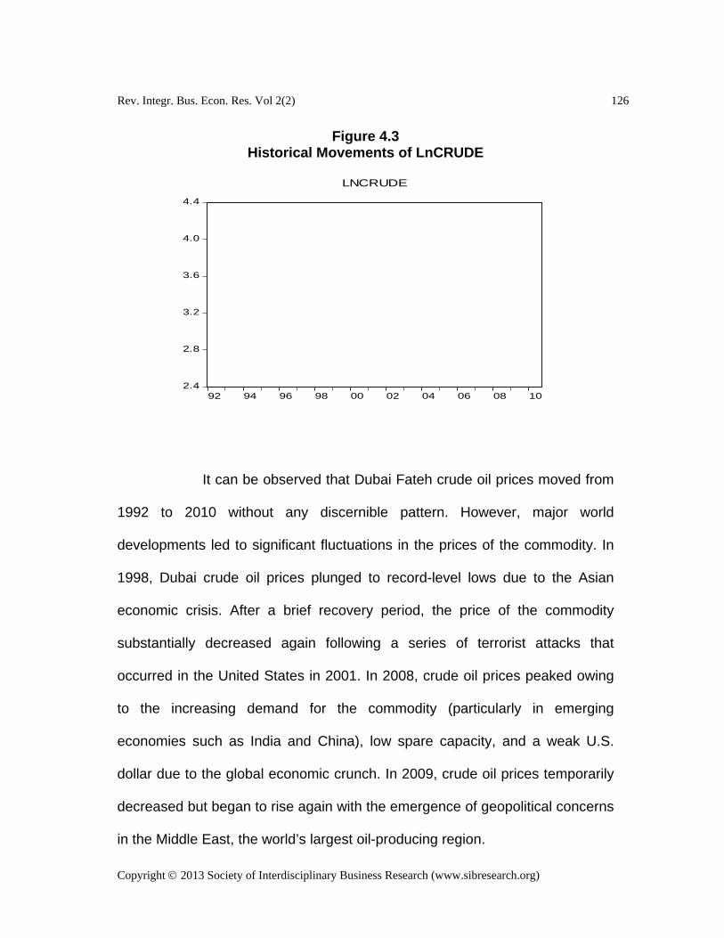
Rev. Integr. Bus. Econ. Res. Vol 2(2) 126
Copyright 2013 Society of Interdisciplinary Business Research (www.sibresearch.org)
2.4
2.8
3.2
3.6
4.0
4.4
92 94 96 98 00 02 04 06 08 10
LNCRUDE
Figure 4.3 Historical Movements of LnCRUDE
It can be observed that Dubai Fateh crude oil prices moved from
1992 to 2010 without any discernible pattern. However, major world
developments led to significant fluctuations in the prices of the commodity. In
1998, Dubai crude oil prices plunged to record-level lows due to the Asian
economic crisis. After a brief recovery period, the price of the commodity
substantially decreased again following a series of terrorist attacks that
occurred in the United States in 2001. In 2008, crude oil prices peaked owing
to the increasing demand for the commodity (particularly in emerging
economies such as India and China), low spare capacity, and a weak U.S.
dollar due to the global economic crunch. In 2009, crude oil prices temporarily
decreased but began to rise again with the emergence of geopolitical concerns
in the Middle East, the world’s largest oil-producing region.
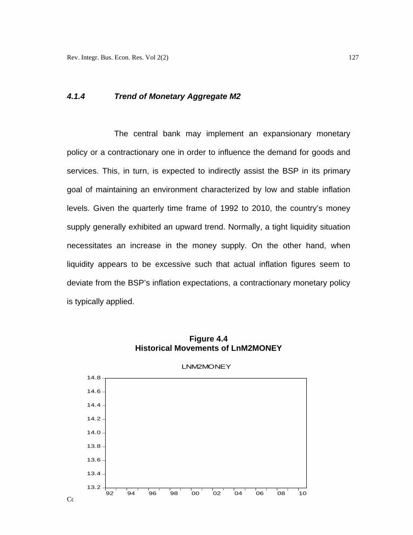
Rev. Integr. Bus. Econ. Res. Vol 2(2) 127
Copyright 2013 Society of Interdisciplinary Business Research (www.sibresearch.org)
13.2
13.4
13.6
13.8
14.0
14.2
14.4
14.6
14.8
92 94 96 98 00 02 04 06 08 10
LNM2MONEY
4.1.4 Trend of Monetary Aggregate M2
The central bank may implement an expansionary monetary
policy or a contractionary one in order to influence the demand for goods and
services. This, in turn, is expected to indirectly assist the BSP in its primary
goal of maintaining an environment characterized by low and stable inflation
levels. Given the quarterly time frame of 1992 to 2010, the country’s money
supply generally exhibited an upward trend. Normally, a tight liquidity situation
necessitates an increase in the money supply. On the other hand, when
liquidity appears to be excessive such that actual inflation figures seem to
deviate from the BSP’s inflation expectations, a contractionary monetary policy
is typically applied.
Figure 4.4 Historical Movements of LnM2MONEY

Rev. Integr. Bus. Econ. Res. Vol 2(2) 128
Copyright 2013 Society of Interdisciplinary Business Research (www.sibresearch.org)
Slow inflation growth resulted to a more apparent increase in the
country’s money supply level during 2006 and 2007. In 2006, inflation
averaged at 6.2 percent, lower than the 7.6 percent inflation rate recorded in
2005. The general price level declined further in 2007 as average inflation rate
was estimated at 2.8 percent.
Since the broad money supply evidently followed a trend, the
Log-Lin model was applied to determine its growth rate. Under this model, the
log of the variable is regressed against time. The regression results are
specified below:
LnM2MONEY = 13.3983 + 0.01724t
s.e. = (0.0228) (0.00051)
t = (587.758) (33.5078) r2 = 0.9382
Over the quarterly period 1992:Q1 to 2010:Q4, the monetary
aggregate M2 increased at a quarterly rate of 1.724 percent. This is roughly
equal to an annual average growth rate of 6.90 percent.
4.2 Testing for Stationarity
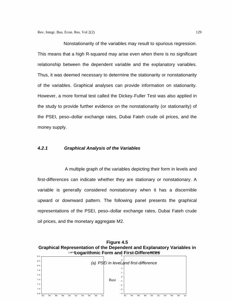
Rev. Integr. Bus. Econ. Res. Vol 2(2) 129
Copyright 2013 Society of Interdisciplinary Business Research (www.sibresearch.org)
-.4
-.3
-.2
-.1
.0
.1
.2
.3
.4
.5
92 94 96 98 00 02 04 06 08 10
DIFPSEI
6.8
7.0
7.2
7.4
7.6
7.8
8.0
8.2
8.4
92 94 96 98 00 02 04 06 08 10
LNPSEI
Nonstationarity of the variables may result to spurious regression.
This means that a high R-squared may arise even when there is no significant
relationship between the dependent variable and the explanatory variables.
Thus, it was deemed necessary to determine the stationarity or nonstationarity
of the variables. Graphical analyses can provide information on stationarity.
However, a more formal test called the Dickey–Fuller Test was also applied in
the study to provide further evidence on the nonstationarity (or stationarity) of
the PSEI, peso–dollar exchange rates, Dubai Fateh crude oil prices, and the
money supply.
4.2.1 Graphical Analysis of the Variables
A multiple graph of the variables depicting their form in levels and
first-differences can indicate whether they are stationary or nonstationary. A
variable is generally considered nonstationary when it has a discernible
upward or downward pattern. The following panel presents the graphical
representations of the PSEI, peso–dollar exchange rates, Dubai Fateh crude
oil prices, and the monetary aggregate M2.
Figure 4.5 Graphical Representation of the Dependent and Explanatory Variables in
Logarithmic Form and First-Differences
(a) PSEi in level and first-difference
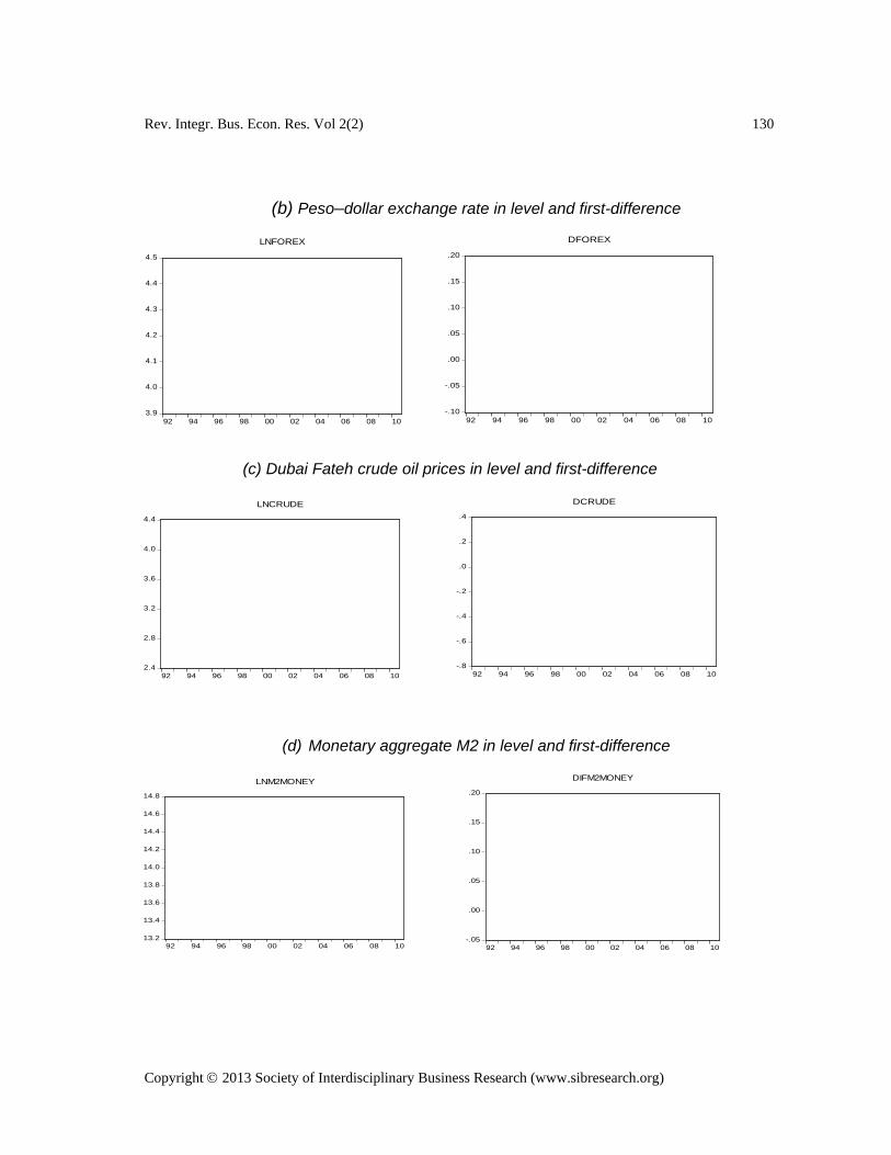
Rev. Integr. Bus. Econ. Res. Vol 2(2) 130
Copyright 2013 Society of Interdisciplinary Business Research (www.sibresearch.org)
13.2
13.4
13.6
13.8
14.0
14.2
14.4
14.6
14.8
92 94 96 98 00 02 04 06 08 10
LNM2MONEY
2.4
2.8
3.2
3.6
4.0
4.4
92 94 96 98 00 02 04 06 08 10
LNCRUDE
-.8
-.6
-.4
-.2
.0
.2
.4
92 94 96 98 00 02 04 06 08 10
DCRUDE
-.05
.00
.05
.10
.15
.20
92 94 96 98 00 02 04 06 08 10
DIFM2MONEY
3.9
4.0
4.1
4.2
4.3
4.4
4.5
92 94 96 98 00 02 04 06 08 10
LNFOREX
-.10
-.05
.00
.05
.10
.15
.20
92 94 96 98 00 02 04 06 08 10
DFOREX
(b) Peso–dollar exchange rate in level and first-difference
(c) Dubai Fateh crude oil prices in level and first-difference
(d) Monetary aggregate M2 in level and first-difference

Rev. Integr. Bus. Econ. Res. Vol 2(2) 131
Copyright 2013 Society of Interdisciplinary Business Research (www.sibresearch.org)
An apparent upward trend has been observed in the graph of
monetary aggregate M2. Meanwhile, the graphs of the variables in their first-
differenced forms indicated that the series are stationary. To further prove the
nonstationarity of the variables, a more formal test known as the Dickey–Fuller
Test was utilized.
4.2.2 Unit Root Tests
As stated in the previous section, graphical representations may
provide information on the stationarity of the variables. However, a formal test
in the form of the Dickey–Fuller Test or the ADF Test may more precisely
detect stationarity or nonstationarity. Under both tests, the null hypothesis is
that the series is nonstationary. Note, however, that the results of the Dickey–
Fuller Test are valid only when the error terms are serially uncorrelated.
Otherwise, the ADF Test should be applied (Danao, 2002).
A Durbin–Watson statistic that is approximately equivalent to 2.0
is indicative of the absence of serial correlation. In this paper, the application of
the ADF Test generated results that showed the presence of serial correlation,
thereby necessitating the use of the ADF Test. The outcome of the ADF Test
on all the four variables in their logarithmic forms and first-differences has
been summarized in the following table:

Rev. Integr. Bus. Econ. Res. Vol 2(2) 132
Copyright 2013 Society of Interdisciplinary Business Research (www.sibresearch.org)
Table 4.1 Summary of Augmented Dickey–Fuller Test Results
Variables in Levels
Variable
With Intercept With Trend and Intercept
t-Statistic Critical Value (5%) Probability t-Statistic Critical
Value (5%) Probability
LnPSEI -1.445372 -2.90122 0.5555 -1.544109 -3.471693 0.8052 LnFOREX -1.400336 -2.90122 0.5777 -1.113273 -3.471693 0.9195 LnCRUDE -1.756582 -2.90122 0.3990 -3.279494 -3.471693 0.0777 LnM2MONEY -1.074336 -2.90122 0.7219 -2.077353 -3.471693 0.5495
First-Differenced Variables
Variable With Intercept With Trend and Intercept
t-Statistic Critical Value (5%) Probability t-Statistic Critical
Value (5%) Probability
LnPSEI -6.020749 -2.901779 0.0000 -5.993283 -3.472558 0.0000 LnFOREX -4.903876 -2.90179 0.0001 -5.053009 -3.472558 0.0005 LnCRUDE -7.002439 -2.901779 0.0000 -7.074544 -3.472558 0.0000 LnM2MONEY -6.317897 -2.901779 0.0000 -6.389813 -3.472558 0.0000
The application of the ADF Test on the natural logarithm of the
variables showed that the t-statistics are lower than their corresponding critical
values at the 5.0 percent significance level. This led to the acceptance of the
null hypothesis that each of the variables has a unit root. Applying the ADF
Test on the first-differenced variables, whether the intercept or the trend and
intercept were included, yielded t-statistics that are greater than the critical
value at the 5.0 percent significance level. Therefore, the unit test results
indicated stationarity of all the variables at first-difference. While the variables
were proven to be nonstationary at levels, they were integrated of the same
order, I(1), that is, the variables have synchronized movements. On this basis,
the data were regressed in their levels form.
Rev. Integr. Bus. Econ. Res. Vol 2(2) 133
Copyright 2013 Society of Interdisciplinary Business Research (www.sibresearch.org)
4.3 Verification of the Validity of the Model using the Philippine
Stock Market
A number of existing studies made an attempt to link the stock
market to a myriad of economic factors. Some of these common economic
indicators include the GDP, inflation, and government deficits/surpluses. A
large portion of the stock market performance literature has focused on the
markets of developed countries such as the United States and members of the
European Union. The availability of such studies possibly contributed to the
sustained growth of the stock markets in these industrialized nations.
On the other hand, fewer studies were devoted to the stock
markets of developing economies such as the Philippines. The model, which
relates foreign exchange rates, crude oil prices, and money supply to stock
market performance, has also been utilized in several existing foreign literature.
However, these variables were not taken altogether, but each of them has
been used along with other usual economic indicators such as the GDP and
government budget deficits. The lack of domestic and foreign studies devoted
to the possible effects of oil price movements, monetary shocks, and foreign
exchange rates on the stock markets of developing countries served as an

Rev. Integr. Bus. Econ. Res. Vol 2(2) 134
Copyright 2013 Society of Interdisciplinary Business Research (www.sibresearch.org)
impetus for applying relevant statistical and econometric procedures on the
specified variables using the Philippine stock market.
4.3.1 Specification of the Regression Equation
Initially, the regression equation is specified as:
(4.3.1.1) LnPSEI = b0+b1LnFOREX+b2LnCRUDE+b3LnM2MONEY
The initial regression results that were based on equation (4.3.1.1) are
specified in the following table.
Table 4.2 Initial Regression Results
Dependent Variable: LNPSEI Method: Least Squares Date: 07/29/11 Time: 09:00 Sample: 1992Q1 2010Q4 Included observations: 76
Coefficient Std. Error t-Statistic Prob. C 8.928916 0.999255 8.935571 0.0000
LNFOREX -1.705534 0.161462 -10.56310 0.0000 LNCRUDE 0.101343 0.079138 1.280589 0.2044 LNMONEY 0.395120 0.084377 4.682783 0.0000
R-squared 0.671682 Mean dependent var 7.635339
Adjusted R-squared 0.658002 S.D. dependent var 0.371912 S.E. of regression 0.217496 Akaike info criterion -0.162073 Sum squared resid 3.405938 Schwarz criterion -0.039403 Log likelihood 10.15876 Hannan-Quinn criter. -0.113048 F-statistic 49.09983 Durbin–Watson stat 0.529922 Prob(F-statistic) 0.000000
Rev. Integr. Bus. Econ. Res. Vol 2(2) 135
Copyright 2013 Society of Interdisciplinary Business Research (www.sibresearch.org)
The initial regression output has provided evidence of a positive
first-order serial correlation given a very low (close to 0) Durbin–Watson
statistic at 0.529922. The incorporation of AR(1) in the equation has improved
the Durbin–Watson statistic as it grew closer to 2.0 at 1.797751 [see Appendix
for the regression results with AR(1) in the model]. Meanwhile, the null
hypothesis of no serial correlation was not rejected based on the critical values
of the Durbin–Watson statistic using n=76 and k’=3 where dL and dU is 1.54673
and 1.71043, respectively. For the Jarque–Bera Test, the JB statistic of
6.419404 has a p-value of 0.040369. Since the level of significance is 5.0
percent and 0.05 is greater than the p-value (0.040369), the null hypothesis of
the normality of the residuals has been rejected. The regression results also
showed the presence of heteroskedasticity since the p-value of the Obs*R-
squared is lower than the 5.0 percent level of significance. Moreover, there has
been a specification error problem because according to Ramsey’s RESET
results, the computed F-statistic is 0.740088, lower than the critical F at the 5.0
percent significance level (F3,72) of 2.73.
With the specification error problem and expectations that the
stock market is driven by market perceptions from its previous performance, as
well as the delayed effects of the independent variables, the lagged values of
LnPSEI and the explanatory variables LnFOREX, LnCRUDE, and
LnM2MONEY were utilized as additional regressors. The revised specification
Rev. Integr. Bus. Econ. Res. Vol 2(2) 136
Copyright 2013 Society of Interdisciplinary Business Research (www.sibresearch.org)
has been based on the optimal number of lags that were determined through
the AIC. The robustness of the revised regression equation has also been
tested for validity according to the assumptions of the classical linear
regression model.
4.3.1.1 Optimal Lag Length
The previous performance of the Philippine stock market
may have an impact on the current value of the PSEI. Moreover, peso–
dollar exchange rates, crude oil prices, and the money supply may have
delayed effects on stock market performance. Hence, the lagged values
of the PSEI and the current as well as the previous values of the peso–
dollar exchange rates, crude oil prices, and money supply were
incorporated as explanatory variables in the model.
However, the number of lags to be included should be
selected based on a criteria and theoretical knowledge. In this case, the
AIC was used to determine the optimal lag length. The results of the
AIC have shown that 4 is the optimal lag length for the model. Thus,
four-quarter lags of the PSEI, FOREX, CRUDE, and M2MONEY were
used as regressors, in addition to the current values of the original
explanatory variables. Note that when using the AIC, the optimal lag is

Rev. Integr. Bus. Econ. Res. Vol 2(2) 137
Copyright 2013 Society of Interdisciplinary Business Research (www.sibresearch.org)
chosen based on the number with the lowest AIC value. The higher the
lags, say 10 to 14 quarters, the lower the value of the AIC. However, in
theory, it does not appear realistic to state that the values of the given
explanatory variables two to three years ago still continue to affect the
PSEI.
Table 4.3
Determination of the Optimal Lag Length Number of Lags AIC SC R2 HQ
0 -0.16207 -0.03940 0.67168 -0.11305
1 -0.92005 -0.67286 0.85828 -0.82135
2 -0.92884 -0.55521 0.852714 -0.77979
3 -0.93832 -0.4363 0.889224 -0.73826
4 -0.94194 -0.30954 0.900543 -0.69018
5 -0.82329 -0.05844 0.900684 -0.51914
4.3.2 Multiple Regression Results
The possibility of obtaining spurious regression results was
eliminated given the presence of a cointegrating vector as indicated in the
results of the Johansen Cointegration Procedure. The validity of the model
using the Philippine stock market was estimated through the Ordinary Least
Squares (OLS) method. Over the period 1992:Q1 to 2010:Q4, OLS estimation
in equation form was stated as:
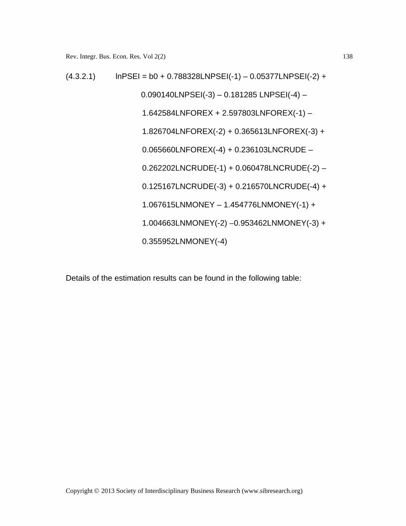
Rev. Integr. Bus. Econ. Res. Vol 2(2) 138
Copyright 2013 Society of Interdisciplinary Business Research (www.sibresearch.org)
(4.3.2.1) lnPSEI = b0 + 0.788328LNPSEI(-1) – 0.05377LNPSEI(-2) +
0.090140LNPSEI(-3) – 0.181285 LNPSEI(-4) –
1.642584LNFOREX + 2.597803LNFOREX(-1) –
1.826704LNFOREX(-2) + 0.365613LNFOREX(-3) +
0.065660LNFOREX(-4) + 0.236103LNCRUDE –
0.262202LNCRUDE(-1) + 0.060478LNCRUDE(-2) –
0.125167LNCRUDE(-3) + 0.216570LNCRUDE(-4) +
1.067615LNMONEY – 1.454776LNMONEY(-1) +
1.004663LNMONEY(-2) –0.953462LNMONEY(-3) +
0.355952LNMONEY(-4)
Details of the estimation results can be found in the following table:
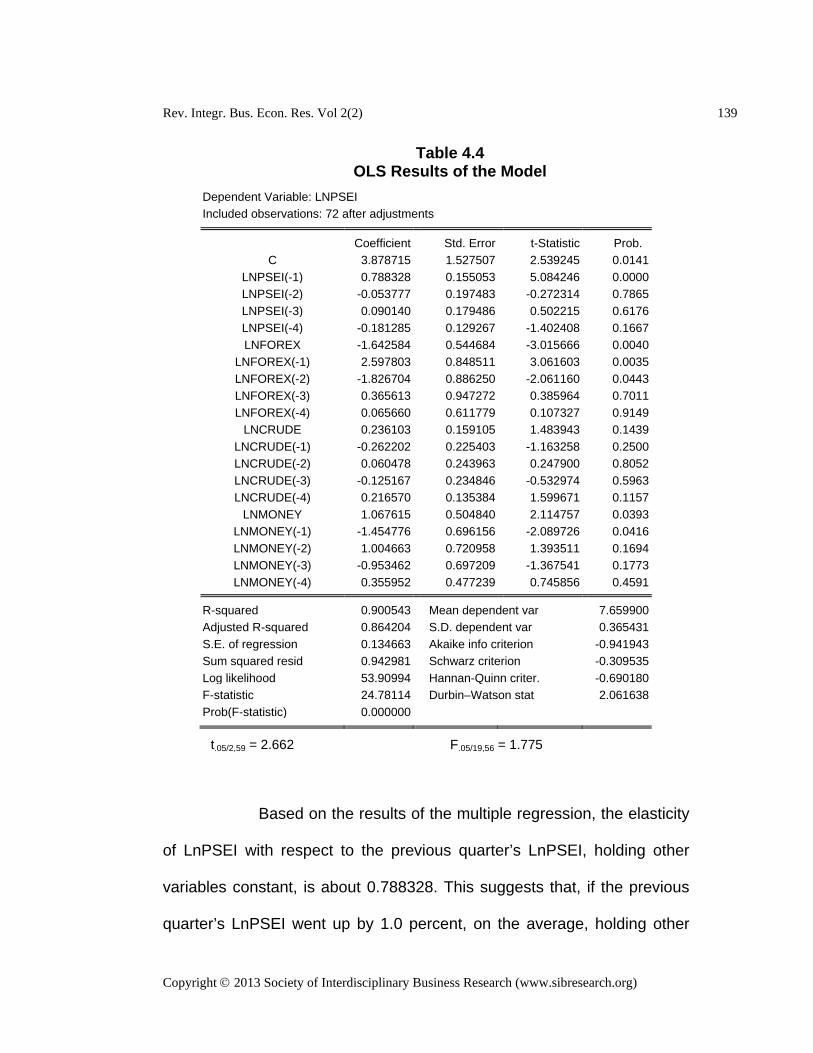
Rev. Integr. Bus. Econ. Res. Vol 2(2) 139
Copyright 2013 Society of Interdisciplinary Business Research (www.sibresearch.org)
Table 4.4 OLS Results of the Model
t.05/2,59 = 2.662 F.05/19,56 = 1.775
Based on the results of the multiple regression, the elasticity
of LnPSEI with respect to the previous quarter’s LnPSEI, holding other
variables constant, is about 0.788328. This suggests that, if the previous
quarter’s LnPSEI went up by 1.0 percent, on the average, holding other
Dependent Variable: LNPSEI Included observations: 72 after adjustments
Coefficient Std. Error t-Statistic Prob.
C 3.878715 1.527507 2.539245 0.0141 LNPSEI(-1) 0.788328 0.155053 5.084246 0.0000 LNPSEI(-2) -0.053777 0.197483 -0.272314 0.7865 LNPSEI(-3) 0.090140 0.179486 0.502215 0.6176 LNPSEI(-4) -0.181285 0.129267 -1.402408 0.1667 LNFOREX -1.642584 0.544684 -3.015666 0.0040
LNFOREX(-1) 2.597803 0.848511 3.061603 0.0035 LNFOREX(-2) -1.826704 0.886250 -2.061160 0.0443 LNFOREX(-3) 0.365613 0.947272 0.385964 0.7011 LNFOREX(-4) 0.065660 0.611779 0.107327 0.9149
LNCRUDE 0.236103 0.159105 1.483943 0.1439 LNCRUDE(-1) -0.262202 0.225403 -1.163258 0.2500 LNCRUDE(-2) 0.060478 0.243963 0.247900 0.8052 LNCRUDE(-3) -0.125167 0.234846 -0.532974 0.5963 LNCRUDE(-4) 0.216570 0.135384 1.599671 0.1157
LNMONEY 1.067615 0.504840 2.114757 0.0393 LNMONEY(-1) -1.454776 0.696156 -2.089726 0.0416 LNMONEY(-2) 1.004663 0.720958 1.393511 0.1694 LNMONEY(-3) -0.953462 0.697209 -1.367541 0.1773 LNMONEY(-4) 0.355952 0.477239 0.745856 0.4591
R-squared 0.900543 Mean dependent var 7.659900 Adjusted R-squared 0.864204 S.D. dependent var 0.365431 S.E. of regression 0.134663 Akaike info criterion -0.941943 Sum squared resid 0.942981 Schwarz criterion -0.309535 Log likelihood 53.90994 Hannan-Quinn criter. -0.690180 F-statistic 24.78114 Durbin–Watson stat 2.061638 Prob(F-statistic) 0.000000

Rev. Integr. Bus. Econ. Res. Vol 2(2) 140
Copyright 2013 Society of Interdisciplinary Business Research (www.sibresearch.org)
variables constant, the current value of LnPSEI will increase by
approximately 0.788328 percent. The responsiveness of the current
LnPSEI to the previous quarter’s change in the LnPSEI can be said to be
inelastic since it is less than one. The elasticity coefficient of LnPSEI can
be described as statistically significant since its t-statistic (5.084246)
exceeded the critical value of t.05/2,59 (2.662), leading to the rejection of the
null hypothesis. The LnPSEI lagged by two, three, and four quarters were
found to be insignificant given its corresponding p-values that exceeded
the 5.0 percent significance level.
Meanwhile, the coefficients of LnFOREX and its lagged
values showed that they have a significant and stronger impact on the
LnPSEI compared to the other explanatory variables in the model. The
coefficient of -1.642584 for LnFOREX means that, holding all the other
variables constant, a 1.0 percent increase in the current peso–dollar
exchange rate will contribute to a decrease in the LnPSEI by 1.642584
percent. For LnFOREX lagged by one quarter, a percent increase in the
LnFOREX will result to a 2.597803 percent increase in the LnPSEI,
holding the other variables constant. Note that the previous quarter’s
average peso–dollar exchange rate has a more pronounced impact on the
LnPSEI. This is representative of the lasting effect of the exchange rate on
the performance of the stock market. When lagged by two quarters,
Rev. Integr. Bus. Econ. Res. Vol 2(2) 141
Copyright 2013 Society of Interdisciplinary Business Research (www.sibresearch.org)
LnFOREX appeared to have a diminished impact on the stock market as
compared to the LnFOREX lagged by only one quarter. Specifically, a 1.0
percent increase in the LnFOREX lagged by two quarters will result to a
decrease in the LnPSEI by 1.826704 percent, holding all the other
variables constant. Finally, with p-values of 0.7011 and 0.9149, LnFOREX
lagged by three and four quarters, respectively, has been proven to be
insignificant.
Dubai Fateh crude oil price changes were shown to have an
insignificant impact on the PSEI. Current and lagged values of Dubai
Fateh crude oil prices have corresponding p-values that are greater than
the 5.0 percent significance level.
Meanwhile, changes in the money supply were found to
have a significant influence on the performance of the stock market, albeit
weaker compared to the effect of the peso–dollar exchange rates. Holding
all the other variables constant, a 1.0 percent increase in the broad money
supply will lead to a 1.067615 percent increase in the LnPSEI. Meanwhile,
a 1.0 percent increase in the broad money supply (lagged by one quarter)
will yield to a decrease in the LnPSEI by 1.454776 percent. Finally, two to
four quarter lags in the broad money supply were considered insignificant
based on the p-values generated by the multiple regression. Note that

Rev. Integr. Bus. Econ. Res. Vol 2(2) 142
Copyright 2013 Society of Interdisciplinary Business Research (www.sibresearch.org)
prior to running the multiple regression, the interest rate variable using the
90-day Treasury bill yield was used as a predictor variable. However,
initial regression results showed that this variable is statistically
insignificant.
To recapitulate, the variation in LnPSEI, as a result of the
changes in the current LnFOREX, and LnFOREX lagged by one and two
quarters have been observed to be highly significant at the 5.0 percent
significance level, holding the other variables constant. The t-statistics of
LnFOREX (-3.015666) exceeded the critical value of t.05/2,59 (2.662), thus
rejecting the null hypothesis. Meanwhile, holding the other variables
constant, the absolute values of the t-statistics of LnFOREX lagged by one
quarter (3.061603) and two quarters (-2.061160) were higher than the
critical value. For these variables, there has been very little risk of
rejecting the null hypothesis erroneously. In other words, the t-statistic
results led to the conclusion that β5, β6, and β7 are significantly different
from zero at the 5.0 percent level of significance.
Except for the coefficients of LnPSEI(-1), LnFOREX,
LnFOREX(-1), LnFOREX(-2), LnM2MONEY, and LnM2MONEY(-1), the
coefficients of the other explanatory variables were not significantly
different from zero as denoted by their corresponding p-values that are

Rev. Integr. Bus. Econ. Res. Vol 2(2) 143
Copyright 2013 Society of Interdisciplinary Business Research (www.sibresearch.org)
higher than the chosen level of significance of 5.0 percent. Moreover, the
t-statistics of these variables are lower than the critical value of t.05/2,59
(2.662).
The R2 value of 0.900543 means that about 90.05 percent of
the variation in the LnPSEI is explained by the past values of LnPSEI itself
and the current and lagged values of LnFOREX, LnCRUDE, and
LnM2MONEY. Since the R2 itself may not be an accurate prediction of
how much of the variation in the stock market performance is explained by
the model, the adjusted R2 was also reported. Taking into account the
number of explanatory variables, 86.42 percent of the variation in the
LnPSEI is explained by the regression model. Despite a lower adjusted R2,
it can still be said that a substantial proportion of the total variation in the
performance of the Philippine stock market is explained by the regression
model.
The regression model appeared to be highly significant
based on the result of the F-test. As indicated in Table 4.4, the F-statistic
of 24.78114 greatly exceeded the critical F(19, 56), which is 1.775. Therefore,
the null hypothesis stating that the explanatory variables, taken together,
have no significant effect on the performance of the Philippine stock
market was rejected. Moreover, the sample regression line fitted the data

Rev. Integr. Bus. Econ. Res. Vol 2(2) 144
Copyright 2013 Society of Interdisciplinary Business Research (www.sibresearch.org)
-.4
-.2
.0
.2
.4
6.8
7.2
7.6
8.0
8.4
8.8
94 96 98 00 02 04 06 08 10
Residual Actual Fitted
very well. This has been graphically presented in Figure 4.6, which plots
the actual data and the fitted data, as well as the residual or the difference
between the actual and fitted values of the model.
Figure 4.6
Actual, Fitted, Residual Graph
Rev. Integr. Bus. Econ. Res. Vol 2(2) 145
Copyright 2013 Society of Interdisciplinary Business Research (www.sibresearch.org)
4.3.3 Classical Linear Regression Model Assumptions
The OLS method was used to estimate the parameters of
the model. The method follows the Gauss–Markov Theorem stating that
“given the assumptions of the classical linear regression model, the least-
square estimators, in the class of unbiased linear estimators, have
minimum variance, that is, they are the best linear unbiased estimators”
(Gujarati, 2003). If the regression model failed the assumptions of the
classical linear regression model, then the βs are not the best linear
unbiased estimators.
4.3.3.1 Normality of Residuals: The Jarque–Bera Test
Among the assumptions of the classical linear
regression is the normality of the residuals. When the residuals are
non-normal, the least-square estimators are not normally distributed
in normal samples (Danao, 2005). This invalidates the confidence
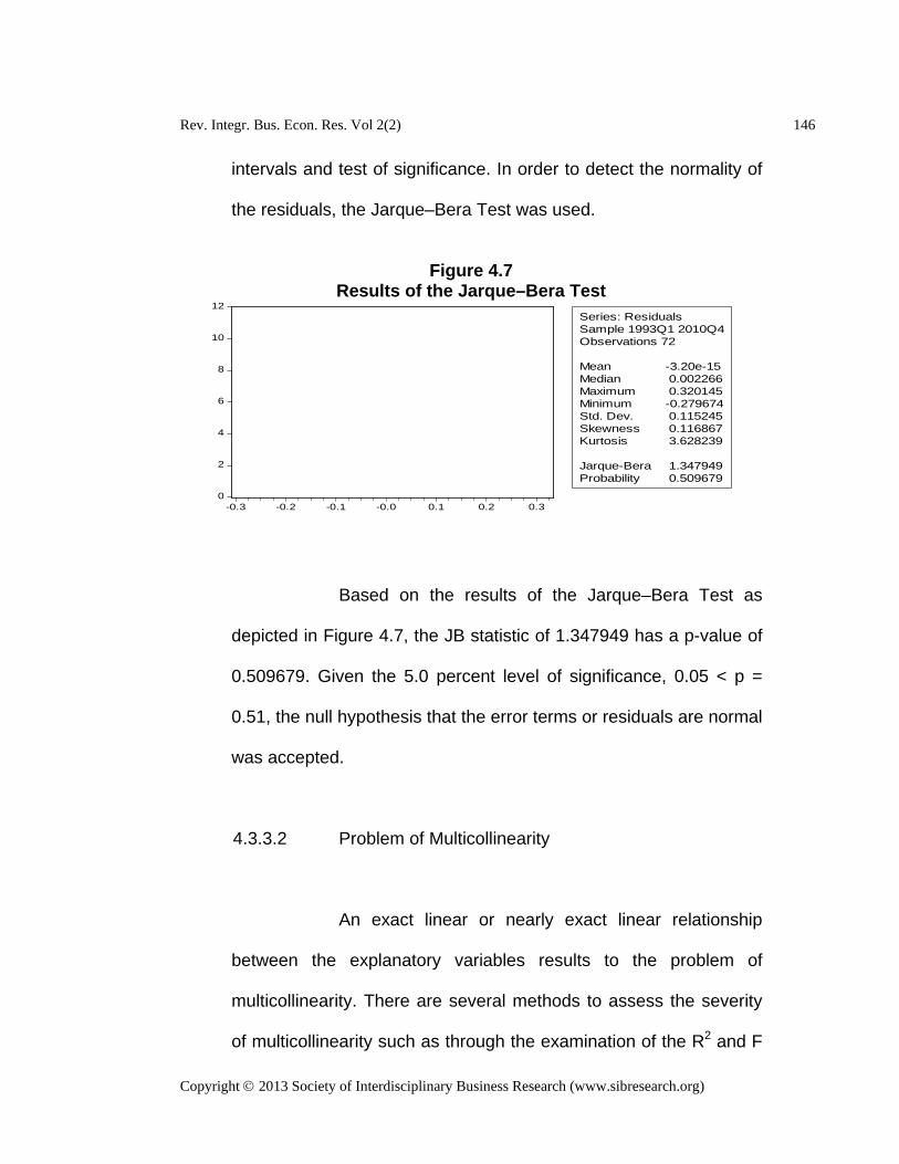
Rev. Integr. Bus. Econ. Res. Vol 2(2) 146
Copyright 2013 Society of Interdisciplinary Business Research (www.sibresearch.org)
0
2
4
6
8
10
12
-0.3 -0.2 -0.1 -0.0 0.1 0.2 0.3
Series: ResidualsSample 1993Q1 2010Q4Observations 72
Mean -3.20e-15Median 0.002266Maximum 0.320145Minimum -0.279674Std. Dev. 0.115245Skewness 0.116867Kurtosis 3.628239
Jarque-Bera 1.347949Probability 0.509679
intervals and test of significance. In order to detect the normality of
the residuals, the Jarque–Bera Test was used.
Figure 4.7
Results of the Jarque–Bera Test
Based on the results of the Jarque–Bera Test as
depicted in Figure 4.7, the JB statistic of 1.347949 has a p-value of
0.509679. Given the 5.0 percent level of significance, 0.05 < p =
0.51, the null hypothesis that the error terms or residuals are normal
was accepted.
4.3.3.2 Problem of Multicollinearity
An exact linear or nearly exact linear relationship
between the explanatory variables results to the problem of
multicollinearity. There are several methods to assess the severity
of multicollinearity such as through the examination of the R2 and F

Rev. Integr. Bus. Econ. Res. Vol 2(2) 147
Copyright 2013 Society of Interdisciplinary Business Research (www.sibresearch.org)
ratios, correlation matrix, Klein’s rule of thumb, and computing for
the Variance Inflation Factor (VIF).
One of the common symptoms of multicollinearity is
the presence of a very high R2 and insignificant t-ratios. In this case,
the R2 of 0.900543 can be considered high. Moreover, some of the
t-ratios of the parameters are insignificant except for the parameters
β1, β5, β6, β7, β15, and β16 at the 5.0 percent level of significance.
Based on these given information, it is inconclusive if the degree of
multicollinearity can be regarded as high. This inconclusiveness
necessitated the application of the other methods for testing the
severity of multicollinearity.
Based on the pair-wise correlations of the regressors,
the degree of multicollinearity appeared to be acceptable since the
correlations are not high. Note, however, that the pair-wise
correlations of the variables may be an adequate but not a
necessary condition for the existence of a strong multicollinearity.
According to Gujarati (2003), the correlation coefficients between
the regressors may be considered high once it exceeds 0.80. In this
case, none of the correlation coefficients exceeded the 0.80 value.
Table 4.5

Rev. Integr. Bus. Econ. Res. Vol 2(2) 148
Copyright 2013 Society of Interdisciplinary Business Research (www.sibresearch.org)
Correlation Matrix
Another method for testing the severity of
multicollinearity is through the examination of the VIF. The VIF is an
estimate of the increase in the variance of an estimated coefficient
due to multicollinearity (Danao, 2005). High VIFs are indicative of a
multicollinearity problem. The rule of thumb is that multicollinearity
is not a serious problem when no VIF is greater than 10.
Table 4.6 Variance Inflation Factors of the Variables
Variable Variance Inflation Factor
LnFOREX 1.219570 LnCRUDE 1.593796 LnMONEY 1.743475
The above table presents the VIFs of each of the
explanatory variables. Since none of the VIFs are larger than 10,
then the degree of multicollinearity was, again, deemed acceptable.
4.3.3.3 Test for Heteroskedasticity – White’s Test
LNCRUDE LNFOREX LNMONEY
1.00000 -0.08040 0.55228 -0.08040 1.00000 0.30292 0.55228 0.30292 1.00000
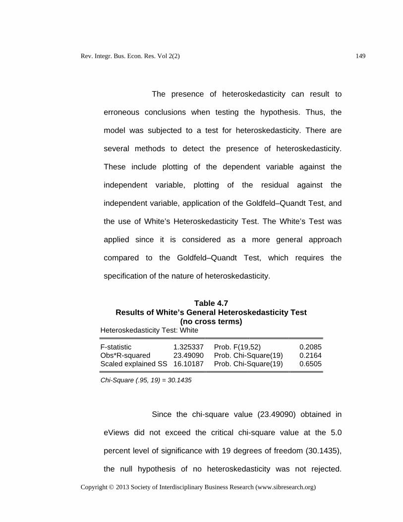
Rev. Integr. Bus. Econ. Res. Vol 2(2) 149
Copyright 2013 Society of Interdisciplinary Business Research (www.sibresearch.org)
The presence of heteroskedasticity can result to
erroneous conclusions when testing the hypothesis. Thus, the
model was subjected to a test for heteroskedasticity. There are
several methods to detect the presence of heteroskedasticity.
These include plotting of the dependent variable against the
independent variable, plotting of the residual against the
independent variable, application of the Goldfeld–Quandt Test, and
the use of White’s Heteroskedasticity Test. The White’s Test was
applied since it is considered as a more general approach
compared to the Goldfeld–Quandt Test, which requires the
specification of the nature of heteroskedasticity.
Table 4.7
Results of White’s General Heteroskedasticity Test (no cross terms)
Heteroskedasticity Test: White F-statistic 1.325337 Prob. F(19,52) 0.2085
Obs*R-squared 23.49090 Prob. Chi-Square(19) 0.2164 Scaled explained SS 16.10187 Prob. Chi-Square(19) 0.6505
Chi-Square (.95, 19) = 30.1435
Since the chi-square value (23.49090) obtained in
eViews did not exceed the critical chi-square value at the 5.0
percent level of significance with 19 degrees of freedom (30.1435),
the null hypothesis of no heteroskedasticity was not rejected.

Rev. Integr. Bus. Econ. Res. Vol 2(2) 150
Copyright 2013 Society of Interdisciplinary Business Research (www.sibresearch.org)
Moreover, the p-value of the Obs*R-squared (0.2164) is greater
than the 5.0 percent significance level.
4.3.3.4 Test for Heteroskedasticity – ARCH Test
As a supplement to White’s General
Heteroskedasticity Test and as a means to determine the possible
presence of volatility clustering among the time series variables, the
Autoregressive Conditional Heteroskedasticity (ARCH) Test was
used. As defined by Gujarati (2003), volatility clustering is a
phenomenon in which the time series data exhibit wide swings for a
given period followed by periods of relative calmness. Knowledge
of volatility clustering is primarily important since the presence of
these substantial fluctuations makes planning and decision-making
difficult.
Table 4.8
Results of Autoregressive Conditional Heteroskedasticity Test Heteroskedasticity Test: ARCH
F-statistic 1.206177 Prob. F(1,69) 0.2759
Obs*R-squared 1.219815 Prob. Chi-Square(1) 0.2694
Test Equation: Dependent Variable: RESID^2 Method: Least Squares Date: 08/10/11 Time: 09:57 Sample (adjusted): 1993Q2 2010Q4 Included observations: 71 after adjustments
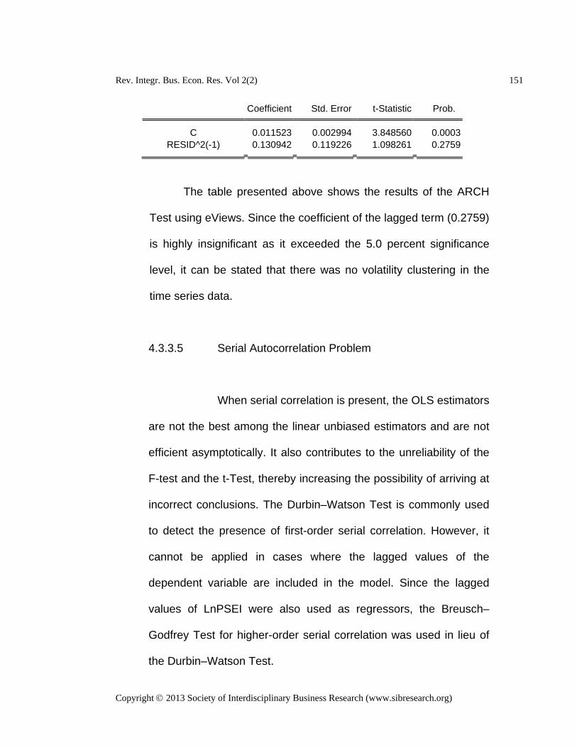
Rev. Integr. Bus. Econ. Res. Vol 2(2) 151
Copyright 2013 Society of Interdisciplinary Business Research (www.sibresearch.org)
Coefficient Std. Error t-Statistic Prob. C 0.011523 0.002994 3.848560 0.0003
RESID^2(-1) 0.130942 0.119226 1.098261 0.2759
The table presented above shows the results of the ARCH
Test using eViews. Since the coefficient of the lagged term (0.2759)
is highly insignificant as it exceeded the 5.0 percent significance
level, it can be stated that there was no volatility clustering in the
time series data.
4.3.3.5 Serial Autocorrelation Problem
When serial correlation is present, the OLS estimators
are not the best among the linear unbiased estimators and are not
efficient asymptotically. It also contributes to the unreliability of the
F-test and the t-Test, thereby increasing the possibility of arriving at
incorrect conclusions. The Durbin–Watson Test is commonly used
to detect the presence of first-order serial correlation. However, it
cannot be applied in cases where the lagged values of the
dependent variable are included in the model. Since the lagged
values of LnPSEI were also used as regressors, the Breusch–
Godfrey Test for higher-order serial correlation was used in lieu of
the Durbin–Watson Test.
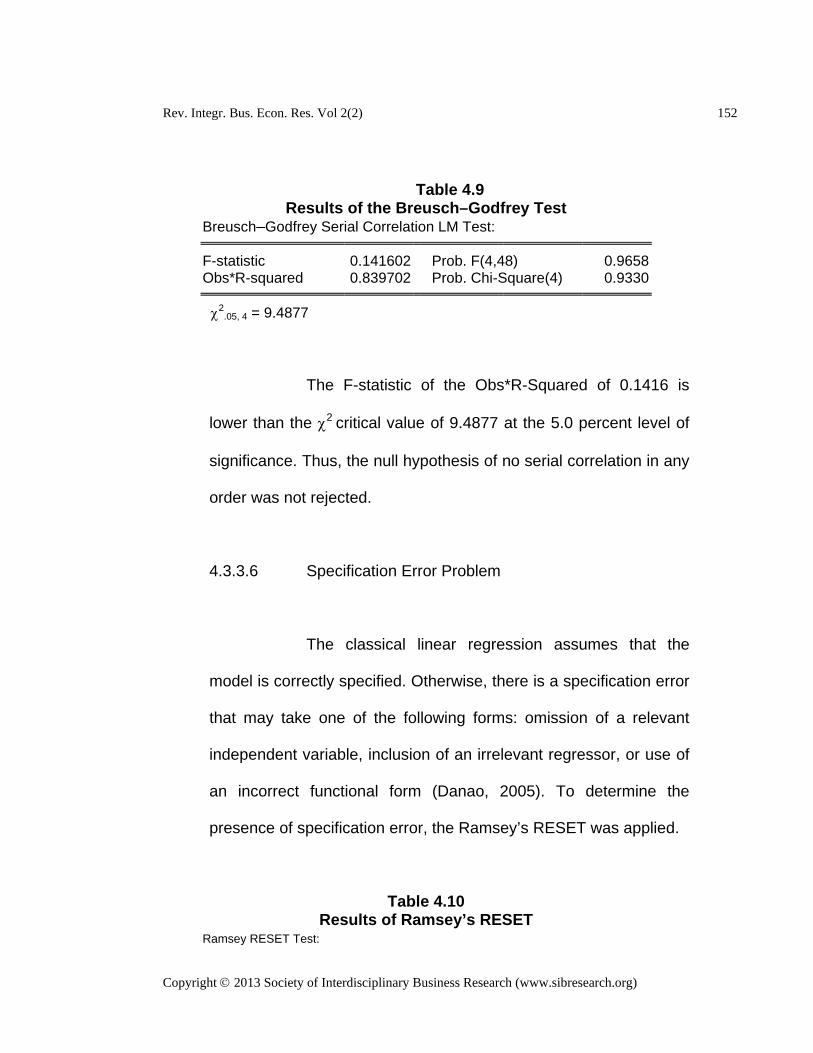
Rev. Integr. Bus. Econ. Res. Vol 2(2) 152
Copyright 2013 Society of Interdisciplinary Business Research (www.sibresearch.org)
Table 4.9 Results of the Breusch–Godfrey Test
Breusch–Godfrey Serial Correlation LM Test: F-statistic 0.141602 Prob. F(4,48) 0.9658
Obs*R-squared 0.839702 Prob. Chi-Square(4) 0.9330 χ2
.05, 4 = 9.4877
The F-statistic of the Obs*R-Squared of 0.1416 is
lower than the χ2 critical value of 9.4877 at the 5.0 percent level of
significance. Thus, the null hypothesis of no serial correlation in any
order was not rejected.
4.3.3.6 Specification Error Problem
The classical linear regression assumes that the
model is correctly specified. Otherwise, there is a specification error
that may take one of the following forms: omission of a relevant
independent variable, inclusion of an irrelevant regressor, or use of
an incorrect functional form (Danao, 2005). To determine the
presence of specification error, the Ramsey’s RESET was applied.
Table 4.10 Results of Ramsey’s RESET
Ramsey RESET Test:

Rev. Integr. Bus. Econ. Res. Vol 2(2) 153
Copyright 2013 Society of Interdisciplinary Business Research (www.sibresearch.org)
F-statistic 0.733045 Prob. F(1,51) 0.3959
Log likelihood ratio 1.027521 Prob. Chi-Square(1) 0.3107
The results of the Ramsey’s RESET indicate that
there was no specification error in the model. The computed F-
statistic of 0.7330 did not exceed the critical F-statistic of 1.775.
Therefore, the null hypothesis that the model is not misspecified
was accepted. Moreover, with a p-value of 0.3959, the null
hypothesis of no specification error in the model can be rejected at
39.59 percent, but not at a lower significance level such as 5.0
percent.
4.4 Test for the Presence of Structural Change
Structural changes in the relationship between LnPSEI and
the independent variables LnFOREX, LnCRUDE, and LnM2MONEY and
their lagged values may occur given a long quarterly time frame covering
1992 to 2010. Such structural changes may come from a number of
factors such as geopolitical, social, and economic. The structural stability
of the model has to be established so that the parameters of the
coefficients would be the same between different time periods. Thus, the

Rev. Integr. Bus. Econ. Res. Vol 2(2) 154
Copyright 2013 Society of Interdisciplinary Business Research (www.sibresearch.org)
model can be utilized as a reliable basis for forecasting and policy
formulation.
To formally determine whether structural changes
occurred in the model, the Chow Breakpoint Test was employed. This was
done by dividing the sample quarterly period from 1992 to 2010 into two
periods. The breakpoint 2001:Q2 divided the data into sub-periods
1992:Q4 to 2001:Q1 and 2001:Q2 to 2010:Q4.
Table 4.11 Results of the Chow Breakpoint Test
Chow Breakpoint Test: 2001Q2 Null Hypothesis: No breaks at specified breakpoints
F-statistic 1.360896 Prob. F(20,32) 0.2131
Log likelihood ratio 44.31515 Prob. Chi-Square(20) 0.0014 Wald Statistic 27.21792 Prob. Chi-Square(20) 0.1292
The outcome of the Chow Breakpoint Test showed that the
p-value of the F-statistic (0.2131) is higher than the chosen level of
significance (0.05). Therefore, the null hypothesis stating that there is no
structural instability was accepted. In other words, the parameters of the
model remain the same throughout the period 1992 to 2010.
4.5 Testing for Cointegration – Johansen Procedure

Rev. Integr. Bus. Econ. Res. Vol 2(2) 155
Copyright 2013 Society of Interdisciplinary Business Research (www.sibresearch.org)
In order to investigate the possible long-term relationship
between the PSEI and the explanatory variables peso–dollar exchange
rates, crude oil prices, and money supply, a cointegration test was used.
Specifically, the Johansen Cointegration Methodology was applied. Note
that other cointegration tests are available such as the Engle-Granger
Two-Step Approach. However, the Engle-Granger method is normally
strong when using only one or two explanatory variables. Given three
explanatory variables in the research, a more powerful test known as the
Johansen Cointegration Procedure was chosen.
Aside from its ability to determine long-term equilibrium
relationships, the cointegration test may also provide information on the
possibility of obtaining spurious regression results. When the regressors
are integrated of the first order I(1) and are not cointegrated, then spurious
regression may arise.
Under the Johansen Procedure, two types of tests for the
cointegration rank (r) can be used: the Trace Test and the Lambda (λ)
Max Test. In order to perform the Johansen test, the following
assumptions were applied: (Option 2) intercept (no trend) in CE – no
intercept in VAR; (Option 3) intercept (no trend) in CE and test VAR; and

Rev. Integr. Bus. Econ. Res. Vol 2(2) 156
Copyright 2013 Society of Interdisciplinary Business Research (www.sibresearch.org)
(Option 4) intercept and trend in CE – no trend in VAR. Of these three
models, Option 2 has been considered as the most restrictive. To select
the most appropriate model, a sequential approach known as the Dickey–
Pantula Principle was used. The number of lags for the Johansen
Cointegration Test was set to three, as specified by the AIC.
4.5.1 Trace Statistic Test
The Trace Test of the Johansen Procedure has the following
hypotheses:
Ho: The number of cointegrating vectors ≤ r
Ha: The number of cointegrating vectors > r
The following table presents the results of the Trace Statistic
Test, with critical values at 5.0 percent. Based on the Dickey–Pantula
principle, the most appropriate model is Option 2 (Intercept (no trend) in
CE – no intercept in VAR). For comparison purposes, the Trace Statistic
Test results using Options 3 and 4 were also summarized in the following
table.
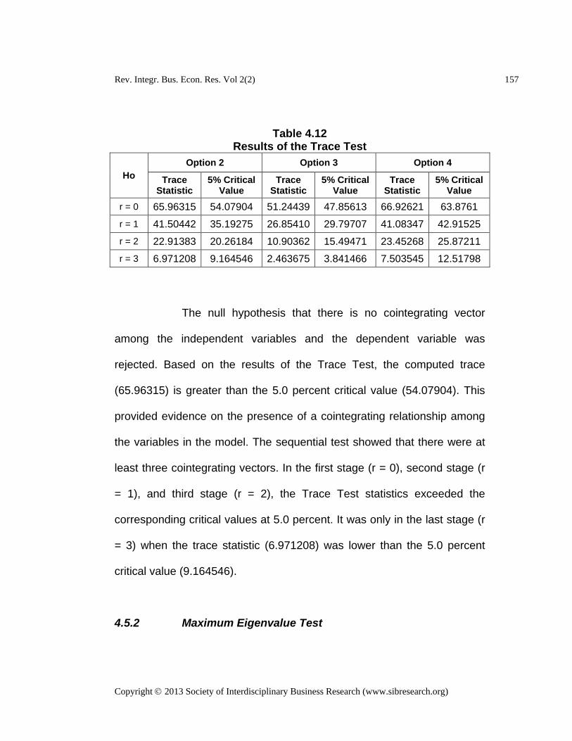
Rev. Integr. Bus. Econ. Res. Vol 2(2) 157
Copyright 2013 Society of Interdisciplinary Business Research (www.sibresearch.org)
Table 4.12 Results of the Trace Test
Ho Option 2 Option 3 Option 4
Trace Statistic
5% Critical Value
Trace Statistic
5% Critical Value
Trace Statistic
5% Critical Value
r = 0 65.96315 54.07904 51.24439 47.85613 66.92621 63.8761 r = 1 41.50442 35.19275 26.85410 29.79707 41.08347 42.91525 r = 2 22.91383 20.26184 10.90362 15.49471 23.45268 25.87211 r = 3 6.971208 9.164546 2.463675 3.841466 7.503545 12.51798
The null hypothesis that there is no cointegrating vector
among the independent variables and the dependent variable was
rejected. Based on the results of the Trace Test, the computed trace
(65.96315) is greater than the 5.0 percent critical value (54.07904). This
provided evidence on the presence of a cointegrating relationship among
the variables in the model. The sequential test showed that there were at
least three cointegrating vectors. In the first stage (r = 0), second stage (r
= 1), and third stage (r = 2), the Trace Test statistics exceeded the
corresponding critical values at 5.0 percent. It was only in the last stage (r
= 3) when the trace statistic (6.971208) was lower than the 5.0 percent
critical value (9.164546).
4.5.2 Maximum Eigenvalue Test
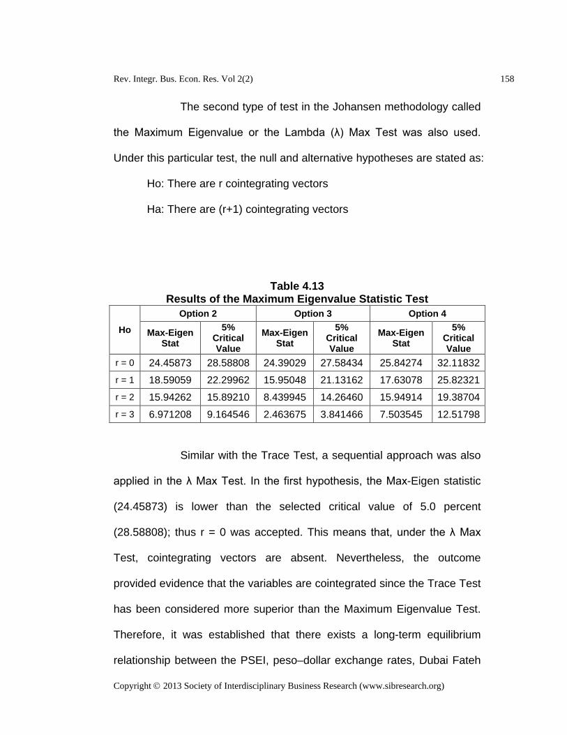
Rev. Integr. Bus. Econ. Res. Vol 2(2) 158
Copyright 2013 Society of Interdisciplinary Business Research (www.sibresearch.org)
The second type of test in the Johansen methodology called
the Maximum Eigenvalue or the Lambda (λ) Max Test was also used.
Under this particular test, the null and alternative hypotheses are stated as:
Ho: There are r cointegrating vectors
Ha: There are (r+1) cointegrating vectors
Table 4.13 Results of the Maximum Eigenvalue Statistic Test
Ho
Option 2 Option 3 Option 4
Max-Eigen Stat
5% Critical Value
Max-Eigen Stat
5% Critical Value
Max-Eigen Stat
5% Critical Value
r = 0 24.45873 28.58808 24.39029 27.58434 25.84274 32.11832 r = 1 18.59059 22.29962 15.95048 21.13162 17.63078 25.82321 r = 2 15.94262 15.89210 8.439945 14.26460 15.94914 19.38704 r = 3 6.971208 9.164546 2.463675 3.841466 7.503545 12.51798
Similar with the Trace Test, a sequential approach was also
applied in the λ Max Test. In the first hypothesis, the Max-Eigen statistic
(24.45873) is lower than the selected critical value of 5.0 percent
(28.58808); thus r = 0 was accepted. This means that, under the λ Max
Test, cointegrating vectors are absent. Nevertheless, the outcome
provided evidence that the variables are cointegrated since the Trace Test
has been considered more superior than the Maximum Eigenvalue Test.
Therefore, it was established that there exists a long-term equilibrium
relationship between the PSEI, peso–dollar exchange rates, Dubai Fateh

Rev. Integr. Bus. Econ. Res. Vol 2(2) 159
Copyright 2013 Society of Interdisciplinary Business Research (www.sibresearch.org)
crude oil prices, broad money supply, and their lagged values. On this
basis, the possibility that the regression results are spurious was further
eliminated. Therefore, the model can be estimated and tested for validity.
4.6 Granger Causality Test
As emphasized by Gujarati (2003), regression analysis
pertains to the dependence of one variable on other variables, but it does
not refer to causation or the direction of influence. In order to prove the
direction of causality among the variables, the Granger Causality Test was
used. The concept of Granger Causality states that if variable X Granger-
causes Y, then X contains information that can be useful in forecasting Y,
beyond the information included in the past values of Y alone. As
determined by the AIC, the optimal number of lags is two. Since the
variables were found to be cointegrated, the Vector Error Correction was
used instead of the Vector Autoregression. A summary of the Granger
Causality Test results was presented in Table 4.14. The full outcome of
the procedure including its details can be reviewed in the appendix section
of the paper (please refer to Appendix 22).

Rev. Integr. Bus. Econ. Res. Vol 2(2) 160
Copyright 2013 Society of Interdisciplinary Business Research (www.sibresearch.org)
Table 4.14 Results of the Granger Causality Test
Causality Probability Values
LNFOREX to LNPSEI 0.0157 LNCRUDE to LNPSEI 0.2945 LNMONEY to LNPSEI 0.4427 LNPSEI to LNFOREX 0.0564 LNPSEI to LNCRUDE 0.2244 LNPSEI to LNMONEY 0.8818
Based on the probability values specified in Table 4.14, the
variable LnFOREX Granger-causes LnPSEI. This means that the previous
values of the peso–dollar exchange rates contain information that can be
useful in forecasting the future values of the PSEI. This outcome provided
valuable support to the results of the regression analysis wherein a
relationship between LnPSEI and LnFOREX was established.
The absence of causality between the variables LnCRUDE
and LnPSEI further supported the multiple regression result that Dubai
Fateh crude oil price changes do not have a significant influence on the
performance of the Philippine stock market. Finally, the results also
showed that LnM2MONEY does not Granger-cause LnPSEI. Note that
even if the current and one period-lagged values of LnM2MONEY were
found to have a significant relationship with the LnPSEI based on the

Rev. Integr. Bus. Econ. Res. Vol 2(2) 161
Copyright 2013 Society of Interdisciplinary Business Research (www.sibresearch.org)
multiple regression analysis, the absence of causality from LnM2MONEY
to LnPSEI does not contradict the regression outcome. From a causal
point of view, the values of money supply in the previous quarters, say two
to four quarters ago, may not contain information that can be used to
forecast the future values of PSEI. However, in a shorter period (e.g.,
current quarter), previous quarter changes in the money supply may
contribute to the movements in the PSEI.
CHAPTER 5
SUMMARY, CONCLUSIONS, AND RECOMMENDATIONS
This chapter presents the summary of the research and the
conclusions that were derived from the results of the econometric tools
applied in the study. Moreover, it specifies the recommendations that were
based on the empirical results discussed in the preceding chapters. The
findings outlined in this study hope to serve as an informative contribution
to the existing literature concerning stock markets, exchange rates, crude
oil prices, and money supply. It also aims to provide relevant information

Rev. Integr. Bus. Econ. Res. Vol 2(2) 162
Copyright 2013 Society of Interdisciplinary Business Research (www.sibresearch.org)
that can be utilized for better economic policy planning and formulation
and medium- to long-term investment decision-making.
5.1 Summary and Conclusions
Through the ADF Test, it was established that the variables
are integrated at the same order at I(1). Thus, the variables utilized were
at the levels form. Given these, the regression results are non-spurious
provided that the variables are cointegrated. Three cointegrating vectors
were found based on the results of the Trace Test of the Johansen
Cointegration Procedure. The presence of the cointegrating vectors
provided evidence that the regression results are meaningful and that a
long-term relationship exists between the dependent and explanatory
variables.
Note that the regression model includes the PSEI as the
dependent variable and the lagged values of the PSEI and the current and
lagged values of the peso–dollar exchange rates, crude oil prices, and
money supply. The optimal lag length was determined to be 4 based on
the AIC. In the case of the peso–dollar exchange rates, the current up to
two-period lags were found to exert an influence on the PSEI. Meanwhile,
the current value and one-period lag of the money supply have an effect

Rev. Integr. Bus. Econ. Res. Vol 2(2) 163
Copyright 2013 Society of Interdisciplinary Business Research (www.sibresearch.org)
on the PSEI, based on the results of the regression. Thus, it can be
generally stated that the PSE capture most of the influence of government
monetary policies and changes concerning the peso–dollar exchange
rates and money supply within the quarter and up to the first or second
quarter of its implementation.
The primary regression equation (4.3.2.1) was estimated by
means of the OLS method. The estimation provided evidence that
economic variables such as the lagged values of the PSEI, current and
several lagged values of the peso–dollar exchange rates, and money
supply have an influence on the PSEI. The signs of these variables were
also found to be in accordance with the theoretical expectations of the
model. Meanwhile, Dubai Fateh crude oil prices did not appear to have a
significant influence on the PSEI. Broadly, the model itself and several
parameters obtained were found to be statistically significant.
Specifically, a 1.0 percent increase in the previous quarter’s
PSEI, holding other variables constant, on the average, will result to an
increase in the current PSEI by less than 1.0 percent (0.788328). Thus,
the responsiveness of the PSEI to its one-quarter-lagged value is
considered inelastic. Meanwhile, the current and lagged values of the

Rev. Integr. Bus. Econ. Res. Vol 2(2) 164
Copyright 2013 Society of Interdisciplinary Business Research (www.sibresearch.org)
peso–dollar exchange rates were found to have a stronger influence on
the PSEI. A 1.0 percent increase in the peso–dollar exchange rates, on
the average, will lead to a decrease in the PSEI by 1.642584 percent,
ceteris paribus. A 1.0 percent increase in the previous quarter’s peso–
dollar exchange rates, holding other variables constant, will result to an
increase in the PSEI by 2.597803 percent, on the average. In the case of
the peso–dollar exchange rates lagged by two quarters, a 1.0 percent
increase in the particular variable will translate to a decrease in the PSEI
by 1.826704 percent, ceteris paribus.
While the PSEI itself and the current and several lagged
values of the peso–dollar exchange rates were found to influence the
PSEI, Dubai Fateh crude oil price changes do not appear to significantly
affect the dependent variable. A plausible explanation for such is that the
listed companies in the exchange, particularly those that were included in
the PSEI during the time frame considered, were not primarily affected by
crude oil price fluctuations. Energy-intensive firms included in the PSEI
may have resorted to hedging in order to protect their positions from wide
price movements. Moreover, some firms could have become more
efficient in their operations, therefore, reducing the impact of substantial
crude oil price changes.

Rev. Integr. Bus. Econ. Res. Vol 2(2) 165
Copyright 2013 Society of Interdisciplinary Business Research (www.sibresearch.org)
Finally, the current and one quarter-lagged values of the
monetary aggregate M2 were found to exert a significant influence on the
PSEI. Specifically, a 1.0 percent increase in the money supply, on the
average, will lead to an increase in the PSEI by 1.067615 percent, ceteris
paribus. When lagged by one quarter, a 1.0 percent increase in the money
supply will translate to a decrease in the PSEI by 1.454776, holding the
other variables constant. It is noteworthy that the money supply lagged by
one quarter has a slightly higher coefficient than the current money supply.
This suggests that the monetary actions by the central bank tend to have
a delayed spillover effect on the performance of the stock market.
Since the model passed the following tests, namely, Jarque–
Bera, White’s Heteroskedasticity, ARCH, Breusch–Godfrey, and
Ramsey’s RESET, it can further be concluded that the parameters of the
regression equation (4.3.2.1) were statistically reliable. The outcome of
the Chow Breakpoint Test showed that there is no structural instability;
hence, the model can be useful for policy formulation and forecasting.
The possibility of obtaining spurious regression results is
further ruled out through the Johansen Cointegration Test. The procedure
also provided evidence of a long-term equilibrium relationship between the
PSEI and the explanatory variables, namely, the peso–dollar exchange
Rev. Integr. Bus. Econ. Res. Vol 2(2) 166
Copyright 2013 Society of Interdisciplinary Business Research (www.sibresearch.org)
rates, Dubai Fateh crude oil prices, and monetary aggregate M2. The two
types of testing for the cointegration rank, the Trace Test and the Lambda
Max Test, were both used. While the Trace Test showed that there are at
least three cointegrating vectors, the Lambda Max results failed to identify
cointegrating vectors. However, since the Trace Test is theoretically
accepted to be superior compared to the Lambda Max, it was therefore
concluded that there is a long-term equilibrium relationship between the
dependent and explanatory variables.
Finally, the Granger Causality Test was employed in the
study in order to prove the direction of causality among the variables.
Given that the variables are cointegrated, as evidenced in the Johansen
Cointegration Procedure, the Vector Error Correction was used. The
results showed that LnFOREX causes LnPSEI, which means that the
previous values of peso–dollar exchange rates contain information that
can be valuable in forecasting the future values of the stock index.
Meanwhile, no causality was found between LnCRUDE and LnPSEI,
further supporting the outcome of the regression analysis wherein Dubai
Fateh crude oil prices have insignificant influence on the PSEI. The
explanatory variable LnM2MONEY also does not Granger-cause LnPSEI.
As discussed in the previous section, the absence of causality from
LnM2MONEY to LnPSEI does not oppose the results of the regression.
Rev. Integr. Bus. Econ. Res. Vol 2(2) 167
Copyright 2013 Society of Interdisciplinary Business Research (www.sibresearch.org)
The regression analysis showed that the current and one quarter-lagged
values of the monetary aggregate M2 have a statistically significant
influence on the index. However, from a causal point of view, the values of
money supply in the previous quarters, say two to four quarters ago, given
that two lags were used in the Granger Causality Test, may not contain
information that can be helpful in forecasting the future values of the index.
5.2 Recommendations
This study analyzed the potential influence of the peso–
dollar exchange rates, Dubai Fateh crude oil prices, and broad money
supply on the PSEI. It also examined the long-run relationship between
the PSEI and the given regressors and investigated on the direction of
causality among these variables. On the basis of the findings derived from
the various econometric analyses and insights gained from the review of
related literature, the following recommendations are modestly presented:
1. The Philippine government, specifically economic managers,
should continuously strive for stability in the economy. Macroeconomic
policies should not only be geared toward general economic growth. It
Rev. Integr. Bus. Econ. Res. Vol 2(2) 168
Copyright 2013 Society of Interdisciplinary Business Research (www.sibresearch.org)
should also take the necessary steps to improve consumer and investor
confidence.
a) The results of the study consistently emphasized the
important role played by the current and lagged values of the peso–
dollar exchange rates on the PSEI. On this basis, the government,
particularly the central bank, should vigilantly observe the
movements of the Philippine peso relative to the U.S. dollar (and
other foreign currencies). As the Philippines adopts a managed
floating exchange rate system, the BSP has the ability to exert
some influence on the peso–dollar exchange rates and act
correspondingly to any signs of excessive exchange rate
fluctuations that may be detrimental to the economy.
b) Changes in the Dubai Fateh crude oil prices were found to
be statistically insignificant to the performance of the stock market.
Nevertheless, the Philippine government should ensure that the
country has sufficient supply of the commodity in order to prevent
shortages that could bring about elevated inflation rates in the
future. Since, crude oil reserves are continuously depleting
resources, the use of renewable energy should also be considered.

Rev. Integr. Bus. Econ. Res. Vol 2(2) 169
Copyright 2013 Society of Interdisciplinary Business Research (www.sibresearch.org)
c) Changes in the current and one quarter-lagged values of
the broad money supply were found to exert an influence on the
PSEI. Once again, monetary authorities as represented by the BSP,
have the capacity to influence the amount of money in circulation.
The BSP should continue its stance against ‘inflationary’ pressures
in the Philippine economy. Appropriate and timely monetary
policies should be deployed once unfavorable changes in the
money supply level are projected.
2. Participants in the stock market may be short-term traders or
medium- to long-term investors. Given the exposure of the instruments to
various economic and non-economic factors, market participants are
strongly encouraged to practice diversification.
Diversification reduces the risks that come naturally when an
investor opts to “keep all the eggs in one basket”. Within his portfolio, an
investor should maintain an array of investments so that when the value of
one type of asset performs poorly, other investments can neutralize the
incurred losses. Investors may also diversify across various trading time
frames. Several stocks in the portfolio may be traded on a daily or short-
term basis, while others may be kept in a longer-term basis, say a quarter
or a year. Note that the latter trading style may reduce the frequency of

Rev. Integr. Bus. Econ. Res. Vol 2(2) 170
Copyright 2013 Society of Interdisciplinary Business Research (www.sibresearch.org)
trades, hence lower commission costs and time allocated on analysis and
trading.
3. Through collaborative efforts with the concerned government
agencies, the PSE should continue to intensify its market awareness
initiatives in order to encourage the general public to invest in the stock
market. Research and development programs should also be
implemented to further enhance the operational systems of the PSE and
make it more competitive on a global scale.
4. If feasible, the private sector should continuously offer affordable
investment products and services to the general public.
5. To assist in educating the public on the available investment
options and to encourage them to place their funds in the stock market,
the Department of Education and the Commission on Higher Education
should incorporate relevant and practical investment and finance topics in
their basic study programs. The National Government should continuously
prioritize the development of the education system in the country.
Rev. Integr. Bus. Econ. Res. Vol 2(2) 171
Copyright 2013 Society of Interdisciplinary Business Research (www.sibresearch.org)
6. The local bourse, investment firms, and government agencies
that are particularly tasked with statistical data gathering should continue
to maintain a statistical database that can be useful in research
undertakings related to finance and investments. The availability and
accuracy of these statistics can also be helpful in the decision-making
processes of the government and private entities.
7. Researchers and students who are interested in conducting a
study with a similar theme in the future may adopt other economic
variables and financial variables as explanatory variables and relate it to
stock market performance. Since stocks are primarily short-term
investments, high-frequency time series data e.g. daily, monthly may also
be utilized, if available.
8. With all humility, the researcher acknowledges the fact that this
particular research remains inadequate in terms of the needed literature
that can fully contribute to the development of the Philippine stock market.
However, this study is deemed functional as a guide toward the creation of
more sophisticated and comprehensive research undertakings that could
encourage the involvement of the public in the stock market, as well as in
the design of appropriate monetary policies by the Philippine government.
Rev. Integr. Bus. Econ. Res. Vol 2(2) 172
Copyright 2013 Society of Interdisciplinary Business Research (www.sibresearch.org)
REFERENCES
Abugri, B.A. (2008). Empirical Relationship between Macroeconomic
Volatility and Stock Returns: Evidence from Latin American Markets. International Review of Financial Analysis, 17, 2, 396-410. doi:10.1016/j.irfa.2006.09.002
Aghion, P., Bacchetta, P., Ranciere, R., and Rogoff, K. (2009). Exchange Rate Volatility and Productivity Growth: The Role of Financial Development. Journal of Monetary Economics, 56, 4, 494-513. doi:10.1016/j.jmoneco.2009.03.015
Arratibel, O., Furceri, D., Martin, R., and Zdzienicka. A. (2011). The Effect of Nominal Exchange Rate Volatility on Real Macroeconomic Performance in the CEE Countries. Economic Systems, 35, 2, 261-277. doi:10.1016/j.ecosys.2010.05.003
Azeez, A.A. and Yonezawa, Y. (2006). Macroeconomic Factors and the Empirical Content of the Arbitrage Pricing Theory in the Japanese Stock Market. Japan and the World Economy, 18, 4, 568-591. doi:10.1016/j.japwor.2005.05.001
Bachmeier, L. (2008). Monetary Policy and the Transmission of Oil Shocks. Journal of Macroeconomics, 30, 4, 1738-1755. doi:10.1016/j.jmacro.2007.11.002
Baharumshah, A.Z., Mohd, S.H., and Yol, M.A. (2009). Stock Prices and Demand for Money in China: New Evidence. Journal of International Financial Markets, Institutions, & Money, 19, 1, 171-187. doi:10.1016/j.intfin.2007.11.001
Balke, N.S. and Wynne, M.A. (2007). The Relative Price Effects of
Monetary Shocks. Journal of Macroeconomics, 29, 1, 19-36. doi:10.1016/j.jmacro.2005.04.002
Basher, S.A. and Sadorsky, P. (2006). Oil Price Risk and Emerging
Stock Markets. Global Finance Journal, 17, 2, 224-251. doi:10.1016/j.gfj.2006.04.001

Rev. Integr. Bus. Econ. Res. Vol 2(2) 173
Copyright 2013 Society of Interdisciplinary Business Research (www.sibresearch.org)
Basistha, A., and Kurov, A. (2008). Macroeconomic Cycles and the Stock Market’s Reaction to Monetary Policy. Journal of Banking & Finance, 32, 12, 2606-2616. doi:10.1016/j.bankfin.2008.05.012
Bjornland, H.C. (2009). Oil Price Shocks and Stock Market Booms in
an Oil Exporting Country. Scottish Journal of Political Economy, 56, 2, 232-254
Bodenstein, M., Erceg, C.J., and Guerrieri, L. (2010). Oil Shocks and
External Adjustment. Journal of International Economics, article in press. doi:10.1016/j.jinteco.2010.10.006
Chen, S. (2009). Oil Price Pass-through into Inflation. Energy
Economics, 31, 1, 126-133. doi:10.1016/j.eneco.2008.08.006
Chen, S. (2009). Predicting the Bear Stock Market: Macroeconomic Variables as Leading Indicators. Journal of Banking & Finance, 33, 2, 211-223. doi:10.1016/j.jbankfin.2008.07.013
Chen, S. (2010). Do Higher Oil Prices Push the Stock Market into Bear
Territory? Energy Economics, 32, 2, 490-495. doi:10.1016/j.eneco.2009.08.018
Chen, M., Kim, W.G., and Kim, H.J. (2005). The Impact of Macroeconomic and Non-Macroeconomic Forces on Hotel Stock Returns. International Journal of Hospitality Management, 24, 2, 243-258. doi:10.1016/j.ijhm.2004.06.008
Chiou, J. and Lee, Y. (2009). Jump Dynamics and Volatility: Oil and the Stock Markets. Energy, 34, 6, 788-796. doi:10.1016/j.energy.2009.02.011
Choi, K. and Hammoudeh, S. (2010). Volatility Behavior of Oil,
Industrial Commodity and Stock Markets in a Regime-switching Environment. Energy Policy, 38, 8, 4388-4399. doi:10.1016/j.enpol.2010.03.067
Cong, R., Wei, Y., Jiao, J., and Fan, Y. (2008). Relationships between
Oil Price Shocks and Stock Market: An Empirical Analysis from China. Energy Policy, 36, 9, 3544-3553. doi:10.1016/j.enpol.2008.06.006

Rev. Integr. Bus. Econ. Res. Vol 2(2) 174
Copyright 2013 Society of Interdisciplinary Business Research (www.sibresearch.org)
Cooray, A. (2010). Do Stock Markets Lead to Economic Growth? Journal of Policy Modeling, 32, 4, 448-460. doi:10.1016/j.jpolmod.2010.05.001
Diamandis, P.F. and Drakos, A.A. (2011). Financial Liberalization, Exchange Rates and Stock Prices: Exogenous Shocks in Four Latin America Countries. Journal of Policy Modeling, 33, 3, 381-394. doi:10.1016/j.jpolmod.2010.11.004
Du, D. (2006). Monetary Policy, Stock Returns, and Inflation. Journal of Economics and Business, 58, 1, 36-54. doi:10.1016/j.econbus.2005.06.003
Du, L., Yanan, H., and Wei, C. (2010). The Relationship between Oil
Price Shocks and China’s Macroeconomy: An Empirical Analysis. Energy Policy, 38, 8, 4142-4151. doi:10.1016/j.enpol.2010.03.042
Enisan, A.A. and Olufisayo, A.O. (2009). Stock Market Development
and Economic Growth: Evidence from Seven Sub Sahara African Countries. Journal of Economics and Business, 61, 2, 162-171. doi:10.1016/j.jeconbus.2008.05.001
Farka, M. (2009). The Effect of Monetary Policy Shocks on Stock Price
Accounting for Endogeneity and Omitted Variable Biases. Review of Financial Economics, 18, 1, 47-55. doi:10.1016/j.rfe.2008.05.003
Farzanegan, M.R. and Markwardt, G. (2009). The Effects of Oil Price
Shocks on the Iranian Economy. Energy Economics, 31, 1, 134-151. doi:10.1016/j.eneco.2008.09.003
Favara, G. and Giordani, P. (2009). Reconsidering the Role of Money for Output, Prices and Interest Rates, Journal of Monetary Economics, 56, 3, 419-430. doi:10.1016/j.jmoneco.2009.01.002
Fofana, I., Chitiga, M., and Mabugu, R. (2009). Oil Prices and the
South African Economy: A Macro-Meso-Micro Analysis. Energy Policy, 37, 12, 5509-5518. doi:10.1016/j.enpol.2009.08.030
Hafer, R.W., Haslag, J.H., and Jones, G. (2007). On Money and
Output: Is Money Redundant? Journal of Monetary Economics, 54, 3, 945-954. doi:10.1016/j.jmoneco.2005.06.004

Rev. Integr. Bus. Econ. Res. Vol 2(2) 175
Copyright 2013 Society of Interdisciplinary Business Research (www.sibresearch.org)
He, L.T. (2006). Variations in Effects of Monetary Policy on Stock Market Returns in the Past Four Decades. Review of Financial Economics, 15, 4, 331-349. doi:10.1016/j.rfe.2005.07.001
Heimonen, K. (2010). Money and Equity Returns in the Euro Area.
Global Finance Journal, 21, 2, 152-169. doi:10.1016/j.gfj.2010.06.003
Henriques, I. and Sadorsky, P. (2010). The Effect of Oil Price Volatility
on Strategic Investment. Energy Economics, 33, 1, 79-87. doi:10.1016/j.eneco.2010.09.001
Iwayemi, A. and Fowowe, B. (2011). Impact of Oil Price Shocks on
Selected Macroeconomic Variables in Nigeria. Energy Policy, 39, 2, 603-612. doi:10.1016/j.enpol.2010.10.033
Jammazi, R. and Aloui, C. (2010). Wavelet Decomposition and
Regime Shifts: Assessing the Effects of Crude Oil Shocks on Stock Market Returns. Energy Policy, 38, 3, 1415-1435. doi:10.1016/j.enpol.2009.11.023
Jayaraman, T.K. and Choong, C. (2009). Growth and Oil Price: A
Study of Causal Relationships in Small Pacific Island Countries. Energy Policy, 37, 6, 2182-2189. doi:10.1016/j.enpol.2009.01.025
Jbir, R. and Zouari-Ghorbel, S. (2009). Recent Oil Price Shock and
Tunisian Economy. Energy Policy, 37, 3, 1041-1051. doi:10.1016/j.enpol.2008.10.044
Jimenez-Rodriguez, R. (2008). The Impact of Oil Price Shocks:
Evidence from the Industries of Six OECD Countries. Energy Economics, 30, 6, 3095-3108. doi:10.1016/j.eneco.2008.06.002
Kasman, S., Vardar, G., and Tunc, G. (2011). The Impact of Interest Rate and Exchange Rate Volatility on Banks’ Stock Returns and Volatility: Evidence from Turkey. Economic Modelling, 28, 3, 1328-1334. doi:10.1016/j.econmod.2011.01.015
Kholodilin, K., Montanoli, A., Napolitano, O., and Siliverstovs, B.
(2009). Assessing the Impact of the ECB's Monetary Policy on the Stock Markets: A Sectoral View. Economics Letters, 105, 3, 211-213. doi:10.1016/j.econlet.2009.08.006

Rev. Integr. Bus. Econ. Res. Vol 2(2) 176
Copyright 2013 Society of Interdisciplinary Business Research (www.sibresearch.org)
Kormilitisina, A. (2011). Oil Price Shocks and the Optimality of Monetary Policy. Review of Economic Dynamics, 14, 1, 199-223. doi:10.1016/j.red.2010.11.001
Kurov, A. (2010). Investor Sentiment and the Stock Market’s Reaction to Monetary Policy. Journal of Banking & Finance, 34, 1, 139-149. doi:10.1016/j.jbankfin.2009.07.010
Lee, Y. and Chiou, J. (2011). Oil Sensitivity and its Asymmetric Impact
on the Stock Market. Energy, 36, 1, 168-174. doi:10.1016/j.energy.2010.10.057
Li, Y.D., Iscan, T.B., and Xu, K. (2010). The Impact of Monetary Policy
Shocks on Stock Prices: Evidence from Canada and the United States. Journal of International Money and Finance, 29, 5, 876-896. doi:10.1016/j.jimonfin.2010.03.008
Lim, K., Brooks, R.D., and Kim, J.H. (2008). Financial Crisis and Stock
Market Efficiency: Empirical Evidence from Asian Countries. International Review of Financial Analysis, 17, 3, 571-591. doi:10.1016/j.irfa.2007.03.001
Liu, L. and Zhang, W. (2010). A New Keynesian Model for Analysing
Monetary Policy in Mainland China. Journal of Asian Economics, 21, 6, 540-551. doi:10.1016/j.asieco.2010.07.004
Lorde, T., Jackman, M., and Thomas, C. (2009). The Macroeconomic Effects of Oil Price Fluctuations on a Small Open Oil-Producing Country: The Case of Trinidad and Tobago. Energy Policy, 37, 7, 2708-2716. doi:10.1016/j.enpol.2009.03.004
Maysami, R.C. and Koh, T.S. (2000). A Vector Error Correction Model
of the Singapore Stock Market. International Review of Economics & Finance, 9, 1, 79-96. doi:10.1016/S1059-0560(99)00042-8
Milani, F. (2009). Expectations, Learning, and the Changing
Relationship between Oil Prices and the Macroeconomy. Energy Economics, 31, 6, 827-837. doi:10.1016/j.eneco.2009.05.012
Miller, J.I. and Ratti, R.A. (2009). Crude Oil and Stock Markets: Stability, Instability, and Bubbles. Energy Economics, 31, 4, 559-568. doi:10.1016/j.eneco.2009.01.009

Rev. Integr. Bus. Econ. Res. Vol 2(2) 177
Copyright 2013 Society of Interdisciplinary Business Research (www.sibresearch.org)
Mun, K. (2007). Volatility and Correlation in International Stock Markets and the Role of Exchange Rate Fluctuations. Journal of International Financial Markets, Institutions and Money, 17, 1, 25-41. doi:10.1016/j.intfin.2005.08.006
Naccache, C. (2010). Slow Oil Shocks and the "Weakening of the Oil-
Price Macroeconomy Relationship". Energy Policy, 38, 5, 2340-2345. doi:10.1016/j.enpol.2009.12.021
Nagayasu, F. (2007). Empirical Analysis of the Exchange Rate
Channel in Japan. Journal of International Money and Finance, 26, 6, 887-904. doi:10.1016/j.jimonfin.2007.05.002
Nandha, M. and Faff, R. (2008). Does Oil Move Equity Prices? A
Global View. Energy Economics, 30, 3, 986-997. doi:10.1016/j.eneco.2007.09.003
Nandha, M. and Hammoudeh, S. (2007). Systematic Risk, and Oil
Price and Exchange Rate Sensitivities in Asia-Pacific Stock Markets. Research in International Business and Finance, 21, 2, 326-341. doi:10.1016/j.ribaf.2006.09.001
Narayan, P.K. and Narayan, S. (2010). Modelling the Impact of Oil Prices on Vietnam’s Stock Prices. Applied Energy, 87, 1, 356-361. doi:10.1016/j.apenergy.2009.05.037
Prasad, A., Narayan, P.K., and Narayan, J. (2007). Exploring the Oil Price and Real GDP Nexus for a Small Island Economy, the Fiji Islands. Energy Policy, 35, 12, 6506-6513. doi:10.1016/j.enpol.2007.07.032
Qianqian, Z. (2011). The Impact of International Oil Price Fluctuation
on China’s Economy. Energy Procedia, 5, 1360-1364. doi:10.1016/j.egypro.2011.03.235
Rafiq, S., Salim, R., and Bloch, H. (2009). Impact of Crude Oil Price
Volatility on Economic Activities: An Empirical Investigation in the Thai Economy. Resources Policy, 34, 3, 121-132. doi:10.1016/j.resourpol.2008.09.001
Rousseau, P.L. and Xiao, S. (2007). Banks, Stock Markets, and
China’s ‘Great Leap Forward’. Emerging Markets Review, 8, 3, 206-217. doi:10.1016/j.ememar.2007.05.002
Rev. Integr. Bus. Econ. Res. Vol 2(2) 178
Copyright 2013 Society of Interdisciplinary Business Research (www.sibresearch.org)
Scharler, J. (2008). Bank Lending and the Stock Market’s Response to Monetary Policy Shocks. International Review of Economics & Finance, 17, 3, 425-435. doi:10.1016/j.iref.2007.01.002
Schnabl, G. (2008). Exchange Rate Volatility and Growth in Small
Open Economies at the EMU Periphery. Economic Systems, 32, 1, 70-91. doi:10.1016/j.ecosys.2007.06.006
Tang, W., Wu, L., and Zhang, Z. (2010). Oil Price Shocks and their
Short- and Long-Term Effects on the Chinese Economy. Energy Economics, 32, 1, S3-S14. doi:10.1016/j.eneco.2010.01.002
Walid, C., Chaker, A., Masood, O., and Fry, J. (2011). Stock Market
Volatility and Exchange Rates in Emerging Countries: A Markov-state Switching Approach. Emerging Markets Review, 12, 3, 272-292. doi:10.1016/j.ememar.2011.04.003
Wongbangpo, P. and Sharma, S.C. (2002). Stock Market and Macroeconomic Fundamental Dynamic Interactions: ASEAN-5 Countries. Journal of Asian Economics, 13, 1, 27-51. doi:10.1016/S1049-0078(01)00111-7
Wu, J., Hou, H., and Cheng, S. (2010). The Dynamic Impacts of Financial Institutions on Economic Growth: Evidence from the European Union. Journal of Macroeconomics, 32, 3, 879-891. doi:10.1016/j.jmacro.2009.09.003
Yang, Y. and Chang, C. (2008). A Double-threshold GARCH Model of
Stock Market and Currency Shocks on Stock Returns. Mathematics and Computers in Simulation, 79, 3, 458-474. doi:10.1016/j.matcom.2008.01.048
Zhang, D. (2008). Oil Shock and Economic Growth in Japan: A Nonlinear Approach. Energy Economics, 30, 5, 2374-2390. doi:10.1016/j.eneco.2008.01.006
Zhang, W. (2009). China’s Monetary Policy: Quantity Versus Price Rules. Journal of Macroeconomics, 31, 3, 473-484. doi:10.1016/j.jmacro.2008.09.003
Zhao, H. (2010). Dynamic Relationship between Exchange Rate and Stock Price: Evidence from China. Research in International Business and Finance, 24, 2, 103-112. doi:10.1016/j.ribaf.2009.09.001

Rev. Integr. Bus. Econ. Res. Vol 2(2) 179
Copyright 2013 Society of Interdisciplinary Business Research (www.sibresearch.org)
Books:
Danao, R.A. (2002). Introduction to Statistics and Econometrics. The University of the Philippines Press: Quezon City, Philippines
Danao, R.A. (2005). Introduction to Statistics and Econometrics.
University of the Philippines Press: Quezon City, Philippines
Gujarati, D. (2003). Basic Econometrics. McGraw-Hill Higher Education: New York
Mishkin, F.S. (2007). Monetary Policy Strategy. MIT Press: Massachusetts
Ramanathan, R. (2002). Introductory Econometrics with Applications (5th ed.). South-Western/Thomson Learning: Ohio
Vinod, H.D. (2008). Hands-On Intermediate Econometrics Using R:
Templates for Extending Dozens of Practical Samples. World Scientific Publishing Co. Pte. Ltd.: Singapore
Online References:
Bangko Sentral ng Pilipinas. (2011). The Exchange Rate. Retrieved
from http://www.bsp.gov.ph/downloads/Publications/FAQs/ exchange.pdf
Bangko Sentral ng Pilipinas. (2011). The BSP and Price Stability.
Retrieved from http://www.bsp.gov.ph/downloads/Publications/ FAQs/targeting.pdf
Regional Economic Monitoring Unit, Asian Development Bank (2000).
Asia Recovery Report 2000, 2. Retrieved from http://aric.adb.org/pdf/aem/may00/May_ARR_complete.pdf
National Statistical Coordination Board. (2007). Technical Notes,
Foreign Direct Investments. Retrieved from http://www.nscb.gov.ph/technotes/fdi_tech_06Feb06.asp

Rev. Integr. Bus. Econ. Res. Vol 2(2) 180
Copyright 2013 Society of Interdisciplinary Business Research (www.sibresearch.org)
APPENDIX
Appendix 1. Summary of Reviewed Journals AUTHOR TITLE JOURNAL METHODOLOGY
1.) Abugri, B.A. (2008) Empirical Relationship between
Macroeconomic Volatility and Stock Returns: Evidence from Latin American Markets
International Review of Financial Analysis
Vector Autoregression
Global variables (MSCI world index and the 3-month T-bill yield) played a substantial role in explaining returns in all the stock markets considered.
Interest rates and exchange rates were found to have important impact on three of the four markets included.
Country-specific factors affected these markets at different degrees and significance.
2.) Aghion, P., Bacchetta , P., Ranciere, R., and Rogoff, K. (2009)
Exchange Rate Volatility and Productivity Growth:
The Role of Financial Development
Journal of Monetary
Economics
GMM Dynamic Panel Estimation
Using cross-country panel data, the authors found that excessive fluctuations in the exchange rate can negatively affect economic growth, especially in the long run.
Financial development is necessary in the linkage between the exchange rate regime choice and long-run economic growth.
3.) Arratibel, O., Furceri, D.,
Martin, R., and Zdzienicka,A. (2011)
The Effect of Nominal Exchange Rate Volatility on Real Macroeconomic Performance in the CEE
Countries
Economic Systems
Panel Estimations
Lower exchange rate volatility was linked to higher economic growth, higher stocks of foreign direct investments, higher current account deficits and excess credit.
4.) Azeez, A.A. and Yonezawa, Y. (2006)
Macroeconomic Factors and the Empirical Content
of the Arbitrage Pricing Theory in the Japanese
Stock Market
Japan and the World Economy
Multivariate Non-Linear Regression
Macroeconomic variables such as money supply, inflation, exchange rate, and industrial production have significant influences on the expected returns of Japanese stocks.
During the bubble period, the variances of the macroeconomic factors are relatively the same.
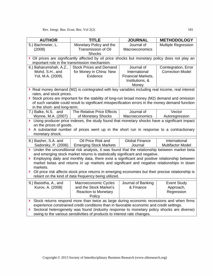
Rev. Integr. Bus. Econ. Res. Vol 2(2) 181
Copyright 2013 Society of Interdisciplinary Business Research (www.sibresearch.org)
AUTHOR TITLE JOURNAL METHODOLOGY 5.) Bachmeier, L.
(2008) Monetary Policy and the
Transmission of Oil Shocks
Journal of Macroeconomics
Multiple Regression
Oil prices are significantly affected by oil price shocks but monetary policy does not play an important role in the transmission mechanism.
6.) Baharumshah, A.Z., Mohd, S.H., and Yol, M.A. (2009).
Stock Prices and Demand for Money in China: New
Evidence
Journal of International
Financial Markets, Institutions, &
Money
Cointegration, Error Correction Model
Real money demand (M2) is cointegrated with key variables including real income, real interest rates, and stock prices.
Stock prices are important for the stability of long-run broad money (M2) demand and omission of such variable could result to significant misspecification errors in the money demand function in the short- and long-term.
7.) Balke, N.S. and Wynne, M.A. (2007)
The Relative Price Effects of Monetary Shocks
Journal of Macroeconomics
Vector Autoregression
Using producer price indexes, the study found that monetary shocks have a significant impact on the prices of goods.
A substantial number of prices went up in the short run in response to a contractionary monetary shock.
8.) Basher, S.A. and Sadorsky, P. (2006)
Oil Price Risk and Emerging Stock Markets
Global Finance Journal
International Multifactor Model
Under the unconditional risk analysis, it was found that the relationship between market beta and emerging stock market returns is statistically significant and negative.
Employing daily and monthly data, there exist a significant and positive relationship between market betas and returns in up markets and significant and negative relationships in down markets.
Oil price risk affects stock price returns in emerging economies but their precise relationship is reliant on the kind of data frequency being utilized.
9.) Basistha, A., and Kurov, A. (2008)
Macroeconomic Cycles and the Stock Market’s Reaction to Monetary
Policy
Journal of Banking & Finance
Event Study Approach, Regression
Stock returns respond more than twice as large during economic recessions and when firms experience constrained credit conditions than in favorable economic and credit settings.
Sectoral heterogeneity was found (industry response to monetary policy shocks are diverse) owing to the various sensitivities of products to interest rate changes.
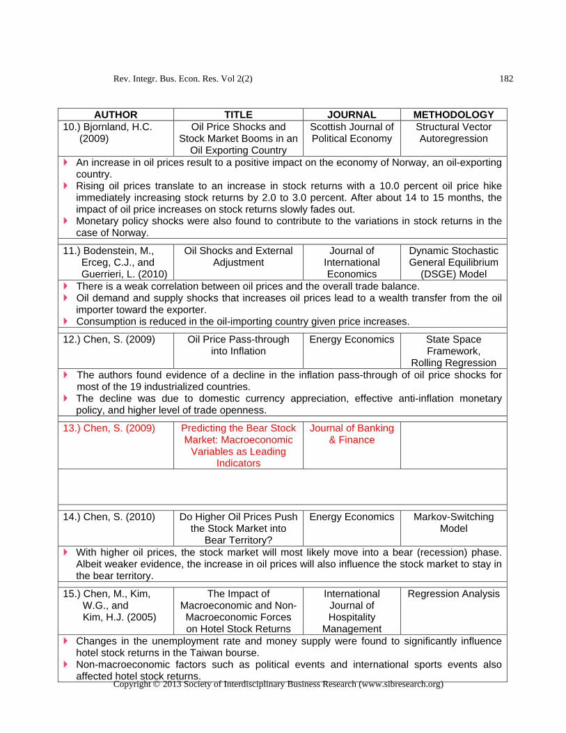
Rev. Integr. Bus. Econ. Res. Vol 2(2) 182
Copyright 2013 Society of Interdisciplinary Business Research (www.sibresearch.org)
AUTHOR TITLE JOURNAL METHODOLOGY 10.) Bjornland, H.C.
(2009) Oil Price Shocks and
Stock Market Booms in an Oil Exporting Country
Scottish Journal of Political Economy
Structural Vector Autoregression
An increase in oil prices result to a positive impact on the economy of Norway, an oil-exporting country.
Rising oil prices translate to an increase in stock returns with a 10.0 percent oil price hike immediately increasing stock returns by 2.0 to 3.0 percent. After about 14 to 15 months, the impact of oil price increases on stock returns slowly fades out.
Monetary policy shocks were also found to contribute to the variations in stock returns in the case of Norway.
11.) Bodenstein, M., Erceg, C.J., and Guerrieri, L. (2010)
Oil Shocks and External Adjustment
Journal of International Economics
Dynamic Stochastic General Equilibrium
(DSGE) Model There is a weak correlation between oil prices and the overall trade balance. Oil demand and supply shocks that increases oil prices lead to a wealth transfer from the oil
importer toward the exporter. Consumption is reduced in the oil-importing country given price increases.
12.) Chen, S. (2009) Oil Price Pass-through into Inflation
Energy Economics State Space Framework,
Rolling Regression The authors found evidence of a decline in the inflation pass-through of oil price shocks for
most of the 19 industrialized countries. The decline was due to domestic currency appreciation, effective anti-inflation monetary
policy, and higher level of trade openness.
13.) Chen, S. (2009) Predicting the Bear Stock Market: Macroeconomic
Variables as Leading Indicators
Journal of Banking & Finance
14.) Chen, S. (2010) Do Higher Oil Prices Push the Stock Market into
Bear Territory?
Energy Economics Markov-Switching Model
With higher oil prices, the stock market will most likely move into a bear (recession) phase. Albeit weaker evidence, the increase in oil prices will also influence the stock market to stay in the bear territory.
15.) Chen, M., Kim, W.G., and
Kim, H.J. (2005)
The Impact of Macroeconomic and Non-Macroeconomic Forces on Hotel Stock Returns
International Journal of Hospitality
Management
Regression Analysis
Changes in the unemployment rate and money supply were found to significantly influence hotel stock returns in the Taiwan bourse.
Non-macroeconomic factors such as political events and international sports events also affected hotel stock returns.

Rev. Integr. Bus. Econ. Res. Vol 2(2) 183
Copyright 2013 Society of Interdisciplinary Business Research (www.sibresearch.org)
AUTHOR TITLE JOURNAL METHODOLOGY 16.) Chiou, J. and Lee, Y. (2009)
Jump Dynamics and Volatility:
Oil and the Stock Markets
Energy Autoregressive Conditional Jump Intensity Model
“High fluctuations” in oil prices lead to asymmetric unexpected effects on S&P 500 returns. On the other hand, the magnitude of the impact is not the same when in an environment of “low fluctuations”.
Oil price volatility has a significant and negative effect on stock returns.
17.) Choi, K. and Hammoudeh, S. (2010)
Volatility Behavior of Oil, Industrial
Commodity and Stock Markets in a Regime-switching Environment
Energy Policy Markov-switching GARCH models:
Univariate MS Heteroskedasticity Model, Dynamic
Conditional Correlation (DCC)
Multivariate GARCH model
Commodities have different sensitivities to volatility regimes. Brent & WTI crude oils were found to be more volatility persistent over time in effect of
geopolitical crises while the S&P 500 is sensitive to both geopolitical and financial crises.
18.) Cong, R., Wei, Y., and Fan, Y. (2008)
Relationships between Oil Price Shocks and Stock
Market: An Empirical Analysis from China
Energy Policy Cointegration Test, Vector
Autoregression
Except for the manufacturing index and stock returns of some oil companies, oil price shocks do not have a statistically significant effect on stock market indices.
There is no evidence of an asymmetric impact of oil price shocks on the stock returns of oil companies.
Rise in the volatility of oil does not impact on most stock market returns but does increase returns on mining and petrochemicals index due to speculations.
The importance of oil price shocks and interest rates varies across indices.
19.) Cooray, A. (2010) Do Stock Markets Lead to Economic
Growth
Journal of Policy Modeling
Ordinary Least Squares,
GMM Estimation, Regression
Long-run economic growth is determined by human capital and stock market development policies.
Physical capital was found to have a positive effect on economic growth while population growth has a negative impact.
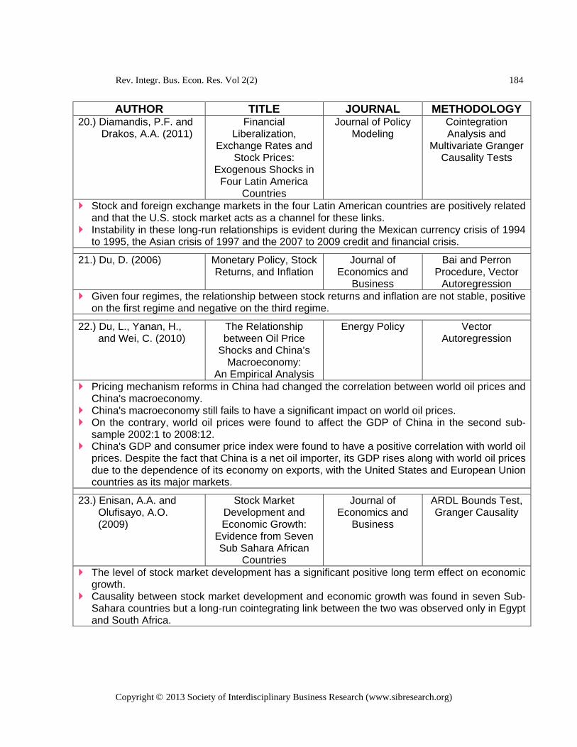
Rev. Integr. Bus. Econ. Res. Vol 2(2) 184
Copyright 2013 Society of Interdisciplinary Business Research (www.sibresearch.org)
AUTHOR TITLE JOURNAL METHODOLOGY 20.) Diamandis, P.F. and
Drakos, A.A. (2011) Financial
Liberalization, Exchange Rates and
Stock Prices: Exogenous Shocks in
Four Latin America Countries
Journal of Policy Modeling
Cointegration Analysis and
Multivariate Granger Causality Tests
Stock and foreign exchange markets in the four Latin American countries are positively related and that the U.S. stock market acts as a channel for these links.
Instability in these long-run relationships is evident during the Mexican currency crisis of 1994 to 1995, the Asian crisis of 1997 and the 2007 to 2009 credit and financial crisis.
21.) Du, D. (2006) Monetary Policy, Stock Returns, and Inflation
Journal of Economics and
Business
Bai and Perron Procedure, Vector
Autoregression Given four regimes, the relationship between stock returns and inflation are not stable, positive
on the first regime and negative on the third regime.
22.) Du, L., Yanan, H., and Wei, C. (2010)
The Relationship between Oil Price
Shocks and China’s Macroeconomy:
An Empirical Analysis
Energy Policy Vector Autoregression
Pricing mechanism reforms in China had changed the correlation between world oil prices and China's macroeconomy.
China's macroeconomy still fails to have a significant impact on world oil prices. On the contrary, world oil prices were found to affect the GDP of China in the second sub-
sample 2002:1 to 2008:12. China's GDP and consumer price index were found to have a positive correlation with world oil
prices. Despite the fact that China is a net oil importer, its GDP rises along with world oil prices due to the dependence of its economy on exports, with the United States and European Union countries as its major markets.
23.) Enisan, A.A. and Olufisayo, A.O. (2009)
Stock Market Development and Economic Growth:
Evidence from Seven Sub Sahara African
Countries
Journal of Economics and
Business
ARDL Bounds Test, Granger Causality
The level of stock market development has a significant positive long term effect on economic growth.
Causality between stock market development and economic growth was found in seven Sub-Sahara countries but a long-run cointegrating link between the two was observed only in Egypt and South Africa.

Rev. Integr. Bus. Econ. Res. Vol 2(2) 185
Copyright 2013 Society of Interdisciplinary Business Research (www.sibresearch.org)
AUTHOR TITLE JOURNAL METHODOLOGY 24.) Farka, M. (2009) The Effect of Monetary
Policy Shocks on Stock Price
Accounting for Endogeneity and Omitted Variable
Biases
Review of Financial
Economics
Regression, GARCH
The volatility effect of policy shocks by the Federal Reserve is tent-shaped, spiking during the policy announcements and falling before and after the announcements.
The level and volatility of stock returns responds asymmetrically, depending on the type of policy shocks and policy actions.
25.) Farzanegan, M.R. and Markwardt, G. (2009)
The Effects of Oil Price Shocks on the Iranian
Economy
Energy Economics Unrestricted Vector Autoregression
Positive oil price shocks were found to increase the real effective exchange rate and cause the appreciation of the rial. In turn, imports become cheaper while export prices increase.
However, inflation is not significantly affected by both positive and negative oil price shocks in Iran.
Note also that negative oil price shocks have a more pronounced effect on Iran compared to positive oil price shocks.
26.) Favara, G. and Giordani, P. (2009)
Reconsidering the Role of Money for
Output, Prices, and Interest Rates
Journal of Monetary
Economics
Vector Autoregression
Shocks to broad monetary aggregates have significant and continual impact on output, prices, and interest rates.
The outcome contradicted theoretical expectations which perceive monetary aggregates as non-substantial in the determination of the mentioned economic variables.
27.) Fofana, I., Chitiga, M., and Mabugu, R. (2009)
Oil Prices and the South African
Economy: A Macro-Meso-Micro Analysis
Energy Policy Input-Output Model with Household
Survey
Sustained high oil prices mostly affect the transport services and primary plastics industries in South Africa owing to larger input costs.
The varying distributional effects of high oil prices among expenditure groups or households are largely explained by the impact of the price increases on transport services.
28.) Hafer, R.W., Haslag, J.H., and Jones, G. (2007)
On Money and Output: Is Money Redundant
Journal of Monetary
Economics
Regression Analysis
Money supply is not considered redundant. Specifically, movements in real monetary aggregate M2 are found to have a significant impact on the output gap, independent of the real federal funds rate.
This provides evidence that the real interest rate is not the only meaningful indicator of monetary policy.
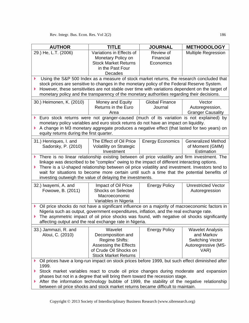
Rev. Integr. Bus. Econ. Res. Vol 2(2) 186
Copyright 2013 Society of Interdisciplinary Business Research (www.sibresearch.org)
AUTHOR TITLE JOURNAL METHODOLOGY 29.) He, L.T. (2006) Variations in Effects of
Monetary Policy on Stock Market Returns
in the Past Four Decades
Review of Financial
Economics
Multiple Regression
Using the S&P 500 Index as a measure of stock market returns, the research concluded that stock prices are sensitive to changes in the monetary policy of the Federal Reserve System.
However, these sensitivities are not stable over time with variations dependent on the target of monetary policy and the transparency of the monetary authorities regarding their decisions.
30.) Heimonen, K. (2010) Money and Equity Returns in the Euro
Area
Global Finance Journal
Vector Autoregression,
Granger Causality Euro stock returns were not granger-caused (much of its variation is not explained) by
monetary policy variables and euro stock returns do not have an impact on liquidity. A change in M3 monetary aggregate produces a negative effect (that lasted for two years) on
equity returns during the first quarter.
31.) Henriques, I. and Sadorsky, P. (2010)
The Effect of Oil Price Volatility on Strategic
Investment
Energy Economics Generalized Method of Moment (GMM)
Estimation There is no linear relationship existing between oil price volatility and firm investment. The
linkage was described to be "complex" owing to the impact of different interacting options. There is a U-shaped relationship between oil price volatility and investment. Investors tend to
wait for situations to become more certain until such a time that the potential benefits of investing outweigh the value of delaying the investments.
32.) Iwayemi, A. and Fowowe, B. (2011)
Impact of Oil Price Shocks on Selected
Macroeconomic Variables in Nigeria
Energy Policy Unrestricted Vector Autoregression
Oil price shocks do not have a significant influence on a majority of macroeconomic factors in Nigeria such as output, government expenditures, inflation, and the real exchange rate.
The asymmetric impact of oil price shocks was found, with negative oil shocks significantly affecting output and the real exchange rate in Nigeria.
33.) Jammazi, R. and Aloui, C. (2010)
Wavelet Decomposition and
Regime Shifts: Assessing the Effects
of Crude Oil Shocks on Stock Market Returns
Energy Policy Wavelet Analysis and Markov
Switching Vector Autoregressive (MS-
VAR)
Oil prices have a long-run impact on stock prices before 1999, but such effect diminished after 1999.
Stock market variables react to crude oil price changes during moderate and expansion phases but not in a degree that will bring them toward the recession stage.
After the information technology bubble of 1999, the stability of the negative relationship between oil price shocks and stock market returns became difficult to maintain.

Rev. Integr. Bus. Econ. Res. Vol 2(2) 187
Copyright 2013 Society of Interdisciplinary Business Research (www.sibresearch.org)
AUTHOR TITLE JOURNAL METHODOLOGY
34.) Jayaraman, T.K. and Choong, C. (2009)
Growth and Oil Price: A Study of Causal
Relationships in Small Pacific Island
Countries
Energy Policy ARDL Bounds Testing
Oil prices and GDP have a unidirectional relationship, which means that the linkage runs only from oil prices to international reserves to GDP but not otherwise.
Oil prices were found to have an inverse relationship with economic growth.
35.) Jbir, R. and Zouari-Ghorbel, S. (2009)
Recent Oil Price Shock and Tunisian
Economy
Energy Policy Vector Autoregression
The effect of oil price shocks is indirectly transmitted via government subsidy policies, represented by the budget deficit.
The impact of oil price shocks on the CPI was minimal and insignificant.
36.) Jimenez-Rodriguez, R. (2008)
The Impact of Oil Price Shocks: Evidence from
the Industries of Six OECD Countries
Energy Economics Recursively Identified Bivariate
VAR
Across four EMU countries, industrial output response to oil price shocks differ owing to industrial structure variety.
A common monetary policy should be taken with critical care among these economies since it may bring about asymmetric effects due to the diverse responses of these countries to oil price shocks.
37.) Kasman, S., Vardar, G., and Tunc, G. (2011)
The Impact of Interest Rate and Exchange
Rate Volatility on Banks’ Stock Returns
and Volatility: Evidence from Turkey
Economic Modelling OLS Method, Generalized
Autoregressive Conditional
Heteroskedasticity (GARCH)
Interest rate and exchange rate fluctuations were found to be important determinants of the volatility of conditional bank stock returns.
Changes in the interest rates and exchange rates have a negative and significant effect on the conditional bank return.
38.) Kholodilin, K., Montanoli, A., Napolitano, O., and Siliverstovs, B. (2009)
Assessing the Impact of the ECB's Monetary
Policy on the Stock Markets: A Sectoral
View
Economics Letters Heteroskedasticity- Based Estimator,
Event Study Approach
European Central Bank’s (ECB) monetary policies were found to have heterogeneous effects on sectoral indices. Not all sectors respond to monetary policy announcements.
Affected sectors respond with an index decrease to interest rate hikes. Overall, the aggregate stock market index also decreases when interest rates are adjusted upwards.

Rev. Integr. Bus. Econ. Res. Vol 2(2) 188
Copyright 2013 Society of Interdisciplinary Business Research (www.sibresearch.org)
AUTHOR TITLE JOURNAL METHODOLOGY 39.) Kormilitisina, A.
(2011) Oil Price Shocks and
the Optimality of Monetary Policy
Review of Economic Dynamics
Dynamic Stochastic General Equilibrium
Monetary policy plays an important role in the transmission of the impact of oil price shocks to the GDP.
Incorrect monetary polices could have exacerbated past recessions that followed oil price shocks.
Using monetary policy, the optimal response to an oil price shock is to raise inflation and interest rates (higher than what has been actually done by the government in response to the oil price shock).
40.) Kurov, A. (2010) Investor Sentiment and the Stock Market’s Reaction to Monetary
Policy
Journal of Banking & Finance
Markov-Switching Model,
Multiple Regression
Monetary policy shocks significantly affect investor sentiments, with the impact seen as more pronounced during bear market periods.
Stocks deemed more sensitive to changes in investor sentiments have a stronger response to monetary policy news.
Changes in the timing, even of expected monetary policy decisions, have a significant impact on investor sentiment as well as on stock prices in bear markets. Such was attributed to the possibility that changes in the timing of expected monetary policies carry essential information in bear market periods and that stock investors tend to overreact to timing shocks during these times.
41.) Lee, Y. and Chiou, J. (2011)
Oil Sensitivity and its Asymmetric Impact on
the Stock Market
Energy Markov-Regime Switching Model, ARMA-GARCH
Model, ARJI Model Oil prices have a significant negative impact on stock returns using the S&P 500 as the index. However, such asymmetric unexpected changes in oil prices only hold in a high oil fluctuation
regime. In other words, the anticipated, unexpected, and asymmetric unexpected changes in the prices of oil spot and futures do not have an effect on the S&P 500 given a low oil price fluctuation setting.

Rev. Integr. Bus. Econ. Res. Vol 2(2) 189
Copyright 2013 Society of Interdisciplinary Business Research (www.sibresearch.org)
AUTHOR TITLE JOURNAL METHODOLOGY
42.) Li, Y.D., Iscan, T.B., and Xu, K. (2010)
The Impact of Monetary Policy Shocks on Stock Prices: Evidence from
Canada and the United States
Journal of International Money and Finance
Structural Vector Autoregression
In Canada, the immediate reaction of stock prices to monetary policy shocks is described as small and brief whereas in the United States, the immediate response of U.S. stock prices is large and prolonged. Such response differences are attributed to the financial market openness of the two countries. Canada is considered as a small open economy while the United States is taken as a relatively large and closed economy.
The overall effect of the external demand shocks on Canadian stock prices is small owing to the floating exchange rate regime which served as a "protection" against the transmission of the external demand shocks to the real sector.
43.) Lim, K., Brooks, R.D., and Kim, J.H. (2008)
Financial Crisis and Stock Market Efficiency: Empirical Evidence from
Asian Countries
International Review of Financial Analysis
Rolling Bicorrelation (H-Statistic)
The 1997 Asian financial crisis was found to have an adverse effect on the stock markets of Asian countries that were included in the study.
The stock indices of these countries registered negative returns during the crisis. In terms of market efficiency, Hong Kong was observed to suffer the most among the countries considered, followed by Philippines.
For the post-crisis sub-sample, market efficiency improved in these Asian markets.
44.) Liu, L. and Zhang, W. (2010)
A New Keynesian Model for Analysing Monetary Policy in
Mainland China
Journal of Asian Economics
GMM
Given the current economic and financial market development of China, a hybrid monetary policy (interest rate and money supply) is more effective than one which uses a single instrument alone.
A severe appreciation of the renminbi may stabilize inflation risks, but may also distort the growth of the economy.
45.) Lorde, T., Jackman, M., and Thomas, C. (2009)
The Macroeconomic Effects of Oil Price Fluctuations on a
Small Open Oil-producing Country: The Case of Trinidad
and Tobago
Energy Policy Vector Autoregression
Oil prices were found to have an influence on the economy of Trinidad and Tobago. A positive oil price shock results to a decline in output in the first two years, followed by an
increasing and positive reaction to the shock. Price level and government revenues significantly responded to unexpected oil price volatility
shocks.
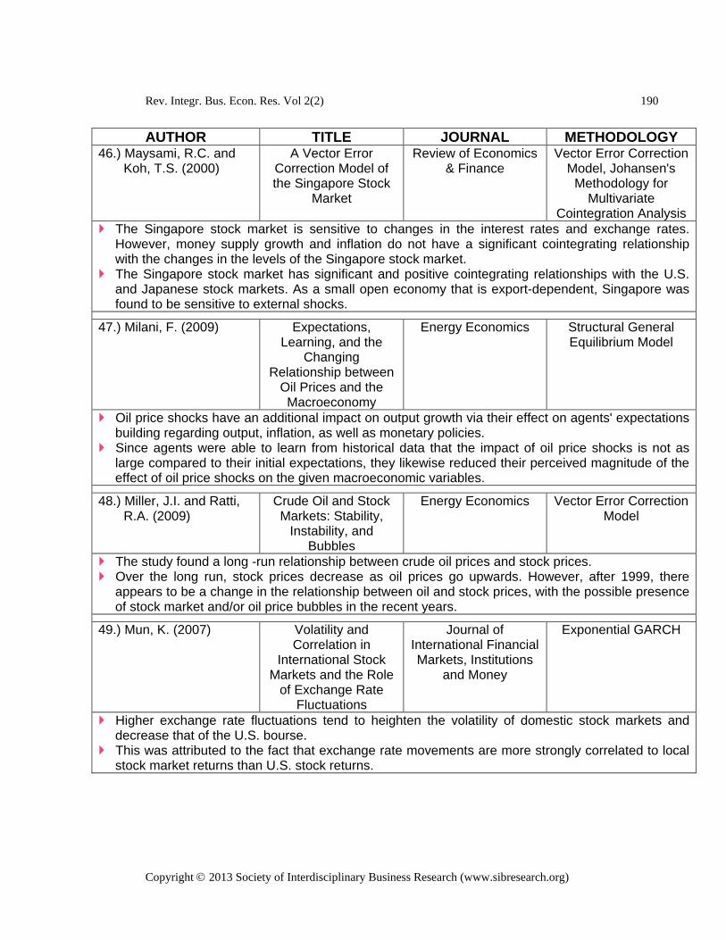
Rev. Integr. Bus. Econ. Res. Vol 2(2) 190
Copyright 2013 Society of Interdisciplinary Business Research (www.sibresearch.org)
AUTHOR TITLE JOURNAL METHODOLOGY 46.) Maysami, R.C. and
Koh, T.S. (2000) A Vector Error
Correction Model of the Singapore Stock
Market
Review of Economics & Finance
Vector Error Correction Model, Johansen's
Methodology for Multivariate
Cointegration Analysis The Singapore stock market is sensitive to changes in the interest rates and exchange rates.
However, money supply growth and inflation do not have a significant cointegrating relationship with the changes in the levels of the Singapore stock market.
The Singapore stock market has significant and positive cointegrating relationships with the U.S. and Japanese stock markets. As a small open economy that is export-dependent, Singapore was found to be sensitive to external shocks.
47.) Milani, F. (2009) Expectations, Learning, and the
Changing Relationship between
Oil Prices and the Macroeconomy
Energy Economics Structural General Equilibrium Model
Oil price shocks have an additional impact on output growth via their effect on agents' expectations building regarding output, inflation, as well as monetary policies.
Since agents were able to learn from historical data that the impact of oil price shocks is not as large compared to their initial expectations, they likewise reduced their perceived magnitude of the effect of oil price shocks on the given macroeconomic variables.
48.) Miller, J.I. and Ratti, R.A. (2009)
Crude Oil and Stock Markets: Stability,
Instability, and Bubbles
Energy Economics Vector Error Correction Model
The study found a long -run relationship between crude oil prices and stock prices. Over the long run, stock prices decrease as oil prices go upwards. However, after 1999, there
appears to be a change in the relationship between oil and stock prices, with the possible presence of stock market and/or oil price bubbles in the recent years.
49.) Mun, K. (2007) Volatility and Correlation in
International Stock Markets and the Role
of Exchange Rate Fluctuations
Journal of International Financial Markets, Institutions
and Money
Exponential GARCH
Higher exchange rate fluctuations tend to heighten the volatility of domestic stock markets and decrease that of the U.S. bourse.
This was attributed to the fact that exchange rate movements are more strongly correlated to local stock market returns than U.S. stock returns.

Rev. Integr. Bus. Econ. Res. Vol 2(2) 191
Copyright 2013 Society of Interdisciplinary Business Research (www.sibresearch.org)
AUTHOR TITLE JOURNAL METHODOLOGY 50.) Naccache, C. (2010) Slow Oil Shocks
and the "Weakening of the
Oil-Price Macroeconomy Relationship"
Energy Policy Vector Autoregression, Recursive Exclusion
Test
The weakening of the oil price-macroeconomy relationship in the recent years was attributed to the emergence of slow or non-accelerating oil price shocks during the seventies and the eighties.
These non-accelerating oil price shocks were believed to come from progressive demand shocks due to the increasing oil requirements of rapidly growing economies such as China and India.
By removing these non-accelerating oil price shocks, the study was able to restore the relationship between oil prices and the macroeconomy.
51.) Nagayasu, J. (2007) Empirical Analysis of the Exchange Rate Channel in
Japan
Journal of International Money
and Finance
Stability Tests, Markov Switching-Vector Error
Correction Model
In the case of Japan, no evidence was found to support the perception that the depreciation of the yen aided in the growth of the economy.
Therefore, the exchange rate as a transmission mechanism of monetary policy was dubbed as ineffective in removing Japan from the liquidity trap.
52.) Nandha, M. and Faff, R. (2008)
Does Oil Move Equity Prices? A
Global View
Energy Economics Standard Market Model augmented by
the oil price factor
No evidence was found for the asymmetric impact of oil prices on equity markets. Oil price shocks have a negative effect on stock market returns, except in the mining, oil, and
gas sectors. It suggested diversification involving the inclusion of assets with positive oil price sensitivity
and the utilization of oil-based derivatives.
53.) Nandha, M. and Hammoudeh, S. (2007)
Systematic Risk, and Oil Price and Exchange Rate
Sensitivities in Asia-Pacific Stock
Markets
Research in International Business and
Finance
International Factor Model
A significant but minimal relationship was found to exist between the domestic beta risk and the stock markets in China and Thailand, regardless of whether oil prices are in US dollars or in their respective domestic currencies.
Only the Philippines and South Korea were found to be sensitive to oil prices in the short run when oil is expressed in the local currency, but none of these countries were sensitive to oil price changes when using the U.S. dollar.
Oil sensitivity may vary when the oil market is categorized into "up" and "down" markets. The Philippines is seen to be oil price-sensitive whether it is in an "up" or in a "down" oil market.

Rev. Integr. Bus. Econ. Res. Vol 2(2) 192
Copyright 2013 Society of Interdisciplinary Business Research (www.sibresearch.org)
AUTHOR TITLE JOURNAL METHODOLOGY 54.) Narayan, P.K. and
Narayan, S. (2010) Modelling the
Impact of Oil Prices on Vietnam’s Stock
Prices
Applied Energy Long-run Elasticities, Error Correction Model
Stock prices in the Vietnam Stock Exchange (VN-index), oil prices, and nominal exchange rates are cointegrated (have long-run relationships).
Estimating long-run elasticities, oil prices and exchange rates have a positive influence on stock prices while for the short-run elasticities, neither of the two independent variables has a statistically significant effect on the VN-index.
55.) Prasad, A., Narayan, P.K., and Narayan, J. (2007)
Exploring the Oil Price and Real GDP
Nexus for a Small Island Economy, the Fiji Islands
Energy Policy Granger Causality, Impulse Response Function, Variance
Decomposition
The study found a positive relationship between oil prices and GDP in the case of Fiji, an oil-importing country.
The positive relationship was attributed to the possibility that the Fijian economy has not yet reached the threshold where oil prices will negatively affect output (similar to the case of developed economies).
56.) Qianqian, Z. (2011) The Impact of International Oil
Price Fluctuation on China’s Economy
Energy Procedia Cointegration, Error Correction Model
A long-run equilibrium relationship exists between oil prices and China’s output, CPI, net exports, and monetary policy.
Surging oil prices have an inverse influence on net exports and real output while it causes the CPI to increase.
Monetary authorities tend to implement tight monetary policy given the inflationary risks brought about by rising oil prices.
57.) Rafiq, S., Salim, R., and Bloch, H. (2009)
Impact of Crude Oil Price Volatility on
Economic Activities: An Empirical
Investigation in the Thai Economy
Resources Policy Vector Autoregression
A unidirectional causality running from oil price volatility toward investment, unemployment rate, interest rate, and trade balance was found.
The largest impact of oil price volatility was on investments and unemployment rate. After the financial crisis, the effect of oil price volatility was lessened but mostly affected the
budget deficit, which may be due to the introduction of the floating exchange rate regime, post-crisis.

Rev. Integr. Bus. Econ. Res. Vol 2(2) 193
Copyright 2013 Society of Interdisciplinary Business Research (www.sibresearch.org)
AUTHOR TITLE JOURNAL METHODOLOGY 58.) Rousseau, P.L. and
Xiao, S. (2007) Banks, Stock Markets, and
China’s ‘Great Leap Forward’
Emerging Markets Review
Vector Autoregression
Improvements in the size and level of sophistication in the China's banking sector have positive and significant impact on output and fixed investment.
However, developments in the stock market do not have an effect on both output and investment which may be attributed to economic activities mostly occurring outside the Chinese stock market.
59.) Scharler, J. (2008) Bank Lending and the Stock Market’s
Response to Monetary Policy
Shocks
International Review of
Economics & Finance
Limited Participation Model
Bank-dependent firms were found to respond slightly stronger to monetary policy shocks (interest rate changes) compared to bond-issuing firms. Thus, the study concluded that the banking channel contributes significantly to the variation in the stock returns of companies.
60.) Schnabl, G. (2008) Exchange Rate Volatility and Growth
in Small Open Economies at the EMU Periphery
Economic Systems Generalized Least Squares Estimation
Exchange rate stability has a favorable impact on EMU periphery countries with underdeveloped capital markets.
However, the advantages of exchange rate stability were weaker in industrialized non-EMU countries which may be attributed to the lower vulnerability of its developed capital markets to exchange rate fluctuations.
61.) Tang, W., Wu, L., and Zhang, Z. (2010)
Oil Price Shocks and their Short- and Long-Term Effects
on the Chinese Economy
Energy Economics Structural Vector Autoregressive Model
An oil price increase results to a decline in output and investment but a rise in inflation and interest rate in China.
However, the effect of oil price shocks appear to have a more lasting effect on real output and investment compared to monetary (price) variables. This was attributed to the presence of price controls in the Chinese economy.

Rev. Integr. Bus. Econ. Res. Vol 2(2) 194
Copyright 2013 Society of Interdisciplinary Business Research (www.sibresearch.org)
AUTHOR TITLE JOURNAL METHODOLOGY 62.) Walid, C., Chaker,
A., Masood, O., and Fry, J. (2011)
Stock Market Volatility and
Exchange Rates in Emerging Countries:
A Markov-state Switching Approach
Emerging Markets Review
Markov-Switching EGARCH
The relationship between stock and foreign exchange markets are regime-dependent. The volatility of stock prices has asymmetric reaction to foreign exchange market activities. Foreign exchange rate movements have an important role in determining the shift of emerging
stock markets from calm to turbulent period and vice versa.
63.) Wongbangpo, P. and Sharma, S.C. (2002)
Stock Market and Macroeconomic
Fundamental Dynamic
Interactions: ASEAN-5 Countries
Journal of Asian Economics
Vector Error Correction Model, Granger
Causality
Through the Granger Causality Test, a causal relationship was established between the macroeconomic variables included and the stock prices in all the five ASEAN countries.
The influences of the macroeconomic variables on the stock prices differ on a per country basis.
64.) Wu, J., Hou, H., and Cheng, S. (2010)
The Dynamic Impacts of Financial
Institutions on Economic Growth: Evidence from the European Union
Journal of Macroeconomics
Panel Mean Group estimators
A long-run equilibrium relationship among banking development, stock market development, and economic growth was found.
Stock market capitalization and liquidity both have positive long-run effects on economic growth. However, in the short run, stock market liquidity was found to have a negative relationship with GDP growth owing to its positive effect on return on investment that decreases precautionary savings and savings growth. It also results to a decreased effort on cooperative management in the short run, thus affecting GDP growth in an inverse manner.
65.) Yang, Y. and Chang, C. (2008)
A Double-threshold GARCH Model of Stock Market and
Currency Shocks on Stock Returns
Mathematics and Computers in
Simulation
Double Threshold GARCH Model
Interaction of information derived from the local stock markets and foreign exchange markets resulted to the asymmetric responses in stock returns and its associated volatility.
Exchange rate news was found to have a more pronounced influence on the subject stock markets than domestic news. Thus, the foreign exchange market plays a significant role in local stock returns.

Rev. Integr. Bus. Econ. Res. Vol 2(2) 195
Copyright 2013 Society of Interdisciplinary Business Research (www.sibresearch.org)
AUTHOR TITLE JOURNAL METHODOLOGY 66.) Zhang, D. (2008) Oil Shock and
Economic Growth in Japan:
A Nonlinear Approach
Energy Economics Multiple Regression, Granger Causality
Using post-war data, the research found a non-linear asymmetric relationship between economic growth and oil price shocks in Japan.
It also described a unidirectional relationship between GDP growth and oil price changes, which means that GDP growth does not contribute to oil price changes but oil price changes have an impact on economic growth.
Moreover, there appears to be an immediate, as well as postponed impact of oil price changes on the economy.
67.) Zhang, W. (2009) China’s Monetary Policy: Quantity
Versus Price Rules
Journal of Macroeconomics
Dynamic Stochastic General Equilibrium
Between the money supply (quantity) and interest rate (price) rule, the study concludes that the impact of the interest rate rule on the economy (inflation and output gap) appear to be more significant than the money supply rule.
Given shocks, the economy experienced fewer fluctuations when the price rule was applied. Moreover, a more aggressive interest rate reaction to inflation was shown to indicate lower economic fluctuations.
68.) Zhao, H. (2010) Dynamic Relationship
between Exchange Rate and Stock
Price: Evidence from China
Research in International Business and
Finance
Vector Autoregression and GARCH Models
Using the Johansen test for cointegration, the author concluded that there is no long-term equilibrium relationship between the renminbi real effective exchange rate and stock prices in China.
The presence of bi-direction volatility spillover effects were found which indicates that the past changes in the stock market have an influential power on the future volatilities in the exchange rate market and vice versa.

Rev. Integr. Bus. Econ. Res. Vol 2(2) 196
Copyright 2013 Society of Interdisciplinary Business Research (www.sibresearch.org)
Appendix 2. Formulas of Statistical and Econometric Tests
Statistical/ Econometric Tests Formula
Akaike Information Criterion (AIC)
lnAIC = (2k/n) + ln(RSS/n) where:
lnAIC = natural logarithm of AIC 2k/n = penalty factor
RSS = residual sum of squares R2 R2 =
TSS ESS
where: ESS = explained sum of squares
TSS = total sum of squares Adjusted R2 1 –
TSS/(n-1) RSS/(n-k)
where: k = number of parameters
F-test F = (1-R2)/n-k
R2/k-1
where: R2 = coefficient of determination
t-Test t = B s.e. (B) where:
B = beta coefficient s.e.(B) = standard error of the
beta coefficient Jarque–Bera Test JB = n[(s2/6)+(K-3)2/24]
Where: n = number of observations
s = skewness K= kurtosis
Variance Inflationary Factor (VIF) VIF = 1/1-R2i where:
R2i = coefficient of determination of the auxiliary regression
Ramsey’s RESET
F =
(1-R2new)/(n-no. of k in the new model)
(R2new–R2old)/ no. of new regressors
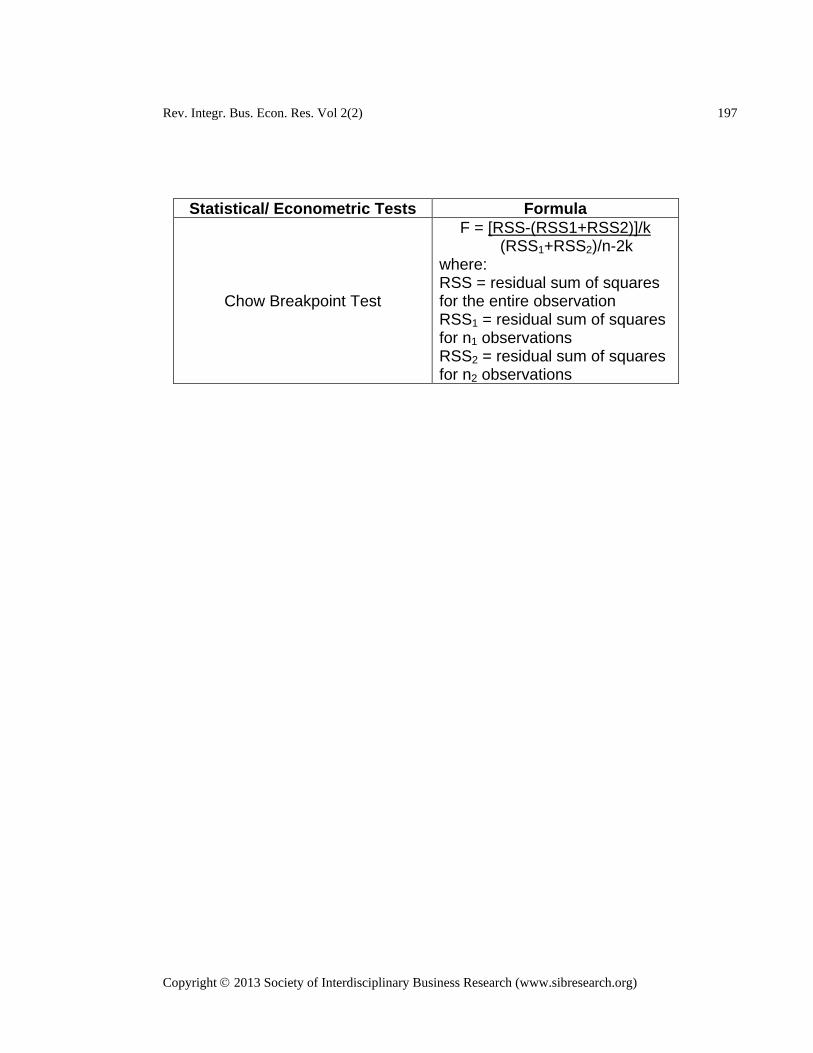
Rev. Integr. Bus. Econ. Res. Vol 2(2) 197
Copyright 2013 Society of Interdisciplinary Business Research (www.sibresearch.org)
Statistical/ Econometric Tests Formula
Chow Breakpoint Test
F = (RSS1+RSS2)/n-2k
[RSS-(RSS1+RSS2)]/k
where: RSS = residual sum of squares for the entire observation RSS1 = residual sum of squares for n1 observations RSS2 = residual sum of squares for n2 observations
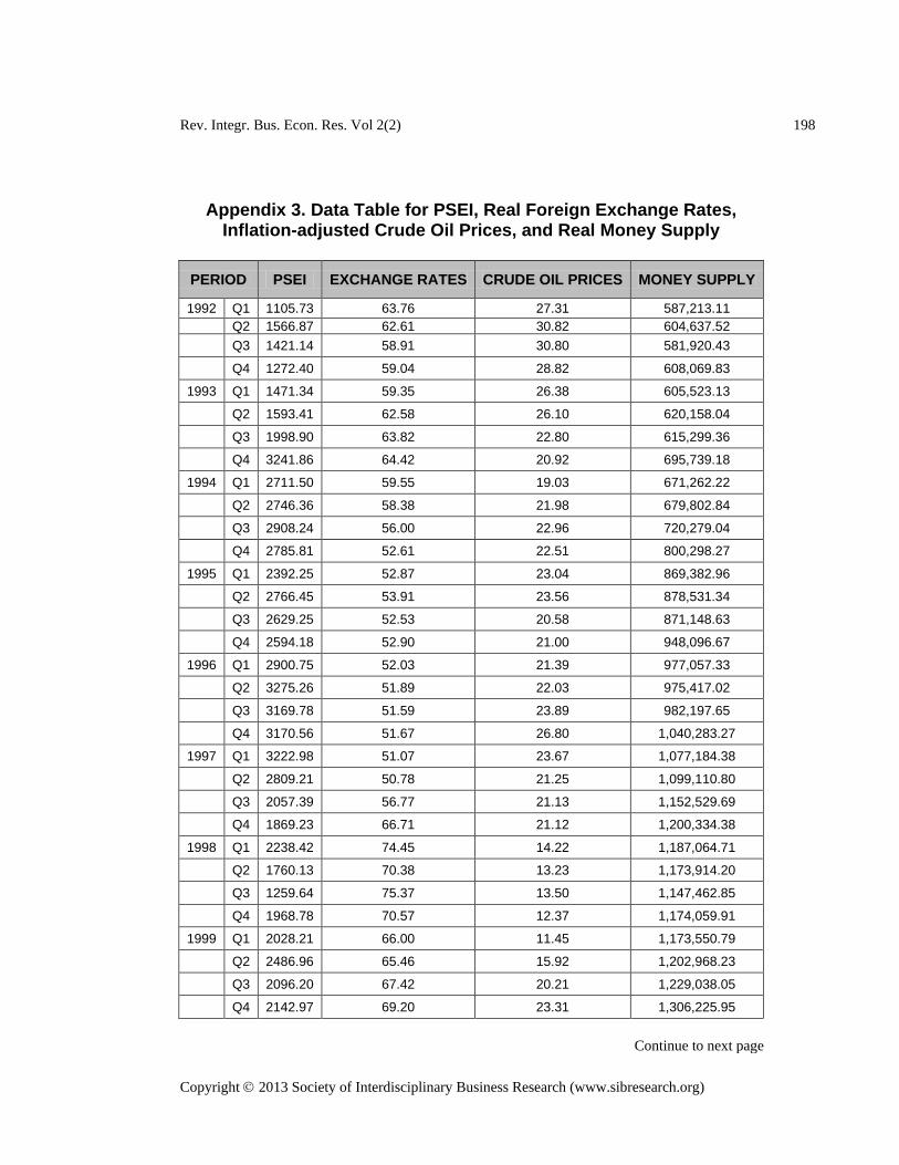
Rev. Integr. Bus. Econ. Res. Vol 2(2) 198
Copyright 2013 Society of Interdisciplinary Business Research (www.sibresearch.org)
Appendix 3. Data Table for PSEI, Real Foreign Exchange Rates, Inflation-adjusted Crude Oil Prices, and Real Money Supply
PERIOD PSEI EXCHANGE RATES CRUDE OIL PRICES MONEY SUPPLY
1992 Q1 1105.73 63.76 27.31 587,213.11 Q2 1566.87 62.61 30.82 604,637.52 Q3 1421.14 58.91 30.80 581,920.43
Q4 1272.40 59.04 28.82 608,069.83
1993 Q1 1471.34 59.35 26.38 605,523.13
Q2 1593.41 62.58 26.10 620,158.04
Q3 1998.90 63.82 22.80 615,299.36
Q4 3241.86 64.42 20.92 695,739.18
1994 Q1 2711.50 59.55 19.03 671,262.22
Q2 2746.36 58.38 21.98 679,802.84
Q3 2908.24 56.00 22.96 720,279.04
Q4 2785.81 52.61 22.51 800,298.27
1995 Q1 2392.25 52.87 23.04 869,382.96
Q2 2766.45 53.91 23.56 878,531.34
Q3 2629.25 52.53 20.58 871,148.63
Q4 2594.18 52.90 21.00 948,096.67
1996 Q1 2900.75 52.03 21.39 977,057.33
Q2 3275.26 51.89 22.03 975,417.02
Q3 3169.78 51.59 23.89 982,197.65
Q4 3170.56 51.67 26.80 1,040,283.27
1997 Q1 3222.98 51.07 23.67 1,077,184.38
Q2 2809.21 50.78 21.25 1,099,110.80
Q3 2057.39 56.77 21.13 1,152,529.69
Q4 1869.23 66.71 21.12 1,200,334.38
1998 Q1 2238.42 74.45 14.22 1,187,064.71
Q2 1760.13 70.38 13.23 1,173,914.20
Q3 1259.64 75.37 13.50 1,147,462.85
Q4 1968.78 70.57 12.37 1,174,059.91
1999 Q1 2028.21 66.00 11.45 1,173,550.79
Q2 2486.96 65.46 15.92 1,202,968.23
Q3 2096.20 67.42 20.21 1,229,038.05
Q4 2142.97 69.20 23.31 1,306,225.95
Continue to next page

Rev. Integr. Bus. Econ. Res. Vol 2(2) 199
Copyright 2013 Society of Interdisciplinary Business Research (www.sibresearch.org)
2000 Q1 1681.72 69.87 24.81 1,294,323.12
Q2 1533.99 72.13 25.26 1,306,170.10
Q3 1434.49 76.77 27.47 1,294,225.61
Q4 1494.50 82.56 26.74 1,333,830.15
2001 Q1 1446.40 81.40 22.45 1,358,535.32
Q2 1410.07 84.15 23.66 1,385,968.88
Q3 1126.63 85.31 22.22 1,346,440.66
Q4 1168.08 84.03 16.85 1,366,517.56
2002 Q1 1403.62 82.78 18.38 1,404,442.91
Q2 1156.35 81.84 22.16 1,425,238.59
Q3 1129.34 83.22 23.14 1,414,966.53
Q4 1018.41 86.04 22.61 1,460,941.69
2003 Q1 1039.67 87.28 25.47 1,449,998.22
Q2 1222.80 84.74 21.49 1,433,765.73
Q3 1297.42 86.96 23.15 1,414,342.94
Q4 1442.37 87.58 23.89 1,458,168.55
2004 Q1 1424.33 88.23 24.99 1,456,042.53
Q2 1579.40 87.90 27.77 1,452,027.50
Q3 1761.57 85.74 29.49 1,403,958.59
Q4 1822.83 85.27 28.58 1,449,772.36
2005 Q1 1954.69 82.39 32.43 1,503,288.76
Q2 1924.23 81.84 37.13 1,509,117.54
Q3 1942.07 83.28 42.22 1,507,898.27
Q4 2096.04 80.33 39.59 1,507,836.25
2006 Q1 2195.95 75.10 42.57 1,503,633.55
Q2 2178.79 76.10 47.10 1,563,371.84
Q3 2556.71 74.36 47.36 1,595,679.29
Q4 2982.54 71.14 41.11 1,711,152.96
2007 Q1 3203.55 69.98 39.75 2,039,392.85
Q2 3660.86 68.59 46.04 2,123,779.94
Q3 3572.90 66.34 49.07 2,032,254.56
Q4 3621.60 62.10 57.76 2,076,793.15
2008 Q1 2984.67 58.26 61.87 2,038,095.10
Q2 2459.98 59.88 75.63 1,990,311.37
Q3 2569.65 61.84 70.93 1,974,224.21
Q4 1872.85 64.56 33.97 2,167,652.95
Continue to next page
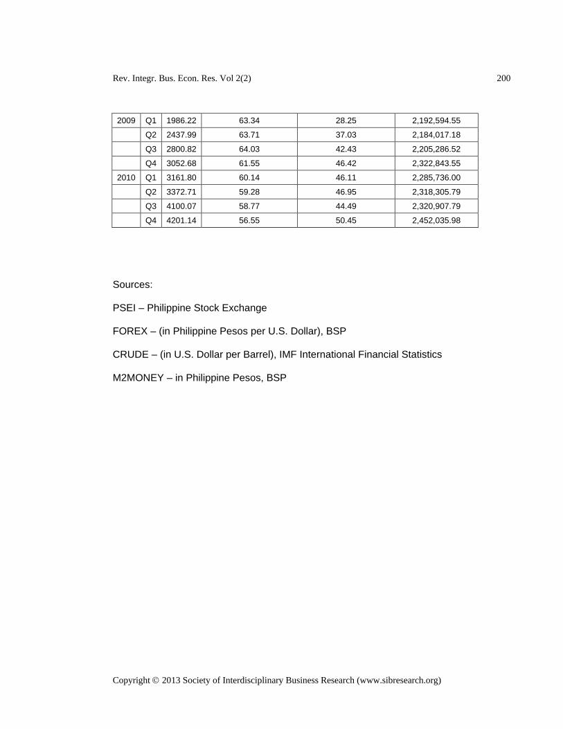
Rev. Integr. Bus. Econ. Res. Vol 2(2) 200
Copyright 2013 Society of Interdisciplinary Business Research (www.sibresearch.org)
2009 Q1 1986.22 63.34 28.25 2,192,594.55
Q2 2437.99 63.71 37.03 2,184,017.18
Q3 2800.82 64.03 42.43 2,205,286.52
Q4 3052.68 61.55 46.42 2,322,843.55
2010 Q1 3161.80 60.14 46.11 2,285,736.00
Q2 3372.71 59.28 46.95 2,318,305.79
Q3 4100.07 58.77 44.49 2,320,907.79
Q4 4201.14 56.55 50.45 2,452,035.98
Sources:
PSEI – Philippine Stock Exchange
FOREX – (in Philippine Pesos per U.S. Dollar), BSP
CRUDE – (in U.S. Dollar per Barrel), IMF International Financial Statistics
M2MONEY – in Philippine Pesos, BSP
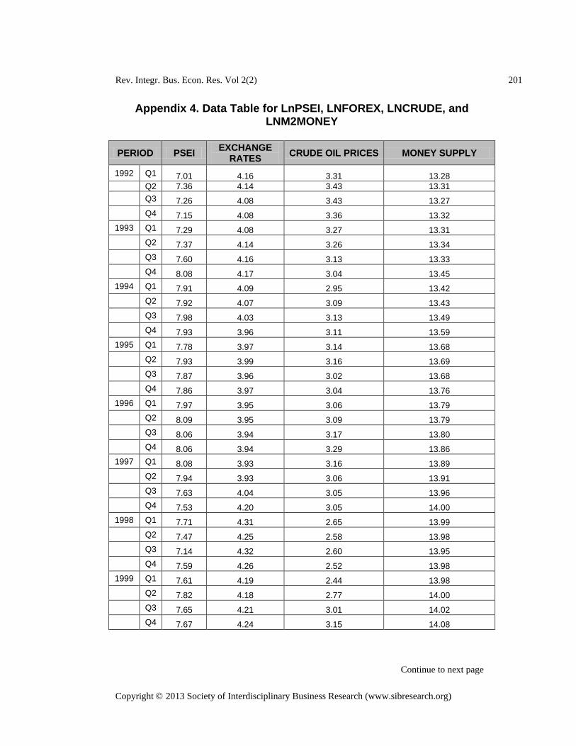
Rev. Integr. Bus. Econ. Res. Vol 2(2) 201
Copyright 2013 Society of Interdisciplinary Business Research (www.sibresearch.org)
Appendix 4. Data Table for LnPSEI, LNFOREX, LNCRUDE, and LNM2MONEY
PERIOD PSEI EXCHANGE
RATES CRUDE OIL PRICES MONEY SUPPLY
1992 Q1 7.01 4.16 3.31 13.28 Q2 7.36 4.14 3.43 13.31 Q3 7.26 4.08 3.43 13.27 Q4 7.15 4.08 3.36 13.32
1993 Q1 7.29 4.08 3.27 13.31 Q2 7.37 4.14 3.26 13.34 Q3 7.60 4.16 3.13 13.33 Q4 8.08 4.17 3.04 13.45
1994 Q1 7.91 4.09 2.95 13.42 Q2 7.92 4.07 3.09 13.43 Q3 7.98 4.03 3.13 13.49 Q4 7.93 3.96 3.11 13.59
1995 Q1 7.78 3.97 3.14 13.68 Q2 7.93 3.99 3.16 13.69 Q3 7.87 3.96 3.02 13.68 Q4 7.86 3.97 3.04 13.76
1996 Q1 7.97 3.95 3.06 13.79 Q2 8.09 3.95 3.09 13.79 Q3 8.06 3.94 3.17 13.80 Q4 8.06 3.94 3.29 13.86
1997 Q1 8.08 3.93 3.16 13.89 Q2 7.94 3.93 3.06 13.91 Q3 7.63 4.04 3.05 13.96 Q4 7.53 4.20 3.05 14.00
1998 Q1 7.71 4.31 2.65 13.99 Q2 7.47 4.25 2.58 13.98 Q3 7.14 4.32 2.60 13.95 Q4 7.59 4.26 2.52 13.98
1999 Q1 7.61 4.19 2.44 13.98 Q2 7.82 4.18 2.77 14.00 Q3 7.65 4.21 3.01 14.02 Q4 7.67 4.24 3.15 14.08
Continue to next page
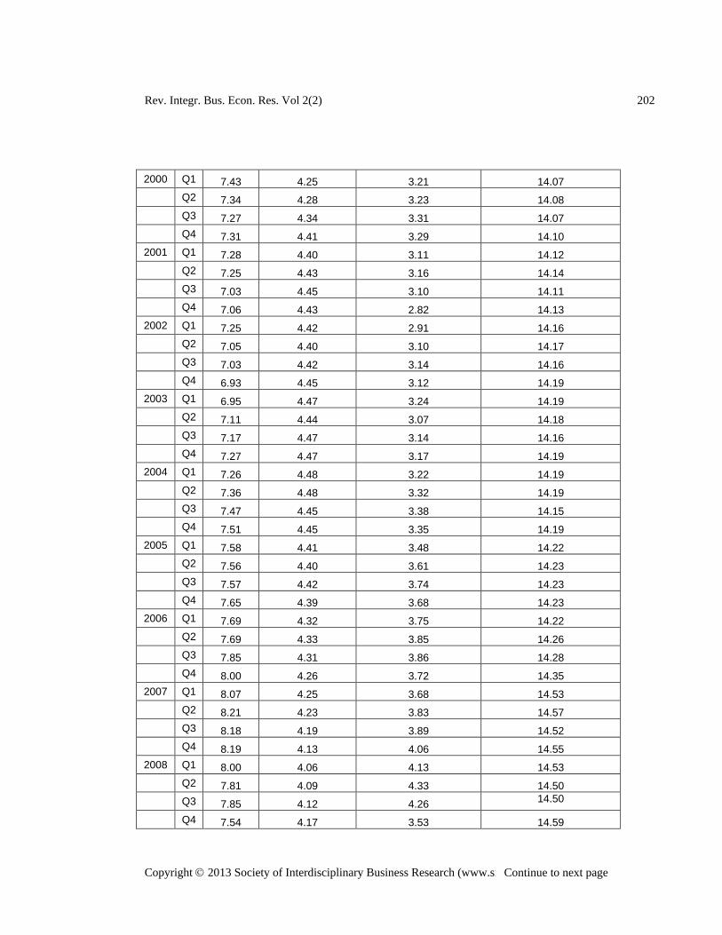
Rev. Integr. Bus. Econ. Res. Vol 2(2) 202
Copyright 2013 Society of Interdisciplinary Business Research (www.sibresearch.org)
2000 Q1 7.43 4.25 3.21 14.07 Q2 7.34 4.28 3.23 14.08 Q3 7.27 4.34 3.31 14.07 Q4 7.31 4.41 3.29 14.10
2001 Q1 7.28 4.40 3.11 14.12 Q2 7.25 4.43 3.16 14.14 Q3 7.03 4.45 3.10 14.11 Q4 7.06 4.43 2.82 14.13
2002 Q1 7.25 4.42 2.91 14.16 Q2 7.05 4.40 3.10 14.17 Q3 7.03 4.42 3.14 14.16 Q4 6.93 4.45 3.12 14.19
2003 Q1 6.95 4.47 3.24 14.19 Q2 7.11 4.44 3.07 14.18 Q3 7.17 4.47 3.14 14.16 Q4 7.27 4.47 3.17 14.19
2004 Q1 7.26 4.48 3.22 14.19 Q2 7.36 4.48 3.32 14.19 Q3 7.47 4.45 3.38 14.15 Q4 7.51 4.45 3.35 14.19
2005 Q1 7.58 4.41 3.48 14.22 Q2 7.56 4.40 3.61 14.23 Q3 7.57 4.42 3.74 14.23 Q4 7.65 4.39 3.68 14.23
2006 Q1 7.69 4.32 3.75 14.22 Q2 7.69 4.33 3.85 14.26 Q3 7.85 4.31 3.86 14.28 Q4 8.00 4.26 3.72 14.35
2007 Q1 8.07 4.25 3.68 14.53 Q2 8.21 4.23 3.83 14.57 Q3 8.18 4.19 3.89 14.52 Q4 8.19 4.13 4.06 14.55
2008 Q1 8.00 4.06 4.13 14.53 Q2 7.81 4.09 4.33 14.50 Q3 7.85 4.12 4.26 14.50
Q4 7.54 4.17 3.53 14.59
Continue to next page

Rev. Integr. Bus. Econ. Res. Vol 2(2) 203
Copyright 2013 Society of Interdisciplinary Business Research (www.sibresearch.org)
2009 Q1 7.59 4.15 3.34 14.60 Q2 7.80 4.15 3.61 14.60 Q3 7.94 4.16 3.75 14.61 Q4 8.02 4.12 3.84 14.66
2010 Q1 8.06 4.10 3.83 14.64 Q2 8.12 4.08 3.85 14.66 Q3 8.32 4.07 3.80 14.66 Q4 8.34 4.04 3.92 14.71
*Values are computed by the author
*Exchange rates in Peso per US Dollar, Crude oil prices in US$ per barrel
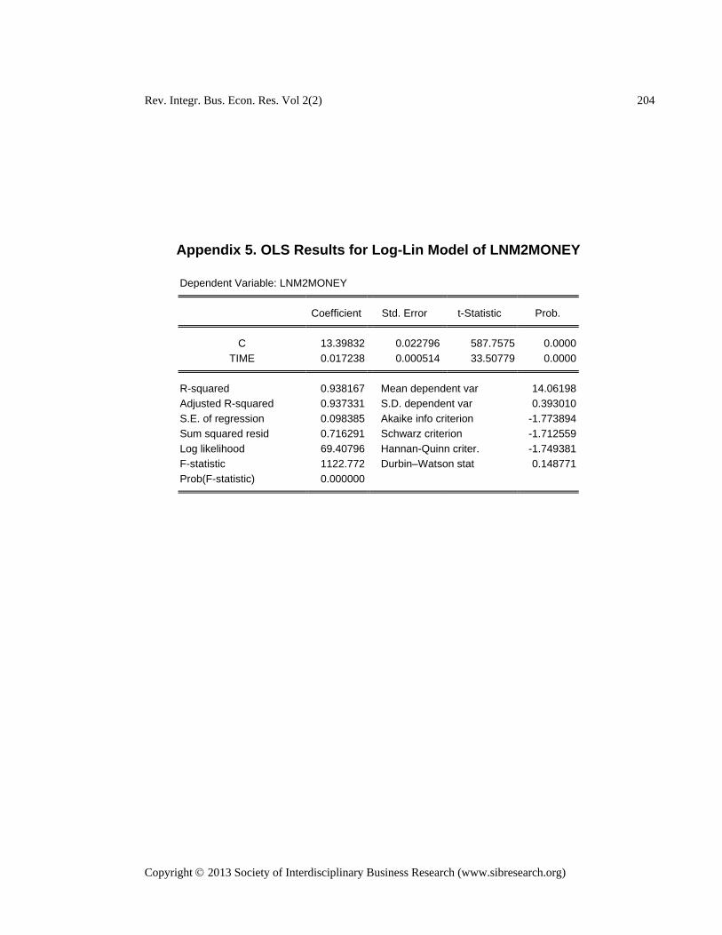
Rev. Integr. Bus. Econ. Res. Vol 2(2) 204
Copyright 2013 Society of Interdisciplinary Business Research (www.sibresearch.org)
Appendix 5. OLS Results for Log-Lin Model of LNM2MONEY
Dependent Variable: LNM2MONEY Coefficient Std. Error t-Statistic Prob. C 13.39832 0.022796 587.7575 0.0000
TIME 0.017238 0.000514 33.50779 0.0000 R-squared 0.938167 Mean dependent var 14.06198
Adjusted R-squared 0.937331 S.D. dependent var 0.393010 S.E. of regression 0.098385 Akaike info criterion -1.773894 Sum squared resid 0.716291 Schwarz criterion -1.712559 Log likelihood 69.40796 Hannan-Quinn criter. -1.749381 F-statistic 1122.772 Durbin–Watson stat 0.148771 Prob(F-statistic) 0.000000

Rev. Integr. Bus. Econ. Res. Vol 2(2) 205
Copyright 2013 Society of Interdisciplinary Business Research (www.sibresearch.org)
Appendix 6. Augmented Dickey–Fuller Test Results on LNPSEI
t-Statistic Prob.*
Augmented Dickey–Fuller test statistic -1.445372 0.5555 Test critical values: 1% level -3.521579
5% level -2.901217 10% level -2.587981 *MacKinnon (1996) one-sided p-values.
Included observations: 74 after adjustments Coefficient Std. Error t-Statistic Prob. LNPSEI(-1) -0.073265 0.050689 -1.445372 0.1528
D(LNPSEI(-1)) 0.060289 0.116395 0.517973 0.6061 C 0.571580 0.386907 1.477305 0.1440 R-squared 0.029067 Mean dependent var 0.013328
Adjusted R-squared 0.001717 S.D. dependent var 0.152019 S.E. of regression 0.151888 Akaike info criterion -0.891648 Sum squared resid 1.637973 Schwarz criterion -0.798240 Log likelihood 35.99096 Hannan-Quinn criter. -0.854386 F-statistic 1.062766 Durbin–Watson stat 1.930931 Prob(F-statistic) 0.350930
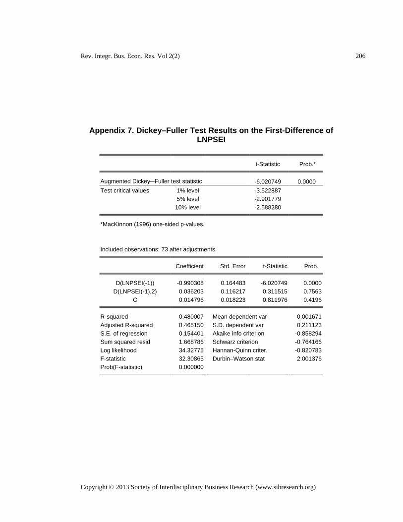
Rev. Integr. Bus. Econ. Res. Vol 2(2) 206
Copyright 2013 Society of Interdisciplinary Business Research (www.sibresearch.org)
Appendix 7. Dickey–Fuller Test Results on the First-Difference of LNPSEI
t-Statistic Prob.*
Augmented Dickey–Fuller test statistic -6.020749 0.0000 Test critical values: 1% level -3.522887
5% level -2.901779 10% level -2.588280 *MacKinnon (1996) one-sided p-values.
Included observations: 73 after adjustments Coefficient Std. Error t-Statistic Prob. D(LNPSEI(-1)) -0.990308 0.164483 -6.020749 0.0000
D(LNPSEI(-1),2) 0.036203 0.116217 0.311515 0.7563 C 0.014796 0.018223 0.811976 0.4196 R-squared 0.480007 Mean dependent var 0.001671
Adjusted R-squared 0.465150 S.D. dependent var 0.211123 S.E. of regression 0.154401 Akaike info criterion -0.858294 Sum squared resid 1.668786 Schwarz criterion -0.764166 Log likelihood 34.32775 Hannan-Quinn criter. -0.820783 F-statistic 32.30865 Durbin–Watson stat 2.001376 Prob(F-statistic) 0.000000

Rev. Integr. Bus. Econ. Res. Vol 2(2) 207
Copyright 2013 Society of Interdisciplinary Business Research (www.sibresearch.org)
Appendix 8. Dickey–Fuller Test Results on LNFOREX
t-Statistic Prob.*
Augmented Dickey–Fuller test statistic -1.400336 0.5777 Test critical values: 1% level -3.521579
5% level -2.901217 10% level -2.587981 *MacKinnon (1996) one-sided p-values.
Included observations: 74 after adjustments Coefficient Std. Error t-Statistic Prob. LNFOREX(-1) -0.038163 0.027253 -1.400336 0.1658
D(LNFOREX(-1)) 0.392191 0.110325 3.554879 0.0007 C 0.159974 0.115024 1.390790 0.1686 R-squared 0.159505 Mean dependent var -0.001376
Adjusted R-squared 0.135829 S.D. dependent var 0.042835 S.E. of regression 0.039819 Akaike info criterion -3.569227 Sum squared resid 0.112577 Schwarz criterion -3.475819 Log likelihood 135.0614 Hannan-Quinn criter. -3.531966 F-statistic 6.736999 Durbin–Watson stat 1.979032 Prob(F-statistic) 0.002094

Rev. Integr. Bus. Econ. Res. Vol 2(2) 208
Copyright 2013 Society of Interdisciplinary Business Research (www.sibresearch.org)
Appendix 9. Dickey–Fuller Test Results on the First-Difference of LNFOREX
t-Statistic Prob.*
Augmented Dickey–Fuller test statistic -4.903876 0.0001 Test critical values: 1% level -3.522887
5% level -2.901779 10% level -2.588280 *MacKinnon (1996) one-sided p-values.
Included observations: 73 after adjustments Coefficient Std. Error t-Statistic Prob. D(LNFOREX(-1)) -0.653038 0.133168 -4.903876 0.0000
D(LNFOREX(-1),2) 0.026616 0.118493 0.224617 0.8229 C -0.000263 0.004699 -0.055919 0.9556 R-squared 0.322811 Mean dependent var 0.000307
Adjusted R-squared 0.303463 S.D. dependent var 0.048084 S.E. of regression 0.040130 Akaike info criterion -3.553156 Sum squared resid 0.112729 Schwarz criterion -3.459028 Log likelihood 132.6902 Hannan-Quinn criter. -3.515644 F-statistic 16.68428 Durbin–Watson stat 1.960667 Prob(F-statistic) 0.000001
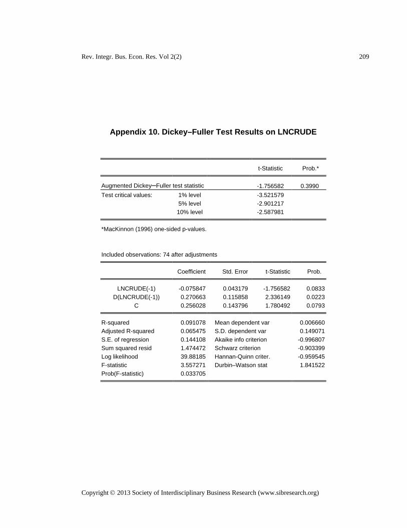
Rev. Integr. Bus. Econ. Res. Vol 2(2) 209
Copyright 2013 Society of Interdisciplinary Business Research (www.sibresearch.org)
Appendix 10. Dickey–Fuller Test Results on LNCRUDE
t-Statistic Prob.*
Augmented Dickey–Fuller test statistic -1.756582 0.3990 Test critical values: 1% level -3.521579
5% level -2.901217 10% level -2.587981 *MacKinnon (1996) one-sided p-values.
Included observations: 74 after adjustments Coefficient Std. Error t-Statistic Prob. LNCRUDE(-1) -0.075847 0.043179 -1.756582 0.0833
D(LNCRUDE(-1)) 0.270663 0.115858 2.336149 0.0223 C 0.256028 0.143796 1.780492 0.0793 R-squared 0.091078 Mean dependent var 0.006660
Adjusted R-squared 0.065475 S.D. dependent var 0.149071 S.E. of regression 0.144108 Akaike info criterion -0.996807 Sum squared resid 1.474472 Schwarz criterion -0.903399 Log likelihood 39.88185 Hannan-Quinn criter. -0.959545 F-statistic 3.557271 Durbin–Watson stat 1.841522 Prob(F-statistic) 0.033705
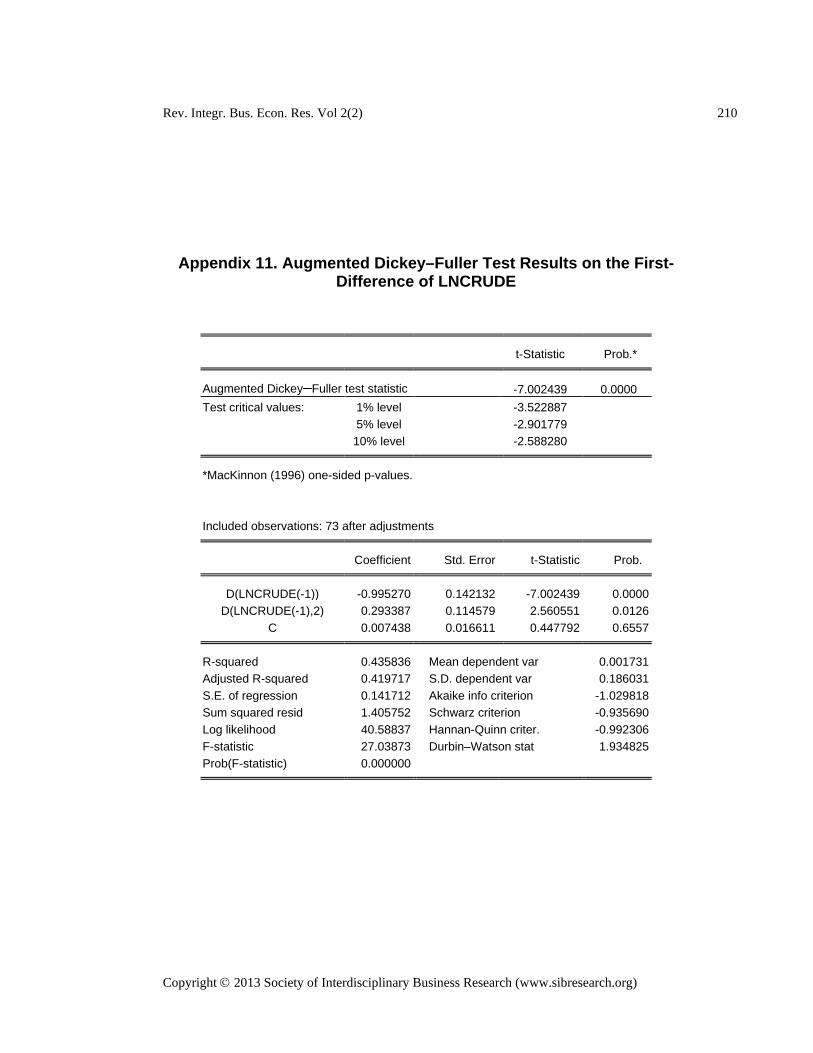
Rev. Integr. Bus. Econ. Res. Vol 2(2) 210
Copyright 2013 Society of Interdisciplinary Business Research (www.sibresearch.org)
Appendix 11. Augmented Dickey–Fuller Test Results on the First-Difference of LNCRUDE
t-Statistic Prob.*
Augmented Dickey–Fuller test statistic -7.002439 0.0000 Test critical values: 1% level -3.522887
5% level -2.901779 10% level -2.588280 *MacKinnon (1996) one-sided p-values.
Included observations: 73 after adjustments Coefficient Std. Error t-Statistic Prob. D(LNCRUDE(-1)) -0.995270 0.142132 -7.002439 0.0000
D(LNCRUDE(-1),2) 0.293387 0.114579 2.560551 0.0126 C 0.007438 0.016611 0.447792 0.6557 R-squared 0.435836 Mean dependent var 0.001731
Adjusted R-squared 0.419717 S.D. dependent var 0.186031 S.E. of regression 0.141712 Akaike info criterion -1.029818 Sum squared resid 1.405752 Schwarz criterion -0.935690 Log likelihood 40.58837 Hannan-Quinn criter. -0.992306 F-statistic 27.03873 Durbin–Watson stat 1.934825 Prob(F-statistic) 0.000000
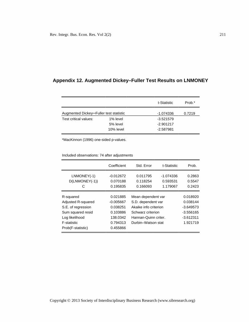
Rev. Integr. Bus. Econ. Res. Vol 2(2) 211
Copyright 2013 Society of Interdisciplinary Business Research (www.sibresearch.org)
Appendix 12. Augmented Dickey–Fuller Test Results on LNMONEY
t-Statistic Prob.*
Augmented Dickey–Fuller test statistic -1.074336 0.7219 Test critical values: 1% level -3.521579
5% level -2.901217 10% level -2.587981 *MacKinnon (1996) one-sided p-values.
Included observations: 74 after adjustments Coefficient Std. Error t-Statistic Prob. LNMONEY(-1) -0.012672 0.011795 -1.074336 0.2863
D(LNMONEY(-1)) 0.070188 0.118254 0.593531 0.5547 C 0.195835 0.166093 1.179067 0.2423 R-squared 0.021885 Mean dependent var 0.018920
Adjusted R-squared -0.005667 S.D. dependent var 0.038144 S.E. of regression 0.038251 Akaike info criterion -3.649573 Sum squared resid 0.103886 Schwarz criterion -3.556165 Log likelihood 138.0342 Hannan-Quinn criter. -3.612311 F-statistic 0.794313 Durbin–Watson stat 1.921719 Prob(F-statistic) 0.455866

Rev. Integr. Bus. Econ. Res. Vol 2(2) 212
Copyright 2013 Society of Interdisciplinary Business Research (www.sibresearch.org)
Appendix 13. Augmented Dickey–Fuller Test Results on the First-Difference of LNMONEY
t-Statistic Prob.*
Augmented Dickey–Fuller test statistic -6.317897 0.0000 Test critical values: 1% level -3.522887
5% level -2.901779 10% level -2.588280 *MacKinnon (1996) one-sided p-values.
Included observations: 73 after adjustments Coefficient Std. Error t-Statistic Prob. D(LNMONEY(-1)) -1.007544 0.159475 -6.317897 0.0000
D(LNMONEY(-1),2) 0.099703 0.117880 0.845806 0.4005 C 0.019881 0.005348 3.717076 0.0004 R-squared 0.468360 Mean dependent var 0.001277
Adjusted R-squared 0.453171 S.D. dependent var 0.051398 S.E. of regression 0.038008 Akaike info criterion -3.661821 Sum squared resid 0.101122 Schwarz criterion -3.567692 Log likelihood 136.6565 Hannan-Quinn criter. -3.624309 F-statistic 30.83406 Durbin–Watson stat 1.955725 Prob(F-statistic) 0.000000
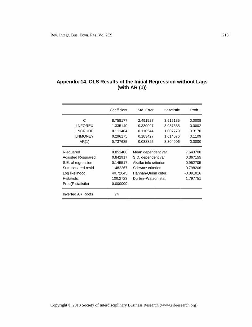
Rev. Integr. Bus. Econ. Res. Vol 2(2) 213
Copyright 2013 Society of Interdisciplinary Business Research (www.sibresearch.org)
Appendix 14. OLS Results of the Initial Regression without Lags (with AR (1))
Coefficient Std. Error t-Statistic Prob. C 8.758177 2.491527 3.515185 0.0008
LNFOREX -1.335140 0.339097 -3.937335 0.0002 LNCRUDE 0.111404 0.110544 1.007779 0.3170 LNMONEY 0.296175 0.183427 1.614676 0.1109
AR(1) 0.737685 0.088825 8.304906 0.0000 R-squared 0.851408 Mean dependent var 7.643700
Adjusted R-squared 0.842917 S.D. dependent var 0.367155 S.E. of regression 0.145517 Akaike info criterion -0.952705 Sum squared resid 1.482267 Schwarz criterion -0.798206 Log likelihood 40.72645 Hannan-Quinn criter. -0.891016 F-statistic 100.2723 Durbin–Watson stat 1.797751 Prob(F-statistic) 0.000000
Inverted AR Roots .74
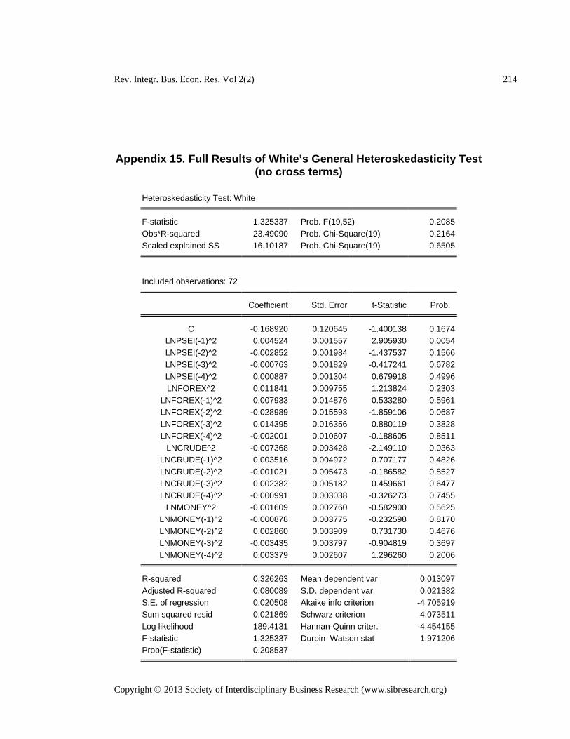
Rev. Integr. Bus. Econ. Res. Vol 2(2) 214
Copyright 2013 Society of Interdisciplinary Business Research (www.sibresearch.org)
Appendix 15. Full Results of White’s General Heteroskedasticity Test (no cross terms)
Heteroskedasticity Test: White
F-statistic 1.325337 Prob. F(19,52) 0.2085
Obs*R-squared 23.49090 Prob. Chi-Square(19) 0.2164 Scaled explained SS 16.10187 Prob. Chi-Square(19) 0.6505
Included observations: 72 Coefficient Std. Error t-Statistic Prob. C -0.168920 0.120645 -1.400138 0.1674
LNPSEI(-1)^2 0.004524 0.001557 2.905930 0.0054 LNPSEI(-2)^2 -0.002852 0.001984 -1.437537 0.1566 LNPSEI(-3)^2 -0.000763 0.001829 -0.417241 0.6782 LNPSEI(-4)^2 0.000887 0.001304 0.679918 0.4996 LNFOREX^2 0.011841 0.009755 1.213824 0.2303
LNFOREX(-1)^2 0.007933 0.014876 0.533280 0.5961 LNFOREX(-2)^2 -0.028989 0.015593 -1.859106 0.0687 LNFOREX(-3)^2 0.014395 0.016356 0.880119 0.3828 LNFOREX(-4)^2 -0.002001 0.010607 -0.188605 0.8511
LNCRUDE^2 -0.007368 0.003428 -2.149110 0.0363 LNCRUDE(-1)^2 0.003516 0.004972 0.707177 0.4826 LNCRUDE(-2)^2 -0.001021 0.005473 -0.186582 0.8527 LNCRUDE(-3)^2 0.002382 0.005182 0.459661 0.6477 LNCRUDE(-4)^2 -0.000991 0.003038 -0.326273 0.7455
LNMONEY^2 -0.001609 0.002760 -0.582900 0.5625 LNMONEY(-1)^2 -0.000878 0.003775 -0.232598 0.8170 LNMONEY(-2)^2 0.002860 0.003909 0.731730 0.4676 LNMONEY(-3)^2 -0.003435 0.003797 -0.904819 0.3697 LNMONEY(-4)^2 0.003379 0.002607 1.296260 0.2006
R-squared 0.326263 Mean dependent var 0.013097
Adjusted R-squared 0.080089 S.D. dependent var 0.021382 S.E. of regression 0.020508 Akaike info criterion -4.705919 Sum squared resid 0.021869 Schwarz criterion -4.073511 Log likelihood 189.4131 Hannan-Quinn criter. -4.454155 F-statistic 1.325337 Durbin–Watson stat 1.971206 Prob(F-statistic) 0.208537

Rev. Integr. Bus. Econ. Res. Vol 2(2) 215
Copyright 2013 Society of Interdisciplinary Business Research (www.sibresearch.org)
Appendix 16. Full Results of Autoregressive Conditional Heteroskedasticity Test
Heteroskedasticity Test: ARCH F-statistic 1.206177 Prob. F(1,69) 0.2759
Obs*R-squared 1.219815 Prob. Chi-Square(1) 0.2694
Test Equation: Dependent Variable: RESID^2 Method: Least Squares Date: 11/21/11 Time: 17:10 Sample (adjusted): 1993Q2 2010Q4 Included observations: 71 after adjustments
Coefficient Std. Error t-Statistic Prob. C 0.011523 0.002994 3.848560 0.0003
RESID^2(-1) 0.130942 0.119226 1.098261 0.2759 R-squared 0.017180 Mean dependent var 0.013252
Adjusted R-squared 0.002937 S.D. dependent var 0.021493 S.E. of regression 0.021461 Akaike info criterion -4.817362 Sum squared resid 0.031781 Schwarz criterion -4.753625 Log likelihood 173.0164 Hannan-Quinn criter. -4.792016 F-statistic 1.206177 Durbin–Watson stat 1.997476 Prob(F-statistic) 0.275908

Rev. Integr. Bus. Econ. Res. Vol 2(2) 216
Copyright 2013 Society of Interdisciplinary Business Research (www.sibresearch.org)
Appendix 17. Full Results of Breusch–Godfrey/Lagrange Multiplier Test
Breusch–Godfrey Serial Correlation LM Test:
F-statistic 0.141602 Prob. F(4,48) 0.9658 Obs*R-squared 0.839702 Prob. Chi-Square(4) 0.9330
Coefficient Std. Error t-Statistic Prob. C -0.521104 2.264752 -0.230093 0.8190
LNPSEI(-1) 0.263933 0.451531 0.584530 0.5616 LNPSEI(-2) -0.282438 0.585361 -0.482502 0.6316 LNPSEI(-3) 0.066910 0.385107 0.173745 0.8628 LNPSEI(-4) 0.000545 0.189474 0.002876 0.9977 LNFOREX -0.053192 0.605174 -0.087895 0.9303
LNFOREX(-1) 0.550108 1.311516 0.419444 0.6768 LNFOREX(-2) -0.982089 1.889049 -0.519886 0.6055 LNFOREX(-3) 0.859925 1.864568 0.461193 0.6467 LNFOREX(-4) -0.334579 0.943734 -0.354526 0.7245
LNCRUDE -0.003765 0.168128 -0.022391 0.9822 LNCRUDE(-1) -0.048618 0.251116 -0.193607 0.8473 LNCRUDE(-2) 0.054964 0.275748 0.199327 0.8428 LNCRUDE(-3) 0.031141 0.251492 0.123827 0.9020 LNCRUDE(-4) -0.051811 0.158497 -0.326890 0.7452
LNMONEY 0.040333 0.569468 0.070826 0.9438 LNMONEY(-1) -0.353669 0.957143 -0.369505 0.7134 LNMONEY(-2) 0.497386 1.148914 0.432919 0.6670 LNMONEY(-3) -0.366298 1.088714 -0.336450 0.7380 LNMONEY(-4) 0.185124 0.645803 0.286656 0.7756
RESID(-1) -0.306042 0.473319 -0.646587 0.5210 RESID(-2) 0.085061 0.373318 0.227850 0.8207 RESID(-3) -0.004493 0.302597 -0.014849 0.9882 RESID(-4) 0.035814 0.211096 0.169656 0.8660
R-squared 0.011663 Mean dependent var -3.20E-15
Adjusted R-squared -0.461916 S.D. dependent var 0.115245 S.E. of regression 0.139342 Akaike info criterion -0.842563 Sum squared resid 0.931983 Schwarz criterion -0.083674 Log likelihood 54.33226 Hannan-Quinn criter. -0.540447 F-statistic 0.024626 Durbin–Watson stat 2.008580 Prob(F-statistic) 1.000000

Rev. Integr. Bus. Econ. Res. Vol 2(2) 217
Copyright 2013 Society of Interdisciplinary Business Research (www.sibresearch.org)
Appendix 18. Full Results of Ramsey’s RESET
Ramsey RESET Test: F-statistic 0.733045 Prob. F(1,51) 0.3959
Log likelihood ratio 1.027521 Prob. Chi-Square(1) 0.3107
Included observations: 72 Coefficient Std. Error t-Statistic Prob. C 4.148757 1.563585 2.653362 0.0106
LNPSEI(-1) 2.400368 1.889234 1.270551 0.2097 LNPSEI(-2) -0.162997 0.235529 -0.692045 0.4920 LNPSEI(-3) 0.274065 0.280230 0.978000 0.3327 LNPSEI(-4) -0.572600 0.475066 -1.205306 0.2336 LNFOREX -5.109179 4.085566 -1.250544 0.2168
LNFOREX(-1) 7.935018 6.291527 1.261223 0.2130 LNFOREX(-2) -5.475324 4.353153 -1.257784 0.2142 LNFOREX(-3) 1.063708 1.251706 0.849807 0.3994 LNFOREX(-4) 0.182604 0.628379 0.290594 0.7725
LNCRUDE 0.723998 0.591756 1.223474 0.2268 LNCRUDE(-1) -0.797388 0.664681 -1.199655 0.2358 LNCRUDE(-2) 0.189613 0.287357 0.659853 0.5123 LNCRUDE(-3) -0.396989 0.395262 -1.004368 0.3199 LNCRUDE(-4) 0.665142 0.541218 1.228972 0.2247
LNMONEY 3.312743 2.670661 1.240421 0.2205 LNMONEY(-1) -4.457052 3.575377 -1.246597 0.2182 LNMONEY(-2) 3.114589 2.568164 1.212769 0.2308 LNMONEY(-3) -2.869603 2.344632 -1.223903 0.2266 LNMONEY(-4) 0.985788 0.877549 1.123343 0.2666
FITTED^2 -0.135268 0.157990 -0.856181 0.3959 R-squared 0.901953 Mean dependent var 7.659900
Adjusted R-squared 0.863503 S.D. dependent var 0.365431 S.E. of regression 0.135010 Akaike info criterion -0.928436 Sum squared resid 0.929619 Schwarz criterion -0.264408 Log likelihood 54.42370 Hannan-Quinn criter. -0.664085 F-statistic 23.45787 Durbin–Watson stat 2.077292 Prob(F-statistic) 0.000000

Rev. Integr. Bus. Econ. Res. Vol 2(2) 218
Copyright 2013 Society of Interdisciplinary Business Research (www.sibresearch.org)
Appendix 19. Full Results of Johansen Cointegration Test
Option 2 - Intercept (no trend) in CE – no intercept in VAR
Trend assumption: No deterministic trend (restricted constant)
Unrestricted Cointegration Rank Test (Trace) Hypothesized Trace 0.05
No. of CE(s) Eigenvalue Statistic Critical Value Prob.** None * 0.291418 65.96315 54.07904 0.0031
At most 1 * 0.230365 41.50442 35.19275 0.0091 At most 2 * 0.201120 22.91383 20.26184 0.0211 At most 3 0.093520 6.971208 9.164546 0.1279
Trace test indicates 3 cointegrating eqn(s) at the 0.05 level * denotes rejection of the hypothesis at the 0.05 level **MacKinnon-Haug-Michelis (1999) p-values
Unrestricted Cointegration Rank Test (Maximum Eigenvalue) Hypothesized Max-Eigen 0.05
No. of CE(s) Eigenvalue Statistic Critical Value Prob.** None 0.291418 24.45873 28.58808 0.1543
At most 1 0.230365 18.59059 22.29962 0.1523 At most 2 * 0.201120 15.94262 15.89210 0.0491 At most 3 0.093520 6.971208 9.164546 0.1279
Max-eigenvalue test indicates no cointegration at the 0.05 level * denotes rejection of the hypothesis at the 0.05 level **MacKinnon-Haug-Michelis (1999) p-values
Unrestricted Cointegrating Coefficients (normalized by b'*S11*b=I): LNPSEI LNRFOREX LNCRUDE LNM2MONEY C
5.264090 9.932630 -3.872665 1.242245 -86.77364 1.471863 2.068999 -0.964934 -1.129219 0.610022 6.650462 10.89815 1.819515 -3.903152 -47.35028 1.545006 -4.196608 -1.871182 0.568407 4.165269
Continue to next page

Rev. Integr. Bus. Econ. Res. Vol 2(2) 219
Copyright 2013 Society of Interdisciplinary Business Research (www.sibresearch.org)
Unrestricted Adjustment Coefficients (alpha): D(LNPSEI) -0.018094 0.018226 -0.014749 -0.036859 D(LNRFOREX) -0.006648 0.005482 -0.008143 0.006127 D(LNCRUDE) 0.043565 0.002187 -0.035246 -0.002808
D(LNM2MONEY) -0.001171 0.016256 0.003894 0.000680 1 Cointegrating Equation(s): Log likelihood 398.3929 Normalized cointegrating coefficients (standard error in parentheses)
LNPSEI LNRFOREX LNCRUDE LNM2MONEY C 1.000000 1.886865 -0.735676 0.235985 -16.48407
(0.31539) (0.18326) (0.18587) (2.10233)
Adjustment coefficients (standard error in parentheses) D(LNPSEI) -0.095251
(0.09570) D(LNRFOREX) -0.034994
(0.02230) D(LNCRUDE) 0.229331
(0.07478) D(LNM2MONEY) -0.006162
(0.02513) 2 Cointegrating Equation(s): Log likelihood 407.6882 Normalized cointegrating coefficients (standard error in parentheses)
LNPSEI LNRFOREX LNCRUDE LNM2MONEY C 1.000000 0.000000 -0.421610 -3.697971 49.78268
(2.99884) (2.86997) (34.2087) 0.000000 1.000000 -0.166448 2.084916 -35.12002
(1.60871) (1.53958) (18.3511)
Adjustment coefficients (standard error in parentheses) D(LNPSEI) -0.068425 -0.142017
(0.09844) (0.18272) D(LNRFOREX) -0.026924 -0.054685
(0.02279) (0.04231) D(LNCRUDE) 0.232550 0.437241
(0.07763) (0.14409) D(LNM2MONEY) 0.017765 0.022007
(0.02313) (0.04292)
Continue to next page

Rev. Integr. Bus. Econ. Res. Vol 2(2) 220
Copyright 2013 Society of Interdisciplinary Business Research (www.sibresearch.org)
3 Cointegrating Equation(s): Log likelihood 415.6595 Normalized cointegrating coefficients (standard error in parentheses)
LNPSEI LNRFOREX LNCRUDE LNM2MONEY C 1.000000 0.000000 0.000000 -3.831033 50.06530
(1.90848) (26.9831) 0.000000 1.000000 0.000000 2.032384 -35.00844
(1.12242) (15.8694) 0.000000 0.000000 1.000000 -0.315604 0.670342
(0.30361) (4.29267)
Adjustment coefficients (standard error in parentheses) D(LNPSEI) -0.166511 -0.302750 0.025652
(0.15407) (0.26649) (0.07850) D(LNRFOREX) -0.081081 -0.143432 0.005637
(0.03461) (0.05986) (0.01763) D(LNCRUDE) -0.001853 0.053125 -0.234954
(0.11508) (0.19904) (0.05863) D(LNM2MONEY) 0.043660 0.064441 -0.004068
(0.03613) (0.06250) (0.01841)

Rev. Integr. Bus. Econ. Res. Vol 2(2) 221
Copyright 2013 Society of Interdisciplinary Business Research (www.sibresearch.org)
Appendix 20. Full Results of Johansen Cointegration Test
Option 3 - Intercept (no trend) in CE and test VAR
Trend assumption: Linear deterministic trend
Unrestricted Cointegration Rank Test (Trace) Hypothesized Trace 0.05
No. of CE(s) Eigenvalue Statistic Critical Value Prob.** None * 0.290734 51.24439 47.85613 0.0232
At most 1 0.201208 26.85410 29.79707 0.1053 At most 2 0.112079 10.90362 15.49471 0.2175 At most 3 0.034105 2.463675 3.841466 0.1165
Trace test indicates 1 cointegrating eqn(s) at the 0.05 level * denotes rejection of the hypothesis at the 0.05 level **MacKinnon-Haug-Michelis (1999) p-values
Unrestricted Cointegration Rank Test (Maximum Eigenvalue) Hypothesized Max-Eigen 0.05
No. of CE(s) Eigenvalue Statistic Critical Value Prob.** None 0.290734 24.39029 27.58434 0.1217
At most 1 0.201208 15.95048 21.13162 0.2278 At most 2 0.112079 8.439945 14.26460 0.3357 At most 3 0.034105 2.463675 3.841466 0.1165
Max-eigenvalue test indicates no cointegration at the 0.05 level * denotes rejection of the hypothesis at the 0.05 level **MacKinnon-Haug-Michelis (1999) p-values
Unrestricted Cointegrating Coefficients (normalized by b'*S11*b=I): LNPSEI LNRFOREX LNCRUDE LNM2MONEY
-5.344232 -10.05474 3.936228 -1.159610 6.720869 10.97117 1.759514 -3.972232 1.634816 -2.677770 -2.000520 -0.488519 0.304223 -5.071483 -0.388097 3.053384
Continue to next page

Rev. Integr. Bus. Econ. Res. Vol 2(2) 222
Copyright 2013 Society of Interdisciplinary Business Research (www.sibresearch.org)
Unrestricted Adjustment Coefficients (alpha): D(LNPSEI) 0.015563 -0.013882 -0.025335 -0.018313 D(LNRFOREX) 0.006073 -0.007777 0.007967 0.000281 D(LNCRUDE) -0.043716 -0.035168 -0.001891 -0.001208
D(LNM2MONEY) -0.000530 0.004800 0.006668 -0.004229 1 Cointegrating Equation(s): Log likelihood 405.7181 Normalized cointegrating coefficients (standard error in parentheses)
LNPSEI LNRFOREX LNCRUDE LNM2MONEY 1.000000 1.881419 -0.736538 0.216984
(0.31410) (0.18251) (0.18511)
Adjustment coefficients (standard error in parentheses) D(LNPSEI) -0.083170
(0.09602) D(LNRFOREX) -0.032454
(0.02274) D(LNCRUDE) 0.233627
(0.07658) D(LNM2MONEY) 0.002835
(0.02363) 2 Cointegrating Equation(s): Log likelihood 413.6933 Normalized cointegrating coefficients (standard error in parentheses)
LNPSEI LNRFOREX LNCRUDE LNM2MONEY 1.000000 0.000000 6.806329 -5.887909
(1.80386) (1.72635) 0.000000 1.000000 -4.009137 3.244833
(1.02313) (0.97916)
Adjustment coefficients (standard error in parentheses) D(LNPSEI) -0.176469 -0.308780
(0.15340) (0.26586) D(LNRFOREX) -0.084724 -0.146385
(0.03536) (0.06128) D(LNCRUDE) -0.002731 0.053719
(0.11585) (0.20077) D(LNM2MONEY) 0.035096 0.057996
(0.03755) (0.06507)
Continue to next page
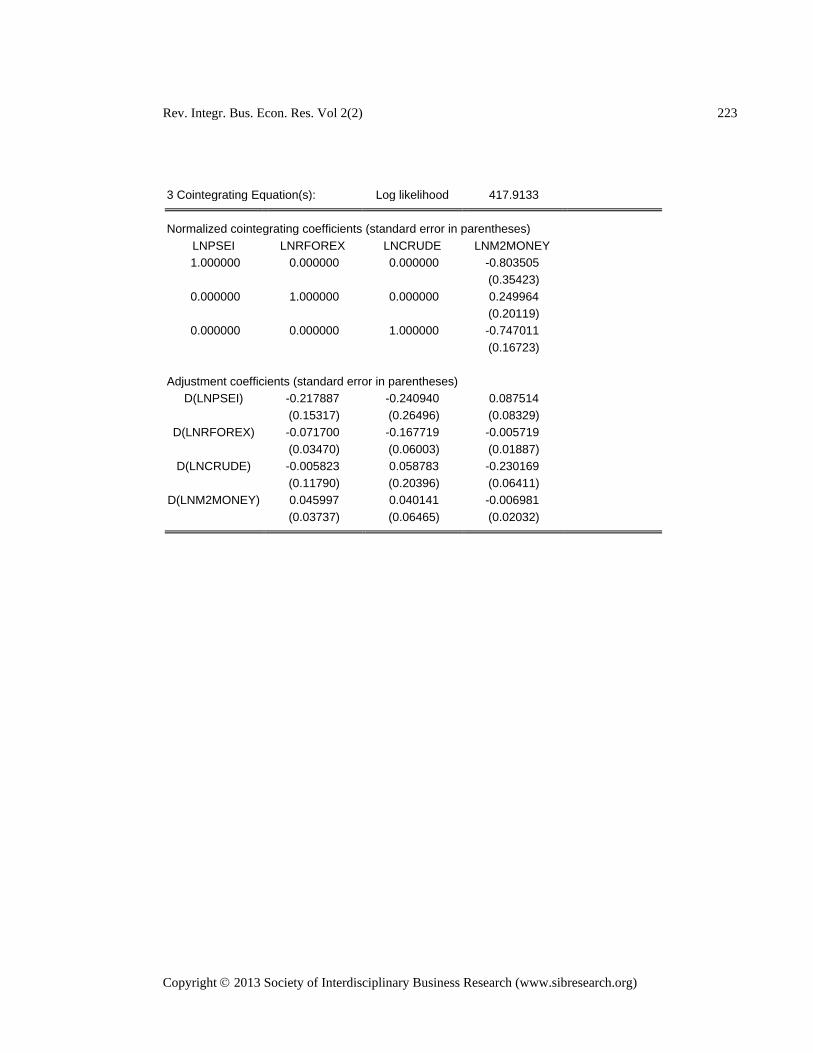
Rev. Integr. Bus. Econ. Res. Vol 2(2) 223
Copyright 2013 Society of Interdisciplinary Business Research (www.sibresearch.org)
3 Cointegrating Equation(s): Log likelihood 417.9133 Normalized cointegrating coefficients (standard error in parentheses)
LNPSEI LNRFOREX LNCRUDE LNM2MONEY 1.000000 0.000000 0.000000 -0.803505
(0.35423) 0.000000 1.000000 0.000000 0.249964
(0.20119) 0.000000 0.000000 1.000000 -0.747011
(0.16723)
Adjustment coefficients (standard error in parentheses) D(LNPSEI) -0.217887 -0.240940 0.087514
(0.15317) (0.26496) (0.08329) D(LNRFOREX) -0.071700 -0.167719 -0.005719
(0.03470) (0.06003) (0.01887) D(LNCRUDE) -0.005823 0.058783 -0.230169
(0.11790) (0.20396) (0.06411) D(LNM2MONEY) 0.045997 0.040141 -0.006981
(0.03737) (0.06465) (0.02032)

Rev. Integr. Bus. Econ. Res. Vol 2(2) 224
Copyright 2013 Society of Interdisciplinary Business Research (www.sibresearch.org)
Appendix 21. Full Results of Johansen Cointegration Test
Option 4 - Intercept and Trend in CE – No Trend in VAR
Trend assumption: Linear deterministic trend (restricted)
Unrestricted Cointegration Rank Test (Trace) Hypothesized Trace 0.05
No. of CE(s) Eigenvalue Statistic Critical Value Prob.** None * 0.305096 66.92621 63.87610 0.0271
At most 1 0.219890 41.08347 42.91525 0.0754 At most 2 0.201193 23.45268 25.87211 0.0971 At most 3 0.100291 7.503545 12.51798 0.2949
Trace test indicates 1 cointegrating eqn(s) at the 0.05 level * denotes rejection of the hypothesis at the 0.05 level **MacKinnon-Haug-Michelis (1999) p-values
Unrestricted Cointegration Rank Test (Maximum Eigenvalue) Hypothesized Max-Eigen 0.05
No. of CE(s) Eigenvalue Statistic Critical Value Prob.** None 0.305096 25.84274 32.11832 0.2400
At most 1 0.219890 17.63078 25.82321 0.4060 At most 2 0.201193 15.94914 19.38704 0.1474 At most 3 0.100291 7.503545 12.51798 0.2949
Max-eigenvalue test indicates no cointegration at the 0.05 level * denotes rejection of the hypothesis at the 0.05 level **MacKinnon-Haug-Michelis (1999) p-values
Unrestricted Cointegrating Coefficients (normalized by b'*S11*b=I): LNPSEI LNRFOREX LNCRUDE LNM2MONEY @TREND(92Q2)
-4.741774 -6.874882 5.927274 8.353442 -0.202402 2.861745 8.274009 3.072906 20.54541 -0.428645 6.651375 10.77485 1.668242 -4.555598 0.012149 -1.219567 3.514701 3.219643 7.358105 -0.132538
Continue to next page

Rev. Integr. Bus. Econ. Res. Vol 2(2) 225
Copyright 2013 Society of Interdisciplinary Business Research (www.sibresearch.org)
Unrestricted Adjustment Coefficients (alpha): D(LNPSEI) -0.008150 -0.059450 -0.012171 0.005699 D(LNRFOREX) 0.007951 0.003659 -0.007914 -0.006464 D(LNCRUDE) -0.043761 0.008195 -0.035307 0.001285
D(LNM2MONEY) -0.002875 -0.004203 0.004914 -0.009008 1 Cointegrating Equation(s): Log likelihood 406.4443 Normalized cointegrating coefficients (standard error in parentheses)
LNPSEI LNRFOREX LNCRUDE LNM2MONEY @TREND(92Q2) 1.000000 1.449854 -1.250012 -1.761670 0.042685
(0.49955) (0.35455) (1.08286) (0.02356)
Adjustment coefficients (standard error in parentheses) D(LNPSEI) 0.038648
(0.08563) D(LNRFOREX) -0.037704
(0.01989) D(LNCRUDE) 0.207503
(0.06794) D(LNM2MONEY) 0.013633
(0.02089) 2 Cointegrating Equation(s): Log likelihood 415.2597 Normalized cointegrating coefficients (standard error in parentheses)
LNPSEI LNRFOREX LNCRUDE LNM2MONEY @TREND(92Q2) 1.000000 0.000000 -3.587454 -10.75516 0.236284
(0.75136) (2.32985) (0.04661) 0.000000 1.000000 1.612191 6.203032 -0.133530
(0.41436) (1.28488) (0.02571)
Adjustment coefficients (standard error in parentheses) D(LNPSEI) -0.131482 -0.435853
(0.08921) (0.17327) D(LNRFOREX) -0.027234 -0.024394
(0.02307) (0.04481) D(LNCRUDE) 0.230956 0.368657
(0.07911) (0.15365) D(LNM2MONEY) 0.001606 -0.015009
(0.02419) (0.04698)
Continue to next page
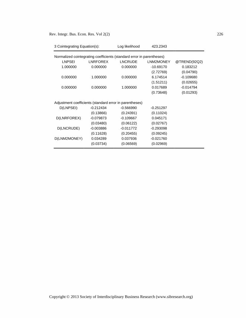
Rev. Integr. Bus. Econ. Res. Vol 2(2) 226
Copyright 2013 Society of Interdisciplinary Business Research (www.sibresearch.org)
3 Cointegrating Equation(s): Log likelihood 423.2343 Normalized cointegrating coefficients (standard error in parentheses)
LNPSEI LNRFOREX LNCRUDE LNM2MONEY @TREND(92Q2) 1.000000 0.000000 0.000000 -10.69170 0.183212
(2.72769) (0.04790) 0.000000 1.000000 0.000000 6.174514 -0.109680
(1.51211) (0.02655) 0.000000 0.000000 1.000000 0.017689 -0.014794
(0.73648) (0.01293)
Adjustment coefficients (standard error in parentheses) D(LNPSEI) -0.212434 -0.566990 -0.251297
(0.13866) (0.24391) (0.11024) D(LNRFOREX) -0.079873 -0.109667 0.045171
(0.03480) (0.06122) (0.02767) D(LNCRUDE) -0.003886 -0.011772 -0.293098
(0.11628) (0.20455) (0.09245) D(LNM2MONEY) 0.034289 0.037936 -0.021760
(0.03734) (0.06569) (0.02969)
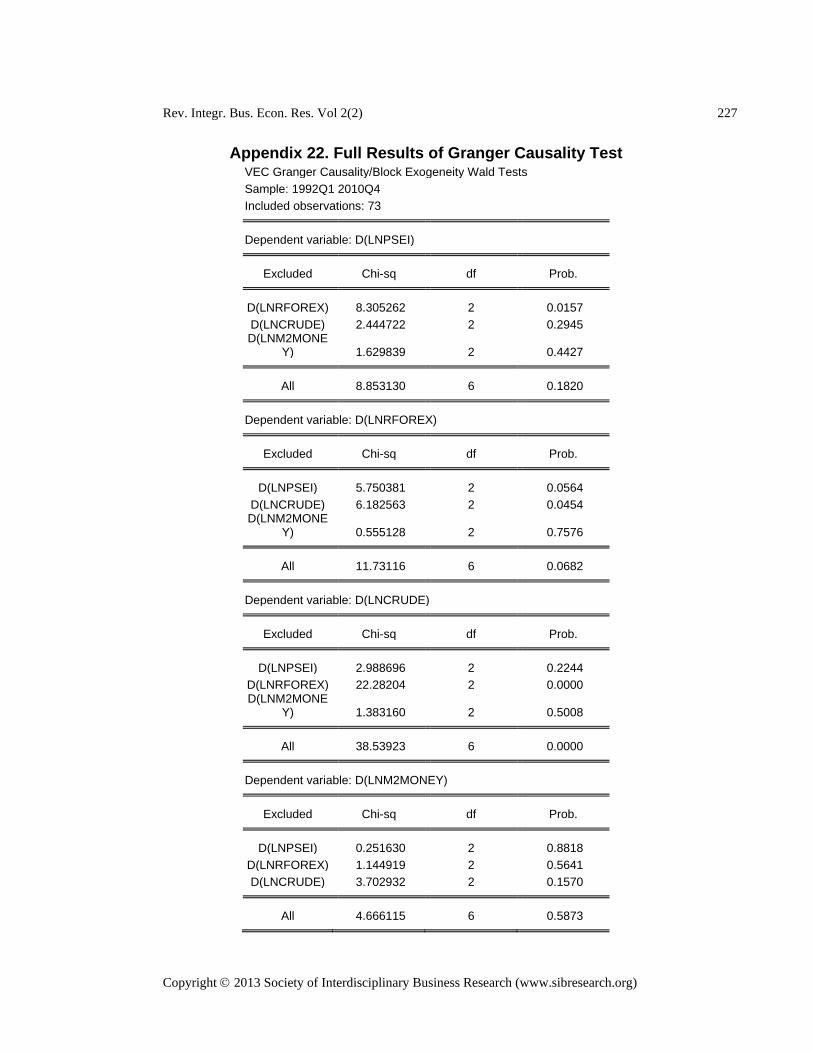
Rev. Integr. Bus. Econ. Res. Vol 2(2) 227
Copyright 2013 Society of Interdisciplinary Business Research (www.sibresearch.org)
Appendix 22. Full Results of Granger Causality Test VEC Granger Causality/Block Exogeneity Wald Tests Sample: 1992Q1 2010Q4 Included observations: 73
Dependent variable: D(LNPSEI) Excluded Chi-sq df Prob. D(LNRFOREX) 8.305262 2 0.0157
D(LNCRUDE) 2.444722 2 0.2945 D(LNM2MONE
Y) 1.629839 2 0.4427 All 8.853130 6 0.1820 Dependent variable: D(LNRFOREX) Excluded Chi-sq df Prob. D(LNPSEI) 5.750381 2 0.0564
D(LNCRUDE) 6.182563 2 0.0454 D(LNM2MONE
Y) 0.555128 2 0.7576 All 11.73116 6 0.0682 Dependent variable: D(LNCRUDE) Excluded Chi-sq df Prob. D(LNPSEI) 2.988696 2 0.2244
D(LNRFOREX) 22.28204 2 0.0000 D(LNM2MONE
Y) 1.383160 2 0.5008 All 38.53923 6 0.0000 Dependent variable: D(LNM2MONEY) Excluded Chi-sq df Prob. D(LNPSEI) 0.251630 2 0.8818
D(LNRFOREX) 1.144919 2 0.5641 D(LNCRUDE) 3.702932 2 0.1570
All 4.666115 6 0.5873