The Basics of Earthquake Location

William Menke

Lamont-Doherty Earth Observatory

Columbia University

The basic data in earthquake location is

Arrival Time, t

The time of day that a wave from the earthquake arrives at a seismograph station

The distinction between

Arrival Time: time of day something arrives

And

Travel Time: the length of time spent traveling

Is very important in earthquake location!

Arrival Time ≠Travel Time

Q: a car arrived in town after traveling for an half an hour at sixty miles an hour. Where did it start?

A. Thirty miles away

Q: a car arrived in town at half past one, traveling at sixty miles an hour. Where andwhen did it start?

A. Are you crazy?

An earthquake location has4 Parameters

x, y (epicenter)z (depth)(origin time)

Together, (x, y, z) are called the hypocenter. The fact that origin time is an unknown adds complexity to the earthquake location problem!

Suppose you contour arrival timeon surface of earth

Earthquake’s (x,y) is center of bulls-eye

but what about its depth?

Earthquake’s depth related to

curvature of arrival time at

origin

Deep

Shallow

Since origin time unknownwe have not marked it on

time axis

Fundamental data:arrival time tpi of waves

from earthquake p to station i

Wave could be either P wave or S wave. Both are used.

Fundamental Relationship

Arrival Time = Origin Time + Travel Time

tpi = p + Tpi

Traveltime Tpi along ray connecting earthquake p with station q can be calculated using ray theory

ray

earthquake p

with origin time p

Locating an earthquakerequires knowing the

earth’s seismic velocity structure

accuratelyso that traveltime can be calculatedbetween stations and hypothetical

hypocenters

examplevelocity

structure(Iceland)

in this caseassumed to

vary only with depth

Basic Principle

Best estimates of the hypocentral parameters and origin time are the ones that best predict the arrival times at all the stations.

Usually, “best predicts” means minimizingthe least-squares prediction error, E:

Ep = i [ tpiobserved – tpi

predicted ]2

where tpipredicted = p

predicted + Tpipredicted

and where Tpipredicted depends on (xp, yp, zp)

The mathematical problem is to find thehypocentral parameters,

xppredicted=(xp, yp, zp)predicted

and origin time, p

predicted

that give the best fit(which is to say, minimize the error)

But the problem is that the traveltime varies in a complicated, non-linear way with the hypocentral parameters, xp

predicted

The usual solution is to use an iterative method:

Step 1: Guess a set of hypocentral parameters, h=(xp, yp, zp, p) = (xp, , p) and use it to predict the traveltime

Step 2: Determine how much the arrival time would change if the guess were changed by a small amount, h = x, .

Step 3: Use that information to attempt to find a slightly different h that reduces the error, E.

Do steps 2 and 3 over and over again, hoping that eventually the error will become acceptably small.

It turns out that Step 2 is incredibly easy.

A small change in origin time, , simply shifts the arrival times by the same amount, t = .

The effect of a small change in location depends on the direction of the shift. A change x along the ray direction shifts the time by t=x/v. But a change perpendicular to the ray has no effect. This is Geiger’s Principle, and illustrated in the next slide.

Step 3 is pretty easy too. The trick is to realize that the equation that says the observed and predicted traveltimes are equal is now linear in the unknowns:

tpiobs = tpi

pre = p + Tpipre

= pguess + + Tpi

pre(xpguess) + (t/v)x

Or by moving two terms to the left:

tpiobs - Tpi

pre(xpguess) - p

guess = + (t/v)x

The methodology for solving a linear equation in the least-squares sense is very well known. It requires some tedious matrix algebra, so we wont discuss it here. But is routine.

but with any method, a key question is …

What can go wrong?

here are some possibilities …

Too few data …

Since there are four unknowns,you must have at least four arrival time measurements. Any fewer,

and you cannot locate the earthquake.

Bad Station Geometry …

But P and S waves from each of two stations won’t do it, because

there is a left-right ambiguity

earthquake here?

or here?

station 2

station 1

Another poor geometry …

When the stations are all to one side of the stations, the rays all leave the

source in roughly the same direction and location trades off with origin time

station 2

shallow and late

deep and early

Depending upon ray geometry, this trade-off can also involve depth and origin time

Recently, a new earthquake location method has been

developed

that instead of locating a single earthquake on the basis of its

arrival times (as above)

locates groups of earthquakes on the basis of the difference

in their arrival times

This method is often called the

Double-Difference Method

the following figures illustrate its power

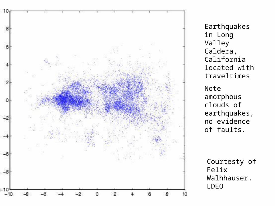
Courtesty of Felix Walhhauser, LDEO

Earthquakes in Long Valley Caldera, California located with traveltimes

Note amorphous clouds of earthquakes, no evidence of faults.

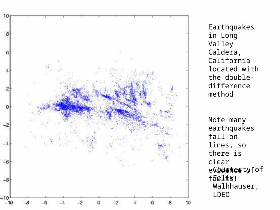
Courtesty of Felix Walhhauser, LDEO

Earthquakes in Long Valley Caldera, California located with the double-difference method

Note many earthquakes fall on lines, so there is clear evidence of faults!

The basic data in the double-difference method is the differential arrival time between two different earthquakes observed at the same station: Dtpqi = tpi - tqi

But that is another story …