The Base Strategy for ID3 Algorithm of Data Mining Using Havrda and Charvat Entropy Based on

Abstract—Data mining is used to extract the required data

from large databases [1]. The data mining algorithm is the mechanism that creates mining models [2]. To create a model, an algorithm first learns the rules from a set of data then looks for specific required patterns and trends according to those rules. The algorithm then uses the fallouts of this exploration to delineate the constraints of the mining model [2]. These constraints are then applied through the intact data set to extract the unlawful patterns and detailed statistics [2]. Decision-tree learning is one of the utmost efficacious erudition algorithms, due to its various eye-catching features: simplicity, comprehensibility, no parameters, and being able to handle mixed-type data [3]; ID3 is a simple decision tree erudition algorithm developed by Ross Quinlan (1983) [4]. This paper introduces the use of ID3 algorithm [4] of decision tree and we use Havrda and Charvat Entropy instead of Shannon Entropy [5]. By computing information we set particular property from taken data as root of tree, also sub-root by repeating the process continually, to finally build the most optimized tree. This decision tree helps to take the decision for better analysis of data. Decision tree algorithm is used to select the best path to follow in the standard division. This paper introduces the use of ID3 algorithm of decision tree. We are using Havrda and Charvat Entropy Instead of Shannon Entropy. This Decision Tree helps in taking the better decision to analyse the data.

Index Terms—Data mining, decision tree, Shanon entropy, Havrda and Charvat entropy, ID3 algorithm, knowledge-driven decisions.

I. INTRODUCTION Data mining is the technique to extract the hidden

predictive data from large databases; it is an influential technology and used by lot of companies because of very prodigious fallouts [6], [7]. Data mining is very supportive technique to analyse the forthcoming prediction with the help of historical behaviour of data and statistics, these features of data mining sanction proactive business and it is called knowledge-driven decisions. This automation, prospective scrutinizing and exploration of past events work as retrospective tool and implement a DSS (decision support system).

Data mining techniques can rapidly implement on existing

Manuscript received January 28, 2012; revised March 3, 2012. N. Mathur is with the Delhi College of Engineering, India (e-mail:

[email protected]). Sumit Kumar and Santosh Kumar are with the Department of Computer

Science and Engineering, Indian Institute of Technology Patna, Patna, India (e-mail: [email protected], [email protected]).

R. Jindal is with Delhi Technological University, India (e-mail: [email protected]).

software and hardware and intensify the quality of service of them.

A. ID3 Algorithm ID3 is a simple decision tree erudition algorithm

developed by Ross Quinlan (1983) [4]. The basic idea of ID3 algorithm is to create a decision tree of given set, by using top-down greedy search to check each attribute at every tree node. To select the most useful attribute using classification technique, we present a metric---information gain and to catch an optimal way to classify an erudite set, we need to minimize the depth of the tree. Thus, we need some function which should be able to measure the most balanced splitting. The information gain metric is such a function that we can use for efficient balanced splitting. In direction to define information gain exactly, we need to deliberate entropy. First, let’s assume that the resulting decision tree classifies instance into two classes without loss of simplification and we would call them P (positive) and N (negative). Given set S, containing these positive and negative targets, the entropy of S related to this Boolean classification is:

Entropy(S) ＝－P (positive) log2P (positive) － P (negative) log2P (negative)

P (positive): proportion of positive examples in S P (negative): proportion of negative examples in S

So concerning Points are as we discussed, to minimize the

decision tree depth; we need to select the optimal attribute for splitting the tree node, so that we can easily imply the attribute with the maximum entropy reduction. The attribute that can help in maximum entropy reduction is the optimal attribute for splitting. We define Information Gain as the predictable reduction of entropy related to specified attribute when splitting a decision tree node. The information gain, Gain(S, A) of an attribute A, Gain(S, A) ＝ Entropy(S) －Sum for v from 1 to n of (|Sv|／|S|) × Entropy (Sv).

We have to use this concept of gain to rank attributes to build decision trees where at each node is located the attribute with utmost gain among the attributes that not yet considered in the path from the root.

The purpose of this ordering is to create small decision trees so that records can be identified after only a few

The Base Strategy for ID3 Algorithm of Data Mining Using Havrda and Charvat Entropy Based on Decision

Tree

Nishant Mathur, Sumit Kumar, Santosh Kumar, and Rajni Jindal

International Journal of Information and Electronics Engineering, Vol. 2, No. 2, March 2012

253

decision tree splitting and match a hoped for plainness of the process of decision making.

B. Problem Statement Shannon Entropy finds its application in many fields. Here,

Shannon Entropy has been used in ID3 algorithm to calculate the Information Gain contained by data, which helps to make Decision Tree.

However, the results obtained from Shannon Entropy, are rather complex, have more numbers of node and leaf and Decision Rules. Thus it makes the decision making process time consuming.

Therefore, to minimize these problems, new algorithm has been proposed by modifying ID3 algorithm using Havrda and Charvat Entropy instead of Shannon Entropy

II. EVALUATION AND DEPICTION Classification is perhaps the utmost acquainted and the

most extensive data mining technique. Examples of classification application are images and pattern recognition, medical diagnosis, loan approval, detecting faults in industrial application, and classifying market trends [8]. Estimation and prediction can be view as types of classification. Prediction can classify an attribute value from a set of possible values. It is often viewed as forecasting value, while classification forecasts a discrete value.

All methodologies to perform classification assume certain acquaintance of the data. Habitually a training set is used to develop the precise parameters, those are obligatory through the technique. Training data contains a sample of input data as well as the classification assignment for the data.

The classification problem is stated as: Definition: Given a database D = {t1, t2, t3……tm} of

tuples (items, records) and a set of classe C = {c1, c2, c3…..cm} the classification problem is to define a mapping f: D-> C where ti is assigned to one class. A class, cj contain precisely those mapped to it; that is, cj = {ti /f (ti) = cj, 1<=i<=n, and t1 belong to D}

According to definition’s interpretations, classification is a mapping of the database to the set of classes. Each tuple in the database is assigned to exactly one class.

The classes that exist for a classification problem are indeed equivalence classes. In actuality, the problem usually is implemented in two phases:

1) Create a specific model by evaluating the training data. This step takes the training data as input and gives the output as the definition of the developed model. The developed model classifies the training data as accurate as possible.

2) Apply the established model in step 1 by classifying tuples from the target database.

A. Depiction of Decision Tree and ID3 Algorithm In this section, we define the ID3 Algorithm and the depict

role of decision tree. The Decision Trees algorithm creates hierarchical structure of classification rules “If ... Then ...” looking like a tree. To choose which type to assign for an object or state, we have to answer the questions, standing in the branches of the tree, starting from the root. The questions look like this: “Is the value of the parameter A greater than

Х?” If the answer is positive, a pass to the right performs, if it is negative – to the left; then a question related to the new branch follows. In following illustration, information about customers was produced, including their debt level, income level, what type of occupation they had, and whether they represented a good or bad credit risk

A decision Tree consists of 3 types of nodes: 1) Decision nodes - commonly represented by squares 2) Change nodes - represented by circles 3) End nodes - represented by triangles

Fig. 1. Decision tree showing types of nodes.

Decision trees are used in operations research, decision analysis, to help identify a strategy, calculating conditional probabilities etc.

In decision analysis, a "decision tree”, is used as a visual and analytical decision support tool, where the predictable value of competing options are deliberate.

Decision trees have traditionally been created manually, as shown in Fig. 1.

III. ISSUES, IMPLEMENTATION AND RESULTS OF PROPOSED ALGORITHM USING HAVRDA AND CHARVAT

ENTROPY The ID3 algorithm is used to build a decision tree, given a

set of non-categorical attributes C1, C2, .., Cn, the categorical attribute C, and a training set T of records.

Algorithm 1) Function ID3 (R: a set of non-categorical attributes,

2) C: the categorical attribute,

3) S: a training set) returns a decision tree;

4) begin

5) If S is empty, return a single node with value Failure;

6) If S consists of records all with the same value for the categorical attribute,

7) Return a single node with that value;

8) If R is empty, then return a single node with as value the most frequent of the values of the categorical attribute that are found in records of S; [note that then there will be errors, that is, records that will be improperly classified];

9) Let D be the attribute with largest Gain (D,S)

10) Among attributes in R;

11) Let {dj| j=1,2, .., m} be the values of attribute D;

12) Let {Sj| j=1,2, .., m} be the subsets of S consisting respectively of records with value dj for attribute D;

13) Return a tree with root labeled D and arcs labelled.


254

14) d1, d2, .., dm going respectively to the trees

15) ID3(R-{D}, C, S1), ID3(R-{D}, C, S2), .., ID3(R-{D}, C, Sm);

16) end ID3;

A. Entropy as Information Content Entropy is demarcated in the perspective of a probabilistic

model. Independent fair penny tosses have Entropy of 1 bit per flip. A source that always produces a long string of B's has Entropy of 0, since the next character will always be a 'B'. The entropy rate of a data source means the average number of bits per sign needed to encode it.

B. Definition and Role of Havrda and Charvat Entropy Let P = (p1, p2 …pn) be a probability distribution, p denotes

the probability mass function of X and α is its inherent parameter [13]. Then Havrda and Charvat [12] gave the entropy measure by formula shown under

1

1( ) ( 1)1

nai

i

h p Xa =

= −− ∑

This formula calculates Entropy. To avoid deduced solution in decision tree making process, Havrda and Charvat entropy based ID3 algorithm is proposed which gives good solution in reasonable time. Such algorithm can give short and fast decision for supply of good in company.

C. Havrda and Charvat Entropy in ID3 algorithm The measure of tree component is one of the most

important problems of ID3. Such problems occur when we have to take decision for who will be the root of the tree. So to find one we have to calculate first the needed information, so for needed information we divided our data [2] into category for which we are making tree here we divided data according to customer type, here taking sample data into two parts: Sing_Customer (B) and Normal_Customer (N).

D. Implementation and Analysis of Proposed Algorithm

TABLE I: INFORMATION OF CUSTOMER DISPATCH GOODS

The summarized data of customer dispatch information in

a section period (one month) from an information system

database of a 3PL, which including 19 items in this sample data set. In this example [13], all sample data is divided by Customer Type (CT) into two classes, which are Sign_Customer (B) and Normal_Customer (N) respectively, and has four properties: Freight Fee, Payment, Weight, and Dispatch Time. On the one hand, the summarizing data is integrated data from different sections and different consignment nodes. On the other hand, it is the process of generalizing the sample data, namely, the low level data are substituted by high level convenient to data mining. The values of these four properties are: Freight Fee (<100,100~1000, >1000); Payment (<100, 100~2000, <2000); Weight (<100 kg, 100 kg~500 kg, >500 kg); Dispatch Times (<5, 5~20, >20) [2]. The meanings of these properties are: The freight fee is paid by customer for the transport cost; the payment is Transportation Company bring the money of the goods from the receiver to dispatcher; the weight is measured by kilogram; the dispatch time is the sum times during the summarized period.

We can calculate needed information by taking probability of customer type here we B class have 8 items and N has 11 items. Therefore, needed information gain of taken sample by putting α=0.25, 0.50, 0.75 etc in Havrda and Charvat formula.

Assuming α=0.25

The needed information gain will be .25 0.258 11 1

19 190.677(8,11) 0.903

1 0.25 0.75I

⎡ ⎤⎛ ⎞ ⎛ ⎞+ −⎢ ⎥⎜ ⎟ ⎜ ⎟⎝ ⎠ ⎝ ⎠⎢ ⎥⎣ ⎦

= = =−

Then we divided the sample data by four property, freight fee, payment, weight, and dispatch time respectively. Therefore the corresponding anticipated information of sample data are:

E (Freight fee) =

.25 0.259 2 7 119 9 9

0.75

⎡ ⎤⎛ ⎞ ⎛ ⎞+ −⎢ ⎥⎜ ⎟ ⎜ ⎟⎝ ⎠ ⎝ ⎠⎢ ⎥⎣ ⎦

+

.25 0.257 4 3 119 7 7

0.75

⎡ ⎤⎛ ⎞ ⎛ ⎞+ −⎢ ⎥⎜ ⎟ ⎜ ⎟⎝ ⎠ ⎝ ⎠⎢ ⎥⎣ ⎦

+

.253 3 119 3

0.75

⎡ ⎤⎛ ⎞ −⎢ ⎥⎜ ⎟⎝ ⎠⎢ ⎥⎣ ⎦

=0.395 + 0.333 + 0 = 0.728

E (Payment) =

.25 0.2512 6 6 119 12 12

0.75

⎡ ⎤⎛ ⎞ ⎛ ⎞+ −⎢ ⎥⎜ ⎟ ⎜ ⎟⎝ ⎠ ⎝ ⎠⎢ ⎥⎣ ⎦

+

.25 0.254 1 3 119 4 4

0.75

⎡ ⎤⎛ ⎞ ⎛ ⎞+ −⎢ ⎥⎜ ⎟ ⎜ ⎟⎝ ⎠ ⎝ ⎠⎢ ⎥⎣ ⎦

+

.25 0.253 2 1 119 3 3

0.75

⎡ ⎤⎛ ⎞ ⎛ ⎞+ −⎢ ⎥⎜ ⎟ ⎜ ⎟⎝ ⎠ ⎝ ⎠⎢ ⎥⎣ ⎦

= 0.574 + 0.179 + 0,139 = 0.893

E (Weight) =

.25 0.2511 2 9 119 11 11

0.75

⎡ ⎤⎛ ⎞ ⎛ ⎞+ −⎢ ⎥⎜ ⎟ ⎜ ⎟⎝ ⎠ ⎝ ⎠⎢ ⎥⎣ ⎦

+

.25 0.255 4 1 119 5 5

0.75

⎡ ⎤⎛ ⎞ ⎛ ⎞+ −⎢ ⎥⎜ ⎟ ⎜ ⎟⎝ ⎠ ⎝ ⎠⎢ ⎥⎣ ⎦

+

.25 0.253 2 1 119 3 3

0.75

⎡ ⎤⎛ ⎞ ⎛ ⎞+ −⎢ ⎥⎜ ⎟ ⎜ ⎟⎝ ⎠ ⎝ ⎠⎢ ⎥⎣ ⎦

= 0.466 + 0.216 + 0.139 = 0.822


255

E (Time) =

.25 0.257 1 6 119 7 7

0.75

⎡ ⎤⎛ ⎞ ⎛ ⎞+ −⎢ ⎥⎜ ⎟ ⎜ ⎟⎝ ⎠ ⎝ ⎠⎢ ⎥⎣ ⎦

+

.25 0.258 4 4 119 8 8

0.75

⎡ ⎤⎛ ⎞ ⎛ ⎞+ −⎢ ⎥⎜ ⎟ ⎜ ⎟⎝ ⎠ ⎝ ⎠⎢ ⎥⎣ ⎦

+

.25 0.254 3 1 119 4 4

0.75

⎡ ⎤⎛ ⎞ ⎛ ⎞+ −⎢ ⎥⎜ ⎟ ⎜ ⎟⎝ ⎠ ⎝ ⎠⎢ ⎥⎣ ⎦

= 0.283 + 0.383 + 0.179 = 0.845

Corresponding information gains are:

Gain (Freight fee) = I (S1, S2) – E (Freight fee)

= 0.903 – 0.728 = 0.175

Gain (Payment) = I (S1, S2) – E (Payment)

= 0.903 – 0.893 = 0.011

Gain (Weight) = I (S1, S2) – E (Weight)

= 0.903 – 0.822 = 0.082

Gain (Time) = I (S1, S2) – E (Time)

= 0.903 – 0.845 = 0.058

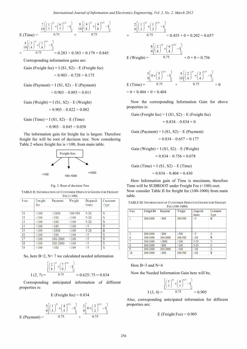
The information gain for freight fee is largest. Therefore freight fee will be root of decision tree. Now considering Table 2 where freight fee is <100, from main table.

Fig. 2. Root of decision Tree

TABLE II: INFORMATION OF CUSTOMER DISPATCH GOODS FOR FREIGHT FEE (<100)

So, here B=2, N= 7 we calculated needed information

I (2, 7) =

.25 0.252 7 19 9

0.75

⎡ ⎤⎛ ⎞ ⎛ ⎞+ −⎢ ⎥⎜ ⎟ ⎜ ⎟⎝ ⎠ ⎝ ⎠⎢ ⎥⎣ ⎦

= 0.625/.75 = 0.834

Corresponding anticipated information of different properties is:

E (Freight fee) = 0.834

E (Payment) =

.25 0.255 1 4 19 5 5

0.75

⎡ ⎤⎛ ⎞ ⎛ ⎞+ −⎢ ⎥⎜ ⎟ ⎜ ⎟⎝ ⎠ ⎝ ⎠⎢ ⎥⎣ ⎦

+

0.252 20 19 2

0.75

⎡ ⎤⎛ ⎞+ −⎢ ⎥⎜ ⎟⎝ ⎠⎢ ⎥⎣ ⎦

+

.25 0.252 1 1 19 2 2

0.75

⎡ ⎤⎛ ⎞ ⎛ ⎞+ −⎢ ⎥⎜ ⎟ ⎜ ⎟⎝ ⎠ ⎝ ⎠⎢ ⎥⎣ ⎦

= 0.455 + 0 + 0.202 = 0.657

E (Weight) =

.25 0.258 2 6 19 8 8

0.75

⎡ ⎤⎛ ⎞ ⎛ ⎞+ −⎢ ⎥⎜ ⎟ ⎜ ⎟⎝ ⎠ ⎝ ⎠⎢ ⎥⎣ ⎦

+ 0 + 0 = 0.756

E (Time) =

0.255 50 19 5

0.75

⎡ ⎤⎛ ⎞+ −⎢ ⎥⎜ ⎟⎝ ⎠⎢ ⎥⎣ ⎦

+

.25 0.254 2 2 119 4 4

0.75

⎡ ⎤⎛ ⎞ ⎛ ⎞+ −⎢ ⎥⎜ ⎟ ⎜ ⎟⎝ ⎠ ⎝ ⎠⎢ ⎥⎣ ⎦

+ 0

= 0 + 0.404 + 0 = 0.404

Now the corresponding Information Gain for above properties is:


= 0.834 – 0.834 = 0


= 0.834 – 0.657 = 0.177


= 0.834 – 0.756 = 0.078


= 0.834 – 0.404 = 0.430

Here Information gain of Time is maximum, therefore Time will be SUBROOT under Freight Fee (<100) root. Now consider Table II for freight fee (100-1000) from main table. TABLE III: INFORMATION OF CUSTOMER DISPATCH GOODS FOR FREIGHT

FEE (100-1000)

Here B=3 and N=4

Now the Needed Information Gain here will be,

I (3, 4) =

.25 0.253 4 17 7

0.75

⎡ ⎤⎛ ⎞ ⎛ ⎞+ −⎢ ⎥⎜ ⎟ ⎜ ⎟⎝ ⎠ ⎝ ⎠⎢ ⎥⎣ ⎦

= 0.905

Also, corresponding anticipated information for different properties are:

E (Freight Fee) = 0.905

Freight fees

>1000 <100 100-1000


256

E (Payment) =

.25 0.254 2 2 17 4 4

0.75

⎡ ⎤⎛ ⎞ ⎛ ⎞+ −⎢ ⎥⎜ ⎟ ⎜ ⎟⎝ ⎠ ⎝ ⎠⎢ ⎥⎣ ⎦

+

.25 0.252 1 1 17 2 2

0.75

⎡ ⎤⎛ ⎞ ⎛ ⎞+ −⎢ ⎥⎜ ⎟ ⎜ ⎟⎝ ⎠ ⎝ ⎠⎢ ⎥⎣ ⎦

+ 0.251 10 1

7 10.75

⎡ ⎤⎛ ⎞+ −⎢ ⎥⎜ ⎟⎝ ⎠⎢ ⎥⎣ ⎦

= 0.519 + 0.259 + 0 = 0.778

E (Weight) =

0.253 30 17 3

0.75

⎡ ⎤⎛ ⎞+ −⎢ ⎥⎜ ⎟⎝ ⎠⎢ ⎥⎣ ⎦

+

0.253 30 17 3

0.75

⎡ ⎤⎛ ⎞+ −⎢ ⎥⎜ ⎟⎝ ⎠⎢ ⎥⎣ ⎦

+ 0.251 1 1

7 10.75

⎡ ⎤⎛ ⎞ −⎢ ⎥⎜ ⎟⎝ ⎠⎢ ⎥⎣ ⎦

= 0 + 0 + 0 = 0

E (Time) =

.25 0.252 1 1 17 2 2

0.75

⎡ ⎤⎛ ⎞ ⎛ ⎞+ −⎢ ⎥⎜ ⎟ ⎜ ⎟⎝ ⎠ ⎝ ⎠⎢ ⎥⎣ ⎦

+

.253 3 17 3

0.75

⎡ ⎤⎛ ⎞ −⎢ ⎥⎜ ⎟⎝ ⎠⎢ ⎥⎣ ⎦

+ .252 2 1

7 20.75

⎡ ⎤⎛ ⎞ −⎢ ⎥⎜ ⎟⎝ ⎠⎢ ⎥⎣ ⎦

= 0.638 + 0 + 0 = 0.638

The corresponding information gains are:


= 0


= 0.905 – 0.778 = 0.127


= 0.905 – 0 = 0.905


= 0.905 – 0.638 = 0.265

Information Gain for Weight is largest, so it will be sub root, under Freight fee (100-1000) category.

Now Consider table for Freight fee (>100) TABLE IV: INFORMATION OF CUSTOMER DISPATCH GOODS FOR FREIGHT

FEE (>1000)

From Table IV we can conclude that under freight fee

(100-1000) sub root will be PAYMENT where for it <100 customers will be B type only. Same way we will conclude for sub root weight under (freight fee 100-1000 only) from table we can observe that for sub root weight <100 customer is N type, for 100-1000 customer is B type and for weight >500 customer is N type. From above calculation and observation we have drawn the following tree.

E. Generation of Decision Tree

Fig. 3. Output in decision tree format.

F. Output in Command Prompt of ‘C’ Compilation

Fig. 4. Output in command prompt of ‘C’ compilation.

IV. CONCLUSION Data mining as a technology can be used to analyze the

customer data to find their exact need. This will help us to give more value to customer by increasing their information, also help in providing high quality services to them by understanding them. The decision tree tells what customers want the most. In this thesis ID3 algorithm is used, but modification is done. Instead of using Shannon Entropy, Havrda and Charvat Entropy has been used to find the information of different properties which is used as the node of decision tree. This modification has reduced the size of tree as well as decreased the rules, which will help to understand customer characteristics by which company growth and profit can be increased. I have proposed a new algorithm, i.e. instead of Shannon entropy we have used the Havrda and Charvat entropy ,as a result I can conclude that for lower value of alpha (α)=0.25, tree is small and less complex as compared to the use of Shannon entropy. As


257

conclusion I can say that if we want to get less number of node and leaf in a tree and to make it more effective and less complex, we can use the Havrda and Charvat entropy instead of Shannon entropy and value of alpha (α) less than one will give decision tree with less number of nodes.

V. SCOPE FOR FUTURE WORK In this research, the value of alpha (α) has been put as 0.25,

but for further research we can take varying value of alpha (α) which may give different trees.

Various values of α have already been put in this study i.e. alpha (α) = 0.5, 0.75, 0.99, 5, 10, 100 which gave same tree as in the case of alpha (α) = 0.25. But, it has been observed that in case of α = 2, 3, 4 the tree turned out to be different with more number of leaf and high complexities.

Also, Instead of using Havrda and Charvat Entropy, Different Entropy can also be used for further research like Arimoto, Sharma-Mittal, Taneja, Sharma-Taneja, Ferreri, Sanťanna—Taneja ,Picard, Aczel-Daróczy.

REFERENCES [1] E. Thomas, “Data mining: definitions and decision tree examples,”

Stony Brook, State University Of Newyork. [2] Data Mining Algorithms (Analysis Services - Data Mining). [Online].

Available:http://technet.microsoft.com/en-us/library/ms175595.aspx [3] J. Su and H. Zhang, “A Fast Decision Tree Learning Algorithm,”

Faculty of Computer Science, University of New Brunswick, NB, Canada, E3B 5A3.

[4] W. Peng, J. Chen, and H. Zhou, “An Implementation of ID3 -- decision Tree Learning Algorithm,” University of New South Wales, School of Computer Science & Engineering, Sydney, NSW 2032, Australia.

[5] C. F. L. Lima, F. M. de Assis, C. P. de Souza, “Decision Tree based on Shannon, Rényi and Tsallis Entropies for Intrusion Tolerant Systems,” Federal Institute of Maranhão Maracanã Campus São Lu´ıs, MA – Brazil, Federal University of Campina Grande Campina Grande, PB – Brazil, Federal University of Para´ıba João Pessoa, PB – Brazil: Published in The Fifth International Conference on Internet Monitoring and Protection.

[6] J. Han and M. Kamber, “Data Mining: Concepts and Techniques (2nd edition),” Morgan Kaufmann Publishers, 2006

[7] J. R. Quinlan, “C4.5: Programs for Machine Learning,” Morgan Kaufmann Publishers, Inc., 1993.

[8] M. Lee, Y. J. Kim, Y.-M. Kim, S. Cheong, and S. Song, “Classifying Bio-Chip Data using an Ant Colony System Algorithm,” International Journal of Engineering and Applied Sciences vol. 2, no. 2, 2006

[9] T. M. Cover and P. E. Hart, “Nearest neighbor pattern classification,” IEEE transactions on information theory vol. 13, issue 1, pp. 21-27, January, 1967.

[10] L. Breiman, J. Friedman, L. Olshen, and J. Stone, “Classification and Regression trees. Wadsworth Statistics/Probability series,” CRC press Boca Raton, Florida, USA, 1984.

[11] W. Peng, J. Chen, and H. Zhou. An Implementation of ID3 Decision Tree Learning Algorithm. [Online]. Available: web.arch.usyd.edu.au/wpeng/DecisionTree2.pdf

[12] T. Chen, B. C. Vemuri, A. Rangarajan, S. J. Eisenschenk, Group-Wise Point-Set Registration Using a Novel CDF-Based Havrda-Charvát Divergence.

[13] Q. Wang, Y. Wu, J. Xiao, and G. Pan, “The Applied Research Based on Decision Tree of Data Mining In Third-Party Logistics. Automation and Logistics,” presented at 2007 IEEE International Conference on 08 October 2007, Jinan.

Mr. Nishant Mathur received M.Tech (Computer Science and Engineering) degree from Delhi College of Engineering.

Mr. Sumit Kumar received M.Tech (Computer Science and Engineering) degree from Indian Institute of Technology Guwahati then He joined Indian Institute of Technology Patna as Research Fellow in Department of Computer Science and Engineering.

Mr. Santosh Kumar received M.Tech (Computer Science and Engineering) degree from Indian Institute of Technology Guwahati then he joined Indian Institute of Technology Guwahati as Junior Project Fellow in Department of Computer Science and Engineering.

Mrs. Rajni Jindal is M.C.A., M.E.,SMIEEE , MWIE, LMISTE, LMCSI. Her specialized fields are Database Systems, Data Mining and Operating Systems. She published several research papers in reputed conferences & Journals. She is Assistant Professor at Delhi Technological University ( Formerly Delhi College of Engineering).


258

The Base Strategy for ID3 Algorithm of Data Mining Using Havrda and Charvat Entropy Based on

Documents

Transcript of The Base Strategy for ID3 Algorithm of Data Mining Using Havrda and Charvat Entropy Based on