INDIAN INSTITUTE OF TECHNOLOGY KHARAGPUR

Reinforcement LearningLearning from rewards

COURSE: CS60045

1

Pallab DasguptaProfessor, Dept. of Computer Sc & Engg

Adapted from Lecture Slides of Prof Max Welling, and Tom Michell’s book

Overview

• Supervised Learning: Immediate feedback (labels provided for every input).

• Unsupervised Learning: No feedback (no labels provided).

• Reinforcement Learning: Delayed scalar feedback (a number called reward).

• RL deals with agents that must sense and act upon their environment. • This is combines classical AI and machine learning techniques.• It the most comprehensive problem setting.

• Examples:• A robot cleaning my room and recharging its battery• Robot-soccer• How to invest in shares• Modeling the economy through rational agents• Learning how to fly a helicopter• Scheduling planes to their destinations

… and so on

The RL Framework

• more general than supervised / unsupervised learning• learn from interaction with environment to achieve a goal

environment

agentActionReward,

New state

Your action influences the state of the world which determines its reward

Challenges

• The outcome of your actions may be uncertain

• You may not be able to perfectly sense the state of the world

• The reward may be stochastic

• The reward may be delayed (for example, finding food in a maze)

• You may have no clue (model) about how the world responds to your actions

• You may have no clue (model) of how rewards are being paid off

• The world may change while you try to learn it

• How much time do you need to explore uncharted territory before you exploit what you have learned?

environment

agentActionReward,

New state

The Task

• To learn an optimal policy that maps states of the world to actions of the agent.

• For example: If this patch of room is dirty, I clean it. If my battery is empty, I recharge it.

• What is it that the agent tries to optimize?

Answer: The total future discounted reward:

Note that immediate reward is worth more than future reward.What would happen to a mouse in a maze with γ = 0 ?

: S Aπ →

21 2

0

( ) ...

0 1

t t t t

it i

i

V s r r r

r

π γ γ

γ γ

+ +

∞

+=

= + + +

= ≤ <∑

Value Function

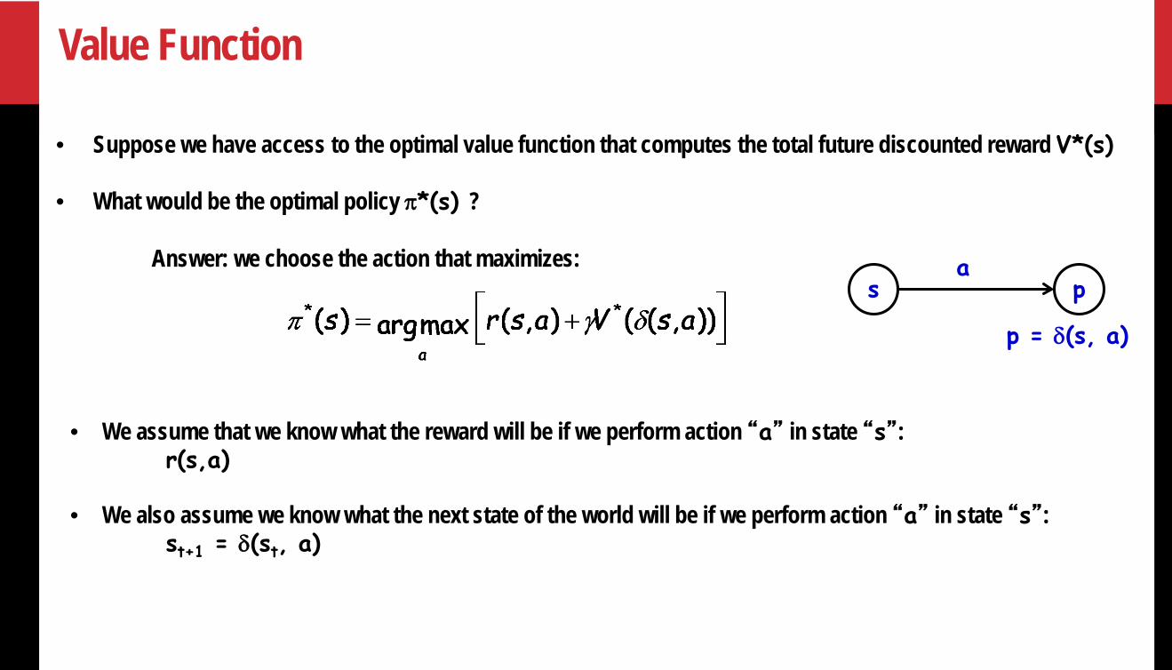
• Suppose we have access to the optimal value function that computes the total future discounted reward V*(s)

• What would be the optimal policy π*(s) ?

Answer: we choose the action that maximizes:

• We assume that we know what the reward will be if we perform action “a” in state “s”: r(s,a)

• We also assume we know what the next state of the world will be if we perform action “a” in state “s”: st+1 = δ(st, a)

s pa

p = δ(s, a)

Example 1

• Consider some complicated graph, and we would like to find the shortest path from a node Si to a goal node G.

• Traversing an edge will incur costs – this is the edge weight.

• The value function encodes the total remaining distance to the goal node from any node s, that is: V(s) = “1 / distance” to goal from s.

• If you know V(s), the problem is trivial. You simply choose the node that has highest V(s).

Si

G

Example 2: Find your way to the goal

r(s,a) : immediate reward values V*(s) : values

γ = 0.9

Therefore for the bottom left square:0 + (0.9 x 0) + (0.92 x 100) = 81

One optimal policy

Can you find the others?

The notion of Q-Function

• One approach to RL is then to try to estimate V*(s)• We may use the Bellman Equation:

• However, this approach requires you to know r(s,a) and δ(s,a)

• This is unrealistic in many real problems because the state space may not be known. For example, what is the reward if a robot is exploring Mars and decides to take a right turn?

• Fortunately we can circumvent this problem by exploring and experiencing how the world reacts to our actions. We need to learn the values of r(s,a) and δ(s,a)

*

*

argmax( ) ( , )

( ) ( , )maxa

a

s Q s a

V s Q s a

π =

=

• We want a function that directly learns good state-action pairs, that is, what action should be taken in this state.

• We call this Q(s,a).

• Given Q(s,a) it is now trivial to execute the optimal policy, without knowing r(s,a) and δ(s,a).

• We have:

Example 2 (revisited)

Note that: *

*

argmax( ) ( , )

( ) ( , )maxa

a

s Q s a

V s Q s a

π =

=

V*(s) : values Q(s,a) : values

One optimal policy

Q-Learning

Now:

This still depends on r(s,a) and δ(s,a)

*

*

argmax( ) ( , )

( ) ( , )maxa

a

s Q s a

V s Q s a

π =

=

Imagine the robot is exploring its environment, trying new actions as it goes.

• At every step it receives some reward “r”, and it observes the environment change into a new state s′ for action a.

• How can we use these observations, (s,a,s′,r) to learn a model?

where: s′ = δ(s,a)

Q-Learning

• This equation continually estimates Q at state s consistent with an estimate of Q at state s′, one step in the future.

• Note that s′ is closer to the goal, and hence more “reliable”, but still an estimate itself.

• Updating estimates based on other heuristics is called bootstrapping.

• We do an update after each state-action pair, that is, we are learning online!

• We are learning useful things about explored state-action pairs. These are typically most useful because they are likely to be encountered again.

• Under suitable conditions, these updates can actually be proved to converge to the real answer.

where: s′ = δ(s,a)

Example: One step of Q-Learning

Q-learning propagates Q-estimates 1-step backwards

1 2'

ˆ ˆ( , ) ( , ')max

0 0.9 max{66,81,100}90

righta

Q s a r Q s aγ← +

← +

←

max{63,81,100}

Getting stuck in local optima

• It is very important that the agent does not simply follow the current policy when learning Q. (off-policy learning).

• The reason is that you may get stuck in a suboptimal solution, that is, there may be other solutions out there that you have never seen.

• Hence it is good to try new things so now and then.• For example, we could use something like:

• Recall simulated annealing• If T is large lots of exploring, if T is small, follow current policy.• One can decrease T over time.

ˆ( , )/( | ) eQ s a TP a s ∝

Improvements

• One can trade-off memory and computation by cashing (s,a,s′,r) for observed transitions. After a while, as Q(s′,a′) has changed, you can “replay” the update:

• One can actively search for state-action pairs for which Q(s,a) is expected to change a lot (Prioritized Sweeping).

• One can do updates along the sampled path much further back than just one step. We have studied TD with one step, but we could do TD with many steps, called TD(λ). (TD = Temporal Difference Learning).

Extensions

• To deal with stochastic environments, we need to maximize expected future discounted reward:

• Often the state space is too large to deal with all states. In this case we need to learn a function:

• Neural network with back-propagation have been quite successful

( , ) ( , )Q s a f s aθ≈

Monte Carlo Policy Evaluation

We wish to estimate Vπ(s)

= expected return starting from s and following π• estimate is average of observed returns in state s

First-visit MC

• average returns following the first visit to state s

s ss0 +1 -2 0 +1 -3 +5 R1(s) = +2

s0

s0

s0

s0

s0

R2(s) = +1R3(s) = -5

R4(s) = +4

Vπ(s) ≈ (2 + 1 – 5 + 4)/4 = 0.5

• Based on experience or simulated experience

• Averaged sample returns

• Defined only for episodic tasks

Monte Carlo Control

• We wish to improve the policy as we explore• Estimate Qπ(s,a)

• MC Control: • update after each episode

• A problem: greedy policy won’t explore all actions

• ε-greedy policy

• with probability 1-ε perform the optimal/greedy action• with probability ε perform a random action

Temporal Difference Learning

Combines ideas from MC and DP

• like MC: learn directly from experience (don’t need a model)

• like DP: learn from values of successors

MC:

• Has to wait until the end of episode to update

Simplest TD

• update after every step, based on the successor

EXAMPLE

Consider the following 8 episodes:A – 0, B – 0 B – 1 B – 1 B – 1B – 1 B – 1 B – 1 B – 0

MC and TD agree on V(B) = 3/4

MC: V(A) = 0• converges to values that minimize the

error on training data

TD: V(A) = 3/4• converges to ML estimate of the Markov

process

A Br = 0100%

r = 175%

r = 025%

Designing Rewards

robot in a maze• episodic task, not discounted, +1 when out, 0 for each step

chess• GOOD: +1 for winning, -1 losing• BAD: +0.25 for taking opponent’s pieces

• high reward even when you loose

rewards• rewards indicate what we want to accomplish• NOT how we want to accomplish it

shaping• positive reward often very “far away”• rewards for achieving sub-goals (domain knowledge)• Also: adjust initial policy or initial value function

Reward Hacking is a problem

Conclusion

• Reinforcement learning addresses a very broad and relevant question: How can we learn to survive in our environment?

• We have looked at Q-learning, which simply learns from experience.• No model of the world is needed.

• We made simplifying assumptions: e.g. state of the world only depends on last state and action. This is the Markov assumption. The model is called a Markov Decision Process (MDP).

• There are many extensions to speed up learning.

• There have been many successful real world applications.