The association of urban greenness and walking behaviorUsing google street view and deep learning techniques to estimate residents’ exposure tourban greennessLu, Yi

Published in:International Journal of Environmental Research and Public Health

Published: 01/08/2018

Document Version:Final Published version, also known as Publisher’s PDF, Publisher’s Final version or Version of Record

License:CC BY

Publication record in CityU Scholars:Go to record

Published version (DOI):10.3390/ijerph15081576

Publication details:Lu, Y. (2018). The association of urban greenness and walking behavior: Using google street view and deeplearning techniques to estimate residents’ exposure to urban greenness. International Journal of EnvironmentalResearch and Public Health, 15(8), [1576]. https://doi.org/10.3390/ijerph15081576

Citing this paperPlease note that where the full-text provided on CityU Scholars is the Post-print version (also known as Accepted AuthorManuscript, Peer-reviewed or Author Final version), it may differ from the Final Published version. When citing, ensure thatyou check and use the publisher's definitive version for pagination and other details.

General rightsCopyright for the publications made accessible via the CityU Scholars portal is retained by the author(s) and/or othercopyright owners and it is a condition of accessing these publications that users recognise and abide by the legalrequirements associated with these rights. Users may not further distribute the material or use it for any profit-making activityor commercial gain.Publisher permissionPermission for previously published items are in accordance with publisher's copyright policies sourced from the SHERPARoMEO database. Links to full text versions (either Published or Post-print) are only available if corresponding publishersallow open access.

Take down policyContact lbscholars@cityu.edu.hk if you believe that this document breaches copyright and provide us with details. We willremove access to the work immediately and investigate your claim.

Download date: 14/03/2022

International Journal of

Environmental Research

and Public Health

Article

The Association of Urban Greenness and WalkingBehavior: Using Google Street View and DeepLearning Techniques to Estimate Residents’ Exposureto Urban Greenness

Yi Lu 1,2 ID

1 Department of Architecture and Civil Engineering, City University of Hong Kong, Hong Kong, China;yilu24@cityu.edu.hk

2 City University of Hong Kong Shenzhen Research Institute, Shenzhen 518057, China

Received: 4 June 2018; Accepted: 23 July 2018; Published: 25 July 2018�����������������

Abstract: Many studies have established that urban greenness is associated with better healthoutcomes. Yet most studies assess urban greenness with overhead-view measures, such as park area ortree count, which often differs from the amount of greenness perceived by a person at eye-level on theground. Furthermore, those studies are often criticized for the limitation of residential self-selectionbias. In this study, urban greenness was extracted and assessed from profile view of streetscapeimages by Google Street View (GSV), in conjunction with deep learning techniques. We also exploreda unique research opportunity arising in a citywide residential reallocation scheme of Hong Kong toreduce residential self-selection bias. Two multilevel regression analyses were conducted to examinethe relationships between urban greenness and (1) the odds of walking for 24,773 public housingresidents in Hong Kong, (2) total walking time of 1994 residents, while controlling for potentialconfounders. The results suggested that eye-level greenness was significantly related to higher oddsof walking and longer walking time in both 400 m and 800 m buffers. Distance to the closest MassTransit Rail (MTR) station was also associated with higher odds of walking. Number of shops wasrelated to higher odds of walking in the 800 m buffer, but not in 400 m. Eye-level greenness, assessedby GSV images and deep learning techniques, can effectively estimate residents’ daily exposure tourban greenness, which is in turn associated with their walking behavior. Our findings apply to theentire public housing residents in Hong Kong, because of the large sample size.

Keywords: urban greenness; eye-level greenness; street greenness; physical activity; walking

1. Background

According to the biophilia hypothesis, people possess a genetically-based tendency to affiliate withnature [1]. Indeed, recent studies have established that urban residents living in the neighborhoodswith higher amount of urban greenness, comprising of parks, landscaped streets and open greenspaces,tend to have better health outcomes, such as reduced long-term stress [2], increased recovery speedafter surgery [3], improved mood [4], healthier weight outcomes [5], lower risk of chronic diseases [6],and enhanced health-related quality of life [7].

Though the health benefits of urban greenness have been well-documented, the causalmechanisms are less clear. It has been suggested that exposure to urban greenness may link tophysical and psychological benefits through different intermediate effects: through facilitating socialcohesion of a community; through promoting physical activities with a supportive environment, suchas cycling, walking, and green exercise; and by reducing exposure to air pollution, heat and noise [8,9].The intermediate effect of physical activity has received research attention because conducting physical

Int. J. Environ. Res. Public Health 2018, 15, 1576; doi:10.3390/ijerph15081576 www.mdpi.com/journal/ijerph

Int. J. Environ. Res. Public Health 2018, 15, 1576 2 of 15

activity while exposed to greenness has synergistic benefits [10,11]. Physical activities performedin greenspaces can have greater health benefits than those performed in other environments [12].Pretty and colleagues demonstrated significant blood pressure reduction and improved mood foradults with only five minutes of engagement in exercise in the presence of greenness compared withthose who exercised in the absence of greenness [11,13].

The empirical studies investigating urban greenness-physical activity associations have so fardelivered mixed results [14]. Many studies reported positive associations [15–23]. For example, theavailability of street trees was positively associated with walking time [20]. Both the quantity and thequality of urban greenness, evaluated by a field audit, were significantly related to self-reportedphysical and psychological well-being [21]. Yet some studies reported that walking behaviorwas associated with subjectively assessed greenness but not objectively assessed greenness [24,25].The inconsistence in the results may be explained by the fact that researchers have defined andmeasured urban greenness differently. Some population-level studies assessed urban greenness withpark and tree count, or some standardized indexes from satellite imagery, e.g., normalized differencevegetation index (NDVI) [8,20,25]. Yet the amount of greenness measured by the number of parks ortrees, NDVI or other overhead-view indexes often differs from the amount of greenness perceived by aperson at eye-level on the ground, especially in locations with dense vegetations [26,27]. For instance,satellite imagery often fails to detect vegetation covered by urban canopy or vertical green walls.Therefore, overhead-view greenness measures may be inadequate for assessing people’s exposure tostreet greenness [26,27].

In addition, many studies focusing on urban greenness-physical activity associations have beenjustifiably criticized for their residential self-selection bias, which makes the impact of urban greennesson physical activity uncertain [28–30]. For example, people preferring walking may consciouslychoose to live in neighborhoods with a higher amount of greenness. Therefore, the observed urbangreenness-physical activity associations can also be alternatively explained by intra-personal factors,instead of a true causal effect of the environment [30]. A research design implementing randomizedcontrolled trials that experimentally assign residents to neighborhoods with different levels ofgreenness would be ideal for addressing this self-selection bias; however, it is politically impractical.

Researchers have developed several alternative options to address this residential self-selectionbias. Some studies have directly assessed individual preferences and attitudes and ruled them out instatistical models. For instance, Bagley and Mokhtarian [31] reported that the associations betweenwalking and the built environment for residents from San Francisco, USA, were largely accountedfor by personal attitudes and self-selecting into certain neighborhoods. Using data from NorthernCalifornia, Handy, Cao and Mokhtarian [32] showed that the built environment still had an impacton walking after accounting for attitudes and preferences. Direct questioning, however, may sufferfrom recall bias or social desirability bias [33,34]. Some researchers have recommended longitudinalresearch design, with the assumption that individual attitudes and preferences are constant over time,therefore longitudinal studies can at least partially separate the effect of individual preference from thebuilt environment–physical activity association [33,34]. Longitudinal research design often involvesmeasuring physical activity before and after relocation or an environmental intervention [32,34].Nevertheless, residential relocation is not randomly assigned to the participants. The change of travelbehaviors may be alternatively explained by changes of job location and possible changes in lifestyleand attitudes toward physical activity associated with the relocations [33].

The current study addressed the abovementioned methodological limitations in two ways. First,we derived eye-level urban greenness from Google Street View (GSV) images, which is a readilyavailable service providing eye-level streetscape images in many countries. The GSV views werecaptured by cars, trikes, or pedestrians moving along streets; we can access those images with aPython script working with the GSV API [35]. Those GSV images capture all types of vegetationalong streets, difficult to be accurately assessed by other methods. Those images closely resemble thestreetscape pedestrians perceive when traversing through urban environment. Therefore, people’s

Int. J. Environ. Res. Public Health 2018, 15, 1576 3 of 15

daily exposure to urban greenness can be more accurately assessed from those images. Severalempirical studies have exploited GSV images to assess different features of urban environment [36–39].Some previous studies primarily used color in images to identify vegetation from GSV images [27,40].Yet, the color technique often falsely identifies man-made green objects, e.g., trucks, windows, or walls,as vegetation. Furthermore, recent advances in computer vision, particularly in deep learning, suchas fully convolutional neural network (FCN), avoid this shortcoming by considering the shape ofthose objects as well, hence improving the accuracy. The deep learning techniques can segment animage into different parts and objects such as sky, vegetation, building, and road [41–44]. Pyramidscene parsing network (PSPNet) have achieved one of the best performances on the task of identifyingvegetation from streetscape images; the pixelwise accuracy is as high as 93.4% [45]. In the presentstudy, we used PSPNet to automatically detect the amount of street vegetation in GSV images [45].

Second, to reduce the residential self-selection bias inherent to most urban greenness-physicalactivity studies, we exploited the research opportunity arising in a citywide resident relocation scheme.Approximately two million low-income Hong Kong residents live in more than 170 public housingestates which are heavily subsidized by the government [46,47]. They were assigned to differenthousing estates largely according to family sizes and flat availability rather than their individualpreferences for built environment characteristics. Therefore, the Hong Kong public housing schemeprovides a promising situation to investigate the impact of the built environment on physical activitywhile significantly reducing the residential self-selection bias. Hong Kong public housing estates arealso excellent foci for design intervention. The centralized land control and single ownership of apublic housing estate allows for the simple introduction of environmental interventions, especiallyin comparison to what is possible for a neighborhood setting. Any potential design intervention canstimulate the physical activity of numerous residents living in public housing estates in Hong Kong.

In the present study, the association of eye-level urban greenness and walking behavior wasexplored for the residents of public housing estates in Hong Kong, after controlling for other builtenvironment and individual covariates. The present study focused on walking behavior due to thedata availability. In addition, walking is the most popular habitual form of physical activity amongadults because it can be done at any time, alone or in company, requiring no special skills or expensiveequipment [48].

2. Methods

2.1. Walking Data

Hong Kong has a total of 7.29 million residents and a relatively small land area of only1104 km2 [49]. It is a developed coastal city located in the southeast of China. Its subtropical climate ismild, and its streets typically feature evergreen vegetation.

We obtained the data of walking trips from the 2011 Hong Kong Travel Characteristics Survey(HKTCS). Detailed descriptions of HKTCS are available in Reference [40]. The HKTCS wascommissioned by The Transportation Department to identify the general travel behaviors of allHong Kong population, and thus has a large sample size. For the main survey, 24,773 participantsliving in public housing estates are spatially distributed throughout the city. Trained interviewersconducted face-to-face interviews to get personal information (e.g., age, gender, dwelling location,household income) and travel behaviors (number of trips, trip time, and mode choice) during the last24 h. The survey response rate was 71%. From the main survey, we can identify participants whoengaged in walking during the last 24 h.

The interviewers conducted an additional survey for a subset of 1994 public housing residentsengaging in walking at least once during the last 24 h to get walking time for all walking trips. Therefore,we can obtain the total walking time (in minutes) for those 1994 participants. Ethical approval for thestudy was obtained from the Research Committee of City University of Hong Kong (H000691).

Int. J. Environ. Res. Public Health 2018, 15, 1576 4 of 15

2.2. Street Greenness

The eye-level street greenness was derived from Google Street View (GSV) images using thePSPNet technique [45]. Using the reported dwelling address, participants’ dwelling location weregeocoded in a digital map with ArcGIS 10.5 (Esri, Redlands, CA, USA). Currently, there is noconsensus on the definition of neighborhoods, which were often operationalized in three differentways depending on data sources: administrative/census areas, a distance buffer around participants’dwelling locations, and a self-perceived area with a 10–20 min walk from home [50]. The 400 m and 800m distances take approximate 5 and 10 min to cover respectively, with a typical walking speed of 80m/min [51]. Therefore, we also choose the 400 m and 800 m circular buffers of participants’ dwellinglocations as neighborhood boundaries, which is in line with studies using objective measures [52–55].Two buffers were used to mitigate the modifiable area unit problem (MAUP), which is the statisticalbias that physical activity-built environment associations are influenced by the scale of the aggregationunit [56,57]. The potential greenness-walking association will prove robust if it remains significantacross two different neighborhoods boundaries.

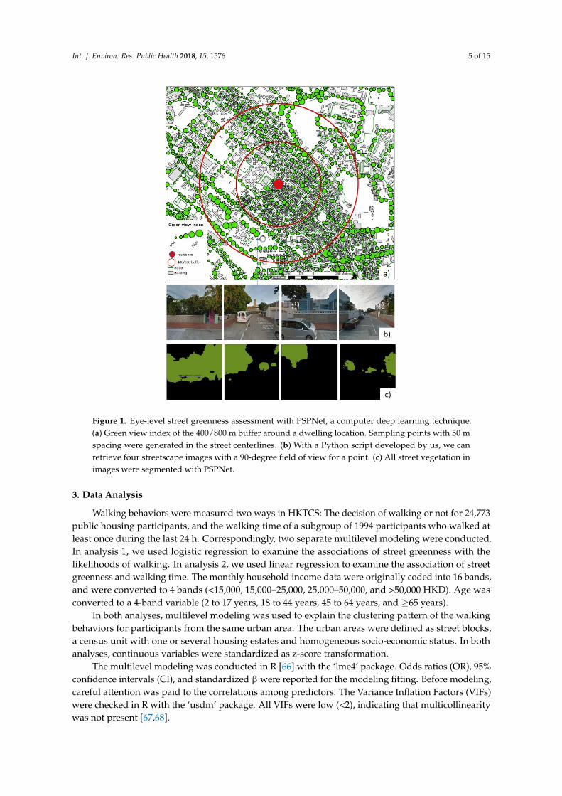
Sampling points were generated in the street centerlines with a 50 m spacing in the buffers(Figure 1b). With a Python script we developed, we can retrieve four streetscape images with a90-degree field of view for a point (Figure 1b). We used the PSPNet trained on the cityscape dataset,a repository of 5000 streetscape images from 50 cities with pixel-level annotations [58]. The trainedmodel achieved a remarkable pixel-level accuracy of 93.4% in terms of identifying vegetation on thecityscape dataset [59]. With the PSPNet greenness extraction function in the script (Figure 1c), theamount of greenness for each point can be determined by the green view index—the proportion ofgreenery pixels in four images—as shown in the following equation [27]:

Green view index =∑4

i = 1 Greenery pixelsi

∑4i = 1 Total pixelsi

(1)

Green view index values range between 0.0 and 1.0, with higher values representing higher levelsof eye-level greenness (Figure 1a). The average green view index for all points in a buffer was usedto assess the neighborhood around a dwelling location. To validate the PSPNet greenness extraction,vegetation was manually selected by an expert using Adobe Photoshop for 50 images. The pixelsrepresenting vegetation in each image was selected using the magic wand tool and adjusted with thelasso tool in Photoshop CS6 (Adobe, San Jose, CA, USA). The selected pixels were then counted inPhotoshop and green view index was calculated again for expert judgement. The amount of streetgreenness extracted by PSPNet and expert judgement were strongly correlated, r(48) = 0.91; p < 0.01.Our validation demonstrated the reliability of GSV greenness extraction.

2.3. Covariates

Other built environment characteristics were also included in this study because of their potentialinfluences on walking behaviors. Street intersection density [60–62], land-use mix [63], populationdensity [60], number of shops, distance to the closest Mass Transit Rail (MTR) station, and numberof bus stops [64,65] were objectively assessed in the buffers of participants’ dwelling locations in GISplatform. The land-use mix was assessed by entropy score to show the degree of land use diversity ofthree types: Commercial, office, and residential [63]. The personal information—including age, genderand household income—were extracted from the HKTCS survey and included in the study.

Int. J. Environ. Res. Public Health 2018, 15, 1576 5 of 15Int. J. Environ. Res. Public Health 2018, 15, x FOR PEER REVIEW    5 of 14 

 

Figure 1. Eye‐level street greenness assessment with PSPNet, a computer deep learning technique. (a) 

Green view  index of the 400/800 m buffer around a dwelling  location. Sampling points with 50 m 

spacing were generated in the street centerlines. (b) With a Python script developed by us, we can 

retrieve four streetscape images with a 90‐degree field of view for a point. (c) All street vegetation in 

images were segmented with PSPNet. 

3. Data Analysis 

Walking behaviors were measured  two ways  in HKTCS: The decision of walking or not  for 

24,773 public housing participants, and  the walking  time of a subgroup of 1994 participants who 

walked at least once during the last 24 h. Correspondingly, two separate multilevel modeling were 

conducted. In analysis 1, we used logistic regression to examine the associations of street greenness 

with the likelihoods of walking. In analysis 2, we used linear regression to examine the association of 

street greenness and walking time. The monthly household income data were originally coded into 

16 bands, and were converted to 4 bands (<15,000, 15,000–25,000, 25,000–50,000, and >50,000 HKD). 

Age was converted to a 4‐band variable (2 to 17 years, 18 to 44 years, 45 to 64 years, and ≥65 years). 

In both analyses, multilevel modeling was used to explain the clustering pattern of the walking 

behaviors for participants from the same urban area. The urban areas were defined as street blocks, 

a census unit with one or several housing estates and homogeneous socio‐economic status. In both 

analyses, continuous variables were standardized as z‐score transformation. 

The multilevel modeling was conducted  in R [66] with the  ‘lme4’ package. Odds ratios (OR), 

95%  confidence  intervals  (CI), and  standardized  β were  reported  for  the modeling  fitting. Before 

modeling, careful attention was paid  to  the correlations among predictors. The Variance  Inflation 

Factors (VIFs) were checked in R with the ‘usdm’ package. All VIFs were low (<2), indicating that 

multicollinearity was not present [67,68]. 

Figure 1. Eye-level street greenness assessment with PSPNet, a computer deep learning technique.(a) Green view index of the 400/800 m buffer around a dwelling location. Sampling points with 50 mspacing were generated in the street centerlines. (b) With a Python script developed by us, we canretrieve four streetscape images with a 90-degree field of view for a point. (c) All street vegetation inimages were segmented with PSPNet.

3. Data Analysis

Walking behaviors were measured two ways in HKTCS: The decision of walking or not for 24,773public housing participants, and the walking time of a subgroup of 1994 participants who walked atleast once during the last 24 h. Correspondingly, two separate multilevel modeling were conducted.In analysis 1, we used logistic regression to examine the associations of street greenness with thelikelihoods of walking. In analysis 2, we used linear regression to examine the association of streetgreenness and walking time. The monthly household income data were originally coded into 16 bands,and were converted to 4 bands (<15,000, 15,000–25,000, 25,000–50,000, and >50,000 HKD). Age wasconverted to a 4-band variable (2 to 17 years, 18 to 44 years, 45 to 64 years, and ≥65 years).

In both analyses, multilevel modeling was used to explain the clustering pattern of the walkingbehaviors for participants from the same urban area. The urban areas were defined as street blocks,a census unit with one or several housing estates and homogeneous socio-economic status. In bothanalyses, continuous variables were standardized as z-score transformation.

The multilevel modeling was conducted in R [66] with the ‘lme4’ package. Odds ratios (OR), 95%confidence intervals (CI), and standardized β were reported for the modeling fitting. Before modeling,careful attention was paid to the correlations among predictors. The Variance Inflation Factors (VIFs)were checked in R with the ‘usdm’ package. All VIFs were low (<2), indicating that multicollinearitywas not present [67,68].

Int. J. Environ. Res. Public Health 2018, 15, 1576 6 of 15

4. Results

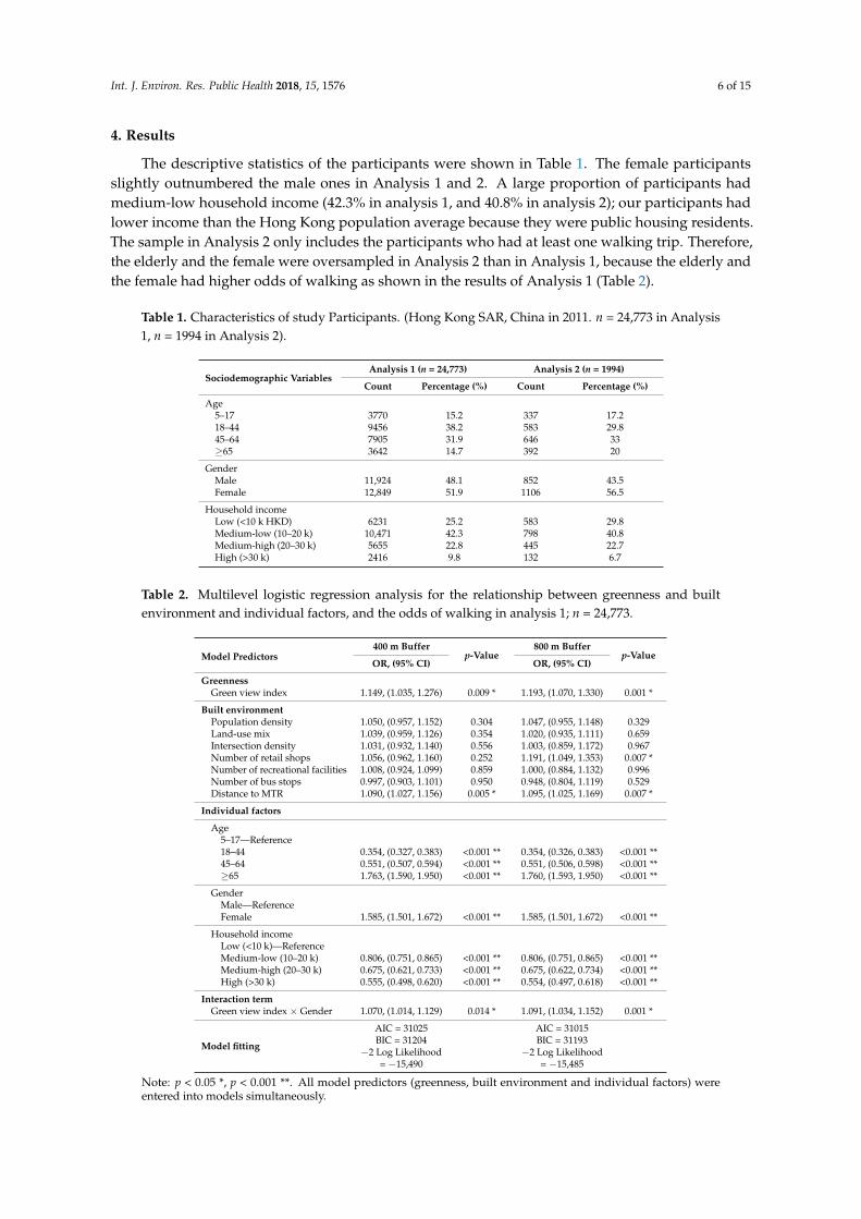
The descriptive statistics of the participants were shown in Table 1. The female participantsslightly outnumbered the male ones in Analysis 1 and 2. A large proportion of participants hadmedium-low household income (42.3% in analysis 1, and 40.8% in analysis 2); our participants hadlower income than the Hong Kong population average because they were public housing residents.The sample in Analysis 2 only includes the participants who had at least one walking trip. Therefore,the elderly and the female were oversampled in Analysis 2 than in Analysis 1, because the elderly andthe female had higher odds of walking as shown in the results of Analysis 1 (Table 2).

Table 1. Characteristics of study Participants. (Hong Kong SAR, China in 2011. n = 24,773 in Analysis1, n = 1994 in Analysis 2).

Sociodemographic VariablesAnalysis 1 (n = 24,773) Analysis 2 (n = 1994)

Count Percentage (%) Count Percentage (%)

Age5–17 3770 15.2 337 17.218–44 9456 38.2 583 29.845–64 7905 31.9 646 33≥65 3642 14.7 392 20

GenderMale 11,924 48.1 852 43.5Female 12,849 51.9 1106 56.5

Household incomeLow (<10 k HKD) 6231 25.2 583 29.8Medium-low (10–20 k) 10,471 42.3 798 40.8Medium-high (20–30 k) 5655 22.8 445 22.7High (>30 k) 2416 9.8 132 6.7

Table 2. Multilevel logistic regression analysis for the relationship between greenness and builtenvironment and individual factors, and the odds of walking in analysis 1; n = 24,773.

Model Predictors400 m Buffer

p-Value800 m Buffer

p-ValueOR, (95% CI) OR, (95% CI)

GreennessGreen view index 1.149, (1.035, 1.276) 0.009 * 1.193, (1.070, 1.330) 0.001 *

Built environmentPopulation density 1.050, (0.957, 1.152) 0.304 1.047, (0.955, 1.148) 0.329Land-use mix 1.039, (0.959, 1.126) 0.354 1.020, (0.935, 1.111) 0.659Intersection density 1.031, (0.932, 1.140) 0.556 1.003, (0.859, 1.172) 0.967Number of retail shops 1.056, (0.962, 1.160) 0.252 1.191, (1.049, 1.353) 0.007 *Number of recreational facilities 1.008, (0.924, 1.099) 0.859 1.000, (0.884, 1.132) 0.996Number of bus stops 0.997, (0.903, 1.101) 0.950 0.948, (0.804, 1.119) 0.529Distance to MTR 1.090, (1.027, 1.156) 0.005 * 1.095, (1.025, 1.169) 0.007 *

Individual factors

Age5–17—Reference18–44 0.354, (0.327, 0.383) <0.001 ** 0.354, (0.326, 0.383) <0.001 **45–64 0.551, (0.507, 0.594) <0.001 ** 0.551, (0.506, 0.598) <0.001 **≥65 1.763, (1.590, 1.950) <0.001 ** 1.760, (1.593, 1.950) <0.001 **

GenderMale—ReferenceFemale 1.585, (1.501, 1.672) <0.001 ** 1.585, (1.501, 1.672) <0.001 **

Household incomeLow (<10 k)—ReferenceMedium-low (10–20 k) 0.806, (0.751, 0.865) <0.001 ** 0.806, (0.751, 0.865) <0.001 **Medium-high (20–30 k) 0.675, (0.621, 0.733) <0.001 ** 0.675, (0.622, 0.734) <0.001 **High (>30 k) 0.555, (0.498, 0.620) <0.001 ** 0.554, (0.497, 0.618) <0.001 **

Interaction termGreen view index × Gender 1.070, (1.014, 1.129) 0.014 * 1.091, (1.034, 1.152) 0.001 *

Model fitting

AIC = 31025BIC = 31204

−2 Log Likelihood= −15,490

AIC = 31015BIC = 31193

−2 Log Likelihood= −15,485

Note: p < 0.05 *, p < 0.001 **. All model predictors (greenness, built environment and individual factors) wereentered into models simultaneously.

Int. J. Environ. Res. Public Health 2018, 15, 1576 7 of 15

The logistic regression results of analysis 1 were shown in Table 2. Interclass correlation coefficient(ICC) for the null model predicting the odds of walking and total walking time was 7.9% and 16.0%respectively, indicating the respective proportion of total outcome variation that is attributed todifferences between street block.

The green view index was related to higher odds of walking in both buffers after adjustingfor covariates (OR (95% CI): 1.149 (1.035, 1.276) in 400 m buffer, 1.193 (1.070, 1.330) in 800 buffer).One standard deviation increase of the green view index increases the likelihood of walking by 14.9%and 19.3% in the 400 m and the 800 m buffers respectively.

Among other built environment factors, distance to MTR station was related to higher oddsof walking in both buffers. Number of shops was positively related to higher odds of walking inthe 800 m buffer, but not in the 400 m buffer. The associations of remaining built environmentfactors were insignificant. Among individual factors, female participants had higher odds of walkingcompared with their male counterparts. Participants in the medium-low, medium-high and highincome group had lower odds of walking compared with those in the low income group. The resultindicates that household income was negatively related with the walking decision. Age has a morecomplex relationship with the odds of walking. Adults (18–44, 45–65 years) had lower odds of walkingand older adults (≥65 years) have higher odds, compared with children (5–17 years). The femaleparticipants had higher odds, compared with the male participants. The interaction term of the greenview index*gender was significant in both buffers, indicating that there is a significant difference bygender in the association of the green view index and the odds of walking. Post-hoc analysis revealedthat the association was stronger for females (1.176 (1.063, 1.301), p = 0.002 in 400 m, 1.235 (1.108, 1.378),p < 0.001 in 800 m) than for males (1.127 (1.002, 1.268), p = 0.046 in 400 m, 1.181 (1.048, 1.331), p = 0.006in 800 m).

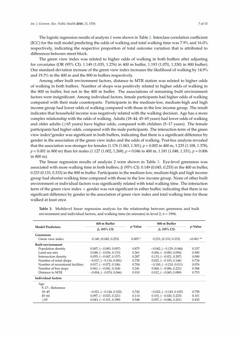
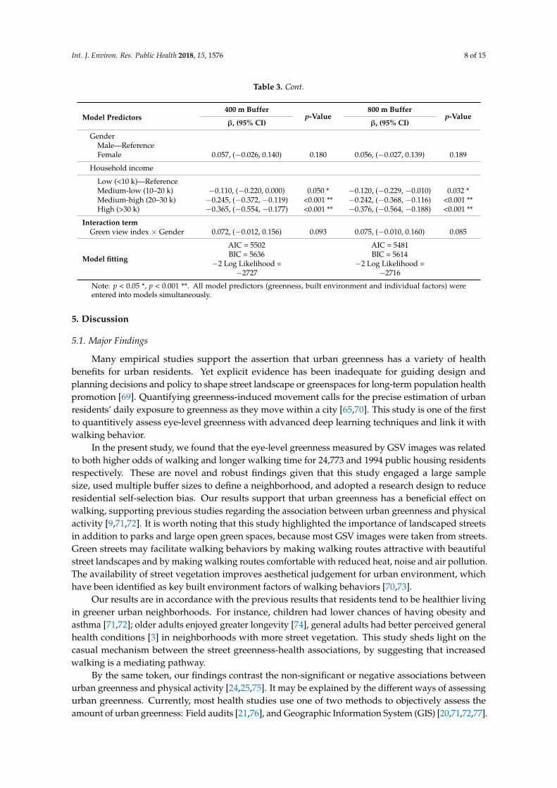
The linear regression results of analysis 2 were shown in Table 3. Eye-level greenness wasassociated with more walking time in both buffers; β (95% CI): 0.149 (0.045, 0.253) in the 400 m buffer,0.233 (0.133, 0.333) in the 800 m buffer. Participants in the medium-low, medium-high and high incomegroup had shorter walking time compared with those in the low income group. None of other builtenvironment or individual factors was significantly related with total walking time. The interactionterm of the green view index × gender was not significant in either buffer, indicating that there is nosignificant difference by gender in the association of green view index and total walking time for thosewalked at least once.

Table 3. Multilevel linear regression analysis for the relationship between greenness and builtenvironment and individual factors, and walking time (in minutes) in level 2; n = 1994.

Model Predictors400 m Buffer

p-Value800 m Buffer

p-Valueβ, (95% CI) β, (95% CI)

GreennessGreen view index 0.149, (0.045, 0.253) 0.005 * 0.233, (0.133, 0.333) <0.001 **

Built environmentPopulation density 0.007, (−0.083, 0.097) 0.875 −0.042, (−0.129, 0.044) 0.337Land-use mix 0.048, (−0.036, 0.133) 0.261 0.006, (−0.083, 0.094) 0.900Intersection density 0.055, (−0.047, 0.157) 0.287 0.133, (−0.021, 0.287) 0.090Number of retail shops −0.017, (−0.116, 0.081) 0.730 0.022, (−0.103, 0.146) 0.734Number of recreational facilities 0.017, (−0.072, 0.106) 0.704 −0.100, (−0.210, 0.011) 0.076Number of bus stops 0.061, (−0.041, 0.164) 0.241 0.068, (−0.086, 0.221) 0.384Distance to MTR −0.004, (−0.074, 0.066) 0.910 0.012, (−0.065, 0.089) 0.753

Individual factors

Age5–17—Reference18–45 −0.021, (−0.144, 0.102) 0.742 −0.022, (−0.143, 0.105) 0.75845–64 0.097, (−0.023, 0.221) 0.114 0.101, (−0.020, 0.223) 0.101≥65 0.043, (−0.101, 0.189) 0.548 0.057, (−0.086, 0.201) 0.430

Int. J. Environ. Res. Public Health 2018, 15, 1576 8 of 15

Table 3. Cont.

Model Predictors400 m Buffer

p-Value800 m Buffer

p-Valueβ, (95% CI) β, (95% CI)

GenderMale—ReferenceFemale 0.057, (−0.026, 0.140) 0.180 0.056, (−0.027, 0.139) 0.189

Household income

Low (<10 k)—ReferenceMedium-low (10–20 k) −0.110, (−0.220, 0.000) 0.050 * −0.120, (−0.229, −0.010) 0.032 *Medium-high (20–30 k) −0.245, (−0.372, −0.119) <0.001 ** −0.242, (−0.368, −0.116) <0.001 **High (>30 k) −0.365, (−0.554, −0.177) <0.001 ** −0.376, (−0.564, −0.188) <0.001 **

Interaction termGreen view index × Gender 0.072, (−0.012, 0.156) 0.093 0.075, (−0.010, 0.160) 0.085

Model fitting

AIC = 5502BIC = 5636

−2 Log Likelihood =−2727

AIC = 5481BIC = 5614

−2 Log Likelihood =−2716

Note: p < 0.05 *, p < 0.001 **. All model predictors (greenness, built environment and individual factors) wereentered into models simultaneously.

5. Discussion

5.1. Major Findings

Many empirical studies support the assertion that urban greenness has a variety of healthbenefits for urban residents. Yet explicit evidence has been inadequate for guiding design andplanning decisions and policy to shape street landscape or greenspaces for long-term population healthpromotion [69]. Quantifying greenness-induced movement calls for the precise estimation of urbanresidents’ daily exposure to greenness as they move within a city [65,70]. This study is one of the firstto quantitively assess eye-level greenness with advanced deep learning techniques and link it withwalking behavior.

In the present study, we found that the eye-level greenness measured by GSV images was relatedto both higher odds of walking and longer walking time for 24,773 and 1994 public housing residentsrespectively. These are novel and robust findings given that this study engaged a large samplesize, used multiple buffer sizes to define a neighborhood, and adopted a research design to reduceresidential self-selection bias. Our results support that urban greenness has a beneficial effect onwalking, supporting previous studies regarding the association between urban greenness and physicalactivity [9,71,72]. It is worth noting that this study highlighted the importance of landscaped streetsin addition to parks and large open green spaces, because most GSV images were taken from streets.Green streets may facilitate walking behaviors by making walking routes attractive with beautifulstreet landscapes and by making walking routes comfortable with reduced heat, noise and air pollution.The availability of street vegetation improves aesthetical judgement for urban environment, whichhave been identified as key built environment factors of walking behaviors [70,73].

Our results are in accordance with the previous results that residents tend to be healthier livingin greener urban neighborhoods. For instance, children had lower chances of having obesity andasthma [71,72]; older adults enjoyed greater longevity [74], general adults had better perceived generalhealth conditions [3] in neighborhoods with more street vegetation. This study sheds light on thecasual mechanism between the street greenness-health associations, by suggesting that increasedwalking is a mediating pathway.

By the same token, our findings contrast the non-significant or negative associations betweenurban greenness and physical activity [24,25,75]. It may be explained by the different ways of assessingurban greenness. Currently, most health studies use one of two methods to objectively assess theamount of urban greenness: Field audits [21,76], and Geographic Information System (GIS) [20,71,72,77].

Int. J. Environ. Res. Public Health 2018, 15, 1576 9 of 15

Field audits are relatively time-consuming and inefficient because the observers need to physicallyvisit all sites. GIS is objective and efficient; yet some street vegetation data, such as shrubs or lawns,were often not collected in GIS. In addition, GIS-based methods generally measure the availability ofstreet greenness from an overhead view, which may significantly differ from the resident’s exposureto those greenness at eye level, especially in locations with dense greenness [26,27]. Hence, the GSVmethod more precisely estimates the resident’s exposure to vegetation in an urban neighborhoodthan other methods. Subjective greenness but not NDVI—an index of greenness based on remotesensing imagery in GIS—was positively related to walking behaviors of 529 participants in Seattle,Washington [25], suggesting residents’ daily exposure to and perception of urban greenness may notbe totally captured by GIS. Therefore, using GSV to quantitively assess eye-level greenness may be anefficient and innovative way to measure the people’s exposure to urban greenness.

It is worth noting that our participants are mostly low-income individuals because this studyfocuses on public housing residents. Household income is demonstrated to be negatively related tothe odds of walking and total walking time; i.e., the poorer participants walk more than the wealthierparticipants (Tables 2 and 3). The results also show that the distance to MTR station was positivelyassociated to the likelihood of walking in both buffers (Table 2). Taking together, these results indicatethat the public transportation system has a greater influence on the poorer individuals than affluentones because poorer people often have no alternative transportation options.

Our results also show that the objectively measured 3D’s of the built environments (populationdensity, land use mix, street intersection density) [73,78–80], were not related to decision of walking orwalking time. Some recent studies from other high-density cities in South America and Asia have alsodemonstrated non-significant or contrary findings [54,81–85], compared with those reported in Westerncountries, especially the United States and Australia [73,78]. It suggests more complex relationshipsbetween the three D’s approach and walking or physical activity, which may be moderated by localbuilt environment and social contexts.

This study also reveals that some individual factors were significantly associated with walkingbehavior. Female participants had higher odds of walking than male participants. The association ofthe green view index and the odds of walking was also stronger for female participants than for maleparticipants. For those who walked at least once during the reference 24 h, gender is not associatedwith total walking time, and there is no significant difference by gender in the association of greenview index and total walking time. Among all age groups, older adults (≥65 years) have the highestodds of walking, followed by children (5–17 years), then adults (18–44, 45–65 years). Older Chineseadults may pay more attention to their personal health for cultural reasons. Household income wasnegatively associated with both the odds of walking and total walking time. Family member ofwealthier household may rely less on the public transportation system, therefore walking less.

The evidence from this study will help government agency develop targeted interventionsin the form of urban planning to promote walking and the general health of residents in HongKong. First, urban planners should consider the location and visibility of urban greenness tomake it effectively exposed to residents. Second, they should also pay close attention to the needsand travel behaviors of poor residents when making design decisions about public transportationinfrastructure (e.g., availability and proximity of MTR stations) because those residents heavily rely onthe public transportation system. Third, contrary to the suggestions for low-density Western cities,increasing urban density, street connectivity or land-use mix may be ineffective to promote walking inhigh-density cities, such as Hong Kong.

5.2. Strength and Limitation

The availability of the GSV dataset, coupled with recent advance in deep learning techniques,provides a unique opportunity to estimate resident’s daily exposure to urban greenness, which inturn sheds lights on the understanding of urban greenness’s impact on physical activity and healthoutcomes. Such advances can help us develop critical evidence for urban planner and policymakers

Int. J. Environ. Res. Public Health 2018, 15, 1576 10 of 15

to make informed decisions about how to design or reshape urban greenness to improve urbanresidents’ wellbeing. Additionally, this study exploited a citywide public housing scheme to reduceself-selection bias, identified as the primary limitation in built environment-health research [28–30].Hence, positive relationships between urban greenness and walking behaviors observed in this studycan be largely attributed to the effect of the environment on physical activity, rather than residentialchoice. Furthermore, the walking data were extracted from a population-level survey; the largesampling size warranted the reliability of our findings.

The study also has several limitations. Though this study reduced residential self-selection bias,we still cannot make any causal inference because of the cross-sectional research design adopted inthis study. Longitudinal studies collecting data over multiple time points are warranted to addressthis issue. The factors of greenery exposure and MTR proximity may be correlated. The areas close toMTR stations often feature higher urban density and lower green view index than the areas far awayfrom MTR stations. It is plausible that a longer walk from or to the MTR station is more likely to resultin greater greenery exposure. Yet, walking routes were not reported by our participants, thereforewe cannot test this assumption. The walking data were self-reported and were thus subject to recallbias. Participants may underreport short walking trips, especially for those living in dense urbanenvironment. The walking and other physical activity behaviors can be objectively collected in futurestudies, such as accelerometers and GPS devices. The neighborhoods boundaries were defined usingcircular buffers rather than street network buffers of participants’ dwelling location, because someinformation of pedestrian infrastructure was unavailable yet, such as footbridges, elevated walkways,or corridors passing through buildings, which are common in the dense urban environment in HongKong. Further studies with detailed data of pedestrian infrastructure may consider using networkbuffers instead. Safety is also one of important factors that is positively associated with walking [73,86].Yet safety-related data, such as traffic incidents or crime rates were currently unavailable. Furtherstudies may incorporate safety-related data in the analysis. Some limitations stem from the GSVservice. Some cities and districts are not covered by GSV. Thus the streetscape images were notaccessible for those areas [35]. GSV images were often taken by cameras installed on top of vehiclesmoving along streets, hence those images may slightly differ from what pedestrians see while walkingalong sidewalks.

6. Conclusions

This study demonstrates that eye-level greenness is positively associated with the odds of walkingand walking time for public housing residents in Hong Kong. Eye-level street greenness assessed byGSV, in conjunction with deep learning techniques, can accurately and effectively estimate people’sexposure to urban greenness, compared with existing methods. Therefore, it can contribute tomethodological development of health studies. The findings of this study also have some implicitplanning applications. Governments and urban planners should consider not only the provision ofurban greenness in terms of general density or size, but also the visibility of the greenness from apedestrian’s perspective while moving through a city.

Funding: The work described in this paper was fully supported by grants from the Research Grants Councilof the Hong Kong Special Administrative Region, China (Project Nos. CityU11612615 & CityU11666716) andthe National Natural Science Foundation of China (Project Nos. 51578474 & 51778552). The APC was fundedby CityU11612615.

Conflicts of Interest: The author declares no conflict of interest. The funding sponsors had no role in the designof the study; in the collection, analyses, or interpretation of data; in the writing of the manuscript, and in thedecision to publish the results.

References

1. Ulrich, R.S. Biophilia, biophobia, and natural landscapes. In The Biophilia Hypothesis; Kellert, S.R.,Wilson, E.O., Eds.; Island Press: Washington, DC, USA, 1993; pp. 73–137.

Int. J. Environ. Res. Public Health 2018, 15, 1576 11 of 15

2. Coon, J.T.; Boddy, K.; Stein, K.; Whear, R.; Barton, J.; Depledge, M.H. Does Participating in Physical Activityin Outdoor Natural Environments Have a Greater Effect on Physical and Mental Wellbeing than PhysicalActivity Indoors? A Systematic Review. Environ. Sci. Technol. 2011, 45, 1761–1772. [CrossRef] [PubMed]

3. Ulrich, R.S. View through a window may influence recovery from surgery. Science 1984, 224, 420–421.[CrossRef] [PubMed]

4. Pretty, J.; Peacock, J.; Hine, R.; Sellens, M.; South, N.; Griffin, M. Green exercise in the UK countryside: Effectson health and psychological well-being, and implications for policy and planning. J. Environ. Plan. Manag.2007, 50, 211–231. [CrossRef]

5. Sarkar, C. Residential greenness and adiposity: Findings from the UK Biobank. Environ. Int. 2017, 106, 1–10.[CrossRef] [PubMed]

6. Mitchell, R.; Popham, F. Effect of exposure to natural environment on health inequalities: An observationalpopulation study. Lancet 2008, 372, 1655–1660. [CrossRef]

7. Stigsdotter, U.K.; Ekholm, O.; Schipperijn, J.; Toftager, M.; Kamper-Jorgensen, F.; Randrup, T.B. Healthpromoting outdoor environments—Associations between green space, and health, health-related quality oflife and stress based on a Danish national representative survey. Scand. J. Public Health 2010, 38, 411–417.[CrossRef] [PubMed]

8. Markevych, I.; Schoierer, J.; Hartig, T.; Chudnovsky, A.; Hystad, P.; Dzhambov, A.M.; de Vries, S.;Triguero-Mas, M.; Brauer, M.; Nieuwenhuijsen, M.J.; et al. Exploring pathways linking greenspace tohealth: Theoretical and methodological guidance. Environ. Res. 2017, 158, 301–317. [CrossRef] [PubMed]

9. Hartig, T.; Mitchell, R.; de Vries, S.; Frumkin, H. Nature and Health. Annu. Rev. Public Health 2014, 35,207–228. [CrossRef] [PubMed]

10. Pretty, J.; Hine, R.; Peacock, J. Green exercise: The benefits of activities in green places. Biologist 2006, 53,143–148.

11. Pretty, J.; Peacock, J.; Sellens, M.; Griffin, M. The mental and physical health outcomes of green exercise. Int.J. Environ. Health Res. 2005, 15, 319–337. [CrossRef] [PubMed]

12. van den Berg, A.E.; Hartig, T.; Staats, H. Preference for nature in urbanized societies: Stress, restoration, andthe pursuit of sustainability. J. Soc. Issues 2007, 63, 79–96. [CrossRef]

13. Barton, J.; Pretty, J. What is the best dose of nature and green exercise for improving mental health—Amulti-study analysis. Environ. Sci. Technol. 2010, 44, 3947–3955. [CrossRef] [PubMed]

14. Kaczynski, A.T.; Henderson, K.A. Environmental correlates of physical activity: A review of evidence aboutparks and recreation. Leis. Sci. 2007, 29, 315–354. [CrossRef]

15. Coombes, E.; Jones, A.P.; Hillsdon, M. The relationship of physical activity and overweight to objectivelymeasured green space accessibility and use. Soc. Sci. Med. 2010, 70, 816–822. [CrossRef] [PubMed]

16. Floyd, M.F.; Spengler, J.O.; Maddock, J.E.; Gobster, P.H.; Suau, L. Environmental and social correlates ofphysical activity in neighborhood parks: An observational study in Tampa and Chicago. Leis. Sci. 2008, 30,360–375. [CrossRef]

17. Giles-Corti, B.; Broomhall, M.H.; Knuiman, M.; Collins, C.; Douglas, K.; Ng, K.; Lange, A.; Donovan, R.J.Increasing walking—How important is distance to, attractiveness, and size of public open space? Am. J.Prev. Med. 2005, 28, 169–176. [CrossRef] [PubMed]

18. Kaczynski, A.T.; Potwarka, L.R.; Smale, B.J.A.; Havitz, M.E. Association of Parkland Proximity withNeighborhood and Park-based Physical Activity: Variations by Gender and Age. Leis. Sci. 2009, 31,174–191. [CrossRef]

19. Koohsari, M.J.; Karakiewicz, J.A.; Kaczynski, A.T. Public Open Space and Walking: The Role of Proximity,Perceptual Qualities of the Surrounding Built Environment, and Street Configuration. Environ. Behav. 2013,45, 706–736. [CrossRef]

20. Sarkar, C.; Webster, C.; Pryor, M.; Tang, D.; Melbourne, S.; Zhang, X.H.; Liu, J.Z. Exploring associationsbetween urban green, street design and walking: Results from the Greater London boroughs. Landsc. UrbanPlan. 2015, 143, 112–125. [CrossRef]

21. Van Dillen, S.M.E.; de Vries, S.; Groenewegen, P.P.; Spreeuwenberg, P. Greenspace in urban neighbourhoodsand residents’ health: Adding quality to quantity. J. Epidemiol. Community Health 2012, 66, e8. [CrossRef][PubMed]

22. Xiao, Y.; Lu, Y.; Guo, Y.; Yuan, Y. Estimating the willingness to pay for green space services in Shanghai:Implications for social equity in urban China. Urban For. Urban Green. 2017, 26, 95–103. [CrossRef]

Int. J. Environ. Res. Public Health 2018, 15, 1576 12 of 15

23. Lu, Y.; Sarkar, C.; Ye, Y.; Xiao, Y. Using the Online Walking Journal to explore the relationship betweencampus environment and walking behaviour. J. Transp. Health 2017, 5, 123–132. [CrossRef]

24. Duncan, M.; Mummery, K. Psychosocial and environmental factors associated with physical activity amongcity dwellers in regional Queensland. Prev. Med. 2005, 40, 363–372. [CrossRef] [PubMed]

25. Jenna, H.T.; Thomas, M.U.; Belen, R. Using Objective and Subjective Measures of Neighborhood Greennessand Accessible Destinations for Understanding Walking Trips and BMI in Seattle, Washington. Am. J. HealthPromot. 2007, 21, 371–379.

26. Jiang, B.; Deal, B.; Pan, H.Z.; Larsen, L.; Hsieh, C.H.; Chang, C.Y.; Sullivan, W.C. Remotely-sensed imageryvs. eye-level photography: Evaluating associations among measurements of tree cover density. Landsc.Urban Plan. 2017, 157, 270–281. [CrossRef]

27. Li, X.J.; Zhang, C.R.; Li, W.D.; Ricard, R.; Meng, Q.Y.; Zhang, W.X. Assessing street-level urban greeneryusing Google Street View and a modified green view index. Urban For. Urban Green. 2015, 14, 675–685.[CrossRef]

28. Boone-Heinonen, J.; Gordon-Larsen, P.; Guilkey, D.K.; Jacobs, D.R.; Popkin, B.M. Environment and physicalactivity dynamics: The role of residential self-selection. Psychol. Sport Exerc. 2011, 12, 54–60. [CrossRef][PubMed]

29. Frank, L.D.; Saelens, B.E.; Powell, K.E.; Chapman, J.E. Stepping towards causation: Do built environments orneighborhood and travel preferences explain physical activity, driving, and obesity? Soc. Sci. Med. 2007, 65,1898–1914. [CrossRef] [PubMed]

30. Diez Roux, A.V. Estimating neighborhood health effects: The challenges of causal inference in a complexworld. Soc. Sci. Med. 2004, 58, 1953–1960. [CrossRef]

31. Bagley, M.N.; Mokhtarian, P.L. The impact of residential neighborhood type on travel behavior: A structuralequations modeling approach. Ann. Reg. Sci. 2002, 36, 279–297. [CrossRef]

32. Handy, S.L.; Cao, X.; Mokhtarian, P.L. Self-selection in the relationship between the built environment andwalking: Empirical evidence from Northern California. J. Am. Plan. Assoc. 2006, 72, 55–74. [CrossRef]

33. Cao, X.; Mokhtarian, P.L.; Handy, S.L. Examining the impacts of residential self-selection on travel behaviour:A focus on empirical findings. Transp. Rev. 2009, 29, 359–395. [CrossRef]

34. Mokhtarian, P.L.; Cao, X. Examining the impacts of residential self-selection on travel behavior: A focus onmethodologies. Transp. Res. Part B Methodol. 2008, 42, 204–228. [CrossRef]

35. Google Inc. Understand Google Street View 2016. Available online: https://www.google.com/streetview/understand/ (accessed on 1 February 2017).

36. Charreire, H.; Mackenbach, J.D.; Ouasti, M.; Lakerveld, J.; Compernolle, S.; Ben-Rebah, M.; Mckee, M.;Brug, J.; Rutter, H.; Oppert, J.M. Using remote sensing to define environmental characteristics related tophysical activity and dietary behaviours: A systematic review (the SPOTLIGHT project). Health Place 2014,25, 1–9. [CrossRef] [PubMed]

37. Rundle, A.G.; Bader, M.D.M.; Richards, C.A.; Neckerman, K.M.; Teitler, J.O. Using Google Street View toAudit Neighborhood Environments. Am. J. Prev. Med. 2011, 40, 94–100. [CrossRef] [PubMed]

38. Edwards, N.; Hooper, P.; Trapp, G.S.A.; Bull, F.; Boruff, B.; Giles-Corti, B. Development of a Public OpenSpace Desktop Auditing Tool (POSDAT): A remote sensing approach. Appl. Geogr. 2013, 38, 22–30. [CrossRef]

39. Liang, J.; Gong, J.; Sun, J.; Zhou, J.; Li, W.; Li, Y.; Liu, J.; Shen, S. Automatic sky view factor estimation fromstreet view photographs—A big data approach. Remote Sens. 2017, 9, 411. [CrossRef]

40. Lu, Y.; Sarkar, C.; Xiao, Y. The effect of street-level greenery on walking behavior: Evidence from Hong Kong.Soc. Sci. Med. 2018, 208, 41–49. [CrossRef] [PubMed]

41. Poursaeed, O.; Matera, T.; Belongie, S. Vision-based real estate price estimation. Mach. Vis. Appl. 2018, 29,667–676. [CrossRef]

42. Wegner, J.D.; Branson, S.; Hall, D.; Schindler, K.; Perona, P. Cataloging Public Objects Using Aerial andStreet-Level Images—Urban Trees. In Proceedings of the 2016 IEEE Conference on Computer Vision andPattern Recognition (CVPR), Las Vegas, NV, USA, 27–30 June 2016; pp. 6014–6023. [CrossRef]

43. Garcia-Garcia, A.; Orts, S.; Oprea, S.; Villena-Martinez, V.; Rodriguez, J.G. A Review on Deep LearningTechniques Applied to Semantic Segmentation. Available online: https://arxiv.org/pdf/1704.06857.pdf(accessed on 24 July 2018).

44. Seiferling, I.; Naik, N.; Ratti, C.; Proulx, R. Green streets—Quantifying and mapping urban trees withstreet-level imagery and computer vision. Landsc. Urban Plan. 2017, 165, 93–101. [CrossRef]

Int. J. Environ. Res. Public Health 2018, 15, 1576 13 of 15

45. Zhao, H.; Shi, J.; Qi, X.; Wang, X.; Jia, J. Pyramid scene parsing network. In Proceedings of the 30th IEEEConference on Computer Vision and Pattern Recognition (CVPR), Washington, DC, USA, 30 May–3 June2017; pp. 6230–6239.

46. Hong Kong Housing Authority. Report on Population and Households in Housing Authority Public RentalHousing. 2017. Available online: https://www.housingauthority.gov.hk/en/common/pdf/about-us/publications-and-statistics/PopulationReport.pdf (accessed on 10 February 2017).

47. Housing Authority of Hong Kong. Report on Population and Households in Housing Authority Public RentalHousing; Housing Authority of Hong Kong: Hong Kong, China, 2013.

48. Danaei, G.; Ding, E.L.; Mozaffarian, D.; Taylor, B.; Rehm, J.; Murray, C.J.L.; Ezzati, M. The preventable causesof death in the United States: Comparative risk assessment of dietary, lifestyle, and metabolic risk factors.PLoS Med. 2009, 6, e1000058. [CrossRef] [PubMed]

49. Census & Statistics Department of Hong Kong. Population Estimates. 2016. Available online: http://www.censtatd.gov.hk/hkstat/sub/so150.jsp (accessed on 10 October 2016).

50. Cerin, E.; Nathan, A.; van Cauwenberg, J.; Barnett, D.W.; Barnett, A. The neighbourhood physicalenvironment and active travel in older adults: A systematic review and meta-analysis. Int. J. Behav.Nutr. Phys. Act. 2017, 14. [CrossRef] [PubMed]

51. Bohannon, R.W. Comfortable and maximum walking speed of adults aged 20–79 years: Reference valuesand determinants. Age Ageing 1997, 26, 15–19. [CrossRef] [PubMed]

52. Langlois, M.; Wasfi, R.A.; Ross, N.A.; El-Geneidy, A.M. Can transit-oriented developments help achieve therecommended weekly level of physical activity? J. Transp. Health 2016, 3, 181–190. [CrossRef]

53. Day, K. Built environmental correlates of physical activity in China: A review. Prev. Med. Rep. 2016, 3,303–316. [CrossRef] [PubMed]

54. Salvo, D.; Reis, R.S.; Stein, A.D.; Rivera, J.; Martorell, R.; Pratt, M. Characteristics of the Built Environment inRelation to Objectively Measured Physical Activity Among Mexican Adults, 2011. Prev. Chronic Dis. 2014,11, E147. [CrossRef] [PubMed]

55. McCormack, G.R.; Shiell, A. In search of causality: A systematic review of the relationship between the builtenvironment and physical activity among adults. Int. J. Behav. Nutr. Phys. Act. 2011, 8, 125. [CrossRef][PubMed]

56. Mazumdar, S.; Rushton, G.; Smith, B.J.; Zimmerman, D.L.; Donham, K.J. Geocoding accuracy and therecovery of relationships between environmental exposures and health. Int. J. Health Geogr. 2008, 7, 13.[CrossRef] [PubMed]

57. Swift, A.; Liu, L.; Uber, J. MAUP sensitivity analysis of ecological bias in health studies. GeoJournal 2014, 79,137–153. [CrossRef]

58. Cordts, M.; Omran, M.; Ramos, S.; Rehfeld, T.; Enzweiler, M.; Benenson, R.; Franke, U.; Roth, S.; Schiele, B.The Cityscapes Dataset for Semantic Urban Scene Understanding. In Proceedings of the 2016 IEEEConference on Computer Vision and Pattern Recognition (CVPR), Las Vegas, NV, USA, 27–30 June 2016;pp. 3213–3223. [CrossRef]

59. Zhao, H.; Shi, J.; Qi, X.; Wang, X.; Jia, J. Pyramid Scene Parsing Network. 2017. Available online: https://hszhao.github.io/projects/pspnet/ (accessed on 11 December 2017).

60. Li, F.Z.; Fisher, K.J.; Brownson, R.C.; Bosworth, M. Multilevel modelling of built environment characteristicsrelated to neighbourhood walking activity in older adults. J. Epidemiol. Community Health 2005, 59, 558–564.[CrossRef] [PubMed]

61. Adkins, A.; Dill, J.; Luhr, G.; Neal, M. Unpacking Walkability: Testing the Influence of Urban Design Featureson Perceptions of Walking Environment Attractiveness. J. Urban Des. 2012, 17, 499–510. [CrossRef]

62. Chin, G.K.W.; Van Niel, K.P.; Giles-Corti, B.; Knuiman, M. Accessibility and connectivity in physical activitystudies: The impact of missing pedestrian data. Prev. Med. 2008, 46, 41–45. [CrossRef] [PubMed]

63. Frank, L.D.; Schmid, T.L.; Sallis, J.F.; Chapman, J.; Saelens, B.E. Linking objectively measured physicalactivity with objectively measured urban form: Findings from SMARTRAQ. Am. J. Prev. Med. 2005, 28,117–125. [CrossRef] [PubMed]

64. Hajna, S.; Ross, N.A.; Brazeau, A.-S.; Bélisle, P.; Joseph, L.; Dasgupta, K. Associations between neighbourhoodwalkability and daily steps in adults: A systematic review and meta-analysis. BMC Public Health 2015, 15,1–8. [CrossRef] [PubMed]

Int. J. Environ. Res. Public Health 2018, 15, 1576 14 of 15

65. Lee, I.M.; Shiroma, E.J.; Lobelo, F.; Puska, P.; Blair, S.N.; Katzmarzyk, P.T. Impact of Physical Inactivity on theWorld’s Major Non-Communicable Diseases. Lancet 2012, 380, 219–229. [CrossRef]

66. R Core Team. R: A Language and Environment for Statistical Computing; R Foundation for Statistical Computing:Vienna, Austria, 2014.

67. Mertens, L.; Compernolle, S.; Deforche, B.; Mackenbach, J.D.; Lakerveld, J.; Brug, J.; Roda, C.; Feuillet, T.;Oppert, J.M.; Glonti, K.; et al. Built environmental correlates of cycling for transport across Europe.Health Place 2017, 44, 35–42. [CrossRef] [PubMed]

68. Naimi, B.; Hamm, N.A.S.; Groen, T.A.; Skidmore, A.K.; Toxopeus, A.G. Where is positional uncertainty aproblem for species distribution modelling? Ecography 2014, 37, 191–203. [CrossRef]

69. Lee, A.C.K.; Maheswaran, R. The health benefits of urban green spaces: A review of the evidence. J. PublicHealth 2011, 33, 212–222. [CrossRef] [PubMed]

70. Sallis, J.F.; Floyd, M.F.; Rodríguez, D.A.; Saelens, B.E. Role of Built Environments in Physical Activity, Obesity,and Cardiovascular Disease. Circulation 2012, 125, 729–737. [CrossRef] [PubMed]

71. Lovasi, G.S.; Quinn, J.W.; Neckerman, K.M.; Perzanowski, M.S.; Rundle, A. Children living in areas withmore street trees have lower prevalence of asthma. J. Epidemiol. Community Health 2008, 62, 647–649.[CrossRef] [PubMed]

72. Lovasi, G.S.; Schwartz-Soicher, O.; Quinn, J.W.; Berger, D.K.; Neckerman, K.M.; Jaslow, R.; Lee, K.K.;Rundle, A. Neighborhood safety and green space as predictors of obesity among preschool children fromlow-income families in New York City. Prev. Med. 2013, 57, 189–193. [CrossRef] [PubMed]

73. Saelens, B.E.; Handy, S.L. Built environment correlates of walking: A review. Med. Sci. Sports Exerc. 2008, 40,S550–S566. [CrossRef] [PubMed]

74. Takano, T.; Nakamura, K.; Watanabe, M. Urban residential environments and senior citizens’ longevity inmegacity areas: The importance of walkable green spaces. J. Epidemiol. Community Health 2002, 56, 913–918.[CrossRef] [PubMed]

75. King, W.C.; Belle, S.H.; Brach, J.S.; Simkin-Silverman, L.R.; Soska, T.; Kriska, A.M. Objective measures ofneighborhood environment and physical activity in older women. Am. J. Prevent. Med. 2005, 28, 461–469.[CrossRef] [PubMed]

76. De Vries, S.; van Dillen, S.M.E.; Groenewegen, P.P.; Spreeuwenberg, P. Streetscape greenery and health: Stress,social cohesion and physical activity as mediators. Soc. Sci. Med. 2013, 94, 26–33. [CrossRef] [PubMed]

77. Lovasi, G.S.; Jacobson, J.S.; Quinn, J.W.; Neckerman, K.M.; Ashby-Thompson, M.N.; Rundle, A. Is theenvironment near home and school associated with physical activity and adiposity of urban preschoolchildren? J. Urban Health 2011, 88, 1143–1157. [CrossRef] [PubMed]

78. Grasser, G.; Van Dyck, D.; Titze, S.; Stronegger, W. Objectively measured walkability and active transport andweight-related outcomes in adults: A systematic review. Int. J. Public Health 2013, 58, 615–625. [CrossRef][PubMed]

79. Van Holle, V.; Deforche, B.; Van Cauwenberg, J.; Goubert, L.; Maes, L.; Van de Weghe, N.; De Bourdeaudhuij, I.Relationship between the physical environment and different domains of physical activity in Europeanadults: A systematic review. BMC Public Health 2012, 12. [CrossRef] [PubMed]

80. Ewing, R.; Cervero, R. Travel and the built environment: A meta-analysis. J. Am. Plan. Assoc. 2010, 76,265–294. [CrossRef]

81. Gomez, L.F.; Sarmiento, O.L.; Parra, D.C.; Schmid, T.L.; Pratt, M.; Jacoby, E.; Neiman, A.; Cervero, R.;Mosquera, J.; Rutt, C.; et al. Characteristics of the Built Environment Associated With Leisure-Time PhysicalActivity Among Adults in Bogota, Colombia: A Multilevel Study. J. Phys. Act. Health 2010, 7, S196–S203.[CrossRef] [PubMed]

82. Xu, F.; Li, J.; Liang, Y.; Wang, Z.; Hong, X.; Ware, R.S.; Leslie, E.; Sugiyama, T.; Owen, N. Associationsof residential density with adolescents’ physical activity in a rapidly urbanizing area of mainland China.J. Urban Health Bull. N. Y. Acad. Med. 2010, 87, 44–53. [CrossRef] [PubMed]

83. Su, M.; Tan, Y.-Y.; Liu, Q.-M.; Ren, Y.-J.; Kawachi, I.; Li, L.-M.; Lv, J. Association between perceived urbanbuilt environment attributes and leisure-time physical activity among adults in Hangzhou, China. Prev. Med.2014, 66, 60–64. [CrossRef] [PubMed]

84. Siqueira Reis, R.; Hino, A.A.F.; Ricardo Rech, C.; Kerr, J.; Curi Hallal, P. Walkability and Physical Activity:Findings from Curitiba, Brazil. Am. J. Prev. Med. 2013, 45, 269–275. [CrossRef] [PubMed]

Int. J. Environ. Res. Public Health 2018, 15, 1576 15 of 15

85. Lu, Y.; Xiao, Y.; Ye, Y. Urban density, diversity and design: Is more always better for walking? A study fromHong Kong. Prev. Med. 2017, 103, S99–S103. [CrossRef] [PubMed]

86. Ding, D.; Gebel, K. Built environment, physical activity, and obesity: What have we learned from reviewingthe literature? Health Place 2012, 18, 100–105. [CrossRef] [PubMed]

© 2018 by the author. Licensee MDPI, Basel, Switzerland. This article is an open accessarticle distributed under the terms and conditions of the Creative Commons Attribution(CC BY) license (http://creativecommons.org/licenses/by/4.0/).