
The Artificial Boundary Method for a Nonlinear Interface ... · The ArtificialBoundaryMethod for...
26
Copyright © 2008 Tech Science Press CMES, vol.35, no.3, pp.227-252, 2008 The Artificial Boundary Method for a Nonlinear Interface Problem on Unbounded Domain De-hao Yu 1 and Hong-ying Huang 2 Abstract: In this paper, we apply the artificial boundary method to solve a three- dimensional nonlinear interface problem on an unbounded domain. A spherical or ellipsoidal surface as the artificial boundary is introduced. The exact artificial boundary conditions are derived explicitly in terms of an infinite series and then the well-posedness of the coupled weak formulation in a bounded domain, which is equivalent to the original problem in the unbounded domain, is obtained. The error estimate depends on the mesh size, the term after truncating the infinite series and the location of the artificial boundary. Some numerical examples are presented to demonstrate the effectiveness and accuracy of this method. Keyword: Artificial boundary method, Dirichlet to Neumann mapping, Finite element method, Natural integral operator, Nonlinear interface problem. 1 Introduction In many fields of scientific and engineering computing, the boundary value prob- lems of the partial differential equations on some unbounded domains are often met. The boundlessness of the domains brings the essential difficulties for solving these problems numerically. There are several methods for solving these problems. The artificial boundary method is one of them. It is particularly attractive for exte- rior problems or problems in domains extending to infinity. The artificial boundary method reduces the original problem in an unbounded do- main to an equivalent problem in a bounded domain with some suitable boundary conditions on the artificial boundary. The standard procedure of the method may be simply described as follows. First, one divides the domain into two subregions, a bounded inner region and an unbounded outer region by introducing an auxil- 1 LSEC, ICMSEC, Academy of Mathematics and System Sciences, The Chinese Academy of Sci- ences, Beijing, 100190, China. 2 School of Mathematics, Physics and Information Science, Zhejiang Ocean University, Zhoushan, Zhejiang, 316004, China.
Transcript of The Artificial Boundary Method for a Nonlinear Interface ... · The ArtificialBoundaryMethod for...
Copyright © 2008 Tech Science Press CMES, vol.35, no.3, pp.227-252, 2008
The Artificial Boundary Method for a Nonlinear InterfaceProblem on Unbounded Domain
De-hao Yu1 and Hong-ying Huang2
Abstract: In this paper, we apply the artificial boundary method to solve a three-dimensional nonlinear interface problem on an unbounded domain. A sphericalor ellipsoidal surface as the artificial boundary is introduced. The exact artificialboundary conditions are derived explicitly in terms of an infinite series and thenthe well-posedness of the coupled weak formulation in a bounded domain, whichis equivalent to the original problem in the unbounded domain, is obtained. Theerror estimate depends on the mesh size, the term after truncating the infinite seriesand the location of the artificial boundary. Some numerical examples are presentedto demonstrate the effectiveness and accuracy of this method.
Keyword: Artificial boundary method, Dirichlet to Neumann mapping, Finiteelement method, Natural integral operator, Nonlinear interface problem.
1 Introduction
In many fields of scientific and engineering computing, the boundary value prob-lems of the partial differential equations on some unbounded domains are oftenmet. The boundlessness of the domains brings the essential difficulties for solvingthese problems numerically. There are several methods for solving these problems.The artificial boundary method is one of them. It is particularly attractive for exte-rior problems or problems in domains extending to infinity.
The artificial boundary method reduces the original problem in an unbounded do-main to an equivalent problem in a bounded domain with some suitable boundaryconditions on the artificial boundary. The standard procedure of the method maybe simply described as follows. First, one divides the domain into two subregions,a bounded inner region and an unbounded outer region by introducing an auxil-
1 LSEC, ICMSEC, Academy of Mathematics and System Sciences, The Chinese Academy of Sci-ences, Beijing, 100190, China.
2 School of Mathematics, Physics and Information Science, Zhejiang Ocean University, Zhoushan,Zhejiang, 316004, China.
228 Copyright © 2008 Tech Science Press CMES, vol.35, no.3, pp.227-252, 2008
iary common boundary. Next, the problem is reduced to an equivalent one in thebounded inner region. This reduction will be accomplished by deriving either a lo-cal natural boundary condition or a nonlocal boundary condition, which relates theCauchy data of the solution on the common boundary. Because of the necessity ofderiving this boundary condition on the common boundary, one needs generally toapply boundary integral methods to the unbounded outer region. This reduction toan equivalent problem is by no means a unique process. The first significant resultconcerning the theoretical justification of a coupling procedure of this type seemsdue to Brezzi and Johnson (1979) and Johnson and Nedelec (1980). It is basedon the classical direct boundary integral method. Further theoretical developmentswith respect to various coupling procedures may be found in Wendland (1986),Costabel (1987), Feng (1983), Han (1990), Hsiao and Proter (1986), MacCamyand Marin (1980). Most of these coupling methods are not direct and natural. Adirect and natural coupling of the finite and boundary elements was suggested firstby Feng and Yu (1983), where the imposed boundary condition on the artificialboundary is exact, non-reflective and nonlocal. The method leads to a symmet-ric and coercive bilinear form and then this method is called the natural couplingmethod of FEM and BEM, or the exact artificial boundary method. Because theexact artificial boundary condition is just the Dirichlet to Neumann mapping on theartificial boundary, this method is also called the DtN method [Keller and Givoli(1989), Grote and Keller (1995)].
Yu (2002) has given many kinds of equivalent forms of the natural boundary inte-gral operator, i.e., the exact artificial boundary condition for the two-dimensionalelliptic problems, Stokes equations and linear elastic equations on the circle artifi-cial boundary. Wu and Yu (2000) obtained the exact artificial boundary conditionbased on the elliptic boundary while Wu (1999), Grote and Keller (1995) attainedthe exact artificial boundary one on the spherical boundary. More recently, Huangand Yu (2007) derive the exact artificial boundary one on the spheroidal boundaryand general ellipsoidal boundary. The exact artificial boundary condition is gener-ally expressed explicitly in terms of an infinite series. However, in the numericalcomputation, the infinite series need to be truncated and then this will result inthe truncation error. The error estimate of the numerical approximation solutionwhich has first been given by Yu (1985) showed how the error depend on the meshsize, the position of the artificial boundary and the term after truncating the infi-nite series. The artificial boundary method, originally designed for treating linearproblems [Yu (2002)], works equally well for the case of the evolution equationby Du and Yu (2000, 2001), the electromagnetic problems by Liu (2007), an ade-quate combination of linear and nonlinear partial differential equations by Hu andYu (2001).
The Artificial Boundary Method for a Nonlinear Interface Problem 229
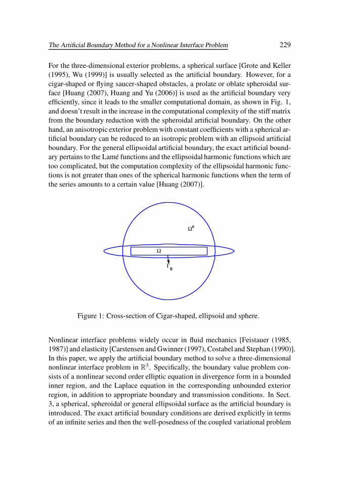
For the three-dimensional exterior problems, a spherical surface [Grote and Keller(1995), Wu (1999)] is usually selected as the artificial boundary. However, for acigar-shaped or flying saucer-shaped obstacles, a prolate or oblate spheroidal sur-face [Huang (2007), Huang and Yu (2006)] is used as the artificial boundary veryefficiently, since it leads to the smaller computational domain, as shown in Fig. 1,and doesn’t result in the increase in the computational complexity of the stiff matrixfrom the boundary reduction with the spheroidal artificial boundary. On the otherhand, an anisotropic exterior problem with constant coefficients with a spherical ar-tificial boundary can be reduced to an isotropic problem with an ellipsoid artificialboundary. For the general ellipsoidal artificial boundary, the exact artificial bound-ary pertains to the Lamé functions and the ellipsoidal harmonic functions which aretoo complicated, but the computation complexity of the ellipsoidal harmonic func-tions is not greater than ones of the spherical harmonic functions when the term ofthe series amounts to a certain value [Huang (2007)].
Γ0
Ω
Ωc
Figure 1: Cross-section of Cigar-shaped, ellipsoid and sphere.
Nonlinear interface problems widely occur in fluid mechanics [Feistauer (1985,1987)] and elasticity [Carstensen and Gwinner (1997), Costabel and Stephan (1990)].In this paper, we apply the artificial boundary method to solve a three-dimensionalnonlinear interface problem in R
3. Specifically, the boundary value problem con-sists of a nonlinear second order elliptic equation in divergence form in a boundedinner region, and the Laplace equation in the corresponding unbounded exteriorregion, in addition to appropriate boundary and transmission conditions. In Sect.3, a spherical, spheroidal or general ellipsoidal surface as the artificial boundary isintroduced. The exact artificial boundary conditions are derived explicitly in termsof an infinite series and then the well-posedness of the coupled variational problem
230 Copyright © 2008 Tech Science Press CMES, vol.35, no.3, pp.227-252, 2008
is obtained. In Sect. 4, we give existence and uniqueness of the solution of thediscrete problem and derive asymptotic error estimate. The error estimate showsthe error depends on the mesh size, the term after truncating the infinite series andthe location of the artificial boundary. Some numerical examples are presented inSect. 5 to demonstrate the effectiveness and accuracy of this method. Finally, westate the conclusions in Sect. 6.
2 The problem described
We consider a nonlinear elliptic differential equation in a bounded Lipschitz do-main Ω ⊂ R
3 and a linear elliptic differential equation in Ωc := R3\(Ω∪∂Ω) and
their solutions are connected by conditions on the interface boundary Γ0 = ∂Ω. Forgiven f ∈ L2(Ω),u0 ∈ H1/2(Γ0), t0 ∈ H−1/2(Γ0) , the interface problem reads: findu1 ∈ H1(Ω), u2 ∈ H1
loc(Ωc) such that
−div(p(|∇u1|) ·∇u1)+u1 = f , in Ω, (1)
−Δu2 = 0, in Ωc, (2)
with the transmission conditions
u1 = u2 +u0, p(|∇u1|)∂u1
∂n=
∂u2
∂n+ t0 on Γ0, (3)
and the radiation condition at infinity
u2(x) = O(1|x|) for |x| → ∞, (4)
where p(t) ∈ C1({0}∪R+) satisfies the condition p0 ≤ p(t) ≤ p1 < ∞ and α ≤
p(t)+ t p′(t)≤ β for constants p0, p1,α ,β > 0 [see Stephan (1992)] and n denotesthe unit normal vector on Γ0 defined almost everywhere pointing from Ω into Ωc.
Let Hs(Ω),Hs(Γ0) and H−1/2(Γ0) denote the usual Sobolev spaces [Lions and Ma-genes (1972)] and H1
loc(Ωc) = {v : v|O ∈ H1(O) for any O = Ωc ∩ B with Ω ⊂⊂B ⊂⊂ R
3}, where B is any ball. According to the radiation condition Eq. 4 andthe essential boundary conditions Eq. 3, define the set of admissible functions C :={(v1,v2)∈H1(Ω)×H1
loc(Ωc) : v1|Γ0 = v2|Γ0 +u0,and v2 satisfies Eq.4} and the set oftrial functions C∗ := {(v1,v2)∈H1(Ω)×H1
loc(Ωc) : v1|Γ0 = v2|Γ0, and v2 satisfies Eq.4}.Obviously, C is a nonempty convex set.
The weak form of problem Eq. 1-Eq. 4 is to find u = (u1,u2) ∈ C such that for anyv = (v1,v2) ∈ C∗∫
Ω(p(|∇u1|)∇u1 ·∇v1 +u1v1)dx
+∫
Ωc∇u2 ·∇v2 dx = L(v),
(5)
The Artificial Boundary Method for a Nonlinear Interface Problem 231
where dx = dx1 dx2 dx3,
L(v) :=∫
Ωf v1 dx+
∫Γ0
t0v2 dS. (6)
Obviously, L : H1(Ω)×H1loc(Ωc) → R is a bounded linear functional.
3 The coupled problem and its well-posedness
In terms of the special shape of the domain Ω, we choose the different boundaryΓ (e.g., the spherical, prolate spheroidal, oblate spheroidal or general ellipsoidalsurface) as the artificial boundary and Γ ⊂ Ωc. Then Γ divides Ωc into two sub-regions: a bounded inner region Ω1 and an unbounded outer region Ω2 such thatΩ1 ∩Ω2 = /0. Let Ω0 = Ω∪Ω1 ∪Γ0, u21 = u2|Ω1 and u22 = u2|Ω2. According tothe natural boundary reduction principle [Yu (2002)], if w ∈ D1 := {v ∈ H1
loc(Ω2) :v such that Eq.4}, then for any v ∈ D1
< K (w),v >Γ= −∫
Γ
∂w∂n
vdS =∫
Ω2
∇w ·∇vd x.
Here, the operator K : H12 (Γ)→H− 1
2 (Γ)(i.e., Dirichlet to Neumann map or Steklov-Poincare operator) is the natural integral operator [Yu (2002)]. K (u2) is also theexact boundary condition on the artificial boundary Γ. In the following, we willgive the explicit expression of the operator K .
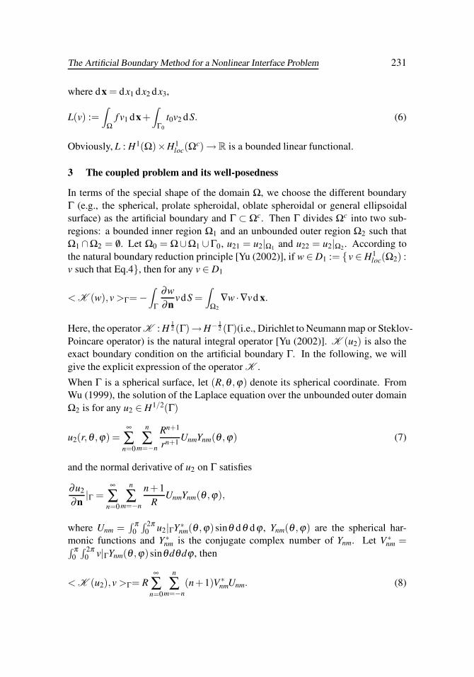
When Γ is a spherical surface, let (R,θ ,ϕ) denote its spherical coordinate. FromWu (1999), the solution of the Laplace equation over the unbounded outer domainΩ2 is for any u2 ∈ H1/2(Γ)
u2(r,θ ,ϕ) =∞
∑n=0
n
∑m=−n
Rn+1
rn+1 UnmYnm(θ ,ϕ) (7)
and the normal derivative of u2 on Γ satisfies
∂u2
∂n|Γ =
∞
∑n=0
n
∑m=−n
n+1R
UnmYnm(θ ,ϕ),
where Unm =∫ π
0
∫ 2π0 u2|ΓY∗
nm(θ ,ϕ) sinθ dθ dϕ , Ynm(θ ,ϕ) are the spherical har-monic functions and Y∗
nm is the conjugate complex number of Ynm. Let V ∗nm =∫ π
0
∫ 2π0 v|ΓYnm(θ ,ϕ) sinθdθdϕ , then
< K (u2),v >Γ= R∞
∑n=0
n
∑m=−n
(n+1)V ∗nmUnm. (8)
232 Copyright © 2008 Tech Science Press CMES, vol.35, no.3, pp.227-252, 2008
When Γ is a spheroidal surface{(x1,x2,x3) : (x21 +x2
2)/a2+x23/b2 = 1}(If a > b, Γ is
oblate; If a < b, Γ is prolate.) and (μ1,θ ,ϕ) denotes its oblate or prolate spheroidalcoordinate, let
Tnm(μ) =
⎧⎪⎪⎨⎪⎪⎩−dQm
n (coshμ)/dμQm
n (coshμ)sinhμ , for Γ is prolate spheroidal surface
−dT mn (sinhμ)/d μT m
n (sinhμ)coshμ , for Γ is oblate spheroidal surface
where Qmn (x) denote the associated Legendre functions of the second kind and
T mn (x) = iexp(
iπn2
)Qmn (ix), i2 = −1.
From Huang (2007), for the prolate spheroidal surface, the solution of the Laplaceequation over the unbounded outer domain Ω2 is
u(μ ,θ ,ϕ) =∞
∑n=0
n
∑m=−n
Qmn (coshμ)
Qmn (coshμ1)
UnmYnm (9)
and the normal derivative of u2 on Γ satisfies
∂u2
∂n|Γ =
−∞
∑n=0
n
∑m=−n
Tnm(μ1)UnmYnm
f0
√cosh2 μ1 −cos2 θ
and for the oblate spheroidal surface, the solution of the Laplace equation over theunbounded outer domain Ω2 is
u(μ ,θ ,ϕ) =∞
∑n=0
n
∑m=−n
T mn (sinhμ)
T mn (sinhμ1)
UnmYnm (10)
and the normal derivative of u2 on Γ satisfies
∂u2
∂n|Γ =
−∞
∑n=0
n
∑m=−n
Tnm(μ1)UnmYnm
f0
√cosh2 μ1 − sin2 θ
.
Thus, we obtain
< K (u2),v >Γ= f0
∞
∑n=0
n
∑m=−n
Tnm(μ1)V ∗nmUnm, (11)
The Artificial Boundary Method for a Nonlinear Interface Problem 233
where f0 =√|a2−b2|, Ynm, Unm and V ∗
nm are the same as the above definition forthe spherical surface.
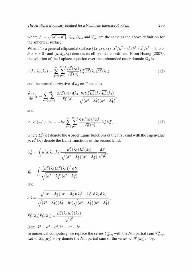
When Γ is a general ellipsoidal surface {(x1,x2,x3) : x21/a2+x2
2/b2+x23/c2 = 1, a >
b > c > 0} and (a,λ2,λ3) denotes its ellipsoidal coordinate. From Huang (2007),the solution of the Laplace equation over the unbounded outer domain Ω2 is
u(λ1,λ2,λ3) =∞
∑n=0
2n+1
∑p=1
F pn (λ1)
F pn (a)
U pn E p
n (λ2)E pn (λ3) (12)
and the normal derivative of u2 on Γ satisfies
∂u2
∂n|Γ =
∞
∑n=0
2n+1
∑p=1
dF pn (a)/dλ1
F pn (a)
bcU pn E p
n (λ2)E pn (λ3)√
(a2−λ 22 )(a2−λ 2
3 ),
and
< K (u2),v >Γ= −bc∞
∑n=0
2n+1
∑p=1
dF pn (a)/dλ1
F pn (a)
U pn V p
n , (13)
where E pn (λ ) denote the n order Lamé functions of the first kind with the eigenvalue
p, F pn (λ ) denote the Lamé functions of the second kind,
U pn =
∫Γ
u(a,λ2,λ3)E p
n (λ2)E pn (λ3)√
(a2−λ 22 )(a2−λ 2
3 )
dS√γ p
n
,
γ pn =
∫Γ
(E p
n (λ2)E pn (λ3)
)2dS√
(a2 −λ 22 )(a2−λ 2
3 )
and
dS =
√(a2 −λ 2
2 )(a2−λ 23 )(λ 2
2 −λ 23 )dλ2 dλ3√
(k2−λ 22 )(λ 2
2 −h2)√
(k2 −λ 23 )(h2−λ 2
3 ),
E pn (λ2)E p
n (λ3) =E p
n (λ2)E pn (λ3)√
γ pn
.
Here, k2 = a2 −c2,h2 = a2 −b2.
In numerical computing, we replace the series ∑∞n=0 with the Nth partial sum ∑N
n=0.Let < KN(u2),v >Γ denote the Nth partial sum of the series < K (u2),v >Γ.
234 Copyright © 2008 Tech Science Press CMES, vol.35, no.3, pp.227-252, 2008
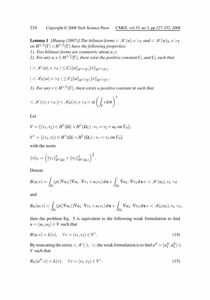
Lemma 1 [Huang (2007)] The bilinear forms < K (u),v >Γ and < K (u)N,v >Γon H1/2(Γ)×H1/2(Γ) have the following properties:1). Two bilinear forms are symmetric about u,v.2). For any u,v ∈ H1/2(Γ), there exist the positive constant C1 and C2 such that
| < K (u),v >Γ | ≤C1‖u‖H1/2(Γ)‖v‖H1/2(Γ),
| < KN(u),v >Γ | ≤C2‖u‖H1/2(Γ)‖v‖H1/2(Γ).
3). For any v ∈ H1/2(Γ), there exists a positive constant α such that
< K (v),v >Γ≥< KN(v),v >Γ> α(∫
Γvdσ
)2
.
Let
V = {(v1,v2) ∈ H1(Ω)×H1(Ω1) : v1 = v2 +u0 on Γ0},
V ∗ = {(v1,v2) ∈ H1(Ω)×H1(Ω1) : v1 = v2 on Γ0}with the norm
‖v‖V =(‖v1‖2
H1(Ω) +‖v2‖2H1(Ω1)
) 12.
Denote
B(u;v) =∫
Ω(p(|∇u1|)∇u1 ·∇v1 +u1v1)dx+
∫Ω1
∇u2 ·∇v2 dx+ < K (u2),v2 >Γ
and
BN(u;v) =∫
Ω(p(|∇u1|)∇u1 ·∇v1 +u1v1)dx+
∫Ω1
∇u2 ·∇v2 dx+ < KN(u2),v2 >Γ,
then the problem Eq. 5 is equivalent to the following weak formulation to findu = (u1,u2) ∈V such that
B(u;v) = L(v), ∀v = (v1,v2) ∈V ∗. (14)
By truncating the series < K (·), ·>, the weak formulation is to find uN = (uN1 ,uN
2 )∈V such that
BN(uN ;v) = L(v), ∀v = (v1,v2) ∈ V ∗. (15)
The Artificial Boundary Method for a Nonlinear Interface Problem 235
In order to obtain the existence and uniqueness of solution of the original interfaceproblem, we must give the Euler equations of the problem Eq. 14 and Eq. 15.Define Φ : V → R by
Φ(u) :=∫
Ω(g(|∇u1|)+
12|u1|2)dx+
12
∫Ω1
|∇u2|2 dx+12
< K (u2),u2 >Γ −L(u),
where
g : [0,∞) → [0,∞), t −→ g(t) =∫ t
0sp(s)ds.
Clearly, 12 p0t2 ≤ g(t)≤ 1
2 p1t2. Thus, for any u ∈ H1(Ω),
G(u) :=∫
Ωg(|∇u|)dx
is bounded. Let
ΦN(u) = G(u1)+∫
Ω
12|u1|2 dx+
12
∫Ω1
|∇u2|2 dx+12
< KN(u2),u2 >Γ −L(u),
then the coupled minimization problem is to find u = (u1,u2) ∈V such that
Φ(u) = infv∈V
Φ(v). (16)
The approximate minimization problem is to find uN = (uN1 ,uN
2 ) ∈ V such that
ΦN(uN) = infv∈V
ΦN(v). (17)
In the following, we refer to Carstensen and Gwinner (1997) and discuss the well-posedness of the problem Eq. 16 and Eq. 17.
Lemma 2 For any u ∈ V and v ∈ V ∗, the following conclusions hold.1). The Gateaux derivative of Φ is
DΦ(u;v) = B(u;v)−L(v). (18)
2). DΦ is strongly monotone and Lipschitz-continuous for the bounded argumentswith respect to the norm ‖ · ‖V [see Ciarlet (1978)].
Proof. For any u ∈V and v ∈V ∗, p(t) ∈ C1({0}∪R+) implies
limt→0
Φ(u+ tv)−Φ(u)t
=∫
Ωp(|∇u1|)∇u1 ·∇v1 dx+
∫Ω
u1v1 dx+∫
Ω1
∇u2 ·∇v2 dx
+ < K (u2),v >Γ −L(v).
236 Copyright © 2008 Tech Science Press CMES, vol.35, no.3, pp.227-252, 2008
Since∣∣∣∣∫
Ωp(|∇u|)∇u ·∇vdx
∣∣∣∣≤ p1
∫Ω|∇u||∇v|dx ≤ p1‖∇u‖L2(Ω)‖v‖H1(Ω),
for a fixed u, DΦ(u;v)−L(v) is a bounded linear functional on V ∗. This solves 1).Similarly, we can obtain
D2Φ(u;v;w) =∫
Ω
((∇v1)TE(∇u1)∇w1 +w1v1
)dx
+∫
Ω1
∇w2 ·∇v2 dx+ < K (w2),v2 >Γ
with the 3×3-unit matrix I3×3 and
E(t) := p(t)I3×3 + t p′(t)(sign t) · (sign t)T ∈ R3×3,
where t ∈ R3; t := |t|, signt is the unit vector with respect to the direction t. Three
eigenvalues of the matrix E(t) are t p′(t)+ p(t) and p(t) (double). Since t p′(t)+p(t) > α > 0 and p(t) > p0 > 0, E(t) is symmetric positive definite. Then D2Φ(u;v;w)with respect to w is still a bounded linear functional on V ∗. For all u,w ∈ V , thereis t1 ∈ (0,1) such that
DΦ(u;u−w)−DΦ(w;u−w) = D2Φ(w+ t1(u−w);u−w;u−w).
Thus, Friedrichs inequality and the properties of the matrix E(t) satisfy
DΦ(u;u−w)−DΦ(w;u−w) ≥C1‖u1−w1‖2H1(Ω)
+|u2 −w2|2H1(Ω1) +C2
(∫Γ(u2 −w2)dσ
)2
≥C(‖u1 −w1‖2
H1(Ω) +‖u2 −w2‖2H1(Ω1)
)
and for any bounded ball B(0;M) = {w ∈V : ‖w‖V ≤ M}, we have
DΦ(u;u−w)−DΦ(w;u−w) ≤C(‖u1−w1‖2
H1(Ω) +‖u2 −w2‖2H1(Ω1)
).
Theorem 1 The functional Φ has a unique minimizer on V and the minimizer isjust the unique solution of the weak formulation Eq. 14. The functional ΦN has aunique minimizer on V and the minimizer is just the unique solution of the weakformulation Eq. 15.
The Artificial Boundary Method for a Nonlinear Interface Problem 237
Proof. Given u0 ∈ H1/2(Γ0), there exists u1 ∈ H1(Ω) with u1|Γ0 = u0. Takingu2 = 0 in H1(Ω1), we obtain u = (u1,u2) ∈ V and Φ(u) < ∞, that is to say V �= /0and if Φ has a minimizer on V , then the minimizer must be finite. Obviously,V is also closed and convex. In the following, we prove that Φ is weakly lowersemicontinuous in V . For all u ∈ V , if the sequence {un}∞
1 weakly converge to u ,then the monotonicity of DΦ and the Taylor formula of Φ imply that there exists at ∈ (0,1), such that
Φ(un)−Φ(u) = DΦ(u+ t(un−u);un −u) ≥ DΦ(u;un−u).
Since DΦ(u;w) with respect to w is a linear bounded functional on V ∗, we haveDΦ(u;un−u) → 0 and then Φ is weakly lower semicontinuous in V . On the otherhand, for any v = (v1,v2)∈V , Frierichs inequality and the properties of p(t) satisfy
Φ(v)≥ C1‖v1‖2H1(Ω) +C2‖v2‖2
H1(Ω1) −‖ f‖L2(Ω)‖v1‖L2(Ω)−‖t0‖H−1/2(Γ0)‖v2‖H1/2(Γ0).
Thus,
lim‖v‖V →∞
v∈V
Φ(v) = +∞.
i.e., for given w ∈V , there exists a positive constant M such that
‖v‖V > M ⇒ Φ(v) ≥ Φ(w), ∀v ∈V.
According to the concerned conclusions [Ciarlet (1978)], Φ has at most one min-imizer on V . Let u = (u1,u2) ∈ V is the minimizer of Φ on V , for any ±v ∈ V ∗,lemma 2 implies that
0 ≤ limt→0+
Φ(u± tv)−Φ(u)t
= ±(B(u;v)−L(v)).
Thus, u = (u1,u2) must be the solution of the weak formulation Eq. 14. Conversely,if u = (u1,u2) is the solution of the weak formulation Eq. 14, then for all w ∈ V ,Gateaux differential of Φ and the strong monotonicity of DΦ(w;v) with respect tow imply that there exists t ∈ (0,1) such that
Φ(w)−Φ(u) = DΦ(u+ t(w−u);w−u) ≥ DΦ(u;w−u) = 0.
Hence, u is the minimizer of Φ on V . Finally, we prove the uniqueness. Supposethat u,w are both the solution of the weak formulation Eq. 14, then we have
B(u;u−w)−B(w;u−w) = 0.
238 Copyright © 2008 Tech Science Press CMES, vol.35, no.3, pp.227-252, 2008
u = w follows from the strong monotonicity of DΦ. This proves that the functionalΦ has a unique minimizer on V and the minimizer is just the unique solution ofthe variational problem Eq. 14. Similarly, we obtain that the functional ΦN has aunique minimizer on V and the minimizer is just the unique solution of the varia-tional problem Eq. 15.
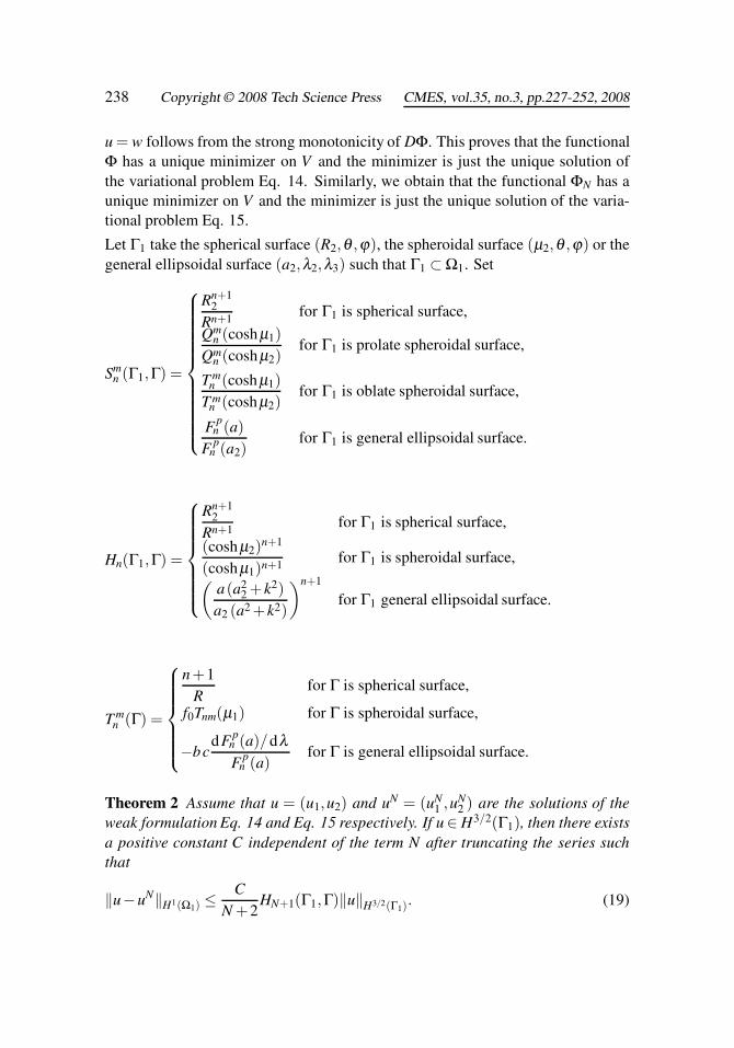
Let Γ1 take the spherical surface (R2,θ ,ϕ), the spheroidal surface (μ2,θ ,ϕ) or thegeneral ellipsoidal surface (a2,λ2,λ3) such that Γ1 ⊂ Ω1. Set
Smn (Γ1,Γ) =
⎧⎪⎪⎪⎪⎪⎪⎪⎪⎪⎪⎪⎨⎪⎪⎪⎪⎪⎪⎪⎪⎪⎪⎪⎩
Rn+12
Rn+1 for Γ1 is spherical surface,
Qmn (coshμ1)
Qmn (coshμ2)
for Γ1 is prolate spheroidal surface,
T mn (coshμ1)
T mn (coshμ2)
for Γ1 is oblate spheroidal surface,
F pn (a)
F pn (a2)
for Γ1 is general ellipsoidal surface.
Hn(Γ1,Γ) =
⎧⎪⎪⎪⎪⎪⎪⎨⎪⎪⎪⎪⎪⎪⎩
Rn+12
Rn+1 for Γ1 is spherical surface,
(coshμ2)n+1
(coshμ1)n+1 for Γ1 is spheroidal surface,(a(a2
2 +k2)a2 (a2 +k2)
)n+1
for Γ1 general ellipsoidal surface.
T mn (Γ) =
⎧⎪⎪⎪⎪⎪⎨⎪⎪⎪⎪⎪⎩
n+1R
for Γ is spherical surface,
f0Tnm(μ1) for Γ is spheroidal surface,
−bcdF p
n (a)/dλF p
n (a)for Γ is general ellipsoidal surface.
Theorem 2 Assume that u = (u1,u2) and uN = (uN1 ,uN
2 ) are the solutions of theweak formulation Eq. 14 and Eq. 15 respectively. If u∈ H3/2(Γ1), then there existsa positive constant C independent of the term N after truncating the series suchthat
‖u−uN‖H1(Ω1) ≤C
N +2HN+1(Γ1,Γ)‖u‖H3/2(Γ1). (19)
The Artificial Boundary Method for a Nonlinear Interface Problem 239
Proof. Because u = (u1,u2) and uN = (uN1 ,uN
2 ) are the solutions of Eq. 14 and Eq.15 respectively, for any v ∈ V ∗, we have
B(u;v)−BN(uN;v) = 0.
From lemma 2 and lemma 1, there exists a positive constant C1 independent of Nsuch that
C1‖u−uN‖2V ≤ BN(u;u−uN)−BN(uN ;u−uN)
= BN(u;u−uN)−B(u;u−uN)= < KN(u)−K (u),u−uN >Γ .
Let Fnm, Unm and Pnm are the generalized Fourier coefficient of (u−uN)|Γ, u|Γ andu|Γ1, respectively, then we have
< KN(u),u−uN >Γ − < K (u),u−uN >Γ
≤∞
∑n=N+1
n
∑m=−n
T mn (Γ)|Unm||Fnm|
≤C‖u−uN‖H1/2(Γ)
(∞
∑n=N+1
n
∑m=−n
(n+1)|Unm|2) 1
2
The formula Eq. 7, Eq. 9, Eq. 10,
Unm = Smn (Γ1,Γ)Pnm.
Therefore,
‖u−uN‖V ≤ C
(∞
∑n=N+1
n
∑m=−n
(n+1)|Unm|2) 1
2
≤ C
(∞
∑n=N+1
n
∑m=−n
(n+1)3
(N +2)2 (Smn Γ1,Γ)2|Pnm|2
) 12
≤ CN +2
HN+1(Γ1,Γ)‖u‖H3/2(Γ1).
Here, C is independent of N.
4 Discrete problem and error estimate
To describe a discrete formulation of Eq. 16 and Eq. 17, we divide Ω and Ω1
into quasi-uniform regular tetrahedral meshes with mesh size h, such that the nodes
240 Copyright © 2008 Tech Science Press CMES, vol.35, no.3, pp.227-252, 2008
on Γ0 are matching (i.e., coincident) and these tetrahedrons nearby Γ are curved.The conforming linear finite element spaces associated with Ω and Ω1 are denotedby Vh(Ω) and Vh(Ω1) respectively. Usually, the curved tetrahedrons are approxi-mated by the straight edge tetrahedrons which have the same nodes as the curvedtetrahedrons. This approximate only generates small error. Letting Nh denotethe set of nodes in the domain Ω∪Ω1 ∪∂Ω∪∂Ω1, we let Uh = {vh = (vh
1,vh2) ∈
Vh(Ω)×Vh(Ω1) : ∀b ∈ Nh ∩Γ0,vh1(b) = vh
2(b) + u0(b)}, U∗h = {vh = (vh
1,vh2) ∈
Vh(Ω)×Vh(Ω1) : ∀b ∈ Nh ∩Γ0,vh1(b) = vh
2(b)}. Then, we have U∗h ⊂V ∗.
The discrete formulation of the problem Eq. 14 is to find uh = (uh1,uh
2) ∈ Uh suchthat
B(uh;vh) = L(vh), ∀vh ∈ U∗h . (20)
The discrete formulation of the problem Eq. 15 is to find uNh = (uNh1 ,uNh
2 ) ∈ Uh
such that
BN(uNh;vh) = L(vh), ∀vh ∈U∗h . (21)
Theorem 3 The discrete problem Eq. 20 and Eq. 21 both exist a unique solution.
The proof is similar with the proof of theorem 1.
Suppose that the interpolation operator Πh : H2(Ω∪Ω1∪Γ0) →Uh such that inter-polation error
|v−Πhv|H1(Ω) ≤ Ch|v|H2(Ω), ∀v ∈ H2(Ω)
and
|v−Πhv|H1(Ω1) ≤Ch|v|H2(Ω1), ∀v ∈ H2(Ω1).
Theorem 4 Assume that u and uNh are the solution of the problem Eq. 14 and Eq.21 respectively, and u ∈ H2(Ω)×H2(Ω1) and u|Γ1 ∈ H3/2(Γ1), then there exists apositive constant C independent of the mesh size h and the term N after truncatingthe series such that
‖u−uNh‖V ≤C(
h‖u‖H2(Ω)×H2(Ω1) +(
1N +2
HN+1(Γ1,Γ)‖u‖H3/2(Γ1)
).
Proof. Let uN = (uN1 ,uN
2 ) is the solution of the problem Eq. 15. Owing to U∗h ∈V ∗,
we have
BN(uN ;vh)−BN(uNh;vh) = 0, ∀vh ∈U∗h .
The Artificial Boundary Method for a Nonlinear Interface Problem 241
For any wh ∈Uh, wh −uNh ∈U∗h . The strong monotonicity and Lipschitz continuity
about the bounded variable of DΦ satisfy
C1‖uN −uNh‖2V ≤ BN(uN −uNh;uN −uNh)
= BN(uN −uNh;uN −wh)≤ C2‖uN −uNh‖V‖uN −wh‖V
Namely,
‖uN −uNh‖V ≤C infwh∈Uh
‖uN −wh‖V .
Thus, theorem 2 implies that
‖u−uNh‖V ≤ ‖u−uN‖V +‖uN −uNh‖V
≤ ‖u−uN‖V +C‖uN −Πhu‖V
≤ (1+C)‖u−uN‖V +C‖u−Πhu‖V
≤ C
(h‖u‖H2(Ω)×H2(Ω1) +
1N +2
HN+1(Γ1,Γ)‖u‖H3/2(Γ1)
).
Remark. The above error estimate indicates that Nopt = ln(h)/ ln(coshμ2/cosh μ1)−2 may be chosen as the optimal truncation term with respect to the norm in H1,when the mesh size is fixed.
5 Numerical examples
In numerical computation, we first do harmonic extension of u0 to Ω1. Let vh0 ∈
Vh(Ω1) be the weak solution of the following problem⎧⎨⎩
Δvh0 = 0, in Ω1,
vh0 = u0, on Γ0,
vh0 = 0, on Γ.
Set
L(vh) = L(vh)+∫
Ω1
∇vh2 ·∇vh
0 dx.
Clearly, L(vh) is still the bounded linear functional on U∗h . Thus, solve numerically
the following problem: find wNh = (uNh1 ,wNh
2 ) ∈U∗ such that
BN(wNh;vh) = L(vh), ∀vh ∈ U∗. (22)
242 Copyright © 2008 Tech Science Press CMES, vol.35, no.3, pp.227-252, 2008
If wNh = (uNh1 ,wNh
2 ) is the unique solution of the problem Eq. 22, then uNh =(uNh
1 ,wNh2 −vh
0) must be the unique solution of the problem Eq. 21. Conversely, theconclusion is also hold.
To solve the nonlinear problem Eq. 22, we apply Newton iteration. Let e1(h,N) =‖uNh −u‖H1(Ωs), e0(h,N) = ‖uNh −u‖L2(Ωs), e∞(h,N) = ‖uNh −u‖L∞(Ωs). Here, ifs = 0, the domain Ωs denotes Ω; if s = 1, the domain Ωs denotes Ω1. iters, nodesand tetra denote the times of Newton iteration, the total number of the nodes in Ωs
and the total number of the tetrahedrons elements, respectively. Error in Fig. 8and Fig. 14 denotes the norm of uNh−u50h in three spaces as the mesh size is fixedwhile Error in Fig. 19 denotes the norm of uNh − u20h in three spaces. In otherfigures, Error denotes the norm of u−uNh. According to the special shape of theinner domain Ω, we apply the different artificial boundary, e.g., a spherical, prolatespheroidal, oblate spheroidal and general ellipsoidal surface.
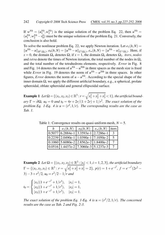
Example 1 Let Ω = {(x1,x2,x3)∈R3 : r =
√x2
1 +x22 +x2
3 < 1}, the artificial bound-
ary Γ = ∂Ω, u0 = 0 and t0 = 4r + 2r/(1+ 2r)+ 1/r2. The exact solution of theproblem Eq. 1-Eq. 4 is u = (r2,1/r). The corresponding results are the case asTab. 1.
Table 1: Convergence results on quasi-uniform mesh, N = 5.
h e1(h,N) e0(h,N) e∞(h,N) iters0.5077 6.2884e-1 3.3593e-1 2.7286e-1 30.2239 2.0490e-1 1.0390e-1 7.1050e-2 50.1060 5.6080e-2 2.8562e-2 1.8400e-2 70.0516 1.4437e-2 7.3060e-3 5.1237e-3 7
Example 2 Let Ω = {(x1,x2,x3) ∈ R3 : |xi|< 1, i = 1,2,3}, the artificial boundary
Γ = {(x1,x2,x3) ∈ R3 : r =
√x2
1 +x22 +x2
3 = 2}, p(t) = 1 + e−t2, f = e−r2
(2r2 −3)−3+ r2/2, u0 = r2/2−1/r and
t0 =
⎧⎪⎨⎪⎩
|x1|(1+e−r2+1/r3), |x1| = 1,
|x2|(1+e−r2+1/r3), |x2| = 1,
|x3|(1+e−r2+1/r3), |x3| = 1.
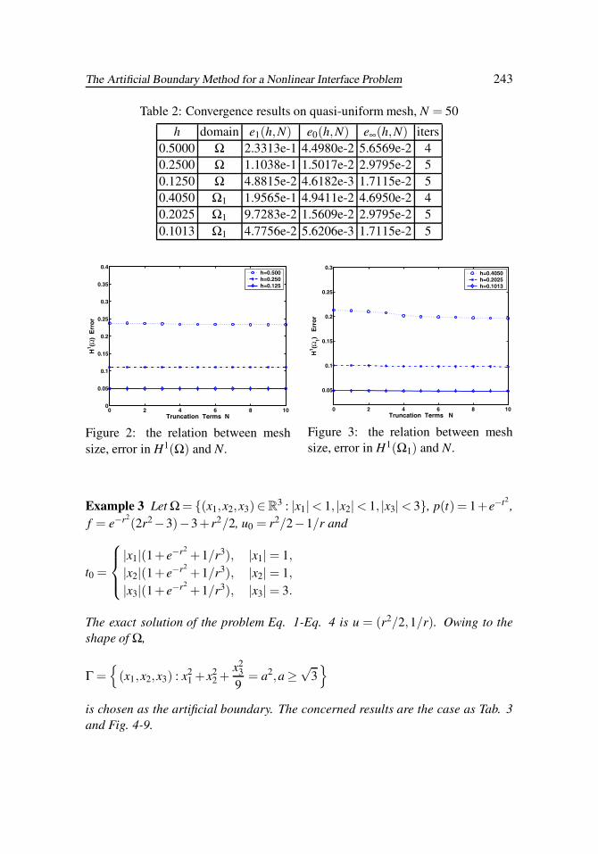
The exact solution of the problem Eq. 1-Eq. 4 is u = (r2/2,1/r). The concernedresults are the case as Tab. 2 and Fig. 2-3.
The Artificial Boundary Method for a Nonlinear Interface Problem 243
Table 2: Convergence results on quasi-uniform mesh, N = 50
h domain e1(h,N) e0(h,N) e∞(h,N) iters0.5000 Ω 2.3313e-1 4.4980e-2 5.6569e-2 40.2500 Ω 1.1038e-1 1.5017e-2 2.9795e-2 50.1250 Ω 4.8815e-2 4.6182e-3 1.7115e-2 50.4050 Ω1 1.9565e-1 4.9411e-2 4.6950e-2 40.2025 Ω1 9.7283e-2 1.5609e-2 2.9795e-2 50.1013 Ω1 4.7756e-2 5.6206e-3 1.7115e-2 5
0 2 4 6 8 100
0.05
0.1
0.15
0.2
0.25
0.3
0.35
0.4
Truncation Terms N
H1 (Ω
) E
rro
r
h=0.500h=0.250h=0.125
Figure 2: the relation between meshsize, error in H1(Ω) and N.
0 2 4 6 8 10
0.05
0.1
0.15
0.2
0.25
0.3
Truncation Terms N
H1 (Ω
1) E
rro
r
h=0.4050h=0.2025h=0.1013
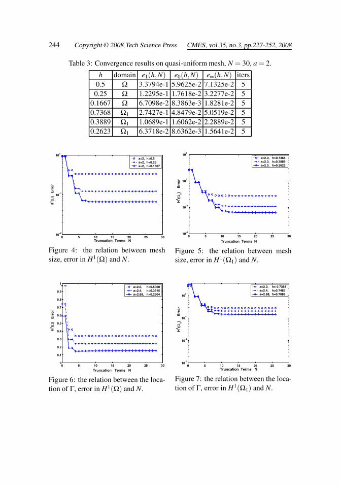
Figure 3: the relation between meshsize, error in H1(Ω1) and N.
Example 3 Let Ω = {(x1,x2,x3)∈R3 : |x1|< 1, |x2|< 1, |x3|< 3}, p(t) = 1+e−t2
,f = e−r2
(2r2−3)−3+ r2/2, u0 = r2/2−1/r and
t0 =
⎧⎪⎨⎪⎩
|x1|(1+e−r2+1/r3), |x1| = 1,
|x2|(1+e−r2+1/r3), |x2| = 1,
|x3|(1+e−r2+1/r3), |x3| = 3.
The exact solution of the problem Eq. 1-Eq. 4 is u = (r2/2,1/r). Owing to theshape of Ω,
Γ ={
(x1,x2,x3) : x21 +x2
2 +x2
3
9= a2,a ≥
√3}
is chosen as the artificial boundary. The concerned results are the case as Tab. 3and Fig. 4-9.
244 Copyright © 2008 Tech Science Press CMES, vol.35, no.3, pp.227-252, 2008
Table 3: Convergence results on quasi-uniform mesh, N = 30, a = 2.
h domain e1(h,N) e0(h,N) e∞(h,N) iters0.5 Ω 3.3794e-1 5.9625e-2 7.1325e-2 50.25 Ω 1.2295e-1 1.7618e-2 3.2277e-2 5
0.1667 Ω 6.7098e-2 8.3863e-3 1.8281e-2 50.7368 Ω1 2.7427e-1 4.8479e-2 5.0519e-2 50.3889 Ω1 1.0689e-1 1.6062e-2 2.2889e-2 50.2623 Ω1 6.3718e-2 8.6362e-3 1.5641e-2 5
0 5 10 15 20 25 3010
−2
10−1
100
Truncation Terms N
H1 (Ω
) E
rro
r
a=2, h=0.5a=2, h=0.25a=2, h=0.1667
Figure 4: the relation between meshsize, error in H1(Ω) and N.
0 5 10 15 20 25 3010
−2
10−1
100
101
Truncation Terms N
H1 (Ω
1)
Err
or
a=2.0, h=0.7368 a=2.0, h=0.3889a=2.0, h=0.2622
Figure 5: the relation between meshsize, error in H1(Ω1) and N.
0 5 10 15 20 25 300
0.1
0.2
0.3
0.4
0.5
0.6
0.7
0.8
0.9
1
Truncation Terms N
H1 (Ω
) E
rro
r
a=2.0, h=0.5000a=2.4, h=0.3915a=2.88, h=0.2904
Figure 6: the relation between the loca-tion of Γ, error in H1(Ω) and N.
0 5 10 15 20 25 3010
−3
10−2
10−1
100
Truncation Terms N
H1 (Ω
1)
Err
or
a=2.0, h= 0.7368a=2.4, h=0.7483a=2.88, h=0.7086
Figure 7: the relation between the loca-tion of Γ, error in H1(Ω1) and N.
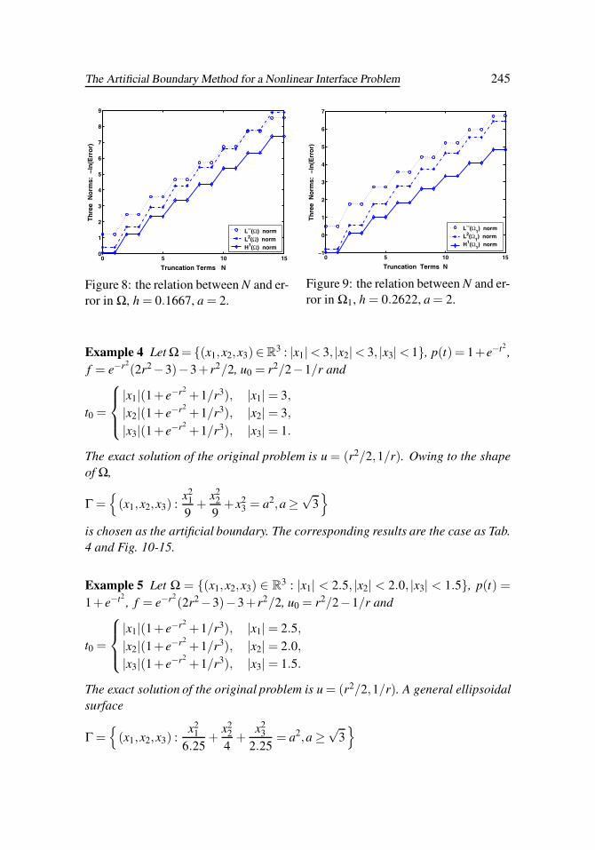
The Artificial Boundary Method for a Nonlinear Interface Problem 245
0 5 10 150
1
2
3
4
5
6
7
8
9
Truncation Terms N
Th
ree
No
rms:
−ln
(Err
or)
L∞(Ω) normL2(Ω) norm H1(Ω) norm
Figure 8: the relation between N and er-ror in Ω, h = 0.1667, a = 2.
0 5 10 15−1
0
1
2
3
4
5
6
7
Truncation Terms N
Th
ree
No
rms:
−ln
(Err
or)
L∞(Ω1) norm
L2(Ω1) norm
H1(Ω1) norm
Figure 9: the relation between N and er-ror in Ω1, h = 0.2622, a = 2.
Example 4 Let Ω = {(x1,x2,x3)∈R3 : |x1|< 3, |x2|< 3, |x3|< 1}, p(t) = 1+e−t2
,f = e−r2
(2r2−3)−3+ r2/2, u0 = r2/2−1/r and
t0 =
⎧⎪⎨⎪⎩
|x1|(1+e−r2+1/r3), |x1| = 3,
|x2|(1+e−r2+1/r3), |x2| = 3,
|x3|(1+e−r2+1/r3), |x3| = 1.
The exact solution of the original problem is u = (r2/2,1/r). Owing to the shapeof Ω,
Γ ={
(x1,x2,x3) :x2
1
9+
x22
9+x2
3 = a2,a ≥√
3}
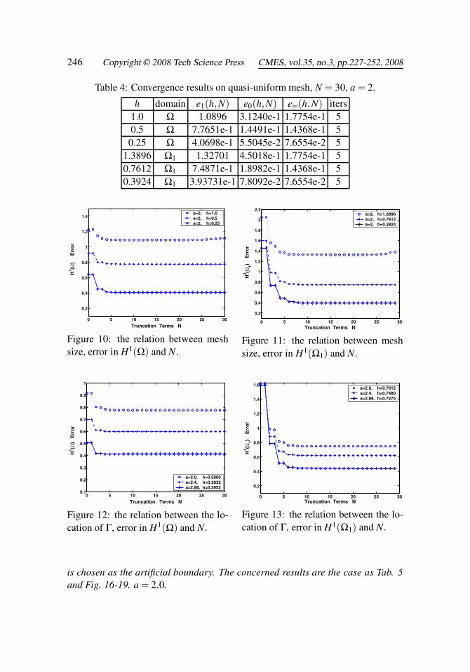
is chosen as the artificial boundary. The corresponding results are the case as Tab.4 and Fig. 10-15.
Example 5 Let Ω = {(x1,x2,x3) ∈ R3 : |x1| < 2.5, |x2| < 2.0, |x3| < 1.5}, p(t) =
1+e−t2, f = e−r2
(2r2−3)−3+ r2/2, u0 = r2/2−1/r and
t0 =
⎧⎪⎨⎪⎩
|x1|(1+e−r2+1/r3), |x1| = 2.5,
|x2|(1+e−r2+1/r3), |x2| = 2.0,
|x3|(1+e−r2+1/r3), |x3| = 1.5.
The exact solution of the original problem is u = (r2/2,1/r). A general ellipsoidalsurface
Γ ={
(x1,x2,x3) :x2
1
6.25+
x22
4+
x23
2.25= a2,a ≥
√3}
246 Copyright © 2008 Tech Science Press CMES, vol.35, no.3, pp.227-252, 2008
Table 4: Convergence results on quasi-uniform mesh, N = 30, a = 2.
h domain e1(h,N) e0(h,N) e∞(h,N) iters1.0 Ω 1.0896 3.1240e-1 1.7754e-1 50.5 Ω 7.7651e-1 1.4491e-1 1.4368e-1 50.25 Ω 4.0698e-1 5.5045e-2 7.6554e-2 5
1.3896 Ω1 1.32701 4.5018e-1 1.7754e-1 50.7612 Ω1 7.4871e-1 1.8982e-1 1.4368e-1 50.3924 Ω1 3.93731e-1 7.8092e-2 7.6554e-2 5
0 5 10 15 20 25 30
0.2
0.4
0.6
0.8
1
1.2
1.4
Truncation Terms N
H1 (Ω
)
Err
or
a=2, h=1.0a=2, h=0.5a=2, h=0.25
Figure 10: the relation between meshsize, error in H1(Ω) and N.
0 5 10 15 20 25 30
0.2
0.4
0.6
0.8
1
1.2
1.4
1.6
1.8
2
2.2
Truncation Terms N
H2 (Ω
1)
Err
or
a=2, h=1.3896a=2, h=0.7612a=2, h=0.3924
Figure 11: the relation between meshsize, error in H1(Ω1) and N.
0 5 10 15 20 25 300.1
0.2
0.3
0.4
0.5
0.6
0.7
0.8
0.9
1
Truncation Terms N
H1 (Ω
) E
rro
r
a=2.0, h=0.5000a=2.4, h=0.3832a=2.88, h=0.2952
Figure 12: the relation between the lo-cation of Γ, error in H1(Ω) and N.
0 5 10 15 20 25 30
0.2
0.4
0.6
0.8
1
1.2
1.4
1.6
Truncation Terms N
H1 (Ω
1)
Err
or
a=2.0, h=0.7612a=2.4, h=0.7480a=2.88, h=0.7275
Figure 13: the relation between the lo-cation of Γ, error in H1(Ω1) and N.
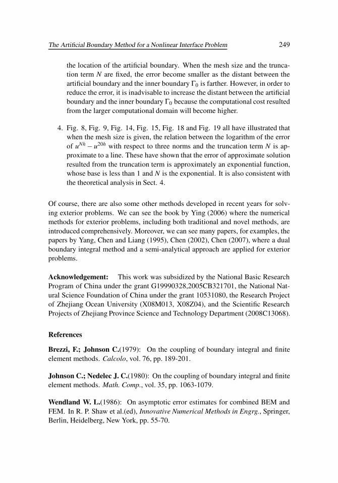
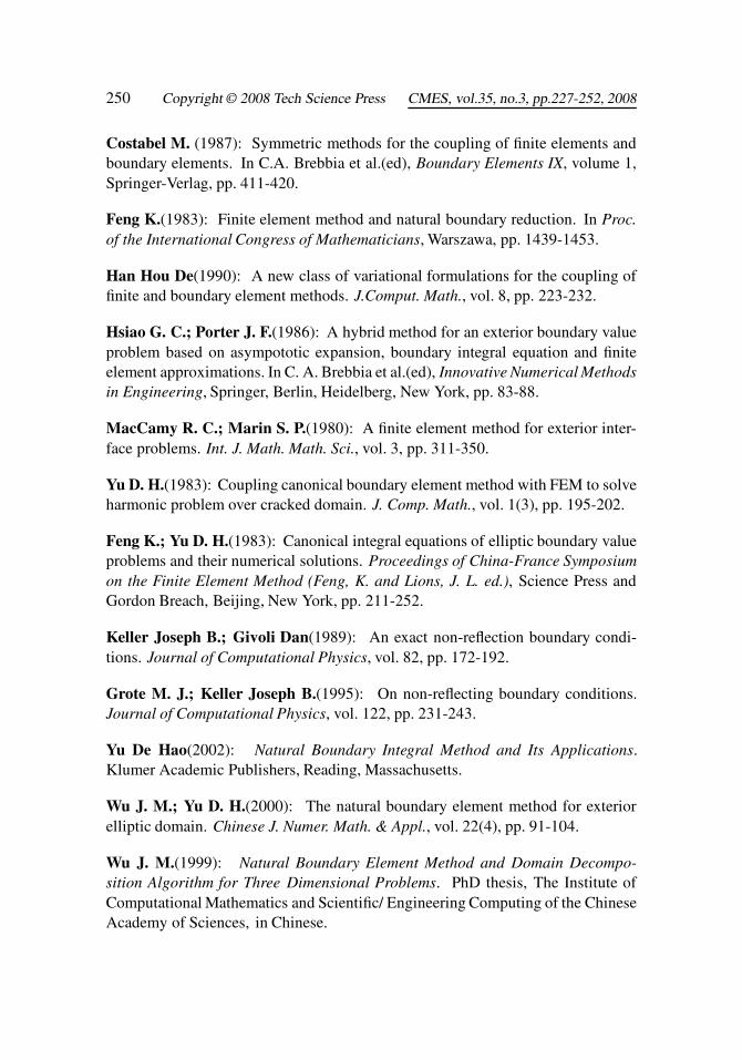
is chosen as the artificial boundary. The concerned results are the case as Tab. 5and Fig. 16-19. a = 2.0.
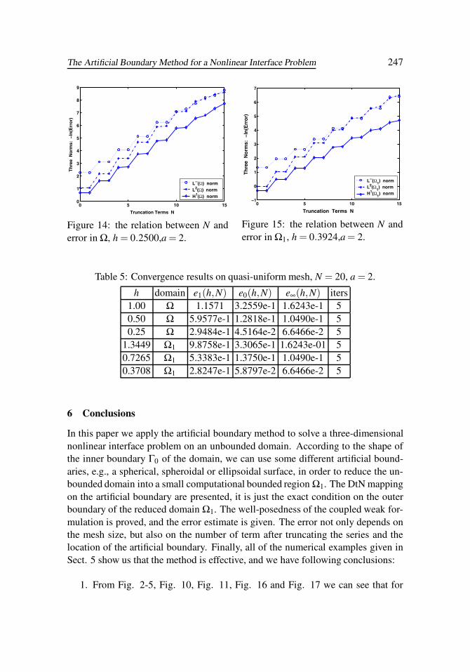
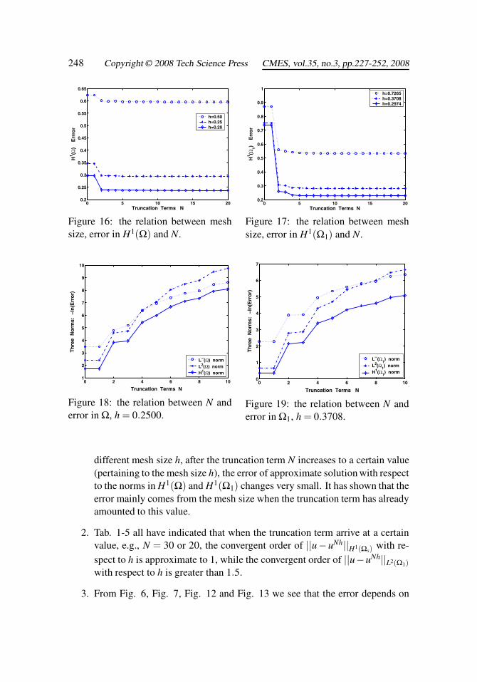
The Artificial Boundary Method for a Nonlinear Interface Problem 247
0 5 10 150
1
2
3
4
5
6
7
8
9
Truncation Terms N
Th
ree
No
rms:
−ln
(Err
or)
L∞(Ω) normL2(Ω) norm H1(Ω) norm
Figure 14: the relation between N anderror in Ω, h = 0.2500,a = 2.
0 5 10 15−1
0
1
2
3
4
5
6
7
Truncation Terms N
Th
ree
No
rms:
−ln
(Err
or)
L∞(Ω1) norm
L2(Ω1) norm
H1(Ω1) norm
Figure 15: the relation between N anderror in Ω1, h = 0.3924,a = 2.
Table 5: Convergence results on quasi-uniform mesh, N = 20, a = 2.
h domain e1(h,N) e0(h,N) e∞(h,N) iters1.00 Ω 1.1571 3.2559e-1 1.6243e-1 50.50 Ω 5.9577e-1 1.2818e-1 1.0490e-1 50.25 Ω 2.9484e-1 4.5164e-2 6.6466e-2 5
1.3449 Ω1 9.8758e-1 3.3065e-1 1.6243e-01 50.7265 Ω1 5.3383e-1 1.3750e-1 1.0490e-1 50.3708 Ω1 2.8247e-1 5.8797e-2 6.6466e-2 5
6 Conclusions
In this paper we apply the artificial boundary method to solve a three-dimensionalnonlinear interface problem on an unbounded domain. According to the shape ofthe inner boundary Γ0 of the domain, we can use some different artificial bound-aries, e.g., a spherical, spheroidal or ellipsoidal surface, in order to reduce the un-bounded domain into a small computational bounded region Ω1. The DtN mappingon the artificial boundary are presented, it is just the exact condition on the outerboundary of the reduced domain Ω1. The well-posedness of the coupled weak for-mulation is proved, and the error estimate is given. The error not only depends onthe mesh size, but also on the number of term after truncating the series and thelocation of the artificial boundary. Finally, all of the numerical examples given inSect. 5 show us that the method is effective, and we have following conclusions:
1. From Fig. 2-5, Fig. 10, Fig. 11, Fig. 16 and Fig. 17 we can see that for
248 Copyright © 2008 Tech Science Press CMES, vol.35, no.3, pp.227-252, 2008
0 5 10 15 200.2
0.25
0.3
0.35
0.4
0.45
0.5
0.55
0.6
0.65
Truncation Terms N
H1 (Ω
)
Err
ror
h=0.50h=0.25h=0.20
Figure 16: the relation between meshsize, error in H1(Ω) and N.
0 5 10 15 200.2
0.3
0.4
0.5
0.6
0.7
0.8
0.9
1
Truncation Terms N
H1 (Ω
1)
Err
or
h=0.7265h=0.3708h=0.2974
Figure 17: the relation between meshsize, error in H1(Ω1) and N.
0 2 4 6 8 101
2
3
4
5
6
7
8
9
10
Truncation Terms N
Th
ree
No
rms:
−ln
(Err
or)
L∞(Ω) normL2(Ω) normH1(Ω) norm
Figure 18: the relation between N anderror in Ω, h = 0.2500.
0 2 4 6 8 100
1
2
3
4
5
6
7
Truncation Terms N
Th
ree
No
rms:
−ln
(Err
or)
L∞(Ω1) norm
L2(Ω1) norm
H1(Ω1) norm
Figure 19: the relation between N anderror in Ω1, h = 0.3708.
different mesh size h, after the truncation term N increases to a certain value(pertaining to the mesh size h), the error of approximate solution with respectto the norms in H1(Ω) and H1(Ω1) changes very small. It has shown that theerror mainly comes from the mesh size when the truncation term has alreadyamounted to this value.
2. Tab. 1-5 all have indicated that when the truncation term arrive at a certainvalue, e.g., N = 30 or 20, the convergent order of ||u−uNh||H1(Ωs) with re-spect to h is approximate to 1, while the convergent order of ||u−uNh||L2(Ω1)with respect to h is greater than 1.5.
3. From Fig. 6, Fig. 7, Fig. 12 and Fig. 13 we see that the error depends on
The Artificial Boundary Method for a Nonlinear Interface Problem 249
the location of the artificial boundary. When the mesh size and the trunca-tion term N are fixed, the error become smaller as the distant between theartificial boundary and the inner boundary Γ0 is farther. However, in order toreduce the error, it is inadvisable to increase the distant between the artificialboundary and the inner boundary Γ0 because the computational cost resultedfrom the larger computational domain will become higher.
4. Fig. 8, Fig. 9, Fig. 14, Fig. 15, Fig. 18 and Fig. 19 all have illustrated thatwhen the mesh size is given, the relation between the logarithm of the errorof uNh − u20h with respect to three norms and the truncation term N is ap-proximate to a line. These have shown that the error of approximate solutionresulted from the truncation term is approximately an exponential function,whose base is less than 1 and N is the exponential. It is also consistent withthe theoretical analysis in Sect. 4.
Of course, there are also some other methods developed in recent years for solv-ing exterior problems. We can see the book by Ying (2006) where the numericalmethods for exterior problems, including both traditional and novel methods, areintroduced comprehensively. Moreover, we can see many papers, for examples, thepapers by Yang, Chen and Liang (1995), Chen (2002), Chen (2007), where a dualboundary integral method and a semi-analytical approach are applied for exteriorproblems.
Acknowledgement: This work was subsidized by the National Basic ResearchProgram of China under the grant G19990328,2005CB321701, the National Nat-ural Science Foundation of China under the grant 10531080, the Research Projectof Zhejiang Ocean University (X08M013, X08Z04), and the Scientific ResearchProjects of Zhejiang Province Science and Technology Department (2008C13068).
References
Brezzi, F.; Johnson C.(1979): On the coupling of boundary integral and finiteelement methods. Calcolo, vol. 76, pp. 189-201.
Johnson C.; Nedelec J. C.(1980): On the coupling of boundary integral and finiteelement methods. Math. Comp., vol. 35, pp. 1063-1079.
Wendland W. L.(1986): On asymptotic error estimates for combined BEM andFEM. In R. P. Shaw et al.(ed), Innovative Numerical Methods in Engrg., Springer,Berlin, Heidelberg, New York, pp. 55-70.
250 Copyright © 2008 Tech Science Press CMES, vol.35, no.3, pp.227-252, 2008
Costabel M. (1987): Symmetric methods for the coupling of finite elements andboundary elements. In C.A. Brebbia et al.(ed), Boundary Elements IX, volume 1,Springer-Verlag, pp. 411-420.
Feng K.(1983): Finite element method and natural boundary reduction. In Proc.of the International Congress of Mathematicians, Warszawa, pp. 1439-1453.
Han Hou De(1990): A new class of variational formulations for the coupling offinite and boundary element methods. J.Comput. Math., vol. 8, pp. 223-232.
Hsiao G. C.; Porter J. F.(1986): A hybrid method for an exterior boundary valueproblem based on asympototic expansion, boundary integral equation and finiteelement approximations. In C. A. Brebbia et al.(ed), Innovative Numerical Methodsin Engineering, Springer, Berlin, Heidelberg, New York, pp. 83-88.
MacCamy R. C.; Marin S. P.(1980): A finite element method for exterior inter-face problems. Int. J. Math. Math. Sci., vol. 3, pp. 311-350.
Yu D. H.(1983): Coupling canonical boundary element method with FEM to solveharmonic problem over cracked domain. J. Comp. Math., vol. 1(3), pp. 195-202.
Feng K.; Yu D. H.(1983): Canonical integral equations of elliptic boundary valueproblems and their numerical solutions. Proceedings of China-France Symposiumon the Finite Element Method (Feng, K. and Lions, J. L. ed.), Science Press andGordon Breach, Beijing, New York, pp. 211-252.
Keller Joseph B.; Givoli Dan(1989): An exact non-reflection boundary condi-tions. Journal of Computational Physics, vol. 82, pp. 172-192.
Grote M. J.; Keller Joseph B.(1995): On non-reflecting boundary conditions.Journal of Computational Physics, vol. 122, pp. 231-243.
Yu De Hao(2002): Natural Boundary Integral Method and Its Applications.Klumer Academic Publishers, Reading, Massachusetts.
Wu J. M.; Yu D. H.(2000): The natural boundary element method for exteriorelliptic domain. Chinese J. Numer. Math. & Appl., vol. 22(4), pp. 91-104.
Wu J. M.(1999): Natural Boundary Element Method and Domain Decompo-sition Algorithm for Three Dimensional Problems. PhD thesis, The Institute ofComputational Mathematics and Scientific/ Engineering Computing of the ChineseAcademy of Sciences, in Chinese.
The Artificial Boundary Method for a Nonlinear Interface Problem 251
Huang H. Y.(2007): An artificial boundary method for three-dimensional prob-lems over unbounded domain with an ellipsoidal artificial boundary. PhD thesis,Academy of Mathematics and System Sciences of the Chinese Academy of Sci-ences, in Chinese.
Yu D. H.(1985): Approximation of boundary conditions at infinity for a harmonicequation. J. Comp. Math., vol. 3(3), pp. 219-227.
Du Q. K.; Yu D. H.(2000): The coupled method based on natural boundary re-duction for parabolic equation. Computational Physics, vol. 17(6), pp. 593-601, inChinese.
Du Q. K.; Yu D. H.(2001): On the natural integral equation for initial bound-ary value problems of two dimensional hyperbolic equation. Acta MathematicaeApplicatae Sinica, vol. 24(1), pp. 17-26.
Liu Y.(2007): Solution of Some Electromagnetic Problems Based on NaturalBoundary Elements and Domain Decomposition Method. PhD thesis, Academyof Mathematics and System Sciences of the Chinese Academy of Sciences, inChinese.
Hu Q. Y.; Yu D. H.(2001): A solution method for a certain nonlinear interfaceproblem in unbounded domains. Computing, vol. 67, pp. 119-140.
Huang H. Y.; Yu D. H.(2006): Natural boundary element method for three di-mensional exterior harmonic problem with an inner prolate spheriod boundary. J.Comput. Math., vol. 24(2), pp. 193-208.
Feistauer M.(1985): Mathematical and numerical study of nonlinear problems influid mechanics. In M. Zlámal J. Vosmanshy(ed), Proc. Conf. Equadiff 6, Springer,pp. 3-16.
Feistauer M.(1987): On the finite element approximation of a cascade flow prob-lem. Numer. Math., vol. 50, pp. 655-684.
Carstensen Carsten; Gwinner Joachim(1997): FEM and BEM coupling for anonlinear transmission problem with Signorini contact. SIAM J.Numer.Anal., vol.34, pp. 1845-1864.
Costabel M. M.; Stephan E. P.(1990): Coupling of finite and boundary elementmethods for an elastoplastic interface problem. SIAM J. Numer. Anal., vol. 27(5),pp. 1212-1226.
252 Copyright © 2008 Tech Science Press CMES, vol.35, no.3, pp.227-252, 2008
Stephan E. P.(1992): Coupling of finite elements and boundary elements for somenonlinear interface problems. Comput. Methods Appl. Mech. Engrg., vol. 101, pp.61-72.
Lions J. L.; Magenes E.(1972): Non-Homogeneous Boundary Value Problemsand Applications, volume I. Springer-Verlag, New York.
Ciarlet P. G.(1978): The Finite Element Method for Elliptic Problems. North-Holland Publishing Company, New York.
Ying L. A.(2006): Numerical Methods for Exterior Problems. World Scientific,New Jersey.
Yang S. S.; Chen J. T.; Liang M. T.(1995): Dual boundary integral equations forexterior problems. Engrg. Anal. with Boundary Elements, vol. 16, pp. 333-340.
Chen C. T.; Chen J. T.; Chen K. H.(2002): Adaptive boundary element method oftime-harmonic exterior acoustics in two dimensions. Computer Methods in AppliedMechanics and Engineering, vol. 191, pp. 3331-3345.
Chen P. Y.; Chen I. L.; Chen J. T.; Chen C. T.(2007): A semi-analytical approachfor radiation and scattering problems with circular boundaries. Computer Methodsin Applied Mechanics and Engineering, vol. 196, pp. 2751-2764.
Liu Chein-Shan(2007): A meshless regularized integral equation method forlaplace equation in arbitrary interior or exterior plane domains. CMES: ComputerModeling in Engineering & Sceinces, vol. 19(1), pp. 99-109.
Jr. Soares Delfim(2008): A time-domain fem-bem iterative coupling algorithm tonumerically model the propagation of electromagnetic waves. CMES: ComputerModeling in Engineering & Sceinces, vol. 32(2), pp. 57-68.
Novati G.; Springhetti R.; Margonari M.(2006): Weak coupling of the symmet-ric galerkin bem with fem for potential and elastostatic problems. CMES: ComputerModeling in Engineering & Sceinces, vol. 13(1), pp. 67-80.