The arrangement field of the space-time points

Diego Marin∗, Fabrizio Coppola, Marcello Colozzo

Pangea Association†and Istituto Scientia‡

November 6, 2018

Abstract

In this paper we introduce the concept of “non-ordered space-time”.

We formulate the quantum field theory over such a non-ordered generalized

space. The imposition of an order over an non-ordered space automatically

generates gravity, which appears as a fictitious force. We then uncover an

unexpected, close relationship between gravity and quantum entanglement.

Keywords: Quantum gravity, Non-locality, Entanglement, EPR paradox, Quan-

tum measurement, Theory of everything.

∗dmarin.math@gmail.com†www.gruppopangea.com, Via A. Manzoni 18, 36065, Mussolente (VI), Italy‡www.istitutoscientia.it, Via Ortola 65, 54100, Massa (MS), Italy

1

arX

iv:1

201.

3765

v5 [

phys

ics.

gen-

ph]

4 A

pr 2

012

1 Introduction

In section 2 we start with a historical overview of the concepts of space and time,

exposing the philosophical idea of non-ordered space-time.

In section 3 we begin to develop the mathematics that implements this idea.

In section 4.3 we extend the concept of derivative on a non-ordered space (we

use “space” in its larger meaning of space-time). We derive the scalar field action

for such a space. In this process, the original derivative operator (∂ or ∇) is

replaced by a field M , which we call “Arrangement Field”.

In section 4.3.1 we show that the scalar field action for a non-ordered space is

equal to the standard scalar field action for an ordered space with metric h.

h is uniquely determined by M . In a non-ordered space we can quantize the

field M with no problems. Quantizing M automatically quantizes h.

We see that a non-ordered space naturally provides gauge invariance for U(∞)

transformations. Consequently, in an ordered space, the M field collapses into the

covariant derivative ∇ = ∂ + A, with U(∞) gauge fields.

In section 4.3.2 we add to the action other two U(∞)-invariant terms, which

lead back to the Hilbert-Einstein and Gauss-Bonnet terms in ordered space. These

two terms give a potential for M , whose minimum corresponds to a precise ar-

rangement of the space-time points. We see how this minimum breaks the U(∞)

symmetry, generating masses for the gauge fields, according to a mechanism that

is different from the Higgs one. We conjecture that the residual symmetry of the

minimum corresponds to the standard model symmetry.

In section 5.1 we show how the existence of M separates the other fields into two

categories, bosons and fermions, reproducing the usual rules of (anti)commutation,

without introducing exotic concepts as Grassmann variables. Furthermore, M

creates connections between pairs (or groups) of particles, generating the usual

phenomenon of quantum entanglement.

In section 5.2 we see that a natural extension of the Hilbert-Einstein term in a

2

non-ordered space gives the standard action for fermion fields.

Finally, in section 8, we see that the M field, in some cases, simulates a mea-

surement operation, acting on the others fields (or on itself) as a projector.

3

Contents

1 Introduction 2

2 Historical and philosophical excursus 6

2.1 Classical Physics . . . . . . . . . . . . . . . . . . . . . . . . . . . . 6

2.2 Space and Time according to Kant and other philosophers . . . . . 7

2.3 Relativistic physics . . . . . . . . . . . . . . . . . . . . . . . . . . . 9

2.4 Quantum limitation of objectivity . . . . . . . . . . . . . . . . . . 12

2.5 Uncertainty, observables, entanglement, non-locality . . . . . . . . 14

2.6 Explaining both entanglement and gravity . . . . . . . . . . . . . . 19

3 A non-ordered universe 21

3.1 Reciprocal relationship between space-time points . . . . . . . . . . 21

3.2 The Matrix relating couples of points . . . . . . . . . . . . . . . . 23

3.3 The origin of the space-time metric . . . . . . . . . . . . . . . . . . 26

3.4 The origin of entanglement and particle mass . . . . . . . . . . . . 28

3.5 Measurement, Spin, Bosons, Fermions, Strings . . . . . . . . . . . . 30

4 The arrangement of the space-time points 33

4.1 1-dimensional model . . . . . . . . . . . . . . . . . . . . . . . . . . 34

4.2 Extending the model to many dimensions . . . . . . . . . . . . . . . 41

4.2.1 The Arrangement Matrix . . . . . . . . . . . . . . . . . . . . 41

4.3 Physical interpretation . . . . . . . . . . . . . . . . . . . . . . . . . 46

4.3.1 The scalar field action in a non-ordered space-time . . . . . 46

4.3.2 Quantization of the field M . . . . . . . . . . . . . . . . . . 54

4.3.3 A final hypothesis: quantization of field M substitutes grav-

ity quantization . . . . . . . . . . . . . . . . . . . . . . . . 57

4.3.4 Superimposition . . . . . . . . . . . . . . . . . . . . . . . . . 62

5 Antisymmetric, symmetric and trace components 66

4

5.1 Commutation relations. Bosonic and fermionic fields . . . . . . . . 76

5.2 Fermionic action . . . . . . . . . . . . . . . . . . . . . . . . . . . . 78

6 Quantum Entanglement 81

6.1 Bohm interpretation . . . . . . . . . . . . . . . . . . . . . . . . . . 81

6.2 Quantum Entanglement in the M field framework . . . . . . . . . 85

7 The trace term and the mass of the fields 87

8 Measurement of a quantum observable 88

9 Physical consequences 94

9.1 Non-commutative geometry . . . . . . . . . . . . . . . . . . . . . . 94

9.2 Entropy . . . . . . . . . . . . . . . . . . . . . . . . . . . . . . . . . 95

9.3 Inflation . . . . . . . . . . . . . . . . . . . . . . . . . . . . . . . . . 95

A Partition of R1 96

B The (+1) (−1) form 99

B.1 Passage to the continuous . . . . . . . . . . . . . . . . . . . . . . . 101

C Topological Spaces 103

D Measurement of a quantum observable: degenerate eigenvalues 108

D.1 Reduction of the state vector . . . . . . . . . . . . . . . . . . . . . 109

E Measurement of a quantum observable (example) 110

5

2 Historical and philosophical excursus

2.1 Classical Physics

According to classical physics, space and time are absolute and fundamental enti-

ties. In analyzing the events taking place in the universe, it is assumed that the

extension of space and the flowing of time form a preordained structure, within

which the interactions between physical objects can occur. Moreover, the physical

properties of a body or system are supposed to be objective and independent of a

possible observation made by a scientist or any conscious being. In this paradigm,

reality exists independently of classical measurements and is not significantly in-

fluenced by them: it is supposed that an observation of a system does not alter

its physical characteristics, unless it is particularly “invasive”or implies remark-

able operational influences. Even in highly “invasive”cases, however, it is natural

to assume that the observed object had its own pre-existing characteristics, not

determined by the process of observation.

In this view it is obvious that space and time are “absolute”and the observation

of a physical system does not significantly alter its properties: these are implicit

tenets of classical physics, which are usually extended to whole science, in its

continuous development towards universality and pure objectivity. Such a purpose

appeared to have got solid foundations in the structure of space-time, considered

as an unchangeable, perfect, huge four-dimensional lattice that fills the universe

and represents the theater where all the events occur, compared to which, the

figure of the observer and the act of measurement are practically irrelevant.

Since we live in the objective universe, we can act on nearby objects and

possibly modify them, but we can not operate directly on space or time: at most

we are allowed to “occupy”some parts of space during certain periods of time,

but, apart from that, space and time appear as “unavoidably”imposed over us,

regardless of our will. These considerations are accepted by the majority of human

beings and appear natural, obvious or even trivial.

6

2.2 Space and Time according to Kant and other philoso-

phers

Despite the rapid and successful development of classical physics and science in

general, firmly based on the (supposedly) stable nature of space and time, a num-

ber of respectable philosophers, starting from the end of the seventeenth century

(when modern science had already taken the first steps) until the beginning of

the nineteenth century (when science was definitely established), including Locke,

Hume, Leibniz, Kant and Schopenhauer, conceptualized and described space and

time not as objective, universal entities, independent from the conscious human be-

ings, but as concepts defined by our own intellect and intuition, aimed to perceive

and interpret the external reality. This point of view was significantly different

from the conception of classical physics, based on objectivity, and appeared quite

extravagant to many scientists of that time. Nevertheless, Kant, whose knowledge

in astronomy, mathematics, anatomy and other sciences was not negligible, was

able to expose his conception in a profound, logical, rational way.

Kant distinguishes two main activities of conscious mind: “analytic proposi-

tions”and “synthetic propositions”. In an oversimplified interpretation, analytic

propositions are the elements of rational, logical reasoning, in which thoughts

proceed by deduction, starting from known facts and finding consequences that,

anyway, were implicit in the premises and only had to made explicit by reason-

ing. Synthetic propositions, instead, are new, non-deductible informations, coming

from perceptions and sensations. We can not deduce (for instance) if an apple is

sweet, or a radiator is hot: we must check it through our senses.

Kant also proposed another distinction, between: “a priori”propositions, that

means “in advance”, ie “before ”an experience in the external world is performed;

and “a posteriori”propositions, that means “after”an experience. According to

Kant, all analytic propositions must be ”a priori”. A trivial example is the follow-

ing addition: 5 + 7 = 12. This analytic proposition is true “a priori”: the result

7

was already 12 even before we did the calculation. Therefore, Kant affirms that

no analytic proposition can be “a posteriori”. Synthetic propositions, on the other

side, are generally “a posteriori”, since perceptions come from experience.

Now, an interesting question arises: may “a priori”synthetic propositions ex-

ist? The unexpected answer by Kant is: yes, they may and do exist. For ex-

ample, certain “categories”that human mind applies to objects or events are “a

priori”synthetic propositions. The principle of cause-effect, according to Kant, is

an “a priori”synthetic form, because we perceive certain events from the external

world and then we relate them to each other, according to a category (causality)

that already exists (“a priori”) in our intellect, independently from the experience.

According to Kant, the most important “a priori”synthetic forms are space and

time. There is no doubt that they are related to experience. Nevertheless Kant

states that they are not inherent to the objective phenomena, but are subjective

tools that our intellect uses to order the experiences. The “a priori”forms of space

and time fulfill such purpose so efficiently that we attribute them to the external

word itself, rather than to our own intuition.

Despite Kant’s brilliant descriptions, the extraordinary results obtained by

classical, mechanistic physics between 1600 and 1900 appeared to be in an ir-

reconcilable conflict with such a philosophy, and seemed to confirm the “solid

materiality”and “objective persistence”of the ”objective” world. Space and time

really appeared as absolute structures on which “objective”reality was actually

based, whereas the considerations by Kant and the other mentioned philosophers

appeared as charming, but unrealistic, unfounded and misleading lucubrations.

In the early twentieth century, however, physics started to face unexpected

problems and contradictions, so that the physicists were forced to postulate and

accept new principles and radical changes.

8

2.3 Relativistic physics

In 1632 Galileo intuited and enunciated the “principle of relativity”, stating that

the laws of physics are the same in all possible inertial reference systems [1]. Later

developments of physics, including several discoveries in optics and electromag-

netism, suggested instead that a privileged, fundamental reference system should

exist, even though this was in contradiction with Galileo’s principle. This prob-

lem especially affected electrodynamics, that was an excellent theory under many

aspects, but also included unsolved inconsistencies.

In 1905 Einstein was able to solve the whole problem by restarting from the

Galileo’s principle of relativity and applying it to the new knowledge of electromag-

netism and optics, thus developing an original, consistent theory, called “special

relativity”[2].

No one better than him could explain the problem, just before solving it: “It

is known that Maxwell’s electrodynamics [...] when applied to moving bodies, leads

to asymmetries which do not appear to be inherent in the phenomena. Take, for

example, the reciprocal electrodynamic action of a magnet and a conductor. The

observable phenomenon here depends only on the relative motion of the conductor

and the magnet, whereas the customary view draws a sharp distinction between the

two cases in which either the one or the other of these bodies is in motion. For if

the magnet is in motion and the conductor at rest, there arises in the neighbourhood

of the magnet an electric field with a certain definite energy, producing a current at

the places where parts of the conductor are situated. But if the magnet is stationary

and the conductor in motion, no electric field arises in the neighbourhood of the

magnet. In the conductor, however, we find an electromotive force, to which in

itself there is no corresponding energy, but which gives rise [...] to electric currents

of the same path and intensity as those produced by the electric forces in the former

case ”.

More formally, Maxwell’s equations include the current density J , which is not

invariant in different inertial reference systems. Einstein also reports the historical

9

experiment made by Michelson and Morley [3] in 1887, which showed that the

speed of light did not follow the classical laws of velocity addition [4], also due to

Galileo (1638), like common objects do. Specifically, Michelson and Morley proved

that the speed of light is not affected by the different Earth’s vector velocity at

different times during its annual orbit:

“Examples of this sort, together with the unsuccessful attempts to discover any

motion of the Earth relatively to the ’light medium’, suggest that the phenomena

of electrodynamics as well as of mechanics possess no properties corresponding to

the idea of absolute rest. They suggest rather that [...] the same laws of electrody-

namics and optics will be valid for all frames of reference for which the equations

of mechanics hold good. We will raise this conjecture (the purport of which will

hereafter be called the ’Principle of Relativity’) to the status of a postulate, and

also introduce another postulate [...] that light is always propagated in empty space

with a definite velocity c which is independent of the state of motion of the emitting

body. These two postulates suffice for the attainment of a simple and consistent

theory of the electrodynamics of moving bodies.”

Accepting these postulates, no privileged frame of reference could exist, and

all inertial systems were equivalent, as was already realized by Galileo in 1632.

However, Einstein’s theory also implied a new, unusual and counterintuitive idea:

that time flows differently in different inertial reference systems, and the perception

of space is also different depending on the reference system where the observer

stands. In light of such unexpected advances, we can say that Kant’s ideas were

not so extravagant, after all. Furthermore, Einstein postulated that the speed of

light, symbolized by c, is invariant in every inertial reference system, since it is not

subjected to composition with other velocities.

Thus time and space lose their absolute characteristics if considered indepen-

dently from each other, but, adequately considered as components (coordinates)

of four-dimensional points, remain “absolute”as a single entity defined as space-

time. This generalized geometrical entity includes time as a fourth coordinate (in

10

addition to the three spatial ones), thus forming the four-dimensional geometrical

structure also called chronotope.

The four-dimensional space-time points were called “events”, following the orig-

inal paper by Einstein [2]. In 1908 this four-dimensional structure was perfected

and defined as Minkowski space [5], and the “Lorentz transformations”corrected

the old “Galilean transformations”used since 1638 for velocity addition (and still

today for non-relativistic applications).

As we know, the speed of light is very high, so that in a given reference system,

in order to accelerate a material object to speeds comparable to c, a huge amount of

energy is required, which becomes higher as the speed increases, until the purpose

proves to be impractical: the required energy becomes, to the limit, infinite. The

constant c in physics thus became an insurmountable speed limit and was assumed

to be an universal physical constant.

In 1916 Einstein expanded the principle of relativity to non-inertial systems,

therefore defining his new theory of “general relativity”, which led to a description

of the universe in terms of a four-dimensional geometry, curved by the presence

of the masses [6], so that even the (linear) Minkowski space had to be considered

as an approximation, valid only in small regions of the curved universe. In this

new perspective, the so-called “gravitational forces”find their natural explanation

in purely geometrical terms, based on a complex concept of metric. This further-

more affects the structure of space and time, making more difficult to follow the

development of the physical chains of cause-effect, to the point that Einstein, in

section a2, wrote (1916): “The law of causality has not the significance of a state-

ment as to the world of experience, except when observable facts ultimately appear

as causes and effects” [6]. Kant had exposed this apparent “extravagance”about

causality a long time before.

11

2.4 Quantum limitation of objectivity

Starting from 1905, the year in which Einstein proposed the theory of special

relativity, a rapid succession of discoveries occurred, specifically during the next

three decades, when the concept of “objectivity”of physical events was somehow

weakened by the development of quantum mechanics (QM). Quantum theory was

born in 1900 with the hypothesis proposed by Planck [7] to solve an important

problem in thermodynamics of radiation, specifically about the electromagnetic

emission of the black body. Planck postulated that the activity of matter at very

small scales, ie at molecular and atomic levels, occurred through “leaps”of energy,

so that the radiation was emitted not uniformly but by discrete amounts, called

“quanta”of light, or “photons”. Einstein, in 1905 (the same year he formulated

the theory of special relativity) utilized the concept of Planck in order to explain

the so-called photoelectric effect [8] in which light was also absorbed by quanta

(besides being emitted by quanta as in the Planck’s case of the black body).

During the following years, important details over the internal structure of

atoms started to emerge: in 1911 Rutherford showed that most of the mass of the

atom resides in the small nucleus, around which the electrons (much lighter than

the nucleus) somehow “orbit”[9]. Rutherford’s experiment represented a major

step for the development of atomic physics, the gradual process to understand

the atoms, their structure and behavior, much of which consists of activity and

interaction with light and other electromagnetic radiations. Each chemical element

can emit and absorb light (or electromagnetic radiation) at specific frequencies

(corresponding to specific wavelengths) that are characteristics of the chemical

under consideration and distinct from the other ones. Physicists could measure

those wavelengths with remarkable precision, but did not understand the laws

that determined them. Nevertheless,they were aware that such phenomena were

produced at the atomic level.

Summarizing, the atomic phenomena involved different disciplines such as op-

tics, electromagnetism, thermodynamics, general physics and chemistry, but none

12

of these sciences could provide a proper explanation of the observed results.

In 1913 Bohr proposed a model of the atom [10] that eventually was able to

explain a large amount of the experimental data, almost all the data collected in

spectroscopy during the previous decades, especially regarding hydrogen and other

light gases: in such cases the accuracy of the theory was excellent, matching the

experimental data with an extraordinary precision (although in the case of heavier

atoms the situation was not as good, so that certain corrections were necessary).

Bohr had been inspired by the Rutherford’s discovery occurred two years earlier

and by the concept of “quantum”that both Planck in 1900 and Einstein in 1905 had

already successfully applied to atomic phenomena involving light. Bohr, however,

did not impose quantization on energy directly (either of emitted or absorbed

photons) like in the two previous cases, but proposed to quantize the angular

momentum of the electrons in their (alleged) orbits around the nucleus. Making

calculations, consequently energy also resulted distributed in discrete, quantized

levels.

By applying this principle to the simplest atom in nature, hydrogen, whose

nucleus is a single (positively electrically charged) proton, around which a (neg-

atively charged) electron somehow “moves”(in a different way than it would do

according to classical physics), Bohr calculated the quantized series of levels for

the possible values of energy of the electron. The respective differences between

the different levels accurately matched and explained the spectra shown by light

in spectroscopy. However, in the case of more complex and heavier gases, the

mathematical frame became more difficult, the results were less precise, and the

agreement between theory and experimental data was approximative. Neverthe-

less, it was clear that the theoretical development of this new theory was going in

the right direction.

The “Bohr model”had shown that quantization was not exclusively related to

energy, but could be applied to the angular momentum of electrons in atoms,

demonstrating it was more important and general than Planck and Einstein them-

13

selves had realized. The Bohr model was a turning point for the development

of quantum mechanics (QM), which gradually was able to describe virtually all

the phenomena of microscopic systems, such as molecules, atoms and subatomic

particles, making QM the foundation of atomic and nuclear physics.

The results provided by the Bohr model were not yet complete: in the case

of heavier atoms many details could not be explained. The laborious subsequent

researches (mainly conducted by the Copenhagen School directed by Bohr himself

during the 1920’s) made the theory mathematically more precise, but intuitively

abstruse and incomprehensible. There was no clear view of the motion of the

electrons around the atomic nucleus.

2.5 Uncertainty, observables, entanglement, non-locality

While developing the quantum theory, it began to emerge that the experiments

inevitably influenced the observed systems. At one point, Bohr, Heisenberg and

other physicists of the so-called “Copenhagen school”(from the city of Bohr) be-

gan to suspect that the physical properties of particles and quantum systems could

no longer be assumed to be completely predefined and ontologically independent

from the observation. In the first version of the so-called “Copenhagen interpreta-

tion”they assumed that the will of the conscious observer (the scientist performing

the experiment) played a decisive role in the collapse of a quantum state into a

single eigenstate [11].

This appeared as an unacceptable extravagance to many physicists, including

Einstein, since the supposed objectivity of the universe happened to face unex-

pected restrictions. During the classical age many physicists were astronomers

also, including Galileo and Newton, so that their natural attitude while observ-

ing distant stars implicitly included the conviction that there was no possibility

whatsoever for the observer to influence the observed body. Such a conviction of

a purely objective universe continued to dominate scientists’ attitude and their

vision of reality, also when ordinary objects of daily life were examined, and even

14

when physics began to deal with microscopic objects such as molecules and atoms.

However, quantum systems are actually described by states that do not neces-

sarily contain all the information that is usually attributed to classical, macroscopic

systems. A quantum state is generally defined by a mathematical superimposi-

tion of eigenstates, that evolves deterministically, but remains devoided of certain

characteristics, which can only be revealed (objectivated) when the quantum state

collapses (in probabilistic terms rather than deterministically, as pointed out by

Born [12] in 1926), into an “eigenstate”of the measured physical quantity. This

is the reason why the physical quantities in QM are called “observables”: they

generally remain in a virtual, abstract state, even if they evolve following an exact

and deterministic law discovered in 1926, the Schrodinger equation [13], but retain

several of their physical properties unrevealed, until they are objectively observed.

The unusual fact is that the theory works fine only if such hidden properties are

not objectively defined before the measurement, and are partly created by the act

of observations itself, when the state collapses (or is reduced) to an eigenstate. At

that point, the observable actually reveals a definite value, in excellent agreement

with one of the possible outcomes (eigenvalues) according to calculations based

on QM theory, which can not provide an exact prediction, though. Despite the

quantized eigenvalues can be calculated with extraordinary precision, QM can not

predict which one among the possible eigenstates will come out, but only provides

the probability for the outcome of each eigenstate.

So, the quantum realm seems to exist mostly in undefined, non-completely

objective states, since the number of eigenstates is much lower than the number

of generic states. Moreover, eigenstates are usually different depending on which

physical quantity (“observable”) is measured.

A fairly accurate measurement of the position of a particle (usually denoted by q)

implies an inaccurate measurement of its velocity v, since the small uncertainty

∆q about the position must have a relationship with the uncertainty ∆p over the

momentum, according to the Heisenberg uncertainty principle (1927), ∆p∆q ≥ ~2.

15

The uncertainty principle [14] puts an end to the absolute determinism that

seemed implicit in classical physics. The rigid cause-effect chains now admit a

margin of “uncertainty”, in which Nature seems to reserve a small room for Her

non-predictable “caprice”or (according to Jordan, Pauli, Wigner, Eddington and

other scientists) “willingness”[15].

Another important consequence is created by the act of measurement. The

subsequent course of the physical system is unavoidably modified by the measure-

ment previously made, so its course is no more completely dependable on a rigid

determinism as is in classical physics, since observations and measurements in-

evitably imprint different directions to the events every time they are performed,

and the effects are not exactly predictable, as pointed out by Born.

The message coming from QM was hard to accept: reality is partly created

by the observer. In the simple example above, the scientist decides to accurately

measure the position q, and the system adapts to that choice, in a small amount,

but in a deeper sense than even the physicists themselves could fully realize at

that time. They were aware that QM was quite a strange and unusual theory but

only during the 1930’s most of them understood the much greater implications

that QM could bring.

Jordan, also from the Copenhagen group, proposed that “free will”, which we,

as human beings, believe to have got, was due to quantum uncertainty [15]. In

a purely deterministic view, human beings would be mere puppets in the hands

of rigidly mechanical laws, and the conviction of human beings to possess a will,

and be able to create or modify events, would be just an illusion. Bohr perfectly

exposed such concept noticing “the contrast between the feeling of free will, which

governs the psychic life, and the apparently uninterrupted causal chain of the ac-

companying physiological processes” [16].

Quantum uncertainty, far from being seen as a problem by Jordan, could finally

provide a window of opportunity within which the human will, through some

mechanism operating presumably at the atomic level in the neurons inside the

16

brain, could act upon the so-called “objective world”and modify it (to a certain

extent).

In the following years and decades, Jordan’s conjecture was endorsed by sev-

eral other scientists, starting from von Neumann, Pauli and Wigner in the 1930’s,

then by Wheeler, who later even proposed to change the term “observer ”into

“participator ”[17], and by Stapp, who in 1982 exposed in detail Jordan’s conjec-

ture, defining the human mental activity as “creative”, because it only partially

undergoes the course of causal mechanisms, and has a margin for free choices [18].

In 1932 the mathematician von Neumann had been able to reorder, formalize

and fix QM into a perfectly consistent theory. In order to do that, he stated that

a distinctive element was necessary in order to trigger the quantum “collapse”or

“reduction”. In fact, the usual elements that physics had defined and used until

then to describe the universe and its phenomena (such as matter, energy, fields,

state vectors, wave functions or whatever else), by acting over the same usual

elements (themselves), could not provide anything substantially different, so that

it would be not reasonable to expect from them a discontinuous effect, such as

the quantum collapse (or vector state reduction) is. By applying the usual, same

old concepts, only the deterministic evolution of quantum states according to the

Schrodinger equation could be explained, and there was nothing new that could

create the collapse. Instead, the consciousness of an observer could be a different

element, distinctive enough to explain the quantum collapse [19]. He proposed

that not only human mind had that property, but probably also animals’ mind.

Von Neumann’s work was mathematically excellent, but his explicit descrip-

tions, such as this one, were still approximative, since he had to use the dualistic

words that at that time had been made famous and popular by Bohr and his

Copenhagen school, so that von Neumann’s intrinsically unitary conception of

reality (where matter and mind are actually related to each other, coordinated

and integrated) would appear as dualistic, instead. In fact, von Neumann words

seemed to distinguish an “external”world of matter and energy, from an “inter-

17

nal”, subjective world of mind and consciousness. To increase the confusion of

terms, Bohr and Heisenberg, in their Copenhagen interpretation of QM, had pro-

posed that the “external”world could not be considered completely “objective”,

so that misunderstandings and confusion about the terms “objective”and “sub-

jective”were likely to occur, and apparent contradictions between Bohr and von

Neumann’s ideas emerged, whereas they were basically expressing the same idea.

It was too soon to properly and consistently use those terms, because the concep-

tual revolution was going on very rapidly in those years, and the different opinions

on interpretations of QM added further confusion.

In 2001 Stapp consistently expressed von Neumann’s concept with words that

could neither be misunderstood, nor give any impression of contradiction or con-

fusion: “from the point of view of the mathematics of quantum theory it makes

no sense to treat a measuring device as intrinsically different from the collection

of atomic constituents that make it up. A device is just another part of the phys-

ical universe. Moreover, the conscious thoughts of a human observer ought to

be causally connected most directly and immediately to what is happening in his

brain, not to what is happening out at some measuring device... Our bodies and

brains thus become... parts of the quantum mechanically described physical uni-

verse. Treating the entire physical universe in this unifed way provides a concep-

tually simple and logically coherent theoretical foundation” [20]. Here Stapp refers

to human mind, but von Neumann had already extended this property to animals’

mind, and it might be further expanded to other generic forms of consciousness

that Von Neumann, Stapp and Wigner did not appoint. For instance in 1987

Hagelin proposed that a latent form of “pure consciousness” permeates the uni-

verse at fundamental levels [21]. However, we have gone too far in the direction of

recent interpretations. Let’s go back to the 1930’s.

After von Neumann’s mathematical formalization of QM in 1932, the discus-

sion about the interpretation of quantum physics continued, and in 1935 passed

through the important step of the Einstein, Podolski and Rosen (EPR) paradox

18

[22], better defined by Bohm [24] in 1951. In this well-known thought experiment,

the “entanglement”(Verschrankungof according to the 1935 original definition by

Schrodinger [25]) two quantum particles seems to produce instant, non-local in-

fluences, in contradiction with the upper limit for velocity set by relativity at the

speed of light: E., P. and R. considered that as an “absurd”and “impossible”

property, but, nevertheless, it was then confirmed in 1982 by the Aspect et al.

experimental implementation [26] of Bell’s Theorem [27] developed in 1964. This

experiment, and many other subsequent ones, led most physicists to accept the

existence of non-local influences, due to quantum entanglement.

Nowadays, after revolutionary decades that disproved the old prejudices still

surviving from classical physics, the transition to a new paradigm seems to have

come to an end, and eventually we can try to get a better, larger picture, and build

a complete and consistent theory that might explain all the apparent paradoxes

which caused so much perplexity in the past decades, puzzling even brilliant and

open-minded physicists such as Einstein himself.

2.6 Explaining both entanglement and gravity

The present paper exposes a new conjecture developed following an intuition by

Diego Marin, who is not just a coauthor, but the creator and inspirer of this

paper. The conjecture is that space-time points are not necessarily ordered in

advance, but can be disposed in different orders depending on the field acting on

them. As we are going to disclose in the next sections, such a possible change

of the paradigm describing the structure of universe could explain much of the -

otherwise mysterious - real nature of entanglement, and several other properties

of quantum systems.

Next section shows a simplified description of this new theory, which, assuming

that space-time points can be arranged or rearranged depending on the field acting

over them, can elegantly solve the paradox of non-locality (due to the entangle-

ment), and can can explain the basic properties of elementary particles, such as

19

their mass, spin and different behavior (bosonic or fermionic).

The starting point is the Feynman’s method to solve problems in modern el-

ementary particle physics. In the 1940’s, after the complicated evolution of QM

and its relativistic version, calculations became practically impassable, so that

Feynman proposed his method to calculate action, involving the integral of the

Lagrangian density over all the possible “paths”. An integral is substantially an

addition (in the form that is proper of the infinitesimal calculus). So, the main

operation requested by the standard method is substantially to sum up the local

values of the field. Since addition is commutative, the order of points in space-

time is not an absolute constraint: each field might establish its own arrangement

and “redistribute”(so to say) the various points in a different way. Besides simple

additions of local terms, however, we must also consider that the Lagrangian can

contain derivatives, which must be taken into account somehow.

By simplifying the framework to a one-dimensional discrete space, curved on

itself (ie a circle), the next section shows that the operation of derivative can be

approximated by a simple antisymmetric matrix relating couples of points. Being

antisymmetric, all the diagonal terms are zero. In order to simulate the operation

of derivative in this discrete space, the matrix contains +1 in the elements at the

right of the diagonal (or above, that is the same due to the structure of the matrix),

and -1 in those at the left (or below). As an example, the matrix (2), reported in

the next section, shows the outcome in the case of a tiny 12-point discrete space,

taken just as an example.

From this starting point, we then deduct what happens if we modify the an-

tisymmetric matrix by introducing a few, small symmetric terms, which could

explain a direct interaction between two distant points (entanglement or gravity),

and introducing diagonal terms, too, making non-zero the trace and accounting

for the mass of the elementary particles.

The arrangement performed by the field would also be capable to interpret

gravity as a “fictitious force”created by the arrangement itself, rather than a fun-

20

damental field like the electroweak and the strong nuclear interaction. This could

explain the difficulty found by theoretical physics to unify gravity with the other

fundamental fields, and would perfectly fit and confirm the conception expressed

by Einstein’s general relativity (1916) that gravitational forces are just a conse-

quence of four-dimensional geometry.

In the following sections, this model will be further developed and explained,

as applied to an ordinary, “straight”space (rather than circular), where the matrix

performing the derivative turns out to be almost, but not exactly, antisymmetric.

However, it tends to become antisymmetric when the number of points tends to

infinity, ie to the continuous. So, the full (and now infinite and continuous) matrix

(or operator) performing the derivative is definitely antisymmetric. Starting from

this matrix, in order to take into account both the quantum entanglement we

allow small symmetric terms to be added, and to explain the particle mass we

allow diagonal terms, too, so that we obtain a final matrix that is the sum of

three components: an antisymmetric matrix, that is able to perform derivatives

even in a non-ordered space; a symmetric matrix, capable to explicate the mutual

interactions between distant points; and a diagonal matrix, explaining the mass of

the elementary particles.

3 A non-ordered universe

3.1 Reciprocal relationship between space-time points

Our universe, the entire space-time, is nothing but an infinite set of points, mutu-

ally connected by relationships of “reciprocity”: a point is below another point, or

above, at right or left. Since we are dealing with space-time, in order to identify a

point we can not only ask “where is it?”, but also “when is it?”. A certain point

is “here and now” while “here in a year” is another point. In the four-dimensional

Minkowski space [5] physicists use the term “event” instead of “point”. We shall

21

use the word “point” anyway, because it more easily conforms to our imagination.

We assume that the “reciprocity relations” between the points are not absolute,

but governed by laws of probability as any other quantity in QM. Hence we rep-

resent each pair of points with two filled circles, which we denote by P1 and P2.

We draw a line joining the two points and, on the line, we write a number, related

to the probability that the two points are adjacent. A non-drawn line corresponds

to a line with number 0. In the real world the two points are adjacent, but this is

only a descriptive diagram.

We can describe our universe by means of points connected by lines, with a

number next to each line, as shown in figure 1.

Figure 1:

What we are building is just another variation of the Penrose’s spin-network

22

model [28] or the Spin-Foam models [29], [30] in Loop Quantum Gravity [31],

which generalize Feynman diagrams. Unlike these models, we have not made any

assumptions about the discreteness of space-time, which can remain continuous,

ie a “Hausdorff space”.

3.2 The Matrix relating couples of points

Given a spin-network such as in the figure, we can move from the drawing to

the construction of the “Arrangement Matrix”, which is actually a simple ta-

ble constructed as follows. We enumerate all the points in the space-time, at

will, as long as we enumerate all of them. Typically we think of indexing the

points with the classical sequence of integers such as 1, 2, 3, 4, 5, . . . . , or . . . ,

−3,−2,−1, 0, 1, 2, 3, 4, . . . In the continuous case we should take instead a con-

tinuous index, which varies with continuity in a space RN . Conceptually, the

problem remains the same.

We create the table, which rows and columns numbered in the same way as

the space-time points. We look at points Pi and Pj: if they aren’t connected we

write 0 in the entries of coordinates (i, j) and (j, i). If the points are connected,

we remember the number written next to the corresponding line and report such

number in the entries (i, j) and (j, i). In one of the two entries we can precede

it with a sign (−). We will see that this choice is the only real discriminant

between two different influences which act between the points Pi and Pj: the first

is gravity, while the second is quantum entanglement. At the end of this work we

would suggest that we are just looking at two aspects of a single interaction.

We can image our table Mij (M (x, x′) in the continuous case) as a machine

that “creates” the connections between points, joining to each other, or closing

a point onto itself through a loop. The loops are clearly constructed from the

diagonal elements of the matrix, of the form (i, i).

Now let’s ask: is it necessary to know exactly where the points are located?

23

Let’s look at the Standard Model action: it is given by a sum (or more properly,

an integral), over all the universe points, of locally defined terms. Any term is

defined on a single point. Since the terms are separated - a term for each point -

and we sum all of them, why should we need to know where the points physically

are?

Actually there are terms which aren’t strictly local: these are the terms con-

taining the derivative operator ∂. The operator ∂, acting on a field ϕ in the point

Pj, calculates the difference between the value of ϕ in a point immediately “after”

Pj, and the value of ϕ in a point immediately “before” Pj.

Hence, for terms containing ∂, we need a clear definition of “before” and “after”,

and then we need an arrangement of the points defined by the matrix M .

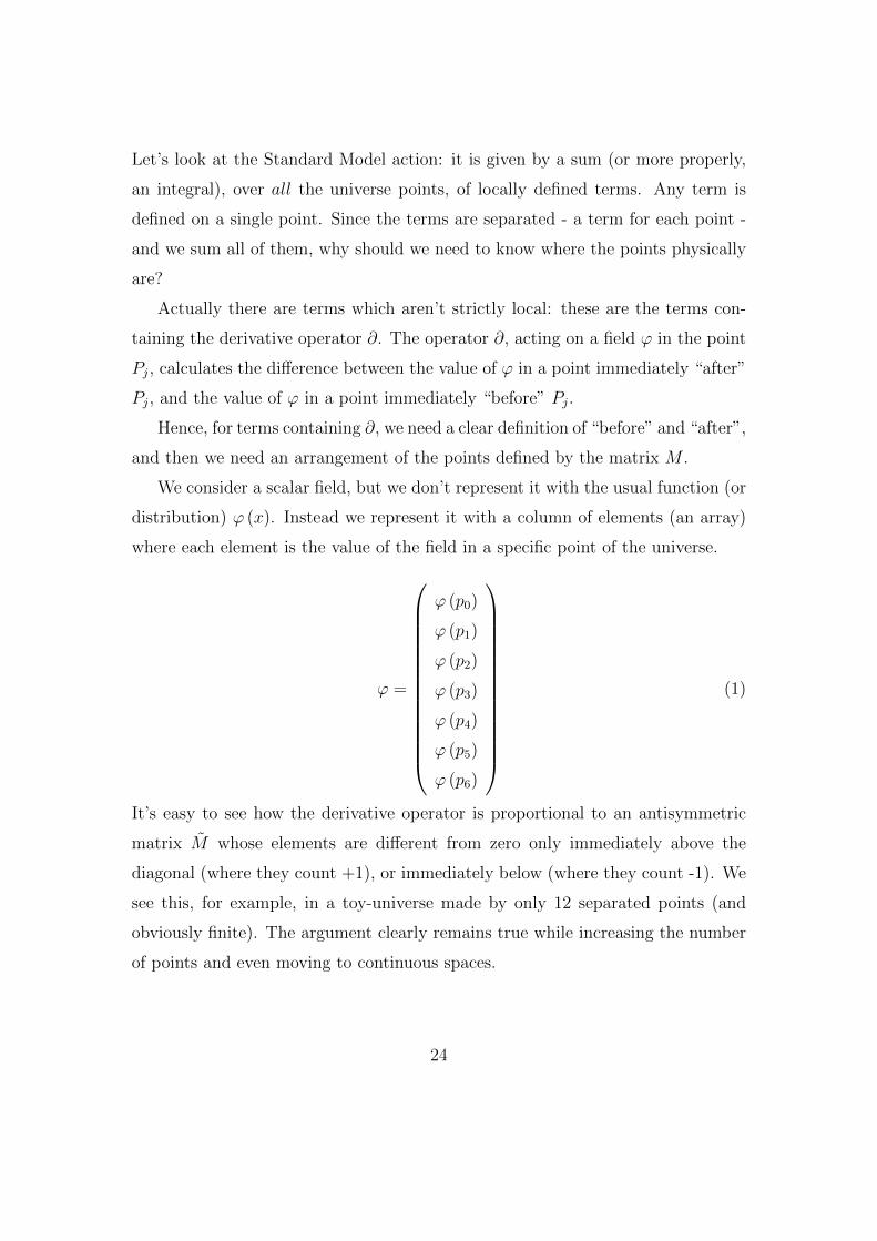
We consider a scalar field, but we don’t represent it with the usual function (or

distribution) ϕ (x). Instead we represent it with a column of elements (an array)

where each element is the value of the field in a specific point of the universe.

ϕ =

ϕ (p0)

ϕ (p1)

ϕ (p2)

ϕ (p3)

ϕ (p4)

ϕ (p5)

ϕ (p6)

(1)

It’s easy to see how the derivative operator is proportional to an antisymmetric

matrix M whose elements are different from zero only immediately above the

diagonal (where they count +1), or immediately below (where they count -1). We

see this, for example, in a toy-universe made by only 12 separated points (and

obviously finite). The argument clearly remains true while increasing the number

of points and even moving to continuous spaces.

24

∂ϕ =

0 +1 0 0 0 0 0 0 0 0 0 −1

−1 0 +1 0 0 0 0 0 0 0 0 0

0 −1 0 +1 0 0 0 0 0 0 0 0

0 0 −1 0 +1 0 0 0 0 0 0 0

0 0 0 −1 0 +1 0 0 0 0 0 0

0 0 0 0 −1 0 +1 0 0 0 0 0

0 0 0 0 0 −1 0 +1 0 0 0 0

0 0 0 0 0 0 −1 0 +1 0 0 0

0 0 0 0 0 0 0 −1 0 +1 0 0

0 0 0 0 0 0 0 0 −1 0 +1 0

0 0 0 0 0 0 0 0 0 −1 0 +1

+1 0 0 0 0 0 0 0 0 0 −1 0

ϕ (0)

ϕ (1)

ϕ (2)

ϕ (3)

ϕ (4)

ϕ (5)

ϕ (6)

ϕ (7)

ϕ (8)

ϕ (9)

ϕ (10)

ϕ (11)

(2)

=

ϕ (1)− ϕ (11)

ϕ (2)− ϕ (0)

ϕ (3)− ϕ (1)

ϕ (4)− ϕ (2)

ϕ (5)− ϕ (3)

ϕ (6)− ϕ (6)

ϕ (7)− ϕ (5)

ϕ (8)− ϕ (6)

ϕ (9)− ϕ (7)

ϕ (10)− ϕ (8)

ϕ (11)− ϕ (9)

ϕ (0)− ϕ (10)

While increasing the number of points, the (−1) still remains in the up right

corner of the matrix, and the (+1) in the down left corner as well. To eliminate

them it is sufficient to make them unnecessary, imposing boundary conditions for

25

Figure 2:

which the field is null in the first and in the last point. In fact we can describe an

open universe (a straight line), starting from a close universe (a circle) and sending

the radius to infinity. Hence we see that the conditions of null field in the first

and in the last point become the traditional boundary conditions for the Standard

Model fields.

3.3 The origin of the space-time metric

The obvious question is: is M a special entity, or is it only one of the possible

matrices M we mentioned above (connecting couple of points)?

Hence we substitute the operator ∂ in the Lagrangian with whatever matrix

M , for now antisymmetric. Acting on M with a bilinear transformation f (V,W ) :

M → M = VMW , we can always obtain the form M .

The matrices V and W combine each other in the Lagrangian to “create” a

diagonal matrix (so that Matrix (xi, xj) = 0, for i 6= j).

In this way, we can demonstrate that an action as

S =∑

µ,ν,i,j,k

M ijµ ϕ (xj)M

ikν ϕ (xk) , (3)

is equivalent to the following:

26

S =

∫dx√|h|hµν (x) ∂µϕ (x) ∂νϕ (x) (4)

where the new metric h is given by a specific combination of the matrices V and

W .

√|h|hµν (x) = Matrix (x, x) (5)

The metric h is born precisely from our attempt to arrange the space-time at all

costs. Hence the real field isn’t h but it is M .

We observe that if we accept to “see” a non-ordered universe, with M in place

of M , the metric h would’t appear and we wouldn’t measure any force of gravity.

It’s similar to what happens with centrifugal force. Let’s climb on a rotating

platform. We consider the platform stationary with respect to us. We could

describe the world around us anyway, but we should invent a new, fictitious force,

that impels things to move away from the center: it is the centrifugal force. But

if we descend from the platform, the force disappears. Accepting the chaos of the

universe is like descending from the platform. Our brain, either for an unconscious

attitude, or for genetic reasons, usually prefers by far the first option.

With this procedure, ∂ϕ = Mϕ generalizes the concept of derivative for spaces

where “a priori”arrangement of the points does not exist. We rewrite the (2) in

the integral form, extracting from M a factor 12ε

:

∂ϕ (x) =1

2ε

∫M (x, y)ϕ (y) dy (6)

M (x, y) = δ (y − (x+ ε))− δ ((y − (x− ε))) (7)

ε is the minimum coordinate distance between two points in our universe, so that

the limit ε→ 0 leads back us to the case of Hausdorff spaces. In this limit we have

that

27

1

2εM (x, y)→ −∂yδ (x− y) = ∂xδ (y − x)

So even in the continuous M maintains the antisymmetry under variables ex-

change.

3.4 The origin of entanglement and particle mass

Now, having understood what M is and how it connects to gravity, we try to

extend it. Rather than seeing it as an antisymmetric matrix, let us consider a

generic matrix. This way we’ll can include in the theory the quantum entanglement

phenomena.

If M is a generic matrix, we can always decompose it in an antisymmetric part

(which “creates” the arrangement of the space-time points and “simulates” the

derivative operator), a symmetric part with null trace (which creates the entan-

glement conditions) and a trace part (which generates the masses of the fields).

We can verify the correspondence between the trace of M and the mass of fields

in a few steps:

∂ϕ∂ϕ ∝= Mϕ·Mϕ =∑a,b,c

Mab ϕ (xa)M

cbϕ (xc) ∝

∑a,b,c

Tδabϕ (xa)Tδcbϕ (xa) = T 2

∫ϕ2

T is the trace of M , which becomes proportional to the particle mass.

In the continuous it is sufficient to substitute M with any distribution of two

variables M(x, y), replacing the sum over the indices with an integral over dy.

Mab ϕ (xa)→

∫dyM (x, y)ϕ (y) (8)

For M in the form (7), it becomes

Mab ϕ(xa)→ −

∫dy∂yδ(x− y)ϕ(y) = ∂xϕ(x) (9)

28

We consider now the symmetric component MS (x, y) = MS (y, x). A base is given

by the elements

MSB = δ (x− p) δ (y − q) + δ (x− p) δ (y − q) ,

to the vary of p and q.

In the discrete framework, posing p = point number 0 and q = point number

1, a base element is

MS =

0 1 0 0

1 0 0 0

0 0 0 0

0 0 0 0

Let’s consider the next special combination of symmetric and antisymmetric ele-

ments. We maintain p = point number 0, q = point number 1, and we add b =

point number 2.

1

2δ (x− p) δ (y − q)+1

2δ (x− q) δ (y − p)+1

2δ (x− q) δ (y − b)+1

2δ (x− b) δ (y − q)−

−1

2δ (x− p) δ (y − q)+1

2δ (x− q) δ (y − p)+1

2δ (x− q) δ (y − b)−1

2δ (x− b) δ (y − q)

= δ (x− q) δ (y − p) + δ (x− q) δ (y − b)

The symmetric elements are in the first row; the antisymmetric elements are in

the second. In the discrete framework:

1

2

0 1 0 0

1 0 1 0

0 1 0 0

0 0 0 0

+1

2

0 −1 0 0

+1 0 +1 0

0 −1 0 0

0 0 0 0

=

0 0 0 0

1 0 1 0

0 0 0 0

0 0 0 0

29

We apply the so obtained operator to the field ϕ:

0 0 0 0

1 0 1 0

0 0 0 0

0 0 0 0

ϕ (p)

ϕ (q)

ϕ (b)

ϕ (c)

=

0

ϕ (p) + ϕ (b)

0

0

Hence we see that some operators M exist, composed by symmetric and anti-

symmetric parts, which operate a real symmetrization between the points of the

space-time.

In our interpretation, the phenomena of entanglement do not break the limit

of the speed of light. In this framework the information in the first point is also in

the second point, because they are the same point. The velocity does not exceed

the speed of the light, because the covered distance is actually null. In practice,

a sort of Einstein-Rosen bridge [23] (or wormhole, 1935) is created between two

areas of the universe, and this solves the historical EPR paradox (curiously, also

published in 1935 in the same journal, Physical Review).

3.5 Measurement, Spin, Bosons, Fermions, Strings

Finally, the operator M can simulate a measurement operation, when it presents

the form:

M (x, y) = ψ (x)ψ∗ (y) (10)

→∫dyM (x, y)ϕ (y) = ψ (x)

∫dyψ∗ (y)ϕ (y) = ψ (x) (ψ, ϕ)

ψ (x) is any eigenstate, while (ψ, ϕ) denotes the scalar product between ψ and ϕ.

We can understand M as a field which determines what paths can exist:

1. continuous paths, M = −MT (fig. 3)

30

Figure 3: continuous paths, M = −MT

Figure 4: paths in entanglement, with contributes from M = MT . The matrix

symmetrizes (and so identifies) the points x3 and x4.

31

2. paths in entanglement, with contributes from M = MT . The matrix sym-

metrizes (and so identifies) the points x3 and x4. (fig. 4).

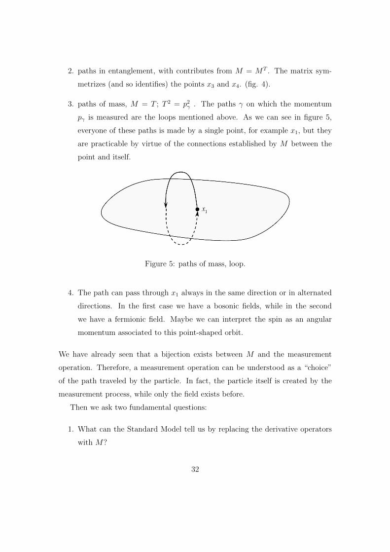
3. paths of mass, M = T ; T 2 = p2γ . The paths γ on which the momentum

pγ is measured are the loops mentioned above. As we can see in figure 5,

everyone of these paths is made by a single point, for example x1, but they

are practicable by virtue of the connections established by M between the

point and itself.

Figure 5: paths of mass, loop.

4. The path can pass through x1 always in the same direction or in alternated

directions. In the first case we have a bosonic fields, while in the second

we have a fermionic field. Maybe we can interpret the spin as an angular

momentum associated to this point-shaped orbit.

We have already seen that a bijection exists between M and the measurement

operation. Therefore, a measurement operation can be understood as a “choice”

of the path traveled by the particle. In fact, the particle itself is created by the

measurement process, while only the field exists before.

Then we ask two fundamental questions:

1. What can the Standard Model tell us by replacing the derivative operators

with M?

32

Figure 6: mass paths, loop with alternated directions.

2. Does a duality exist between our model and the String Theories? We can

see a similarity between the coordinated couple (x, y) which appears in the

non-local terms and the coordinates (σ0, σ1) on the string worldsheet. We

also trace a similarity between our model and the matrix model proposed by

Banks, Fischler, Shenker and Susskind [32]. Both our model and their one

imply the existence of a gauge group U(∞).

4 The arrangement of the space-time points

Our starting point is a physical system represented by a scalar field φ (xµ) with

(xµ) ∈ Ω ⊆ V4. Here V4 is the differential manifold space-time. As it is well

known, the dynamic evolution of the system is governed by the integral action1:

S =

∫Ω

d4x√−hL (φ, ∂φ, xµ) , (11)

where L (φ, ∂φ, xµ) is the Lagrangian density:

L (φ, ∂φ, xµ) =1

2hµν∂µφ∂νφ− V (φ) (12)

1In this paper we use natural units = c = 1.

33

In this section we aim to show that the arrangement of the space-time points is

essential only when we perform a derivation of a scalar field. For this purpose, we

develop an ad hoc mathematical formalism that will allow us to express the oper-

ation through the derivation matrix algebra. More specifically, in a 1-dimensional

model (the generalization to N dimensions is immediate) the action of the deriva-

tive operator D on the field φ is expressed through a cross product of rows and

colunms of a matrix M by a array column ϕ∞ (both infinite-dimensional). We

will see that M is an antisymmetric matrix with a particular distribution of ma-

trix elements. And they are just these last ones to “control” the arrangement of

the space-time points. In other words, passing from the matrix M to any other

antisymmetric matrix M , we can generalize the operation of derivative to space in

which an “a priori”arrangement does not exist.

4.1 1-dimensional model

Let’s start from the simplest case, a 1-dimensional space-time2. Afterwards we

shall perform an extension of the model to more dimensions. Let’s consider a

physical system, represented by a scalar field φ (x):

φ : X → R (13)

Here is X ⊆ R. We must note that the fields of physical interest are those defined

in all the space and which vanish at infinity in spatial coordinates. In the 1-

dimensional case we have a scalar field φ defined in (−∞,+∞) and such that

limx→±∞ φ (x) = 0. Assigned a > 0 we can consider the restriction of φ a Xa =

[−a, a]. Performing a equipartition Da (x−n, x−n+1, ..., xn) (see Appendix A),

the values of the field at points x−n, x−n+1, ..., xn are uniquely defined.

2Of course, the minimum dimension for space-time is formally 2 (one spatial-dimension and

one time-dimension). However, without loss of generality, it is simpler to start from a generic

1-dimensional space.

34

φk = φ (xk) , k = −n,−n+ 1, ..., n− 1, n (14)

The 2n+ 1 values taken from the field φ make up the array:

φ = (φ−n, φ−n+1, ..., φn) ∈ R2n+1 (15)

For example, for n = 3 we have the 2n+ 1 = 7 points:

x−3 = −a, x−2 = −2

3a, x−1 = −1

3a, x0 = 0, x1 =

1

3a, x2 =

2

3a, x3 = a (16)

And therefore the array:

φ = (φ−3, φ−2, φ−1, φ0, φ1, φ2, φ3) ∈ R7 (17)

It is better to consider functions from R to C, instead from R to R. Then:

φ : Xa → C

From a physical point of view only the so-called “honest” functions have a meaning,

that is, the indefinitely differentiable ones. These functions belong to the set

C∞ (Xa). As it is known, this set takes a structure of a complex vector space 3.

Introducing the scalar product:

〈φ, ψ〉 =

a∫−a

φ (x)ψ∗ (x) dx, ∀φ, ψ ∈ C∞ (Xa) , (18)

3This occurs once we have introduced the 2 operations of vector sum and product of a scalar

by a vector:

1. φ1 + φ2 | (φ1 + φ2) (x) = φ1 (x) + φ2 (x), ∀φ1, φ2 ∈ C∞ (Xa)

2. λ · φ | (λφ) (x) = λ · φ (x), ∀λ ∈ C

The element φ (x) ∈ C∞ (Xa) is a array whose infinite components are taken from the values

x ∈ [−a, a].

35

C∞ (Xa) assumes the structure of an Hilbert space. If D is the derivative operator,

then the application:

D : C∞ (Xa)→ C∞ (Xa)φ−→ dφ

dx, ∀φ∈C∞(Xa)

,

is clearly linear. That is D ∈ End (C∞ (Xa)), where the latter is the set of en-

domorphisms of C∞ (Xa). The action of the operator D is illustrated in figure

7.

Figure 7: The action of the operator D, as endomorphism that maps each element

φ of the functional space C∞ (Xa), the element dφdx

.

In other words, however we take a scalar field φ ∈ C∞ (Xa), the derivative of

this field Dφ, is still an element of the Hilbert space C∞ (Xa).

Performing an equipartition ofDa (x−n, ..., x0, ..., xn) ofXa, the array φ = (φ−n, ..., φ0, ..., φn)

stays defined belonging to the vector space C2n+1. Introducing the scalar product:

〈φ, ψ〉 =n−1∑k=−n

φkψ∗k, ∀φ, ψ ∈ C2n+1, (19)

C2n+1 assumes the structure of the Hilbert space. In the continuous the derivative

of the scalar field φ ∈ C∞ (Xa) is :

Dφ =dφ

dx=φ (x+ dx)− φ (x)

dx(20)

36

Performing an equipartition of [−a, a], the best approximation of the derivative is:

φ = (φ−n, φ−n+1..., φn) −→Dn

Dnφ =

(φ−n+1 − φ−n

∆n

,φ−n+2 − φ−n+1

∆n

, ...,φn − φn−1

∆n

),

(21)

being ∆n = xk+1−xk, the norm (or amplitude) of the partition. We note that the

formalism just developed is self-consistent, since the operation of passage to the

limit for n→ +∞ reproduces the continuous:

n−1∑k=−n

φkψ∗k −→n→+∞

a∫−a

φ (x)ψ∗ (x) dx (22)

Dnφ =

(φk+1 − φk

∆n

)k∈N\n

−→n→+∞

Dφ =

(φ (x+ dx)− φ (x)

dx

)(23)

The same limit (23) is achieved by redefining the derivative array Dnφ as follows:

Dnφ =

(φk+1 − φk−1

2∆n

)k∈N\−n,n

(24)

This is best suited for our purposes. To enumerate the components of the array

Dnφ, we consider n = 3:

φ = (φ−3, φ−2, φ−1, φ0, φ1, φ2, φ3) ∈ C7 (25)

Dn=3φ =

(φk+1 − φk−1

2∆3

)k=−2,−1,0,1,2

=

(φ−1 − φ−3

2∆3

,φ0 − φ−2

2∆3

,φ1 − φ−1

2∆3

,φ2 − φ0

2∆3

,φ3 − φ1

2∆3

)That is Dn=3φ ∈ C5, and for each n ∈ N\ 0, 1, Dnφ ∈ C2n−1, ∀φ ∈ C2n+1. The

derivative operator Dn is therefore an omomorphism between two vector spaces

C2n+1 and C2n−1, that is Dn ∈ Hom (C2n+1,C2n−1).

37

Dn : C2n+1 −→ C2n−1 (26)

φ = (φk)k∈N → Dnφ =

(φk+1 − φk−1

2∆n

)k∈N\−n,n

, ∀φ ∈ C2n−1

The vector space Hom (C2n+1,C2n−1) dimension is:

dimHom(C2n+1,C2n−1

)= dimC2n+1 · dimC2n−1 = 4n2 − 1

Let’s denote by Mn the representative matrix of the homomorphism Dn as the

canonical bases of C2n−1 and C2n+1. We note that Mn ∈ MC (2n− 1, 2n+ 1),

being the latter the vector space whose elements are the rectangular complex

matrices (2n− 1) × (2n+ 1). As we shall see in Appendix B, for n → +∞ the

MC matrices tend to become square matrices. For a → +∞, it is n → +∞, for

which the “discrete derivative” operator Dn becomes D∞; we denote by M , its

representative matrix4, shown in figure 8.

More precisely, it is:

D∞φ =1

2∆Mϕ∞ (27)

In this equation is ∆ = lima→+∞a

n(a), that is the amplitude of partition, while ϕ∞

is a column array with infinite components:

ϕ∞ =

...

φ−n

φ−n+1

...

φn−1

φn

...

(28)

4apart from the multiplicative factor 12∆ .

38

Figure 8: The matrix M . At first sight it would seem a block diagonal matrix

(with elements not being on the main diagonal). However, by highlighting the

blocks, we notice the presence of elements (+1) and (−1) between one block and

the next.

39

In summary: however we take a scalar φ ∈ C∞ (R), with the discretization just

seen, we can pass to the “discretized” field φ ∈ E∞ = limn→+∞C2n±1:

φ = limn→+∞

(φ−n, φ−n+1, ..., φn−1, φn) (29)

= (..., φ−n, φ−n+1, ..., φn−1, φn, ...) ,

whose derivative is the result of the operator of derivation D∞ ∈ End (E∞):

D∞φ =1

2∆Mϕ∞ (30)

It’s easy to accept that the k-th component D∞φ is

(D∞φ)k =1

2∆

+∞∑j=−∞

(δk,j−1 − δk,j+1)φj (31)

being δik the Kronecker delta. In fact:

(D∞φ)k =1

2∆

+∞∑j=−∞

δk,j−1φj︸ ︷︷ ︸=φk+1

−+∞∑j=−∞

δk,j+1φj︸ ︷︷ ︸=φk−1

=φk+1 − φk−1

2∆,

as it should exactly be. So the matrix elements are:

akj = δk,j−1 − δk,j+1 (32)

By performing the limit ∆→ 0, we obtain:

Dφ = Mϕ∞ (33)

Here M is a continuous matrix whose elements are:

40

a (x, x′) = lim∆→0

δ (x− (x′ −∆))− δ (x− (x′ + ∆))

2∆, (34)

while the Dφ values will be made explicit in equation (211).

The proof of these formulas is given in Appendix B.1. These results

are based on an absolute arrangement of the x axis points. More precisely, we

introduced a cartesian coordinate system R (Ox), afterwards we performed a par-

tition of a set of the type [−a, a], then performing the limit for a→ +∞, in order

to “invade” the whole R. The absolute arrangement of points directly comes from

the intrinsic arrangement of the set of real numbers R. Note, however, that from

a physical point of view, there is no reason to assign an absolute arrangement of

points. In other words, there is not an arrangement that is privileged with regards

to the others. In the formulation of physical theories the conditions of homogeneity

and isotropy of the physical space are often requested. With this new framework,

we introduce a stronger condition, eliminating the characteristics of absolute ar-

rangement of the physical space points.

To disengage the arrangement of the points, we can consider any antisymmetric

matrix M = (ajk) and consider the object:

1

2∆Mϕ∞ (35)

The (35) generalizes the notion of derivative in spaces where there is no arrange-

ment of the points in advance.

4.2 Extending the model to many dimensions

4.2.1 The Arrangement Matrix

Let’s denote by S the abstract set of the space-time points. With this term we

mean the totality of space-time points without any reference to the ordered n-

tuples of real numbers. Let’s introduce a topological structure in S (appendix C).

More precisely, we consider the discrete topology:

41

Θd = P (S) , (36)

being P (S) the set of the S parts:

P (S) = S ′ | S ′ ⊆ S (37)

So the topological space (S,Θd) is defined. With the topology (36) each subset of

S turns out to be an open set of S, referring in particular to the so-called singlets,

ie subsets of only one element: P ∈ Θd, ∀P ∈ S. As seen in Appendix C, a

base of the topological space is (S,Θd) B =PP∈S

, ie the set of all singlets.

Let’s modeling the space S so that (S,Θd) is a countable base. That means that

every open set of S is the union of a number that is, at most, countably infinite,

of singlets of the set S. Therefore:

∀A ⊆ S, ∃I ⊆ N | A =⋃i∈I

Pi (38)

This defines the surjective map:

µA : I → A, (39)

Turning out to be Pn = µA (n), with n ∈ I (fig. 9)

Definition 1 Let’s call a complete chain or a simple one, the union of the maps

µA:

µ =⋃A⊆S

µA,

with µA provided by (39).

We can represent µ as a series of “arches” that link a point of S to another,

assigning a sequence number to the points along the curve ithat is thus drawn.

42

Figure 9: Action of the surjective map µA : I → A for an arbitrary A subset of

S. The image of the I set through µA is µA (I) = A. But µA is not necessarily

injective, for which there may be points of A whose anti-image is not uniquely

defined. In the example, the point Pn′ is coming from both n′ and n′′ 6= n′.

Definition 2 Assigned N ∈ N\ 0 and A ⊆ S\ ∅, we call incomplete chain

the surjective map:

µN : N −→ A,

being N = 0, 1, ..., N.

Let us now consider two maps:

µA : I → A, νA : J → A

and the corresponding complete chains:

µ =⋃A⊆S

µA, ν =⋃A⊆S

νA, (40)

By definition of chain:

P ∈ S =⇒ ∃i, j ∈ N | µ (i) = ν (j) = P (41)

43

Furthermore:

∃k ∈ N\ i± 1 | µ (k) = ν (j + 1) (42)

Definition 3 Assigned the chains (40), we call sum of µ and ν in the P point,

the incomplete chain τ = µ+P ν:

τ : 0, 1 −→ A ⊆ S (43)

τ (0) = µ (i) = ν (j)

τ (1) = µ (k + 1)

The sum operation is illustrated graphically in figure 10.

We see that in general this sum operation is not commutative.

Figure 10: Sum of the two chains µ e ν.

Definition 4 The neutral element in the sum among chains is a pseudo-chain ∅

operationally defined by the result of the sum of chains. That is, if τ = µ+P ∅ =

∅ +P µ, with µ (i) = P , then τ (0) = µ (i) and τ (1) = µ (i+ 1). In essence, the

neutral element extracts a single bow of chain.

44

Definition 5 Assigned two incomplete chains τ e σ, such that τ (N) = σ (0), the

composition ε = τ ∪ σ is defined as:

ε (i) =

τ (i) per 0 ≤ i ≤ N

σ (i−N) per i ≥ N(44)

Basically, the operation of composition “links” the head of a chain to the tail of

another one.

Definition 6 Let’s consider a Ω set of chain containing the neutral element ∅,

Ω = ∅, µ, ν, η, ..

An incomplete chain of Ω set will correspond at Ω, whose elements are all the

possible results of the sum of the components of Ω, for all Pn points of S.

Ω = µ+P1 ∅, ν +P1 η, η +P2 µ, η +P3 ∅, ... (45)

A γ chain, external to the Ω set, it is said independent (with respect to each of the

Ω elements) if and only if is not possible to express γ through a composition of Ω

elements.

Definition 7 The S space dimensionality is the maximum number of indepen-

dent chains having S as codomain.

Definition 8 An A Field on S is an antisymmetric application from S2 to C.

A : S2 = S×A S −→ C (46)

A (Pi, Pj) = −A (Pj, Pj)

S2 is the set of all possible pairs of S points.

Consequence 9 The Arrangement Matrix M is a field on S.

45

Definition 10 For each A field and each µ chain, we define Coordinated Field

Aµ =(Aijµ)

the antisymmetric application:

Aµ = Aµ (µ× µ) : N× N −→ R (47)

Aijµ = −Ajiµ

Consequence 11 The arrangement coordinate matrix Mµ = M (µ× µ)

is a Coordinated Field on S.

4.3 Physical interpretation

4.3.1 The scalar field action in a non-ordered space-time

We extend the choice of M to the ensemble M(N) of normal matrices (MM † =

M †M), which includes (among others) the antisymmetric matrices, the symmetric

matrices, the hermitian matrices and the unitary matrices.

Given M normal matrix, an arrangement for M is a couple of matrices (D,U),

with D diagonal and U unitary, such that

DUMU † = UMU †D = 1 (48)

Theorem 12 ∀M an arrangement exists.

Proof. According to the spectral theorem ∀M ∈ M(N) ∃U unitary such that

UMU † = K with K diagonal. Setting D = K−1:

UMU †D = KD = KK−1 = 1 (49)

DUMU † = DK = K−1K = 1

CVD

46

Theorem 13 For all Mµ exists an arrangement (Dµ, U) such that the action

S =∑µ,ν

(Mµφ)(Mνφ)† + c.c

is equivalent to the standard action for a complex scalar field

S =

∫Ω

d4x∑µ,ν

√|h|hµν(x)(∂µφ

′)(∂νφ)′†

for some metrics h determined by M , with

φ′(x) = Uφ(x) (50)

φ′i(x) = φ′(xi) =

∑j

U ijφj(x) =∑j

U ijφ(xj)

Proof. As seen in (49)

UMµU†Dµ = 1 (51)

DµUMµU† = 1

We have so far assumed that U doesn’t depend on the index µ. To avoid any

misunderstanding we admit that this dependence exists and then we prove the

absurdity of this postulate. Hence

UµMµU†µDµ = 1 (52)

DµUµMµU†µ = 1

To move from M0 = Mµ=0 to M1 = Mµ=1 we apply a matrix σ01 that exchanges

the points arrangement, moving from the arrangement of chain µ = 0 to the

arrangement of chain µ = 1. The elements of σ01 are all zero except the couples

(i, j) such that (µ = 0) (i) = (µ = 1) (j). All these elements have value 1. (We

47

must no confuse the “0” in subscript with the neutral element. Here we label with

numbers from 0 to dimS the independent chains of the space S). Hence:

M1 = σ01M0σ†01

σ01σ†01 = 1 −→ σ01 ∈ U (∞)

It results:

1 = σ011σ†01 (53)

= σ01D0U0M0U†0σ†01

= σ01D0σ†01σ01U0M0U

†0σ†01

Obviously there is a choice of chains for which

[Uµ, σµν

]= 0, ∀µ, ν = 0, 1, ..., dimS (54)

The proof lies in the fact that the U (∞) generators are infinitely many, and from

these is always possible to pull out an infinite subset of commutant generators. In

this case

1 = D1U0σ01M0σ†01U

†0 = D1U1M1U

†1 (55)

We have defined D1 = σ01D0σ†01, U1 = U0. Clearly D1 is still diagonal, because

the only effect of σ01 is to change the element (i, i) with the element (j, j), when

it is (µ = 0) (i) = (µ = 1) (j).

In general we can write

1 = DµUMµU† = UMµU

†Dµ (56)

where U doesn’t depend on the chain. At this point we define:

∇µ = Mµ + Aµ, con Aµ ∈M(N) (∞,∞) (57)

48

Reasoning as we did above for M , we obtain:

1 = DµU∇µU† = U∇µU

†Dµ (58)

We explicit U∇µU†:

U∇µU† = U

(Mµ + Aµ

)U † (59)

= UU †︸︷︷︸=1

Mµ + U[Mµ, U

†]

+ UAµU†

Setting

A′µ = U[Mµ, U

†]

+ UAµU†, (60)

we obtain:

U∇µU† = Mµ + A′µ

def= ∇′µ (61)

In the continuous limit:

U∇µU† = UU †∂µ + U∂µU

† + UAµU†︸ ︷︷ ︸

=A′µ

(62)

that is:

U∇µU† = ∂µ + A′µ

def= ∇′µ (63)

Hence the transformation law for the matrix Aµ is:

Aµ →

U[Mµ, U

†]

+ UAµU†, in the “discrete”

U∂µU† + UAµU

†, in the continuous(64)

From these equations we see immediately that the matrix Aµ transforms as a gauge

field U (∞). We observe that the transformation law (64) preserves the normality

of Aµ. To view it we remember that every unitary matrix is the exponential of an

49

hermitian matrix. Hence, taking the matrix U ∈ U (∞), ∃σ ∈M(H) (∞,∞) | U =

eiσ. From this it follows:

U∂µU† = eiσ∂µ (e−iσ) = −ieiσe−iσ∂µσ = −i∂µσ

=⇒ (U∂µU†)(U∂µU

†)† = ∂µσ∂µσ† = (U∂µU

†)†(U∂µU†)

(UAµU†)†(UAµU

†) = UA†µAµU† = UAµA

†µU† =

= (UAµU†)(UAµU

†)†

=⇒ A′†µA′µ = A′µA

′†µ

=⇒ A′µ ∈M(N)(∞,∞)

Replacing the (63) into (58):

1 = D∇′µ = ∇′µD =⇒[∇′µ, D

]= 0 (65)

Taking into account the (49):

DUMµU† = D∇′µ (66)

UMµU†D = ∇′µD

Solving for Mµ:

Mµ = U †Dµ∇′µU (67)

Mµ = U †∇′µDµU

where we have redefined D as DD−1. From the comparison of these two equations,

we discover that Dµ and ∇′µ commute. At this point we explicit the summation:

∑µ,ν

(Mµφ) (Mνφ)† =∑µ,ν

(U †Dµ∇′µUφ

)(U †∇′νDνUφ

)†(68)

The terms in the summation are simply numbers (neither matrices nor arrays).

However, we can consider them as traces of matrices 1 × 1. In this sense the

previous equation can be rewritten as:

50

∑µ,ν

(Mµφ) (Mνφ)† =∑µ,ν

Tr

[(U †Dµ∇′µUφ

)(U †∇′νDνUφ

)†]In other words, Tr behaves here as the identity operator, with the additional

property of invariance respect cyclic permutations of arguments. Hence we can

rewrite:

∑µ,ν

(Mµφ) (Mνφ)† =∑µ,ν

Tr

[(U †Dµ∇′µUφ

)(U †∇′νDνUφ

)†](69)

=∑µ,ν

Tr(U †Dµ∇′µUφφ†U †∇′†νD†νU

)=∑µ,ν

Tr

(U U †︸︷︷︸

=1

Dµ∇′µUφφ†U †∇′†νD†ν

)=∑µ,ν

Tr(D†νDµ∇′µUφφ†U †∇′†ν

)=∑µ,ν

Tr(D†νDµ∇′µφ′φ′†∇′†ν

)In the last step we have taken in account the definition (50). Finally:

S =∑µ,ν

Tr(D†νDµ∇′µφ′φ′†∇′†ν

)+ c.c. (70)

=∑µ,ν

D†νDµ

(∇′µφ′

)(∇′νφ′)

†+ c.c.

=∑µ,ν

(D†νDµ + c.c

) (∇′µφ′

)(∇′νφ′)

†

It is remarkable that Dµ is diagonal:

Dijµ = dµ (xi) δ

ij (71)

We can set:

√|h|hµν (xi) = dµdν (xi) + c.c. (72)

51

Hence:

S =∑µ,ν

√|h|hµν(xi)

(∇′µφ′

)i (∇′νφ′)i (73)

In the continuous limit:

S =

∫Ω

d4x∑µ,ν

√|h|hµν (x)

(∇′µφ′

)(∇′νφ′)

†(74)

Due to the just proved theorem, we have obtained the “standard” action, with

symmetry U (∞). In addition, a metric h has appeared from nowhere.

Observation 14 We get the “impression” that the metric does not exist “a pri-

ori”, but is generated by the matrices D. In other words: The metric is simply

the result of our desire to see an ordered universe at any cost.

We focus on the relationship:

√|h|hµν (xi) = dµdν (xi) + c.c. (75)

We set:

d =

d0 + ie0

d1 + ie1

d2 + ie2

d3 + ie3

(76)

√|h|h−1 = 2

d2

0 + e20 d0d1 + e1e0 d0d2 + e2e0 d0d3 + e3e0

d0d1 + e1e0 d21 + e2

1 d1d2 + e2e1 d1d3 + e3e1

d0d2 + e2e0 d1d2 + e2e1 d22 + e2

2 d2d3 + e3e2

d0d3 + e3e0 d1d3 + e3e1 d2d3 + e3e2 d23 + e2

3

52

There are 8 independent metric components: this means that our formalism auto-

matically imposes 2 gauge conditions on the metric. In this way, the metric passes

from 10 to 8 independent components.

What other terms can we add to our action to maintain invariance for U (∞)

? Certainly the simplest is:

SHE = − i2

∑µ,ν

Tr[Mµ,M

†ν

]+ c.c. (77)

= − i2

∑µ,ν

Tr[U †Dµ∇′µU , U †∇′†νD†νU

]+ c.c. (78)

= − i2

∑µ,ν

Tr[Dµ∇′µ,∇′†νD†ν

]+ c.c.

=1

2

∑µ,ν,i

Eµν(xi)[∇′µ,∇′†ν

]iicontinuous−→ 1

2

∫d4x

∑µν

Eµν(x)[∇′µ,∇′†ν

],

where:

Eµν = −i(dµdν − dν dµ

)(79)

E = 2

0 e0d1 − e1d0 e0d2 − e2d0 e0d3 − e3d0

− (e0d1 − e1d0) 0 e1d2 − e2d1 e1d3 − e3d1

− (e0d2 − e2d0) − (e1d2 − e2d1) 0 e2d3 − e3d2

− (e0d3 − e3d0) − (e1d2 − e2d1) − (e2d3 − e3d2) 0

This term formally resembles the Einstein-Hilbert action (also the field E can be

expressed as a function of the metric h). Unfortunately, as we will see at the end of

section 4.3.3, the match is not exact. However, we will be able to find an extension

of this term which includes the Einstein-Hilbert action within.

53

4.3.2 Quantization of the field M

We expand the field M :

Mµ = Mµ + δMµ −→continuous

Mµ = ∂µ + δMµ (80)

The term (79) becomes

∂µδMν − ∂νδMµ + [δMµ, δMν ] (81)

So we have a quadratic term of “mass” and two superficial terms. These last

become null for appropriate boundary conditions on the field.

We lack a kinetic term for M . How can we build it? One option is as follows:

SGB = −∑µ,ν,α,β

[Mµ,M

†ν

] [Mα,M

†β

]+ c.c. (82)

= −∑µ,ν,α,β

[U †Dµ∇µU, U

†∇†νD†νU] [U †Dα∇αU , U

†∇†βD†βU]

+ c.c.

= −∑µ,ν,α,β

[Dµ∇µ,∇†νD†ν

] [Dα∇α,∇†βD

†β

]+ c.c.

= −∑µ,ν,α,β

(DµD

†νDαD

†β

) [∇µ,∇†ν

] [∇α,∇†β

]+ c.c.

= −∑µ,ν,α,β

(DµD

†νDαD

†β + c.c.

) [∇µ,∇†ν

] [∇α,∇†β

]= −

∑µ,ν,α,β

(hhµαhνβ + EµνEαβ

) [∇µ,∇†ν

] [∇α,∇†β

]The trouble with this term is that it generates a factor (−h) instead of

√−h.

However, we can solve the problem imposing an additional gauge condition (we

can do it because there are 4 available conditions and we have used only 2). The

condition is clearly h = −1.

The (82) could be equivalent to the classical Gauss-Bonnet term, but this must

be demonstrated. It generates terms of the following form:

54

(∂δM) (∂δM) −→ Kinetic (83)

(δM)2 (∂δM) −→ Mixed

(δM)4 −→ Potential

The potential term combines with the mass term to generate a non-trivial potential

of the form

(δM)4 − (δM)2 (84)

It has non trivial minimums that could correspond to the Einstein equation so-

lutions. It is also clear that the minimums of the potential break the symmetry

U (∞) and provide a mass to the gauge field Aµ. To view it is sufficient to rewrite

(82) as a function of Aµ and look at the quartic term:

hµαAµAαhνβAνAβ (85)

For a minimum of M there is a minimum of A, and then we perform the expansion:

Aµ = Aminµ + δAµ (86)

Therefore the (85) generates a factor:

m (x)2 hνβAνAβ (87)

m (x)2 = hµαAminµ Amin

α (88)

Hence the gauge fields acquire a mass, varying from point to point in the universe,

and essentially dependent on the metric (gravitational field). We suppose that

these masses are sufficiently large, so that the experimental physics of our day is

been unable to locate them. For the same reason, in the low energy approximation,

55

they can be omitted from the action. Neglecting the “ultra-massive”fields, the

scalar field action becomes:

S =

∫Ω

d4x∑µ,ν

√|h|hµν (x) (∂µφ) (∂νφ)† (89)

Observation 15 Someone might question the possibility to quantize the field M

since the field isn’t local. Let’s see how to do it. By exploiting the invariance of

the action under U(∞) we can always use the spectral theorem to put M0 in the

diagonal form, ie

M0(xi, xj) = M0(xi)δ(xj − xi)

Furthermore holds

Mα(xi, xj) =

∫σ0α(xi, xk)M0(xk, xl)σ0α(xj, xl)dxkdxl α = 1, 2, 3

where

σ0α(xi, xk) = δ(xm − xk) = δ(xi − xn)

(µ = α)(i) = (µ = 0)(m)

(µ = α)(n) = (µ = 0)(k)

In the same manner

σ0α(xj, xl) = δ(xp − xl) = δ(xj − xq)

(µ = α)(j) = (µ = 0)(p)

(µ = α)(q) = (µ = 0)(l)

Then:

Mα(xi, xj) = M0(xm, xp) = M0(xm)δ(xp − xm)

56

At this point, to quantize M is sufficient to quantize the local field M(x).

Let’s note that if M0 is antisymmetric, we can apply an orthogonal transfor-

mation in R(∞) ⊂ U(∞): M0 → RM0RT . In this way we can obtain a matrix M

made of blocks (2× 2) disposed on the diagonal. A similar matrix can be expanded

as follows:

M0 = M0 + δM0continuous−→ ∂0 + δM0

In this case δM0 is non zero only just above or just below the diagonal. This permit

us to describe it as the sum of two local field. Then we obtain the Mµ applying the

matrices σ0µ.

4.3.3 A final hypothesis: quantization of field M substitutes gravity

quantization

We imagine that the symmetry breaking of the group U (∞) isn’t complete, but

instead remains a residual symmetry for transformations in U (2). This means that

2 points x1, x2 exist such that the fields A(xi, xj) have null mass for i, j = 1, 2.

Then we take the term which gives masses into (SGB, eq. 82) and for simplicity

we work in the discrete framework:

SGB =∑i

LGB(xi)

LGB =∑αβγδ

[hαβ(xi)hγδ(xi) + Eαγ(xi)E

βδ(xi)]· (90)

·∞∑

m=−∞

[Aα, A†γ]xi,xm [Aβ, A

†δ]xm,xi + cinetici

[Aα, Aγ]xi,xm def

=∞∑

l=−∞

[Aα(xi, xl)Aγ(xl, xm)− Aγ(xi, xl)Aα(xl, xm)]

57

The expression (90) contains the following mass terms for the fields A(xi, xj) with

i, j = 1, 2:

Lm = m2ij

∑αβ

hαβ(xi)Aα(xi, xj)Aβ(xj, xi) i, j = 1, 2 (91)

m2ij =

∑m 6=1,2

∑γδ

hγδ(xi)Aminγ (xj, xm)Aminδ (xm, xi)

In presence of a residual symmetry for U(2) it must holds Lm = 0 and mij = 0 for

i, j = 1, 2.

It’s possible to regroup N points into N/2 ensembles Ua, with a = 1, 2, ..., N/2.

Ua ≡ Ua (xa1, xa2) (92)

In this case we can expect an extension of U (2) to U (2)N/2. This means:

Lm = m2k

∑αβ

hαβ(xa)Akα(xa)Ak′

β (xa)T kT k′

= m2k

∑αβ

hαβ(xa)Akα(xa)Ak′

β (xa) · 1

2T k, T k′

= m2k

∑αβ

hαβ(xa)Akα(xa)Ak′

β (xa)δkk′

= m2k

∑αβ

hαβ(xa)Akα(xa)Akβ(xa)!

= 0 ∀a (93)

T k are the generators of U (2) expressible in terms of Pauli’s matrices as T k = i2σk.

Furthermore:

58

Ak (xa) =i

2

∑ij

(σk)ijA(xai , x

aj

)=i

2Tr (σk · A)

m2k(x

a) =∑b 6=a,m

∑γδ

hγδ(xa)εkijAminγ (xaj , xbm)Aminδ (xbm, x

ai )

h (xa) = h (xai ) ∀i = 1, 2 (94)

E (xa) = E (xai ) ∀i = 1, 2

It is guaranteed that h (xa1) = h (xa2) e E (xa1) = E (xa2) from the invariance under

transformations in U (2), implicit in the definitions of h and E. At this point we

can consider the ensembles Ua as the “real points” of the universe, calling them

xa. Concerning the xa, symmetry is local U (2). This means that our universe

consists of 2 interchangeable sub-universes with coordinates xa1, xa2.

In this case the matricial field A (xi, xj) becomes the usual local field Ak (xa).

The same argument can be applied to U (7) imaging 7 identical sub-universes.

Why U (7)? Because this is the smallest unitary group containing the groups of

the Standard Model. In particular we suppose a symmetry breaking, with masses

of gauge field progressively decreasing, in accordance with

U(∞)→ U(7) (95)

→ SU(2)× U(5)

→ SU(2)× SU(3)× SU(2)× U(1)

→ SU(2)× SU(3)× U(1)EM

At the end of this section we will see how the first SU(2) of the sequence is sufficient

for simulating the action of the Lorentz group SO(1, 3).

Observation 16 By virtue of the definitions (94), the field of the residual gauge

SU(2) ⊂ U(2) always appear in the form:

59

Aµ = AkµTk

We remember that Aijµ (xa) = Aµ(xai , xaj ) is a normal matrix, not necessarily her-

mitian5, and so it can’t correspond to a physical quantity (a measurable field).

Nevertheless we can write:

Aµ = Bµ + iCµ

with B and C hermitian matrices. In this way, projecting the field on the genera-

tors T k, we obtain

Akµ = Bkµ + iCk

µ

Hence we can define the field

Aµ =

B1µ

B2µ

B3µ

C1µ

C2µ

C3µ

(96)

and the generators

5We could have set our model withM hermitian, from which we could have obtained hermitian

A fields. In this way we got a matrix D real, which would not have had enough degrees of freedom

to generate the metric h.

60

T =i

2

σ1

σ2

σ3

iσ1

iσ2

iσ3

(97)

with∑

k AkT k =

∑k A

kT k. The field A is an hermitian gauge field for the complex-

ification of SU(2), that we denote with SU(2)C. SU(2)C is the universal covering

group of the Lorentz group. So that’s how this group is able to appear although it

is not a unitary group in the usual sense.

As seen so far, and as we shall see shortly, the arrangement field M includes

in itself the gravitational field, a gauge field U (∞), the Higgs field and an entan-

glement field, and it behaves as a measuring observer (simulating consciousness).

It’s also remarkable that the gauge fields and the gravitational fields in our

model have different origins, although they are both born from M . The gravita-

tional field in fact appears as a multiplicative factor for moving from M to the

covariant derivative ∇. The gauge fields are instead some additive factors into

∇. For this reason we can’t quantize the gravitational field. Quantizing the gauge

fields is equivalent to quantize a piece of M in a flat space, but a similar equivalence

doesn’t exist for the gravitational field. In our framework this creates no prob-

lems, because we will quantize M directly, rather than the various gravitational

and gauge fields.

We resume now the (77) and for simplicity we consider a residual gauge for

SO(4), which substitutes SO(1, 3) in the euclidean spaces:

SHE =∑a

Eµν(xa)∑

i=0,1,2,3

∂µωiiν − ∂νωiiµ + [ωµ, ων ]ii

61

The ωijµ (xa) = ωµ(xai , xaj ) are the gauge fields SO (4). To ensure that (77) corre-

sponds to the action of General Relativity, it would be instead:

∑µ,ν,a,i,j

Rµνij (xa) · ∂µωijν − ∂νωijµ + [ωµ, ων ]

ij (98)

Rµνij =

∑ρ,σ,k,l

εµνρσεijklekρelσ (99)

The eiρ defines the tetrad, with hρσ =∑

i eiρeiσ. We see that it isn’t possible to

set Eµν = Rµνij because in the first term the indices i, j is missing. Hence it will

be necessary to modify the term (77) to obtain a tensor Eµνij . A possibility is the

following. We transform the (77) into

SHE = − i2

∑µν

Tr Z(M)[Mµ,M†ν ]

Let U(m) be the largest unitary group such that UMU † = M for U ∈ U(m)N/m.

By varying m and thus M we define a matricial function Z(M) such that Z is an

hermitian matrix ∞×∞ made of blocks, with dimension of blocks m×m.

In place of Eµν(xi) we obtain Rµν(xi, xj) = iDµZDν + c.c. which is still a

matrix made of blocks m ×m. By using the usual grouping for the coordinates,

Ua = xa1, . . . , xam:

Rµν(xi, xj)|i,j=−∞,...,∞ ⇒ Rµνij (xa)|a=1,...,N/m

i,j=1,...,m

a identify the block; i, j identifies the coordinates within the block. For m = 4 we

can obtain the Hilbert-Einstein action choosing Z(M) such that

Rµνij =

∑ρ,σ,k,l

εµνρσεijklekρelσ.

4.3.4 Superimposition

In the previous section we have seen that the “real points” for a universe with

N points and symmetry U(2) are the ensembles Ua = Ua (xai ), with i = 1, 2 and

62

a = 1, 2, ..., N/2. Under this view the scalar field decomposes as

φ (xa) =

ϕ (xa1)

ϕ (xa2)

=

1φ (xa)

2φ (xa)

(100)

The elements of SU (2) ⊂ U (2) can be interpreted as rotations in a fictitious tridi-

mensional space. Due to the particular form of the electromagnetic interaction,

in presence of a magnetic field, the fictitious rotations generate real (measurable)

magnetic moments, directed along the coordinate axes of the tridimensional space.

In this way a natural correspondence between generators and real coordinates

arises: between T 1 and x, T 2 and y, T 3 and z.

The generator of the fictitious rotation with respect the axis “i” is then propor-

tional to Si , the i-th component of the spin operator. For example, the operator

S3 results:

S3.=

2

1 0

0 −1

= −iT (3), (101)

where:

T (3) =i

2

1 0

0 −1

(102)

Calculating the normalized eigenvectors of the matrix T (3) we know the eigenstates

of the observable S3:

|↑〉 = eiφ

1

0

, with eigenvalue λ1 = +1

2(in unit = 1) (103)

|↓〉 = eiφ

0

1

, with eigenvalue λ2 = −1

2(104)

where φ is an arbitrary phase.

63

To be clear, we write the eigenvalue equation (in units = 1) for the operator

S3:

S3 |↑〉 = λ1 |↑〉 (105)

S3 |↓〉 = λ2 |↓〉

The eigenspaces are then well defined:

E (λ1) = L (|↑〉) = c↑ |↑〉 | c↑ ∈ C (106)

E (λ2) = L (|↓〉) = c↓ |↓〉 | c↓ ∈ C

From (106) we see that dimE (λk) = 1, for k = 1, 2 and, using a well-known

theorem:

C2 =3⊕

k=1

E (λk) (107)

The (107) defines the projectors:

π+ : C2 → E (λ1) (108)

π− : C2 → E (λ2)

The field φ of (100) decomposes in:

φ (x) =1 φ (x) | ↑〉+2 φ (x) | ↓〉 (109)

The projectors on the single eigenstates of S3 are

π+ =1

2

1 0

0 0

, (110)

64

π− =1

2

0 0

0 1

(111)

We see that π± are idempotent, while π+π− = 0, as it should be. A rotation by

an angle θ around the axe 1 is represented by the unitary matrix:

U1 (θ) =

cos(θ/2) −i sin(θ/2)

−i sin(θ/2) cos(θ/2)

(112)

In the special case of a rotation by π:

U1 (π) =

0 −i−i 0

(113)

We suppose now that the system is in the eigenstate |↑〉; following a rotation

around the axis 1 the state will be:

|↑〉R = U1(θ) |↑〉 ,

For θ = π:

|↑〉R = U1 (π) |↑〉 = −i |↓〉 = e−iπ/2 |↓〉 → |↓〉 , (114)

|↓〉R = U1 (π) |↓〉 = −i |↑〉 = e−iπ/2 |↑〉 → |↑〉 , (115)

since the state is defined up to an inessential phase factor. We observe that a

rotation by π around the axis 1 is equivalent to exchange “up” with “down”. This

implies the exchange of |↑〉 with |↓〉, as we have just verified by the (114) and the

(115).

The extraction of an index i from φ (x) (eq. (100)) corresponds to the extraction

of a couple of indices (i, i′) from M (x, x′) which factorizes in:

M (xi, x′i′) = M ii′ (x, x′) = M (x, x′)Rii′ , (116)

65

In the discrete framework the previous equation becomes:

M(xai , x

bj

)= M ij

(xa, xb

)= M

(xa, xb

)Rij = MabRij (117)

In both equations R is a generic matrix that in some cases can be a rotational ma-

trix. The factor Rii′ determines uniquely the result of a spin measure, exchanging

the states |↑〉 - |↓〉. This seems to suggest an identification between the arrange-

ment field M and the consciousness of an observer who performs the measurement.

5 Antisymmetric, symmetric and trace compo-

nents

We resume our initial action:

S =∑µ,ν

(Mµϕ) (Mνϕ)† = ϕ+

(∑ν

Mν

)†(∑µ

Mµ

)ϕ (118)

We note that

Λ =∑ν

Mν = M0 +M1 +M2 +M3 (119)

= M0 + σ01M0σT01 + σ02M0σ

T02 + σ03M0σ

T03

Hence an invertible matrix Θ exists such that:

Λ = ΘM0ΘT (120)

Since Θ is an invertible matrix, we could think that the only real physical entity

is Λ and M0 is simply the result of Θ−1ΛΘ−T?= ΘTΛΘ.

Hence the action can be written as:

S = ϕ†Λ†Λϕ = ϕ†Ψϕ, (121)

66

with Ψ = Λ†Λ. At this point we even wonder if Ψ is the real “physical entity”. If

we start with a real and antisymmetric Λ, then Ψ will be real and symmetric.

Given Ψ real and symmetric, two possible real solutions exist for Λ such that

Λ†Λ = Ψ. A solution returns an antisymmetric Λ, but another solution exists with

symmetric Λ. These features are reflected in two different solutions for M , so that

the action is equivalently:

S =∑µ,ν

(M (A)

µ ϕ) (M (A)

ν ϕ)†

(122)

otherwise:

S =∑µ,ν

(M (S)

µ ϕ) (M (S)

ν ϕ)†

(123)

What would be the effects of a symmetric arrangement matrix M (S)?

***

Without loss of generality, we consider the 1-dimensional case. Any matrix M∞

can be decomposed into the sum of an antisymmetric term, a symmetric term with

diagonal elements equal to zero and a trace term:

M∞ = M (A)∞ +M (S)

∞ +M (τ)∞ (124)

As we have seen, the antisymmetric component generalizes the derivative opera-

tion. We are interested in finding matrices (and therefore operators) that “sym-

metrize” distinct points of space-time. This will allow us to reinterpret the quan-

tum entanglement phenomenon.

Γ is a matrix which exchanges the points xk e xk′ .

67

Γ(kk′) def=

k k′

. . . . . . . . . . . . . . . . . . . . . . . .

k . . . 0 0 . . . 0 1 0 . . .

. . . 0 0 . . . 0 0 0 . . .

. . . . . . . . . . . . . . . . . . . . . . . .

. . . 0 0 . . . 0 0 0 . . .

k′ . . . 1 0 . . . 0 0 0 . . .

. . . . . . . . . . . . . . . . . . . . . . . .

(125)

We multiply this matrix by the infinite dimensional column array ϕ∞ (eq. (28)):

68

Γ(kk′)ϕ∞ =

k k′

. . . . . . . . . . . . . . . . . . . . . . . .

k . . . 0 0 . . . 0 1 0 . . .

. . . 0 0 . . . 0 0 0 . . .

. . . . . . . . . . . . . . . . . . . . . . . .

. . . 0 0 . . . 0 0 0 . . .

k′ . . . 1 0 . . . 0 0 0 . . .

. . . . . . . . . . . . . . . . . . . . . . . .

× (126)

×

. . .

k φ (xk)

0

. . .

0

k′ φ (xk′)

. . .

We obtain:

Γ(kk′)ϕ∞ =

. . .

k φ (xk′)

0

. . .

0

k′ φ (xk)

. . .

(127)

The resulting array is invariant under the exchange of k with k′ (also provided to

69

exchange their positions). Summing to the matrix Γ a trace term, we obtain the

matrix S(kk′) which symmetrizes the two points xk e xk′ :

S(kk′) =

k k′

. . . . . . . . . . . . . . . . . . . . . . . .

k . . . 0 0 . . . 0 1 0 . . .

. . . 0 0 . . . 0 0 0 . . .

. . . . . . . . . . . . . . . . . . . . . . . .

. . . 0 0 . . . 0 0 0 . . .

k′ . . . 1 0 . . . 0 0 0 . . .

. . . . . . . . . . . . . . . . . . . . . . . .

+ (128)

+

k k′

. . . . . . . . . . . . . . . . . . . . . . . .

k . . . 1 0 . . . 0 0 0 . . .

. . . 0 0 . . . 0 0 0 . . .

. . . . . . . . . . . . . . . . . . . . . . . .

. . . 0 0 . . . 0 0 0 . . .

k′ . . . 0 0 . . . 0 1 0 . . .

. . . . . . . . . . . . . . . . . . . . . . . .

Hence:

70

S(kk′) =

k k′

. . . . . . . . . . . . . . . . . . . . . . . .

k . . . 1 0 . . . 0 1 0 . . .

. . . 0 0 . . . 0 0 0 . . .

. . . . . . . . . . . . . . . . . . . . . . . .

. . . 0 0 . . . 0 0 0 . . .

k′ . . . 1 0 . . . 0 1 0 . . .

. . . . . . . . . . . . . . . . . . . . . . . .

(129)

Running the product S(kk′) · ϕ∞ we obtain:

S(kk′)ϕ∞ =

. . .

k φ (xk) + φ (xk′)

0

. . .

0

k′ φ (xk) + φ (xk′)

. . .

(130)

Hence the resulting array is invariant under the exchange of the coordinates xk

and xk′ .

In the same way we define the matrix Γ[kk′] which anti-exchanges the points xk

e xk′ :

71

Γ[kk′] def=

k k′

. . . . . . . . . . . . . . . . . . . . . . . .

k . . . 0 0 . . . 0 1 0 . . .

. . . 0 0 . . . 0 0 0 . . .

. . . . . . . . . . . . . . . . . . . . . . . .

. . . 0 0 . . . 0 0 0 . . .

k′ . . . −1 0 . . . 0 0 0 . . .

. . . . . . . . . . . . . . . . . . . . . . . .

(131)

We multiply this matrix by ϕ∞:

Γ[kk′]ϕ∞ =

. . .

k φ (xk′)

0

. . .

0

k′ −φ (xk)

. . .

(132)

The resulting array reverses its sign for the exchange of k with k′ (also provided

to exchange their positions). Summing to the matrix Γ a trace term, we obtain a

matrix S[kk′] which anti-symmetrizes the two points xk and xk′ :

72

S[kk′] =

k k′

. . . . . . . . . . . . . . . . . . . . . . . .

k . . . 0 0 . . . 0 1 0 . . .

. . . 0 0 . . . 0 0 0 . . .

. . . . . . . . . . . . . . . . . . . . . . . .

. . . 0 0 . . . 0 0 0 . . .

k′ . . . −1 0 . . . 0 0 0 . . .

. . . . . . . . . . . . . . . . . . . . . . . .

+ (133)

+

k k′

. . . . . . . . . . . . . . . . . . . . . . . .

k . . . −1 0 . . . 0 0 0 . . .

. . . 0 0 . . . 0 0 0 . . .

. . . . . . . . . . . . . . . . . . . . . . . .

. . . 0 0 . . . 0 0 0 . . .

k′ . . . 0 0 . . . 0 1 0 . . .

. . . . . . . . . . . . . . . . . . . . . . . .

Hence:

73

S[kk′] =

k k′

. . . . . . . . . . . . . . . . . . . . . . . .

k . . . −1 0 . . . 0 1 0 . . .

. . . 0 0 . . . 0 0 0 . . .

. . . . . . . . . . . . . . . . . . . . . . . .

. . . 0 0 . . . 0 0 0 . . .

k′ . . . −1 0 . . . 0 1 0 . . .

. . . . . . . . . . . . . . . . . . . . . . . .

(134)

As usual, multiplying S[kk′]ϕ∞ we find:

S[kk′]ϕ∞ =

. . .

k φ (xk)− φ (xk′)

0

. . .

0

k′ φ (xk)− φ (xk′)

. . .

(135)

Hence the resulting array reverses its sign under the exchange of the coordinates

xk and xk′ .

We immediately verify the following relations:

S[kk′] · Γ(kk′) · S[kk′] = 0 (136)

S(kk′) · Γ[kk′] · S(kk′) = 0

S[kk′] · S(kk′) = 0

74

Furthermore, we derive:

(Γ(kk′)φ

)i

= δikφ (xk′) + δik′φ (xk) (137)(Γ[kk′]φ

)i

= δikφ (xk′)− δik′φ (xk)(S(kk′)φ

)i

= (δik + δik′) [φ (xk′) + φ (xk)](S[kk′]φ

)i

= (δik + δik′) [φ (xk′)− φ (xk)]

Now we suppose that xk and xk′ are the anti-images (by some chains µ) of two

points P and P ′ in S, separated by a macroscopic distance r (fig. 11).

Figure 11: The points P and P ′ have anti-images xk and xk′ , respectively.

For what said, we are considering two points P and P ′ such that

|xk′ − xk| = r (138)

From xk = k∆ (eq. 199, appendix A) we derive:

|xk′ − xk| = |k′ − k|∆ (139)

Hence:

|k′ − k| = r

∆(140)

This result is consistent because in the limit ∆ → 0+ is |k′ − k| → +∞. Thus

(139) assumes the indeterminate form 0 · ∞ which reduces to the macroscopic

distance 0 < r < +∞.

We rewrite the third of the (137):

75

(S(kk′)φ

)i

= (δik + δik′) [φ (xk′) + φ (xk)] (141)

Runnig to the limit ∆ → 0, the points xk and xk′ remain finitely separated.

However, between the columns k and k′ in the matrices, appears an infinite number

of columns. The same holds for the rows. Said that, in the continuous we find:

(S(PP ′)φ

)(x) = [δ (x− xP ) + δ (x− xP ′)] [φ (xP ) + φ (xP ′)] (142)

5.1 Commutation relations. Bosonic and fermionic fields

We rewrite the (137):(Γ(kk′)φ

)i

= δikφ (xk′) + δik′φ (xk) (143)(Γ[kk′]φ

)i

= δikφ (xk′)− δik′φ (xk)(S(kk′)φ

)i

= (δik + δik′) [φ (xk′) + φ (xk)](S[kk′]φ

)i

= (δik + δik′) [φ (xk′)− φ (xk)]

In the continuous limit they become:

(Γ(PP ′)φ

)(x) = δ (x− xP )φ (xP ′) + δ (x− xP ′)φ (xP ) (144)(

Γ[PP ′]φ)

(x) = δ (x− xP )φ (xP ′) + δ (x− xP ′)φ (xP )(S(PP ′)φ

)(x) = [δ (x− xP ) + δ (x− xP ′)] [φ (xP ) + φ (xP ′)](

S[PP ′]φ)

(x) = [δ (x− xP ) + δ (x− xP ′)] [φ (xP )− φ (xP ′)]

In the continuous the (136) become:

S[PP ′] · Γ(PP ′) · S[PP ′] = 0 (145)

S(PP ′) · Γ[PP ′] · S(PP ′) = 0

S[PP ′] · S(PP ′) = 0

76

Proposition 17 If we choose the scalar fields φ1 (x), φ2 (x), we can express the

relationship of commutation (or anti-commutation) in terms of Γ(PP ′) (or Γ[PP ′]):

[φ1 (x) , φ2 (x)] = φ1 (x) Γ[PP ′]φ2 (x) (146)

φ1 (x) , φ2 (x) = φ1 (x) Γ(PP ′)φ2 (x)

Proof. We work in the discrete framework. Then we’ll run the limit ∆ → 0.

From the second of the (137) we get:

φ1 (xi) Γ[kk′]φ2 (xi) = φ1 (xi) [δikφ2 (xk′)− δik′φ2 (xk)] (147)

= φ1 (xi) δikφ2 (xk′)− φ1 (xi) δik′φ2 (xk)

= φ1 (xk)φ2 (xk′)− φ1 (xk′)φ2 (xk)

In the same manner we can demonstrate the second of the (146).

Accordingly, we consider a bosonic field consisting of only two “particles“localized

in xP and xP ′ respectively. It’s obvious that:

φB (x) = S(PP ′)φ (x) (148)

In the discrete framework we can apply the first of the (146):

[φB (xk) , φB (xk′)] = φB (xi) Γ[kk′]φB (xi) (149)

=(S(kk′)φ (xi)

)T· Γ[kk′] · S(kk′)φ (xi)

= φ (xi)T(S(kk′)

)T· Γ[kk′] · S(kk′)φ (xi) = 0

In the last step we took into account the (136). The result (149) has an obvious

generalization in the continuous.

We consider now a fermionic field consisting of only two “particles”localized in

xP and xP ′ respectively. It’s obvious that:

77

φF (x) = S[PP ′]φ (x) (150)

Proceeding in the same manner, we find:

[φF (xk) , φF (xk′)] = φ (xi)T(S[kk′]

)T· Γ(kk′) · S[kk′]φ (xi) = 0

We have so obtained the usual rules of commutation and anti-commutation, with-

out the need to introduce Grassmann variables.

The reasoning can be extended to an infinite number of particles, even contin-

uous, in order to consider the usual bosonic and fermionic fields used in QFT.

We consider that it is possible to describe fermion fields simply factorizing a

factor S[kk′] from M . We wonder if we can also obtain the usual fermionic action

from terms of the form (77) or (82) as we do with gauge fields. Garrett Lisi has

already shown [33] how the fermionic fields can transform as gauge fields provided

we enlarge the usual unitary groups SU (k) to specific exceptional Lie groups.

5.2 Fermionic action

What follows, until the end of this sub-section, has to be taken as notes, since

much remains to be verified. We have some ideas for constructing a fermionic

action. We imagine that the existence of a superimposition of universes descends

from the existence of some extra-dimensions. These dimensions can be fermionic

dimensions with anticommutation rules for the coordinates.

We indicate with QA the usual generators of the translations in the fermionic

dimensions. The capital letters indicate coordinates in these dimensions (θA). The

QA are the equivalent of the derivatives in the usual space-time. You can find a

good description of QA in [34].

QA =

Qα

Qα

θA =

θα

θα

78

Qα = ∂α − i(σµ)ααθα∂µ

Qα = −∂α + i(σµ)ααθα∂µ

As ∂ can be extended to ∇, the Q can be extended to

Qα = ∂α − i(σµ)ααθα∇µ

Qα = −∂α + i(σµ)ααθα∇µ

Let consider that the usual fermionic action is equivalent to

SF =1

2

∫dx∑A,B

ψAQA, QBψB =

∫dx iψ†γ0γµ∇µψ

We have preferred to write explicitly ψ†γ0 instead of ψ = ψ†γ0 as we find in the

standard treatments on fermions. This is to avoid confusion because, in the rest

of the article, the scripture ψ simply indicates complex conjugation. The above

result follows from

QA, QB = 2i (Cγ)µAB ∂µ

or

QA, QB = 2i (Cγ)µAB∇µ

in the extended version. C is the charge conjugation operator.

Obviously we can write the QA in the form of matrices, in the same way we

have done with ∇ in the bosonic case. Once we have done it, we can write:

SF =1

2Tr∑A,B

(ψBψA)QA, QB =1

4Tr∑A,B

[ψB, ψA]QA, QB

where we have used the cyclic invariance of the trace and

2ψAψB = ψAψB + ψAψB = ψAψB − ψBψA = [ψA, ψB]

79

Actually, this matrical product is equivalent to

SF =1

4Tr∑A,B

[QA + ψA, QB + ψB]QC + ψC , QD + ψDδACδBD

This is because QAQC is antisymmetric on A ↔ C. So it’s zero when it is con-

tracted with δ. Moreover ψC , ψD = 0. In these way the fermionic field ψ

composes with Q a covariant derivative, acting as a gauge field. As shown by Gar-

rett Lisi [33], the fundamental representation for the unitary groups corresponds

to the adjoint representation in the exceptional groups which include the unitary

ones. A gauge field have to transform in the adjoint representation, so these can be

covariant derivatives only for an exceptional Lie group. For example, the adjoint

representation for the exceptional group G2 is

g2 = su(3) + 3 + 3

where su(3) is the adjoint representation for SU(3) describing gluons, 3 is the

fundamental representation describing quark (red, green, blue) and 3 is its dual,

describing anti-quark. However, for every exceptional Lie group, another unitary

group exists which includes it. For example G2 ⊂ SO(7) ⊂ U(7)

What we suggest is that the fermionic action derives from a Gauss-Bonnet type

term, as

SGB =1

4Tr

∑A,B,C,D

[M †A,MB]M †

C ,MD.

The masses will arise from non-null expectation values in the usual fields Aµ, which

are contained in ∇.

80

6 Quantum Entanglement

6.1 Bohm interpretation

In this section we treat the quantum entanglement phenomena (Verschrankungof

[25], definition by Schrodinger, 1935) within the framework developed in the pre-

ceding sections. In particular, we see that the symmetric component of the matrix

M∞ enables us to reinterpret these phenomena.

For this purpose we start from the description elaborated in 1951 by David Bohm

6 [27], [35].

Let’s consider a system composed of two spin-12

particles (denoted by 1 and 2).

The total spin angular momentum is:

~S = ~S1 + ~S2

In operatorial terms:

~S = ~S1 + ~S2, (151)

If the composite system is in the singlet-spin state s = 0, mS = 0, then the state

spin vector is:

|s = 0,mS = 0〉 =1√2

(|+−〉 − |−+〉) , (152)

where:

S1z |+−〉 =2|+−〉

S2z |+−〉 = −2|+−〉

etc.

6Specifically, we follow the exposition presented by Sakurai [35] in 1985.

81

From (152) we deduce that, performing a measurement of the Sz spin component

of single particle, we have a probability equal to 12

to find |+〉 or |−〉. However,

if we find particle 1 in the spin state “up” |+〉, a subsequent measurement of the

same spin component of particle 2 will necessarily result in the spin state “down”

|−〉. In other words, there is a correlation between the same spin components of

the two particles, so that s = 0. Incidentally, this correlation remains as such even

when the two particles are separated by a macroscopic distance. The separation

may occur through a spontaneous disintegration of the system into its spin 12

components. Such a system could be, for example, the result of the proton-proton

diffusion at low energies. For the Pauli exclusion principle, the two interacting

protons lie in the singlet-spin state, while the orbital angular momentum is equal

to 0. For this system, therefore, an equation of type (152) is valid. Taking into

account the orbital degrees of freedom, the system state ket (in the appropriate

Hilbert space) is:

|Ψ〉 = |φ〉 ⊗ |s,ms〉 ≡ |φ〉 |s,ms〉 (153)

In the position representation the wave function is:

Ψ (x1,x2, ~σ) = 〈x1,x2|Ψ〉 = φ (x1,x2)ψ (~σ) , (154)

Hereby we have symbolically incorporated in ~σ the spin variables. In (154) x1,x2

are the spatial coordinates of single particle. Passing to the center-of-momentum

frame and of the relative coordinate xr = x2 − x1, the (154) becomes:

Ψ (x, ~σ) = φ (x)ψ (~σ) , (155)

having redefined xr in x. Then we observe that the spin wave function ψ (~σ) can

be written in terms of single particle spin, through the expansion of the vector

(152). Denoting symbolically by ~σ1 and ~σ2 the spin variables of single particle, we

have:

82

Ψ (x, ~σ1, ~σ2) = φ (x)ψ (~σ1, ~σ2) , (156)

Let’s assume that at initial time t0 the composite system, which is in the singlet-

spin state |s = 0,mS = 0〉, disintegrates spontaneously, for which the particles 1

and 2 move away along two opposite directions. At a time t the particles will be

separated by a macroscopic distance x′:

x = 0 at t0 (157)

x = x′ 6= 0 at t > t0

Therefore:

Ψ (0, ~σ1, ~σ2) = φ (0)ψ (~σ1, ~σ2) at t0 (158)

Ψ (x′, ~σ1, ~σ2) = φ (x′)ψ (~σ1, ~σ2) at t

In this specific example, particle 1 moves in the positive way of a ~r direction, while

particle 2 moves in the negative direction, as shown in figure 12.

In this figure, also, A e B denote two observers with their detectors (they are

symbolically represented with two small rectangles). Now let’s suppose we direct

the x axis to the positive direction of ~r axis.

In such scheme A measures S1z (spin components of the particle 1 along the z

axis), while B measures S2z, that is the spin component of particle 2 in the same

direction. For example, if A finds the particle 1 in the state |+〉, he/she will

necessarily know with certainty (probability = 1) that B will find the particle 1 in

the state |−〉, before B performs the measurement. If, however, A does not make

any measurement, B will have a probability equal to 12

to find the spin of particle 2

in up or down state. So, if B performs a measurement before A, these conclusions

are still applied even if we reverse the order in which the measurements are done.

In other words, there is a 100% correlation between the measurements made by A

83

Figure 12: Particle 1 moves in the positive direction of the ~r axis, while particle

2 moves in the opposite direction. In the figure the reference system is chosen so

that the x-axis is oriented in the direction of ~r.

and B. Let’s note that the two particles lie at a macroscopic distance x′ from each

other and therefore they can not exchange information except through a non-local

field (action-at-a-distance).

However, these results due to the rotational invariance singlet-spin state, should

not surprise us. In other words, the results obtained by B will always be opposite

to those obtained by A. In contrast, interesting results are obtained when the

components are measured along different axes. For this purpose, let’s rewrite the

(152) as follows:

|s = 0,mS = 0〉 =1√2

(|z+; z−〉 − |z−; z+〉) (159)

in which we remember that we have chosen the z axis as the direction of measure-

ment. Of course we are free to choose either the x or the y axis. For example, if

we choose the x axis, the theory of angular momentum composition says that the

singlet-spin is:

84

|s = 0,mS = 0〉 =1√2

(|x−; x+〉 − |x+; x−〉) (160)

Let’s imagine the following scenario:

A measures Sz o Sx of the particle 1.

B measures Sx of the particle 2.

If A measures Sz and finds particle 1 in the |z+〉 state (this implies with certainty

that the z axis component of the spin particle 2 is down), the observer B will have

a probability equal to 12

to find particle 2 in one of two states |x+〉 o |x−〉. If,

instead, A measures Sx and finds particle 1 in |x+〉 state, he/she will know with

certainty that the results of the measurements performed by B is |x−〉.We conclude that, for individual observers, if the axes of measurement are the

same, there will be a 100% correlation between the two measurements. Conversely,

if the axes are different, there is a random correlation. Therefore the results of

measurements performed by B seem to depend on the measurement performed by

A. In other words, it is as though there was a pre-knowledge by particle 2 on the

measurements made by A. Let’s recall also that the two particles are separated

by a macroscopic distance that can be made arbitrarily large.

6.2 Quantum Entanglement in the M field framework

To interpret the entanglement quantum phenomena in our framework, we summa-

rize in a broad outline the formalism developed. Let’s start with an abstracts S

set of points in space, equipped with a suitable topological structure. Then let’s

consider a field represented by an infinite-dimensional matrix M that, as we have

seen, decomposes into the sum of three terms (symmetric, antisymmetric, trace).

To avoid unnecessary complications, we consider the 1-dimensional case (the gen-

eralization to a higher number of dimensions is immediate). In Section 5 we saw

that7 (eq. (141)):

7The symbol S∞ denotes the symmetrization operator, not to be confused with the symbol

denoting the spin of the particle.

85

(S(kk′)φ

)i

= (δik + δik′) [φ (xk′) + φ (xk)] , (161)

Hereby S(kk′) is performed by (129), while xk and xk′ are the anti-images (by some

chains µ) of two points P and P ′ in S, separated by a macroscopic distance r (fig.

13).

Figure 13: The points P and P ′have anti-images xk and xk′, respectively.

Let’s note that xk = k∆, for which xk 6= xk′ , since it is k 6= k′. However, the

concept of distance is defined only in the ordered space, and the chain µ : Z→ S

is not a injective map. This means that xk and xk′ could be two anti-images of the

same point P = P ′!

= Q. A symmetric matrix M like S(PP ′) exactly corresponds

to a map µ which has this effect. As a formula it is:

(S(kk′)φ

)i

= (δik + δik′) [φ (xk′) + φ (xk)] =⇒ ∃Q ∈ S | k = µ−1 (Q) , k′ = µ−1 (Q)

(162)

=⇒ (xk e xk′ identify the same point Q of S

In other words, the symmetric component applied to the scalar field φ “makes”

xk and xk′ to be the same point in S space. Obviously, in the space x (where

there is an arrangement in advance) xk and xk′ identify distinct points. All this is

summarized in Figure 14.

Performing the limit for ∆→ 0:

(S(PP ′)φ

)(x) = [δ (x− xP ) + δ (x− xP ′)] [φ (xP ) + φ (xP ′)] (163)

Generalizing (163) to the 3-dimensional physical space:

86

Figure 14: k and k′ 6= k identify different “ordered” space points , but -

through the action of the matrix S(PP ′) - they identify the same point

in the space S where an arrangement in advance does not exist.

(S(PP ′)φ

)(x) =

[δ(3) (x− xP ) + δ(3) (x− xP ′)

][φ (xP ) + φ (xP ′)] (164)

Hereby the scalar field φ (x) can be the wave function of the system composed by

particles 1 and 2 (eq. 155). As said xk and xk′ identify the same point of S. It

follows that the spatial separation of the two particles is only the result

of our will to see the universe ordered at all costs. At this stage we can

say that M generates both Gravity and Entanglement. The obvious conclusion

that we can draw is that there is not a qualitative difference between two particles

in Entanglement and two Blacks Holes connected by a Einstein-Rosen bridge.

7 The trace term and the mass of the fields

Let’s recall the decomposition equation (124):

M∞ = M (A)∞ +M (S)

∞ +M (τ)∞ (165)

Denoting by M(τ)ij = miδij the generic matrix element of the term trace M

(τ)∞ , let’s

explicit the product:

87

∑i,j,k

Mijφ (xj)Mikφ (xk) =∑i

m2iφ (xi)φ (xi) −→

continuo

+∞∫−∞

m (x)2 φ (x)φ (x) dx (166)

From this equation we see that the trace of the matrix M (τ), and then the matrix

M (by virtue (165) ) generalized to continuous), is proportional to the mass of the

scalar field φ (x).

8 Measurement of a quantum observable

Let’s recall the decomposition equation (124). From this equation it follows that

for every element M∞ of the vector space MC (∞,∞), such element is decomposed

into the sum of three terms:

M∞ = M (A)∞︸ ︷︷ ︸↓

(+1) (−1)

+ M (S)∞︸ ︷︷ ︸

Entanglement

+M (τ)∞︸︷︷︸

Mass

(167)

The symbols in the second member of (167) remind us that the antisymmetric

term can be reduced to the (+1) (−1) form, the symmetric term can be reduced

to the form (129), while the trace term is proportional to the mass of the scalar

field on which it acts (see the previous section). In the continuous limit:

M∞ −→continuous

M = (M (x, x′)) , x, x′ ∈ RN (or VN N-dimensional manifold )

(168)

That said, let’s consider a quantum mechanics system Sq in non-relativistic regime.

As it is well known, the system state is described by a wave function ψ as an element

of a separable Hilbert space H [36].

Let A be an observable associated to Sq. If A is the corresponding self-adjoint

operator, we have:

88

A |ak〉 = ak |ak〉 , ak ∈ σd(A)

(169)

A |a〉 = a |a〉 , a ∈ σc(A)

The (169) are the eigenvalues equations for A, written in the bracket Dirac notation

[37]. In these formulas, σd

(A)

and σc

(A)

are respectively the discrete and the

continuous spectrum of the operator A.

Observation 18 For simplicity we are considering the non-degenerate eigenval-

ues case. For more details, see Appendix D.

As it is well known |ak〉ak∈σd(A)∪|a〉a∈σc(A) is a complete orthonormal system

in H, for which the vector state |ψ〉 is:

|ψ〉 =

N≤+∞∑k=1

ck |ak〉+

∫σc(A)

c (a) |a〉 (170)

The coefficients of the linear combination (170) are given by:

ck = 〈ak|ψ〉 (171)

c (a) = 〈a|ψ〉

Without loss of generality, let’s suppose that the spectrum of A is purely discrete,

for which σc

(A)

= ∅. So that the state vector expansion in the eigenvector of A

is:

|ψ〉 =N∑k=1

ck |ak〉 (172)

The dynamic evolution of the system is governed by the Schrodinger equation or,

that is the same, by the application of the time evolution operator U (t, t0) =

e−i H(t−t0) to the vector state (172), obtaining the system state at any time.

|ψ (t)〉 =N∑k=1

ck (t) |ak〉 (173)

89

In order not to overburden the notation we put |ψ〉 ≡ |ψ (t∗)〉, ck ≡ ck (t∗), being

t∗ the time when the measurement of the observable is performed. Then:

|ψ〉 =N∑k=1

ck |ak〉 (174)

|ψ〉 −→mis A

|an〉

In other words, following the measurement of A, the system “jumps” from the

state |ψ〉 to some eigenstate |an〉, while the probability of finding the system in

the state |an〉 (or, what is the same, of finding the value an) is:8:

P (A = an, t∗) = |cn (t∗)|2 (175)

Let Eak be the eigenspace corresponding to the eigenvalue ak, or, that is the same,

the vector subspace of H which elements are the eigenvector corresponding to the

eigenvalue ak:

Eak =|u〉 ∈ H | A |u〉 = ak |u〉

(176)

By a well-known theorem, H decomposes into the direct sum of eigenspaces (176):

H =N⊕k=1

Eak (177)

The eigenspaces Eak are orthogonal:

〈ak|ak′〉 = δkk′ =⇒ Eak⊥Eak′ 6=k

The (177) defines N projection operators Pak ∈ Hom (H, Eak):

H =N⊕k=1

Eak =⇒ ∃Pak

k∈N⊂ Hom (H, Eak) | Pak : H −→ Eak

|ψ〉−→ck|ak〉(178)

8If |ψ〉 is normalized: |||ψ〉||2 = 〈ψ|ψ〉 = 1

90

N = 1, 2, ..., N.That is:

∀ |ψ〉 ∈ H, Pak |ψ〉 = ck |ak〉 (179)

The operators Pak verify the following properties:

PakPak′ = δkk′Pak′ (180)

N∑k=1

Pak = 1

From the first formula (180) it follows that P 2ak

= Pak , i.e. the projection operators

are idempotent, and, for a known property σ(Pak

)= 0, 1. It is easy to derive

the Pak analytical expression:

Pak = |ak〉 〈ak| (181)

In fact:

PakPak′ = |ak〉 〈ak|ak′〉 〈ak′ | = δkk′ |ak〉 〈ak′ | (182)

N∑k=1

|ak〉 〈ak| = 1

We see that the measurement operation(174) is the result of applying the projec-

tion operator Pan to the vector state |ψ〉:

Pan |ψ〉 = cn |an〉 (183)

In summary: to the quantum observable A, it is associated a complete orthog-

onal system of projection operatorsPak

k∈N

that simulates a measurement.

The eigenvalues equations (169) can be written in terms of eigenfunctions. In fact,

in the position representation, the eigenfunctions of A are:

91

uk (x) = 〈x|ak〉 (184)

u (x) = 〈x|a〉 ,

for which:

Auk (x) = akuk (x) (185)

Aua (x) = aua (x)

The system wave function is ψ (x) = 〈x|ψ〉:

ψ (x) =N∑k=1

ckuk (x) +

∫σc(A)

c (a)ua (x) da (186)

From the (171) it is easy to derive the analytical expression of the expansion

coefficients into the (186):

ck =

+∞∫−∞

u∗k (x)ψ (x) dx (187)

c (a) =

+∞∫−∞

u∗a (x)ψ (x) dx

The (174) becomes:

ψ (x, t) =N∑k=1

ck (t)uk (x)

ψ (x, t∗) −→misA

un (x) , with n ∈ 1, 2, ..., N

After this long introduction, we take the matrix (168)9:

9The symbol used is the A = (aik) type. We have not indicated with m (x, x′) the generic

matrix element of M , to avoid a proliferation of symbols.

92

M = (M (x, x′)) (188)

Obviously:

∃M |M (x, x′) = un (x)u∗n (x′) , (189)

being un (x) the eigenfunction of A corresponding to the eigenvalue an. Using the

Dirac notation:

M (x, x′) = 〈x|an〉 〈an|x′〉 (190)

= 〈x| Pan |x′〉 ≡Man (x, x′)

That is, if M (x, x′) admits a factorization of the type (189), then the M (x, x′)

are the matrix elements (in the position representation) of the projection operator

Pan . But we have just seen that the projection operator simulates a measurement.

Consequence 19 The M field arrangement “is able to perform” a measurement

of a quantum observable.

Observation 20 We achieve the same result without using the Dirac notation.

For this purpose, we remember that the M matrix rappresents an endomorphism

in the vector space10 E∞ (appendix B.1).To avoid a proliferation of symbols, let’s

denote by the same symbol that endomorphism. Therefore, the result of applying

M to a scalar field φ (x) is:

Mφ (x) =

+∞∫−∞

M (x, x′)φ (x′) dx′, (191)

where the integral in the second member is the generalization to the continuous

of the product rows by columns. Let us act the M operator on the system wave

10More precisely, the E∞ generalization to the continuous.

93

function (at time t∗) , with M (x, x′) given by (189):

Mψ (x) =

+∞∫−∞

un (x)u∗n (x′)ψ (x′) dx′ (192)

= un (x)

+∞∫−∞

u∗n (x′)ψ (x′) dx′

By the first (187):

Mψ (x) = cnun (x) (193)

In the Appendix E we report further considerations accompanied by an example

of a physical system.

9 Physical consequences

9.1 Non-commutative geometry

From what it has been suggested at page 22 we can interpret M ik, in the one-

dimensional case, as the probability amplitude for the point i to be connected to

the point k. In the general case we can believe that this amplitude is expressed

by Λik. In the case of generic M or Λ, it can be |Λik|2 6= |Λki|2. This means that

i can be connected to k while k isn’t connected to i. Hence we are in presence of

a non-commutative geometry. The probability amplitude that i e k are mutually

connected (we can say “classical” connection) is:

Amp. = ΛikΛki

The probability amplitude that the point i is classically connected to any other

point (hence is not isolated) is:

Amp. =∑k

ΛikΛki = (Λ · Λ)ii

94

We note that this amplitude is formally like Ψii, but it does not exactly match.

In fact Ψ = Λ · Λ†. We could solve the apparent contradiction substituting the

various products MM † in the actions with M ·M . Some definitions will change

but will not compromise the overall picture.

9.2 Entropy

The interpretation of space-time as a non-ordered ensemble of “points” allows us

to define a family of microstates corresponding to the same macrostate. In this way

we can define an entropy and a temperature. Assume that the entropy determined

by M is the same entropy generated by all mechanical systems in the Universe.

In presence of horizons, the points outside the horizon generate the entropy of the

mechanical systems existing there. The “gravitational” entropy, or Bekenstein -

Hawking entropy, is the one generated by the points inside the horizon. Since we

can’t see the mechanical systems inside the horizon, we can calculate it only on the

basis of the arrangement field. A first calculation, in presence of a Schwarzschild

black hole, has returned to the usual result Ent. = A/4.

9.3 Inflation

If our approach is correct, the gravitational constant G acts as a coupling constant

of U(∞). The scaling of the coupling constant for these gauge theories is known

and involves a change of sign for the constant at high energies. This means that

in the early stages of the Universe the force of gravity was repulsive. A repulsive

gravity is easily adaptable to the paradigm of the accelerated expansion.

95

A Partition of R1

Let [−a, a] be a closed bounded interval, being a > 0. Let’s make a partition11 di

[−a, a] through the points with n ∈ N\ 0, 1:,

x−n, x−n+1, ...., xn−1, xn ∈ [−a, a]

Specifically:

−a = x−n < x−n+1 < x−n+2 < ... < xn−1 < xn = a

This is a partition, because:

n−1⋃k=−n

[xk, xk+1] = [−a, x−n+1] ∪ [x−n+1, x−n+2] ∪ ... ∪ [xn−1, a] = [−a, a] (194)

∀k, k′ ∈ −n,−n+ 1, ..., n− 1, n with k 6= k′, (xk, xk+1) ∩ (xk′ , xk′+1) = ∅

Let’s denote the partition (194) with the symbol Da (x−n, x−n+1, ..., xn). The

norm or amplitude of the partition is the real, positive number:

∆n = maxk∈N

(xk+1 − xk) ,

being N := −n,−n+ 1, ..., n− 1, nDa (x−n, x−n+1, ..., xn) is an equipartition if:

∆n = xk+1 − xk, ∀k ∈ N

For example:

xk =k

na, con k ∈ N (195)

11Some authors define such operation with the term decomposition. From that comes the

choice of symbol Da (x−n, x−n+1, ..., xn).

96

is an equipartition, since:

xk+1 − xk =a

n= ∆n, (196)

For n = 3:

x−3 = −a, x−2 = −2

3a, x−1 = −1

3a, x0 = 0, x1 =

1

3a, x2 =

2

3a, x3 = a (197)

as reported in fig. (15).

Figure 15: Equipartition of the interval [−a, a] for n = 3. The points obtained are

2n+ 1 = 7.

Note that the number of points xn is 2n + 1. It is clear that in the case of an

equipartition it is x0 = 0, as it follows from (195).

We observe that ∆n→+∞ → 0; this operation passage to the limit expresses the

well-known passage from the discrete to the continuous.

These results extend to unbounded intervals. Specifically, performing the limit

for a→ +∞, we obtain the interval X∞ = (−∞,+∞), i.e. R. For example, taken

arbitrarily x1, x2 ∈ R, the interval (−∞,+∞) is partitioned as follows:

(−∞,+∞) = (−∞, x1) ∪ [x1, x2) ∪ [x2 +∞) (198)

We observe, however, that this partition has an infinite norm, so we can not

apply the previous formalism. In fact, a necessary condition to perform an equipar-

tition of (−∞,+∞) is that n → +∞ for a → +∞. So, (195) in the case of the

both upper and lower unbounded interval (−∞,+∞), is written:

xk = k∆, with k ∈ Z (199)

97

where:

∆ = lima→+∞

∆a, con ∆a =a

n (a)(200)

We have seen that a necessary condition for the partition to have finite norm

is that n (a) is positively divergent for a→ +∞:

lima→+∞

n (a) = +∞ (201)

However, this condition is not sufficient. More specifically:

Proposition 21 For a→∞, the partition xk = kn(a)

a has a finite norm⇐⇒ n(a)

is, for a→∞, an infinity of the first order versus the infinity of reference a.

Proof. The norm of (199) is

∆a =a

n (a)(202)

For a→ +∞:

∆ = lima→+∞

∆a =∞∞, (203)

so that

∆ ∈ R\ 0 ⇐⇒

n (a) is an infinity

of the first order for a→ +∞(204)

In the special case ∆ = 1, we obtain the equipartition with unitary norm:

xk = k, ∀k ∈ Z, (205)

i.e. the set Z of relative integers. Let’s define the (205) trivial equipartition.

Otherwise, if n (a) is an infinity of order > 1 we have ∆ = lima→+∞∆a = 0,

so that we obtain an equipartition with norm zero. In this case, the partition is

degenerate, since for a→ +∞, the points “collapse” to the origin (xk = 0, ∀k ∈ Z).

Vice versa, if n (a) is an infinity of order < 1, the morm of the equipartition is

∆ = lima→+∞∆a = +∞. This implies the existence of at least one unbounded

98

interval. Finally, the ratio an(a)

can be non-regular for a→ +∞, and in such a case

it is impossible to define the norm of the equipartition. For example, if we consider

an equipartition of the interval [−a, a] defined by xk = kn(a)

a, with n (a) = asin a

,

∀a 6= kπ, it comes out ∆a = sin a, that to the limit for a → +∞ is manifestly

non-regular, because oscillating between −1 and +1.

In the 1-dimensional model we consider equipartitions (199) with n (a) infinity

of the first order for a→ +∞, and therefore with finite norm ∆ = lima→+∞a

n(a)

In symbols:

lima→+∞

Da(x−n(a), , ..., xn(a)

)= D (−∞, ...,+∞) (206)

B The (+1) (−1) form

In this section we will calculate the matrix representative Mn of the discrete deriva-

tive operator Dn in the canonical basis of the respective vector space. We will see

that for every n finished, the Mn matrix is rectangular. In the limit for n→ +∞(this occurs for a → +∞), the Mn matrix becomes square (infinite-dimensional).

It is now crucial to understand the shape of the matrix M = limn→+∞Mn. For

this purpose, we use a geometric construction. Let’s suppose that the scalar field

φ (x) has a trend of the type shown in fig. 16. After running the equipartition of

[−a, a], we will see that in the computation of φk+1−φk−1

2∆nremain “uncovered” the

set ends. From what it follows that for n finished the Mn is rectangular. Let’s

consider then an “auxiliary” Euclidean plane where we fix a system of orthogonal

axes ξ, η. Then let’s the 2n+ 1 values of the field on a circumference with radius

ρ centered at the origin, as shown in figure 17.

Assuming φn+1 := φ−n e φ−n−1 := φn, is:

99

Figure 16: After partitioning the interval [−a, a], we see that we can not compute

the φk+1−φk−1

2∆nin the bounds x−n = a e xn = a, as missing the points x−n−1 and

xn+1.

Figure 17: Distribution of some of the field 2n+ 1 values on the circle with radius

ρ.

100

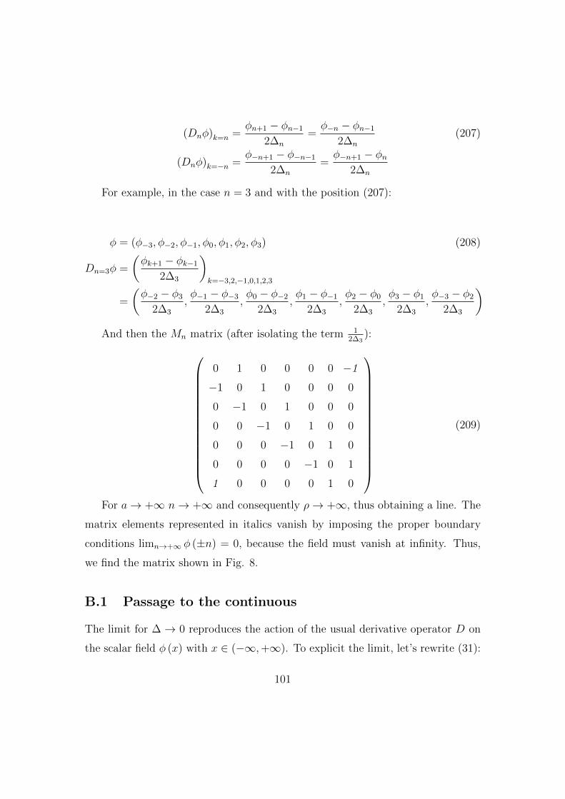
(Dnφ)k=n =φn+1 − φn−1

2∆n

=φ−n − φn−1

2∆n

(207)

(Dnφ)k=−n =φ−n+1 − φ−n−1

2∆n

=φ−n+1 − φn

2∆n

For example, in the case n = 3 and with the position (207):

φ = (φ−3, φ−2, φ−1, φ0, φ1, φ2, φ3) (208)

Dn=3φ =

(φk+1 − φk−1

2∆3

)k=−3,2,−1,0,1,2,3

=

(φ−2 − φ3

2∆3

,φ−1 − φ−3

2∆3

,φ0 − φ−2

2∆3

,φ1 − φ−1

2∆3

,φ2 − φ0

2∆3

,φ3 − φ1

2∆3

,φ−3 − φ2

2∆3

)And then the Mn matrix (after isolating the term 1

2∆3):

0 1 0 0 0 0 −1

−1 0 1 0 0 0 0

0 −1 0 1 0 0 0

0 0 −1 0 1 0 0

0 0 0 −1 0 1 0

0 0 0 0 −1 0 1

1 0 0 0 0 1 0

(209)

For a→ +∞ n→ +∞ and consequently ρ→ +∞, thus obtaining a line. The

matrix elements represented in italics vanish by imposing the proper boundary

conditions limn→+∞ φ (±n) = 0, because the field must vanish at infinity. Thus,

we find the matrix shown in Fig. 8.

B.1 Passage to the continuous

The limit for ∆ → 0 reproduces the action of the usual derivative operator D on

the scalar field φ (x) with x ∈ (−∞,+∞). To explicit the limit, let’s rewrite (31):

101

(D∞φ)k =1

2∆

+∞∑j=−∞

(δk,j−1 − δk,j+1)φ (xj) (210)

We have:

(Dφ) (x) =1

2lim∆→0

1

∆

+∞∑j=−∞

(δk,j−1 − δk,j+1)φ (xj) (211)

=1

2

+∞∫−∞

a (x, x′)φ (x′) dx′,

since the discrete variable k is now replaced by the continuous variable x. In (211)

the function a (x, x′) is

a (x, x′) = lim∆→0

δ (x− (x′ −∆))− δ (x− (x′ + ∆))

∆(212)

So that:

(Dφ) (x) =1

2lim∆→0

1

∆

+∞∫−∞

δ (x− (x′ −∆))φ (x′) dx′

︸ ︷︷ ︸=I1(x)

−+∞∫−∞

δ (x− (x′ + ∆))φ (x′) dx′

︸ ︷︷ ︸=I2(x)

The integrals are easily computed:

I1 (x) =

+∞∫−∞

δ (x− x′ + ∆)φ (x′) dx′

=

+∞∫−∞

δ (x′ − (x+ ∆))φ (x′) dx′

= φ (x+ ∆) ,

102

in the last step we used the Dirac Delta Function parity: δ (x) ≡ δ (−x). Similarly

the second integral is computed:

I2 (x) = φ (x−∆)

Finally:

(Dφ) (x) = lim∆→0

φ (x+ ∆)− φ (x−∆)

2∆,

that is the definition of the derivative of the function φ (x). The (211) can be

written in matrix form:

Dφ.=

1

2Mϕ∞, (213)

In that equation M is a “continuous” matrix with elements a (x, x′), where x, x′ ∈(−∞,+∞); ϕ∞ is a column array with infinity components continuously variable

from −∞ a +∞ so it will be the column array at the first member.

C Topological Spaces

Let S be a non-empty set and P (S) the set of parts of S (eq. 37).

Definition 22 The set S is a topological space if Θ ⊆ P (S) exists that verifies

the following axioms:

T1 ∅, S ∈ Θ

T2 Xaa∈A ⊂ Θ =⇒⋃a∈A

Xa ∈ Θ, where A ⊆R

T3 Xii∈I ⊂ Θ =⇒⋂i∈I

Xi ∈ Θ, where I ⊂ N

The elements of Θ are named open sets. From the axiom 2 follows that the of a

number (even infinite) of open sets is a an open, while axiom 3 we have that the

103

intersection of a finite number of open sets is open. (S,Θ) is the topological space.

S is called space. The elements of an open set are called points.

For example, for every non-empty set S, we can assume Θ = ∅, S. It is immedi-

ate to verify that Θ obeys the three axioms seen above. The topology determined

by Θ is called trivial topology.

***

In RN the natural topology is euclidean topology. Let’s start from the special case

N = 1.

Observation 23 To prevent confusion with the symbol (a, b) denoting the ordered

pair of elements a e b, we denote by ]a, b[ the open bounded set with extremes

a, b ∈ R.

In R the euclidean topology is:

Θe =

A ⊆ R | A =

⋃i

]ai, bi[

(214)

In other words, Θe is the union of all the open sets of R . More precisely, the (214)

should be redefined:

Θe = A ⊆ R | ∀x ∈ A, ∃ ]a, b[ ⊆ A | x ∈ ]a, b[ (215)

It is easy to verify that (215) satisfies the topological space axioms. Then (R,Θe) is

the euclidean topology on R. In R2 = (x1, x2) | xi ∈ R we assume as a collection

of open sets, the set:

Θe =A ⊆ R2 | ∀P

(xi(0)

)∈ A, ∃S2 (P, δ) ⊆ A

, (216)

being S2 (P, δ) the disk:

S2 (P, δ) =

(x1, x2

)∈ R2 |

2∑i=1

[xi − xi(0)

]2< δ2

(217)

104

From this follows that (R2,Θe) is the euclidean topology on R2. In R3 =

(x1, x2, x3) | xi ∈ R we assume, as a collection of open sets, the set:

Θe =A ⊆ R3 | ∀P

(xi(0)

)∈ A, ∃S3 (P, δ) ⊆ A

, (218)

being:

S3 (P, δ) =

(x1, x2, x3

)∈ R2 |

3∑i=1

[xi − xi(0)

]2< δ2

(219)

From this follows that (R3,Θe) is the euclidean topology on R3.

***

Definition 24 Let (S,Θ) be a topological space. A C subset of S is closed, if S

\ C is open. That is:

C ⊆ S is closed)⇐⇒ (S\C) ∈ Θ (220)

Let’s denote by Θ the collection of closed sets of S :

Θ = C ⊆ S | C is closed (221)

It is S ∈ Θ. In fact, S⊆S is closed if S\S is open. But S\S=∅, for which S ∈ Θ,

as ∅ is both open and closed. This makes the first topological space axiom verified.

More precisely, Θ verifies the following properties:

1. ∅, S ∈ Θ

2. Xaa∈A ⊂ Θ =⇒⋃a∈A

Xa ∈ Θ, dove A ⊆R

i.e. the union of a number (even infinite) of closed sets is a closed set.

3. Xii∈I ⊂ Θ =⇒⋂i∈I

Xi ∈ Θ, dove I ⊂ N

We omit the proof of properties 2 and 3.

105

Observation 25 The collection Θ of the open subsets of S determines an unique

collection Θ of open sets of S . This implies that we can introduce a topology into

S through the collection of closed sets Θ.

In the case of the trivial topology Θ = ∅, S, the collection of closed sets is

Θ = S,∅.

***

Assigned the topological space (S,Θ) , let’s define:

Definition 26 x ∈ S is an interior of X ⊆ S)def⇐⇒ (∃A ∈ Θ | X ⊇ A x

Definition 27 U ⊆ S is a neighbourhood of x ∈ S)def⇐⇒ (x is an interior of U

Then U ⊆ S is a neighbourhood of x ∈ S is ∃A ∈ Θ | U ⊇ A x. In other words,

a neighbourhood of x ∈ S, is every subset S containing an open set that contains

x. The definition (27) generalizes as

Definition 28 U ⊆ S is a neighbourhood of X ⊆ S)def⇐⇒ (∃A ∈ Θ | U ⊇ A ⊇ X

Assigned x ∈ S, let’s say:

Uxdef= U ⊆ S | U is a neighbourhood of x (222)

i.e. let’s call Ux the set whose elements are the neighbourhoods of x.

Proposition 29

B ⊂ S | B ⊃ U ∈ Ux =⇒ B ∈ Ux (223)

C,D ⊂ S | C,D ∈ Ux =⇒ C ∩D ∈ Ux (224)

V ∈ Ux =⇒ ∃W neighbourhood of x | V is a neighbourhood of y, ∀y ∈ W (225)

106

Proof. The (223) proves trivially.

The (224):

C,D ∈ Ux =⇒ ∃A,B ∈ Θ | C ⊇ A x, D ⊇ B x

=⇒ x ∈ A ∩B ⊆ C ∩D =⇒A∩B∈Θ

C ∩D ∈ Ux

The (225):

V ∈ Ux =⇒ ∃A ∈ Θ | x ∈ A ⊆ V =⇒ V is neighbourhood of x, ∀x ∈ A

These propositions follow, which we omit the proof of:

Proposition 30 U ⊆ S is neighbourhood of X ⊆ S)⇐⇒ (U is neighbourhood of x, ∀x ∈ X

Proposition 31 A ⊆ S is open )⇐⇒ (A is neighbourhood of x, ∀x ∈ A

Observation 32 In the case of the trivial topology Θ = ∅, S, it is: Ux = S.For example, if S = N, structuring it along with the trivial topology, it follows that

for an arbitrary n ∈ N, the neighbourhood of n is the same set N.

***

Let (S,Θ) be a topological space.

Definition 33 B ⊆Θ is basis of S if every open set of S is expressed as a union

of elements of B. In symbols:

B ⊆Θ is a basis

of S

def⇐⇒

(∀A ∈ Θ, ∃Ba ∈ B | A =

⋃a

Ba

Definition 34 S has a countable basis)def⇐⇒ (∃B basis of S | card (B) ≤ card (N)

Let’s consider, for example, the discrete topology:

Θd = P (S) (226)

Every subset of S is an open set of S. Specifically, ∀x ∈ S, x is an open set of

S. Every subset x consisting of a single element, is called singlet. A basis of Θd

is B =xx∈S

, i.e. the set of all singlets.

107

D Measurement of a quantum observable: de-

generate eigenvalues

We recall that in case of degeneration, the eigenvalue equations for a self-adjoint

operator A which represents a quantum observable A, are written:

A |ak, r〉 = ak |ak, r〉 , ak ∈ σd(A)

, r = 1, ..., gak

A |a, r〉 = a |a, r〉 , a ∈ σc(A)

, r = 1, ..., ga

where gak and ga are the degrees of degeneration of the eigenvalues ak and a,

respectively. More precisely:

gak = dim (Eak) , ga = dim (Ea)

where Eak , Ea are the eigenspaces associated with the eigenvalues ak and a. For

assigned values of ak, a, the systems of eigenvectors:

|ak, 1〉 , ..., |ak, gak〉 (227)

|a, 1〉 , ..., |ak, ga〉

are linearly independent. In other words, the same eigenvalue ak matches gak

independent eigenstates. In case of degeneration, the development(186) is written:

ψ (x) =N∑k=1

gak∑k=1

ck,ruk,r (x) +

ga∑k=1

∫σc(A)

c (a)ua,r (x) da (228)

being:

uk,r (x) = 〈x|ak, r〉

ua,r (x) = 〈x|a, r〉

108

This implies a further complication compared to the non-degenerated case, when

performing a measurement operation. In fact, in the hypothesis of a purely discrete

spectrum, if the system is in the state

|ψ〉 =N∑k=1

gak∑k=1

ck,r |ak, r〉 (229)

as a consequence of the measurement operation, will be found in one of the eigen-

states |ak, r〉:

|ψ〉 −→mis A

|ak, r〉 , con r ∈ 1, 2, ..., gak (230)

D.1 Reduction of the state vector

The process of reduction of the wave vector or collapse of a function wave, occurs in

the operation of measuring an observable A when the quantum system is in a state

of superposition of eigenstates of A. To fix ideas, suppose that the corresponding

self-adjoint operator A is endowed with a purely discrete spectrum with only 2

only eigenvalues: σ(A)

= a1, a2. So the time-developed state vector at time t

is:

|ψ (t)〉 = c1 (t) |a1〉+ c2 (t) |a2〉 (231)

Then suppose that a measurement made at t∗ gives the result a1, whereas:

|ψ〉 −→mis A

|a1〉 (232)

The coefficients of the linear combination (231) are such that c1 (t∗) = 1, c2 (t∗) =

0. And for every t 6= t∗ they take complex values. Further on:

∀δ > 0, t ∈ (t∗ − δ, t∗) =⇒ |c2 (t∗)| 6= 0

i.e. the function |c2 (t)| has a discontinuity of the first kind at t∗.

109

Figure 18: Time evolution of the module of the complex coefficient c2 (t). At

the instant we measure the observable, |c2 (t)| undergoes a discontinuous leap,

corresponding to the quantum leap ( ref eq: quantum leap). The symbol U denotes

the time evolution generated by the unitary transformation U (t, t0) = e−i H(t−t0),

while R expresses the reduction of the state vector.

In the general case of N ≤ +∞ distinct eigenvalues, and after a measurement

process:

|ψ〉 −→mis A

|an〉 , (233)

the reduction of the vector state expresses the finite discontinuity (at the measure-

ment instant) of the N − n coefficients ck (t), with k ∈ 1, 2, ..., N \ n.

E Measurement of a quantum observable (exam-

ple)

Let’s fix our attention on the MC (∞,∞) matrices (Appendix B.1), whose elements

are factorized as follows:

Mik = MiM∗k −→

continuousM (x, x′) = M (x)M∗ (x′) (234)

110

with the additional request M (x) ∈ L2 (R), in order to impose the normalization

condition:

∫ +∞

−∞|M (x)|2 dx = 1. In general, we can find a quantum system (1-

dimensional) Sq with Hilbert Space H = L2 (R) such that for any observable A,

M (x) comes out to be an eigenstate of A. For example, this system can be a

1-dimensional harmonic oscillator. Let’s suppose that at a given time the wave

function is:

ψ (ξ) =1√2

[u0 (ξ) + u1 (ξ)] , (235)

where u0 (ξ) = 〈ξ|0〉 e u1 (ξ) = 〈ξ|1〉 are the energy eigenfunctions of the ground

state and the state n = 1, respectively. As is well known:

u0 (ξ) =(mωπ

)1/4

e−ξ2/2 ; E0 =

ω2

(236)

u1 (ξ) =1√2

(mωπ

)1/4

ξe−ξ2/2 ; E1 =

3ω2

Hereby ξ is a dimensionless variable (ξ =√

mω x). Let’s suppose that in a

measurement operation of the observable energy the state vector collapses to the

eigenstate |1〉:

|ψ〉 −→mis E

|1〉 (237)

The matrix (234) related to this measure is:

M (ξ, ξ′) =1

2

(mωπ

) 12ξξ′e−

12(ξ2+ξ′2) (238)

The field (238) acting on the wave function ψ (ξ) (235), determines the collapse

through the relation:

Mψ =

+∞∫−∞

M (ξ, ξ′)ψ (ξ′) dξ′ =1√2u1 (ξ) (239)

111

From this it follows that the field M (ξ, ξ′) can be identified with the observer’s

consciousness. Nelle fig. 19-20 is reported the field M (ξ, ξ′) and the eigenfunction

which collapses the wave function following the measurement operation.

Figure 19: Trend of the field (238) in unit = m = ω = 1.

References

[1] Galilei, G.: Dialogo sopra i due massimi sistemi del mondo, Giornata sec-

onda. Landini, Fiorenza/Firenze (1632), Guerneri (1995), 238-241. Crew, H.,

de Salvio, A. (English translation): Dialogue concerning the two chief world

systems, Second day. Dover Publications, New York (1954).

[2] Einstein, A.: Zur Elektrodynamik bewegter Korper. Annalen der Physik,17,

891-921 (1905).

[3] Michelson, A. A., Morley, E. W.: On the Relative Motion of the Earth and the

Luminiferous Aether. American Journal of Science, Third Series, 203, 333-345

(1887).

112

Figure 20: Energy eigenstate with eigenvalue E1 in unit = m = ω = 1

[4] Galilei, G.: Discorsi e dimostrazioni matematiche intorno a due nuove

scienze, 191-196. Elzevir/Elsevier, Leida/Leiden (1638). Crew, H., de Salvio,

A. (English translation): Two New Sciences. Macmillan, New York (1914).

[5] Minkowski, H.: Die Grundgleichungen fr die elektromagnetischen Vorgnge

in bewegten Krpern. Nachrichten von der Gesellschaft der Wissenschaften zu

Gttingen, Mathematisch-Physikalische Klasse, 53111 (1908).

[6] Einstein, A.: Die Grundlage der allgemeinen Relativitatstheorie. Annalen der

Physik, 49, 769-822 (1916).

[7] Planck, M.: Entropy and Temperature of Radiant Heat. Annalen der Physik,

4, 71937 (1900).

[8] Einstein, A.: ber einen die Erzeugung und Verwandlung des Lichtes betref-

fenden heuristischen Gesichtspunkt. Annalen der Physik, 17, 132148 (1905).

[9] Rutherford, E.: The Scattering of Alpha and Beta Particles by Matter and

the Structure of the Atom. Philosophical Magazine, 21 (1911).

[10] Bohr, N.: On the Constitution of Atoms and Molecules. Philosophical Maga-

zine, 26, 1-24, 476-502 (1913).

113

[11] Heisenberg, W.: Physics and Philosophy, Section 3. Harper, New York (1958).

[12] Born, M.: Zur Quantenmechanik der Stovorgnge. Zeitschrift fr Physik, 37,

863867 (1926).

[13] Schrodinger, E.: An Undulatory Theory of the Mechanics of Atoms and

Molecules. Physical Review, 28, 10491070 (1926).

[14] Heisenberg, W.: Uber den anschaulichen Inhalt der quantentheoretischen

Kinematik und Mechanik. Zeitschrift fr Physik, 43, 172198 (1927).

[15] Jordan, P.: Anschauliche Quantentheorie. Springer, Berlin (1936).

[16] Bohr, N.: Light and Life. Nature, 131, 421-423, 457-459 (1933).

[17] Wheeler, A.: The anthropic universe, radio interview. Science show, ABC

Radio National, Australia, February 18, 2006.

[18] Stapp, H.P.: Mind, Matter and Quantum Mechanics. Foundations of Physics,

12, 363-399 (1982).

[19] von Neumann, J.: Mathematical Foundations of Quantum Mechanics. Prince-

ton University Press, Princeton (1932).

[20] Stapp, H.P.: Quantum Theory and the Role of Mind in Nature. Foundations

of Physics, 31, 1465-1499 (2001).

[21] Hagelin, J.: Is consciousness the unified field? A field theo-

rist’s perspective. Maharishi International University, Fairfield, Iowa

(1987), now Maharishi University of Management. Available at URL

http://www.mum.edu/pdf msvs/v01/hagelin.pdf as last accessed on March

29, 2012.

[22] Einstein, A., Podolski, B., Rosen, N.: Can quantum-mechanical description

of physical reality be considered complete? Phys. Rev., 47, 777-780 (1935).

114

[23] Einstein, A., Rosen, N.: The Particle Problem in the General Theory of Rel-

ativity. Phys. Rev., 48, 73-77 (1935).

[24] Bohm, D.: Quantum Theory. Prentice Hall, New York (1951).

[25] Kumar, D.: Quantum. Icon Books, London, 313 (2009).

[26] Aspect, A., Grangier, P., Roger, G.: Experimental realization of Einstein-

Podolsky-Rosen-Bohm Gedankenexperiment: a new violation of Bell’s inequal-

ities. Phys. Rev. Lett. 49, 2, 91-94 (1982).

[27] Bell, J.S.: On the Einstein-Podolsky-Rosen paradox. Physics, 1, 195-200

(1964).

[28] Penrose, R.: Angular Momentum: an approach to combinatorial space-

time. Originally appeared in Quantum Theory and Beyond, edited by Ted

Bastin, Cambridge University Press, 151-180 (1971). Available at URL

http://tinyurl.com/penrose-momento-angolare as last accessed on March 29,

2012.

[29] LaFave, N.J.: A Step Toward Pregeometry I.: Ponzano-Regge Spin Net-

works and the Origin of Spacetime Structure in Four Dimensions. ArXiv:gr-

qc/9310036 (1993). Available at URL http://arxiv.org/abs/gr-qc/9310036 as

last accessed on March 29, 2012.

[30] Reisenberger, M., Rovelli, C.: ’Sum over surfaces’ form of loop quan-

tum gravity. Phys. Rev. D, 56, 3490-3508 (1997). Available at URL

http://arxiv.org/abs/gr-qc/9612035 as last accessed on March 29, 2012.

[31] Engle, G., Pereira, R., Rovelli, C., Livine, E.: LQG vertex with finite Im-

mirzi parameter. Nucl. Phys. B, 799, 136-149 (2008). Available at URL

http://arxiv.org/abs/0711.0146 as last accessed on March 29, 2012.

115

[32] Banks, T., Fischler, W., Shenker, S.H., Susskind, L.: M Theory As A Matrix

Model: A Conjecture. Phys. Rev. D, 55, 5112-5128 (1997). Available at URL

http://arxiv.org/abs/hep-th/9610043 as last accessed on March 29, 2012.

[33] Garrett Lisi, A.: An Exceptionally Simple Theory of Everything.

arXiv:0711.0770 (2007). Available at URL http://arxiv.org/abs/0711.0770 as

last accessed on March 29, 2012.

[34] Nastase, H.: Introduction to Supergravity arXiv:1112.3502 (2011). Available

at URL http://arxiv.org/abs/1112.3502 as last accessed on March 29, 2012.

[35] Sakurai, J.J.: Modern Quantum Mechanics. Addison-Wesley, Boston (1985).

[36] Caldirola, P., Cirelli, R., Prosperi, G.M.: Introduzione alla Fisica Teorica.

BUR (Rizzoli), Milano (1982).

[37] Dirac, P.A.M.: The Principles of Quantum Mechanics. Clarendon Press, Ox-

ford (1930).

[38] Maudlin, T.: Quantum Non-locality and Relativity. 2nd ed., Blackwell Pub-

lishers, Malden (2002).

[39] Penrose, R.: On the Nature of Quantum Geometry. Originally appeared in

Wheeler. J.H.: Magic Without Magic, edited by J. Klauder, Freeman, San

Francisco, 333-354 (1972).

116