The application of remote sensing to monitor loss of kelp ...
36
The application of remote sensing to monitor loss of kelp habitat along the Sussex coastline Alexander James August Briggs August 2020 A thesis submitted for the partial fulfilment of the requirements for the degree of Master of Science at Imperial College London Formatted in the journal style of Methods in Ecology and Evolution Submitted for the MSc in Ecology, Evolution and Conservation
Transcript of The application of remote sensing to monitor loss of kelp ...

The application of remote sensing to monitor loss of kelp habitat
along the Sussex coastline
Alexander James August Briggs
August 2020
A thesis submitted for the partial fulfilment of the requirements for the degree of
Master of Science at Imperial College London
Formatted in the journal style of Methods in Ecology and Evolution
Submitted for the MSc in Ecology, Evolution and Conservation
1
Declaration 1
No primary data collection was undertaken for this project. Zoological Society of London (ZSL) 2
provided data quantifying anthropogenic fishing activity, based on data from Global Fishing Watch 3
(2020). A dataset of processed imagery showing kelp distribution (used for ground truthing) was 4
provided to me by ZSL, based on towed video transects. Additionally, ZSL provided raw video 5
footage for additional transects, which I then analysed. I collated all other data used for this project 6
from multiple sources. Through the biodiversity recording website National Biodiversity Network 7
Atlas (2020), I collated observations of kelp distribution based on records taken by divers 8
(Seasearch, 2019). I collated Sentinel satellite imagery from the Copernicus Open Access Hub 9
(European Space Agency, 2020a). I collated weather and tidal data from the Chimet weather buoy 10
and the weather forecasting and archival website Tides4Fishing (Chimet Support Group, 2020; 11
Tides4Fishing, 2020). I sourced a Digital Elevation Model showing bathymetry, created by 12
OceanWise, from the spatial data repository Edina Digimaps (OceanWise, 2016). I also sourced 13
sediment data, created by British Geological Survey, from Edina Digimaps (British Geological 14
Survey, 2011). Guidance and advice were provided by my internal and external supervisors, Dr. 15
James Rosindell (Imperial College London) and Dr. Chris Yesson (Zoological Society of London). I 16
carried out all data cleaning and analysis. 17
Acknowledgements 18
This project was significantly altered and limited by the national lockdown which took place during 19
the Coronavirus pandemic. This prevented drone surveys and the collection of high-resolution 20
remote sensing and ground truthing data, limiting the scope of this study. Therefore, for their 21
assistance in overcoming these issues, I thank my supervisors, Dr. Rosindell and Dr. Yesson. I 22
also thank my course-mates for their support and advice. 23
Word count: 5,997 24
25
26
27
28
29
30
31
32

2
Abstract 33
Kelp forests, one of the most biodiverse habitats on earth and holding a high ecosystem service 34
value, are declining globally due to climate change and anthropogenic fishing activities. Despite 35
these threats, kelp distributions are often unmonitored, preventing critical conservation action. In the 36
UK, along the Sussex coastline, once abundant kelp forests have declined to functional absence. 37
This thesis established a standardised remote sensing-based monitoring method for this study area, 38
using satellite imagery. Three image classification methods commonly used to study kelp were 39
evaluated. The most accurate, a supervised classification, was then applied to produce a species 40
distribution model, predicting the distribution of over 100km2 of kelp across Sussex. Kelp distribution 41
was positively associated with fishing activity, suggesting that trawling may be linked with kelp 42
decline in this area. However, low model accuracy suggests that these results should be treated with 43
caution. This thesis highlights the limitations of widely available remote sensing data for monitoring 44
sublittoral kelp in turbid waters. The collection of high-quality remote sensing data must be prioritised 45
to monitor the distribution of declining kelp forests and inform conservation efforts. 46
1 Introduction 47
Habitat loss is a critical factor contributing to the current biodiversity crisis (Fahrig, 1997; Pardini, 48
Nichols and Püttker, 2017). To protect biodiversity and ecosystem functioning, conservation must 49
prevent habitat loss (Fahrig, 1997; Brooks et al., 2002). The imperative to identify and halt the decline 50
of threatened habitats is highlighted by the aims of the Red List of Ecosystems (International Union 51
for Conservation of Nature, 2020), and the Convention on Biological Diversity (2018). Kelp forests, 52
declining across their global distribution, exemplify habitat loss which threatens high levels of 53
dependant biodiversity (Dayton et al., 1992; Steneck et al., 2002; Casal, Sánchez-Carnero, et al., 54
2011). 55
Laminariales, known as kelp, are a diverse order of large brown macroalgae (Bolton, 2010). Various 56
species of kelp form forest communities which dominate rocky, sublittoral zones on temperate 57
coastlines (Dayton, 1985; Bolton, 2010). Having a high secondary productivity, kelp forests are some 58
of the most biodiverse habitats on earth. Kelp communities provide nutrition for grazers and increase 59
habitat complexity, supporting species of high ecological and commercial value such as the Atlantic 60
cod (Gadus morhua; Steneck et al., 2002; Smale et al., 2013; Teagle et al., 2017). Christie, 61
Norderhaug and Fredriksen (2009) found, within kelp forests, faunal densities of over 100,000 62
individuals per m2. Other regulating ecosystem services provided by kelp forests include carbon 63
sequestration, wave attenuation, and water filtering (Steneck et al., 2002). Kelp also provide 64
provisioning ecosystem services as a fertiliser, fuel, and food source (Chung et al., 2011; Mac 65
Monagail et al., 2017; FAO, 2018). Due to such high ecological and anthropogenic value, further 66
research to ensure the sustainability of kelp communities is necessary (Mac Monagail et al., 2017). 67
3
Kelp forests around the world are declining due to numerous threats including climate change and 68
anthropogenic activities (Dayton et al., 1992; Steneck et al., 2002; Casal, Sánchez-Carnero, et al., 69
2011). Due to the narrow thermal tolerance of many algal species, sea temperature plays a major 70
role in determining species’ range (Breeman, 1988). Brodie et al., (2014) suggests that due to climate 71
change, southern Atlantic distributions of kelp will disappear. In addition, climate change will 72
decrease carbon sequestration as kelp productivity is reduced at higher temperatures (Chung et al., 73
2011; Pessarrodona et al., 2018). Human activities, such as kelp harvesting, overfishing, and 74
trawling, can also lead to the decline of kelp forests (Steneck et al., 2002). Overfishing, in particular, 75
facilitates the overgrazing of kelp by overabundant sea urchin (class Echinoidea) populations by 76
reducing the prevalence of predatory species such as Atlantic cod (Steneck et al., 2002; Wilmers et 77
al., 2012). Despite the threats these factors pose to global kelp forests, there are few programmes 78
monitoring kelp distribution (Smale et al., 2013; Mora-Soto et al., 2020). This critically impedes 79
conservation efforts (Smale et al., 2013). 80
Standardised monitoring is required to recognise the decline of kelp communities, particularly within 81
UK sub-littoral zones which contain 50% of North Atlantic seaweed species (Yesson et al., 2015a; 82
Teagle et al., 2017). There are 19,000km2 of potential kelp habitat around British and Irish coastlines 83
(Yesson et al., 2015b). However, due to the inaccessibility of marine ecosystems, UK kelp 84
distributions are largely unmonitored (Smale et al., 2013; Yesson et al., 2015b). It is especially 85
important that standardised sublittoral monitoring is carried out in southern England, where UK kelp 86
abundance has rapidly declined (Yesson et al., 2015a). 87
Of the 13 species of kelp found in European waters, three are present along the Sussex coastline, 88
in southern England; tangleweed (Laminaria hyperborea), oarweed (Laminaria digitata) and sugar 89
kelp (Saccharina latissima; Sussex Inshore Fisheries and Conservation Authority, 2020). Until the 90
late 1980s, kelp forests were an abundant habitat in this area, covering approximately 177km2 91
(Davies and Nelson, 2019). In the 1970s, an increase in trawling led to a reduction in kelp forest 92
extent and productivity (Davies and Nelson, 2019). The combination of increasing pressure from 93
fishing practices, the 1987 Great Storm, and reductions in water quality has led to a decline of kelp 94
extent by approximately 95% (Sussex Inshore Fisheries and Conservation Authority, 2020). The 95
most recent estimations of remnant kelp patches totalled 6.28km2 in 2010 (Williams and Davies, 96
2019). Fishing pressure remains a significant threat to remnant kelp, with six coastal communities 97
having active fishing fleets, including 53 trawling vessels (Williams and Davies, 2019). Therefore, 98
these pressures have resulted in the significant alteration of sublittoral habitats in southern England 99
and the loss of ecosystem functioning (Hiscock et al., 2004). 100
Restoration of kelp to historic distributions could provide significant benefits (Sussex Inshore 101
Fisheries and Conservation Authority, 2020). Williams and Davies (2019) valued the current 102
ecosystem services of kelp within Sussex as £79,170 per annum. This took into account its yield, 103
4
support of commercial fisheries, coastal defence, carbon sequestration and maintenance of water 104
quality (Williams and Davies, 2019). This is significantly lower than the annual ecosystem services 105
value for 1987 kelp forest distributions, valued at £3,630,605. If restored to its current hypothetical 106
maximum, ecosystem services could rise to £3,243,886 (Williams and Davies, 2019). Sussex 107
Inshore Fisheries and Conservation Authority (IFCA) have proposed a bylaw banning trawling within 108
4km of the Sussex coastline, which was locally approved in 2020 and currently awaits ministerial 109
approval. (Williams and Davies, 2019). This would protect 308km2 of habitat to facilitate the natural 110
recovery of kelp forests (Williams and Davies, 2019). To monitor kelp abundance and assess the 111
effectiveness of conservation management, remote sensing is often used (Deysher, 1993; Bennion 112
et al., 2019). However, current methodologies and community assessments are based on ad hoc 113
studies, and there is an urgent need for the establishment of a standardised, sublittoral monitoring 114
method for kelp communities (Yesson et al., 2015a; Bennion et al., 2019). 115
Remote sensing is a rapidly emerging tool for conservation research (Turner et al., 2003; Pettorelli, 116
Safi and Turner, 2014). Since the 1970s, studies on kelp using remote sensing have predominantly 117
used satellites to monitor inaccessible sublittoral communities over large spatial scales (Jensen, 118
Estes and Tinney, 1980; Deysher, 1993; Bennion et al., 2019). Resulting imagery can be used to 119
detect macroalgae and produce species distribution models (SDMs) to aid conservation (Jensen, 120
Estes and Tinney, 1980; Belsher and Mouchot, 1992; Deysher, 1993; Guillaumont, Callens and 121
Dion, 1993). However, due to varying requirements in monitoring kelp under different sublittoral 122
conditions, there is no standardised methodology (Kellaris et al., 2019; Mora-Soto et al., 2020). 123
1.1 Aims and Objectives 124
In this thesis, I aim to develop a remote sensing-based monitoring method and produce a distribution 125
estimate for kelp along the Sussex coastline. I then aim to apply this to investigate the extent to 126
which current kelp distributions are impacted by anthropogenic fishing activities. This will be 127
undertaken via several methods of classifying satellite imagery, testing resultant kelp distribution 128
models against ground truthing data, and comparing the area of kelp patches with the spatial 129
distribution of fishing activities. I investigate the hypotheses that: i) satellite imagery can be used to 130
provide a reliable estimate of kelp distribution, and that ii) fishing activities continue to impact kelp 131
along the Sussex coastline. 132
133
134
135
136

5
2 Methodology 137
2.1 Study area 138
I conducted this study on approximately 200km of Sussex coastline, covering an area of 10,463km2. 139
I collected data layers within a study area polygon created in QGIS 3.0.2 (QGIS Development Team, 140
2020), and cropped layers to a polygon of land above the mean (springs) high water height (Holmes, 141
2017) using the package ‘raster’ v3.3-13 (Hijmans, 2020). To give an accurate representation of 142
spatial scale, I reprojected data from the global projection system WGS84 to the local projection 143
system British National Grid, interpolating new values from the original data, using the package 144
‘rgdal’ v1.5-15 (Bivand, Keitt and Rowlingson, 2020). Analyses were performed in R v3.6.0 (R Core 145
Team, 2019) using RStudio v1.3.1056 (RStudio Team, 2020). 146
Figures were created using the package ‘ggplot2’ v3.3.2 (Wickham, 2016), with north arrows and 147
scale bars added using the packages ‘GISTools’ v0.7-4 (Brunsdon and Chen, 2014) and ‘ggspatial’ 148
v1.1.4 (Dunnington, 2020). Data labels were added using the ‘ggrepel’ v0.8.2 (Slowikowski, 2020) 149
package, and accessible palettes were used through the package ‘RColorBrewer’ v1.1-2 (Neuwirth, 150
2014). 151
2.2 Ground truthing data 152
I collated ground truthing points from towed video collected by Sussex IFCA and Zoological Society 153
of London (ZSL) on 21st April 2013, cleaning and manipulating dataframes using the packages ‘tidyr’ 154
v1.1.0 (Wickham and Henry, 2020), ‘dplyr’ v1.0.1 (Wickham et al., 2020), ‘data.table’ v1.13.0 (Dowle 155
and Srinivasan, 2020), and ‘varhandle’ v2.0.5 (Mahmoudian, 2020). A sledge mounted camera was 156
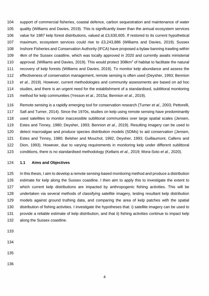
towed along the seabed at a constant speed. This was attached to a research vessel by a cable 157
approximately 10m long. Surveying occurred at 16 stations (transects) off Selsey. The research 158
vessel recorded depth, time and coordinates at the start and end of each transect. Coordinates were 159
corrected to estimate the position of the towed camera (Figure 1). This lag in position (1) was 160
calculated, based on Pythagoras’ theorem, and using known depth (Z) and cable length (C) values, 161
assuming the cable to be virtually straight, as: 162
𝐿𝑎𝑔2 = 𝑍2 + 𝐶2 163
164
(1)
6
165
Still images were extracted from the footage at approximately 20s intervals, selected when the 166
seabed was clearly visible. For each image, the time and species present were noted. For use in 167
figures, percentage cover was noted and translated into abundance using the SACFOR abundance 168
classification scale for sublittoral flora (Hiscock, 1996). The time elapsed per image was multiplied 169
by speed to calculate the distance along the transect, using the package ‘chron’ v2.3-55 (James and 170
Hornik, 2020). This was combined with start coordinates of the boat, camera lag and bearing to 171
provide coordinates for each image using the package ‘geosphere’ v1.5-10 (Hijmans, 2019) to 172
account for the earth’s curvature. I used this method to analyse data from three stations and was 173
provided with pre-analysed data for 13 stations by ZSL. I plotted these coordinates as vector data 174
(spatial coordinates) using the packages ‘sp’ v1.4-2 (Pebesma and Bivand, 2005) and ‘sf’ 0.9-5 175
(Pebesma, 2018), and assigned a binary value, kelp present or absent, depending on whether the 176
image contained kelp. 177
I collated observations of Laminaria spp. based on records taken by divers (Seasearch, 2019), from 178
the biodiversity recording website, National Biodiversity Network Atlas (NBN; 2020). While the spatial 179
accuracy of these observations was too low for analysis (>10m), they were used to illustrate possible 180
kelp distribution. I removed observations taken prior to the year 2000, that were considered unlikely 181
to represent current distributions. 182
2.3 Remote sensing data 183
Imagery, collected by the Sentinel satellite constellation, was collated by myself from the Copernicus 184
Open Access Hub (European Space Agency, 2020a). At a 10x10m resolution, four spectral bands 185
Figure 1: Diagram illustrating towed camera surveys carried out to detect kelp
(Laminaria spp.), with the camera position calculated using known values of cable
length and depth.
7
were available (Red, Green, Blue and Near Infra-Red), with six additional bands (four visible and 186
near-infrared, and two short-wave infrared bands) at 20x20m resolution (European Space Agency, 187
2020a, Supplementary Information 1). I selected Sentinel Level 2a imagery which provided bottom-188
of-atmosphere reflectance values with atmospheric water vapour correction and orthorectification 189
(correcting for perspective) carried out (European Space Agency, 2015). I extracted, and combined 190
by date, image tiles unobscured by dense cloud (<30% coverage). I calculated mean windspeed and 191
wave height, factors which increase turbidity and suspended sediment in the water column, using 192
records from the Chimet weather buoy, situated at the mouth of Chichester Harbour (Chimet Support 193
Group, 2020). These values were calculated for two days prior to image collection. I took tide height 194
at the time of data collection for Selsey from Tides4Fishing (Tides4Fishing, 2020). Reflectance 195
values extracted from satellite images with high turbidity or suspended sediment in the water column 196
were likely to be non-representative of the seabed. I selected multiple images where conditions 197
minimised water depth, turbidity, and suspended sediment, and plotted them as spatial raster data 198
(pixel-based imagery) using the ‘raster’ package. 199
From Edina Digimaps (OceanWise, 2016), I sourced a 30x30m resolution Digital Elevation Model 200
raster showing bathymetry (seabed depth) which was created by OceanWise, based on combined 201
multibeam acoustic and LIDAR data. I altered bathymetry using bilinear interpolation to match the 202
satellite imagery resolution, creating more pixels with the same values, using the package ‘gdalUtils’ 203
v2.0.3.2 (Greenberg and Mattiuzzi, 2020). 204
I sourced vector data identifying seabed sediment classes from Edina Digimaps, created by British 205
Geological Survey based on sediment samples (British Geological Survey, 2011). Raster data of 206
25x25m resolution quantifying fishing activity over 1,706.74km2 of the study area, was provided by 207
ZSL. This data calculated fishing activity as the annual average number of fishing vessels observed, 208
based on vessel GPS tracking data collected by Global Fishing Watch (Global Fishing Watch, 2020). 209
2.4 Image classification 210
I ran three pixel-based classification methods commonly used to study kelp: an index classification 211
(Hu, 2009; Garcia and Sitjar, 2020; Mora-Soto et al., 2020), alongside two machine learning 212
algorithms; a supervised (Casal, Sánchez-Carnero, et al., 2011; Brodie et al., 2018; Kellaris et al., 213
2019) and unsupervised classification (Van der Wal et al., 2014; Yesson, Ash and Brodie, 2015). 214
For index-based classification, I used the Kelp Difference index (KD), designed to identify the 215
spectral signature of kelp (Mora-Soto et al., 2020). KD (2) was calculated as the difference in 216
reflectance values between infra-red (RB6), and red (RB4) satellite image bands: 217
𝐾𝐷 = 𝑅𝐵6 − 𝑅𝐵4 218
Unsupervised classification was conducted using machine learning algorithms which classify image 219
pixels based on a specified number of clusters. K-means clustering partitions data into a specified 220
(2)
8
number of clusters by maximising intra-class similarity and minimising inter-class similarity 221
(MacQueen, 1967). This algorithm randomly selected observations as cluster centroids and 222
assigned observations to clusters by minimising the Euclidean distance between the observation 223
and the centroid. New cluster centroids (means) were then calculated. Clustering Large Applications 224
(CLARA) is a similar method designed to deal with large datasets (>1,000 observations; Kaufman 225
and Rousseeuw, 1990). This algorithm randomly subsampled the data, creating a specified number 226
of clusters. One observation per cluster was randomly selected as a medoid, an observation within 227
the dataset with minimal dissimilarity between all observations within the cluster. The entire dataset 228
was then assigned to medoids. Both algorithms iterated until cluster assignments converged. I 229
repeated K-means and CLARA clustering, specifying 2-8 clusters based on Van der Wal et al. 230
(2014), using the package ‘cluster’ v2.1.0 (Maechler et al., 2019). I selected the clustering algorithm 231
and number of clusters which maximised the highest average similarity of observations to their 232
clusters (silhouette index), using the packages ‘clusterCrit’ v1.2.8 (Desgraupes, 2018) and ‘knitr’ 233
v1.29 (Xie, 2020). I assigned clusters as kelp present/absent, depending on which cluster included 234
the most ground truthing observations of kelp. 235
Supervised classification was conducted using a Support Vector Machine (SVM) learning algorithm 236
which produces a predictive model trained on ground truthing data. To train the model, I extracted 237
the median cell values of each satellite image within a 10m radius (known as a “buffer”) of each 238
ground truthing point containing kelp, using the ‘raster’ package. Cells overlapping the buffer edges 239
were included in the median. I then divided ground truthing points at random, with 25% as a training 240
dataset, and 75% for model validation, based on Brodie et al. (2018). I then ran an SVM to find a 241
hyperplane which best differentiated classes within the training dataset, using the package ‘e1071’ 242
v1.7-3 (Meyer et al., 2019). The hyperplane was determined based on gamma (Ɣ) and cost (C) 243
values. Ɣ determines the influence of individual observations on fitting the hyperplane, which if too 244
large may excessively delineate data and lead to overfitting. C determines the cost of 245
misclassification by specifying the size of the hyperplane margin, within which points may be 246
misclassified. I selected the optimal gamma and cost parameters by testing combinations of a range 247
of values (gamma: 2−13-210 cost: 2−5-210) to produce predictions with the highest percentage 248
agreement with training data. I then ran the SVM using the optimal parameters, which predicted 249
classes across the entire satellite image. 250
I ran all three classification methods on each satellite image. To test the accuracy of models against 251
ground truthing points, I extracted the median cell values of each model within a 10m buffer of each 252
point. A 10m buffer was chosen to match model resolutions. For supervised classification models, I 253
used 75% of the ground truthing data (see above). I then assigned these values a binary predicted 254
category, kelp present or absent. I created a confusion matrix for each model run on each satellite 255
image, comparing expected categories from ground truthing data to categories predicted by the 256
model. These matrices, using the number of observations (N) and categories (k), gave the number 257

9
of times the final model (i) correctly predicted category (nki). I then calculated (3) the probability of 258
agreement (Po), and (4) probability of random agreement (Pe), to produce (5) a Cohen’s Kappa value 259
(Cohen, 1960) to test whether satellite imagery can provide a reliable estimate of kelp distribution: 260
𝑃𝑜 =𝑛𝑘𝑖
𝑁 261
𝑃𝑒 =1
𝑁2∑ 𝑛𝑘1𝑛𝑘2
𝑘
262
𝐾𝑎𝑝𝑝𝑎 =𝑃𝑜 − 𝑃𝑒
1 − 𝑃𝑒 263
Kappa values of 1 suggested a perfect agreement between a model and ground truthing data. I then 264
selected the model and satellite image with the highest Kappa value to predict kelp distribution. 265
2.5 Water attenuation correction 266
Light passing through a water column is attenuated (absorbed and scattered) due to suspended 267
material and the refractive properties of water (Kirk, 1994). Therefore, it may be important to correct 268
this effect in data in order to produce accurate classifications (Kirk, 1994). Lyzenga's equation 269
(Lyzenga, 1978, 1981) is the most commonly used method to correct for light attenuation in the water 270
column and increase the accuracy of seabed classification (Zoffoli, Frouin and Kampel, 2014). This 271
was adapted by Sagawa et al. (2010) to study coastal ecosystems, accounting for water with low 272
transparency by including depth: 273
𝑋𝑖 =(𝐿𝑖 − 𝐿𝑠𝑖)
exp (−𝐾𝑖𝑔𝑍) 274
The corrected values of seabed reflectance (Xi) were calculated for each satellite image spectral 275
band (i) using reflectance (Li), deep water radiance (Lsi), the rate of light attenuation in the water 276
column (Ki, attenuation coefficient, m-1), the path length of light passing through the water column 277
(g) and water depth (Z). I extracted depth data (Z) from the bathymetry raster and added tide height 278
at the time the satellite image was collected using the ‘raster’ package. I assumed that Z was 279
equivalent to g and therefore, to produce negative depth values, took g as -1. I calculated attenuation 280
coefficients (Ki) by assuming that variations in reflectance values over bare sand were due to 281
attenuation over varying water depths. I identified bare sand as points in QGIS, where the seabed 282
was classed as sand by sediment vector data and where sand was visually identifiable in satellite 283
imagery. To find the rate of light attenuation, I ran a linear model, taking reflectance value as the 284
response variable, and depth as the explanatory variable, for each spectral band of the satellite 285
imagery. To give an indication of correction accuracy, I compared the expected relative attenuation 286
rates for the spectral bands to the model slopes. I calculated deep-water radiance (Lsi) by taking the 287
mean reflectance values for deep-water areas within the lowest 10th percentile of depth values, 288
(3)
(6)
(4)
(5)
10
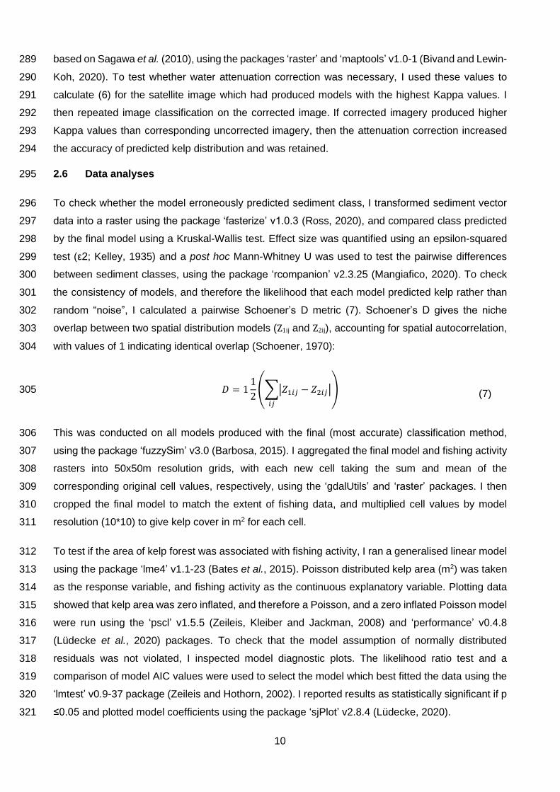
based on Sagawa et al. (2010), using the packages ‘raster’ and ‘maptools’ v1.0-1 (Bivand and Lewin-289
Koh, 2020). To test whether water attenuation correction was necessary, I used these values to 290
calculate (6) for the satellite image which had produced models with the highest Kappa values. I 291
then repeated image classification on the corrected image. If corrected imagery produced higher 292
Kappa values than corresponding uncorrected imagery, then the attenuation correction increased 293
the accuracy of predicted kelp distribution and was retained. 294
2.6 Data analyses 295
To check whether the model erroneously predicted sediment class, I transformed sediment vector 296
data into a raster using the package ‘fasterize’ v1.0.3 (Ross, 2020), and compared class predicted 297
by the final model using a Kruskal-Wallis test. Effect size was quantified using an epsilon-squared 298
test (ε2; Kelley, 1935) and a post hoc Mann-Whitney U was used to test the pairwise differences 299
between sediment classes, using the package ‘rcompanion’ v2.3.25 (Mangiafico, 2020). To check 300
the consistency of models, and therefore the likelihood that each model predicted kelp rather than 301
random “noise”, I calculated a pairwise Schoener’s D metric (7). Schoener’s D gives the niche 302
overlap between two spatial distribution models (Z1ij and Z2ij), accounting for spatial autocorrelation, 303
with values of 1 indicating identical overlap (Schoener, 1970): 304
𝐷 = 11
2(∑|𝑍1𝑖𝑗 − 𝑍2𝑖𝑗|
𝑖𝑗
) 305
This was conducted on all models produced with the final (most accurate) classification method, 306
using the package ‘fuzzySim’ v3.0 (Barbosa, 2015). I aggregated the final model and fishing activity 307
rasters into 50x50m resolution grids, with each new cell taking the sum and mean of the 308
corresponding original cell values, respectively, using the ‘gdalUtils’ and ‘raster’ packages. I then 309
cropped the final model to match the extent of fishing data, and multiplied cell values by model 310
resolution (10*10) to give kelp cover in m2 for each cell. 311
To test if the area of kelp forest was associated with fishing activity, I ran a generalised linear model 312
using the package ‘lme4’ v1.1-23 (Bates et al., 2015). Poisson distributed kelp area (m2) was taken 313
as the response variable, and fishing activity as the continuous explanatory variable. Plotting data 314
showed that kelp area was zero inflated, and therefore a Poisson, and a zero inflated Poisson model 315
were run using the ‘pscl’ v1.5.5 (Zeileis, Kleiber and Jackman, 2008) and ‘performance’ v0.4.8 316
(Lüdecke et al., 2020) packages. To check that the model assumption of normally distributed 317
residuals was not violated, I inspected model diagnostic plots. The likelihood ratio test and a 318
comparison of model AIC values were used to select the model which best fitted the data using the 319
‘lmtest’ v0.9-37 package (Zeileis and Hothorn, 2002). I reported results as statistically significant if p 320
≤0.05 and plotted model coefficients using the package ‘sjPlot’ v2.8.4 (Lüdecke, 2020). 321
(7)

11
3 Results 322
3.1 Ground truthing data 323
Ground truthing from towed camera surveys included kelp presence observations, (n=74) averaging 324
6.17 observations per transect (SD: 5.57, range: 1-17), and kelp absence observations (n=113). 325
Additionally, I collated 154 observations of kelp from NBN (Figure 2). 326
327
3.2 Remote sensing data 328
Of the satellite images collated (N=7), four were collected during suitable conditions and used for 329
classification (Supplementary Information 2). These images were acquired on 20.07.2020, 330
21.04.2020, 26.02.2019, and 22.04.2018. 331
332
333
334
(A)
(B)
Figure 2: Maps of kelp (Laminaria spp.) presence along the Sussex coast, coloured by
abundance. Data were based on (A) towed camera surveys carried out by Zoological
Society of London and (B) citizen science data from divers collated from National
Biodiversity Network (2020). The blue line indicates the area where trawling will be
banned to protect kelp.
Hastings
Selsey
Chichester Brighton
Hastings
Selsey
Chichester Brighton
12
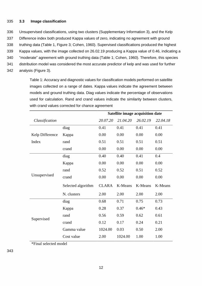
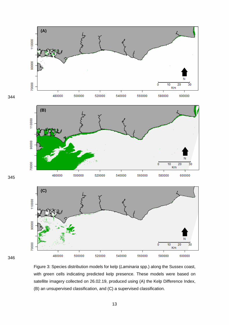
3.3 Image classification 335
Unsupervised classifications, using two clusters (Supplementary Information 3), and the Kelp 336
Difference index both produced Kappa values of zero, indicating no agreement with ground 337
truthing data (Table 1, Figure 3; Cohen, 1960). Supervised classifications produced the highest 338
Kappa values, with the image collected on 26.02.19 producing a Kappa value of 0.46, indicating a 339
“moderate” agreement with ground truthing data (Table 1; Cohen, 1960). Therefore, this species 340
distribution model was considered the most accurate predictor of kelp and was used for further 341
analysis (Figure 3). 342
Satellite image acquisition date
Classification 20.07.20 21.04.20 26.02.19 22.04.18
Kelp Difference
Index
diag 0.41 0.41 0.41 0.41
Kappa 0.00 0.00 0.00 0.00
rand 0.51 0.51 0.51 0.51
crand 0.00 0.00 0.00 0.00
Unsupervised
diag 0.40 0.40 0.41 0.4
Kappa 0.00 0.00 0.00 0.00
rand 0.52 0.52 0.51 0.52
crand 0.00 0.00 0.00 0.00
Selected algorithm CLARA K-Means K-Means K-Means
N. clusters 2.00 2.00 2.00 2.00
Supervised
diag 0.68 0.71 0.75 0.73
Kappa 0.28 0.37 0.46* 0.43
rand 0.56 0.59 0.62 0.61
crand 0.12 0.17 0.24 0.21
Gamma value 1024.00 0.03 0.50 2.00
Cost value 2.00 1024.00 1.00 1.00
*Final selected model
343
Table 1: Accuracy and diagnostic values for classification models performed on satellite
images collected on a range of dates. Kappa values indicate the agreement between
models and ground truthing data. Diag values indicate the percentage of observations
used for calculation. Rand and crand values indicate the similarity between clusters,
with crand values corrected for chance agreement
13
344
345
346
(A)
(B)
(C)
Figure 3: Species distribution models for kelp (Laminaria spp.) along the Sussex coast,
with green cells indicating predicted kelp presence. These models were based on
satellite imagery collected on 26.02.19, produced using (A) the Kelp Difference Index,
(B) an unsupervised classification, and (C) a supervised classification.
14
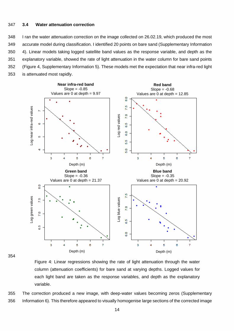
3.4 Water attenuation correction 347
I ran the water attenuation correction on the image collected on 26.02.19, which produced the most 348
accurate model during classification. I identified 20 points on bare sand (Supplementary Information 349
4). Linear models taking logged satellite band values as the response variable, and depth as the 350
explanatory variable, showed the rate of light attenuation in the water column for bare sand points 351
(Figure 4, Supplementary Information 5). These models met the expectation that near infra-red light 352
is attenuated most rapidly. 353
354
The correction produced a new image, with deep-water values becoming zeros (Supplementary 355
Information 6). This therefore appeared to visually homogenise large sections of the corrected image 356
Near infra-red band Slope = -0.85
Values are 0 at depth = 9.97
Red band Slope = -0.68
Values are 0 at depth = 12.85
Green band Slope = -0.36
Values are 0 at depth = 21.37
Blue band Slope = -0.35
Values are 0 at depth = 20.92
Lo
g b
lue
va
lues
Lo
g g
ree
n v
alu
es
Lo
g r
ed
va
lues
Lo
g n
ea
r in
fra
-red
va
lue
s
Depth (m) Depth (m)
Depth (m) Depth (m)
Figure 4: Linear regressions showing the rate of light attenuation through the water
column (attenuation coefficients) for bare sand at varying depths. Logged values for
each light band are taken as the response variables, and depth as the explanatory
variable.
15
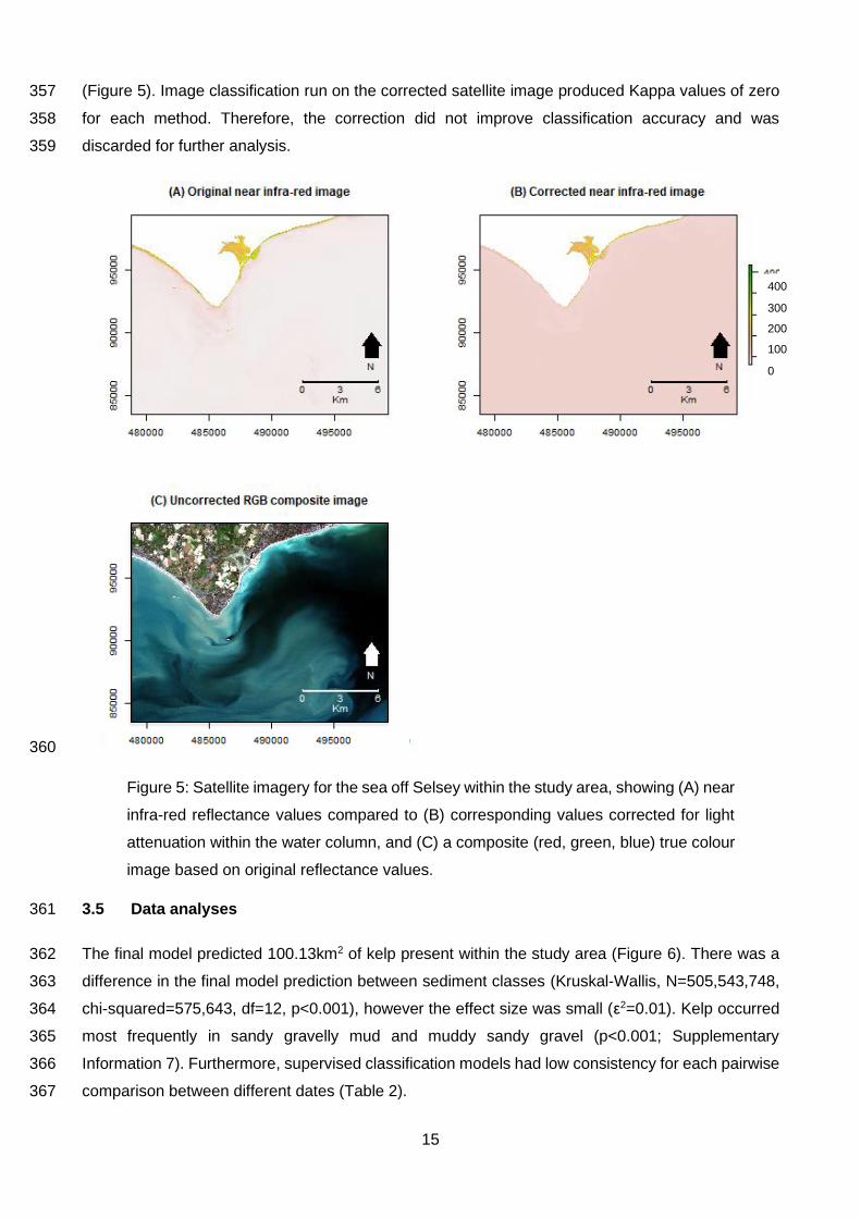
(Figure 5). Image classification run on the corrected satellite image produced Kappa values of zero 357
for each method. Therefore, the correction did not improve classification accuracy and was 358
discarded for further analysis. 359
360
3.5 Data analyses 361
The final model predicted 100.13km2 of kelp present within the study area (Figure 6). There was a 362
difference in the final model prediction between sediment classes (Kruskal-Wallis, N=505,543,748, 363
chi-squared=575,643, df=12, p<0.001), however the effect size was small (ε2=0.01). Kelp occurred 364
most frequently in sandy gravelly mud and muddy sandy gravel (p<0.001; Supplementary 365
Information 7). Furthermore, supervised classification models had low consistency for each pairwise 366
comparison between different dates (Table 2). 367
400
300
200
100
0
400
300
200
100
0
Figure 5: Satellite imagery for the sea off Selsey within the study area, showing (A) near
infra-red reflectance values compared to (B) corresponding values corrected for light
attenuation within the water column, and (C) a composite (red, green, blue) true colour
image based on original reflectance values.
16
368
Satellite imagery
acquisition date
22.04.18 26.02.19 21.04.20 20.07.20
22.04.18 -- 0.01 0.02 0.03
26.02.19 0.01 -- 0.04 0.01
21.04.20 0.02 0.04 -- 0.09
20.07.20 0.03 0.01 0.09 --
369
For the linear model using observations taken per 50*50m area (N=591,654), the average area of 370
kelp was 113.24m2 (SD: 454.95, range: 0.00-2500.00) and average fishing activity was 3.90 (SD: 371
6.50, range: 0.00-72.71, Figure 7). Goodness of fit was assessed, and a zero-inflated Poisson model 372
selected (likelihood ratio test, chi2 = 2.65x10⁸, df = 2, p=<0.001). I found a positive, statistically 373
significant association between predicted kelp area and observed fishing activity (Table 3). An 374
increase in 1 vessel/year resulted in a 92% increase in kelp area. An adjusted R2 of 1.00 indicated 375
the model fit the data well. 376
Table 2: Correlation matrix for supervised classification models for satellite imagery,
produced using the Schoener’s D metric for spatial niche overlap, with values of 1
indicating identical overlap (Schoener, 1970).
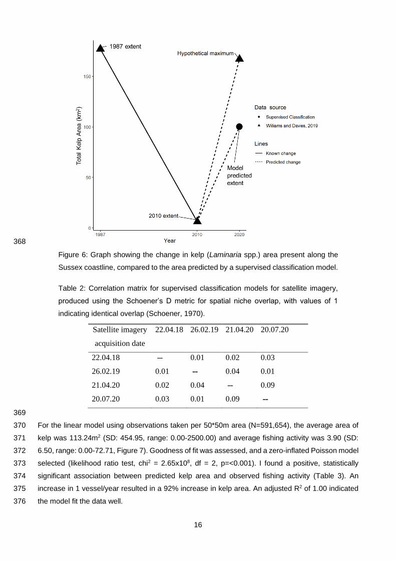
Figure 6: Graph showing the change in kelp (Laminaria spp.) area present along the
Sussex coastline, compared to the area predicted by a supervised classification model.

17
377
Kelp area (m2)
Predictors Incidence Rate Ratios CI p
(Intercept) 4.97 4.92 – 5.03 <0.001
Fishing activity 1.92 1.90 – 1.94 <0.001
Observations 591,654
R2 / R2 adjusted 1.00 / 1.00
378
379
380
381
382
383
384
Table 3: Outputs of a linear regression (zero-inflated Poisson model) showing how area
of kelp (Laminaria spp.) forest is associated with fishing activity (average vessels/year).
Figure 7: Raster data showing fishing activity. This was calculated as the average
annual number of fishing vessels observed per 25x25m cell, based on vessel GPS
tracking (Global Fishing Watch, 2020).
18
4 Discussion 385
In this thesis, I evaluated remote sensing-based methods commonly used to monitor kelp distribution 386
and identify supervised classification as the most appropriate for studying kelp in Sussex. I produced 387
a species distribution model for kelp and found that kelp distribution is related to anthropogenic 388
fishing activity along the Sussex coastline. 389
The final species distribution model predicted kelp with an accuracy comparable to Kappa values 390
reported by other studies (Van der Wal et al., 2014; Brodie et al., 2018; Mora-Soto et al., 2020). 391
However, while Kappa values are the most common statistic used to report classification accuracy, 392
several studies suggest that their categorisation is lenient, allowing inaccurate models to be treated 393
as accurate (Bruckner and Yoder, 2006; McHugh, 2012). Following the suggested categorisation of 394
Kappa values by McHugh (2012), the agreement between ground truthing data and my final SDM 395
would instead be classed as “weak”, suggesting that my model should be treated with caution. My 396
final SDM predicts kelp in areas of historic kelp distribution (Williams and Davies, 2019) and follows 397
a similar distribution to citizen science data (Figure 2). However, my model suggests that kelp forest 398
area has recovered by 1,594% since 2010. While this is lower than the hypothetical maximum 399
distribution of kelp, the recovery predicted by my model is unlikely as there has been little 400
conservation action or alteration to fishing pressure (Williams and Davies, 2019). 401
My results showed that fishing activity was significantly positively associated with kelp presence. 402
This suggests that fishing activity is directed towards areas of remnant kelp forest, and therefore 403
fishing continues to impact kelp along the Sussex coast. Further research is required to determine 404
relationship directionality, which may also be due to fishing activity promoting kelp development. 405
However, this is highly unlikely as studies have shown kelp forests take several years to recover 406
from damage caused by trawling (Christie, Fredriksen and Rinde, 1998; Steen et al., 2016). It is also 407
possible that my model erroneously predicts features other than kelp, such as different algal species 408
or the elevated roughness of trawled seabed (Smith et al., 2003; Brodie et al., 2018). If model 409
variables are both indicators of fishing activity, this would explain the biologically improbable high R2 410
value (Table 3). However, any conclusions drawn from the correlation between fishing and kelp 411
distribution are limited by the low accuracy of my final model. 412
4.1 Limitations 413
The low accuracy of my model may be due to multiple factors such as patches of kelp smaller than 414
imagery pixels, which may result in the misclassification of features other than kelp (Brodie et al., 415
2018). While the model predictions differed between sediment classes, this may be due to the high 416
sample size resulting in a false positive result, and the effect size was small. Similarly, high turbidity 417
may reduce the visibility of the seabed through the water column (Kutser, Vahtmäe and Martin, 418
2006). The attenuation correction found that light was attenuated at shallower depths than many 419

19
kelp patches identified by ground truthing. Near infra-red and red bands are important in detecting 420
kelp and other vegetation (Hu, 2009; Mora-Soto et al., 2020). However, these bands were affected 421
by high rates of light attenuation, suggesting that deep areas had “true” reflectance values of zero. 422
Models may therefore be classifying spectral noise, values not representative of the seabed, 423
supported by the low consistency between models (Sagawa et al., 2010). This would explain the 424
failure of the Kelp Difference Index, unsupervised classification, and water attenuation correction, to 425
produce Kappa values greater than zero. Due to low model accuracy, this study cannot accept the 426
hypotheses that satellite imagery can be used to provide a reliable estimate of kelp distribution and 427
is unable to determine whether fishing activities continue to impact kelp along the Sussex coastline. 428
My model’s accuracy could be improved by multiple methods. More ground truthing data, collected 429
recently and with a wider distribution across the study area, may provide a training dataset more 430
representative of the spectral signature of kelp in Sussex and improve supervised classification 431
(Abburu and Golla, 2015). Similarly, the Kelp Difference Index was designed to identify the spectral 432
signature of giant kelp (Macrocystis pyrifera; Mora-Soto et al., 2020). An index adjusted to identify 433
the spectral signature of kelp species present in Sussex (tangleweed, oarweed and sugar kelp) may 434
increase the accuracy of index-based classification (Hu, 2009). Unsupervised classification is 435
subject to human error during the manual assignment of habitat classes to predicted clusters (Abburu 436
and Golla, 2015), however there was little ambiguity in this study. While each classification may be 437
adapted to improve accuracy, the major limitation to this study was spectral noise within satellite 438
imagery. This study attempted to identify kelp in smaller patches and within deeper water than many 439
concurrent studies (Casal, Sánchez-Carnero, et al., 2011; Mora-Soto et al., 2020). Under such 440
conditions, the lack of accurate seabed reflectance values, along with insufficient resolutions, may 441
have prevented accurate classification (Sagawa et al., 2010; Zoffoli, Frouin and Kampel, 2014). 442
Higher resolution data, collected under suitable conditions to reduce water column turbidity, may 443
ensure the classification of accurate seabed reflectance values and improve model accuracy (Brodie 444
et al., 2018; Bennion et al., 2019). 445
4.2 Implications and future research 446
The species distribution model produced by this study does not have sufficient accuracy to inform 447
Sussex IFCA’s monitoring programme. At most, this model could be used to inform stratified diving 448
or towed camera surveys to confirm the presence of kelp. My results support Bennion et al. (2019), 449
suggesting that traditional, direct observation surveys remain the “gold standard” of monitoring 450
macroalgae due to limited confidence in remote sensing derived predictions. While the lack of 451
standardisation for imagery classification to identify kelp has been criticised by several studies 452
(Bennion et al., 2019; Kellaris et al., 2019; Mora-Soto et al., 2020), the methods used in this study 453
have been previously used to successfully identify kelp distributions in other areas (Yesson, Ash and 454
Brodie, 2015; Brodie et al., 2018; Kellaris et al., 2019; Mora-Soto et al., 2020). I suggest that the 455
20
quality of widely available remote sensing data remains the major limitation of remote sensing to 456
produce SDMs for sublittoral kelp. Satellite images for subtidal remote sensing should be selected 457
to account for many confounding factors, including cloud cover, tide height, and sea state (Kutser, 458
Vahtmäe and Martin, 2006; Casal, Sánchez-Carnero, et al., 2011). However, satellite imagery is not 459
targeted at coastal areas, often resulting in suboptimal images with high turbidity and light 460
attenuation (Yesson, Ash and Brodie, 2015; Bennion et al., 2019). This limitation highlights the need 461
for remote sensing methods with high spatial resolutions, targeted to meet the study-specific 462
requirements of monitoring kelp forests. 463
Remote sensing platforms which offer alternatives to satellites could increase the application of 464
remote sensing. Satellite imagery provides repeated, global coverage with high spectral resolutions 465
(Hu, 2009; Casal, Kutser, et al., 2011; Yesson, Ash and Brodie, 2015; Mora-Soto et al., 2020). 466
However, while continually improving, the spatial resolution of widely available satellite imagery may 467
be insufficient for the detection of small kelp forest patches. While macroalgae SDMs have been 468
produced using satellite imagery with low spatial resolutions (>300m; Kutser, Vahtmäe and Martin, 469
2006; Hu, 2009), it is not possible to detect patches <10 hectares at resolutions <20m (Deysher, 470
1993; Kellaris et al., 2019). Planes and drones offer cost effective methods to map kelp distribution 471
at higher resolutions than widely available satellite imagery (<100cm; Deysher, 1993; Volent, 472
Johnsen and Sigernes, 2007; Brodie et al., 2018; Kellaris et al., 2019). Furthermore, unlike satellite 473
orbits, plane and drone surveys may be timed to coincide with optimal tidal and weather conditions, 474
improving classification accuracy (Yesson, Ash and Brodie, 2015; Bennion et al., 2019). 475
Conservation of global kelp forests is reliant on understanding their distributions to inform 476
conservation efforts. Whilst previous studies have successfully used similar methodologies to map 477
kelp forest distributions, their application is not universal. Discrepancies in the quality of widely 478
available remote sensing data restricts the use of remote sensing to predict kelp forests. Future 479
studies should use the methodology established by this thesis for high resolution monitoring of kelp 480
in Sussex, when such data becomes available. Whilst unable to produce an accurate species 481
distribution model and examine the factors influencing kelp distribution, this thesis highlights the 482
need for higher quality remote sensing imagery in the monitoring of declining kelp forests. 483
Data and Code Availability 484
Should the reader wish to view the data used for this study, or reproduce the described analysis, 485
full datasets and R code scripts are available at the following Imperial College London Box link: 486
https://imperialcollegelondon.box.com/s/tz9cj479x2acyjz0rur4gzjpbkhb0b1u 487
488
489
21
References 490
Abburu, S. and Golla, S. B. (2015) ‘Satellite Image Classification Methods and Techniques: A 491
Review’, International Journal of Computer Applications, 119(8), pp. 975–8887. 492
Barbosa, A. M. (2015) ‘fuzzySim: applying fuzzy logic to binary similarity indices in ecology’, 493
Methods in Ecology and Evolution, 6(7), pp. 853–858. Available at: 494
https://besjournals.onlinelibrary.wiley.com/doi/full/10.1111/2041-210X.12372. 495
Bates, D. et al. (2015) ‘Fitting Linear Mixed-Effects Models Using lme4’, Journal of Statistical 496
Software, 67(1), pp. 1–48. doi: doi:10.18637/jss.v067.i01. 497
Belsher, T. and Mouchot, M. C. (1992) ‘Use of satellite imagery in management of giant kelp 498
resources, Morbihan Gulf, Kerguelen archipelago’, Oceanologica Acta, 15(3), pp. 297–307. 499
Bennion, M. et al. (2019) ‘Remote Sensing of Kelp (Laminariales, Ochrophyta): Monitoring Tools 500
and Implications for Wild Harvesting’, Reviews in Fisheries Science & Aquaculture, 27(2), pp. 127–501
141. doi: 10.1080/23308249.2018.1509056. 502
Bivand, R., Keitt, T. and Rowlingson, B. (2020) ‘rgdal: Bindings for the “Geospatial” Data 503
Abstraction Library.R package version 1.5-15.’ Available at: https://cran.r-504
project.org/package=rgdal. 505
Bivand, R. and Lewin-Koh, N. (2020) ‘maptools: Tools for Handling Spatial Objects. R package 506
version 1.0-1.’ Available at: https://cran.r-project.org/package=maptools. 507
Bolton, J. J. (2010) ‘The biogeography of kelps (Laminariales, Phaeophyceae): A global analysis 508
with new insights from recent advances in molecular phylogenetics’, Helgoland Marine Research. 509
BioMed Central, 64(4), pp. 263–279. doi: 10.1007/s10152-010-0211-6. 510
Breeman, A. M. (1988) ‘Relative importance of temperature and other factors in determining 511
geographic boundaries of seaweeds: experimental and phenological evidence*’, Helgolander 512
Meeresuntersuchungen , 42, pp. 99–241. 513
British Geological Survey (2011) DiGSBS250K [SHAPE geospatial data], Scale 1:250000, Tiles: 514
GB, EDINA Geology Digimap Service. Available at: https://digimap.edina.ac.uk (Accessed: 28 April 515
2020). 516
Brodie, J. et al. (2014) ‘The future of the northeast Atlantic benthic flora in a high CO 2 world’, 517
Ecology and Evolution. John Wiley and Sons Ltd, 4(13), pp. 2787–2798. doi: 10.1002/ece3.1105. 518
Brodie, J. et al. (2018) ‘A comparison of multispectral aerial and satellite imagery for mapping 519
intertidal seaweed communities’, Aquatic Conservation: Marine and Freshwater Ecosystems. John 520
Wiley and Sons Ltd, 28(4), pp. 872–881. doi: 10.1002/aqc.2905. 521
22
Brooks, T. M. et al. (2002) ‘Habitat loss and extinction in the hotspots of biodiversity’, Conservation 522
Biology. John Wiley & Sons, Ltd, 16(4), pp. 909–923. doi: 10.1046/j.1523-1739.2002.00530.x. 523
Bruckner, C. T. and Yoder, P. (2006) ‘Interpreting kappa in observational research: Baserate 524
matters’, American Journal on Mental Retardation. Allen Press, 111(6), pp. 433–441. doi: 525
10.1352/0895-8017(2006)111[433:IKIORB]2.0.CO;2. 526
Brunsdon, C. and Chen, H. (2014) ‘GISTools: Some further GIS capabilities for R. R package 527
version 0.7-4’. Available at: https://cran.r-project.org/package=GISTools. 528
Casal, G., Kutser, T., et al. (2011) ‘Mapping benthic macroalgal communities in the coastal zone 529
using CHRIS-PROBA mode 2 images’, Estuarine, Coastal and Shelf Science. Academic Press, 530
94(3), pp. 281–290. doi: 10.1016/j.ecss.2011.07.008. 531
Casal, G., Sánchez-Carnero, N., et al. (2011) ‘Remote sensing with SPOT-4 for mapping kelp 532
forests in turbid waters on the south European Atlantic shelf’, Estuarine, Coastal and Shelf 533
Science. Academic Press, 91(3), pp. 371–378. doi: 10.1016/j.ecss.2010.10.024. 534
Chimet Support Group (2020) Chimet, weather reports from Chichester Bar. Available at: 535
https://www.chimet.co.uk/(S(svsu2345fqswwfbyc0fpd545))/Default.aspx (Accessed: 28 April 2020). 536
Christie, H., Fredriksen, S. and Rinde, E. (1998) ‘Regrowth of kelp and colonization of epiphyte 537
and fauna community after kelp trawling at the coast of norway’, in Hydrobiologia. Springer 538
Netherlands, pp. 49–58. doi: 10.1007/978-94-017-2864-5_4. 539
Christie, H., Norderhaug, K. and Fredriksen, S. (2009) ‘Macrophytes as habitat for fauna’, Marine 540
Ecology Progress Series, 396, pp. 221–233. doi: 10.3354/meps08351. 541
Chung, I. K. et al. (2011) ‘Using marine macroalgae for carbon sequestration: A critical appraisal’, 542
Journal of Applied Phycology. Springer, 23(5), pp. 877–886. doi: 10.1007/s10811-010-9604-9. 543
Cohen, J. (1960) ‘A Coefficient of Agreement for Nominal Scales’, Educational and Psychological 544
Measurement. Sage PublicationsSage CA: Thousand Oaks, CA, 20(1), pp. 37–46. doi: 545
10.1177/001316446002000104. 546
Convention on Biological Diversity (2018) Aichi Biodiversity Targets. Secretariat of the Convention 547
on Biological Diversity. Available at: https://www.cbd.int/sp/targets/ (Accessed: 12 August 2020). 548
Davies, D. and Nelson, K. (2019) Centuries of Sussex Seas A summary of historic fishing activity 549
in Sussex coastal waters, report for Sussex IFCA. 550
Dayton, P. K. (1985) ‘Ecology of Kelp Communities’, Annual Review of Ecology and Systematics, 551
16, pp. 215–245. 552
Dayton, P. K. et al. (1992) ‘Temporal and Spatial Patterns of Disturbance and Recovery in a Kelp 553
Forest Community’, Ecological Monographs. Ecological Society of America, 62(3), pp. 421–445. 554
23
doi: 10.2307/2937118. 555
Desgraupes, B. (2018) ‘clusterCrit: Clustering Indices. R package version 1.2.8.’ Available at: 556
https://cran.r-project.org/package=clusterCrit. 557
Deysher, L. E. (1993) Evaluation of remote sensing techniques for monitoring giant kelp 558
populations 307, Hydrobiologia. 559
Dowle, M. and Srinivasan, A. (2020) ‘data.table: Extension of `data.frame`. R package version 560
1.13.0’. Available at: https://cran.r-project.org/web/packages/data.table/index.html. 561
Dunnington, D. (2020) ‘ggspatial: Spatial Data Framework for ggplot2. R package version 1.1.4’. 562
Available at: https://cran.r-project.org/package=ggspatial. 563
European Space Agency (2015) Sentinel-2 User Handbook. Available at: 564
https://earth.esa.int/documents/247904/685211/Sentinel-2_User_Handbook (Accessed: 5 August 565
2020). 566
European Space Agency (2020a) Copernicus Open Access Hub. Available at: 567
https://scihub.copernicus.eu/dhus/#/home (Accessed: 5 August 2020). 568
European Space Agency (2020b) Radiometric Resolutions, Sentinel-2 MSI. Available at: 569
https://sentinel.esa.int/web/sentinel/user-guides/sentinel-2-msi/resolutions/radiometric (Accessed: 570
5 August 2020). 571
Fahrig, L. (1997) ‘Relative Effects of Habitat Loss and Fragmentation on Population Extinction’, 572
The Journal of Wildlife Management. JSTOR, 61(3), p. 603. doi: 10.2307/3802168. 573
FAO (2018) The global status of seaweed production, trade and utilization Volume 124. Rome. 574
Garcia, C. and Sitjar, J. (2020) Script to monitor aquatic plants and algae using satellite images. 575
Available at: https://www.unigis.es/script-para-monitorizar-la-presencia-de-plantas-acuaticas-y-576
algas-mediante-imagenes-satelite/ (Accessed: 2 June 2020). 577
Global Fishing Watch (2020) How our vessel tracking map works. Available at: 578
https://globalfishingwatch.org/map-and-data/technology/ (Accessed: 24 August 2020). 579
Greenberg, J. A. and Mattiuzzi, M. (2020) ‘gdalUtils: Wrappers for the Geospatial Data Abstraction 580
Library (GDAL) Utilities. R package version 2.0.3.2.’ Available at: 581
https://cran.rproject.org/package=gdalUtils. 582
Guillaumont, B., Callens, L. and Dion, P. (1993) ‘Spatial distribution and quantification of Fucus 583
species and Ascophyllum nodosum beds in intertidal zones using spot imagery’, Hydrobiologia. 584
Kluwer Academic Publishers, 260–261(1), pp. 297–305. doi: 10.1007/BF00049032. 585
Hijmans, R. J. (2019) ‘geosphere: Spherical Trigonometry. R package version 1.5-10.’ Available at: 586
24
https://cran.r-project.org/package=geosphere. 587
Hijmans, R. J. (2020) ‘raster: Geographic Data Analysis and Modeling. R package version 3.3-13’. 588
Available at: https://cran.r-project.org/package=raster. 589
Hiscock, K. (1996) SACFOR aMarine Nature Conservation Review: Rationale and methods. 590
Coasts and seas of the United Kingdom. MNCR series. Peterborough: Joint Nature Conservation 591
Committee. 592
Hiscock, K. et al. (2004) ‘Effects of changing temperature on benthic marine life in Britain and 593
Ireland’, Aquatic Conservation: Marine and Freshwater Ecosystems. John Wiley & Sons, Ltd, 594
14(4), pp. 333–362. doi: 10.1002/aqc.628. 595
Holmes, I. (2017) Mean High Water Springs Polygon, [Dataset]., University of Edinburgh. Available 596
at: https://doi.org/10.7488/ds/1969 (Accessed: 22 April 2020). 597
Hu, C. (2009) ‘A novel ocean color index to detect floating algae in the global oceans’, Remote 598
Sensing of Environment. Elsevier, 113(10), pp. 2118–2129. doi: 10.1016/j.rse.2009.05.012. 599
International Union for Conservation of Nature (2020) Red List of Ecosystems. Available at: 600
https://www.iucn.org/theme/ecosystem-management/our-work/red-list-ecosystems (Accessed: 12 601
August 2020). 602
James, D. and Hornik, K. (2020) ‘chron: Chronological Objects which Can Handle Dates and 603
Times. R package version 2.3-55.’ Available at: https://rdrr.io/cran/chron/. 604
Jensen, J. R., Estes, J. E. and Tinney, L. (1980) ‘Remote Sensing Techniques for Kelp Surveys’, 605
Photogrammetric Engineering and Remote Sensing, 46(6), pp. 743–755. 606
Kaufman, L. and Rousseeuw, P. J. (1990) ‘Clustering Large Applications (Program CLARA)’, in 607
Kaufman, L. and Rousseeuw, P. J. (eds) Finding Groups in Data. New Jersey: John Wiley & Sons, 608
Ltd, pp. 126–163. doi: 10.1002/9780470316801.ch3. 609
Kellaris, A. et al. (2019) ‘Using low-cost drones to monitor heterogeneous submerged seaweed 610
habitats: A case study in the Azores’, Aquatic Conservation: Marine and Freshwater Ecosystems. 611
John Wiley and Sons Ltd, 29(11), pp. 1909–1922. doi: 10.1002/aqc.3189. 612
Kelley, T. L. (1935) ‘An Unbiased Correlation Ratio Measure’, Proceedings of the National 613
Academy of Sciences. Proceedings of the National Academy of Sciences, 21(9), pp. 554–559. doi: 614
10.1073/pnas.21.9.554. 615
Kirk, J. T. O. (1994) Light and Photosynthesis in Aquatic Ecosystems. 2nd edn. Cambridge: 616
Cambridge University Press. 617
Kutser, T., Vahtmäe, E. and Martin, G. (2006) ‘Assessing suitability of multispectral satellites for 618
mapping benthic macroalgal cover in turbid coastal waters by means of model simulations’, 619
25
Estuarine, Coastal and Shelf Science. Academic Press, 67(3), pp. 521–529. doi: 620
10.1016/j.ecss.2005.12.004. 621
Lüdecke et al. (2020) ‘Assessment of Regression Models Performance. CRAN.’ Available at: 622
https://rdrr.io/cran/performance/. 623
Lüdecke, D. (2020) ‘sjPlot: Data Visualization for Statistics in Social Science. R package version 624
2.8.4’. Available at: https://cran.r-project.org/package=sjPlot. 625
Lyzenga, D. R. (1978) ‘Passive remote sensing techniques for mapping water depth and bottom 626
features’, Applied Optics. The Optical Society, 17(3), p. 379. doi: 10.1364/ao.17.000379. 627
Lyzenga, D. R. (1981) ‘Remote sensing of bottom reflectance and water attenuation parameters in 628
shallow water using aircraft and landsat data’, International Journal of Remote Sensing. Taylor & 629
Francis Group , 2(1), pp. 71–82. doi: 10.1080/01431168108948342. 630
MacQueen, J. (1967) ‘Some Methods for Classification and Analysis of Multivariate Observations’, 631
in Proceedings of the Fifth Berkeley Symposium on Mathematical Statistics and Probability. 632
Volume 1: Berkeley, California: University of California Press, pp. 281–97. 633
Maechler, M. et al. (2019) ‘cluster: Cluster Analysis Basics and Extensions. R package version 634
2.1.0.’. Available at: https://cran.r-project.org/web/packages/cluster/index.html. 635
Mahmoudian, M. (2020) ‘varhandle: Functions for Robust Variable Handling. R package version 636
2.0.5.’ Available at: https://cran.r-project.org/package=varhandle. 637
Mangiafico, S. (2020) ‘rcompanion: Functions to Support Extension Education Program Evaluation. 638
R package version 2.3.25.’ Available at: https://cran.r-project.org/package=rcompanion. 639
McHugh, M. L. (2012) ‘Interrater reliability: The kappa statistic’, Biochemia Medica. Biochemia 640
Medica, Editorial Office, 22(3), pp. 276–282. doi: 10.11613/bm.2012.031. 641
Meyer, D. et al. (2019) ‘e1071: Misc Functions of the Department of Statistics, Probability Theory 642
Group (Formerly: E1071), TU Wien. R package version 1.7-3.’ Available at: https://cran.r-643
project.org/package=e1071. 644
Mac Monagail, M. et al. (2017) ‘Sustainable harvesting of wild seaweed resources’, European 645
Journal of Phycology. Taylor and Francis Ltd., 52(4), pp. 371–390. doi: 646
10.1080/09670262.2017.1365273. 647
Mora-Soto, A. et al. (2020) ‘A High-Resolution Global Map of Giant Kelp (Macrocystis pyrifera) 648
Forests and Intertidal Green Algae (Ulvophyceae) with Sentinel-2 Imagery’, Remote Sensing. 649
Multidisciplinary Digital Publishing Institute, 12(4), p. 694. doi: 10.3390/rs12040694. 650
National Biodiversity Network Atlas (2020) Occurrence records. Available at: 651
https://records.nbnatlas.org/occurrences/search?q=*%3A*&fq=(taxon_name%3A%22Laminaria 652
26
digitata%22 OR taxon_name%3A%22Laminaria hyperborea%22 OR 653
taxon_name%3A%22Saccharina latissima%22)&wkt=MULTIPOLYGON(((-0.8481279015541076 654
50.84322382170522%2C-0.84812790 (Accessed: 10 August 2020). 655
Neuwirth, E. (2014) ‘RColorBrewer: ColorBrewer Palettes. R package version 1.1-2’. Available at: 656
https://cran.r-project.org/package=RColorBrewer. 657
OceanWise (2016) Marine Themes Digital Elevation Model 1 Arc Second [ASC geospatial data], 658
Scale 1:50000, EDINA Marine Digimap Service. Available at: https://digimap.edina.ac.uk 659
(Accessed: 28 April 2020). 660
Pardini, R., Nichols, E. and Püttker, T. (2017) ‘Biodiversity response to habitat loss and 661
fragmentation’, in DellaSala, D. and Goldstein, M. (eds) Encyclopedia of the Anthropocene. 662
Amsterdam: Elsevier, pp. 229–239. doi: 10.1016/B978-0-12-809665-9.09824-4. 663
Pebesma, E. (2018) ‘Simple Features for R: Standardized Support for Spatial Vector Data.’, The R 664
Journal, 10(1), pp. 439–446. 665
Pebesma, E. J. and Bivand, R. S. (2005) ‘Classes and methods for spatial data in R.’, R News, 666
5(2). 667
Pessarrodona, A. et al. (2018) ‘Carbon assimilation and transfer through kelp forests in the NE 668
Atlantic is diminished under a warmer ocean climate’, Global Change Biology. Blackwell Publishing 669
Ltd, 24(9), pp. 4386–4398. doi: 10.1111/gcb.14303. 670
Pettorelli, N., Safi, K. and Turner, W. (2014) ‘Satellite remote sensing, biodiversity research and 671
conservation of the future’, Philosophical Transactions of the Royal Society B: Biological Sciences. 672
Royal Society, 369(1643), p. 20130190. doi: 10.1098/rstb.2013.0190. 673
QGIS Development Team (2020) ‘QGIS Geographic Information System’. Open Source Geospatial 674
Foundation Project. Available at: http://qgis.org. 675
R Core Team (2019) ‘R: A language and environment for statistical computing’. Vienna, Austria: R 676
Foundation for Statistical Computing. Available at: https://www.r-project.org/. 677
Ross, N. (2020) ‘fasterize: Fast Polygon to Raster Conversion. R package version 1.0.3’. Available 678
at: https://cran.r-project.org/package=fasterize. 679
RStudio Team (2020) ‘RStudio: Integrated Development for R’. Boston, MA: RStudio, PBC. 680
Available at: http://www.rstudio.com/. 681
Sagawa, T. et al. (2010) ‘Using bottom surface reflectance to map coastal marine areas: a new 682
application method for Lyzenga’s model’, International Journal of Remote Sensing. Taylor and 683
Francis Ltd., 31(12), pp. 3051–3064. doi: 10.1080/01431160903154341. 684
Schoener, T. W. (1970) ‘Nonsynchronous spatial overlap of lizards in patchy habitats’, Ecology, 51, 685
27
pp. 408–418. 686
Seasearch (2019) Seasearch Marine Surveys in England, accessed through NBN Atlas website. 687
doi: 10.15468/kywx6m. 688
Slowikowski, K. (2020) ‘ggrepel: Automatically Position Non-Overlapping Text Labels with 689
“ggplot2”. R package version 0.8.2’. 690
Smale, D. A. et al. (2013) ‘Threats and knowledge gaps for ecosystem services provided by kelp 691
forests: A northeast Atlantic perspective’, Ecology and Evolution. John Wiley & Sons, Ltd, 3(11), 692
pp. 4016–4038. doi: 10.1002/ece3.774. 693
Smith, C. J. et al. (2003) ‘Analysing the impact of bottom trawls on sedimentary seabeds with 694
sediment profile imagery’, Journal of Experimental Marine Biology and Ecology. Elsevier, 285–286, 695
pp. 479–496. doi: 10.1016/S0022-0981(02)00545-2. 696
Steen, H. et al. (2016) ‘Regrowth after kelp harvesting in Nord-Trøndelag, Norway’, ICES Journal 697
of Marine Science: Journal du Conseil. Oxford University Press (OUP), 73(10), pp. 2708–2720. 698
doi: 10.1093/icesjms/fsw130. 699
Steneck, R. S. et al. (2002) ‘Kelp forest ecosystems: biodiversity, stability, resilience and future 700
Kelp forest ecosystems’, Environmental Conservation, 29(4), pp. 436–459. doi: 701
10.1017/S0376892902000322. 702
Sussex Inshore Fisheries and Conservation Authority (2020) Kelp. Available at: 703
https://www.sussex-ifca.gov.uk/kelp (Accessed: 1 March 2020). 704
Teagle, H. et al. (2017) ‘The role of kelp species as biogenic habitat formers in coastal marine 705
ecosystems’, Journal of Experimental Marine Biology and Ecology. Elsevier B.V., pp. 81–98. doi: 706
10.1016/j.jembe.2017.01.017. 707
Tides4Fishing (2020) Tide times and charts for Selsey Bill, England and weather forecast for 708
Selsey Bill. Available at: https://tides4fishing.com/uk/england/selsey-bill (Accessed: 26 April 2020). 709
Turner, W. et al. (2003) ‘Remote sensing for biodiversity science and conservation’, Trends in 710
Ecology and Evolution. Elsevier Ltd, pp. 306–314. doi: 10.1016/S0169-5347(03)00070-3. 711
Volent, Z., Johnsen, G. and Sigernes, F. (2007) ‘Kelp forest mapping by use of airborne 712
hyperspectral imager’, Journal of Applied Remote Sensing. SPIE-Intl Soc Optical Eng, 1(1), p. 713
011503. doi: 10.1117/1.2822611. 714
Van der Wal, D. et al. (2014) ‘Biophysical control of intertidal benthic macroalgae revealed by high-715
frequency multispectral camera images’, Journal of Sea Research. Elsevier, 90, pp. 111–120. doi: 716
10.1016/j.seares.2014.03.009. 717
Wickham, H. (2016) ggplot2: Elegant Graphics for Data Analysis. New York: Springer-Verlag. 718
28
Wickham, H. et al. (2020) ‘dplyr: A Grammar of Data Manipulation. R package version 1.0.1.’ 719
Available at: https://cran.r-project.org/package=dplyr. 720
Wickham, H. and Henry, L. (2020) ‘tidyr: Tidy Messy Data. R package version 1.1.0.’ Available at: 721
https://cran.r-project.org/package=tidyr. 722
Williams, C. and Davies, W. (2019) Valuing the ecosystem service benefits of kelp bed recovery off 723
West Sussex, report for Sussex IFCA. Available at: www.nefconsulting.com (Accessed: 2 March 724
2020). 725
Wilmers, C. C. et al. (2012) ‘Do trophic cascades affect the storage and flux of atmospheric 726
carbon? An analysis of sea otters and kelp forests’, Frontiers in Ecology and the Environment. 727
John Wiley & Sons, Ltd, 10(8), pp. 409–415. doi: 10.1890/110176. 728
Xie, Y. (2020) ‘knitr: A General-Purpose Package for Dynamic Report Generation in R. R package 729
version 1.29.’ 730
Yesson et al. (2015a) ‘Large brown seaweeds of the british isles: Evidence of changes in 731
abundance over four decades’, Estuarine, Coastal and Shelf Science. doi: 732
10.1016/j.ecss.2015.01.008. 733
Yesson et al. (2015b) ‘The distribution and environmental requirements of large brown seaweeds 734
in the British Isles’. doi: 10.1017/S0025315414001453. 735
Yesson, C., Ash, L. and Brodie, J. (2015) Using aerial images to quantify the extent of coastal 736
seaweed habitats. London, United Kingdom. 737
Zeileis, A. and Hothorn, T. (2002) ‘Diagnostic Checking in Regression Relationships’, R News, 738
2(3), pp. 7–10. Available at: https://cran.r-project.org/doc/Rnews/. 739
Zeileis, A., Kleiber, C. and Jackman, S. (2008) ‘Regression Models for Count Data in R.’, Journal 740
of Statistical Software, 27(8). 741
Zoffoli, M. L., Frouin, R. and Kampel, M. (2014) ‘Water column correction for coral reef studies by 742
remote sensing’, Sensors (Switzerland). MDPI AG, pp. 16881–16931. doi: 10.3390/s140916881. 743
744
745
746
747
748
749
29
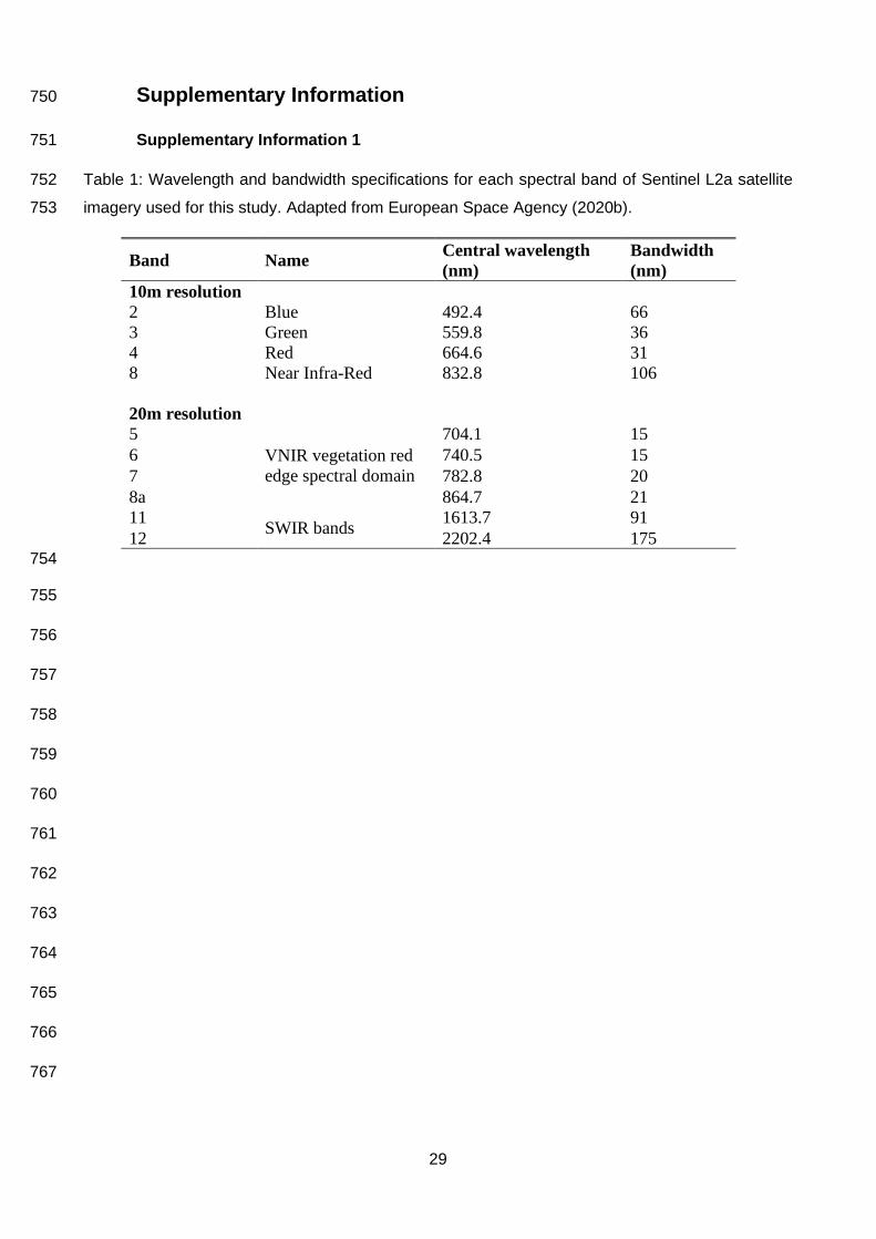
Supplementary Information 750
Supplementary Information 1 751
Table 1: Wavelength and bandwidth specifications for each spectral band of Sentinel L2a satellite 752
imagery used for this study. Adapted from European Space Agency (2020b). 753
Band Name Central wavelength
(nm)
Bandwidth
(nm)
10m resolution
2 Blue 492.4 66
3 Green 559.8 36
4 Red 664.6 31
8 Near Infra-Red 832.8 106
20m resolution
5
VNIR vegetation red
edge spectral domain
704.1 15
6 740.5 15
7 782.8 20
8a 864.7 21
11 SWIR bands
1613.7 91
12 2202.4 175
754
755
756
757
758
759
760
761
762
763
764
765
766
767
30
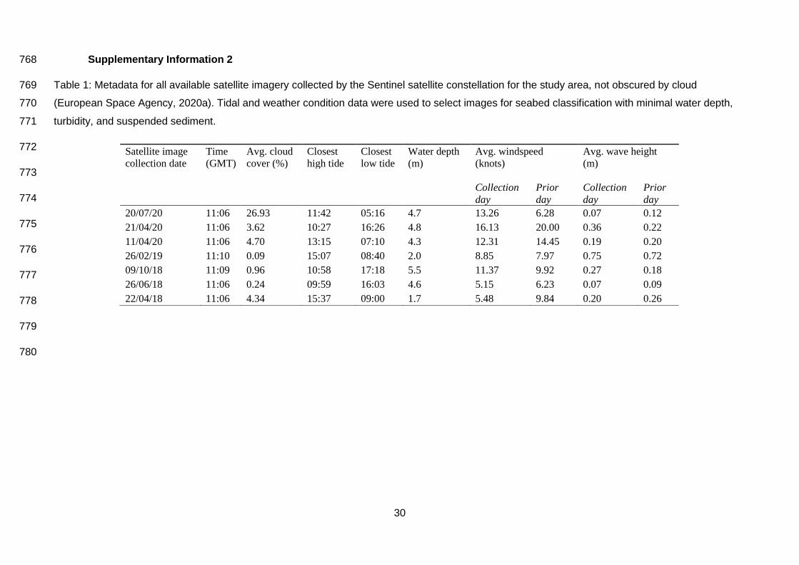
Supplementary Information 2 768
Table 1: Metadata for all available satellite imagery collected by the Sentinel satellite constellation for the study area, not obscured by cloud 769
(European Space Agency, 2020a). Tidal and weather condition data were used to select images for seabed classification with minimal water depth, 770
turbidity, and suspended sediment. 771
772
773
774
775
776
777
778
779
780
Satellite image
collection date
Time
(GMT)
Avg. cloud
cover (%)
Closest
high tide
Closest
low tide
Water depth
(m)
Avg. windspeed
(knots)
Avg. wave height
(m)
Collection
day
Prior
day
Collection
day
Prior
day
20/07/20 11:06 26.93 11:42 05:16 4.7 13.26 6.28 0.07 0.12
21/04/20 11:06 3.62 10:27 16:26 4.8 16.13 20.00 0.36 0.22
11/04/20 11:06 4.70 13:15 07:10 4.3 12.31 14.45 0.19 0.20
26/02/19 11:10 0.09 15:07 08:40 2.0 8.85 7.97 0.75 0.72
09/10/18 11:09 0.96 10:58 17:18 5.5 11.37 9.92 0.27 0.18
26/06/18 11:06 0.24 09:59 16:03 4.6 5.15 6.23 0.07 0.09
22/04/18 11:06 4.34 15:37 09:00 1.7 5.48 9.84 0.20 0.26
31
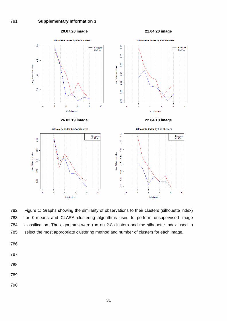
Supplementary Information 3 781
20.07.20 image 21.04.20 image
26.02.19 image 22.04.18 image
Figure 1: Graphs showing the similarity of observations to their clusters (silhouette index) 782
for K-means and CLARA clustering algorithms used to perform unsupervised image 783
classification. The algorithms were run on 2-8 clusters and the silhouette index used to 784
select the most appropriate clustering method and number of clusters for each image. 785
786
787
788
789
790
32
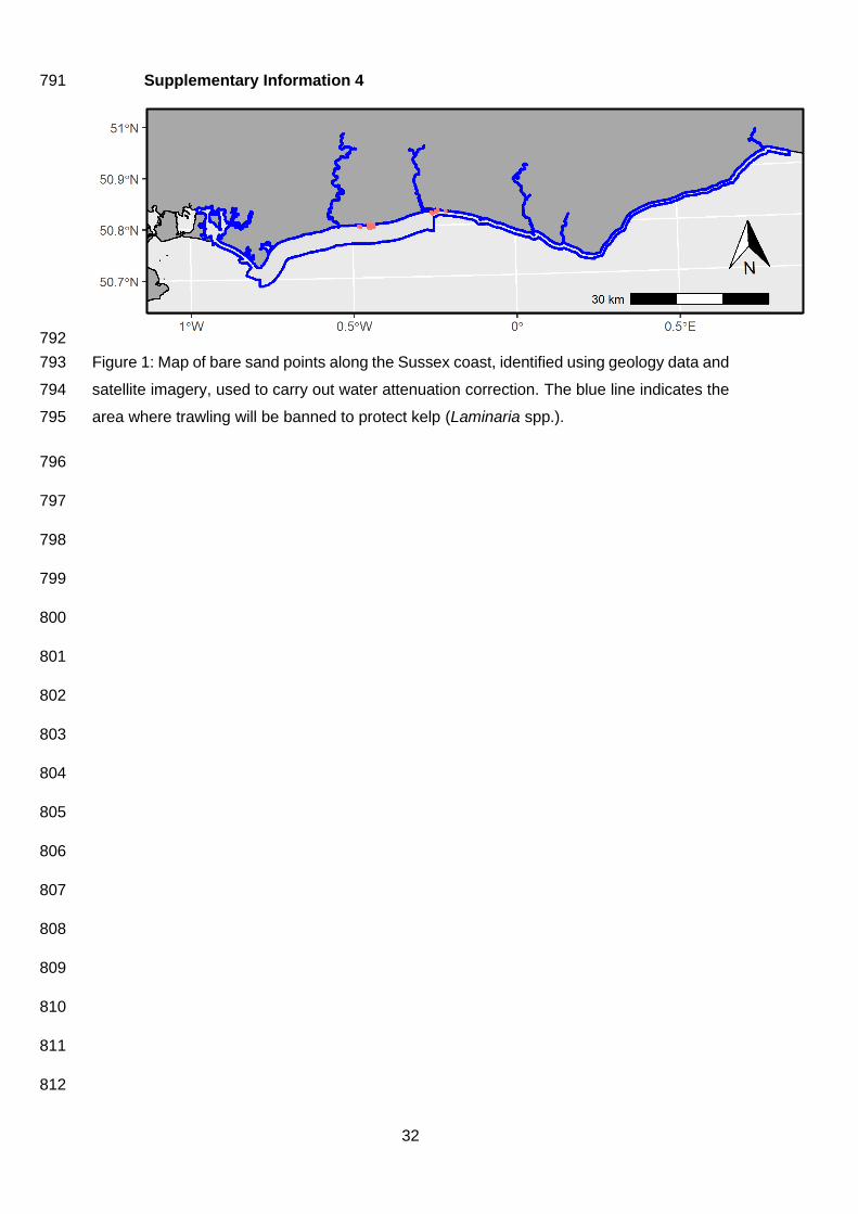
Supplementary Information 4 791
792
Figure 1: Map of bare sand points along the Sussex coast, identified using geology data and 793
satellite imagery, used to carry out water attenuation correction. The blue line indicates the 794
area where trawling will be banned to protect kelp (Laminaria spp.). 795
796
797
798
799
800
801
802
803
804
805
806
807
808
809
810
811
812

33
Supplementary Information 5 813
Table 1: Coefficients for multiple linear regressions showing the rate of light attenuation 814
through the water column (attenuation coefficients) at varying depths. Logged values for 815
each light band are taken as the response variables for each model, and depth as the 816
explanatory variable. 817
Log near infra-red band
Predictors Estimates CI p
(Intercept) 9.44 7.74 – 11.15 <0.001
Depth -0.85 -1.20 – -0.49 <0.001
Observations 20
R2 / R2 adjusted 0.58 / 0.56
818
Log red band
Predictors Estimates CI p
(Intercept) 9.69 8.61 – 10.78 <0.001
Depth -0.68 -0.90 – -0.45 <0.001
Observations 20
R2 / R2 adjusted 0.69 / 0.67
819
Log green band
Predictors Estimates CI p
(Intercept) 8.77 8.10 – 9.45 <0.001
Depth -0.36 -0.51 – -0.22 <0.001
Observations 20
R2 / R2 adjusted 0.62 / 0.60
820
Log blue band
Predictors Estimates CI p
(Intercept) 8.41 7.67 – 9.15 <0.001
Depth -0.35 -0.51 – -0.20 <0.001
Observations 20
R2 / R2 adjusted 0.57 / 0.54
34
Supplementary Information 6 821
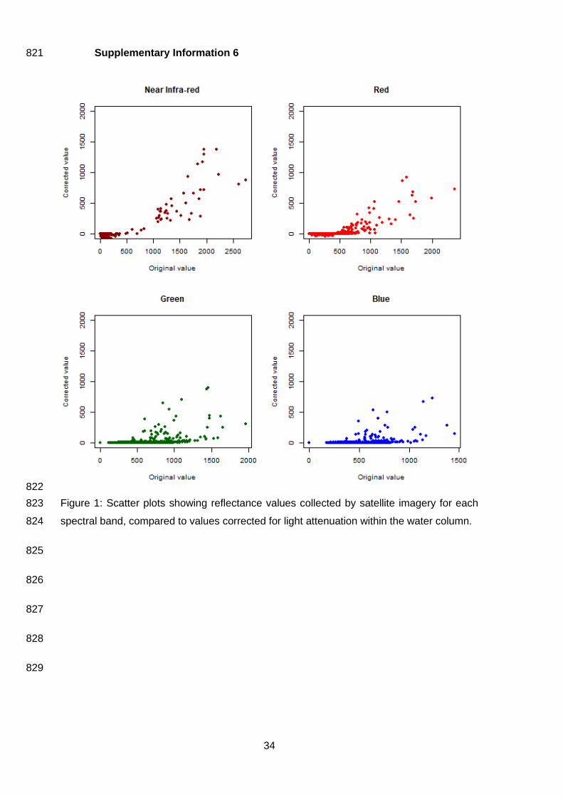
822
Figure 1: Scatter plots showing reflectance values collected by satellite imagery for each 823
spectral band, compared to values corrected for light attenuation within the water column. 824
825
826
827
828
829

35
Supplementary Information 7 830
Table 1: Pairwise comparisons of predicted habitat class (kelp presence/absence) between seabed sediment classes, using Mann-Whitney U test. 831
Adjusted p values using "fdr" control the false discovery rate (expected proportion of false positives), less stringently than family-wise error therefore 832
having a higher power for large datasets. 833
Gravelly
muddy
sand
Gravel Gravelly
sand
Muddy
sandy
gravel
Muddy
sand
Sandy
gravel
Sandy
mud
Slightly
gravelly
muddy
sand
Slightly
gravelly
sand
Slightly
gravelly
sandy
mud
Sand Rock
Gravel <0.001 - - - - - - - - - - -
Gravelly sand <0.001 <0.001 - - - - - - - - - -
Muddy sandy gravel 0.3203 <0.001 <0.001 - - - - - - - - -
Muddy sand <0.001 <0.001 <0.001 <0.001 - - - - - - - -
Sandy gravel <0.001 <0.001 <0.001 <0.001 <0.001 - - - - - - -
Sandy mud <0.001 <0.001 <0.001 <0.001 <0.001 <0.001 - - - - - -
Slightly gravelly muddy sand <0.001 <0.001 <0.001 <0.001 <0.001 <0.001 <0.001 - - - - -
Slightly gravelly sand <0.001 <0.001 <0.001 <0.001 <0.001 <0.001 <0.001 <0.001 - - - -
Slightly gravelly sandy mud <0.001 <0.001 <0.001 <0.001 <0.001 <0.001 <0.001 <0.001 <0.001 - - -
Sand <0.001 <0.001 <0.001 <0.001 <0.001 <0.001 <0.001 <0.001 <0.001 <0.001 - -
Rock <0.001 <0.001 <0.001 <0.001 <0.001 <0.001 <0.01 <0.001 <0.001 <0.001 <0.001 -
Rock and sediment <0.001 <0.001 <0.001 <0.001 <0.001 <0.001 <0.001 <0.001 <0.001 0.21 <0.001 <0.001
834
835