The Analysis of Optical Properties of Nanoparticles Using ... · complex conjugate pole pairs, the...

Vol. 5(17) Oct. 2015, PP. 2507-2516

2507

Article History:

IJMEC DOI: 649123/10168 Received Date: Jan. 06, 2015 Accepted Date: Sep. 04, 2015 Available Online: Sep. 19, 2015

The Analysis of Optical Properties of Nanoparticles Using General Model

Akbar Asadi

Department of Physics, Maritime University of Imam Khomaini, Nowshahr, Iran

*Corresponding Author's E-mail: [email protected]

Abstract

n this paper, a dispersion model, referred to as the general model, is proposed for modeling

dispersive materials in wide wavelength range using the Finite-Difference Time-Domain (FDTD)

method. A parameter estimation method is introduced for the general model to fit material

permittivity functions fast and accurately. The improved FDTD method with the general model is

implemented and verified in simulation of the nanowires. The scattering cross-section (SCS) spectrum

characteristics of different nanoparticles are systematically studied by employing the implemented

method. The optical properties such as SCS and electric field enhancement of nano-ellipses are

simulated by the accelerated 2D FDTD method and those of nano-ellipsoids are simulated by the

accelerated 3D FDTD method.

Keywords: FDTD, general model, nanoparticles.

1. Introduction

Dispersive materials, such as metals, are widely used in optical devices. The Finite-Difference

Time-Domain (FDTD) method [1] is one of the most common choices for simulating such devices in a

wide frequency range. One of the most important advantages of the FDTD method is that the

broadband response can be accurately obtained in only one simulation run [2]. Several simple

dispersion models, such as multi-pole Debye, Drude, and Lorentz models, have been widely adopted

for modeling dispersive materials using the FDTD method [3]. To fit permittivity function of a given

material accurately in a wide frequency range, a large number of poles are required in these models.

Rakic and Djurisic used the Durde model with up to five Lorentzian terms to fit the permittivity

functions of eleven metals [4]. Hao and Nordlander proposed an improved model consisting of four

Lorentzian terms to fit dielectric data of gold [5]. All the proposed multi-pole models archived good fit

to the measure data. However, using a dispersion model with a large number of poles not only requires

a lot of efforts for modal parameter estimation but also dramatically increases the memory and

computational costs of the FDTD method [6]. Han, Dutton and Fan proposed a complex-conjugate

pole-residue pair model and implemented it in the FDTD method to increase the modeling efficiency

[7, 8]. However, these authors did not propose an efficient method for the parameters estimation. The

FDTD formulation for dispersive materials are developed using the Z transform and frequency

approximation methods [9]. In this paper, a dispersion model, referred to as the general model with a

parameter estimation method is proposed for the simulation of optical properties of arbitrary linear

dispersive media over a wide wavelength range. The conventional Debye, Drude and Lorentz models

are derivable from this general model. The time domain properties of the proposed model are

analyzed. It is demonstrated that the model can fit the relative permittivity data of a material accurately

and efficiently in a wide wavelength range and the parameters of this model can be estimated requiring

I

mailto:[email protected]

Akbar Asadi / Vol. 5(17) Oct. 2015, pp. 2507-2516 IJMEC DOI: 649123/10168

2508

International Journal of Mechatronics, Electrical and Computer Technology (IJMEC)

Universal Scientific Organization, www.aeuso.org PISSN: 2411-6173, EISSN: 2305-0543

no initial guess. The general model is implemented in the FDTD method as a powerful and

computationally efficient tool for simulating nanoparticles of dispersive materials in a wide

wavelength range of light. By employing this model, a systematic study of the optical properties of

different nanoparticles gives a good reference for designs of optical devices utilizing the cross-section

spectra characteristics of nanoparticles.

2. General Dispersion Model Assuming the time harmonic dependence, , the general model is proposed to describe the

dispersive material’s relative permittivity expressed by the fraction form as

( ) ∑

( )

∑ ( )

(1a)

Where , are real numbers. The fraction form is the ratio of two polynomials ∑ ( ) and

∑ ( ) , where the highest order of the denominator is the same as that of the numerator. To be

conveniently adopted by the FDTD method, the general model is represented by its partial fraction

expansion described by

( ) ∑ ( ) (1b)

Where

( ) ∑

- ( )

∑ ( )

(2a)

Where , are real numbers.

Or, ( )

{

∑

( )

(2b)

Where , and ; are the direct coefficient, residue, and pole, respectively. The partial fraction

term ( ),is the frequency domain susceptibility function. It has three forms depending on the

properties of the pole : 1) a real fraction term with a real residue and a real pole, when is a real

number; 2) two complex fraction terms consist of complex conjugate residue and pole pairs, when

is a complex number; and 3) a summation of fraction terms which contains high order (>1) of j,

when is a multiple root of the denominator ∑ ( ) It is observed that the third expression

of should be avoided in the parameter estimation procedure because the high order (the order of

jis higher than one) partial fraction terms make it difficult to implement this model in the FDTD

method. If there are real poles and complex conjugate pole pairs, the upper bound of the

summation in equation (2) is L , and the total pole number is N 2

Table 1 shows relationships of the general model with other dispersion models.

It shows that Debye, Drude, and Lorentz models are all special cases of general model with specified

parameters. The general model treats the Debye, Drude, and Lorentz materials in a unified.


2509



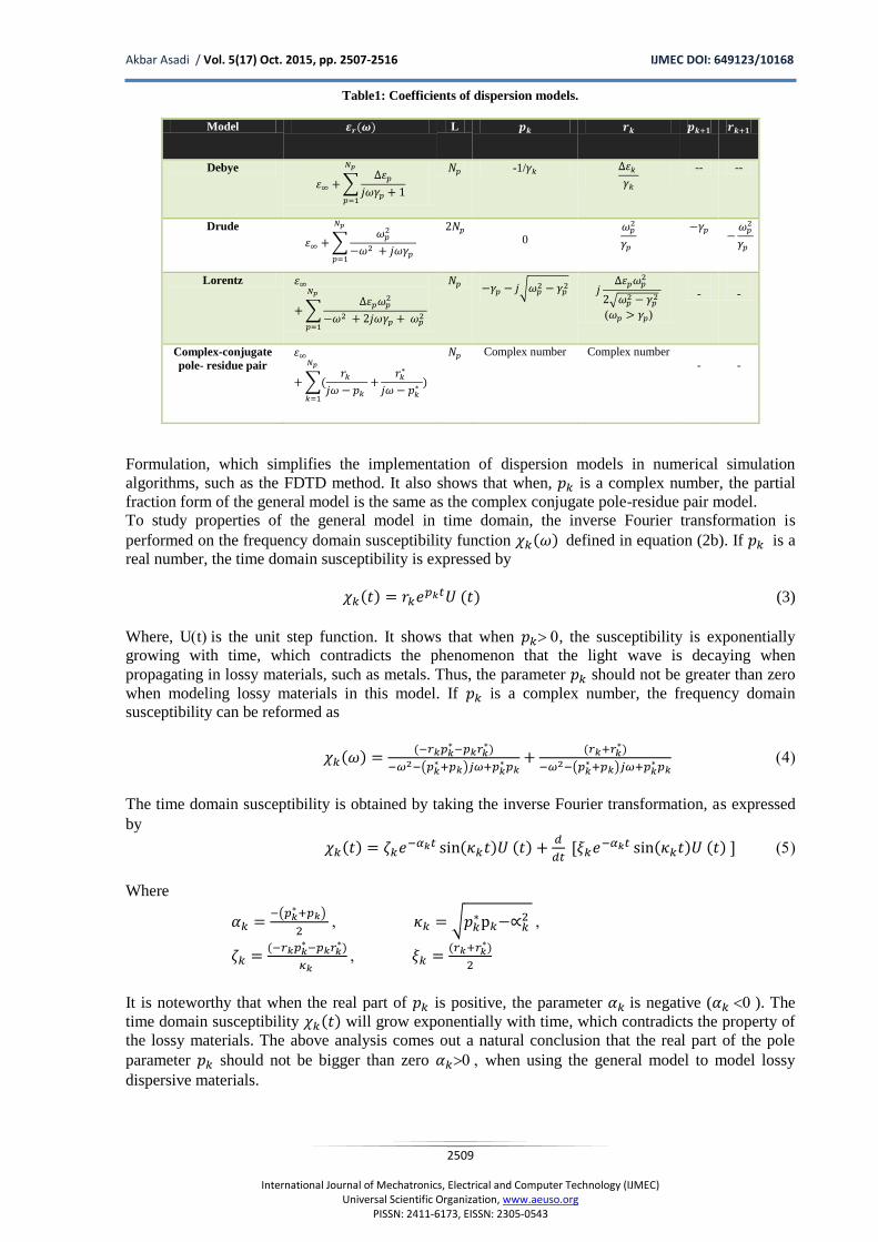
Table1: Coefficients of dispersion models.

Model ( ) L

Debye

∑

-1/

-- --

Drude

∑

0

Lorentz

∑

√

√

( )

-

-

Complex-conjugate

pole- residue pair

∑(

)

Complex number Complex number

-

-

Formulation, which simplifies the implementation of dispersion models in numerical simulation

algorithms, such as the FDTD method. It also shows that when, is a complex number, the partial

fraction form of the general model is the same as the complex conjugate pole-residue pair model.

To study properties of the general model in time domain, the inverse Fourier transformation is

performed on the frequency domain susceptibility function ( ) defined in equation (2b). If is a

real number, the time domain susceptibility is expressed by

( ) ( ) (3)

Where, Utis the unit step function. It shows that when , the susceptibility is exponentially

growing with time, which contradicts the phenomenon that the light wave is decaying when

propagating in lossy materials, such as metals. Thus, the parameter should not be greater than zero

when modeling lossy materials in this model. If is a complex number, the frequency domain

susceptibility can be reformed as

( ) (

)

( )

( )

( )

The time domain susceptibility is obtained by taking the inverse Fourier transformation, as expressed

by

( ) ( ) ( )

( ) ( )

Where

(

)

√

(

)

( )

It is noteworthy that when the real part of is positive, the parameter is negative ( ). The

time domain susceptibility ( ) will grow exponentially with time, which contradicts the property of

the lossy materials. The above analysis comes out a natural conclusion that the real part of the pole

parameter should not be bigger than zero when using the general model to model lossy

dispersive materials.


2510



The general model can be easily and efficiently implemented in the FDTD method with an auxiliary

differential equation (ADE) scheme. In Maxwell’s equations, Ampere’s law in frequency domain is

expressed by

∑

(6)

Where, is the polarization current related with each term in the summation of the general model,

defined by

{

(

)

(7)

As mentioned previously, the multiple-root should be avoided in the parameter estimation

procedure, so that it would not be concerned with the difficult implementation of polarization current

in the multiple-root case. If is real, is also real. Then the time-domain polarization current is

real and given by

(8)

If is complex, is also complex. The time-domain polarization current has two parts and , corresponding to the two complex poles in equation (7). The two polarization currents are all complex

and given by

(9)

(10)

Because Etis real, if the initial values for the two polarizations current are the same, the two parts

are mutual complex conjugate, i.e.

[7]. Only one complex equation, either equation (9) or (10),

needs to be computed in the FDTD calculation. In the following derivation, equation (9) is employed.

Therefore, when is complex, the real part of the time domain polarization current is Re

[ ( ) =2 Re ( ) .By applying the inverse Fourier transform on both sides of equation(6), the time

domain Ampere’s curl equation is obtained as

∑ (

) (11)

Where m 1 if is real; m 2 if is complex. The time domain polarization current equation and

Ampere’s curl equation are combined together and discretized in the explicit FDTD scheme, yielding

(∑

(

)

) (12)

(

) (13)

Where


2511



{

∑ ( )

∑ ( )

∑ ( )

( )

The discretization of the magnetic field is the same as it is in the standard FDTD algorithm

[10]. This is an efficient implementation of the general model in the FDTD method. With the same

number of poles, the general model takes no additional memory and computational costs for updating

the auxiliary equations of the polarization currents compared with the conventional dispersion models

such as multi-pole Lorentz-Drude model. However, the general model offers more degrees of freedom

in fitting a permittivity function in the parameter estimation process. Thus, the implementation of the

general model in the FDTD method is far more computationally efficient compared to those of

Lorentz-Drude model. The general model is an analytical function that describes the relative

permittivity of a dispersive material. To fit a given relative permittivity curve accurately and quickly, a

parameter estimation procedure is highly demanded in obtaining a good initial guess for the starting

point and locating a good approximation to the global optimum.

The advantage of the fraction form of the general model in equation (1a) lies in the fact that a very

good initial guess of parameters and can be quickly obtained using the rational approximation

method [11, 12]. After that, the initial values of the residues , poles , and direct coefficient

are obtained from the parameters and by converting the general model from the rational

fraction form to the partial fraction form. Finally, the initial valuesare employed in a simulated

annealing algorithm [13] to find the optimized values of parameters; , and . The high

efficiency of the general model is demonstrated in modeling metal materials Au (gold in a wide range

of wavelength from 400 to 1100 nm)The measured relative permittivity of these three metals [14] is

fitted using four dispersion models: the 4-pole Lorentz-Drude model (1 Drude pole pair and 1 Lorentz

pole pair), the 6-pole Lorentz-Drude model (1 Drude pole pair and 2 Lorentz pole pairs), the general

model with 4 poles, and the general model with 6 poles. The Lorentz-Drude model is expressed in the

equation:

( )

∑

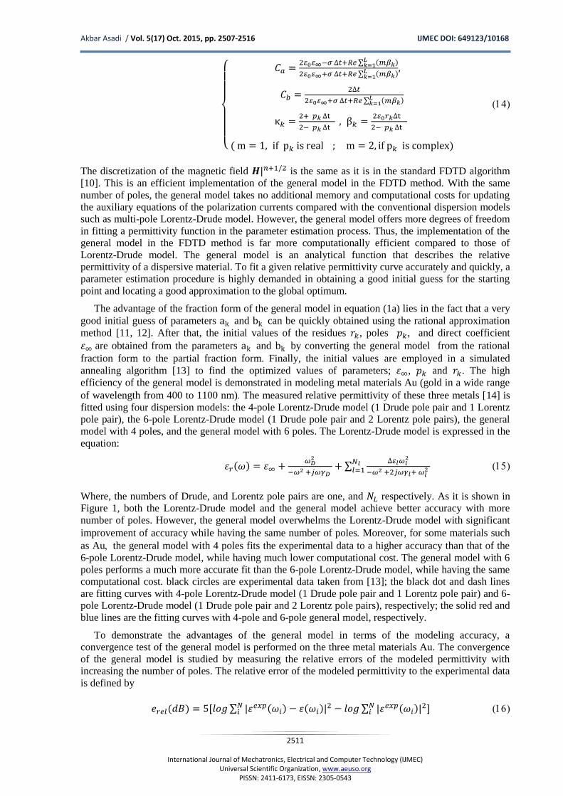
Where, the numbers of Drude, and Lorentz pole pairs are one, and respectively. As it is shown in

Figure 1, both the Lorentz-Drude model and the general model achieve better accuracy with more

number of poles. However, the general model overwhelms the Lorentz-Drude model with significant

improvement of accuracy while having the same number of polesMoreover, for some materials such

as Authe general model with 4 poles fits the experimental data to a higher accuracy than that of the

6-pole Lorentz-Drude model, while having much lower computational cost. The general model with 6

poles performs a much more accurate fit than the 6-pole Lorentz-Drude model, while having the same

computational cost. black circles are experimental data taken from [13]; the black dot and dash lines

are fitting curves with 4-pole Lorentz-Drude model (1 Drude pole pair and 1 Lorentz pole pair) and 6-

pole Lorentz-Drude model (1 Drude pole pair and 2 Lorentz pole pairs), respectively; the solid red and

blue lines are the fitting curves with 4-pole and 6-pole general model, respectively.

To demonstrate the advantages of the general model in terms of the modeling accuracy, a

convergence test of the general model is performed on the three metal materials Au. The convergence

of the general model is studied by measuring the relative errors of the modeled permittivity with

increasing the number of poles. The relative error of the modeled permittivity to the experimental data

is defined by

( ) ∑ ( ) ( )

∑ ( )


2512



Figure 1: (a) Real and (b) imaginary parts of the permittivity function of Au.

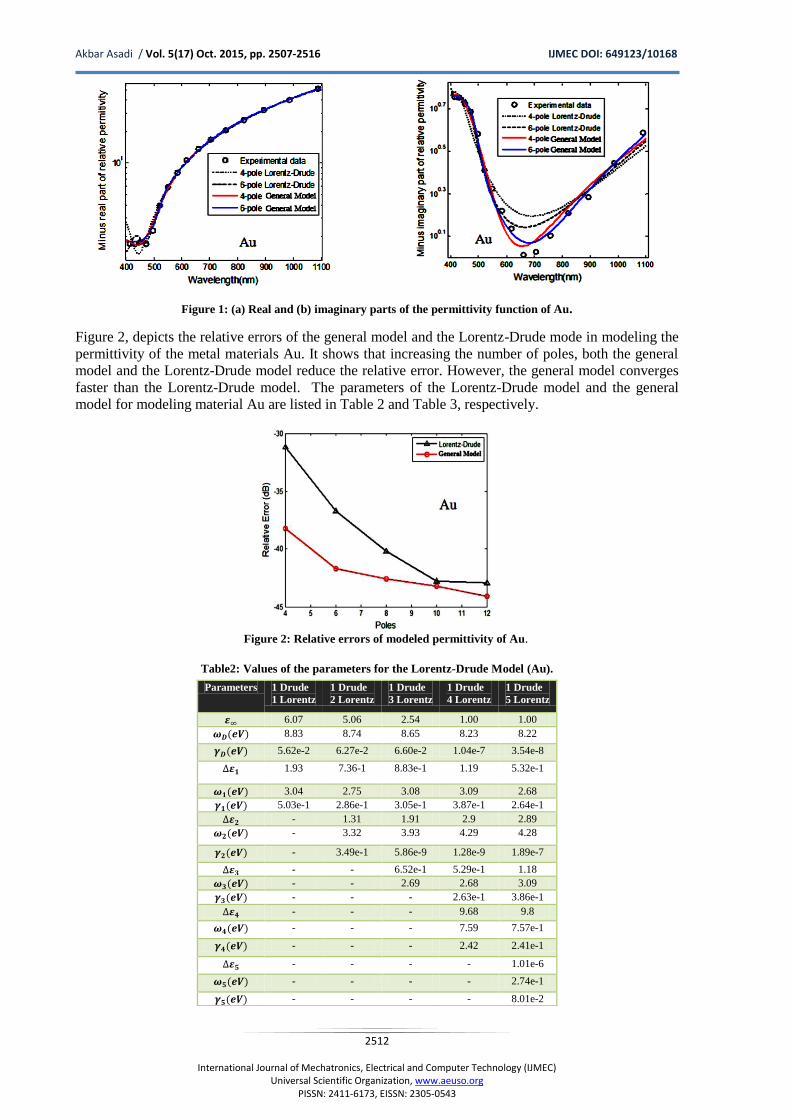
Figure 2, depicts the relative errors of the general model and the Lorentz-Drude mode in modeling the

permittivity of the metal materials Au. It shows that increasing the number of poles, both the general

model and the Lorentz-Drude model reduce the relative error. However, the general model converges

faster than the Lorentz-Drude model. The parameters of the Lorentz-Drude model and the general

model for modeling material Au are listed in Table 2 and Table 3, respectively.

Figure 2: Relative errors of modeled permittivity of Au.

Table2: Values of the parameters for the Lorentz-Drude Model (Au).

Parameters 1 Drude

1 Lorentz

1 Drude

2 Lorentz

1 Drude

3 Lorentz

1 Drude

4 Lorentz

1 Drude

5 Lorentz

6.07 5.06 2.54 1.00 1.00

( ) 8.83 8.74 8.65 8.23 8.22

( ) 5.62e-2 6.27e-2 6.60e-2 1.04e-7 3.54e-8

1.93 7.36-1 8.83e-1 1.19 5.32e-1

( ) 3.04 2.75 3.08 3.09 2.68

( ) 5.03e-1 2.86e-1 3.05e-1 3.87e-1 2.64e-1

- 1.31 1.91 2.9 2.89

( ) - 3.32 3.93 4.29 4.28

( ) - 3.49e-1 5.86e-9 1.28e-9 1.89e-7

- - 6.52e-1 5.29e-1 1.18

( ) - - 2.69 2.68 3.09

( ) - - - 2.63e-1 3.86e-1

- - - 9.68 9.8

( ) - - - 7.59 7.57e-1

( ) - - - 2.42 2.41e-1

- - - - 1.01e-6

( ) - - - - 2.74e-1

( ) - - - - 8.01e-2


2513



Table3: Values of the parameters for the General Model (Au).

Parameters 4-pole

General Model6-pole

General Model

Parameters 4-pole

General Model6-pole

General Model

2.99 1.00 ( ) -6.81e-1-2.6i -2.33e-1+2.52i

( ) -1.75e-2 -1.08e-2i -2.36e-2-8.55e-2i ( ) 3.7-1.67i 3.87e-1-3.14e-2i

( ) 1.46+3.4e+3i 1.53+402e+2 ( ) - -1.19-2.39i

( ) -1.75e-2+1.08e-2i -2.35e-2+8.65e-2i ( ) - 7.246+1.796e-1i

( ) 1.46-3.4e+3i 1.53-4.2e+2i ( ) - -1.186+2.390i

( ) -6.8e-1-2.6i -2.33e-1-2.52i ( ) - 7.246-1.796e-1i

( ) 3.69+1.67i 3.87e-1+3.14e-2i

3. Numerical Simulations

In this section, the general model is employed for modeling material properties of metal

nanoparticles in the light wave range with the FDTD method. It improves the accuracy of material

modeling while does not increase the computing cost of the FDTD method. The optical properties

such as scattering cross-section and electric field enhancement of nano-ellipses are simulated by the

accelerated 2D FDTD method and those of nano-ellipsoids are simulated by the accelerated 3D FDTD

method. The parameters employed for modeling the gold material with the general model in the FDTD

method are similar to what is listed in Table 3. 6 poles are used in the general model for all the

simulations.

3.1 Simulation of Nano-ellipsoid

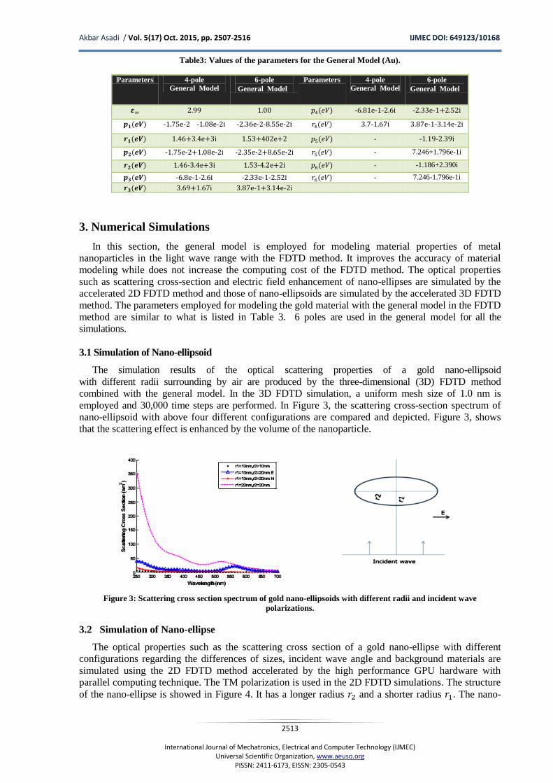
The simulation results of the optical scattering properties of a gold nano-ellipsoid

with different radii surrounding by air are produced by the three-dimensional (3D) FDTD method

combined with the general model. In the 3D FDTD simulation, a uniform mesh size of 1.0 nm is

employed and 30,000 time steps are performed. In Figure 3, the scattering cross-section spectrum of

nano-ellipsoid with above four different configurations are compared and depicted. Figure 3, shows

that the scattering effect is enhanced by the volume of the nanoparticle.

Figure 3: Scattering cross section spectrum of gold nano-ellipsoids with different radii and incident wave

polarizations.

3.2 Simulation of Nano-ellipse

The optical properties such as the scattering cross section of a gold nano-ellipse with different

configurations regarding the differences of sizes, incident wave angle and background materials are

simulated using the 2D FDTD method accelerated by the high performance GPU hardware with

parallel computing technique. The TM polarization is used in the 2D FDTD simulations. The structure

of the nano-ellipse is showed in Figure 4. It has a longer radius and a shorter radius . The nano-


2514



ellipse is illuminated by an incident plane wave propagating toward it with an angle of alpha to the

axis. The optical properties of this particle are studied in three cases. In the first case, the nano-ellipse

with a longer radius and a shorter radius is surrounded by air. The plane

wave propagates toward it from different directions, which means the angle alpha changes to different

values. In the Figure 5a, scattering cross section increases when angle alpha varying from 0 degree to

90 degree. It shows that the peak of the scattering cross section increases when angle size changes

from 0 to 90 degrees. When the longer axis of the nano-ellipse aligns with electric field polarization

direction (alpha=90 degrees), the peaks reach the maximum. However, the peak positions in the

spectra do not change in the simulations.

Figure 4: Structure of a single nano-ellipse illuminated by an incident plane wave.

Figure 5: Scattering cross section spectrum of a nano-ellipse: a) with incident wave illuminating from different

directions, b) surrounded by different materials.

In the second case, the nano-ellipse has the same size as that in the first case and the electric field of

the incident wave is polarized to the direction in the radius axis (alpha=90 degrees). However,

different surrounded materials such as air (index=1.0), water (index=1.33), silica (index=1.42),

Polymethyl Methacrylate (index=1.49) and silicon (index=3.2) are used in the simulations. The

scattering cross sections are depicted in Figure 5b. It shows that peak of the scattering cross section

increase along with the increase of the background material refractive index. With the increase of the

background refractive index, the peak positions in the spectra will shift to the long wavelengths (red

shift).

3.3 Non-regular cross section

We study the variation of SCS due to the nanoparticle shape. We consider three simple shapes, namely

a rectangle, equilateral triangle, and right triangle. Figure 6, compares the SCS for these shapes. As it

is shown, changing the shape affects the SCS amplitude, the resonance shift and line width. It is worth

recalling the SCS dependence on the illumination direction which is actually stronger when the

symmetry of the particle is reduced.

3.4 Circular cross section

As the last test, the FDTD method is a rigorous numerical tool for simulating nanoparticle problems

by solving Maxwell’s equations accurately. However, it is extremely memory and time consuming


2515



when dealing with metal nanostructures in the wavelength range of light due to two reasons: 1) the

small feature size of the structure requires very fine meshes and time steps; and 2) the complicated

dispersion property dramatically increases the implementation complexity and computational cost.

Therefore, it is strongly desired to have a simulation tool, which can accurately model the wide band

dispersion properties, yet taking an affordable computation effort.

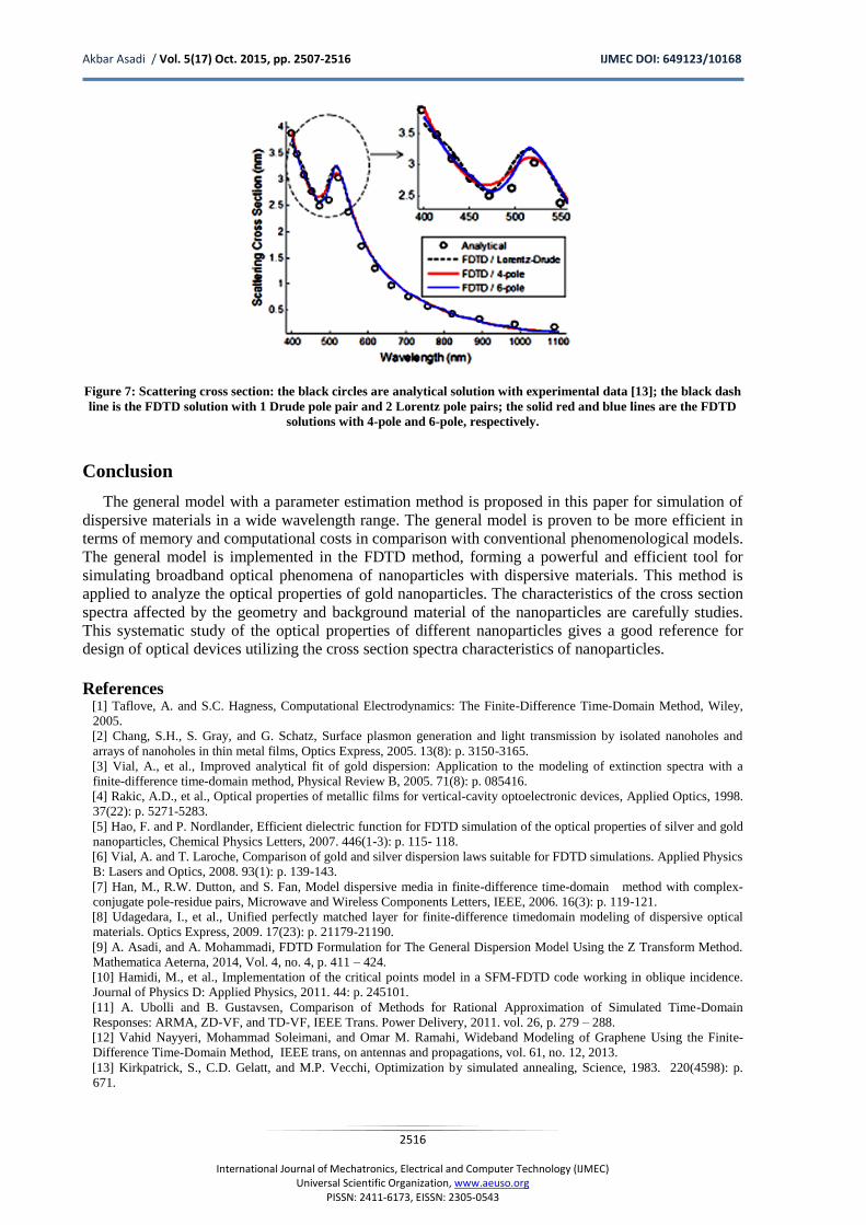
To exam the efficiency of the general model with different numbers of poles, the light wave

scattering phenomenon of an Au nanowire with 40 nm diameter surrounded by air is simulated by the

2D FDTD method using the general model in a wide wavelength range from 400 to 1100 nm. A

uniform mesh size of 0.5 nm is employed and 20,000 time steps are performed. Figure 7, shows the

cross section curves calculated using the analytical solution, the FDTD method with 1 Drude pole pair

and 2 Lorentz pole pairs (scheme 1), the FDTD method with the 4-pole general model (scheme 2), and

the FDTD method with the 6-pole general model (scheme 3), respectively.

Figure 6: The effect of cross section shape on SCS.

Table 4, lists the memory and computational costs of different FDTD schemes, as well as the relative

errors of the extinction cross-section compared with the analytical solution. It shows that compared

with the conventional Lorentz-Drude model, the FDTD method with the 4-pole General Model

achieves a smaller relative error while taking much less computational effort, and the FDTD method

with the 6-pole achieves even better accuracy yet maintaining a comparable computational cost.

Table4: Computational costs and relative errors of different FDTD schemes.

Scheme 3

(6 General Model

poles)

Scheme 2

(4 General Model poles)

Scheme 1

(1 Drude pole pair

and 2 Lorentz pole

pairs)

6.604 5.872 6.600 Memory

(mega-byte)

702.04 599.26 694.58 Computation time

(second)

-26.04 -25.31 -23.97 Relative error (dB)

(Extinction cross

section

It proves that the general model is more efficient in terms of memory and computational costs in

modeling dispersive materials in comparison with conventional models. It is a powerful and efficient

tool for simulating broadband optical phenomena of nanoparticles with dispersive materials.


2516



Figure 7: Scattering cross section: the black circles are analytical solution with experimental data [13]; the black dash

line is the FDTD solution with 1 Drude pole pair and 2 Lorentz pole pairs; the solid red and blue lines are the FDTD

solutions with 4-pole and 6-pole, respectively.

Conclusion

The general model with a parameter estimation method is proposed in this paper for simulation of

dispersive materials in a wide wavelength range. The general model is proven to be more efficient in

terms of memory and computational costs in comparison with conventional phenomenological models.

The general model is implemented in the FDTD method, forming a powerful and efficient tool for

simulating broadband optical phenomena of nanoparticles with dispersive materials. This method is

applied to analyze the optical properties of gold nanoparticles. The characteristics of the cross section

spectra affected by the geometry and background material of the nanoparticles are carefully studies.

This systematic study of the optical properties of different nanoparticles gives a good reference for

design of optical devices utilizing the cross section spectra characteristics of nanoparticles.

References [1] Taflove, A. and S.C. Hagness, Computational Electrodynamics: The Finite-Difference Time-Domain Method, Wiley,

2005.

[2] Chang, S.H., S. Gray, and G. Schatz, Surface plasmon generation and light transmission by isolated nanoholes and

arrays of nanoholes in thin metal films, Optics Express, 2005. 13(8): p. 3150-3165.

[3] Vial, A., et al., Improved analytical fit of gold dispersion: Application to the modeling of extinction spectra with a

finite-difference time-domain method, Physical Review B, 2005. 71(8): p. 085416.

[4] Rakic, A.D., et al., Optical properties of metallic films for vertical-cavity optoelectronic devices, Applied Optics, 1998.

37(22): p. 5271-5283.

[5] Hao, F. and P. Nordlander, Efficient dielectric function for FDTD simulation of the optical properties of silver and gold

nanoparticles, Chemical Physics Letters, 2007. 446(1-3): p. 115- 118.

[6] Vial, A. and T. Laroche, Comparison of gold and silver dispersion laws suitable for FDTD simulations. Applied Physics

B: Lasers and Optics, 2008. 93(1): p. 139-143.

[7] Han, M., R.W. Dutton, and S. Fan, Model dispersive media in finite-difference time-domain method with complex-

conjugate pole-residue pairs, Microwave and Wireless Components Letters, IEEE, 2006. 16(3): p. 119-121.

[8] Udagedara, I., et al., Unified perfectly matched layer for finite-difference timedomain modeling of dispersive optical

materials. Optics Express, 2009. 17(23): p. 21179-21190.

[9] A. Asadi, and A. Mohammadi, FDTD Formulation for The General Dispersion Model Using the Z Transform Method.

Mathematica Aeterna, 2014, Vol. 4, no. 4, p. 411 – 424.

[10] Hamidi, M., et al., Implementation of the critical points model in a SFM-FDTD code working in oblique incidence.

Journal of Physics D: Applied Physics, 2011. 44: p. 245101.

[11] A. Ubolli and B. Gustavsen, Comparison of Methods for Rational Approximation of Simulated Time-Domain

Responses: ARMA, ZD-VF, and TD-VF, IEEE Trans. Power Delivery, 2011. vol. 26, p. 279 – 288.

[12] Vahid Nayyeri, Mohammad Soleimani, and Omar M. Ramahi, Wideband Modeling of Graphene Using the Finite-

Difference Time-Domain Method, IEEE trans, on antennas and propagations, vol. 61, no. 12, 2013.

[13] Kirkpatrick, S., C.D. Gelatt, and M.P. Vecchi, Optimization by simulated annealing, Science, 1983. 220(4598): p.

671.

The Analysis of Optical Properties of Nanoparticles Using ... · complex conjugate pole pairs, the...

Documents

Transcript of The Analysis of Optical Properties of Nanoparticles Using ... · complex conjugate pole pairs, the...