THE ANALYSIS OF FACTORS AFFECTING CPO … ANALYSIS OF FACTORS AFFECTING CPO EXPORT PRICE OF...
13
European Journal of Accounting Auditing and Finance Research Vol.5, No.7, Pp.17-29, July 2017 ___Published by European Centre for Research Training and Development UK (www.eajournals.org) 17 THE ANALYSIS OF FACTORS AFFECTING CPO EXPORT PRICE OF INDONESIA Buyung 1 , Nur Syechalad 2 , Raja Masbar 2 , Muhammad Nasir 2 1 Doctoral Student of Economic Faculty of Syiah Kuala University 2 Lecturer of Economic Faculty of Syiah Kuala University ABSTRACT: This study aims to determine and analyze the influences of world crude oil price shocks, world soybean oil prices, world CPO prices, palm oil TBS prices and the exchange rate of rupiah/US dollar towards the transmission on CPO export prices of Indonesia. This study uses quantitative analysis model with the approach of vector autogression model (VAR) which includes three main analysis tools namely Granger causality test, impulse response function (IRF) and forecast error decomposition of variance (FEDV). The variables which are used in this research are world petroleum price, world soybean oil price, CPO price of Rotterdam, CPO export price of Indonesia, fresh fruit bunch price and real exchange rate (real exchange rate). From Granger Causality test result, The price transmission process takes place the plot as follows: world crude oil prices significantly influence the CPO price of world (Rotterdam) which will significantly influence the world soybean oil prices and so on have a significant influence on the value of the real exchange rate which will influence the price of fresh fruit bunches and ultimately have a significant influence on CPO price export of Indonesia. From the estimation result of VAR model, there are significant influences of world crude oil price shocks, world soybean oil prices, world CPO prices, palm oil TBS prices and rupiah/US dollar exchange rates simultaneously to the transmission on CPO export prices of Indonesia. Based on analysis of Impulse response and variance decomposition, in the first period, one hundred percent average variability of CPO export price growth is significantly explained by the average growth of CPO export prices itself. In the subsequent period, the average variability of CPO export price growth is significantly explained by the average growth of CPO export price itself as well as other variables. KEYWORDS: Petroleum Price, Soybean Oil Price, CPO export price, TBS, Real Exchange Rate, VAR, Granger causality, impulse response function, variance decomposition, Price Transmission INTRODUCTION Crude palm oil (CPO) is one of the alternative energy which is used as a substitute for petroleum, biodiesel energy. This will certainly influence the demand for world CPO. The good prospect in world trade is a source of foreign exchange for the government. Since 1984, palm oil exports of Indonesia have stabilized and continue to increase over the next few years. CPO production of Indonesia in 2015 reaches 32.5 million tons with export volume reaching 26.4 million tons with export value of US $ 18.6 billion (See Table 1). Fluctuations in CPO export prices will influence the prices at producer level and will ultimately influence CPO offerings. This price transmission will continue to influence the price of TBS at farmer level. In an era of increasingly open world trade, the fluctuations in CPO prices in
Transcript of THE ANALYSIS OF FACTORS AFFECTING CPO … ANALYSIS OF FACTORS AFFECTING CPO EXPORT PRICE OF...
European Journal of Accounting Auditing and Finance Research
Vol.5, No.7, Pp.17-29, July 2017
___Published by European Centre for Research Training and Development UK (www.eajournals.org)
17
THE ANALYSIS OF FACTORS AFFECTING CPO EXPORT PRICE OF
INDONESIA
Buyung1, Nur Syechalad2, Raja Masbar2, Muhammad Nasir2
1Doctoral Student of Economic Faculty of Syiah Kuala University 2Lecturer of Economic Faculty of Syiah Kuala University
ABSTRACT: This study aims to determine and analyze the influences of world crude oil
price shocks, world soybean oil prices, world CPO prices, palm oil TBS prices and the
exchange rate of rupiah/US dollar towards the transmission on CPO export prices of
Indonesia. This study uses quantitative analysis model with the approach of vector
autogression model (VAR) which includes three main analysis tools namely Granger causality
test, impulse response function (IRF) and forecast error decomposition of variance (FEDV).
The variables which are used in this research are world petroleum price, world soybean oil
price, CPO price of Rotterdam, CPO export price of Indonesia, fresh fruit bunch price and
real exchange rate (real exchange rate). From Granger Causality test result, The price
transmission process takes place the plot as follows: world crude oil prices significantly
influence the CPO price of world (Rotterdam) which will significantly influence the world
soybean oil prices and so on have a significant influence on the value of the real exchange rate
which will influence the price of fresh fruit bunches and ultimately have a significant influence
on CPO price export of Indonesia. From the estimation result of VAR model, there are
significant influences of world crude oil price shocks, world soybean oil prices, world CPO
prices, palm oil TBS prices and rupiah/US dollar exchange rates simultaneously to the
transmission on CPO export prices of Indonesia. Based on analysis of Impulse response and
variance decomposition, in the first period, one hundred percent average variability of CPO
export price growth is significantly explained by the average growth of CPO export prices
itself. In the subsequent period, the average variability of CPO export price growth is
significantly explained by the average growth of CPO export price itself as well as other
variables.
KEYWORDS: Petroleum Price, Soybean Oil Price, CPO export price, TBS, Real Exchange
Rate, VAR, Granger causality, impulse response function, variance decomposition, Price
Transmission
INTRODUCTION
Crude palm oil (CPO) is one of the alternative energy which is used as a substitute for
petroleum, biodiesel energy. This will certainly influence the demand for world CPO. The good
prospect in world trade is a source of foreign exchange for the government. Since 1984, palm
oil exports of Indonesia have stabilized and continue to increase over the next few years. CPO
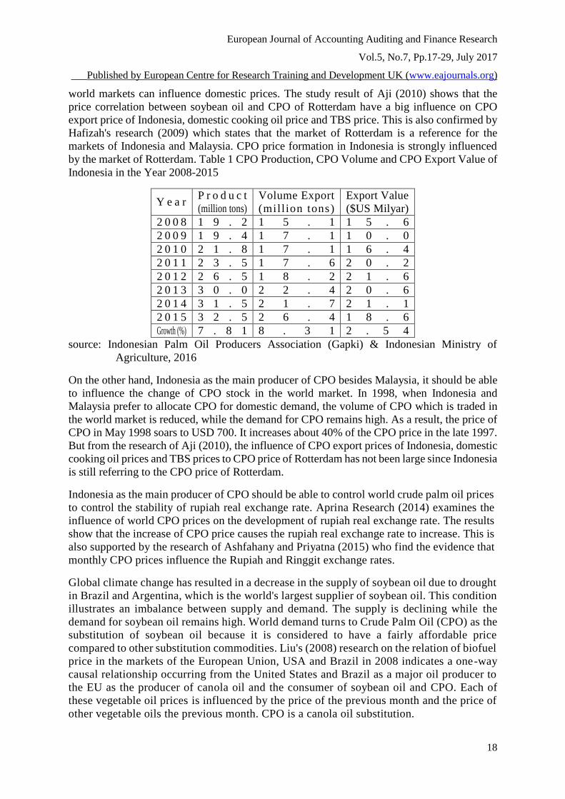
production of Indonesia in 2015 reaches 32.5 million tons with export volume reaching 26.4
million tons with export value of US $ 18.6 billion (See Table 1).
Fluctuations in CPO export prices will influence the prices at producer level and will ultimately
influence CPO offerings. This price transmission will continue to influence the price of TBS
at farmer level. In an era of increasingly open world trade, the fluctuations in CPO prices in
European Journal of Accounting Auditing and Finance Research
Vol.5, No.7, Pp.17-29, July 2017
___Published by European Centre for Research Training and Development UK (www.eajournals.org)
18
world markets can influence domestic prices. The study result of Aji (2010) shows that the
price correlation between soybean oil and CPO of Rotterdam have a big influence on CPO
export price of Indonesia, domestic cooking oil price and TBS price. This is also confirmed by
Hafizah's research (2009) which states that the market of Rotterdam is a reference for the
markets of Indonesia and Malaysia. CPO price formation in Indonesia is strongly influenced
by the market of Rotterdam. Table 1 CPO Production, CPO Volume and CPO Export Value of
Indonesia in the Year 2008-2015
Y e a r P r o d u c t
(million tons)
Volume Export
(mill ion tons)
Export Value
($US Milyar)
2 0 0 8 1 9 . 2 1 5 . 1 1 5 . 6
2 0 0 9 1 9 . 4 1 7 . 1 1 0 . 0
2 0 1 0 2 1 . 8 1 7 . 1 1 6 . 4
2 0 1 1 2 3 . 5 1 7 . 6 2 0 . 2
2 0 1 2 2 6 . 5 1 8 . 2 2 1 . 6
2 0 1 3 3 0 . 0 2 2 . 4 2 0 . 6
2 0 1 4 3 1 . 5 2 1 . 7 2 1 . 1
2 0 1 5 3 2 . 5 2 6 . 4 1 8 . 6
Growth (%) 7 . 8 1 8 . 3 1 2 . 5 4
source: Indonesian Palm Oil Producers Association (Gapki) & Indonesian Ministry of
Agriculture, 2016
On the other hand, Indonesia as the main producer of CPO besides Malaysia, it should be able
to influence the change of CPO stock in the world market. In 1998, when Indonesia and
Malaysia prefer to allocate CPO for domestic demand, the volume of CPO which is traded in
the world market is reduced, while the demand for CPO remains high. As a result, the price of
CPO in May 1998 soars to USD 700. It increases about 40% of the CPO price in the late 1997.
But from the research of Aji (2010), the influence of CPO export prices of Indonesia, domestic
cooking oil prices and TBS prices to CPO price of Rotterdam has not been large since Indonesia
is still referring to the CPO price of Rotterdam.
Indonesia as the main producer of CPO should be able to control world crude palm oil prices
to control the stability of rupiah real exchange rate. Aprina Research (2014) examines the
influence of world CPO prices on the development of rupiah real exchange rate. The results
show that the increase of CPO price causes the rupiah real exchange rate to increase. This is
also supported by the research of Ashfahany and Priyatna (2015) who find the evidence that
monthly CPO prices influence the Rupiah and Ringgit exchange rates.
Global climate change has resulted in a decrease in the supply of soybean oil due to drought
in Brazil and Argentina, which is the world's largest supplier of soybean oil. This condition
illustrates an imbalance between supply and demand. The supply is declining while the
demand for soybean oil remains high. World demand turns to Crude Palm Oil (CPO) as the
substitution of soybean oil because it is considered to have a fairly affordable price
compared to other substitution commodities. Liu's (2008) research on the relation of biofuel
price in the markets of the European Union, USA and Brazil in 2008 indicates a one-way
causal relationship occurring from the United States and Brazil as a major oil producer to
the EU as the producer of canola oil and the consumer of soybean oil and CPO. Each of
these vegetable oil prices is influenced by the price of the previous month and the price of
other vegetable oils the previous month. CPO is a canola oil substitution.
European Journal of Accounting Auditing and Finance Research
Vol.5, No.7, Pp.17-29, July 2017
___Published by European Centre for Research Training and Development UK (www.eajournals.org)
19
Increasing world demand for CPO causes CPO price developments tend to increase. The
sharp increase of CPO price has occurred since 2006, from USD400 per ton to USD1200
per ton in 2008 (Depperin 2009). This increase is related to the use of CPO as biofuel due
to petroleum prices increasing. There is a restriction of petroleum production by producer
countries causes the supply in the world market decline. Consequently, petroleum-
consuming countries are looking for alternative fuels for petroleum. Campiche, et al. (2007)
examines whether there is the incidence of agricultural commodity prices increase in
relation to the changes in the world's petroleum price increase in 2007. The variables which
are used in are petroleum prices, corn prices, sugar prices, soybean prices, soybean oil
prices and CPO prices. In period 2006-2007, it is only the price of soybean and corn which
are cointegrated with the price of petroleum. In period 2003-2006, the price of oil soybean
and CPO are negatively correlated with the price of petroleum.
The food crisis and the world energy crisis have had an impact on the competition for the use
of vegetable oils for food consumption and biofuel alternative fuels. Soybean oil, which
initially dominates the share of the world's vegetable oil consumption, its position is replaced
by CPO as a substitute, so that the decline in supply of soybean oil has an impact on CPO price
increase. Likewise, the limitation of petroleum production causes the price to increase, so that
the petroleum alternative replacement fuel which is relatively cheaper is seek. Therefore, as
one of the biofuel sources, the movement of CPO prices in the Rotterdam market is related to
the movement of petroleum prices.
CPO price of Rotterdam is the world reference price. As a result, the fluctuations in the CPO
market of Rotterdam can influence Indonesia as the world's largest producer of CPO. Similarly,
the expansion of land and increased production of oil palm TBS can also influence the price of
TBS at the farm level which will ultimately influence the continuity of domestic and export
CPO supply. The issue of CPO exports is related to the foreign trade aspect, the role of rupiah
exchange rate against US dollar will influence the CPO export price of Indonesia. Considering
the above, the purpose of this study is to know and analyze the influence of world crude oil
price shocks, world soybean oil price, world CPO price, palm oil TBS price and rupiah/US
dollar exchange rate against CPO export price of Indonesia.
DATA AND METHODOLOGY
The data which is used in this research is monthly data from year 2005-2014. The data
include the following variables:
PMBt = World petroleum price t month;
PMKt = World soybean oil price t month;
PROTt = CPO price of Rotterdam t month;
PINAt = CPO export price of Indonesia t month;
PTBSt = Fresh fruit bunches price t month;
KURSt = Exchange Rate (Rp/$ US) t month
European Journal of Accounting Auditing and Finance Research
Vol.5, No.7, Pp.17-29, July 2017
___Published by European Centre for Research Training and Development UK (www.eajournals.org)
20
The model of analysis in this study uses multivariate vector autogression (VAR) which is
generally stated as follows:
In which: Yt = Vector of endogenous variables in the model ie PMBt; PMKt; PROTt; PINAt;
PTBSt; KURSt; At = Parameter matrix and k= Order of VAR model.
The VAR model estimate procedure consists of: (1) unit root test which is used in many studies
is Augmented Dickey-Fuller (ADF) test model, (2) lag optimal length determination. This test
is useful to eliminate the problem of autocorrelation in the VAR system. Determination of lag
optimal length in this study mainly uses Akaike Information Criterion (AIC). Having obtained
the lag optimal length, it is necessary to test the stability of the VAR system. A VAR system
is said to be stable (stationary) if all of its roots have a smaller modulus than one and all are
located within a unit circle; (3) cointegration test which in this study using Johansen
cointegration test
The VAR model includes three main analytical tools: (1) Granger causality test is to see the
possible causality relationship between the variables to be used in the research model; (2)
Impulse Response Function (IRF) shows how the response of each endogenous variable at over
time to the shock of the variable itself and other endogenous variables. IRF results are very
sensitive to the ordering of variables that are used in the calculations which in this study is
based on cholesky factorization; (3) Forecast Error Decomposition of Variance (FEDV) is
conducted to provide information on how the dynamic relationship between variables which
are analyzed. In addition, FEVD is done to see how big the influence of random shock of a
particular variable to endogenous variables. FEVD produces information about the relative
importance of each random innovation (random innovation structural disturbance) or how
strongly the composition of a particular variable role over another.
RESULTS AND DISCUSSION
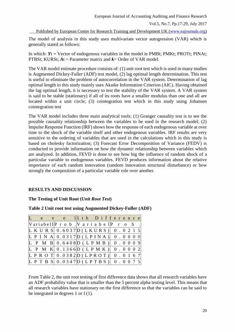
The Testing of Unit Root (Unit Root Test)
Table 2 Unit root test using Augmented Dickey-Fuller (ADF)
L e v e l 1 t h D i f f e r e n c e
V a r i a b e l l P r o b . V a r i a b e l P r o b .
L K U R S 0 . 6 0 3 7 D ( L K U R S ) 0 . 0 2 1 5
L P I N A 0 . 0 3 1 7 D ( L P I N A ) 0 . 0 0 0 0
L P M B 0 . 6 4 0 8 D ( L P M B ) 0 . 0 0 0 9
L P M K 0 . 1 3 6 6 D ( L P M K ) 0 . 0 0 0 2
L P R O T 0 . 0 3 8 2 D ( L P R O T ) 0 . 0 1 6 7
L P T B S 0 . 0 3 4 7 D ( L P T B S ) 0 . 0 0 7 5
From Table 2, the unit root testing of first difference data shows that all research variables have
an ADF probability value that is smaller than the 5 percent alpha testing level. This means that
all research variables have stationary on the first difference so that the variables can be said to
be integrated in degrees 1 or I (1).

European Journal of Accounting Auditing and Finance Research
Vol.5, No.7, Pp.17-29, July 2017
___Published by European Centre for Research Training and Development UK (www.eajournals.org)
21
Test of Cointegration
Based on Table 3, it can be seen that the Max-Eigen statistic value on r = 0 is smaller than the
critical value with Value Probability > 0.05. This result shows that among the six variables in
this study, there is no cointegration at the 5 percent significance level. The results of
cointegration indicate that among the six variables, they do not have a relationship of
stability/balance and the similarity of movement in the long term.
Table 3 Cointegration Testing Results
Hypothesized E i g e n v a l u e
M a x - E i g e n 0 . 0 5
P r o b . * * N o . o f C E ( s ) S t a t i s t i c Critical Value
N o n e * 0 . 2 3 4 9 8 8 3 1 . 0 7 2 1 8 4 0 . 0 7 7 5 7 0 . 3 5 6 3
A t m o s t 1 0 . 2 2 8 3 9 5 3 0 . 0 7 6 7 6 3 3 . 8 7 6 8 7 0 . 1 3 3 0
A t m o s t 2 0 . 1 3 7 7 4 3 1 7 . 1 9 1 4 7 2 7 . 5 8 4 3 4 0 . 5 6 3 5
A t m o s t 3 0 . 1 1 8 9 1 0 1 4 . 6 8 5 0 2 2 1 . 1 3 1 6 2 0 . 3 1 1 6
A t m o s t 4 0 . 0 6 0 3 6 2 7 . 2 2 2 2 7 3 1 4 . 2 6 4 6 0 0 . 4 6 3 2
A t m o s t 5 0 . 0 3 9 9 7 7 4 . 7 3 2 6 2 2 3 . 8 4 1 4 6 6 0 . 0 2 9 6
Max-eigenvalue test indicates no cointegration at the 0.05 level
* denotes rejection of the hypothesis at the 0.05 level
**MacKinnon-Haug-Michelis (1999) p-values
Determination of Lag Optimal
Based on Table 4, the criteria of LR, FPE and AIC are order 5 while the criteria of SC chooses
order 1 and HQ chooses order 2. Thus in this study the lag optimal length to be used is 5. The
implication of all research variables which are used in the equation influence each other not
only in the same period but those variables which are interrelated to five previous periods.
Table 4 Lag Optimal Length Based on Multiple Criteria
L a g L o g L L R F P E A I C S C H Q
0 1634.044 N A 1 . 2 3 e - 2 0 - 2 8 . 8 1 4 9 4 - 2 8 . 6 7 0 1 2 - 2 8 . 7 5 6 1 7
1 1973.459 6 3 6 . 7 7 9 3 5 . 7 4 e - 2 3 - 3 4 . 1 8 5 1 2 - 3 3 . 1 7 1 4 0 * - 3 3 . 7 7 3 7 6
2 2037.535 1 1 3 . 4 0 9 0 3 . 5 1 e - 2 3 - 3 4 . 6 8 2 0 4 - 3 2 . 7 9 9 4 2 - 3 3 . 9 1 8 0 9 *
3 2067.244 4 9 . 4 2 6 8 2 3 . 9 8 e - 2 3 - 3 4 . 5 7 0 6 9 - 3 1 . 8 1 9 1 7 - 3 3 . 4 5 4 1 5
4 2138.303 1 1 0 . 6 7 5 3 2 . 1 9 e - 2 3 - 3 5 . 1 9 1 2 0 - 3 1 . 5 7 0 7 7 - 3 3 . 7 2 2 0 7
5 2190.003 7 5 . 03 39 4 * 1 . 7 3 e - 2 3 * -35.46908* - 3 0 . 9 7 9 7 5 - 3 3 . 6 4 7 3 5
6 2223.624 4 5 . 2 2 4 3 8 1 . 9 3 e - 2 3 - 3 5 . 4 2 6 9 7 - 3 0 . 0 6 8 7 3 - 3 3 . 2 5 2 6 5
Description: * indicates lag order selected by the criterion
European Journal of Accounting Auditing and Finance Research
Vol.5, No.7, Pp.17-29, July 2017
___Published by European Centre for Research Training and Development UK (www.eajournals.org)
22
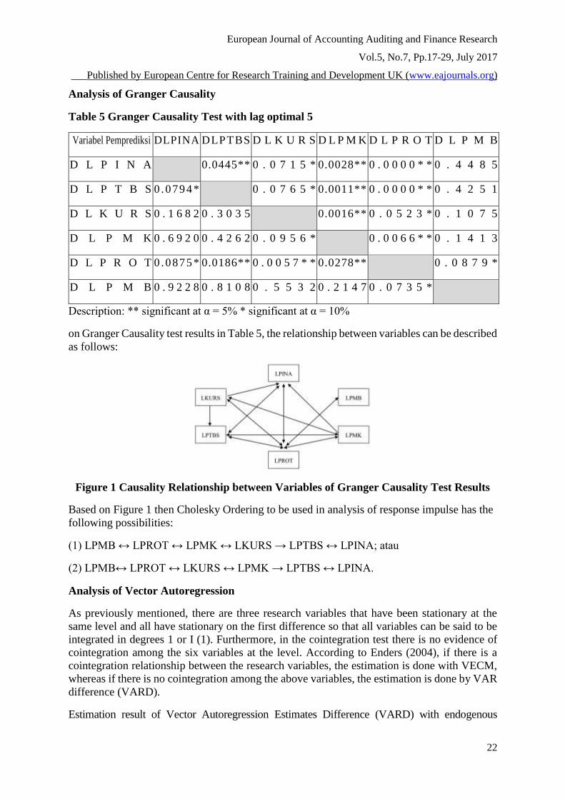
Analysis of Granger Causality
Table 5 Granger Causality Test with lag optimal 5
Variabel Pemprediksi DLPINA DLPTBS D L K U R S D L P M K D L P R O T D L P M B
D L P I N A 0.0445** 0 . 0 7 1 5 * 0.0028** 0 . 0 0 0 0 * * 0 . 4 4 8 5
D L P T B S 0 .0794 * 0 . 0 7 6 5 * 0.0011** 0 . 0 0 0 0 * * 0 . 4 2 5 1
D L K U R S 0 . 1 6 8 2 0 . 3 0 3 5 0.0016** 0 . 0 5 2 3 * 0 . 1 0 7 5
D L P M K 0 . 6 9 2 0 0 . 4 2 6 2 0 . 0 9 5 6 * 0 . 0 0 6 6 * * 0 . 1 4 1 3
D L P R O T 0 .0875 * 0.0186** 0 . 0 0 5 7 * * 0.0278** 0 . 0 8 7 9 *
D L P M B 0 . 9 2 2 8 0 . 8 1 0 8 0 . 5 5 3 2 0 . 2 1 4 7 0 . 0 7 3 5 *
Description: ** significant at α = 5% * significant at α = 10%
on Granger Causality test results in Table 5, the relationship between variables can be described
as follows:
Figure 1 Causality Relationship between Variables of Granger Causality Test Results
Based on Figure 1 then Cholesky Ordering to be used in analysis of response impulse has the
following possibilities:
(1) LPMB ↔ LPROT ↔ LPMK ↔ LKURS → LPTBS ↔ LPINA; atau
(2) LPMB↔ LPROT ↔ LKURS ↔ LPMK → LPTBS ↔ LPINA.
Analysis of Vector Autoregression
As previously mentioned, there are three research variables that have been stationary at the
same level and all have stationary on the first difference so that all variables can be said to be
integrated in degrees 1 or I (1). Furthermore, in the cointegration test there is no evidence of
cointegration among the six variables at the level. According to Enders (2004), if there is a
cointegration relationship between the research variables, the estimation is done with VECM,
whereas if there is no cointegration among the above variables, the estimation is done by VAR
difference (VARD).
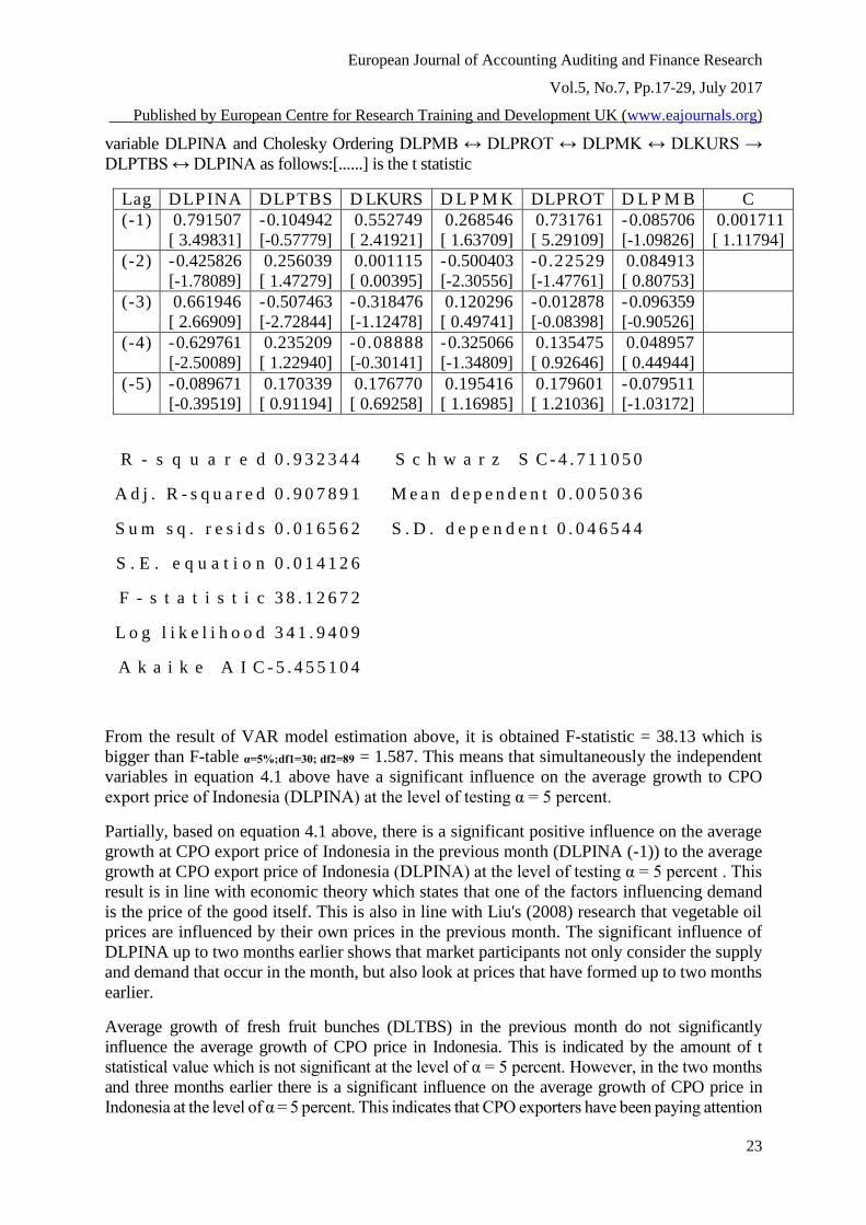
Estimation result of Vector Autoregression Estimates Difference (VARD) with endogenous
European Journal of Accounting Auditing and Finance Research
Vol.5, No.7, Pp.17-29, July 2017
___Published by European Centre for Research Training and Development UK (www.eajournals.org)
23
variable DLPINA and Cholesky Ordering DLPMB ↔ DLPROT ↔ DLPMK ↔ DLKURS →
DLPTBS ↔ DLPINA as follows:[......] is the t statistic
Lag DLPINA DLPTBS D LKURS D L P M K DLPROT D L P M B C
(-1) 0.791507 -0.104942 0.552749 0.268546 0.731761 -0.085706 0.001711
[ 3.49831] [-0.57779] [ 2.41921] [ 1.63709] [ 5.29109] [-1.09826] [ 1.11794]
(-2) -0.425826 0.256039 0.001115 -0.500403 -0.22529 0.084913
[-1.78089] [ 1.47279] [ 0.00395] [-2.30556] [-1.47761] [ 0.80753]
(-3) 0.661946 -0.507463 -0.318476 0.120296 -0.012878 -0.096359
[ 2.66909] [-2.72844] [-1.12478] [ 0.49741] [-0.08398] [-0.90526]
(-4) -0.629761 0.235209 -0.08888 -0.325066 0.135475 0.048957
[-2.50089] [ 1.22940] [-0.30141] [-1.34809] [ 0.92646] [ 0.44944]
(-5) -0.089671 0.170339 0.176770 0.195416 0.179601 -0.079511
[-0.39519] [ 0.91194] [ 0.69258] [ 1.16985] [ 1.21036] [-1.03172]
R - s q u a r e d 0 . 9 3 2 3 4 4 S c h w a r z S C - 4 . 7 1 1 0 5 0
A d j . R - s q u a r e d 0 . 9 0 7 8 9 1 M e a n d e p e n d e n t 0 . 0 0 5 0 3 6
S u m s q . r e s i d s 0 . 0 1 6 5 6 2 S . D . d e p e n d e n t 0 . 0 4 6 5 4 4
S . E . e q u a t i o n 0 . 0 1 4 1 2 6
F - s t a t i s t i c 3 8 . 1 2 6 7 2
L o g l i k e l i h o o d 3 4 1 . 9 4 0 9
A k a i k e A I C - 5 . 4 5 5 1 0 4
From the result of VAR model estimation above, it is obtained F-statistic = 38.13 which is
bigger than F-table α=5%;df1=30; df2=89 = 1.587. This means that simultaneously the independent
variables in equation 4.1 above have a significant influence on the average growth to CPO
export price of Indonesia (DLPINA) at the level of testing α = 5 percent.
Partially, based on equation 4.1 above, there is a significant positive influence on the average
growth at CPO export price of Indonesia in the previous month (DLPINA (-1)) to the average
growth at CPO export price of Indonesia (DLPINA) at the level of testing α = 5 percent . This
result is in line with economic theory which states that one of the factors influencing demand
is the price of the good itself. This is also in line with Liu's (2008) research that vegetable oil
prices are influenced by their own prices in the previous month. The significant influence of
DLPINA up to two months earlier shows that market participants not only consider the supply
and demand that occur in the month, but also look at prices that have formed up to two months
earlier.
Average growth of fresh fruit bunches (DLTBS) in the previous month do not significantly
influence the average growth of CPO price in Indonesia. This is indicated by the amount of t
statistical value which is not significant at the level of α = 5 percent. However, in the two months
and three months earlier there is a significant influence on the average growth of CPO price in
Indonesia at the level of α = 5 percent. This indicates that CPO exporters have been paying attention
European Journal of Accounting Auditing and Finance Research
Vol.5, No.7, Pp.17-29, July 2017
___Published by European Centre for Research Training and Development UK (www.eajournals.org)
24
to information on average growth of TBS prices up to three months earlier in exporting CPO.
Average growth of exchange rate (DLKURS) in the previous month significantly influence the
average growth of CPO price in Indonesia at the level of α = 5 percent. However, in the two
months to five months before the influence is not significant to the average growth of CPO
price in Indonesia at the level of α = 5 percent. This shows that CPO exporters have been paying
attention to the information on the average growth of previous exchange rate in the CPO export.
The average growth of soybean oil price (DLPMK) up to two months earlier has a significant
influence on average growth of CPO price in Indonesia. This is indicated by the significant t
statistical value at the level of α = 5 percent. In theory, the price of substitute goods is one of
the factors that influence the demand of a good. An item becomes a substitution of other goods
if it has the same function and or the same content. This is also in line with the research of
Purwanto (2002) that palm oil and soybean oil has substitutionary relationships. The research
result of Aji (2010) shows a positive but insignificant relationship between changes in soybean
oil price growth in the previous month and the change in CPO export price growth in Indonesia.
The average CPO price of Rotterdam in previous month has a positive and significant influence
on average growth of CPO price in Indonesia. This is indicated by the significant t statistical
value at the level of α = 5 percent. This is in line with the research of Hafizah's (2009) that
Rotterdam forward market is a reference market for Indonesian spot market. This means that
the changes in the market of Rotterdam will be followed by the market of Indonesia. The
significance of average growth to CPO export price in Indonesia is influenced by the average
growth of CPO price in Rotterdam in the previous month indicating that CPO exporters in
Indonesia in exporting CPO take into account the average growth of CPO price in Rotterdam
in the previous month. This is also reinforced by the research results of Aji (2010) indicates a
positive and significant relationship between average growth of CPO price in Rotterdam in the
previous month with the average growth of CPO export prices in Indonesia.
The average growth of petroleum price (DLPMB) up to previous five months has no
significant influence on the change of CPO price in Indonesia. This is indicated by the amount
of t statistical value which is not significant at the level of α = 5 percent. This finding is in
line with the research of Arianto (2008) ie between the CPO price and petroleum prices does
not occur consistency correlation. This finding is also corroborated by the research results of
Aji (2010) where the VECM estimation result indicates a negative but not significant
relationship between the changes in the growth of petroleum price in the previous month and
the change in the growth of CPO export price in Indonesia.
Analysis of Impulse Response
Analysis of impulse response is done to determine the sensivity of change influence in an
endogen variable to other endogen variable. The analysis results can show the current and
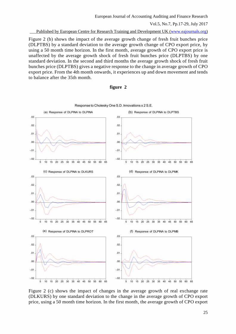
future impacts of a variable shock on other endogenous variables. Figure 2 (a) shows the impact
of the average growth change in CPO export price (DLPINA) by one standard deviation to the
average growth change in CPO export price, using a 60 month time horizon. In the first month,
average growth of CPO export rate is directly influenced positively by the average growth
shock of CPO export price itself (DLPINA) by one standard deviation. In the second month
until the fourth month the average growth shock of CPO export price (DLPINA) still responds
positively to the change in average growth of CPO export price. Starting from the fifth month
onwards, it experiences up and down movement and tends to balance after the 55th month.
European Journal of Accounting Auditing and Finance Research
Vol.5, No.7, Pp.17-29, July 2017
___Published by European Centre for Research Training and Development UK (www.eajournals.org)
25
Figure 2 (b) shows the impact of the average growth change of fresh fruit bunches price
(DLPTBS) by a standard deviation to the average growth change of CPO export price, by
using a 50 month time horizon. In the first month, average growth of CPO export price is
unaffected by the average growth shock of fresh fruit bunches price (DLPTBS) by one
standard deviation. In the second and third months the average growth shock of fresh fruit
bunches price (DLPTBS) gives a negative response to the change in average growth of CPO
export price. From the 4th month onwards, it experiences up and down movement and tends
to balance after the 35th month.
figure 2
Figure 2 (c) shows the impact of changes in the average growth of real exchange rate
(DLKURS) by one standard deviation to the change in the average growth of CPO export
price, using a 50 month time horizon. In the first month, the average growth of CPO export

European Journal of Accounting Auditing and Finance Research
Vol.5, No.7, Pp.17-29, July 2017
___Published by European Centre for Research Training and Development UK (www.eajournals.org)
26
prices is not influenced by the average growth shock of real exchange rate (DLKURS) by
one standard deviation. In the second month until the eighth month, the average growth
shock of real exchange rate (DLKURS) gives a positive response to the change in the
average growth of CPO export price. Beginning of the 9th month and onwards, it
experiences up and down movement and tends to balance after the 35th month.
Figure 2 (d) shows the impact to the change on the average growth of soybean oil price
(DLPMK) by one standard deviation to the change on the average growth of CPO export price,
by using a 50 month time horizon. In the first month, average growth of CPO export prices is
influenced by the average growth shock of soybean oil price (DLPMK) by one standard
deviation. However, in the second to sixth month the average growth shock of soybean oil price
(DLPMB) gives a positive response to the change in average growth of CPO export price
despite the decreasing response from the seventh month. Furthermore, the response shows a
movement up and down tends to balance after the 47th month. Between soybean oil and CPO
are substitute goods, where the increase in one good price can raise the other good price.
Theoretically this condition is in accordance with the criteria of substitution goods that is
proposed by Djojodipuro (1991). The results of this study are also in line with the research of
Yu et al. (2006) states that the vegetable oil price in the world market responds to shocks that
occur in one of the vegetable oil prices.
Figure 2 (e) shows the impact on change to average growth in CPO price of Rotterdam
(DLPROT) at one standard deviation to the change on average growth of CPO export price,
using a 50-month time horizon. In the first month, the average growth of CPO export price
is not influenced by the average growth on CPO price of Rotterdam (DLPROT) at one
standard deviation. But in the second until the eighth month, the average growth shock on
CPO price of Rotterdam (DLPROT) gives a positive response to the change in average
growth of CPO export price despite the response decreases from the ninth month.
Furthermore, the response which is shown experiences up and down movement and tends to
balance after the 35th month.
Figure 2 (f) shows the impact of the change in the average growth of petroleum price
(DLPMB) by one standard deviation to the change on average growth of CPO export
price, using the 50 month time horizon. In the first month, the average growth in CPO
export prices is not influenced by the average growth shock of petroleum price (DLPMB)
by one standard deviation. However, in the second to the ninth month, the average growth
shock in petroleum price (DLPMB) gives a negative response to the change in average
growth of CPO export price, but in the 10th month, it increases. Furthermore, the response
which is shown up and down experiences movement and tends to balance after the 50th
month.
Analysis of Variance Decomposition
The analysis of variance decomposition describes the relative importance of every variable in
the system due to the shock. This analysis is useful for predicting the percentage contribution
of each particular variable in the system so that it will be known the source variation of the
model which is formed. The results of the analysis can show how much the change to a
variable which comes from itself and how much comes from the influence of other variables.

European Journal of Accounting Auditing and Finance Research
Vol.5, No.7, Pp.17-29, July 2017
___Published by European Centre for Research Training and Development UK (www.eajournals.org)
27
Table 6 Variance Decomposition of DLPINA
Period S . E . D L P I N A D L P T B S D LKUR S D L P M K D L P R O T D LP M B
1 0.014126 100.0000 0.000000 0.000000 0.000000 0 . 0 0 0 0 0 0 0.000000
2 0.022848 56.21380 0.395202 0.583843 31.72601 1 0 . 5 9 0 9 4 0.490207
3 0.030489 33.11596 0.395410 2.084804 43.98999 1 9 . 4 5 3 7 8 0.960055
7 0.045678 15.17152 0.783919 10.05225 35.40710 3 0 . 4 7 6 6 7 8.108541
1 1 0.050364 15.79018 1.846112 11.89430 34.61150 2 5 . 9 6 2 2 4 9.895677
1 5 0.052729 15.99287 1.742009 13.17468 32.78673 2 4 . 7 6 0 0 8 11.54363
1 9 0.053587 16.80533 2.758429 12.77997 31.89735 2 4 . 1 8 9 3 5 11.56957
2 3 0.054301 17.05293 2.779218 12.51938 32.22827 2 3 . 7 6 8 9 8 11.65121
Table 6 and Figure 3 show that in the first period of one hundred percent on the average
growth variation in CPO export price is explained by the average growth in CPO export price
itself. In the next period, 56.2 percent of the average growth variability of CPO export price
is explained by average growth of CPO export price, 31.7 percent is explained by DLPMK,
10.6 percent is explained by DLPROT; 0.58 percent is explained by DLKURS and the
remaining 0.4 percent is explained by DLPTBS and the remaining 0.49 percent is explained
by DLPMB. Figure 4.19 illustrates the development of each variable role in explaining the
average growth variability of CPO export price.
CONCLUSIONS
The results of the analysis and discussion that have been done in the previous chapter are
concluded as follows:
1. The transmission process on CPO export prices of Indonesia is based on Cholesky
Ordering which is obtained from Granger Causality test results. The transmission
process will take place the flow as follows: The world crude oil price significantly
influences the world price of CPO (Rotterdam) which will significantly influence the
world soybean oil price and so on significantly influence the real exchange rate which
will affect the fresh fruit bunches price and ultimately significantly influence on the
CPO exports price of Indonesia.
2. Based on VAR estimation, there are significant influences of world crude oil price
shocks, world soybean oil prices, world CPO prices, palm oil TBS prices and

European Journal of Accounting Auditing and Finance Research
Vol.5, No.7, Pp.17-29, July 2017
___Published by European Centre for Research Training and Development UK (www.eajournals.org)
28
rupiah/dollar exchange rates simultaneously to the transmission on CPO export prices
of Indonesia.
3. Based on the analysis of Impulse response and variance decomposition, it is concluded
that in the first period, one hundred percent of average growth variability of CPO export
price significantly is explained by the average growth of CPO export prices itself. In
the subsequent period, the average growth variability of CPO export price is
significantly explained by the average growth of CPO export price itself as well as other
variables.
RECOMMENDATIONS
With the dominant role of world CPO price, CPO exporters of Indonesia in cooperation with
the government need to penetrate more intensive market to the countries other than Europe
especially in South Asia, East Asia and China. With the wider market on CPO exports of
Indonesia, Indonesia will have a bargaining position to influence the world CPO price.
It is necessary to diversify CPO into derivative products of high economic value, especially
conversion into bio fuel so that it can overcome the needs of world crude oil as one input in
domestic production process. The substitution of the world crude oil with bio fuel will at least
reduce the negative influence of dependence on petroleum fuels in the domestic industry.
It is necessary the support from all elements, especially the government in maintaining
monetary stability so as to maintain the stability of the real exchange rate which positively
influences the fluctuation of CPO export prices in Indonesia.
REFERENCES
[Depperin] Departemen Perindustrian. 2009. Roadmap Industri Pengolahan CPO. Jakarta:
Direktorat Jenderal Industri Agro dan Kimia Departemen Perindustrian
Abdel-Hameed AA, Arshad FM. 2009. The Impact of Petroleum Prices on Vegetable Oils
Prices: Evidence from Co-integration Test. Oil Palm Industry Economic Journal, Vol.
9(2):31-40.
Aji, BWP. 2010. Analisis Integrasi Harga Minyak Bumi, Minyak Kedelai, CPO, Minyak
Goreng Domestik dan Tandan Buah Segar Kelapa Sawit. Bogor: Program Pascasarjana,
Institut Pertanian Bogor.http://repository.ipb.ac.id/handle/123456789/56444 (21 Maret
2016)
Arianto E. 2007. Analisa Ekonomi Minyak Sawit: Sisi Penawaran Malindo dan Sisi
Permintaan Chindia. Http://strategika.wordpress.com/2007/07/06/ analisa-ekonomi-
minyak-sawit-sisi-penawaran-malindo-dan-sisi-permintaan-chindia/ [18 Agustus 2008]
Arianto E. 2008. Perilaku Harga Minyak Sawit. Http://strategika.wordpress.com/
2008/07/06/perilaku-pcpo/ [9 September 2009]
Azizan NA, Ahmad N, Shannon S. 2007. Is the Volatility Information Transmission Process
between the Crude Palm Oil Futures Market and Its Underlying Instrument Asymmetric?.
International Review of Business Research Papers, Vol. 3(5):54-77.
BPS. Statistik Indonesia 2008-2015. Jakarta: Badan Pusat Statistik.
Campiche JL, Bryant HL, Richardson JW, Outlaw JL. 2007. Examining the Evolving
European Journal of Accounting Auditing and Finance Research
Vol.5, No.7, Pp.17-29, July 2017
___Published by European Centre for Research Training and Development UK (www.eajournals.org)
29
Correspondence Between Petroleum Prices and Agricultural Commodity Prices. Selected
Paper Prepared for Presentation at the American Agricultural Economics Association
Annual Meeting; Portland. July 29 – August 1 2007. Portland: American Agricultural
Economics Association
Direktorat Jenderal Perkebunan. 2008. Lintasan Tiga Puluh Tahun Pengembangan Kelapa
Sawit. http://ditjenbun.deptan.go.id/budtanan/images/bagian %20ii.pdf
Enders W. 2004. Applied Econometrics Time Series, Ed ke-2. New York: John Willey and
Sons, Inc.
Ernawati, Fatimah, Arshad M, Shamsudin MN, Mohamed ZA. 2006. AFTA and Its Implication
to The Export Demand of Indonesian Palm Oil. Jurnal Agro Ekonomi, Vol. 24(2):115-132.
Goodwin BK, Schroeder TC. 1991. Cointegration Tests and Spatial Price Linkages in Regional
Cattle Market. American Journal of Agricultural Economics, 73:1264-1273.
Hafizah D. 2009. Integrasi Pasar Fisik Crude Palm Oil di Indonesia, Malaysia dan Pasar
Berjangka di Rotterdam [tesis]. Bogor: Program Pascasarjana, Institut Pertanian Bogor.
Liu X. 2008. Impact and Competitiveness of EU Biofuel Market – First View of The Prices of
Biofuel Market in Relation to The Global Players.
Http://ageconsearch.umn.edu/bitstream/6501/2/sp08li18.pdf [15 Oktober 2009]
Nochai R, Nochai T. 2007. Price Transmission In Thai Palm Oil Industry.
http://ibacnet.org/bai2007/proceedings/Papers/2007bai7336.pdf [13 Juni 2010]
Purwanto. 2002. Dampak Kebijakan Domestik dan Faktor Eksternal terhadap Perdagangan
Dunia Minyak Nabati [tesis]. Bogor: Program Pascasarjana, Institut Pertanian Bogor.
Rachman HPS. 2005. Metode Analisis Harga Pangan. http://pse.litbang.deptan.
go.id/ind/pdffiles/Mono26-7.pdf [23 Januari 2010]
Rapsomanikis G, Hallam D, Conforti P. 2004. Market Integration and Price Transmission in
Selected Food and Cash Crop Market of Developing Countries: Review and Applications.
Http://www.fao.org/docrep/006/ y5117e/y5117e06.htm [27 April 2010]
Ravallion M. 1986. Testing Market Integration. American Journal of Agricultural Economics,
68(1):102-109.
Siregar AZ. 2009. Kelapa Sawit: Minyak Nabati Berprospek Tinggi.
http://sungaipakning.wordpress.com/2009/08/01/kelapa-sawit-dan-pemanfaatannya/ [20
Oktober 2009]
Soekartawi. 1991. Agribisnis: Teori dan Aplikasinya, Cetakan pertama. Jakarta: Rajawali Pers.
Sutiyono AP. 2009. Outlook Industri Perkebunan 2010. Http://www.scribd.com/
doc/28714406/Outlook-Perkebunan-2010 [7 Januari 2010]
Tomek GW, Robinson KL. 1972. Agricultural Product Prices. Ithaca: Cornell University
Press..
Widarjono A. 2007. Ekonometrika: Teori dan Aplikasi untuk Ekonomi dan Bisnis. Yogyakarta:
Penerbit Ekonosia Fakultas Ekonomi Universits Islam Indonesia.
Yu TH, Bessler DA, Fuller S. 2006. Cointegration and Causality Analysis of World Vegetable
Oil and Crude Oil Prices. Selected Paper Prepared for Presentation at the American
Agricultural Economics Association Annual Meeting; Long Beach, California. Juli 23-26
2006. Amerika: Agricultural Economics Association.