The Analysis of Biological Data - Whitlock and Schluter Solutions to practice problems ... ·...

The Analysis of Biological Data - Whitlock and Schluter

Solutions to practice problems

Chapter 11. (a) Ordinal (b) Nominal (c) Nominal (d) Ordinal

2. (a) Observational (cats were observed to fall a given number of stories⎯the researchers did notassign the number of stories fallen to the cats). (b) The number of floors fallen. (c) The numberof injuries per cat.

3. (a) Discrete (b) Continuous (c) Discrete (d) Continuous

4. (a) Collectors do not usually sample randomly, but prefer rare and unusual specimens. Therefore,the moths are probably not a random sample. (b) A sample of convenience. (c) Bias (rare colortypes are likely to be over-represented in the sample compared with the population).

5. Accuracy.

6. (a) Categorical (b) No random sampling procedure was followed so the survey is not random; therespondents were volunteers. (c) Volunteer bias (those most interested in the issue were morelikely to respond).

7. (a) US army personnel stationed in Iraq. (b) Yes. The number of subjects interviewed was arandom sample of only 100 from the population; therefore the responses of the particularindividuals who happened to be sampled will differ from the population of interest by chance.(c) The advantage of random sampling is that it minimizes bias and allows the precision ofestimates of stress levels to be measured.

8. (a) The population being estimated is all the small mammals of Kruger National Park. (b) No, thesample is not likely to be random. In a random sample, every individual has the same chance ofbeing selected. But some small mammals might be easier to trap than others (for example,trapping only at night might miss all the mammals active only in the day time). In a randomsample individuals are selected independently. Multiple animals caught in the same trap mightnot be independent if they are related or live near one another (this is harder to judge).(c) The number of species in the sample might underestimate the number in the Park if samplingwas not random (e.g., if daytime mammals were missed), or if rare species happened to avoidcapture. In this case m would be a biased estimate of M.

9. Chicks were not sampled randomly. The multiple chicks from the same nest are not independent.Chicks from the same nest are likely to be more similar to one another in their measurementsthan chicks chosen randomly from the population. Ignoring this problem will lead to erroneousmeasurements of the precision of survival estimates.sampled randomly from the population.

Chapter 21. (a) 25% (b) 33% (c) 33%

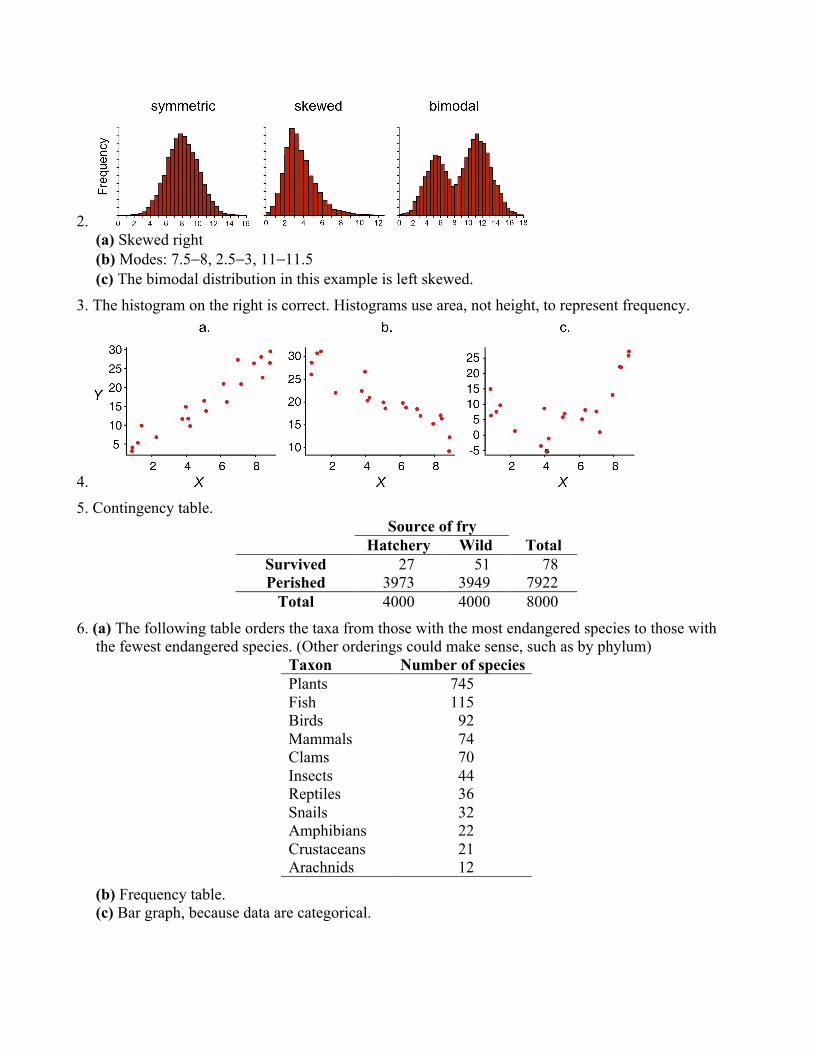
2. (a) Skewed right(b) Modes: 7.5−8, 2.5−3, 11−11.5(c) The bimodal distribution in this example is left skewed.

3. The histogram on the right is correct. Histograms use area, not height, to represent frequency.

4. 5. Contingency table.

Source of fryHatchery Wild Total

Survived 27 51 78Perished 3973 3949 7922

Total 4000 4000 8000

6. (a) The following table orders the taxa from those with the most endangered species to those withthe fewest endangered species. (Other orderings could make sense, such as by phylum)

Taxon Number of speciesPlants 745Fish 115Birds 92Mammals 74Clams 70Insects 44Reptiles 36Snails 32Amphibians 22Crustaceans 21Arachnids 12

(b) Frequency table.(c) Bar graph, because data are categorical.

(d) The baseline should be 0 so that bar height and area correspond to frequency.7. (a) The variables are year (or famine stage) and incidence of schizophrenia. (b) Year (and famine

stage) is categorical – ordinal. Incidence of schizophrenia is categorical – nominal. (c)Contingency table.

1956(pre famine)

1960(famine)

1965(post famine) Total

Schizophrenic 483 192 695 1370Non-schizophrenic 58605 13556 82841 155002

Total 59088 13748 83536 156372

(d) Proportions: 1956: 0.0082, 1960: 0.0140, 1965: 0.0083. Other variations of the line graphbelow are valid (e.g., famine state could be the explanatory variable instead of year)

Pattern revealed: incidence of schizophrenia highest in 1960, the famine year.8. (a) Grouped histograms. (b) Groups are disease types (diseases transmitted directly from one

individual to another and diseases transferred by insect vectors). (c) The variable is the virulenceof the disease. It is a continuous numeric variable. (d) Relative frequency, the fraction ofdiseases occurring in each interval of virulence. (e) Directly transmitted diseases tend to be lessvirulent than insect-transmitted diseases. Human diseases transmitted directly more frequentlyhave low virulence, and less frequently have high virulence, than diseases transmitted by insectvector.

9. (a) Map. (b) Date of first appearance of rabies (measured by the number of months following 1March 1991). (c) Geographic location - the township.

10. (a) Launch temperature is the explanatory variable, number of O-ring failures is the responsevariable. Because we wish to predict failures from temperature.

(b) There is a negative association. (c) Low temperature is predicted to increase the risk of O-ring failure.

11. (a) The distribution is left skewed.(b) The mode is between 65 and 80 degrees (if you used an interval width of 10 degrees instead

of 5 degrees then the mode is between 70 and 80 degrees.12. (a) Husbands of adopted women resemble a woman's adoptive father, more than they resemble

the women themselves or the women’s adoptive mother. (b) Inappropriate baseline. The eye isreceptive to bar height and area, but because of the baseline height and area do not depictmagnitude. A baseline of 0 would probably be best (adding a horizontal line at resemblance = 25might also be a good idea to indicate the random expectation). (c) No, the graph is depicting ameasurement (resemblance) in each of several categories, not frequency of occurrence.

13. (a) Mosaic plot. The explanatory variable is fruit set in previous years. The response variable isfruiting in the given year. Both variables are categorical. (b) Line graph. The explanatoryvariable is year. The response variable is the density of the wood. Both variables are numerical.(c) Grouped cumulative frequency distributions. The explanatory variable is the taxonomic group

(butterflies, birds, or plants). The response variable is the percent change in range size. Groupis a categorical variable. Range change is numerical.

Chapter 31. (a) The number of doctors studied who sterilized a given percentage of patients under age 25.

(b) The median would be more informative. The mean would be sensitive to the presence of theoutlier (sterilizing more than 30% of female patients under 25), whereas the median is notaffected.

2. (a) Box plot. (b) Median body mass of the mammals in each group. (c) The first and thirdquartiles of body mass in each group. (d) “Extreme values”, those lying farther than 1.5 times theinterquartile range from the box edge. (e) Whiskers. They extend to the smallest and largestvalues in the data, excluding extreme values (those lying farther than 1.5 times the interquartilerange from the box edge). (f) Living mammals have the smallest median body size (with a logbody mass of about 2), and mammals that went extinct in the last ice age had the largest mediansize (around 5.5). Mammals that went extinct recently were intermediate in size, with a medianof around 3.2. (g) The body size distribution of living mammals is right skewed (long tail towardlarger values), whereas the size frequency distribution in mammals that went extinct in the lastice age is left skewed. The frequency distribution of sizes is nearly symmetric in mammals thatwent extinct recently. (h) One way to answer this is to use the interquartile range as a measure ofspread, in which case the mammals that went extinct in the last ice age have the lowest spread.Another way to compare spread is to calculate the standard deviation of log body size in eachgroup, but we are unable to calculate this without the raw data. (i) It is likely that extinctionshave reduced the median body size of mammals.

3. (a) Grouped histograms. (b) Explanatory variable: sex. Response variable: Number of words perday. (c) Men: 8,000-12,000 words per day. Women: 16,000-20,000 words per day. (d) Women.(e) Men

4. (a) The averages are 7.5 g for the crimson-rumped waxbill (CW), 15.4 g for the cutthroat finch(CF), and 37.9 g for the white-browed sparrow weaver (WS). (b) Standard deviations are 0.6 gfor CW, 1.2 g for CF, and 3.1 g for WS. The standard deviation is greater when the mean isgreater. (c) Coefficients of variation:8.3% for CW, 8.0% for CF, and 8.2% for WS. Thecoefficients of variation are much more similar than the standard deviations. (d) Comparecoefficients of variation to compare variation relative to the mean. Beak length: 3.8%, Bodymass: 8.2%. Body mass is most variable relative to the mean.

5. Use the cumulative frequency distribution to estimate the median (0.50 quantile, approximately1.4%), the first and third quartiles (approximately 0.7% and 2.4%). The interquartile range isabout 2.4 − 0.7 = 1.6% and 1.5 times this amount is about 2.4%, which sets the maximum lengthof each whisker. The smallest value is about −1.1% and the largest value is about 4.3%. Boththese values are within 1.5 times the interquartile range, so the whiskers extend from −1.1% and4.3%. The boxplot is:

6. (a) cm/s.

(b) (c) Asymmetric. The range of changes in speed is much greater above the median than below themedian. This is true whether we look at the 3rd quartile or the total range. (d) The span of the boxindicates where the middle 50% of the measurements occur (first quartile to third quartile). (e)Mean is 1.19 cm/s, which is greater than the median (0.94). The distribution is right skewed, andthe large values influence the mean more than the median. (f) 1.15 (cm/s)2 (g) The interval fromY − s and Y + s is 0.11 to 2.26. This includes 11 of the 16 observations, or 69%.

7. (a) Increase the mean by k. (b) No effect.

8. (a) Increase Y by 10 times (11.9 mm/s) (b) Increase s by 10 times (10.7 mm/s) (c) Increasemedian by 10 times (9.4 mm /s) (d) Increase interquartile range by 10 times (16.8 mm/s) (e) Noeffect. (f) Increase s2 by 100 times (115.3 (mm/s)2

9. (a) 5.7 hours. (b) 2.4 hours. (c) 83/114 = 0.73 (73%). (d) Median = 5 hours, which is less than themean. The distribution is right skewed, and the large values influence the mean more than themedian.

Chapter 41. (a) 0.22 hours. (b) The sampling distribution of the estimates of the mean time to rigor mortis. (c)

Random sampling from the population of corpses.

2. The median will probably be smaller than the mean. The distribution is right skewed. Extremevalues have a greater effect on the mean, pulling it upwards, than on the median.

3. Sample size.

4. (a) False ( p is just an estimate based on a sample). (b) True (c) True (d) False, this fraction is aconstant. (Leaving aside the possibility of gene copy number variation between people) (e) True

5. (a) The fraction of all Canadians who agree with the statement. (b) The sample estimate is 73%.(c) The sample size is 1641 people. (d) The 95% confidence interval for the population fraction.

6. (a) 95.9 msec. The population mean flash duration. (b) No, because the calculation was based ona sample rather than the whole population. By chance, the sample mean will differ from that ofthe population mean. (c) 1.9 msec. (d) The spread of the sampling distribution of the samplemean. (e) Using the 2SE rule, 95.9+1.9 msec yields 92.2 < µ < 99.7. (f) The interval representsthe most plausible values for the population mean µ. In roughly 95% of random samples fromthe population, when we compute the 95% confidence interval the interval will include the truepopulation mean.

7. The population mean is likely to be small or zero.

Chapter 51. (a) 5/8 (b) 1/4 (c) 7/8 (either in this case means pepperoni or anchovies or both) (d) No. (some

slices have both pepperoni and anchovies) (e) Yes. Olives and mushrooms are mutuallyexclusive (f) No. Pr[mushrooms] = 3/8; Pr[anchovies] = 1/2; if independent, Pr[mushrooms &anchovies] = Pr[mushrooms] × Pr[anchovies] = 3/16. Actual probability = 1/8. Not independent.(g) Pr[anchovies | olives] = 1/2 (two slices have olives: one of these two has anchovies) (h)Pr[olives | anchovies] = 1/4 (four slices have anchovies, one of these has olives) (i) Pr[last slicehas olives] = 1/4 (two slices of the eight have olives; you still get one slice - it doesn't matterwhether your friends pick before you or after you). (j) Pr[two slices with olives] = Pr[first slicehas olives] × Pr[second slice has olives | first slice has olives] = 2/8 × 1/7 = 1/28. (k) Pr[slicewithout pepperoni] = 1 - Pr[slice with pepperoni] = 3/8 (l) Each piece has either one or notopping.

2. Pr[successful hunting) = Pr[find prey] × Pr[captures prey | finds prey] = 0.8 × 0.1 = 0.08.

3. 45 of 273 trees have cavities, so the probability of choosing a tree with a cavity is 45/273 =0.165.

4. (a) Pr[vowel] = Pr[A] + Pr[E] + Pr[I] + Pr[O] + Pr[U] = 8.2% + 12.7% + 7.0% + 7.5% + 2.8% =38.2%. (b) Pr[five randomly chosen letters from an English text would spell "STATS"] = Pr[S]× Pr[T] × Pr[A] × Pr[T] × Pr[S] = 0.063 × 0.091 × 0.082 × 0.091 × 0.063 = 2.7 × 10-6. (Eachdraw is independent, but all must be successful to satisfy the conditions, so we must multiply theprobability of each independent event.) (c) Pr[2 letters from an English text = "e"] = 0.127 ×0.127 = 0.016.

5. (a) Pr[A1 or A4] = Pr[A1] + Pr[A4] = 0.1 + 0.05 = 0.15 (b) Pr[A1 A1) = Pr[A1] × Pr[A1] = 0.1 ×0.1 = 0.01. (This is only true because the individuals mate at random. If we did not know this, wecould not calculate the probability). (c) Pr[not A1 A1] = 1 - Pr[A1 A1] = 1 - 0.01 = 0.99 (d)Pr[two individuals not A1A1] = Pr[not A1 A1] × Pr[not A1 A1] = 0.99 × 0.99 = 0.9801. (e) Pr[atleast one of two individuals chosen at random has genotype A1 A1] = 1 - Pr[neither individual isA1 A1] = 1 - 0.9801 = 0.0199. (f) Pr[three randomly chosen individuals have no A2 or A3 alleles]= Pr[six randomly chosen alleles are not A2 or A3] = Pr[one allele is neither A2 nor A3]6 ;

Pr[one allele is neither A2 nor A3] = 1 - Pr[individual has either A2 or A3] = 1 - [Pr[A2) + Pr[A3)]= 1 - (0.15 + 0.6) = 0.25. Pr[all three lack these alleles] = 0.256 = 0.00024.

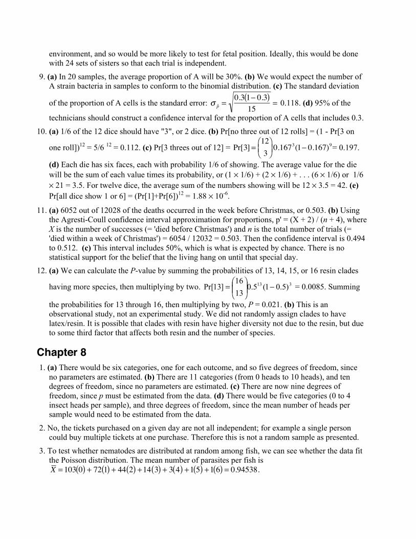
6.

Pr[sum to 7] = 1/6

7. (a) Pr[no venomous snakes] = Pr[not venomous in the left hand] × Pr[not venomous in the righthand]= 3/8 × 2/7 = 6/56 = 0.107(b) Pr[bite]= Pr[bite| 0 venomous snakes] Pr[0 venomous snakes] +

Pr[bite| 1 venomous snakes] Pr[1 venomous snakes] +Pr[bite| 2 venomous snakes] Pr[2 venomous snakes]

Pr[0 venomous snakes] = 0.107 (from part a) Pr[1 venomous snake] = (5/8 × 3/7) + (3/8 × 5/7) = 0.536 Pr[ 2 venomous snakes] = 5/8 × 4/7 = 0.357Pr[bite| 0 venomous snakes] = 0Pr[bite| 1 venomous snake] = 0.8Pr[bite| 2 venomous snakes] = 1 – (1–0.8)2 = 0.96Putting these all together:Pr[bite]= (0 × 0.107) + (0.8 × 0.536) + (0.96 × 0.357) = 0.772

(c)

�

Pr defanged | no bite[ ] =Pr no bite | defanged[ ]Pr defanged[ ]

Pr no bite[ ]Pr[no bite | defanged] = 1; Pr[defanged] = 3/8;Pr[no bite] = Pr[defanged] Pr[no bite |defanged] + Pr[venomous] Pr[no bite | venomous] = (3/8 × 1)+ (5/8 × (1– 0.8)) = 0.5So, [defanged | one snake did not bite] = (1.0 × 3/8) / (0.5) = 0.75.

8. (a) Pr[all five researchers calculate 95% CI with the true value]? Each one has a 95% chance, allsamples are independent, so Pr = 0.955 = 0.774 (b) Pr[at least one does not include trueparameter] = 1 - Pr[all include true parameter] = 1 - 0.774 = 0.226.

9. (a) Pr[cat survives seven days] = Pr[cat not poisoned one day]7 = 0.997 = 0.932 (b) Pr[catsurvives a year] = Pr[cat not poisoned one day]365 = 0.99365 = 0.026 (c) Pr[cat dies within year] =1 - Pr[cat survives year] = 1 - 0.26 = 0.974

10. (a) Pr[single seed lands in suitable habitat] = 0.3 (b) Pr[two independent seeds land in suitablehabitat] = 0.32 = 0.09. (c) Pr[two of three independent seeds land suitable habitat] = 3 × (0.7 ×0.3 × 0.3) = 0.189

11 (a) False positive rate = Pr[positive test | no HIV] = 8 out of 4000 = 0.002 (b) False negative rate= Pr[negative test | HIV] = 20 out of 1000 = 0.02 (c) 988 tested positive, of which 980 had HIV;980/988= 0.9919;

12. Each win has probability 0.09, each loss probability 0.91.(a) Pr[WWLWWW] = 0.095 × 0.91 = 5.4 × 10-6 (b) Pr[WWWWWL] = 0.095 × 0.91 = 5.4 × 10-6

(c) Pr[LWWWWW] = 0.095 × 0.91 = 5.4 × 10-6 (d) Pr[WLWLWL] = 0.093 × 0.913 = 5.5 × 10-4

(e) Pr[WWWLLL] = 0.093 × 0.913 = 5.5 × 10-4 (f) Pr[WWWWWW] = 0.096 = 5.3 × 10-7

13. (a)

The probability that the match lasts two sets is 1/4 + 1/4 = 1/2. The probability that it lasts threegames is 1/8+1/8+1/8+1/8=1/2.

(b)

The probability of the weaker player winning is (0.452 × 0.55) + (0.452 × 0.55) + 0.452 = 0.42525

14. Pr[next person will wash his / her hands] =Pr[wash | man] × Pr[man] + Pr[wash | woman] × Pr[woman] = 0.74 × 0.4 + 0.83 × 0.6 = 0.794

15. Total probability: 4/36 = 1/9 = 0.1116. (a) Pr[one person not blinking] = 1 - Pr[person blinks] = 1 - 0.04 = 0.96 (b) Pr[at least one blink

in 10 people] = 1 - Pr[no one blinks] = 1 - 0.9610 = 0.335

Chapter 61. (a) True. (b) False.

2. (a) H0: The rate of correct guesses is 1/6. (b) HA: The rate of correct guesses is not 1/6. (Wewould argue that a two-tailed test is more appropriate than a one-tailed test⎯ who can say thatESP would work the way we want it to?).

3. (a) Alternative hypothesis. (b) Alternative hypothesis. (c) Null hypothesis. (d) Alternativehypothesis (e) Null hypothesis.

4. (a) Lowers the probability of committing a Type I error. (b) Increases the probability ofcommitting a Type II error. (c) Lowers power of a test. (d) No effect.

5. (a) No effect. (b) Decreases the probability of committing a type II error. (c) Increases the powerof a test. (d) No effect.

6. (a) P = 2 × (Pr[15] + Pr[16] + Pr[17]+Pr[18]) = 0.0075. (b) P = 2 × (Pr[13] + Pr[14] + …. +Pr[18]) = 0.096. (c) P = 2 × (Pr[10] + Pr[11] + Pr[12] + … + Pr[18]) = 0.815. (d) P = 2 × (Pr[1]+ Pr[2] + Pr[3] + … + Pr[7]) = 0.481.

7. False. The hypotheses aren’t variables subject to chance. Rather, the P value measures howunusual the data are if the null hypothesis is true.

8. Failing to reject H0 does not mean H0 is correct, because the power of the test might be limited.The null hypothesis is the default and is either rejected or not rejected.

9. Begin by stating the hypotheses. H0: Size on islands does not differ in a consistent direction fromsize on mainlands in Asian large mammals (i.e., p = 0.5); HA: Size on islands differs in aconsistent direction from size on mainlands in Asian large mammals (i.e., p ≠ 0.5), where p is thetrue fraction of large mammal species that are smaller on islands than on the mainland. Note thatthis is a 2-tailed test. The test statistic is the observed number of mammal species for which sizeis smaller on islands than mainland: 16. The P-value is the probability of a result as unusual as16 our of 18 when H0 is true: P = 2× (Pr[16] + Pr[17] + Pr[18]) = 0.00135. Since P < 0.05, rejectH0. Conclude that size on islands is usually smaller than on mainlands in Asian large mammals.

10. (a) Not correct. The P-value does not give the size of the effect. (b) Correct. H0 was rejected, sowe conclude that there is indeed an effect. (c) Not correct. The probability of committing a TypeI error is set by the significance level, 0.05, which is decided beforehand. (d) Not correct. Theprobability of committing a type II error depended on the effect size, which wasn’t known. (e)Correct.

Chapter 71. (a) 91 / 220 had cancer, so the estimated probability of a cast or crew member developing cancer

is 0.414. (b) The standard error of the proportion is 0.033. [The square-root of (0.414)(1 -0.414)/(220-1). This quantity measures the standard deviation of the sampling distribution of theproportion. (c) Using the Agresti-Coull method to generate confidence intervals, we firstcalculate p' = (x+2)/(n+4) = (91 + 2) / (220 + 4 ) = 0.415.

The lower bound for the 95% confidence interval is 0.415 - 1.96

�

′ p 1− ′ p ( )n + 4

= 0.351

The upper bound is 0.415 + 1.96

�

′ p 1− ′ p ( )n + 4

= 0.480. The confidence intervals do not bracket the

typical 14% cancer rate for the age group. It is unlikely that 14% is the true cancer rate for thisgroup.

2. (a) 46/50 bills had cocaine, so the estimated proportion is 0.92. (b) The 99% confidence interval,calculated using the Agresti-Coull method: p' = 48 / 54 = 0.89. Z for 99% = 2.58. The bounds of

the confidence interval are 0.779 and 0.999. (c) We are 99% confident that the true proportion ofUS one-dollar bills that have a measurable cocaine content lies between 0.779 and 0.999.

3. (a) No; the probability of drawing a red card changes depending on the cards that have beendrawn. (b) Yes: because the sampling is with replacement, the probability of success remainsconstant. (c) No, the probability of drawing a red ball will change with each draw.(d) No, the number of trials is not known. (e) Yes, the number of red-eyed flies in a sample froma large population can be described using the binomial distribution. (Because the populationsampled is large, we will assume that the sampling of each individual has a negligible effect onthe probability of drawing a red fly on the next draw). (f) No, the individuals within differentfamilies may have different probabilities of having red eyes due to shared genetic differences.

4. (a) This estimate pools numbers from two different groups. Women with rosacea are not arandom sample of the population. (b) If the control group women are a random sample, 15/16have mites, 0.938. (c) p'= 17 / 20 = 0.85. The 95% confidence interval is 0.69 to 1.00.(Proportions cannot be larger than 1, so the confidence interval is truncated at 1). (d) For thewomen with rosacea, p' = 18/20 = 0.90. The 95% confidence interval is: 0.769 < p < 1.0.

5. (a) Pr[male is eaten] = 21/52 = 0.404. p'=23/56 = 0.411. The 95% confidence interval is from0.282 to 0.540. (b) This estimate is consistent with a 50% capture of males, but not with a 10%capture of males. (c) The larger sample would not change the estimate of the proportion (thefraction is exactly the same), but it would reduce width of the confidence interval. (The samplesize is in the denominator of the confidence interval equations.)

6. Estimated probability of moving north is 22/24 = 0.917. To test the hypothesis that north andsouth movements of ranges are equally probable, we need to calculate the probability of 22, 23,or 24 species moving northward if p = 0.5. We will make this a two-tailed test, just to satisfy theskeptics, so we'll multiply this probability by two.

222 )5.01(5.02224

]22Pr[ −⎟⎟⎠

⎞⎜⎜⎝

⎛= = 1.6 × 10-5

Doing the same for 23 and 24, summing all three, and multiplying by two, we find that P = 3.6 ×10-5. We can confidently reject the null hypothesis.

7. (a) The first study with the narrower confidence interval probably had the larger sample size. (b)The estimate with the smaller confidence interval is the more believable, in the sense that thetrue value is likely to be somewhere near the estimate. (c) The differences are what we mightexpect due to random sampling: the second confidence interval overlaps the estimate of the firststudy.

8. (a) This is evidence that males' choices may be affected by female positioning of the females: theprobability of seeing 19 of 24 choose the M0 female with null hypothesis that there is nopreference (p = 0.5). With a binomial test,

�

P = 2 Pr 19[ ] + Pr 20[ ] + Pr 21[ ] + Pr 22[ ] + Pr 23[ ] + Pr 24[ ]{ } = 2 0.00253 + 0.0006 + 0.0001 + ...{ } = 0.0066. Therefore P < 0.05, and we can reject the null hypothesis that the males have no preference.(b) However, the males may have preferred one female over the other for a number of reasons. Ifthe females were sisters, this would reduce the number of differences due to genes and maternal

environment, and so would be more likely to test for fetal position. Ideally, this would be donewith 24 sets of sisters so that each trial is independent.

9. (a) In 20 samples, the average proportion of A will be 30%. (b) We would expect the number ofA strain bacteria in samples to conform to the binomial distribution. (c) The standard deviation

of the proportion of A cells is the standard error:

�

σ ˆ p =0.3 1− 0.3( )

15= 0.118. (d) 95% of the

technicians should construct a confidence interval for the proportion of A cells that includes 0.3.

10. (a) 1/6 of the 12 dice should have "3", or 2 dice. (b) Pr[no three out of 12 rolls] = (1 - Pr[3 on

one roll])12 = 5/6 12 = 0.112. (c) Pr[3 threes out of 12] =

�

Pr[3] =123

⎛ ⎝ ⎜

⎞ ⎠ ⎟ 0.1673(1− 0.167)9= 0.197.

(d) Each die has six faces, each with probability 1/6 of showing. The average value for the diewill be the sum of each value times its probability, or (1 × 1/6) + (2 × 1/6) + . . . (6 × 1/6) or 1/6× 21 = 3.5. For twelve dice, the average sum of the numbers showing will be 12 × 3.5 = 42. (e)Pr[all dice show 1 or 6] = (Pr[1]+Pr[6])12 = 1.88 × 10-6.

11. (a) 6052 out of 12028 of the deaths occurred in the week before Christmas, or 0.503. (b) Usingthe Agresti-Coull confidence interval approximation for proportions, p' = (X + 2) / (n + 4), whereX is the number of successes (= 'died before Christmas') and n is the total number of trials (='died within a week of Christmas') = 6054 / 12032 = 0.503. Then the confidence interval is 0.494to 0.512. (c) This interval includes 50%, which is what is expected by chance. There is nostatistical support for the belief that the living hang on until that special day.

12. (a) We can calculate the P-value by summing the probabilities of 13, 14, 15, or 16 resin clades

having more species, then multiplying by two. 313 )5.01(5.01316

]13Pr[ −⎟⎟⎠

⎞⎜⎜⎝

⎛= = 0.0085. Summing

the probabilities for 13 through 16, then multiplying by two, P = 0.021. (b) This is anobservational study, not an experimental study. We did not randomly assign clades to havelatex/resin. It is possible that clades with resin have higher diversity not due to the resin, but dueto some third factor that affects both resin and the number of species.

Chapter 81. (a) There would be six categories, one for each outcome, and so five degrees of freedom, since

no parameters are estimated. (b) There are 11 categories (from 0 heads to 10 heads), and tendegrees of freedom, since no parameters are estimated. (c) There are now nine degrees offreedom, since p must be estimated from the data. (d) There would be five categories (0 to 4insect heads per sample), and three degrees of freedom, since the mean number of heads persample would need to be estimated from the data.

2. No, the tickets purchased on a given day are not all independent; for example a single personcould buy multiple tickets at one purchase. Therefore this is not a random sample as presented.

3. To test whether nematodes are distributed at random among fish, we can see whether the data fitthe Poisson distribution. The mean number of parasites per fish is

�

X = 103 0( ) + 72 1( ) + 44 2( ) +14 3( ) + 3 4( ) +1 5( ) +1 6( ) = 0.94538.

The expected values from a Poisson distribution with this mean are given below, from theproportion expected from the Poisson distribution times the total sample size, n= 238:

Number ofparasites

Observed Expected

0 103 92.471 72 87.422 44 41.323 14 13.024 3 3.085 1 0.586 1 0.09

The expected values for 5 and 6 are below one, so we will combine 4 through 6 into onecategory.

Number ofparasites

Observed Expected

�

Observed − Expected( )2Expected

0 103 92.47 1.201 72 87.42 2.722 44 41.32 0.173 14 13.02 0.07≥4 5 3.75 0.42

χ2 = 4.58. There are five categories, one parameter estimated, so df = 3.

�

χ0.05,32 = 7.81. 4.58 <

7.81, so we cannot reject the random distribution of parasites on fish.4. (a) If pine seedlings are distributed randomly, the frequencies should fit the Poisson distribution.

(b) The mean number of seedlings per quadrat was 1.325.Number ofseedlings

Observed Expected

0 47 21.261 6 28.182 5 18.673 8 8.24≥4 14 3.65

The expected counts for 5-7 were below 1, so 4 through 7 were combined. χ2 = 88.03, with df =3 (five categories, minus one, minus one parameter estimated).

�

χ0.001,32 = 16.27 , and χ2 is greater

than this critical value, so P < 0.001. (c) Seedlings are not distributed at random. (The variance,3.49, is much greater than the mean here, indicating that some quadrats are much more likelythan others to have seedlings: seedlings are clumped.)

5. (a) The mean number of goals per side is 1.26. (b) Fitting this to a Poisson and testing with agoodness of fit test, we must again combine the four goals and above categories to avoidexpected values less than one.

Number ofgoals

Observed Expected

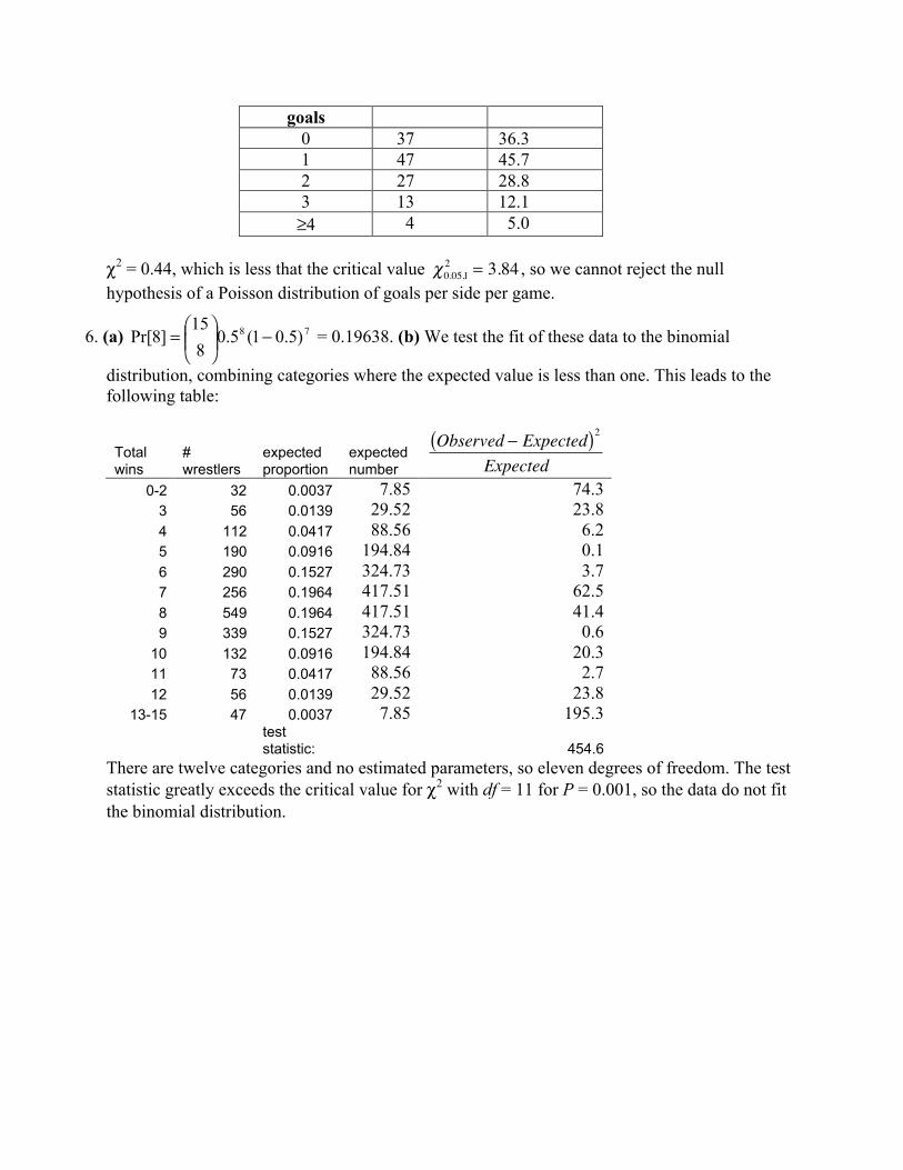
goals0 37 36.31 47 45.72 27 28.83 13 12.1≥4 4 5.0

χ2 = 0.44, which is less that the critical value

�

χ0.05,12 = 3.84 , so we cannot reject the null

hypothesis of a Poisson distribution of goals per side per game.

6. (a) 78 )5.01(5.0815

]8Pr[ −⎟⎟⎠

⎞⎜⎜⎝

⎛= = 0.19638. (b) We test the fit of these data to the binomial

distribution, combining categories where the expected value is less than one. This leads to thefollowing table:

Totalwins

#wrestlers

expectedproportion

expectednumber

�


0-2 32 0.0037 7.85 74.33 56 0.0139 29.52 23.84 112 0.0417 88.56 6.25 190 0.0916 194.84 0.16 290 0.1527 324.73 3.77 256 0.1964 417.51 62.58 549 0.1964 417.51 41.49 339 0.1527 324.73 0.6

10 132 0.0916 194.84 20.311 73 0.0417 88.56 2.712 56 0.0139 29.52 23.8

13-15 47 0.0037 7.85 195.3teststatistic: 454.6

There are twelve categories and no estimated parameters, so eleven degrees of freedom. The teststatistic greatly exceeds the critical value for χ2 with df = 11 for P = 0.001, so the data do not fitthe binomial distribution.

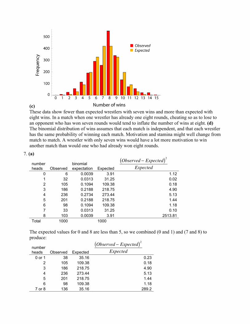
(c)These data show fewer than expected wrestlers with seven wins and more than expected witheight wins. In a match when one wrestler has already one eight rounds, cheating so as to lose toan opponent who has won seven rounds would tend to inflate the number of wins at eight. (d)The binomial distribution of wins assumes that each match is independent, and that each wrestlerhas the same probability of winning each match. Motivation and stamina might well change frommatch to match. A wrestler with only seven wins would have a lot more motivation to winanother match than would one who had already won eight rounds.

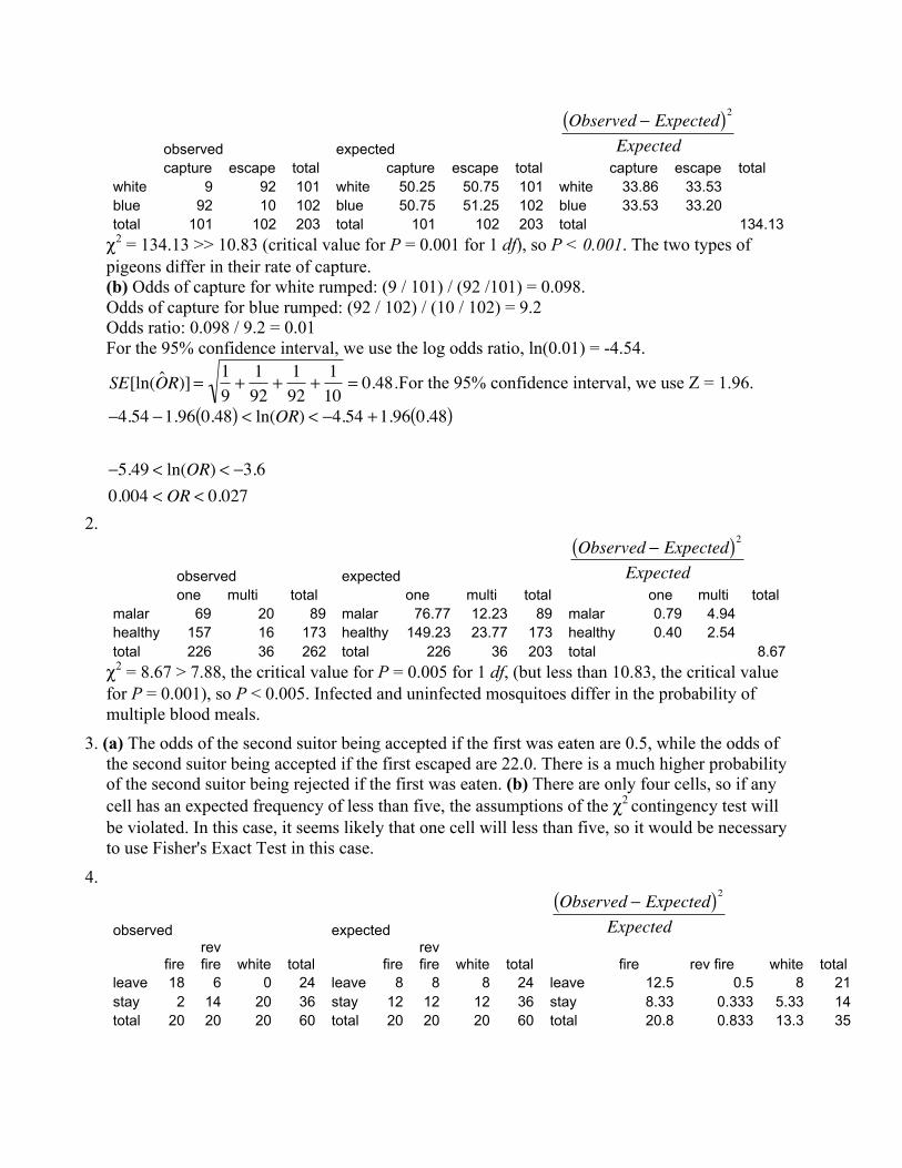
7. (a)

numberheads Observed

binomialexpectation Expected

�


0 6 0.0039 3.91 1.121 32 0.0313 31.25 0.022 105 0.1094 109.38 0.183 186 0.2188 218.75 4.904 236 0.2734 273.44 5.135 201 0.2188 218.75 1.446 98 0.1094 109.38 1.187 33 0.0313 31.25 0.108 103 0.0039 3.91 2513.81

Total 1000 1000

The expected values for 0 and 8 are less than 5, so we combined (0 and 1) and (7 and 8) toproduce:

numberheads Observed Expected

�


0 or 1 38 35.16 0.232 105 109.38 0.183 186 218.75 4.904 236 273.44 5.135 201 218.75 1.446 98 109.38 1.18

7 or 8 136 35.16 289.2

Total 1000 1000 χ2 =302.27

A χ2 goodness-of-fit test to the binomial on these data with the null hypothesis that theproportion of heads is p = 0.5, gives χ2 = 302.3. Reject the null hypothesis with P < 0.001 (df =6). (b) Graphing this, we can see very easily that there is an excess of coins yielding eight heads.(c) We would expect the observed number of coins yielding 8 heads to be roughly equal to thenumber of coins yielding 0 heads, or around 4. This means that there is an excess are two-headedcoins, so roughly 103 – 4 = 99.

8. We will use a goodness of fit test to see whether the data differ from the 0.5 expectation if cancerdeaths were randomly distributed around Christmas.

observed expected

�


die before Xmas 6052 6014 0.24die after Xmas 5976 6014 0.24total deaths 12028

χ2 = 0.48, and df = 1. 0.48 < 3.84, the critical value for P = 0.05, so we do not reject thehypothesis of a random distribution of cancer deaths around Christmas.

9.

observed 14% expected

�


cancer death 91 30.8 117.67non-cancerdeath 129 189.2 19.15total 220 220 test stat: 136.82

df = 1 ; χ2 =136.82 >> 10.83, the critical value for P = 0.001, so we can reject the hypothesis thatthe cast and crew suffered the population-wide cancer mortality rate, P< 0.001.

10. The average admissions are 20 per night. What is the probability of five or fewer admissions?Assume that each admission is independent (no riots, please). Then, they should be Poissondistributed. To find the probability of a quiet night, we sum the probabilities of 0 to 5admissions.

admissions probability0 2.06E-091 4.12E-082 4.12E-073 2.75E-064 1.37E-055 5.50E-05

Total probability = 7.2 × 10-5. Best to keep that coffee brewing: you'll need to work 58 years onaverage before you'll have a quiet night!

Chapter 91. (a)

observed expected

�


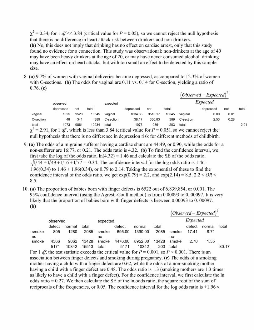
capture escape total capture escape total capture escape totalwhite 9 92 101 white 50.25 50.75 101 white 33.86 33.53blue 92 10 102 blue 50.75 51.25 102 blue 33.53 33.20total 101 102 203 total 101 102 203 total 134.13χ2 = 134.13 >> 10.83 (critical value for P = 0.001 for 1 df), so P < 0.001. The two types ofpigeons differ in their rate of capture.(b) Odds of capture for white rumped: (9 / 101) / (92 /101) = 0.098.Odds of capture for blue rumped: (92 / 102) / (10 / 102) = 9.2Odds ratio: 0.098 / 9.2 = 0.01For the 95% confidence interval, we use the log odds ratio, ln(0.01) = -4.54.

�

SE[ln( ˆ O R)] =19

+1

92+

192

+1

10= 0.48.For the 95% confidence interval, we use Z = 1.96.

�

−4.54 −1.96 0.48( ) < ln(OR) < −4.54 +1.96 0.48( )

−5.49 < ln(OR) < −3.60.004 < OR < 0.027

2.

observed expected

�


one multi total one multi total one multi totalmalar 69 20 89 malar 76.77 12.23 89 malar 0.79 4.94healthy 157 16 173 healthy 149.23 23.77 173 healthy 0.40 2.54total 226 36 262 total 226 36 203 total 8.67χ2 = 8.67 > 7.88, the critical value for P = 0.005 for 1 df, (but less than 10.83, the critical valuefor P = 0.001), so P < 0.005. Infected and uninfected mosquitoes differ in the probability ofmultiple blood meals.

3. (a) The odds of the second suitor being accepted if the first was eaten are 0.5, while the odds ofthe second suitor being accepted if the first escaped are 22.0. There is a much higher probabilityof the second suitor being rejected if the first was eaten. (b) There are only four cells, so if anycell has an expected frequency of less than five, the assumptions of the χ2 contingency test willbe violated. In this case, it seems likely that one cell will less than five, so it would be necessaryto use Fisher's Exact Test in this case.

4.

observed expected

�


firerevfire white total fire

revfire white total fire rev fire white total

leave 18 6 0 24 leave 8 8 8 24 leave 12.5 0.5 8 21stay 2 14 20 36 stay 12 12 12 36 stay 8.33 0.333 5.33 14total 20 20 20 60 total 20 20 20 60 total 20.8 0.833 13.3 35

χ2 = 35.0, for 2 df, (since there are two rows, three columns, so (2-1)(3-1) = 2 df. 35.0>13.82, thecritical value for P = 0.001 for 2 df, so P < 0.001. Yes, there is evidence that reed frogs reactconsistently to the sound of fire.

5.observed expectedjuv m juv f total juv m juv f total

adultm 1 11 12 adult m 3.82 8.18 12adult f 6 4 10 adult f 3.18 6.82 10

7 15 22 total 7 15 22(a) Two of the expected values are less than 5, so we cannot use a χ2 contingency analysis.Fisher's exact test is a good alternative. (b) The effects is in the expected direction.

6. (a) Proportions of kids in each TV viewing class having violent records eight years later, andconfidence intervals (using Agresti-Coull calculations from chapter 7)

record total proportion p' low CI high CI1hr 5 88 0.057 0.0761 0.022 0.1301-3hr 87 386 0.225 0.2282 0.187 0.2703+hr 67 233 0.288 0.2911 0.233 0.349

(b) Contingency table for test of independence of TV watching and later violent record.

observed expected

�


classnorecord record total class

norecord record total class

norecord record total

1hr 83 5 88 1hr 68.21 19.79 88 1hr 3.21 11.051-3hr 299 87 386 1-3 hr 299.2 86.81 386 1-3 hr 0.0001 0.00043+ hr 166 67 233 3+ hr 180.6 52.4 233 3+ hr 1.18 4.068

548 159 707 548 159 707 19.5χ2 = 19.5, for 2 df, (since there are three rows, two columns, so (3-1)(2-1) = 2 df. 35.0>13.82, thecritical value for P = 0.001 for 2 df, so P < 0.001. There is a relationship between watching TVand future violence: those that watched less than one hour TV were less likely to have a record,while those that watched three or more hours were more likely to have a record.(c) No, this does not prove that TV watching causes aggression in kids. This was anobservational study, not experimental, so we do not know if kids watching more TV have otherfactors in common (e.g. lower parental supervision, etc.).

7.

observed expected

�


arrest healthy total arrest healthy total arrest healthy totalabstainers 12 197 209 abstainers 10.70 198.30 209 abstainers 0.16 0.01drinkers 9 192 201 drinkers 10.30 190.70 201 drinkers 0.16 0.01total 21 389 410 total 21 389 203 total 0.34

χ2 = 0.34, for 1 df << 3.84 (critical value for P = 0.05), so we cannot reject the null hypothesisthat there is no difference in heart attack risk between drinkers and non-drinkers.(b) No, this does not imply that drinking has no effect on cardiac arrest, only that this studyfound no evidence for a connection. This study was observational: non-drinkers at the age of 40may have been heavy drinkers at the age of 20, or may have never consumed alcohol. drinkingmay have an effect on heart attacks, but with too small an effect to be detected by this samplesize.

8. (a) 9.7% of women with vaginal deliveries became depressed, as compared to 12.3% of womenwith C-sections. (b) The odds for vaginal are 0.11 vs. 0.14 for C-section, yielding a ratio of0.76. (c)

observed expected

�


depressed not total depressed not total depressed not totalvaginal 1025 9520 10545 vaginal 1034.83 9510.17 10545 vaginal 0.09 0.01C-section 48 341 389 C-section 38.17 350.83 389 C-section 2.53 0.28total 1073 9861 10934 total 1073 9861 203 total 2.91

χ2 = 2.91, for 1 df , which is less than 3.84 (critical value for P = 0.05), so we cannot reject thenull hypothesis that there is no difference in depression risk for different methods of childbirth.

9. (a) The odds of a migraine sufferer having a cardiac shunt are 44:49, or 0.90, while the odds for anon-sufferer are 16:77, or 0.21. The odds ratio is 4.32. (b) To find the confidence interval, wefirst take the log of the odds ratio, ln(4.32) = 1.46 and calculate the SE of the odds ratio,

�

1 44 +1 49 +1 16 +1 77 = 0.34. The confidence interval for the log odds ratio is 1.46 -1.96(0.34) to 1.46 + 1.96(0.34), or 0.79 to 2.14. Taking the exponential of these to find theconfidence interval of the odds ratio, we get exp(0.79) = 2.2, and exp(2.14) = 8.5. 2.2 < OR <8.5.

10. (a) The proportion of babies born with finger defects is 6522 out of 6,839,854, or 0.001. The95% confidence interval (using the Agresti-Coull method) is from 0.00093 to 0. 00097. It is verylikely that the proportion of babies born with finger defects is between 0.00093 to 0. 00097.(b)

observed expected

�


defect normal total defect normal total defect normal totalsmoke 805 1280 2085 smoke 695.00 1390.00 2085 smoke 17.41 8.71nosmoke 4366 9062 13428

nosmoke 4476.00 8952.00 13428

nosmoke 2.70 1.35

5171 10342 15513 total 5171 10342 203 total 30.17For 1 df, the test statistic exceeds the critical value for P = 0.001, so P < 0.001. There is anassociation between finger defects and smoking during pregnancy. (c) The odds of a smokingmother having a child with a finger defect are 0.62, while the odds of a non-smoking motherhaving a child with a finger defect are 0.48. The odds ratio is 1.3 (smoking mothers are 1.3 timesas likely to have a child with a finger defect). For the confidence interval, we first calculate the lnodds ratio = 0.27. We then calculate the SE of the ln odds ratio, the square root of the sum ofreciprocals of the frequencies, or 0.05. The confidence interval for the log odds ratio is +1.96 ×

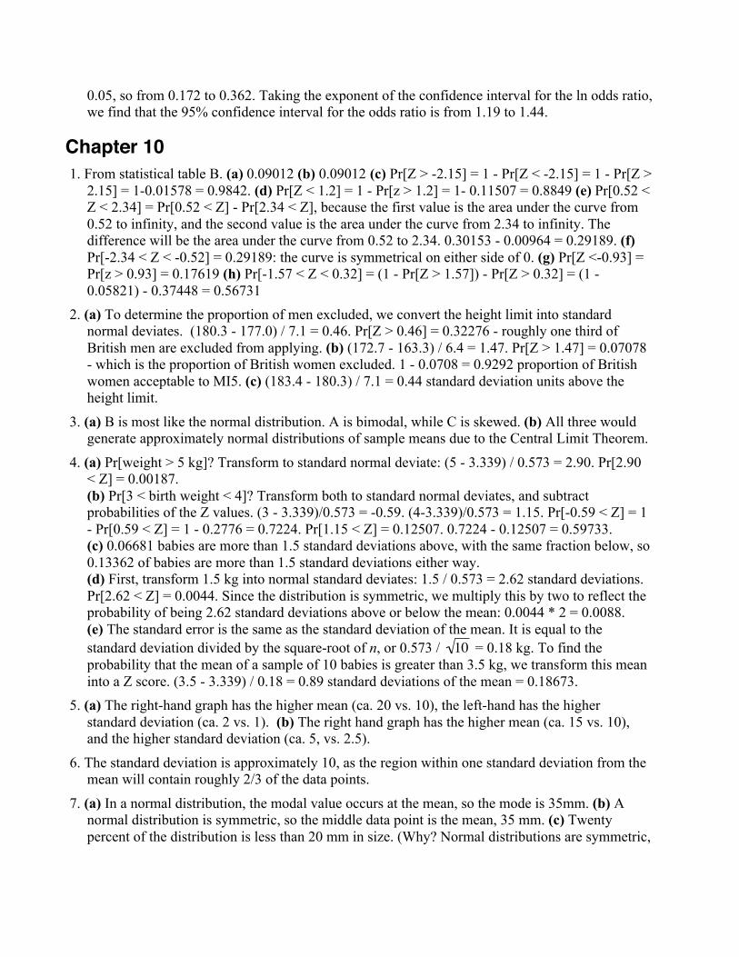
0.05, so from 0.172 to 0.362. Taking the exponent of the confidence interval for the ln odds ratio,we find that the 95% confidence interval for the odds ratio is from 1.19 to 1.44.

Chapter 101. From statistical table B. (a) 0.09012 (b) 0.09012 (c) Pr[Z > -2.15] = 1 - Pr[Z < -2.15] = 1 - Pr[Z >

2.15] = 1-0.01578 = 0.9842. (d) Pr[Z < 1.2] = 1 - Pr[z > 1.2] = 1- 0.11507 = 0.8849 (e) Pr[0.52 <Z < 2.34] = Pr[0.52 < Z] - Pr[2.34 < Z], because the first value is the area under the curve from0.52 to infinity, and the second value is the area under the curve from 2.34 to infinity. Thedifference will be the area under the curve from 0.52 to 2.34. 0.30153 - 0.00964 = 0.29189. (f)Pr[-2.34 < Z < -0.52] = 0.29189: the curve is symmetrical on either side of 0. (g) Pr[Z <-0.93] =Pr[z > 0.93] = 0.17619 (h) Pr[-1.57 < Z < 0.32] = (1 - Pr[Z > 1.57]) - Pr[Z > 0.32] = (1 -0.05821) - 0.37448 = 0.56731

2. (a) To determine the proportion of men excluded, we convert the height limit into standardnormal deviates. (180.3 - 177.0) / 7.1 = 0.46. Pr[Z > 0.46] = 0.32276 - roughly one third ofBritish men are excluded from applying. (b) (172.7 - 163.3) / 6.4 = 1.47. Pr[Z > 1.47] = 0.07078- which is the proportion of British women excluded. 1 - 0.0708 = 0.9292 proportion of Britishwomen acceptable to MI5. (c) (183.4 - 180.3) / 7.1 = 0.44 standard deviation units above theheight limit.

3. (a) B is most like the normal distribution. A is bimodal, while C is skewed. (b) All three wouldgenerate approximately normal distributions of sample means due to the Central Limit Theorem.

4. (a) Pr[weight > 5 kg]? Transform to standard normal deviate: (5 - 3.339) / 0.573 = 2.90. Pr[2.90< Z] = 0.00187.(b) Pr[3 < birth weight < 4]? Transform both to standard normal deviates, and subtractprobabilities of the Z values. (3 - 3.339)/0.573 = -0.59. (4-3.339)/0.573 = 1.15. Pr[-0.59 < Z] = 1- Pr[0.59 < Z] = 1 - 0.2776 = 0.7224. Pr[1.15 < Z] = 0.12507. 0.7224 - 0.12507 = 0.59733.(c) 0.06681 babies are more than 1.5 standard deviations above, with the same fraction below, so0.13362 of babies are more than 1.5 standard deviations either way.(d) First, transform 1.5 kg into normal standard deviates: 1.5 / 0.573 = 2.62 standard deviations.Pr[2.62 < Z] = 0.0044. Since the distribution is symmetric, we multiply this by two to reflect theprobability of being 2.62 standard deviations above or below the mean: 0.0044 * 2 = 0.0088.(e) The standard error is the same as the standard deviation of the mean. It is equal to thestandard deviation divided by the square-root of n, or 0.573 /

�

10 = 0.18 kg. To find theprobability that the mean of a sample of 10 babies is greater than 3.5 kg, we transform this meaninto a Z score. (3.5 - 3.339) / 0.18 = 0.89 standard deviations of the mean = 0.18673.

5. (a) The right-hand graph has the higher mean (ca. 20 vs. 10), the left-hand has the higherstandard deviation (ca. 2 vs. 1). (b) The right hand graph has the higher mean (ca. 15 vs. 10),and the higher standard deviation (ca. 5, vs. 2.5).

6. The standard deviation is approximately 10, as the region within one standard deviation from themean will contain roughly 2/3 of the data points.

7. (a) In a normal distribution, the modal value occurs at the mean, so the mode is 35mm. (b) Anormal distribution is symmetric, so the middle data point is the mean, 35 mm. (c) Twentypercent of the distribution is less than 20 mm in size. (Why? Normal distributions are symmetric,

so if 20% of the distribution is 15 mm or larger than the mean, 20% must be 15 mm or smallerthan the mean.)

8. (a) The right-hand distribution (II.) would more have sample means that had a more normaldistribution, because the initial distribution is closer to normal. Both distributions wouldconverge to a normal distribution if the sample size were sufficiently large. (b) The distributionof the sums of samples from a distribution will be normally distributed, given a sufficiently largenumber of samples.

9. (a) The probability of sampling haplotype A is p = 0.3. We expect a sample of 400 fish to have0.3 × 400 A individuals on average, or 120. The standard deviation is approximately

�

n p 1− p( ) = 400 0.3( ) 0.7( ) = 9.17. To find the probability of sampling 130 or more ofhaplotype A, we convert this into a standard normal deviate: (130 - 120) / 9.17 = 1.09; Pr[1.09 <Z] = 0.13786. (b) Pr[at least 300 B haplotype out of 400]? Average number of B sampled = (1-p)× 400 = 280. Convert to standard normal: (300 - 280) / 9.17 = 2.18; Pr[2.18 < Z] = 0.01463. (c)Pr[115 < freq A < 125]? Convert to standard normal deviates, find the probabilities, andcalculate the difference. (115-120)/9.17 = -0.55. (125 - 120)/ 9.17 = 0.55. Pr[-0.55 < Z] = 1 -Pr[0.55 < Z] = 1 - 0.29116 = 0.70884. Pr[0.55 < Z] = 0.29116. 0.70884 - 0.29116 = 0.41768.

10. Average expected number of cancer victims = 0.14 × 220 = 30.8. Standard deviation =

�

n p 1− p( ) = 220 0.14( ) 0.86( ) = 5.15 . Convert actual number of victims, 91, into standardnormal deviate: (91 - 30.8) / 5.15 = 11.7. This is off the chart: P < 0.00002.

11. SE =

�

s n . Z = (y - mean) / SE.Mean SD y SE 10 Z10 Pr(Y > y) SE30 Z30 Pr(Y > y)

14 5 15 1.58 0.63 0.26435 0.91 1.10 0.1356715 3 15.5 0.95 0.53 0.29806 0.54 0.91 0.18141-23 4 -22 1.26 0.79 0.21476 0.73 1.37 0.0853472 50 45 15.81 -1.71 0.95637 9.18 -2.96 0.99846

Chapter 111. The 99% confidence interval must be larger than the 95% confidence interval, in order to have a

higher probability of capturing the true mean.2. (a) The sample mean is 10.32 cm and the standard error of the mean is 0.056 cm. If we sampled

this wolf population repeatedly, 68% of the estimates of the mean would lie between 10.32 ±0.056. (b) The 95% confidence interval for the mean is 10.32 ± (0.056 t0.05(2),34 ). t = 2.03, so the95% confidence interval is: 10.21 < µ < 10.44 cm. (c) The variance is 0.11005. There are 35individuals, so 34 df. The χ2 critical values are looked up in Statistical Table A for α = 0.01 / 2and α = 1 - (0.01 / 2) are 58.96 and 16.50. We now calculate the lower bound of the confidenceinterval: 34 (0.11005) / 58.96 = 0.063. The upper bound is 34 (0.11005) / 16.5 = 0.227. 0.063 <σ 2< 0.227. (d) The 99% confidence interval of the standard deviation of the sample is found bytaking the square-root of the variance confidence interval: 0.252 < σ < 0.476, around theestimated standard deviation of 0.332.

3. No, using n = 70 would assume that the right distance was independent of the left distance. Thisisn't likely, as most animals are symmetric, so we would expect similar distances on each side ofthe mouth.

4. (a) To test whether the mean fitness changed, we will test whether the mean fitness after 100generations was significantly different from 0. For this, we will use a t-test. We need the samplemean, the sample standard error, and the sample size. Our hypothesized value from the nullhypothesis of no change in fitness, µ0, is 0. The mean is 0.2724, the standard deviation is 0.600,and the sample size is 5. From this, we calculate the SE = s /

�

n = 0.6 /

�

5 = 0.268, and wecalculate the t-statistic: t = (mean - µ0 ) / SE = (0.2724 - 0) / 0.268 = 1.02. This is a two-tailedtest, so we look up the critical value of α(2) = 0.05 for 4 df, 2.78. t < tcrit = 2.78, so we do notreject the null hypothesis of no change in fitness. (b) The 95% confidence interval for the meanfitness change is 0.2724+2.78(0.268) : -0.47 < µ < 1.02. (c) We are assuming that fitness isnormally distributed and that the five lineages are random and independent.

5. (a) The mean testes area for monogamous lines is 0.848, while the mean area for polyandrouslines is 0.950. The standard deviation was 0.031 and 0.034 for the two sets. (b) The standarderror of the mean is 0.015 for the monogamous lines and 0.017 for the polyandrous lines. (c) The95% confidence interval for the mean in the polyandrous line is 0.95 ± 0.017t0.05(2),3 =0.95 ± 3.18 (0.017), or 0.90 < µ < 1.00. (d) The 99% CI for the standard deviation of testes areaamong monogamous lines requires the sample variance (0.001), the degrees of freedom (3), andthe critical values of the χ2 distribution for the appropriate α and df. The χ2 critical values arelooked up in Statistical Table A for α =0.01 / 2 and 1 - (0.01 / 2) are 0.07 and 12.84. Then, the99% CI for the variance is 3 (0.001) / 0.07 and 3 (0.001) / 12.84, or 0.0002 to 0.04. To get the99% CI for the standard deviation, we take the square root of each of these, or 0.015 < σ < 0.20.

6. (a) The 95% CI for the discontinuity score requires the estimated mean (0.183), the SE(calculated as the s divided by

�

n , or 0.051), and the critical t value for α(2) = 0.05 for 6 df,2.45. Then the CI is 0.18 ± (0.051 * 2.45) , or 0.058 < µ < 0.308. (b) To test whether the samplemean continuity score of 0.183 is consistent with the predicted mean, µ0 = 0, we use the t-test. t= (mean - µ0) / SE = (0.183 - 0) / 0.051 = 3.6. The critical value for α(2) = 0.05 for 6 df is 2.45. t> tcrit, so we reject the null hypothesis that the mean discontinuity score is zero.

7. In this case, we want to see if rats do better than the chance performance, so we are comparingtheir scores with µ0 = 0.5. The mean is 0.684, the standard deviation is 0.071. There were sevenrats, so SE = 0.071 /

�

7= 0.027. t = (0.684 - 0.5) / 0.027 = 6.82. For α(2) = 0.05, tcrit for six df =2.45; t > tcrit so we reject the null hypothesis that rats were doing as expected by chance.(Moreover, we can show that P < 0. 002.) (For this we assumed that the seven rats were random,independent samples and that their performance scores were normally distributed).

8. Mean coconut weight is 3.2 kg, upper 95% CI bound is 3.5 kg. The confidence interval for themean is symmetric, so the lower bound must be 0.3 kg below the mean, or at 2.9 kg.

9. The confidence interval of the variance is the square of the bounds for the standard deviation.

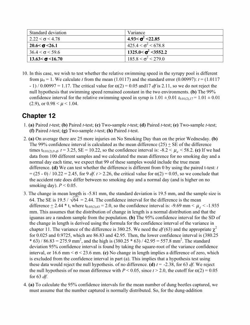
Standard deviation Variance2.22 < σ < 4.78 4.93< σ2 <22.8520.6< σ <26.1 425.4 < σ2 < 678.836.4 < σ < 59.6 1325.0< σ2 <3552.213.63< σ <16.70 185.8 < σ2 < 279.0

10. In this case, we wish to test whether the relative swimming speed in the syrupy pool is differentfrom µ0 = 1. We calculate t from the mean (1.0117) and the standard error (0.00997): t = (1.0117- 1) / 0.00997 = 1.17. The critical value for α(2) = 0.05 and17 df is 2.11, so we do not reject thenull hypothesis that swimming speed remained constant in the two environments. (b) The 99%confidence interval for the relative swimming speed in syrup is 1.01 ± 0.01 t0.01(2),17 = 1.01 ± 0.01(2.9), or 0.98 < µ < 1.04.

Chapter 121. (a) Paired t-test; (b) Paired t-test; (c) Two-sample t-test; (d) Paired t-test; (e) Two-sample t-test;

(f) Paired t-test; (g) Two-sample t-test; (h) Paired t-test.2. (a) On average there are 25 more injuries on No Smoking Day than on the prior Wednesday. (b)

The 99% confidence interval is calculated as the mean difference (25) + SE of the differencetimes t0.01(2),9 df. t = 3.25, SE = 10.22, so the confidence interval is: -8.2 <

�

µd < 58.2. (c) If we haddata from 100 different samples and we calculated the mean difference for no smoking day and anormal day each time, we expect that 99 of these samples would include the true meandifference. (d) We can test whether the difference is different from 0 by using the paired t-test: t= (25 - 0) / 10.22 = 2.45, for 9 df. t > 2.26, the critical value for α(2) = 0.05, so we conclude thatthe accident rate does differ between no smoking day and a normal day (and is higher on nosmoking day). P < 0.05.

3. The change in mean length is -5.81 mm, the standard deviation is 19.5 mm, and the sample size is64. The SE is 19.5 /

�

64 = 2.44. The confidence interval for the difference is the meandifference + 2.44 * t, where t0.05(2),63 = 2.0, so the confidence interval is: -9.69 mm <

�

µd < -1.935mm. This assumes that the distribution of change in length is a normal distribution and that theiguanas are a random sample from the population. (b) The 95% confidence interval for the SD ofthe change in length is derived using the formula for the confidence interval of the variance inchapter 11. The variance of the difference is 380.25. We need the df (63) and the appropriate χ2

for 0.025 and 0.9725, which are 86.83 and 42.95. Then, the lower confidence interval is (380.25* 63) / 86.83 = 275.9 mm2, and the high is (380.25 * 63) / 42.95 = 557.8 mm2. The standarddeviation 95% confidence interval is found by taking the square-root of the variance confidenceinterval, or 16.6 mm < σ < 23.6 mm. (c) No change in length implies a difference of zero, whichis excluded from the confidence interval in part (a). This implies that a hypothesis test usingthese data would reject the null hypothesis. of no difference. (d) t = -2.38, for 63 df. We rejectthe null hypothesis of no mean difference with P < 0.05, since t > 2.0, the cutoff for α(2) = 0.05for 63 df.

4. (a) To calculate the 95% confidence intervals for the mean number of dung beetles captured, wemust assume that the number captured is normally distributed. So, for the dung-addition

treatment, the confidence interval is 4.8 + (2.26 × 1.03): 2.47 < µ < 7.13. For the control, theconfidence interval is 0.51 + (2.26 × 0.28), or -0.13 < µ < 1.15. (b) The two-sample t-test cannotbe used test for differences in the means, since the standard deviations are more than three-folddifferent between the two groups. Instead, a Welch's approximate t-test is appropriate.

5. Because these are not paired samples, we will analyze the difference of the means, not the meanof the differences. The monogamous flies had a mean testes size of 0.8475 mm2, the polyandrous0.95 mm2, for a difference of 0.1025 mm2. The 95% confidence interval for this differencerequires finding the SEY1bar - Y2bar ,= √(sp

2(1/n1 + 1/n2), where n1 and n2 = 4, and sp2 = (df1s1

2 +df2s2

2 )/ (df1 + df2), where df1 = df2 = 3, and s12 and s2

2 = 0.0010 and 0.0011 respectively. Then,SEY1bar - Y2bar = 0.023. The confidence interval for the difference is the standard error timest0.05(2),6 = 2.45, so 0.1025+ 2.45 × 0.23, or 0.046 to 0.159. (b) The null hypothesis is that there isno difference between the monogamous and polyandrous treatments in testes size, so (µ1 - µ2)0 =0. t = the difference in means, 0.1025, over the SE of the difference, 0.23. t = 4.48, for 6 df. tcrit =3.71 for P = 0.01, so P < 0.01. The mean testes sizes are significantly different.

6. (a) On average, 33% more of the male bodies were covered if they emitted pheromones. sp =26.5%;

�

SE Y 1 −Y 2= 6.02%. df1 = 48 and df2 = 31, so df = 79. t0.05(2), 79 df = 1.99, so the confidence

interval is: 21% <

�

µ1 − µ2 < 45%. (b) Using a two-sample t-test, we will assume that the percentcoverage is normally distributed, that each snake is independent, and that the standard deviationsare not different (they are not more than threefold different). The null hypothesis is that there isno difference between the males emitting pheromones and those not, so (µ1 - µ2)0 = 0. t = 0.33 /0.0602 = 5.47 > 3.9, the critical value for α(2) = 0.0002 for 79 df, so we can reject the nullhypothesis, with P < 0.0002.

7. (a) The PLFA levels between the control and addition plots before cicada death were notsignificantly different (two sample t-test: t = -0.19, df = 42, P > 0.10). (b) After the cicadaaddition, the PLFA levels differed significantly: t = 2.89, df = 42, P < 0.01. (c) No: we areinterested in the effect of the cicada addition, so we need to look at whether the change in PLFAlevels differed between the treatments. The correct comparison is the mean change in the controlplots compared to the mean change in the addition plots. It is possible to have a situation inwhich test b was significant and test a was not, but the effect of cicada addition was notsignificant. For instance, the control plots may have been non-significantly lower in PLFA priorto cicada addition, and significantly lower after cicada addition, but the difference might not besignificant.

8. As described, this test assumes that the eight "open water" samples were independent of the eight"near shore" samples, as it uses a two-sample t-test (and so would have 14 df). Differences ingrowth rate could be due to differences between lakes, so the two samples within each lake arenot independent. The paired t-test would better reflect this (and would have 7 df).

9. (a) Since we assume that the distributions are normal, we can use the F-test to compare thevariances. The ratio of the variances (the larger variance is always in the numerator) is F =(0.1582)2/(0.0642)2 = 0.025 / 0.004 = 6.07. The degrees of freedom are 32 and 19. F0.05(1),32,19 =2.05 (between 2.07 for 30 df in the numerator and 2.03 for 40 df), so we reject the nullhypotheses that the variances are equal. (b) The variances are not equal, but the difference in thestandard deviations is not greater than threefold. Therefore a two-sample t-test could be used: t =

0.28, df= 51, P > 0.05. You could use Welch's approximate t test rather than the two-sample t-test. t = 0.13, with 46 df, which is not significant.

10. (a) Remember to multiply each value of flower length by the number of flowers in that category,when calculating the mean and variance (the zeros are dropped in the equation below):

�

4 55( ) +10 58( ) + 41 61( ) + 75 64( ) + 40 67( ) + 3 70( )4 +10 + 41+ 75 + 40 + 3

= 63.5

�

4 55 − 63.5( )2 +10 58 − 63.5( )2 + 41 61− 63.5( )2 + 75 64 − 63.5( )2 + 40 67 − 63.5( )2 + 3 70 − 63.5( )2(4 +10 + 41+ 75 + 40 + 3) −1

= 8.6

(b) For the simplest test, we will assume that distributions are normal. Then we can use the F-test to compare the variances. 42.4 / 8.6 = 4.93; 443, 172 df. Looking this up (roughly) we findthat the critical value is 1.21 (for 1000,200) and 1.31 (for 200,100) for α(1) = 0.05, so weconclude that the variance for the F2 is significantly greater than the variance for the F1.

11. Paired t-test: mean difference is 22.3, which is significantly different from 0 (P <0.01, t = 4.5,df=7).

12. (a) We would use Welch's approximate t-test for this comparison since the standard deviationsdiffer between Pteronotus and the vampires, by more than threefold. (b) The average strengthwas higher for Pteronotus, which is in the opposite direction as predicted by the model.

13. (a) We can use a paired t-test in this case, as the body temperature measurements are taken onthe same individuals as the brain temperature measurements. To do this, we calculate thedifference in temperature between brains and bodies for each ostrich, find the mean difference(0.648 degrees C) and the standard error of the difference (0.116 degrees C). µ0 = 0: the nullhypothesis is that the brain temperature does not differ from the body temperature. t = 0.648 /0.116 = 5.6, with 5 df, which is greater than the critical value for α(2) = 0.01, 4.03, so P < 0.01.We reject the null hypothesis of no difference between brain and body temperature. (b) Whileour test is significant, the deviation is the opposite predicted from observations of mammals insimilar environments: brains are hotter than bodies in ostriches, not cooler.

14. (a) B. (b) B. (c) From B, we can still be fairly confident that the groups are different, but weneed to mentally double the size of the error bars to make this determination. (d) With samplesizes of 100, the standard errors will be one tenth as great as the standard deviations. Graphs A,B, and C will be significantly different.

Chapter 131. (A) The point fall on a curve, not a line, so the distribution is unlikely to be normal. (B) There is

some curvature to this distribution, more than would be expected for a normal distribution. (C)This is very close to the straight line distribution with the points more densely clustered at thecenter that you would expect from a normal distribution. (D) This quantile plot has two distinctcurves. The middle of the plot has relatively few points, not the highest density that you wouldexpect with a normal distribution.

2. (a) I. No, this is a uniform distribution, not a normal distribution.II. No, this plot is bimodal, not normal.

III. No, this plot is right skewed. It looks log-normal rather than normal.IV. Yes, this is a normal distribution.(b) I. The sign test would be best for these data, as they are unlikely to transformed into anythingresembling normal.II. The sign test would probably be best for this distribution as well. Bimodal distributions aretough to transform into anything else.III. These data could probably be tested by a one-sample t-test after transformation (probably alog transformation, as it is right-skewed).IV. These data could be tested by a one-sample t-test as they are.(c) I: B (this explains why there is such a constant density of points in the quantile plots).II: D. (The two peaks correspond to the two curves in the quantile plots; these are also the areasof the highest density in the quantile plots).III. A. (The density is highest on the left, with a few points on the right scattered over a largerange on the x-axis).IV. C. (Sparse points at the extremes of the range; points falling along a straight line as expectedfor a normal distribution).

3. (a) mean 2.75; 95% CI: -3.28 < µlog[x] < 8.78. (b) mean 1.86; 95% CI: -0.02 < µlog[x] < 3.74. (c)Not possible: cannot use ln transformation on negative values. (d) mean 4.23; 95% CI: -2.04 <µlog[x] < 10.5. (e) Here, we must use Y' = ln(Y + 1). Mean: 0.98; 95% CI: -0.23 < µlog[x] < 2.2.

4. After applying the arcsine to the square-root of the raw data, the mean is 1.39 and the SD is 0.09.5. The simplest analysis is a sign test. We will score each lobster as "+" if it is pointing more

towards home than away (so -90 to 90) and "-" if pointing more away than towards home (morethan 90 or less than -90). Lobsters exactly at 90 or -90 will not be scored. Of the 14 scored

lobsters, 11 were "+" and 3 were "-".

�

P = 214x

⎛ ⎝ ⎜

⎞ ⎠ ⎟ 0.514−x0.5x

x=11

14

∑⎛ ⎝ ⎜

⎞ ⎠ ⎟ = 0.057 . Using the usual

standard of α = 0.05, we cannot reject the null hypothesis with these data.

6. Mann-Whitney U test : U1 = 39. U2 =6, so U = 39. The critical value for n1 = 5 and n2 = 9 is 38.U is larger, so we reject the null hypothesis that there is no difference in the time untilreproduction due to accidental death or infanticide.

7. A non-parametric approach to this problem is the Mann-Whitney U test, noting that there will bemany ties, so our test will be less powerful than it might be. We assign a rank of "3" to the zeros(the average of 1-5), a rank of 11.5 to the 1's (average of 6-17), a rank of 19.5 to the 2's (averageof 18-21), and a rank of 23 to the 3's (average of 22-24). Then we sum the ranks for the blindgroup: R1 = 140.5. We then calculated U1 = n1n2 + n1(n1+1)/2 - R1 = 81.5. U2 = n1n2 - U1 = 144 -81.5 = 62.5. U = 81.5. The critical value for n1 = 12 and n2 = 12 is 107. U is smaller, so we donot reject the null hypothesis that there is no difference in the number of gestures used by theblind vs. sighted humans.

8. (a) Benton: mean 0.67, variance 0.075; Warrenton: mean: 0.24, variance 0.007. The standarddeviations are more than 3 fold different, so a two-sample t-test is inappropriate. (b) (1) Try a logtransformation, followed by a two-sample t-test. (2) Welch's t-test on the non-transformed data,which does not require equal variances. (3) Mann-Whitney U test. (c) A log transformationmight be appropriate because the population with the larger mean has the larger variance. Thetwo-sample t-test on the transformed data rejects the null hypothesis: t = 0.961 / 0.249 = 3.87,

with 10 df. P < 0.01. (d) For Benton county, -0.94 < µlog[x] < -0.04. For Warrenton county, -1.84< µlog[x] < -1.06. (e) The transformed confidence interval for Benton county is 0.39 to 0.96; forWarrenton county the interval is 0.16 to 0.35. If we found the means from many samples, 95% ofthe confidence intervals from these samples would contain the true mean.

9. Two-sample t-tests and confidence intervals are robust to violations of equal standard deviationsso long as the sample sizes of the two groups are roughly equal and the standard deviations arewithin 3 times of one another.

10. (A) two-sample t-test (B) These distributions are skewed right, so a log-transformation could betried. (C) This one is tough: neither distribution is normal, but they deviate in different ways, sothat a transformation that would improve the fit for one would not help with the other. Also, thestandard deviations will be very different. The differences in shape make the rank-sum testinappropriate. A randomization test (chapter 19) is best. (D) two-sample t-test. (E) two-sample t-test.

11. (a) The null hypothesis was that the spermatids of males and hermaphrodites did not differ intheir mean size, while the alternative hypothesis is that they do differ in size. (b) U = 35910, n1

= 211, n2 = 700. Use the normal approximation:

�

Z = 2U − n1n2n1n2 n1 + n2 +1( ) /3

= -11.32. This is highly

significant (P < 0.00002). (c) It is not clear whether the variables are distributed in the sameway for the hermaphrodites and the males: if not, the Mann-Whitney U test may be inaccurate.

12. Mann-Whitney U tests are insensitive to outliers and may be used appropriately in this case.

13. The differences are not normally distributed, but skewed right. We need a sign test. There are 6"-" and 22 "+", where a "+" means more species in the dioecious group.

�

P = 228x

⎛ ⎝ ⎜

⎞ ⎠ ⎟ 0.528−x0.5x

x=22

28

∑⎛ ⎝ ⎜

⎞ ⎠ ⎟ = 0.0037, so we reject the null hypothesis.

14. First, we transform the data by taking the natural log of each weight. The mean ln-transformedweights are -1.37 mg for females and -1.76 mg for males. Since the transformed weights arenormally distributed, we can use the two-sample t-test. t = 3.51, with df = 18. The critical valuefor α(2) = 0.01 for 18 df is 2.88, so P < 0.01, and we reject the null hypothesis. Femalemosquitoes weight more that males.

15. No, the differences are probably not normally distributed: two values less than 500, three valuesabove 24,000 would not be expected from a normal distribution. (b) We can use a sign test: wehave five pairs where there are more species feeding on angiosperms than on gymnosperms. Theprobability of five out five in the binomial distribution, assuming equal probabilities of eitheroutcome, is 0.5^5, or 0.031. However, for a two-tailed test, we must double this, so P = 0.062.We are unable to reject the null hypothesis with the usual significance level. (c) The number ofspecies that feed on angiosperms were often two orders of magnitude greater, and all pairs hadhigher number of species in the angiosperm group. It is impossible to get a P-value under 5%with only 5 data points in a sign test, even with all the data in a consistent direction.

Chapter 141. (a) Limit sampling error. (b) Reduce bias. (c) Reduce sampling error. (d) Reduces bias. (e)

Reduce bias.

2. (a) [answers will vary] T, H, H, H, H, T, T, H (b) [answers will vary] no (c) 1 − Pr[exactly 4

heads and 4 tails in 8 tosses] = 1 − 85.048⎟⎟⎠

⎞⎜⎜⎝

⎛ = 0.727. (d) [answers will vary] Assign a random

number between 0 and 1 to each unit. Assign the first treatment to the units with the 4 smallestrandom numbers and the second treatment to the remaining units.

3. Use a randomized block design, where each block is a position along the moisture gradient. Placethree plots in each block, one for each of the three fertilizer treatments (call the fertilizers A, B,and C). Within each block, randomly assign the three fertilizers plots. The figure belowillustrates the design for 6 blocks.

4. The researchers planned their sample size assuming a significance level of 0.05 and an 80%probability of rejecting a false null hypothesis (for a specified difference between treatmentmeans).

5. Observational study. The treatments, presence and absence of brook trout, were not randomlyassigned to the units (streams)⎯ the trout were already present in the streams prior to the study.Potential confounding factors (water temperature, stream depth, food supply) might differbetween streams with and without brook trout, and randomization was not used to break theirassociation with the treatment variable.

6. (a) Decrease bias (reduces effects of confounding variables); decrease sampling error (bygrouping similar units into pairs) (b) No effect on bias; reduce sampling error. (c) Decrease bias(corrects for effects of age, a possible confounding variable); no effect on sampling error. (d) Noeffect on bias; reduce sampling error.

7. (a) No. In an experimental study the experimenter assigns two or more treatments to subjects.Here, there was only one treatment. (b) Have two treatments: the salt infusion and a placebocontrol (e.g., distilled water infusions). Assign treatments randomly to a sample of severepneumonia patients. Ensure equal numbers of patients in each treatment. Keep patients unawareof which treatment they are receiving. A clinician unaware of which patient received whichtreatment should record their subsequent condition.

8. (a) Observational study: cancer treatments were not assigned randomly to subjects. (b) Yes: itcompares marijuana use of cancer patients and non-cancer (control) patients. (c) Reducing bias.

Age and sex might be confounding variables, affecting both marijuana use and cancer incidence.Using only subjects similar in age and sex reduces the effect of these confounding variables onthe association between marijuana use and cancer. (d) First, it is not wise to “accept” the nullhypothesis because the study might not have had sufficient power to detect an effect. The 95%confidence interval for the odds ratio ranged from 0.6 to 1.3, which still includes the possibilityof a moderate effect. Second, observational studies such as this one cannot decide causationbecause of confounding variables. Perhaps marijuana use does increase cancer risk, butmarijuana users have lifestyle differences that diminish cancer risk, offsetting any marijuanaeffect.

9. (a) The stings were applied to two volunteers, which means that the reactions to the 40 stingswere probably not independent. Treating the sample size as 40 is a case of pseudo-replication.(b) More conservatively and appropriately, this study should be treated as a paired design withtwo samples. The mean difference in swelling would be found for each subject, and then theaverage of the two subjects would be tested to see if it was significantly different from zero. (c)Since each subject adds just one data point, there is no need to inflict 20 stings on each subject.Fewer stings per subject would be less cruel, and more subjects would allow more replicates andso more power.

10. Extreme doses increases power and so enhanced the probability of detecting an effect. If aneffect is detected, then studies of the effects of more realistic doses would be the next step.

11. (a) 13 plots per treatment. The "uncertainty" is 0.4/2 = 0.2, so n = 8 (0.25 / 0.2)2 = 12.5, round upto 13. (b) 50 plots per treatment. The "uncertainty" is 0.2/2 = 0.1, so n = 8 (0.25 / 0.1)2 = 50. (c)A greater total sample size would be needed if the design were not balanced. For a given totalsample size, the expected width of a confidence interval for the difference between two meansincreases as the design is more imbalanced (because the precision of the treatment mean havingthe lower sample size is greatly reduced). Achieving the same confidence interval width as abalanced design will therefore require a greater total sample size. (d) Because environmentaldifferences between the normal-corn plot and the Bt-corn plot would be confounding variables.In effect, such a design would lack replication because plants in the same plot are notindependent.

12. 16 plots per treatment. n = 16 (0.25 / 0.25)2 = 16.

Chapter 151. (a) Population isolation. (b) Experimental study: treatments were assigned to plants by the

experimenters. (c) We assume that the variable has a normal distribution with equal variances inevery population. (We also assume random samples.)

Treatment Mean 95% CIIsolated 9.3 5.3 < µ < 13.2Medium 14.5 11.5 < µ < 17.5

Long 10.8 8.0 < µ < 13.5Continuous 12.8 8.2 < µ < 17.3

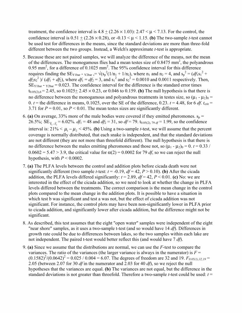
(d) (answers may vary). In the figure below, open circles are the data (offset where needed tominimize overlap). Means are filled circles. Vertical lines indicate 95% confidence intervals..

2. (a) H0: the mean persistence times of the four isolation treatments are equal (µ1 = µ2 = µ3 = µ4) HA: at least one of the means µi is different(b)

Source of variation Sum of squares df Mean squares F-ratio PGroups (treatments) 63.188 3 21.063 3.996 0.035Error 63.250 12 5.271Total 126.438 15

(c) F-distribution with 3 and 12 degrees of freedom. (d) The probability of obtaining an F ratiostatistic as large or larger than the value observed when the null hypothesis is true. (e) The totalsum of squares is the sum of the deviations squared between each observation and the grandmean. The error sum of squares is the sum of the squared deviations between each observationand its group mean. The group sum of squares is the sum of the squared deviations between thegroup mean for each individual and the grand mean. (f) Use R2, the ratio of the group sum ofsquares and the total sum of squares. (g) R2 = 63.188 / 126.438 = 0.50.

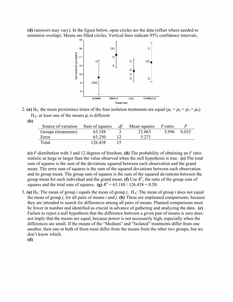
3. (a) H0: The mean of group i equals the mean of group j, HA: The mean of group i does not equalthe mean of group j, for all pairs of means i and j. (b) These are unplanned comparisons, becausethey are intended to search for differences among all pairs of means. Planned comparisons mustbe fewer in number and identified as crucial in advance of gathering and analyzing the data. (c)Failure to reject a null hypothesis that the difference between a given pair of means is zero doesnot imply that the means are equal, because power is not necessarily high, especially when thedifferences are small. If the means of the “Medium” and “Isolated” treatments differ from oneanother, then one or both of them must differ from the means from the other two groups, but wedon’t know which.(d)

(e) The critical value for a t-test has a Type 1 error rate of 0.05 when comparing two means. Thecritical value for the Tukey comparison of all pairs of means is larger so that the probability ofmaking at least one Type 1 error in all the comparisons is only 0.05. (Note that degrees offreedom are 12 in either case because we are using the error mean square to calculate thestandard error of the difference between means).

4. (a) Transformations or a nonparametric Kruskal-Wallis test. (b) The transformation should beattempted first, because this would yield the more powerful test.

5. (a) H0: The mean number of shoots is equal in the three treatments (µ1 = µ2 = µ3). HA: At leastone of the treatment means µi is different.(b)

Source of variation Sum of squares df Mean squares F-ratio PGroups (treatments) 2952.808 2 1476.40 5.32 0.011

Error 8049.067 29 277.55Total 11001.875 31

The critical value is F0.05(1),2,29 = 3.33. Since F > 3.33, P < 0.05, reject H0. Conclude that thereare differences between treatments in mean shoot number. (c) The variable is normallydistributed with equal variance in the three treatment populations. (d) Fixed-effects. The levelschosen were set by the researcher and are repeatable, they were not randomly sampled from apopulation of treatments.

6. (a) 1Y − 2Y = −0.004 − −0.195 = 0.191. MSerror= 0.0345, df = 42, SE = 0.0679, t0.05(2),42 = 2.01,0.054 < µ1 − µ2 < 0.328. (b) Yes, because the study was designed mainly to compare PLP1 geneexpression in persons with schizophrenia to that of control individuals. It was a single focusedcomparison not a broad search for differences between groups. (c) The expression measurementsare normally distributed in the populations with equal variances. (We also assume randomsamples.)

7. (a) H0: Mean PLP1 gene expression is equal in the three groups (µ1 = µ2 = µ3).HA: At least one of the group means µi is different.

Source of variation Sum of squares df Mean squares F-ratio PGroups 0.5403 2 0.2701 7.82 0.0013Error 1.4502 42 0.0345Total 1.9905 44

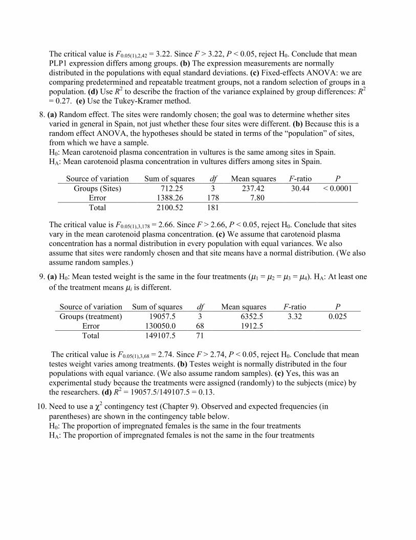
The critical value is F0.05(1),2,42 = 3.22. Since F > 3.22, P < 0.05, reject H0. Conclude that meanPLP1 expression differs among groups. (b) The expression measurements are normallydistributed in the populations with equal standard deviations. (c) Fixed-effects ANOVA: we arecomparing predetermined and repeatable treatment groups, not a random selection of groups in apopulation. (d) Use R2 to describe the fraction of the variance explained by group differences: R2

= 0.27. (e) Use the Tukey-Kramer method.

8. (a) Random effect. The sites were randomly chosen; the goal was to determine whether sitesvaried in general in Spain, not just whether these four sites were different. (b) Because this is arandom effect ANOVA, the hypotheses should be stated in terms of the “population” of sites,from which we have a sample.H0: Mean carotenoid plasma concentration in vultures is the same among sites in Spain.HA: Mean carotenoid plasma concentration in vultures differs among sites in Spain.

Source of variation Sum of squares df Mean squares F-ratio PGroups (Sites) 712.25 3 237.42 30.44 < 0.0001

Error 1388.26 178 7.80Total 2100.52 181

The critical value is F0.05(1),3,178 = 2.66. Since F > 2.66, P < 0.05, reject H0. Conclude that sitesvary in the mean carotenoid plasma concentration. (c) We assume that carotenoid plasmaconcentration has a normal distribution in every population with equal variances. We alsoassume that sites were randomly chosen and that site means have a normal distribution. (We alsoassume random samples.)

9. (a) H0: Mean tested weight is the same in the four treatments (µ1 = µ2 = µ3 = µ4). HA: At least oneof the treatment means µi is different.

Source of variation Sum of squares df Mean squares F-ratio PGroups (treatment) 19057.5 3 6352.5 3.32 0.025

Error 130050.0 68 1912.5Total 149107.5 71

The critical value is F0.05(1),3,68 = 2.74. Since F > 2.74, P < 0.05, reject H0. Conclude that meantestes weight varies among treatments. (b) Testes weight is normally distributed in the fourpopulations with equal variance. (We also assume random samples). (c) Yes, this was anexperimental study because the treatments were assigned (randomly) to the subjects (mice) bythe researchers. (d) R2 = 19057.5/149107.5 = 0.13.

10. Need to use a χ2 contingency test (Chapter 9). Observed and expected frequencies (inparentheses) are shown in the contingency table below.H0: The proportion of impregnated females is the same in the four treatmentsHA: The proportion of impregnated females is not the same in the four treatments

Number of femalesTreatment impregnated not impregnated Row sumoil 14 (12.75) 4 (5.75) 18THC 13 (12.75) 5 (5.75) 18cannabinol 11 (12.75) 7 (5.75) 18cannabidiol 13 (12.75) 5 (5.75) 18Column sum 51 21 72

χ2 = 1.28, df = 3. The critical value is 23),1(05.0χ = 7.81. Since χ2 not greater than 7.81, do not reject

H0. (P = 0.73). We cannot reject the null hypothesis that the proportion of females impregnatedis equal between treatments.

11. Random-effects: the males were chosen at random from the population. A given male is not aspecific, repeatable treatment. The goal is to generalize to the population of males (thehypothesis statements should reflect this). (b) H0: Mean condition of offspring is the same for allmales in the population. HA: Mean condition of offspring differs between males in thepopulation.

Source of variation Sum of squares df Mean squares F-ratio PGroups (males) 9.9401 11 0.9036 4.63 0.0008

Error 4.682 24 0.1951Total 14.622 35

The critical value F0.05(1),11,24 = 2.21 (between 2.18 and 2.25). Since F > 2.21, P < 0.05, reject H0.Conclude that mean offspring conditions differs among males in the beetle population.(c) s2

A = (0.904 − 0.195) / 3 = 0.236. Repeatability = 0.236 / (0.236 + 0.195) = 0.548.

Chapter 161. r = −0.5; r = −0.8; r = 0.5; r = 0.

2. (a) 95%: 0.22 <ρ < 0.63. 99%: 0.14 <ρ < 0.68. (b) 95%: −0.95 <ρ < −0.76. 99%: −0.96 <ρ <−0.70. (c) 95%: −0.17 <ρ < 0.25. 99%: −0.24 <ρ < 0.31

3. (a) Scatter plot:

(b) The relationship is linear, positive, and strong. (c) r = 0.93. SE = 0.13. (d) The standard erroris the standard deviation of the sampling distribution of r. (e) 0.72 < ρ < 0.98

4 (a) No change to the correlation coefficient (r = 0.93). Adding a constant to one of the variablesdoes not alter the correlation coefficient. (b) No change to the correlation coefficient (r = 0.93).Dividing one of the variables by a constant does not alter the correlation coefficient.

5. We can use a paired t-test (Chapter 12).H0: Mean arrival date of male and female partners is the same (µd = 0)HA: Mean arrival date of male and female partners is different (µd ≠ 0)d = 0.3 days (males are slightly earlier on average), SE = 1.667, t = 0.18, df = 9, P = 0.86.t0.05(2),9 = 2.26; since observed t is less than t0.05(2),9, P > 0.05, do not reject H0. Conclude that wecannot reject null hypothesis of equal mean arrival times of males and females. Assume a normaldistribution of differences between arrival rates of males and females.

6. When there is measurement error in one or both of the variables X and Y.

7. A narrower range of values for inbreeding coefficient should lower the correlation with thenumber of surviving pups compared with a wider range of inbreeding coefficients.

8. Use the Spearman rank correlation:H0: The population rank correlation is zero (ρS = 0)HA: The population rank correlation is not zero (ρS ≠ 0)rS = 0.66. P = 0.17.rS (0.05(2),7) = 0.821. Since rS is not greater than or equal to rS (0.05(2),7), P > 0.05, do not reject H0.Conclude that we cannot reject the null hypothesis of zero correlation.(b) Assume random sample and a linear relationship between the ranks of the two variables.

9. Sampling error in the estimates of earwig density and proportion males with forceps means thattrue density and proportion on an island are measured with error. Measurement error will tend todecrease the estimated correlation. Therefore, the actual correlation is expected to be higher onaverage than the estimated correlation.

10. (a) There is a negative linear relationship between telomere length and chronicity, but it is notstrong. (b) −0.43. (c) −0.66 < ρ < −0.13. (d) It is the range of most plausible values for theparameter ρ. If you were to repeatedly and randomly sample individuals from the samepopulation and compute the 95% confidence interval each time, 19 out of 20 of the intervals areexpected to include the population correlation ρ. (e) Assume random sampling, and that the twovariables have a bivariate normal distribution in the population. (f) (Answers may vary) Thescatter plot suggests that the relationship between telomere length and chronicity might be mildlynon-linear, which would violate the assumption of bivariate normality.

11. (a)

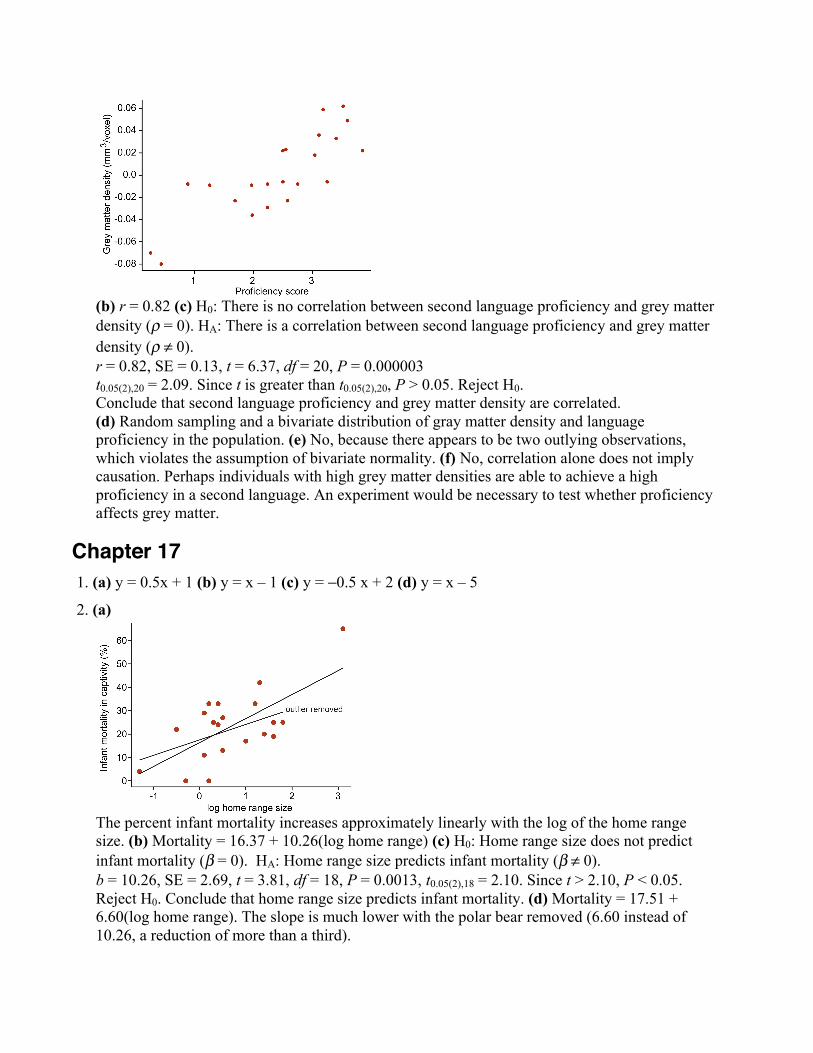
(b) r = 0.82 (c) H0: There is no correlation between second language proficiency and grey matterdensity (ρ = 0). HA: There is a correlation between second language proficiency and grey matterdensity (ρ ≠ 0).r = 0.82, SE = 0.13, t = 6.37, df = 20, P = 0.000003t0.05(2),20 = 2.09. Since t is greater than t0.05(2),20, P > 0.05. Reject H0.Conclude that second language proficiency and grey matter density are correlated.(d) Random sampling and a bivariate distribution of gray matter density and languageproficiency in the population. (e) No, because there appears to be two outlying observations,which violates the assumption of bivariate normality. (f) No, correlation alone does not implycausation. Perhaps individuals with high grey matter densities are able to achieve a highproficiency in a second language. An experiment would be necessary to test whether proficiencyaffects grey matter.

Chapter 171. (a) y = 0.5x + 1 (b) y = x – 1 (c) y = −0.5 x + 2 (d) y = x – 5

2. (a)

The percent infant mortality increases approximately linearly with the log of the home rangesize. (b) Mortality = 16.37 + 10.26(log home range) (c) H0: Home range size does not predictinfant mortality (β = 0). HA: Home range size predicts infant mortality (β ≠ 0).b = 10.26, SE = 2.69, t = 3.81, df = 18, P = 0.0013, t0.05(2),18 = 2.10. Since t > 2.10, P < 0.05.Reject H0. Conclude that home range size predicts infant mortality. (d) Mortality = 17.51 +6.60(log home range). The slope is much lower with the polar bear removed (6.60 instead of10.26, a reduction of more than a third).

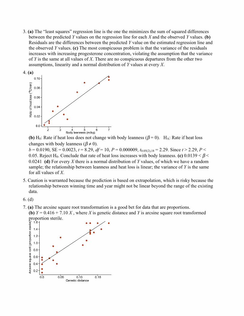
3. (a) The “least squares” regression line is the one the minimizes the sum of squared differencesbetween the predicted Y values on the regression line for each X and the observed Y values. (b)Residuals are the differences between the predicted Y value on the estimated regression line andthe observed Y values. (c) The most conspicuous problem is that the variance of the residualsincreases with increasing progesterone concentration, violating the assumption that the varianceof Y is the same at all values of X. There are no conspicuous departures from the other twoassumptions, linearity and a normal distribution of Y values at every X.

4. (a)

(b) H0: Rate if heat loss does not change with body leanness (β = 0). HA: Rate if heat losschanges with body leanness (β ≠ 0).b = 0.0190, SE = 0.0023, t = 8.29, df = 10, P = 0.000009, t0.05(2),18 = 2.29. Since t > 2.29, P <0.05. Reject H0. Conclude that rate of heat loss increases with body leanness. (c) 0.0139 < β <0.0241 (d) For every X there is a normal distribution of Y values, of which we have a randomsample; the relationship between leanness and heat loss is linear; the variance of Y is the samefor all values of X.

5. Caution is warranted because the prediction is based on extrapolation, which is risky because therelationship between winning time and year might not be linear beyond the range of the existingdata.

6. (d)7. (a) The arcsine square root transformation is a good bet for data that are proportions.

(b) Y = 0.416 + 7.10 X , where X is genetic distance and Y is arcsine square root transformedproportion sterile.

(c) 5.67 < β < 8.52

8. (a) Such a complicated curve is unwarranted by the data. It would do a poor job of predictingnew observations because it does not describe a general trend. A curve fit should be as simple aspossible. (b) First try to transform the data to make the relationship linear. If that fails, considernon-linear regression.

9. (a) b = 11.68, SE = 4.85. (b) −4.08 < β < 27.43 (c) The range of most plausible values for theparameter. In 99% of random samples, the confidence interval will bracket the population valuefor the slope. (d) Measurement error in the X variable (bite force) will tend to lead to anunderestimation of the population slope. (e) Measurement error in the Y variable (territory area)will not bias the estimate of slope (though it will increase its uncertainty).

10. (a)Source of variation Sum of squares df Mean squares F-ratioRegression 194.3739 1 194.3739 5.8012Residual 301.5516 9 33.5057Total 495.9255 10

(b) H0: The slope of the regression of territory area on bite force is zero (β = 0). HA: The slope ofthe regression of territory area on bite force is not zero (β ≠ 0).F = 5.8012, df = 1,9, P = 0.039. F0.05(1),1,9 = 5.12. Since F > 5.12, P < 0.05. Reject H0. Concludethat the slope is not zero (it is positive).(c) That the relationship between X and Y is linear; for each X there is a normal distribution of Yvalues in the population, of which we have a random sample; the variance of Y is the same at allvalues of X. (d) The variance of the residuals. (e) R2 = 0.392. It measures the fraction of thevariation in Y that is explained by X.

11. (a) Perform the analysis with and without the outlier included in the data set to determinewhether it has an influence on the outcome. If it has a big influence, then it is probably wise toleave it out and limit predictions to the range of X values between 0 and about 200 (and urgethem to obtain more data at the higher X values.) (b) Confidence bands give the confidenceinterval for the predicted mean time since death for a given hypoxanthine concentration. (c)Confidence bands. (d) The prediction interval, because it measures uncertainty when predictingthe time of death of a single individual.

12. (a)

(b) The assumptions of equal variance of residuals, and of a normal distribution of Y values ateach X, are not met because of the presence of an outlier. (c) A transformation of the data mightimprove matters, but success is doubtful. Alternatively, use nonparametric correlation to measureassociation between the two variables.

Chapter 181. (a) HOURS = CONSTANT + MUTANT.

HOURS is hours of resting. CONSTANT is the grand mean. MUTANT is the effect of each linesof mutant flies. (b) HOURS = CONSTANT (c) Long horizontal line indicates the grand mean,which is the predicted value for the mean of each group under the null hypothesis. The shorthorizontal lines give the group means, which are the predicted values under the “full” generallinear model including the MUTANT term.

(d) F.2. (a) Plasma corticosterone concentration (b) Chick age group and disturbance regime (c) That the

two explanatory variables interact to affect corticosterone concentrations. (d) Observational. Thepenguins were not assigned by the researcher to age groups or disturbance regimes. (e) Yes.Every combination of the two factors (age group and disturbance regime) is included in thedesign.

3. (a) CORTICOSTERONE = CONSTANT + AGE + DISTURBANCE + AGE*DISTURBANCE.CORTICOSTERONE is the corticosterone concentration, CONSTANT is the grand meancorticosterone concentration, AGE is the age group of the penguin, DISTURBANCE indicateswhether the penguin lived in the undisturbed or tourist-disturbed area, andAGE*DISTURBANCE is the interaction between age and disturbance. (b) H0: Penguin agegroup has no effect on mean corticosterone concentration. H0: Disturbance regime has no effecton mean corticosterone concentration. H0: There is no interaction between penguin age groupand disturbance regime.(c) Penguins were randomly samples from each area and each age class. Corticosteroneconcentrations are normally distributed within age class and disturbance regime. The variance ofthe corticosterone concentration is the same for each combination of age and disturbance.

4. Three of the following: a) To investigate the effect of more than one variable with the sameexperimental design; b) To include the effects of blocking in an experimental design; c) Toinvestigate interactions between the effects of different factors; d) To control for the effects of aconfounding variable by including it as a covariate.

5. In these plots, different symbols refer to different groups of factor B.

6. (a) MEMORY = CONSTANT + LESION. MEMORY is the spatial memory score of a rat,CONSTANT is a constant indicating the value of MEMORY when LESION is zero (Y-intercept), and LESION is the extent of the lesion. (b) MEMORY = CONSTANT (c) The linehaving negative slope in the following graph represents the predicted values from the “full”general linear model. The flat (horizontal) line represents the predicted values under the nullmodel.

7. (a)

(b) EXPRESSION = CONSTANT + WORKERTYPE + BLOCK.EXPRESSION is the for gene expression, CONSTANT is the grand mean of for geneexpression, WORKERTYPE is the worker type, and BLOCK identifies which colony the beecomes from. (c) EXPRESSION = CONSTANT + BLOCK (d) Fixed effect, because the typesare repeatable and of direct interest. The worker types in the analysis are not randomly sampledfrom a population of worker types. (e) Blocking variables allow extraneous variation caused bythe block variable to be accounted for in the analysis and eliminated. When a block variable isincluded, the error variance is smaller, making it easier to detect real effects of the factor.

Chapter 191. (a) For example: Singleton: 3.5, 3.5, 2.6, 4.4 Twin: 3.4, 4.2, 3.4 (b) Singleton: 3.5, 4.2, 4.4, 3.4

Twin: 2.7, 2.6, 1.7 (c) In a bootstrap replicate, the data for each group is a sample of thedata from that same group. Sampling is with replacement (some points might not occur and

others might occur more than once). In a randomization replicate, the data for each group issampled from all the data without regard to original group. Sampling is without replacement(every data point occurs exactly once). (d) No.

2. (a) Yes − by chance the randomization might reassign data to correct groups. (b) Yes. (c) No −Sample sizes of groups must be the same in each randomization as in the data. (d) No − Eachdata point can occur only once in a randomization. (e) No − 3.8 is not in the data. (f) No − Eachdata point can occur only once in a randomization.

3. (a) Yes − by chance bootstrap samples might contain the same observations as the data. (b) No −The bootstrap sample for a group can contain only data from that group. (c) No − Sample sizesof groups must be the same in each randomization as in the data. (d) Yes (e) No − 3.8 is not inthe data (f) Yes.

4. 10.20 < µ < 10.40

5. B is the real data. In A, there is little or no relationship between the two variables, whereas Bshows a strong relationship. Since randomization tends to break up associations, it is more likelythat B is the data and A is a randomization.

6. (a) A comes from randomization and B comes from the bootstrap. (b) Approximately 10 units.The range from X=10 to X=50 should span about 4 standard deviations of the distribution, so 1standard deviation should be about 10 units.

7. (a) The null distribution for the ratio. (b) H0: Mean ratio of range size equals that expected of arandomly broken stick. HA: Mean ratio of range size differs from that expected of a randomlybroken stick. P is approximately 2 × (42/10,000) = 0.0084. Since P < 0.05, reject H0. Concludethat mean ratio in birds exceeds that expected from a randomly broken stick.

8. (a) 98. (b) 100. (c) “Giant pandas are most closely related to bears”9. (a) For example:

Group A Group B7.8 4.5 2.1 12.4 8.9 8.97.8 7.8 4.5 12.4 12.4 12.44.5 2.1 7.8 8.9 8.9 12.47.8 2.1 4.5 10.8 12.4 10.87.8 2.1 4.5 12.4 8.9 10.87.8 4.5 7.8 8.9 10.8 10.84.5 4.5 7.8 10.8 12.4 8.92.1 7.8 4.5 8.9 8.9 10.84.5 7.8 4.5 10.8 10.8 12.42.1 7.8 7.8 8.9 12.4 12.4

(b) Difference in median (B minus A) for these 10 bootstrap replicates:3.0, 4.4, 4.4, 4.4, 4.6, 4.6, 6.3, 6.3, 6.3, 6.34.4 < difference between population medians < 6.3

10. (a) For example:Group A Group B

8.9 2.1 4.5 10.8 7.8 12.44.5 8.9 2.1 7.8 10.8 12.44.5 12.4 2.1 7.8 8.9 10.84.5 8.9 2.1 10.8 12.4 7.8

10.8 4.5 2.1 8.9 12.4 7.84.5 10.8 2.1 12.4 8.9 7.88.9 12.4 4.5 2.1 7.8 10.8

12.4 10.8 2.1 7.8 4.5 8.92.1 10.8 7.8 8.9 12.4 4.57.8 4.5 10.8 12.4 2.1 8.9

(b) H0: The two groups have the same median. HA: The two groups do not have the same medianTest statistic: observed difference between medians (B minus A) = 6.3Null distribution: −3.0, −1.1, 1.1, 1.1, 4.4, 4.4, 4.4, 6.3, 6.3, 6.33 out of 10 outcomes is greater than or equal to the observed value, 6.3P is approximately 2 × 3/10 = 0.6. Since P > 0.20, do not reject H0.Conclude that the null hypothesis of no difference between medians is not rejected.

11. Yes.12. Yes.

13. 10.4 seconds.14. Welch’s approximate t-test.

15. (a) A randomization test. The variable “shell volume” has been kept fixed and values of thesecond variable are all included but in random order. (b) A bootstrap estimate. Each row of thedata set is a different individual sampled from the original sample of individuals. Sampling iswith replacement because the same individual sometimes occurs more than once. (c) The linearcorrelation coefficient, r.

Chapter 20

1. (a) Binomial distribution with n = 47. (b) [ ] ( )3512 11247

tesheterozygo 12| pppL −⎟⎟⎠

⎞⎜⎜⎝

⎛= . It measures

the probability of getting 12 heterozygotes (the data) given that the true value of the proportion

of heterozygotes is p. (c) [ ] ]1ln[35]ln[121247

lnln pppL −++⎥⎦

⎤⎢⎣

⎡⎟⎟⎠

⎞⎜⎜⎝

⎛= . (d) –7.90

2. (a) 0.26 (b) 0.14 < p < 0.40

3. (a) The log of the probability of the DNA data given different possible times since the splitbetween Neanderthals and modern humans. (b) 710 thousand years (c) 470 < time since split <1000 (in thousands of years) (d) This interval is like a 95% confidence interval. It describes themost plausible values of the time since the split between human and Neanderthals.

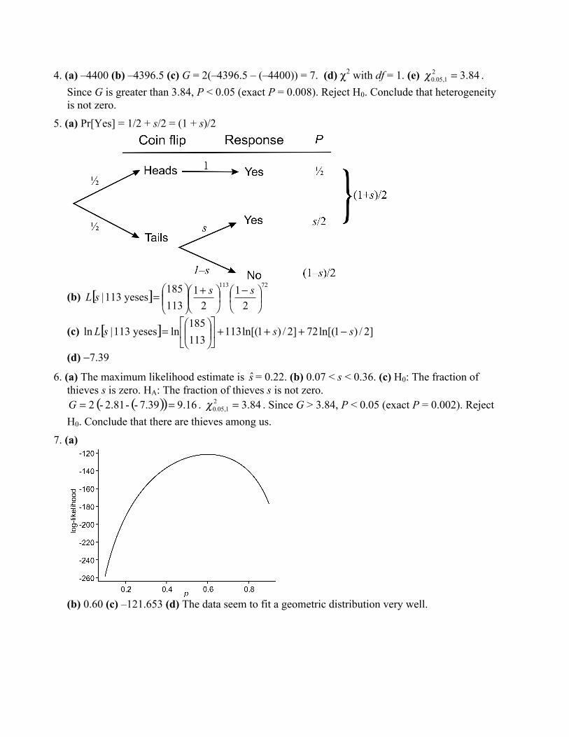
4. (a) –4400 (b) –4396.5 (c) G = 2(–4396.5 – (–4400)) = 7. (d) χ2 with df = 1. (e) 84.321,05.0 =χ .

Since G is greater than 3.84, P < 0.05 (exact P = 0.008). Reject H0. Conclude that heterogeneityis not zero.

5. (a) Pr[Yes] = 1/2 + s/2 = (1 + s)/2

(b) [ ]72113

21

21

113185

yeses 113| ⎟⎠⎞⎜

⎝⎛ −

⎟⎠⎞⎜

⎝⎛ +⎟⎟⎠

⎞⎜⎜⎝

⎛= sssL

(c) [ ] ]2/)1ln[(72]2/)1ln[(113113185

lnyeses 113|ln sssL −+++⎥⎦

⎤⎢⎣

⎡⎟⎟⎠

⎞⎜⎜⎝

⎛=

(d) −7.39

6. (a) The maximum likelihood estimate is s = 0.22. (b) 0.07 < s < 0.36. (c) H0: The fraction ofthieves s is zero. HA: The fraction of thieves s is not zero.

( )( ) 16.97.39--2.81- 2 ==G . 84.321,05.0 =χ . Since G > 3.84, P < 0.05 (exact P = 0.002). Reject

H0. Conclude that there are thieves among us.7. (a)

(b) 0.60 (c) –121.653 (d) The data seem to fit a geometric distribution very well.

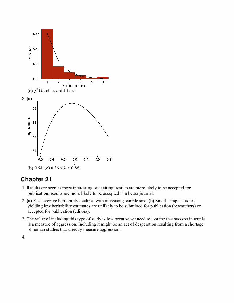
(e) χ2 Goodness-of-fit test

8. (a)

(b) 0.58. (c) 0.36 < λ < 0.86

Chapter 211. Results are seen as more interesting or exciting; results are more likely to be accepted for

publication; results are more likely to be accepted in a better journal.2. (a) Yes: average heritability declines with increasing sample size. (b) Small-sample studies

yielding low heritability estimates are unlikely to be submitted for publication (researchers) oraccepted for publication (editors).

3. The value of including this type of study is low because we need to assume that success in tennisis a measure of aggression. Including it might be an act of desperation resulting from a shortageof human studies that directly measure aggression.

4.

5. (Answers will vary).6. The smaller effect size with larger studies suggests that there is a publication bias affecting the

estimates: small studies yielding low effect sizes are less likely to be appear in the publishedliterature.

7. Even if H0 is true, some studies might reject it by chance. If these are the only studies availablefor review (because of publication bias), then meta-analysis would conclude that H0 is false.

The Analysis of Biological Data - Whitlock and Schluter Solutions to practice problems ... ·...

Documents

Transcript of The Analysis of Biological Data - Whitlock and Schluter Solutions to practice problems ... ·...