THE ALBERTA AIR INFILTRATION MODEL - AIVC · THE ALBERTA AIR INFILTRATION MODEL LS. Walker and D.J....
48
ft' 5 AIM-2 THE ALBERTA AIR INFILTRATION MODEL LS. Walker and D.J. Wilson The University of Alberta Department of Mechanical Engineering Report 71 Jauary 1990
Transcript of THE ALBERTA AIR INFILTRATION MODEL - AIVC · THE ALBERTA AIR INFILTRATION MODEL LS. Walker and D.J....
ft'5
AIM-2
THE ALBERTA AIR INFILTRATION MODEL
LS. Walker and
D.J. Wilson
The University of Alberta Department of Mechanical Engineering
Report 71
Jauary 1990
Nomenclature . .
Acknowledgments
Sununary
Introduction
TABLE OF CONTENTS
Describing the Leakage Distribution
Superposition of Wind and Stack Effects
Comparison of AIM-2 With Other Flow Models
AIM-2 Stack Effect-No Flue
AIM-2 Wind Effect-No Flue
AIM-2 Stack Effect-With Flue
AIM-2 Wind Effect - With Flue
Adjusting Windspeed for Local Terrain
Shelter Coefficients
Validation of AIM-2 and Comparison with Other Models
Effect of Changing Leakage Distribution on Model Predictions
Conclusions
References .
List of Figures
Page
i
iv
v
1
2
3
5
7
9
11
13
14
16
18
24
25
26
27
Nomenclature
Ao
f3
{3f
f3o
B1
c
Cc
Cf
cflue
Cw
AP
AP ref
AT
F
fs
f s,LBL
fw
g
H
Hf
M
n
Pm
Ps
Ps
Pw
Equivalent leakage area
Dimensionless Flue Height
Dimensionless Flue Height
Dimensionless neutral level height
Interaction coefficient for combining wind and stack effect
Building leakage coefficient
Ceiling leakage
Floor leakage
Flue leakage
Wall leakage
Pressure difference
Reference pressure difference for effective leakage area
Indoor-Outdoor temperature difference
Factor used to determine stack flow factor, fs
Stack flow factor
LBL stack flow factor
Wind flow factor
Gravitational acceleration
Building eave height
Height of flue top
Factor used to determine stack flow factor, fs
Building leakage exponent
Windspeed exponent at met . station
Windspeed exponent at building site
Stack effect reference pressure
Wind effect reference pressure
i
Q Total flow through building envelope
Qs Flow due to stack effect
Qw Flow due to wind effect
O h 1
d Flow due to wind effect for a sheltered building 'w, s e tere
O h 1
d Flow due to wind effect for an unsheltered building 'w,uns e tere
R Ceiling-floor leakage sum
R* Parameter used to determine f WC
Po Outdoor air density
S Factor used to determine wind flow factor, fw
Sw Local wind shelter coefficient
S Shelter coefficient for building walls WO
S fl Shelter coefficient for top of flue w ue
Ti Indoor temperature
T0 Outdoor temperature
U Windspeed
Ue Unobstructed windspeed at eaves height at the building site
U t Windspeed recorded at met. station me
U h 1 d Effective sheltered windspeed s e tere
U h 1 d Effective unsheltered windspeed uns e tere
X Ceiling-floor leakage difference
Xe Critical value of X at which the neutral level passes through the ceiling
x . crit
Xs
x*
y
Critical value of X for wind flow factor with a crawl space, f
WC
Shifted X value for wind flow factor with a crawl space, f
WC
Parameter used to determine f WC
Fraction of building leakage in the flue
ii
y*
z
Zm
Zo
Parameter used to determine f WC
Height above grade level
Height at which met. station wind is measured
Terrain roughness scaling length
iii

Acknowledgments and Liability Disclaimer
The model development and testing reported here was supported by
research grants from the Natural Sciences and Engineering Research
Council, Energy Mines and Resources Canada, and the Alberta/Canada Energy
Resources Research Fund (A/CERRF) to D.J. Wilson, and by a grant-in-aid
from the American Society of Heating, Refrigerating and Air Conditioning
Engineers to I.S. Walker.
The models and methods in this report were developed for scientific
study purposes. The University of Alberta and the authors accept no
liability for errors or omissions or interpretation in its use.
A/CERRF is a joint program of the Government of Canada and the
Government of Alberta, administered by Alberta Energy and Natural
Resources. Neither the Government of Alberta nor its officers, employees
or agents makes any warranty in respect of this report or its contents.
iv
Summary
This report presents the relevant equations needed for a complete
single zone air infiltration model (AIM-2), and validates the model by
comparing its predictions to measured infiltration rates in test houses.
The pressure-flow relationship for the building envelope is described
using a power law whose coefficients are determined by fan pressurization
testing. Unlike other simple models the furnace flue is treated as a
separate leakage site.
Wind and stack effects are determined separately, then superposed as
a sum of pressures, with a correction term that accounts for the
interaction of wind and stack induced pressure. This wind and stack
effect interaction term includes the only empirical constant in AIM-2
determined by fitting to measured data.
The predictions of AIM-2 have been compared to those of four other
simple models, and to infiltration data measured in two houses at the
Alberta Horne Heating Research Facility (AHHRF). The results indicate that
treating the furnace flue as a separate leakage site significantly
improves model predictions. Because the flue leakage is at a different
height for stack effect AIM-2's predictions have about 5% error and the
other model errors range from about 20% to 50% . The flue top has its own
wind pressure coefficient, and is allowed to have different shelter than
the rest of the building. For a sheltered building with a flue AIM-2's
error is about 16% with the other models ranging from about 40% to 90%.
For an unsheltered building with a flue AIM-2 has an error of about 12%
with the other models ranging from about 20% to 26%. These errors are the
approximate sum of the bias and scatter in each case. The measurements
also show that the orifice flow assumption used in some models is a
significant source of error, and the power law pressure-flow relationship,
used in AIM-2, is more appropriate as it reduces the scatter error for a
house with no flue from 18% for an orifice flow model to 3% for AIM-2.
The two major sources of uncertainty in applying AIM-2 are the
estimation of local wind shelter and leakage distribution. Building
shelter is difficult to estimate due to the complexity of local air flow
around buildings. The table of shelter values for AIM-2 defines shelter
coarsely and any finer selections of shelter would be difficult to
justify. The leakage distribution between walls, floor, ceiling and flue
v
was estimated by visual inspection. It is shown that errors in estimating
this leakage distribution can cause significant errors in predicting air
infiltration.
vi
Introduction
The pressure differences that cause air infiltration are generated by
the natural effects of wind (wind effect) and indoor-outdoor temperature
difference (stack effect). In a real building the pressure acting across
a specific leakage site is a combination of all three effects. An air
infiltration flow model is used to find the total ventilation rate for a
building from weather data, using the building's leakage distribution,
pressure-flow and wind shelter characteristics.
The purpose of this report is to present the relevant equations
needed for a complete single zone model, and then validate the model by
comparing its predictions to measured ventilation rates in real buildings.
This report will not go into great detail about equation derivations and
justification of assumptions, or provide an extensive literature review.
In order to develop a simple model for estimating air infiltration it
is necessary to examine separately the flowrate through each leak
resulting from stack and wind effects. To determine the total building
infiltration rate the building leakage flow pressure characteristic must
be known. Fan pressurization tests used to find this flow characteristic
have shown that the assumption of orifice flow used in the most popular
infiltration models is unrealistic. A better way of describing the
pressure-flow relationship for a building envelope is the power law
Q - Ct.Pn (1)
where C and n are found from least squares fitting to pressurization test
results. For orifice flow n-1/2, but for a typical residential building
n=2/3. Measurements by the authors on several test houses have
demonstrated that a single value for C and n accurately describe building
leakage flows over a wide pressure range, from less than 1 Pa to over 50
1
Pa. Typical wind and stack effect pressures lie in the range from 1 Pa to
10 Pa.
The experimentally determined C and n are used in separate
relationships to find stack and wind induced flow rates. The Alberta
Infiltration Model, Version 2 (AIM-2) gives improved estimates for total
building ventilation rates of single zone houses with furnace flues. This
improvement is obtained by incorporating the Q - c~pn characteristic into
the model from first principles, and by treating the flue as a separate
leakage site with its own wind shelter, locating the flue outlet above the
house (depending on the actual flue height) rather than grouping the flue
leakage with the other building leaks, as in other models.
Describing the Leakage Distribution
Pioneering work by Sherman (1980) introduced the idea of using a set
of quantitative parameters to describe the leakage distribution of the
building envelope, and to determine the stack-driven and wind-driven flow
rates in terms of stack and wind factors, fs and fw. These two factors
contain all the information about how the leakage distribution affects the
total building infiltration. The leakage distribution is specified in
terms of the ratio parameters R, X and Y, calculated from the leakage
coefficients of each of the following components.
cflue
Cc
Cf
leakage of flue at elevation z - Hf above floor level
leakage of ceiling at elevation z - H above floor level
leakage of floor level leaks, at z = 0
2
3
Cw = leakage of walls, (Each of the four walls is assumed to
have the same uniformly distributed leakage)
Assuming that the exponent n in (1) is the same for all leakage sites, the
total leakage coefficient C is
C - Cc + Cf + Cw + Cflue (2)
Leakage distribution parameters are defined using the format suggested by
Sherman (1980), with the addition of a separate flue fraction for AIM-2.
c c + cf R - c "ceiling-floor sum" (3)
c c - cf x - c "ceiling-floor difference" (4)
c y _ flue
c "flue fraction" (5)
Superposition of Wind and Stack Effects
In real infiltration the stack and wind effects are not independent,
because wind and stack pressures act simultaneously across each leak. The
magnitude of this pressure difference depends on the internal pressure of
the building, which is set by the requirement that total mass inflow must
equal the total mass outflow. The variation in stack induced pressure
difference with height above the floor gives rise to a location on the
building envelope where there is no pressure difference between indoors
and outdoors. This neutral pressure level depends on the leakage
distribution, and can be calculated for the case of stack induced
infiltration with no wind. When wind pressures are present the neutral
level shifts (and is different for each wall) in order to keep the total
inflow and outflow equal. The internal pressure then depends on both the
wind and stack pressures, and wind and stack flowrates cannot simply be
added, but instead must be superposed in some way that accounts for this
interaction.
The superposition technique used in AIM-2 adds the two flows non-
linearly, as if their pressure differences added, and introduces an extra
term to account for the interaction of the wind and stack effects in
producing the internal pressure. The AIM-2 model uses a simple first-
order neutral pressure level shift that produces the superposition
1 1 1
Q - (Q~ +~ + Bl (Qs~)2n )n (6)
where Qs Flow due to stack effect
Qw - Flow due to wind effect
Q - Total flow due to combined wind and stack effects
Bi - Interaction coefficient, assumed constant
It is easy to show that the interaction term causes the largest percentage
effect on Q when wind and stack flows Qw and Qs are equal. The constant
B1 was determined empirically using direct measurements of air
infiltration. Analysis of data from several houses at the Alberta Home
Heating Research Facility for periods where Q8 and Qw were approximately
equal suggests that a reasonable estimate for B1 is
1 B1 ""' - 3
4
from which we see that wind and stack effect interaction reduces the total
infiltration rate from the level predicted by a simple sum of pressures
superposition. This is the only constant in AIM-2 that was determined by
fits to measured data. The other empirical inputs to AIM-2 are the set of
wind pressure coefficients from Akins (1979) wind tunnel experiments, the
flue cap pressure coefficient from Hayson and Swinton (1987), and our
estimates of wind shelter coefficients. Model validation, discussed
later, used data sets (from the Alberta Home Heating Research Facility)
chosen to be dominated by wind or stack effects, so that interaction term
in (6) involving the empirical coefficient B1 was negligible. In this
way, AIM-2 could be tested against independent infiltration measurements
that played no part in its development.
Comparison of AIM-2 With Other Flow Models
The two models that most closely resemble the Alberta Infiltration
Model (AIM-2) use variable leakage distribution. They are Sherman's
orifice flow model fom Sherman and Grimsrud (1980) (often referred to as
the LBL model), and the "Variable n" model, refined by Reardon (1989) from
Yuill's (1985) extension of Sherman's model to power law leakage Q - C~Pn.
The other models chosen for comparison; Shaw (1985) and Warren and Webb
(1980), use empirical coefficients that do not change from house to house.
All the models make the implicit assumption that each of the four walls
has the same leakage. The significant differences between AIM-2 and
Sherman's and Yuill's models are summarized below:
1. The attic space above the ceiling was assumed in Sherman's LBL Model (and in Yuill's extension) to have a zero pressure coefficient. The attic pressure coefficient in AIM-2 is assumed to be a weighted average of the pressure coefficients on the eave and end wall vents, and the roof surface vents. The eave vents are assumed to have the same pressure as the wall they are
5
adjacent to. The eave vents above each wall are assumed to have the same size, and the roof vents to have a size equal to the sum of the eaves.
2 . The floor leakage in Sherman's LBL model (and in Yuill's power law extension) was located above a crawl space which was assumed to have a zero pressure coefficient. In AIM-2 the crawlspace pressure is taken as the average of the four outside wall pressures from wind effect. AIM-2 also deals with a house with a full basement or a slab-on-grade, where "floor" leakage is the crack around the floor plate resting on the foundation, plus cracks, holes and other leakage sites in the concrete foundation above grade. These floor level leakage sites are assumed to be uniformly distributed around the perimeter of the house near ground level, and to be exposed to the same pressure as each of the walls on which they are located.
3 . There is no furnace flue in Sherman's LBL model, or Yuill's power law extension. In these models any furnace flue leakage is simply added to the ceiling leakage, and sees the attic pressure. In AIM-2 the furnace flue is incorporated as a separate leakage site, at a normalized height fif above the floor. (The ceiling of the upper story is at p - 1.0, the floor at P - 0) The flue is assumed to be filled with indoor air at room temperature, and exposed at its top to a pressure set by wind flow around the rain cap.
4 . Sherman's LBL model assumes orifice flow with n - 0.5 in Q - C6Pn of each leak. Both Yuill's extension and the Alberta Infiltration Model AIM-2 assume a single value of n in the range 0.5 to 1.0. (orifice flow to fully developed laminar flow) The same value of n is assumed to apply to each leakage site, floor, walls, and ceiling. The flue is assumed to have a value of n = 0.5 in developing exact numerical solutions for the wind and stack factors. Because these factors are then applied to the single average exponent n for the whole house , fs and fw depend on n in their flue terms. The empirical approximating functions in (21) to (26) reflect this combined n and Y dependence.
5. Both Sherman and Yuill assume that wind flow, Qw, and stack flow Qs, combine in quadrature as a sum of squares. The Alberta Infiltration Model AIM-2 includes the interaction term in (6) which accounts empirically for a wind-induced shift cf the neutral pressure level.
The effect of these different assumptions in AIM-2 is easiest to assess by
first looking at a house without a flue.
6
AIM-2 Stack Effect-No Flue
form
where
The flow induced by stack effect is assumed to have the functional
Q = C f Pn s s s
C = total building leakage coefficient in C6Pn, m3/s Pan
Ps - stack effect reference pressure - Po g H [
g - gravitational acceleration~ 9.8 m/s2
Po - outdoor air density, kg/m3
fs = stack flow factor
) ,Pa
(7)
(8)
H - building eave height (ceiling height of the uppermost story), m
Ti = Indoor Temperature, °K
T0 - Outdoor Temperature, °K
An exact numerical solution was found for fs by balancing inflows and
outflows. For all n values the exact equation for the stack factor (which
requires a numerical solution) with no flue, is the same as Yuill's
(1985). AIM-2 uses an approximating function instead of the exact
solution for stack factor. The functional form of this approximation was
selected to produce the correct behavior of fs at the limits where all
leakage is concentrated in the walls (R - 0), in the floor and ceiling
(R = 1), and for the ceiling-floor difference ratio limits of X = 0 and
X - ±1. The functional form is
fs - [ 1 + nR n+l l [ ~ -_! ( _i ) 5/4ln+l
2 2-R (9)
7
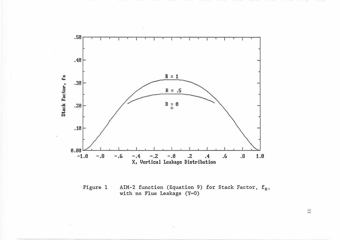
Values of fs from equation (9) are shown graphically in Figure 1, with n -
2/3. Note that fs for R - 0 is a single point at X - 0. When n - 0.5 the
exact numerical solution for the stack flow Qs is the same as Sherman's
LBL model. However, the approximating function recommended by AIM-2 is
somewhat different than Sherman's approximation. Sherman's stack factor
f . s,LBL is defined by
lo. s
Qs - Vs,LBL [ :: (10)
where A0 - leakage area of the house at reference pressure AP f " Setting re
n - 0.5 in equation (7) and equating to (10) yields
[ lo. s
1 - A f P
0 o s,LBL c f
s
At a reference pressure AP f the leakage area A0 and flow coefficient C re
are related by
A - C ~ (AP )n-0.5 (
p )0.5 0 2 ref (11)
so our definition of the stack factor fs is related to the LBL value by
f s
-0.Sf __ 2 s,LtiL
(1 ?) , -- ,
Using (12), Sherman and Grimsrud's (1980) approximating function for
orifice flow may be written in the form
f ( 1 + 0 . SR ) s, LBL ... 1. 5 r 2 r2
} - } ( (2~R) 2 ) (13)
8
We believe (9) with n - 0.5 is a more accurate approximation than the LBL
function in (13).
AIM-2 Wind Effect-No Flue
The wind induced infiltration rate Qw is defined in terms of wind factor
fw by
O ~ C f P n 'w w w
where C has already been defined, and the reference wind pressure is
p w
(S U )2 p ~
0 2
(14)
(15)
Ue - unobstructed wind speed (with no local shelter) at eaves height
at the building site
fw - wind factor
Sw - local wind shelter coefficient
To derive an exact numerical solution for fw, the wind pressure
coefficient data set of Akins (1979) was used, with wind normal to the
upwind wall, and all walls of the same length (square floor plan). The
approximating function developed for AIM-2 to fit the exact numerical
solution is
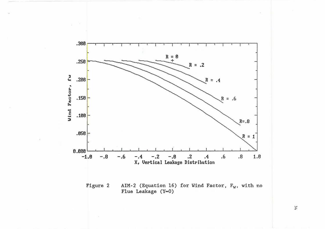
fw - 0.19(2-n) [ 1 _ ( x;R t2] (16)
Both the LBL and AIM-2 models make the implicit assumption that fw does
not change significantly with wind direction. This assumption was checked
by using wind direction dependent pressure coefficients from Akins (1979)
and found to introduce a variability of about± 10%. Three other wind
9
tunnel data sets, ASIIRAE (1989), AIVC (1986) and Wiren (1984), for wall
and roof pressure coefficients were also used to find numerical solutions
for fw. These other sets of pressure coefficients produce wind factors
that are functionally similar, but with a difference in magnitude. The
two extreme results are from Wiren's and ASHRAE's data sets, and these
produce values of fw that are respectively 10-20% larger and 10-20%
smaller compared to the values of fw found using Akins data set.
It is interesting to compare the wind factor fw in (16) with Sherman
and Grimsrud's approximation
2 p 0.5
( w) -A f --~ o w,LBL p0
(17)
Equating this to (14) with Sw - 1.0 for no shielding yields, for n - 0.5
( 2 )0.5 - Af =Cf p o w,LBL w
0
Then, using (11) with n = 0.5 we see
f w,LBL f w (18)
Using (18), Sherman's approximating function is, for no shielding (i.e .
using the largest value for his generalized shielding coefficient)
f w,LBL = 0.324 (1 _ R)l/3 (19)
For all leaks in the walls, R - 0 and X = 0 and n - 0.5, (16) predicts
fw = 0.285, about 10% less than Sherman's value in (19). The assumptions
for floor level and attic pressure coefficients in Sherman's LBL model
10
make (19) independent of the difference factor X between ceiling and floor
level leakage. In AIM-2, there is a strong dependence of fw on X in (16)
caused by our assumptions for attic and floor level pressures. This is
shown graphically in Fig. 2, with n = 2/3.
AIM-2 Stack Effect-With Flue
With a flue, the model becomes more complicated because both the size
and height of the flue are variables in a non-linear flow network.
Numerical solutions to the exact flow balance equation were approximated
by algebraic functions for use in AIM-2. In addition to the distributed
leakage of the building envelope expressed in terms of R, X and Y, we
require the normalized height ~f of the flue,
Where: Hf
Hf /Jf - li
Height of flue top
H - Building eave height
In both the exact numerical solution, and the approximating functions
(20)
developed for AIM-2, the flue is assumed to be filled with air at indoor
room temperature. The air flow induced during combustion when the flue is
hot is neglected.
The stack factor fs in (7) was found by a numerical solution of the
non-linear inflow-outflow balance equations, and is approximated in AIM-2
by the function
f s (
1 +nR ) ( ! _ ! 5 I 4) n+ 1 n+l 2 2 M + F (21)
where
11
M - (X + (2n+l)Y)2
2-R
with a limiting value of
M ~ 1.0
The additive flue function F is,
where
3n-l 3
F - nY(f3 - 1) f
for 2
(X + (2n+l)Y) ~ 1 2-R
for 2
(X + (2n+l)Y) > 1 2-R
[ 1 -3(Xc - X)2Rl - n l
2(/3f + 1)
X - R + 2(1-R-Y) - 2Y(f3 - l)n c n+l f
the variable Xe is the critical value of the ceiling-floor difference
(22)
(23)
(24)
(25)
fraction X at which the neutral level passes through the ceiling in the
exact numerical solution. For X > Xe the neutral level will be above the
ceiling, and attic air will flow in through the ceiling. For X < Xe room
air will exfiltrate through the ceiling. This critical value of Xe is
useful in determining whether moist indoor air will exfiltrate through the
ceiling and cause ice to form in attic insulation in winter. The role of
the flue in reducing ceiling exfiltration is evident from the contribution
of the Y factor in (25).
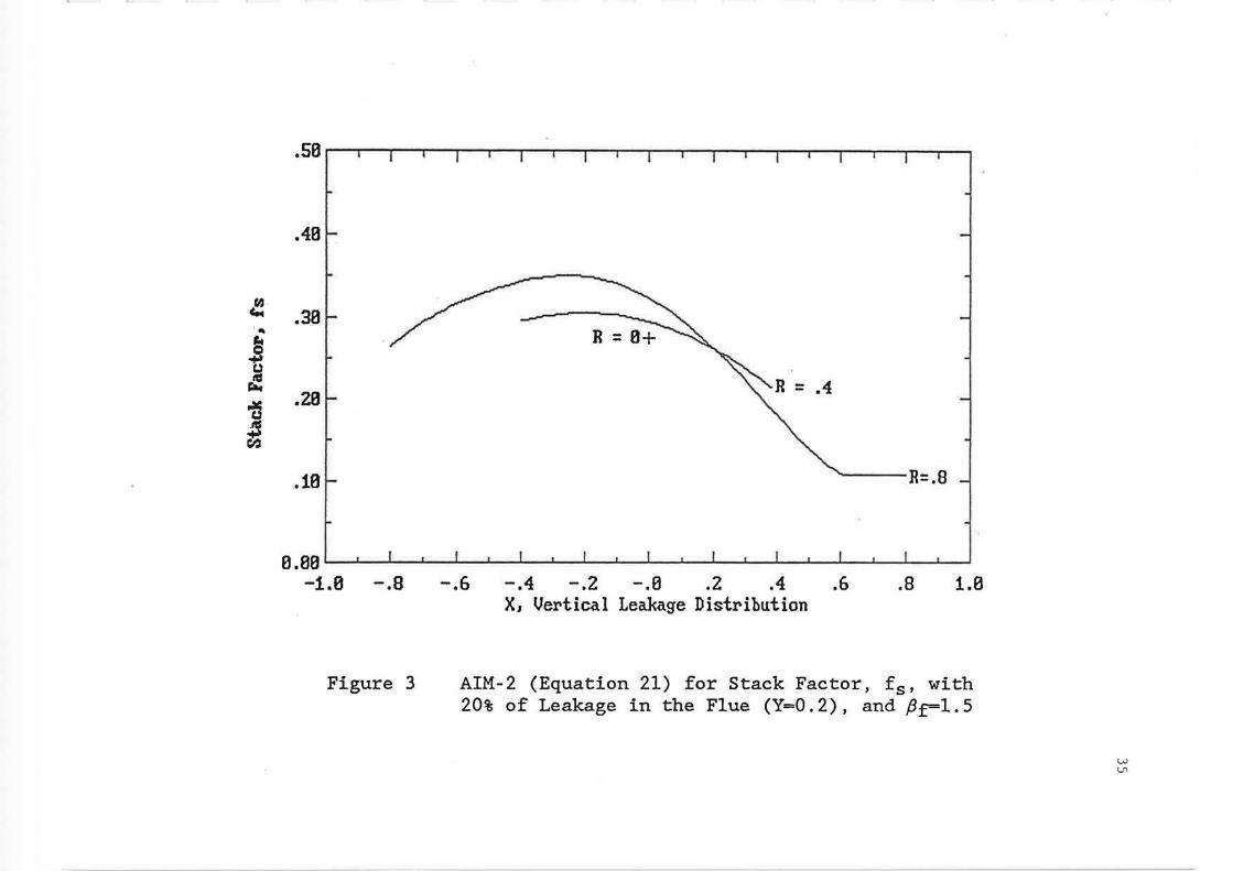
The functions in (21) to (25) reduce to (9) when Y - 0. The stack
factor calculated using equation (21) is shown in Fig. 3 for typical
values of n - 2/3, {3f - 1.5 and Y - 0.2. Treating the flue as a separate
leakage site with a stack height above the ceiling has a significant
effect on the stack factor fs, as can be seen by comparing Fig. 1 and 3.
12
AIM-2 Wind Effect - With Flue
The exact numerical solution for fw, and its approximating function
in AIM-2 depend on the set of wind pressure coefficients used. Using the
pressure coefficients from Akins (1979), the recommended approximating
function for wind factor is
f w
0.19(2-n+ _ (x;Rf/2-Yl
where s - X + R + 2Y 2
~ (S - 2YS4
) (26)
The functional form for fw was chosen to produce the correct behavior for
the limiting values of all leakage concentrated in either walls, floor or
ceiling, and for X - 0 where the floor and ceiling leakage are equal. The
flue height Pf does not appear in (26), because, in the exact solution the
dependence on Pf is felt very weakly through the change in windspeed at
the flue top. When Y - 0 (26) reduces to (16), the relationship for fw,
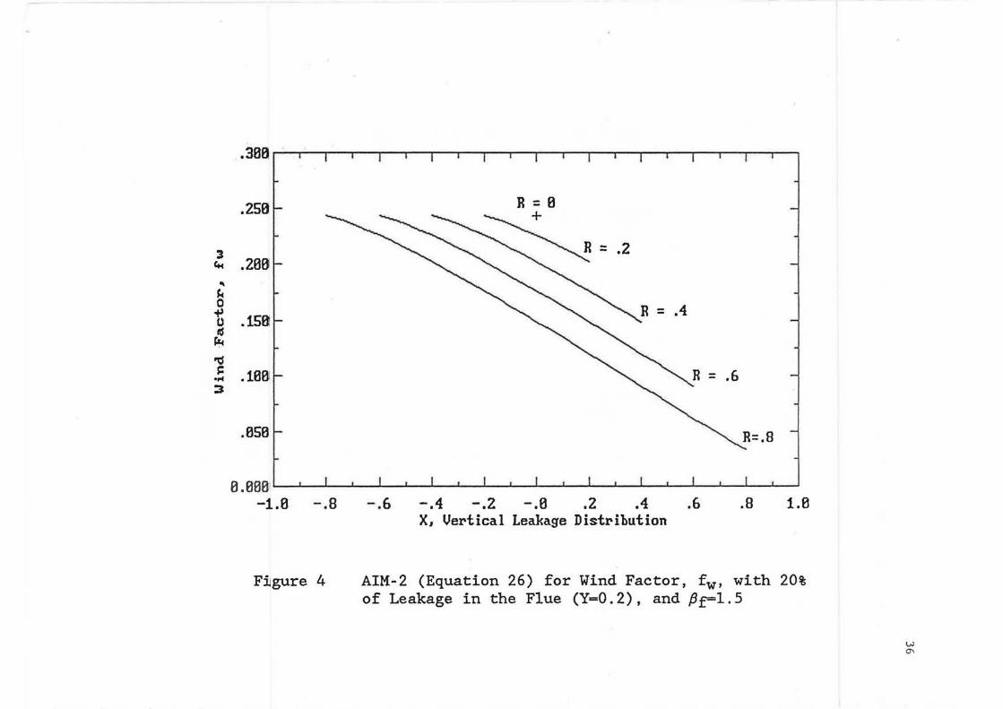
with no flue. The wind factor calculated from equation (26) is shown in
Fig. 4 for n - 2/3, Y - 0.2. Comparing Fig. 2 with no flue to Fig. 4 with
a flue, we see that there is little effect on wind factor fw of
considering the flue leakage as a hole in the ceiling, venting into the
attic, or as a separate leakage site with its own flue cap pressure
coefficient above the roof . We will show later that the major advantage
of the separate flue leakage site is to allow it to have a different wind
shelter than the rest of the building.
For a house with a crawl space, the pressure inside the crawl space
may be approximated by the average of the four walls which change the
dependence of fw on X and R. Using this assumption to find wind factor
13
yields a different empirical approximation, f , for a house with a crawl WC
space,
* * * f - 0.19(2-n) X RY WC
(26a)
where R* = 1 - R( I+ 0.2)
y* = ( 1 - ~)
x* - 1 - [[ ~: ~s)f 75
where ( (1-R) ) _ l.SY x - 5 s
There is a critical value of the floor-ceiling difference fraction, X . , cr1t
above which fw does not change with X,
x crit - 1 - 2Y
If X > X . then use X = X . crit cr1t
For the case where all the leaks are in the walls, R = 0 and the wind
factor for a house with a crawl space is f we 0.276, which is 15% below
Sherman's estimate (19) and 3% less than for a house with no crawl space
(26).
Adjusting Windspeed for Local Terrain
Surrounding buildings, vegetation and terrain produce two types of
wind shelter. Very near the building local obstructions caused by trees
and neighboring structures located within two house heights provide direct
shielding. This important source of wind shielding will be dealt with
14
later by a shelter coefficient. A second type of shelter is provided by
the overall terrain roughness that extends several kilometers upwind of
the buildings. This roughness will change the shape of the wind velocity
profile. Because windspeed is measured at an airport meteorological tower
at a height Zm, usually in open flat terrain, some adjustment is required
to estimate the wind speed at eaves height H in the local building terrain
(neglecting specific nearby obstructions). One simple method of
accounting for these differences in measuring heights (zm and H) and in
terrain roughness is to use a power law profile U ~ zP for mean windspeed
with height above ground. Irwin (1979) gives values of the exponent p for
varying terrain roughness and atmospheric stability classes. Then, if we
assume that the windspeed at the surface influenced boundary layer height
z ~ 600 m is the same above the airport and the building site, the wind
speed at eaves height H is
where
Zm
H-
Pm
Ps Ue
u met
u ~ (6oo)Pm (_!!__)Psu e z 600 met
m
height at which met. station wind is measured, m.
building eaves height above ground
windspeed exponent at met station
wind speed exponent at building site
unobstructed windspeed at building eaves height
windspeed recorded at met. station
The eave height can be estimated from
H ~ 0.5 + 2.5 N
where H is in meters, and N is the number of stories. To simplify the
(27)
(28)
process of estimating wind effects we will reduce Irwin's six stability
15
classes to two by asswning that met. tower windspeeds greater than 3 m/s
occur in neutral stability (class D) and less than 3 m/s are in stable
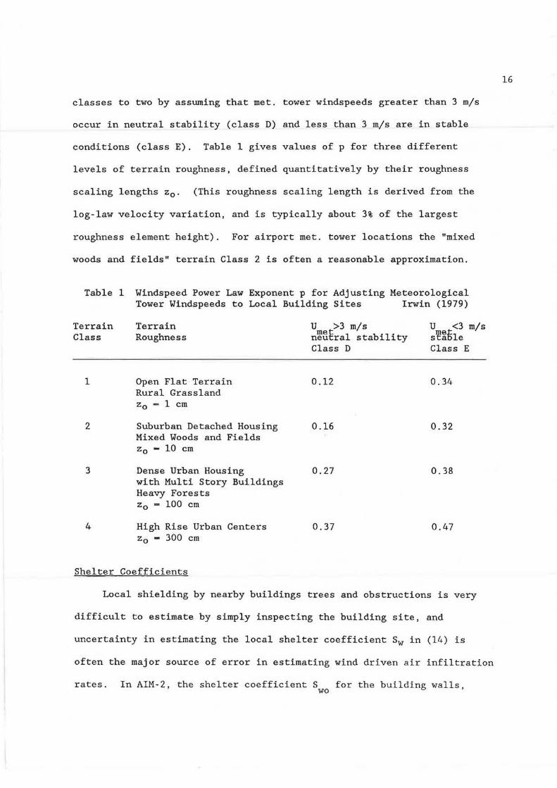
conditions (class E). Table 1 gives values of p for three different
levels of terrain roughness, defined quantitatively by their roughness
scaling lengths z 0 . (This roughness scaling length is derived from the
log-law velocity variation, and is typically about 3% of the largest
roughness element height). For airport met. tower locations the "mixed
woods and fields" terrain Class 2 is often a reasonable approximation.
Table 1 Windspeed Power Law Exponent p for Adjusting Meteorological Tower Windspeeds to Local Building Sites Irwin (1979)
Terrain Class
1
2
3
4
Terrain Roughness
Open Flat Terrain Rural Grassland z0 = 1 cm
Suburban Detached Housing Mixed Woods and Fields z 0 = 10 cm
Dense Urban Housing with Multi Story Buildings Heavy Forests z0 = 100 cm
High Rise Urban Centers z0 - 300 cm
Shelter Coefficients
U >3 m/s n~Stral stability Class D
0.12
0.16
0.27
0.37
U <3 m/s s¥!~Ble Class E
0.34
0.32
0.38
0.47
Local shielding by nearby buildings trees and obstructions is very
difficult to estimate by simply inspecting the building site, and
uncertainty in estimating the local shelter coefficient Sw in (14) is
often the major source of error in estimating wind driven air infiltration
rates. In AIM-2, the shelter coefficient S for the building walls, WO
16
combined with a different coefficient S fl for the top of the flue stack w ue
gives an improved estimate of the total local shielding. A simple linear
combination is used in AIM-2,
s w S (1 - Y) + S fl (l.5Y) wo w ue (29)
where the factor 1.5 is an empirical adjustment found by comparing AIM-2
to an exact numerical solution using local leaks, each with their own
pressure coefficients. S fl - 1.0 for an unsheltered flue, which w ue
protrudes above surrounding obstacles, and S fl - S for a flue top w ue wo
which has the same wind shelter as the building walls. With no
flue, Y - 0 and Sw - S . WO
Due to the difficulty in accurately estimating the effects of local
wind shielding, the proposed values in Table 2 give only a rough
approximation for the shelter coefficient. This table uses the shielding
class description suggested by Sherman and Grimsrud (1980), with the
addition of a new class of "complete shielding". However, it is important
to note that although the terrain classes are the same, the values for S WO
suggested in AIM-2 are not the same as Sherman and Grimsrud's "generalized
shielding coefficient" used in the LBL and variable n models.
17
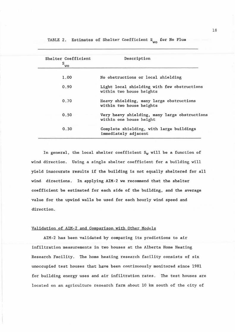
TABLE 2. Estimates of Shelter Coefficient S for No Flue WO
Shelter Coefficient s
WO
1.00
0.90
0.70
0.50
0.30
Description
No obstructions or local shielding
Light local shielding with few obstructions within two house heights
Heavy shielding, many large obstructions within two house heights
Very heavy shielding, many large obstructions within one house height
Complete shielding, with large buildings immediately adjacent
In general, the local shelter coefficient Sw will be a function of
wind direction. Using a single shelter coefficient for a building will
yield inaccurate results if the building is not equally sheltered for all
wind directions. In applying AIM-2 we recommend that the shelter
coefficient be estimated for each side of the building, and the average
value for the upwind walls be used for each hourly wind speed and
direction.
Validation of AIM-2 and Comparison with Other Models
AIM-2 has been validated by comparing its predictions to air
infiltration measurements in two houses at the Alberta Home Heating
Research Facility. The home heating research facility consists of six
unoccupied test houses that have been continuously monitored since 1981
for building energy uses and air infiltration rates. The test houses are
located on an agriculture research farm about 10 km south of the city of
18

Edmonton, and are situated in a closely spaced east-west line with about
2.8 m separation between their side walls. False end walls, with a height
of 3.0 m but without roof gable peaks, were constructed beside the end
houses (houses 1 and 6) to provide equivalent wind shelter and solar
shading. Construction details are given in Table 3 for houses 4 and 5
used in the validation study reported here.
The flat exposed site is surrounded by rural farmland, whose fields
are planted with forage and cereal crops in swnmer, becoming snow-covered
stubble in winter. Windbreaks of deciduous trees cross the landscape at
intervals of a few kilometers, with one such windbreak located about 240 m
to the north of the line of houses. The houses are totally exposed to
south and east winds. Several single-story farm buildings, located about
50 m to 100 m to the west, provide some shelter from west to northwest
winds.
Micrometeorological towers are located midway along the row of houses
on both the north and south sides of the line of houses. The wind speed
and direction at a 10 m height are measured with low friction cup
anemometers and vanes on both towers. The tower windspeed accounts for
local terrain effects, including the shelter from farm buildings and local
windbreaks. These on-site measurements require only a correction for
tower to eaves height, so that Pm - Ps - 0.16 was used in (27), with
H - 3 m and Zm - 10 m.
Continuous infiltration measurements were carried out in the six test
houses using a constant concentration SF6 tracer gas injection system in
each house. Two independent infrared analyzers sampled three houses in
sequence through a manifold controlled by solenoid valves, as described in
Wilson and Dale (1985). It is important to note that the measured data
19
were not used to adjust any model coeffi dents, except to find a suitable
value for B1. The validation carried out here used data sets with stack
and wind dominated extremes, so that determining B1 from the measured data
had a negligible effect on model validation.
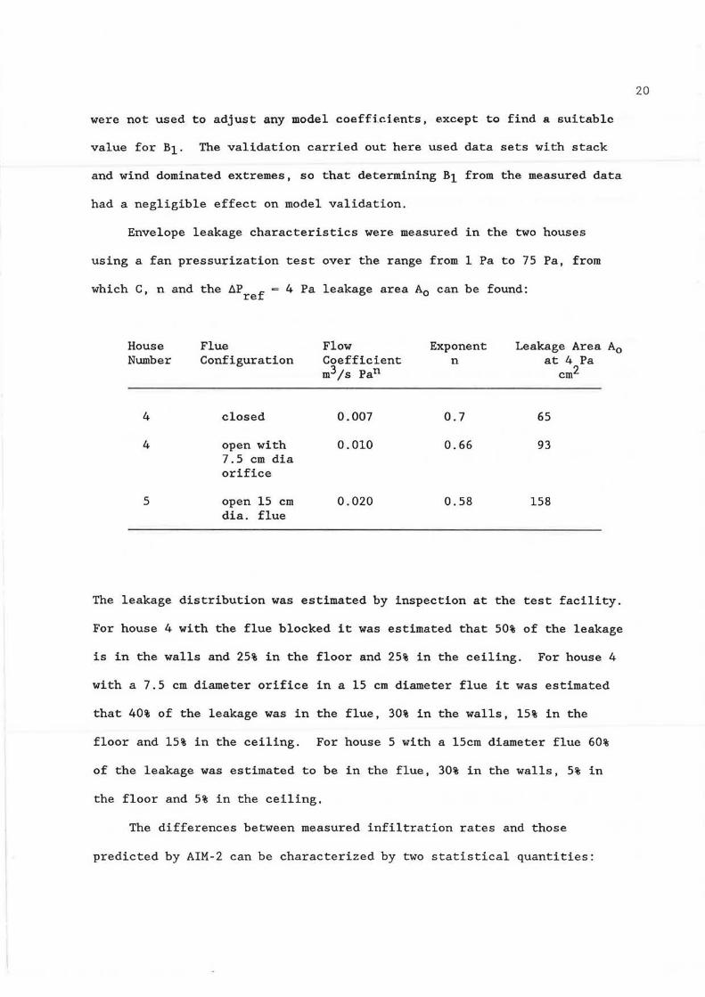
Envelope leakage characteristics were measured in the two houses
using a fan pressurization test over the range from 1 Pa to 75 Pa, from
which C, n and the AP f = 4 Pa leakage area A0 can be found: re
House Flue Flow Exponent Leakage Area A0 Number Configuration Coefficient n at 4 Pa
m3/s Pan cm2
4 closed 0.007 0.7 65
4 open with 0.010 0.66 93 7.5 cm dia orifice
5 open 15 cm 0.020 0.58 158 dia. flue
The leakage distribution was estimated by inspection at the test facility.
For house 4 with the flue blocked it was estimated that 50% of the leakage
is in the walls and 25% in the floor and 25% in the ceiling. For house 4
with a 7.5 cm diameter orifice in a 15 cm diameter flue it was estimated
that 40% of the leakage was in the flue, 30% in the walls, 15% in the
floor and 15% in the ceiling. For house 5 with a 15cm diameter flue 60%
of the leakage was estimated to be in the flue, 30% in the walls , 5% in
the floor and 5% in the ceiling.
The differences between measured infiltration rates and those
predicted by AIM-2 can be characterized by two statistical quantities:
20
bias and scatter. The bias can be thought of as the error in the
magnitude of the proportionality constants of the model equations, and the
scatter as the errors (and omissions of relevant variables) in the
functional form of the equation. The bias indicates the average error
that would be obtained over a long time period for all windspeeds and
temperature differences, and is found from the variation between the
calculated values and the mean measured value in each of the windspeed
ranges shown in Figures 5 through 8. The measured data was averaged in
bins 1 m/s wide. For each bin the mean is shown by a square symbol and
one standard deviation by error bars. The scatter indicates the error
that occurs for a single windspeed and temperature difference rather than
long time averaged mean values, and is found by subtracting the bias from
the calculated values and then averaging the absolute error for each
windspeed range bin. The other models included for comparison are:
• The LBL (USA) model (Sherman and Grimsrud (1980))
• The IRC/NRC (Canada) Variable n extension of the LBL model from
Yuill (1985) and Reardon (1989)
• The NRC (Canada) model of Shaw (1985)
• The BRE (U.K.) model of Warren and Webb (1980)
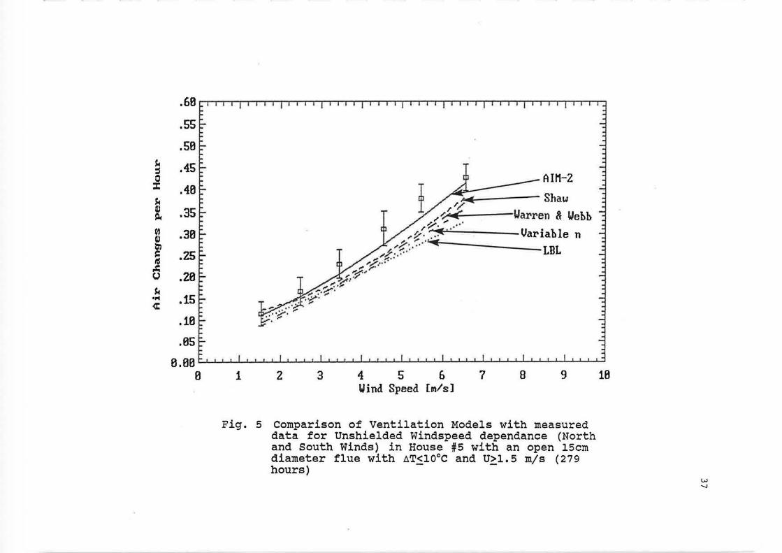
The predictions of AIM-2 and these four models, are compared to measured
data in Table 4 for unsheltered North and South wind direction conditions
in house 5 with a 15 cm diameter flue, and for house 4 with the flue
blocked. These results show that AIM-2 has the best overall performance
for houses with and without furnace flues because the furnace flue is
treated as a separate leakage site with its own wind pressure and wind
shelter coefficients. The same data used to calculate bias and scatter in
Table 2 are shown graphically in Figures 5 and 6.
21
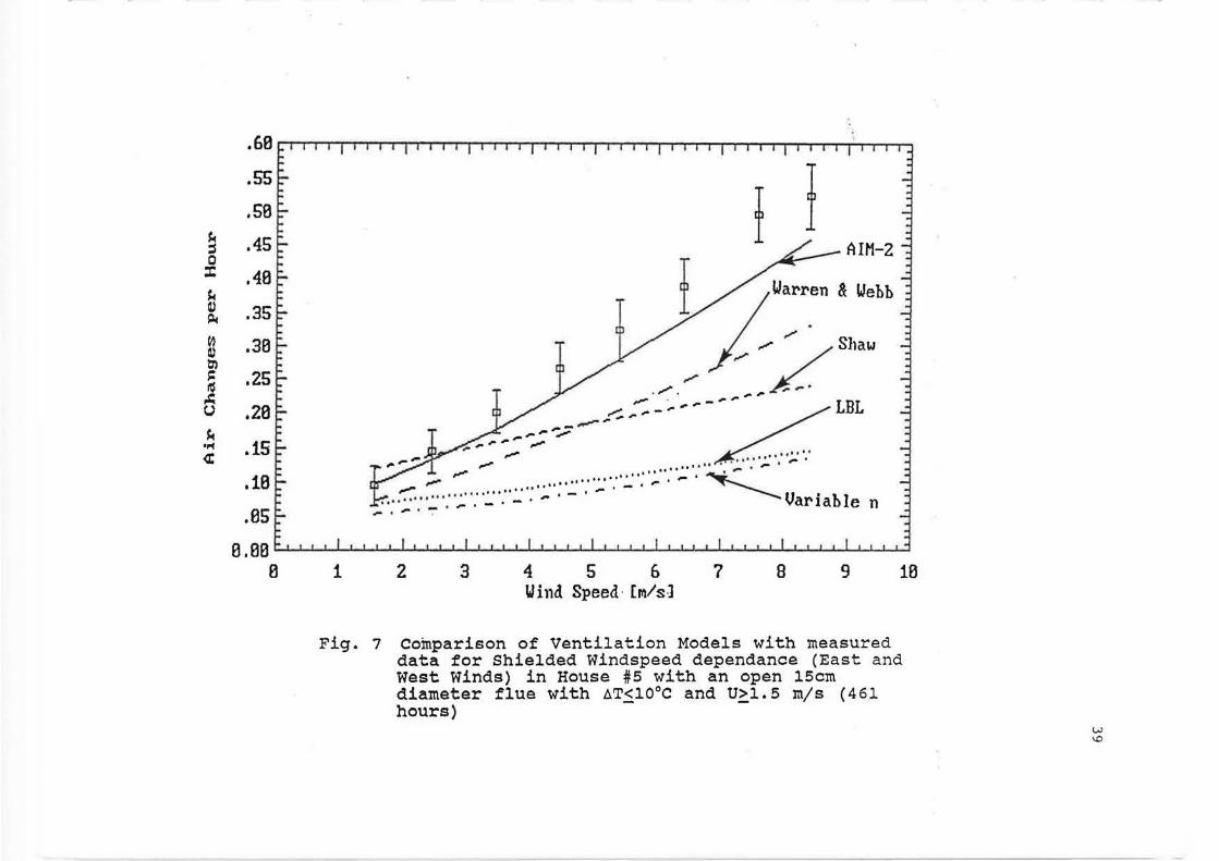
Figure 7 compares the windspeed dependence of the models for house 5
with an open 15 cm diameter flue where the house is heavily sheltered in
East and West winds. The shelter in this case is from the neighboring
houses in the row, where the gap between the houses is approximately three
metres (about one half of the house height). Warren and Webb's and Shaw's
models have relationships for sheltered or unsheltered buildings, but with
no variation in the degree of shelter. For these two models the sheltered
building relationships were used. The LBL and IRC/NRC variable n models
both use the same table of values for shelter that is originally from LBL,
and the shelter coefficient that most closely matches the shelter
condition for this case was chosen.
For AIM-2, Sw - 1.0 was used for unsheltered conditions, and "very
heavy shielding" Sw - 0.5 was used for the sheltered case, see Table 2. In
AIM-2 the shelter coefficient Sw appears directly as a windspeed
multiplier, and is the ratio of an effective sheltered windspeed,
U h lt d to the unsheltered windspeed, U h lt d' An equivalent s e ere uns e ere
value of Sw may be found for each model using (29).
s w
u [ l l/2n sheltered ~,sheltered uunsheltered ~.unsheltered
(29)
Substituting the appropriate equations for flowrate, with their different
shelter coefficients, and assuming a typical value of n - 2/3, values of
effective Sw for each model are summarized in Table 5, and range from 0.32
for the LBL model to a physically unrealistic value of 1.5 for Shaw's
model at a windspeed of 1 m/s.
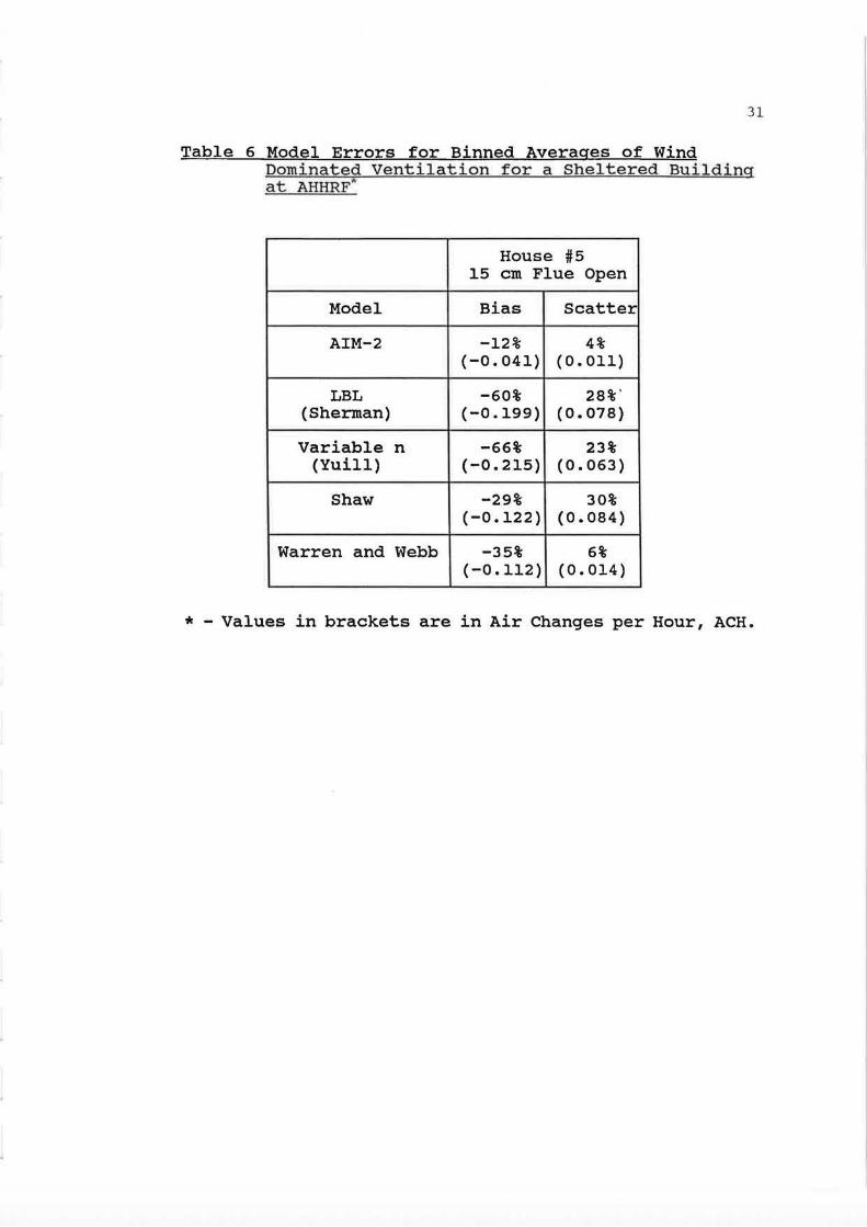
All the models except AIM-2 underpredict the wind effect infiltration
rate Qw significantly because they cannot have unshielded flue leakage
22

with a shielded building. A swnmary of the bias and scatter for each
model is given in Table 6.
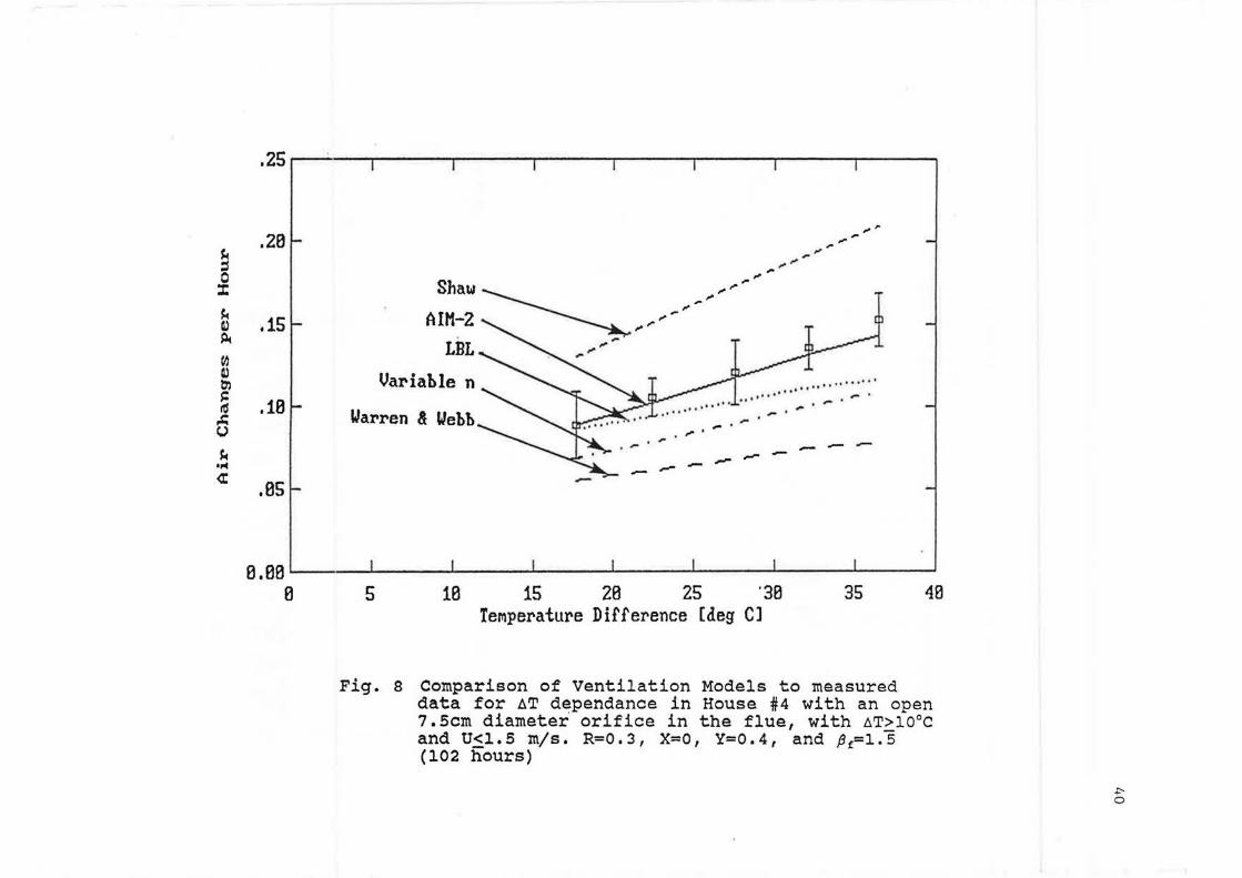
Figure 8 illustrates the temperature difference dependence of the
models for house 4 with a 7 . 5 cm diameter restriction orifice in the flue.
A sununary of the bias and scatter for each model is given in Table 7. As
before, AIM-2 gives the best overall agreement, because it allows the flue
leakage to be above the ceiling height for stack effect.
In almost all cases the LBL model has the greatest scatter. This is
because its assumption of orifice flow for the building envelope produces
an incorrect variation in ventilation rate with windspeed and temperature
difference .
Another significant source of error, common to all ventilation
models, lies in trying to predict ventilation rates based on weather data
measured at a site remote from the building under study. This is a common
practice since most meteorological data that is generally available is
measured at airports in flat unobstructed terrain. The wind speed must be
corrected for differences between the measurement site and the building
due to changes in terrain and localized shelter effects. The procedure
used in AIM-2 uses simple methods to correct the windspeed to account for
local shelter and differences between typical rural and urban terrain and
makes no attempt to correct the wind direction which may be altered by
both natural and man made structures (river valleys, hills, high rise
towers, etc.). For the test results presented here, all the
meteorological data was measured on site and these difficulties were not
encountered.
23

Effect of Changing Leakage Distribution on Model Predictions
To test the effect of leakage distribution, four different values for
the parameters R and X were chosen with Y (the fraction of leakage in the
flue) and Pf (the nondimensional flue height) unchanged. The resulting
model predictions were compared to data where stack effect dominates,
taken in house 4 with a 7.5 cm diameter orifice in the flue. The sum of
ceiling and floor leakage R was varied from zero to 0.4, and X (the
difference between ceiling and floor leakage) was varied from -0.l to
+0.2. The fraction of flue leakage, Y, was constant at 0.4, and the
nondimensional flue height, Pf, was 1.5. Shaw's and Warren and Webb's
models do not have leakage distribution parameters, and their predictions
do not change for these different cases.
The models compared in this section are AIM-2, LBL and the Variable n
model. The case of R-0.3, and X-0 is used as a basis for comparison. The
results show that the scatter is not significantly changed by the leakage
distribution parameters, as one would expect, because R, X, Y and Pt do
not change the functional forms of the equations predicting the flowrates.
Instead, these parameters change the lead constants, the stack and wind
factors, fs and fw, and will affect only the bias.
• For R - 0.2 and X - -0.1, the models increase their predicted values
by less than 8%, so that AIM-2 now overpredicts by 5.1% rather than
underpredicting by 3. 4%, and the underpredictions of t.hP. T.RT. ann
Variable n models are less by a similar amount.
• For R - 0 and X - 0, with all the non-flue leakage in the walls (not
a typical leakage distribution), the model predictions are changed by
less than 6%, a relatively small amount with AIM-2 underpredicting
less, and LBL and the Variable n model underpredicting more.
24
• The third distribution uses R - 0.4 and X - +0.2. Unlike putting all
the leakage in the walls this does not seem an unlikely leakage
distribution, yet it yields predictions reduced by about 20% for all
three models.
These tests show that correctly estimating leakage distribution can be an
important factor in predicting ventilation rates. However, it also shows
that it is possible for an atypical leakage distribution to produce
reasonable results.
Conclusions
• Including the furnace flue as a separate leakage site allows AIM-2 to
account for the effect of the flue on natural ventilation rates much
better than the other models tested here.
• Using a power law pressure-flow relationship for the building
envelope ensures that AIM-2 has the correct variation with changes in
windspeed and indoor-outdoor temperature differences.
• Model predictions are highly dependent on estimates of wind shelter
that can be difficult to quantify. Table 2 shows that different
estimates of this factor can vary the predicted ventilation rate by a
factor of two.
• Models that use leakage distribution parameters R, X and Y are
sensitive to the choice of these parameters. Typical variability in
estimating these parameters can change the predicted infiltration
rates by up to 20%.
Finally, the use of on-site meteorological towers removed the need for
transferring wind data from an airport location to the site. The uncer
tainty associated with the process should be examined in future studies.
25
References
A.I.V.C. (1986) "Air Infiltration Calculation Techniques - An Applications Guide" Air Infiltration and Ventilation Centre, Bracknell, U.K.
ASHRAE (1989) "Air Flow Around Buildings", Chapter 14 Handbook of Fundamentals.
Akins, R.E., Peterka, J.A. and Cermak, J.E . (1979) "Averaged Pressure Coefficients for Rectangular Buildings", Wind Engineering Vol. 1, Proc. 5th Int. Conf. pp. 369-380.
Hayson, J.C. and Swinton, M.C. (1987) "The Influence of Termination Configuration on the Flow Performance of Flues", Canada Mortgage and Housing Research Report.
Irwin, J.S. (1979) "A Theoretical Variation of the Wind Profile Power Law Exponent as a Function of Surface Roughness and Stability", Atmospheric Environment 13, pp. 191-194.
Reardon, J.T. (1989) "Air Infiltration Modelling Study", Report #CR5446.3, Energy Mines and Resources Canada, National Research Council of Canada.
Shaw, C.Y. (1985) "Methods for Estimating Air Change Rates and Sizing Mechanical Ventilation Systems for Houses", Building Research Note 237, Division of Building Research, National Research Council of Canada.
Sherman, M.H. and Grimsrud, D.T. (1980) "Measurement of Infiltration Using Fan Pressurization and Weather Data", Lawrence Berkeley Laboratory, Report #LBL-10852.
Warren, P.R., and Webb, B.C. (1980) "The Relationship Between Tracer Gas and Pressurization Techniques in Dwellings", Proc. First Air Infiltration Center Conference , pp. 245-276.
Wilson, D.J., and Dale, J.D., (1985) "Measurement of Wind Shelter Effects on Air Infiltration", Proceedings of Conference on Thermal Performance of the Exterior Envelopes of Buildings, Clearwater Beach, Florida, Dec. 2-5. 1985.
, Wiren, B.G. (1984) "Wind Pressure Distributions and Ventilation Losses for a Single-Family House as Influenced by Surrounding Buildings - A Wind Tunnel Study", Proc. Air Infiltration Centre Wind Pressure Workshop, Brussels, 1984.
Yuill, G.K. (1985) "Investigation of Sources of Error and Their Effects on the Accuracy of the Minimum Natural Infiltration Procedure", Report for Saskatchewan Research Council.
26
List of Figures
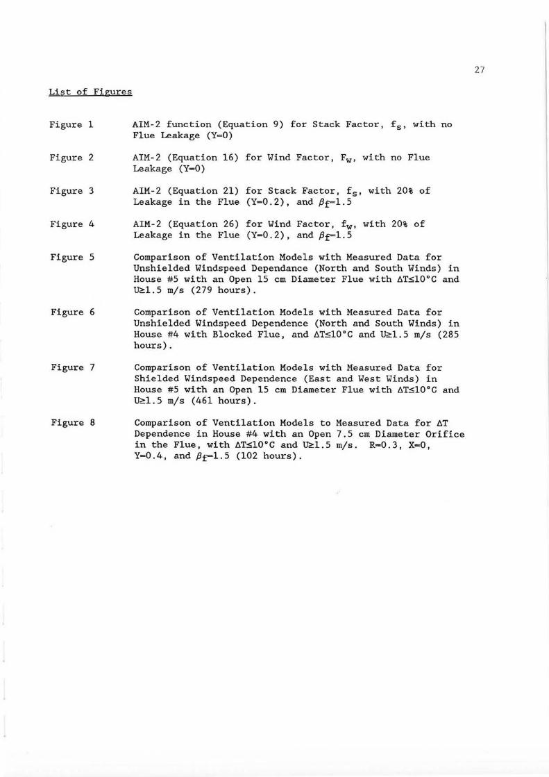
Figure 1
Figure 2
Figure 3
Figure 4
Figure 5
Figure 6
Figure 7
Figure 8
AIM-2 function (Equation 9) for Stack Factor, fs, with no Flue Leakage (Y=O)
AIM-2 (Equation 16) for Wind Factor, Fw, with no Flue Leakage (Y=O)
AIM-2 (Equation 21) for Stack Factor, fs, with 20% of Leakage in the Flue (Y=0 . 2), and Pp=l.5
AIM-2 (Equation 26) for Wind Factor, fw, with 20% of Leakage in the Flue (Y=0.2), and Pf=l.5
Comparison of Ventilation Models with Measured Data for Unshielded Windspeed Dependance (North and South Winds) in House #5 with an Open 15 cm Diameter Flue with AT~l0°C and U~l.5 m/s (279 hours).
Comparison of Ventilation Models with Measured Data for Unshielded Windspeed Dependence (North and South Winds) in House #4 with Blocked Flue, and AT~l0°C and U~l.5 m/s (285 hours).
Comparison of Ventilation Models with Measured Data for Shielded Windspeed Dependence (East and West Winds) in House #5 with an Open 15 cm Diameter Flue with AT~l0°C and U~l . 5 m/s (461 hours).
Comparison of Ventilation Models to Measured Data for AT Dependence in House #4 with an Open 7.5 cm Diameter Orifice in the Flue, with AT~l0°C and ~1.5 m/s. R- 0.3, X=O, Y-0.4, and Pf""'l.5 (102 hours).
27

Table 3 Construction Details of Houses Tested at AHHRF
House #4
Floor Area: 6250 x 6860 mm
Wall Height: 2440 mm
Basement Height: 2440 mm, 1830 mm Below Grade
Walls: 9.5 mm Prestained Rough Tex Plywood 50 mm Rigid Insulation
28
50 mm x 100 mm studs with fiberglass batt insulation 0.228 mm polyethylene Vapour Barrier
Windows:
13 mm Painted Gypsum Wallboard
North South : East West
None 2 - 2870 x 910 mm double glazed sealed 1090 x 1065 mm double glazed opening None
Ceiling: 9.5 mm plywood sheathing 0.228 mm polyethylene Vapour Barrier 13 mm Gypsum Wallboard
Door: 910 x 2030 mm insulated metal
House #5
Floor Area: 6250 x 6860 mm
Wall Height: 2440 mm
Basement Height: 2440 mm, 1830 mm Below Grade
Walls: 9.5 mm Prestained Rough Tex Plywood 50 mm x 100 mm studs with fiberglass batt insulation 0.152 mm polyethylene Vapour Barrier 13 mm Painted Gypsum Wallboard
Windows: North south East West
990 x 1950 mm double qlazed sealed None 1000 x 1950 mm double glazed opening 1000 x i950 mm double glazed opening
Ceiling: 9.5 mm plywood sheathing 0.152 mm polyethylene Vapour Barrier 13 mm Gypsum Wallboard
Door: 910 x 2030 mm insulated metal
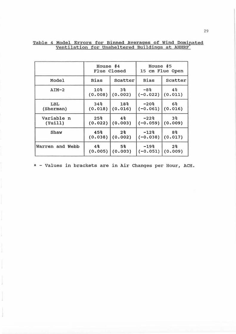
Table 4 Model Errors for Binned Averages of Wind Dominated Ventilation for Unsheltered Buildings at AHHRF*
House #4 House #5 Flue Closed 15 cm Flue Open
Model Bias Scatter Bias Scatter
AIM-2 10% 3% -8% 4% (0.008) (0.002) (-0.022) (0.011)
LBL 34% 18% -20% 6% (Sherman) (0.018) (0.016) (-0.061) (0.016)
Variable n 25% 4% -22% 3% (Yuill) (0.022) (0.003) (-0.059) (0.009)
Shaw 45% 2% -12% 8% (0.038) (0.002) (-0.038) (0.017)
Warren and Webb 4% 5% -19% 2% (0.005) (0.003) (-0.051) (0.009)
* - Values in brackets are in Air Changes per Hour, ACH.
29
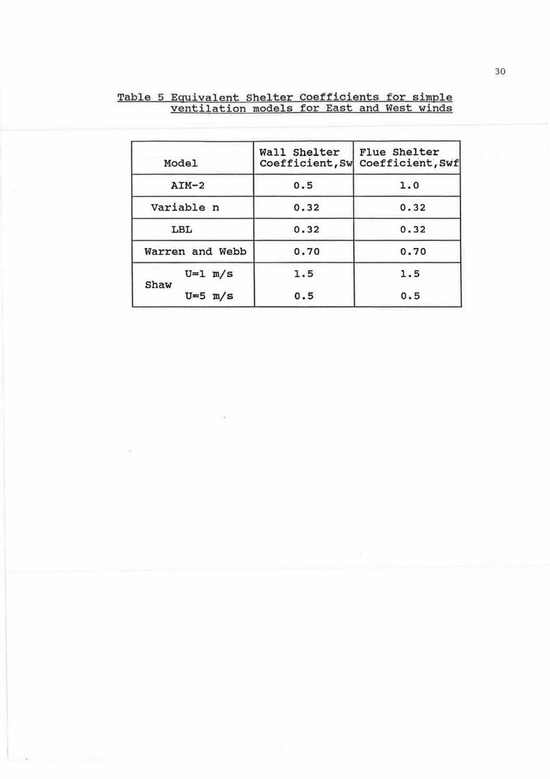
Table 5 Equivalent Shelter Coefficients for simple ventilation models for East and West winds
Wall Shelter Flue Shelter Model Coefficient,sw coefficient,Swf
AIM-2 0.5 1.0
Variable n 0.32 0.32
LBL 0.32 0.32
Warren and Webb 0.70 0.70
U=l m/s 1.5 1.5 Shaw
U=S m/s 0.5 0.5
30
31
Table 6 Model Errors for Binned Averages of Wind Dominated Ventilation for a Sheltered Building at AHHRF*
House #5 15 cm Flue Open
Model Bias Scatter
AIM-2 -12% 4% (-0.041) (0.011)
LBL -60% 28%' (Sherman) (-0.199) (0.078)
Variable n -66% 23% (Yuill) (-0.215) (0.063)
Shaw -29% 30% (-0.122) (0.084)
Warren and Webb -35% 6% (-0.112) (0.014)
* - Values in brackets are in Air Changes per Hour, ACH.
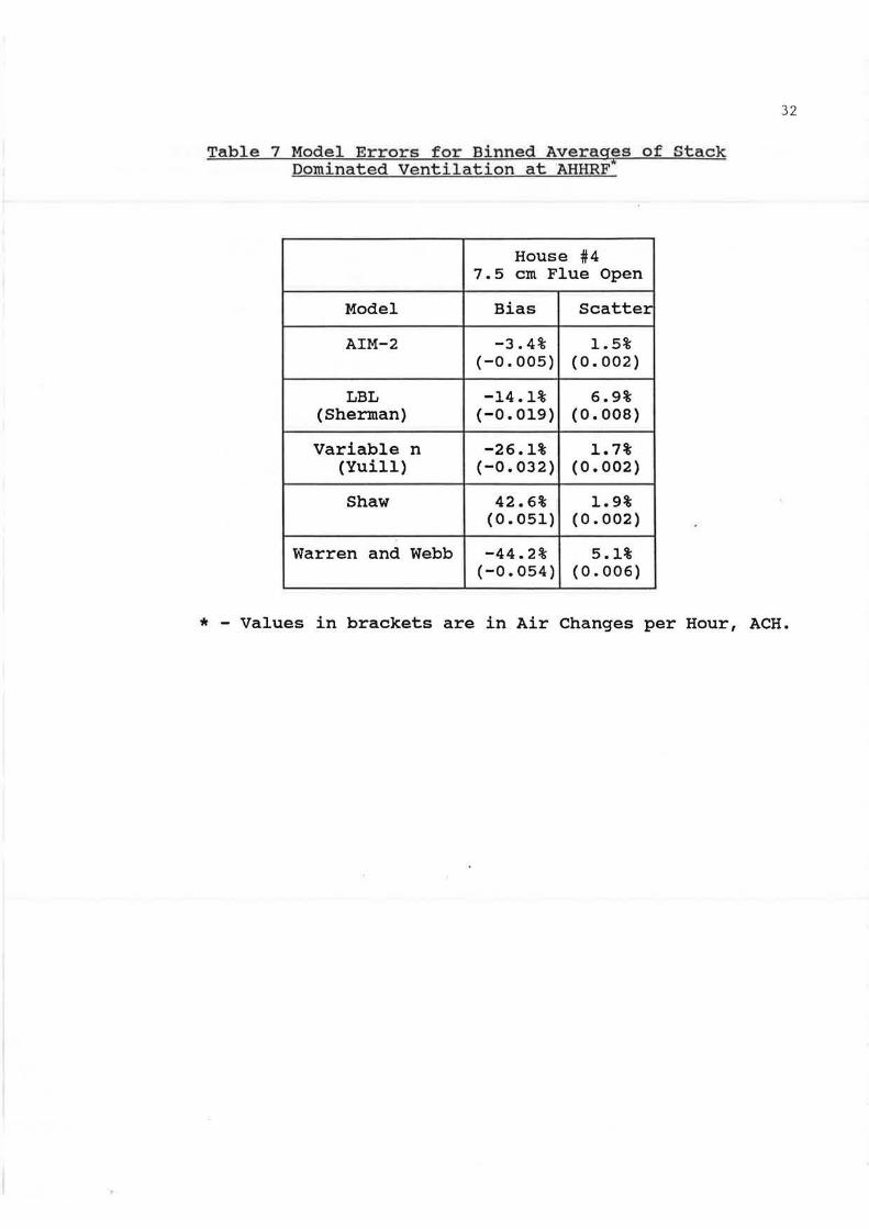
Table 7 Model Errors for Binned Averages of Stack Dominated Ventilation at AHHRF'
House #4 7.5 cm Flue Open
Model Bias Scatter
AIM-2 -3.4% 1.5% (-0.005) (0.002)
LBL -14.1% 6.9% (Sherman) (-0.019) (0.008)
Variable n -26.1% 1.7% (Yuill) (-0.032) (0.002)
Shaw 42.6% 1.9% (0.051) (0.002)
Warren and Webb -44.2% 5.1% (-0.054) (0.006)
32
* - Values in brackets are in Air Changes per Hour, ACH.
Cl) c.. .. s... 0 ~ (.) ~ ~
.:.: (.) ~
t;
.50r---r---r---r-----r~.--.....--.--..----,.~.---.---.---.--...~.-------.---.---.
.40
~ R = 1 .30
I / R = .5
.2~~ /" R = 0 +
.10
0.00~..l..--1---1-----L~.l..-...l.---1.-_.J...__J,~j___.__J_--1...--1.~.1.--..l_--1.-_J_----1.~
-1.0 -.8
Figure 1
-.6 -.4 -.z -.0 .z .4 .6 .8 1.0 X, Vertical Leakage Distribution
AIM-2 function (Equation 9) for Stack Factor, f 5 ,
with no Flue Leakage (Y=O)
w w
3 c..
"I
~ 0 ~ 0
~ "d $:
•1'4
3
.300 ,-....--r----..-----r-..-....--r---.--~----r----ir-....--.---.--~----r-ir-....--.--....
.200 R = .4
.150 ·-
.100 ·-
.050·-
0. 000 ,_...._......._.........___.___..__..._1....--......._-L---'---L--.l...---l.___JL.__.1..-...l.--'--_.,l_-L~ -L0 -.a
Figure 2
-.6 -.4 -.z -.0 .2 .4 .G .8 1.0 X, Vertical Leakage Distribution
AIM-2 (Equation 16) for Wind Factor, Fw, with no Flue Leakage (Y=O)
w +=-
l! .... ~
1) ~ 'E ~
t,;
.s0 r-r--r---,----.---r--r--r-.--y---i~---.---.---.--.---,--........--
.40
.30
.20
.10L ~R=.8
0.00.___,__.__.___._~.____.___,___,___.___._~.___.___,___,___.___._~.__.....__.__,
-1.0 -.8
Figure 3
-.6 -.4 -.2 -.0 .2 .4 .6 .8 1.0 X, Vertical Leakage Distribution
AIM-2 (Equation 21) for Stack Factor, fs, with 20% of Leakage in the Flue (Y=0.2), and fit=l.S
w V1
3
'" " M 0 il (J Id ~
'd s: •..C
3
.300r---r---r-.--r--r--r---r~.-.--r-.---.-r~--.--,~.-r--r--i
.250
.200
.150
.1001
.050
0.0001 '--"-_.._--1...----1-.1.---!--"--l..--J-.L.-_.1._--.L.---L__Jl.....-..r._--1---.L...-1._i___j
-1.0 -.8
FiJgure 4
-.6 -.4 -.z -.0 .2 .4 .6 .8 1.0 X, Vertical Leakage Distribution
AIM-2 (Equation 26) for Wind Factor, fw, with 20% of Leakage in the Flue (Y=0.2), and fif=l.5
w °'
.60
.55
.50 S-4 .45 ::$ 0 ::c .40 S-4 4) .35 ~
"' .30 4) ~ j: .ZS It! .:: () .20 Sc
•1'4 .15 ~
.10
.05
0.00 0 1
AIM-2
l'J/~ SJ1aw /,,,,.; II ,p, ',,. .·. . warren & Uebb
/'.I' ... -.c I' ,,.y. .. II • b ,,,/'· "." .. · ._.... var 1a le n . ~ ,,., .· ,,/~. :·· · LBL
,,."'~·" ' ~,
;:f.··,... ,,. ": ·:ii
:;.~·~· .. y.
:;-:.,· I o o ,:..•r .,,. " ·?· ,,
2 3 4 5 6 7 8 9 Wind Speed [~Isl
Fig. 5 Comparison of Ventilation Models with measured data for Unshielded Windspeed dependance (North and South Winds) in House #5 with an open 15cm diameter flue with ~T~l0°C and U~l.5 m/s (279 hours)
10
VJ -....)

S.. :$ 0 ::t
a . ~
"' 0 ~
~ ~ 0
t.c •..C
<C
.251 I I I I I Ii Ii I I 1 I I I Ill It I i Ii I I J l I I I Ii I i I J I I I i I ti I Jr I 1 1
.20
.15
.10
.05
/ I
/ /
/' I
/'
I
, /
/""! SJ1aw
/ 'T' • /' .h1 A IM-2 / 1/
/
r /' .v~
/'/'/';~~+ I LBL / .. ··
/' ~· , ... · ~.·~-, ,.,,, t:• • r
.-;·/',.. ·~· v ···~··;,.." ... ··;,,- / /"
··~~ ~ 7 ,,. ~~· ''l
0 . 00 L-.L- I I I I I I I I I ' I I I I , I I I I , ' I I I I I I I I I I I I I ' I , ' ' I I I I I I ' I I
0 1 2 3 4 5 6 7 8 9 10 Uind Speed [~Isl
Fig. 6 Comparison of Ventilation Models with measured data for Unshielded Windspeed dependance (North and South Winds)in House #4 with blocked flue, and ~T<l0°C and U~l.5 m/s (285 hours)
w ro
.60
.55
.50 M .45 ::s 0
:c .40 M ~ .35 Poe
"' .30 ~ ~ s: .ZS It! ~ (.) .Z0 M
. 15 ·~ ~
.10
. 05
0.00 0 1
! 1 AIM-2
Warren & lJebb
// · S!1aw
" /. ~ . .. ,. - ,.
. ~ . _L,.,.,.,. LBL ~,..,,. _,.,.
- .... ,. .. . ,. ,. ,,,, .. .. .. . ,. ,. . .. ,. ,. ,.,.,. .. .. . ,,,,,,,. t. t I I
~ ,,..,,..,,.. ,.,.,. ...... ·~· ·. - . _, ········:.:·: - · - Variable n ,,,,. ,,11•t••'', - I.,....
,,,,. I I • I I I ' I I I I - I ,,.
I 1' I f 11 I·:.: I I ,. I -- . . -'
2 3 4 5 6 7 8 9 Uind Speed · [l'l\ls.]
10
Fig. 7 Comparison of Ventilation Models with measured data for Shielded Windspeed dependance (East and west Winds) in House #5 with an open 15cm diameter flue with ~T~10°C and U~l.5 m/s (461 hours)
w ID
M :;$ 0 :t: M G,) ~
'1 G,) ~ $:: ~ ~ u ~
'" <C
.251---r---r--i----r---r--.----r------..
,. ,. ,, ,. ,. ,. ,. .201
.15 I I.RT. - ~ ,.. ,..
········ · · · ·~·:· Variable n .. . . . . .. . ,.. . ,,. -. 10 Uarren & Webb
- - -- -.05 -
0.00l....--·~-'-~~....J-~~-1-~~-L~~-L~~_L~~_J_~~__J
0 5 10 15 20 25 '30 35 40 TeMperature Ditference [deg CJ
Fig. 8 Comparison of Ventilation Models to measured data for AT dependance in House #4 with an open 7.Scm diameter orifice in the flue, with AT>l0°C and U<l.5 m/s. R=0.3, X=O, Y=0.4, and fif=l.5 (102 hours)
+:-0