The Aggregate Implications of

Regional Business Cycles*

Martin Beraja Erik Hurst Juan OspinaUniversity of Chicago

March 15, 2016

Abstract

We argue that it is difficult to make inferences about the drivers of aggregate business cyclesusing regional variation alone because (i) the local and aggregate elasticities to the same type ofshock are quantitatively different and (ii) purely aggregate shocks are differenced out when usingcross-region variation. We highlight the importance of these issues in a monetary union model,and by contrasting the behavior of US aggregate time-series and cross-state patterns during theGreat Recession. In particular, using household and retail scanner data for the US, we documenta strong relationship across states between local employment growth and local nominal and realwage growth. These relationships are much weaker in US aggregates. In order to identify theshocks driving aggregate (and regional) business cycles we develop a methodology that combinesregional and aggregate data. The methodology uses theoretical restrictions implied by a wagesetting equation that holds in many monetary union models with nominal wage stickiness. Weshow how to estimate this equation using cross-state variation—thus linking particular regionalpatterns to particular aggregate shock decompositions. Applying the methodology to the US,we find that a combination of both "demand" and "supply" shocks are necessary to account forthe joint dynamics of aggregate prices, wages and employment during the 2007-2012 periodwhile only "demand" shocks are necessary to explain most of the observed cross-state variation.We conclude that the wage stickiness necessary for demand shocks to be the primary cause ofaggregate employment decline during the Great Recession is inconsistent with the flexibility ofwages estimated from cross-state variation.

*First draft: May 2014. A previous version of this paper circulated as "The Regional Evolution of Prices and WagesDuring the Great Recession". We thank Mark Aguiar, Manuel Amador, David Argente, Mark Bils, Juliette Caminade,Elisa Giannone, Adam Guren, Simon Gilchrist, Paul Gomme, Bob Hall, Marc Hofstetter, Loukas Karabarbounis, PatKehoe, Virgiliu Midrigan, Elena Pastorino, Harald Uhlig, Joe Vavra and Ivan Werning for their very helpful commentsand suggestions. Finally, we thank seminar participants at the Bank of England, Berkeley, the Board of Governors of theFederal Reserve, Boston University, Brown, Chicago, Chicago Federal Reserve, Columbia, Duke, Harvard, IEF Workshop,Michigan, Minneapolis Federal Reserve, Minnesota Workshop in Macroeconomic Theory, MIT, NBER’s Summer InstituteEF&G, NBER’s Summer Institute Prices Program, Northwestern, Princeton, Rochester, St. Louis Federal Reserve, UCLA,Yale’s Cowles Conference on Macroeconomics. Any remaining errors are our own. E-mail: martinberaja@gmail.com,erik.hurst@chicagobooth.edu, and juan.jose.ospina@gmail.com.

1 Introduction

A large and growing literature is exploiting regional variation to learn about the determinants ofaggregate economic variables.1 However, we argue that making inferences about the aggregate econ-omy using only regional variation is complicated by two issues. First, we show that, in a monetaryunion model, local and aggregate elasticities to the same type of shock are quantitatively differentboth because of factor mobility and general equilibrium forces. This discrepancy makes it problem-atic to use local shock elasticities estimated from regional data to ascertain the importance of a givenaggregate shock. Second, purely aggregate shocks get differenced out when using cross-region vari-ation. As a result, it is not possible to learn anything about these aggregate shocks by exploitingvariation across regions. Furthermore, we provide evidence of both these issues by contrasting thebehavior of US aggregate time-series and cross-state patterns during the Great Recession. We docu-ment a strong relationship across states between local employment growth, and local nominal andreal wage growth. These relationships are much weaker in US aggregates. In summary, we cannotexpect to understand the joint evolution of aggregate variables by using cross-regional variationalone.

Therefore, we present a methodology that uses regional data along with aggregate data in orderto identify aggregate shocks driving business cycles. The methodology exploits theoretical restric-tions implied by a wage setting equation that hold in many monetary union models with wagestickiness. In turn, the extent to which aggregate wages are sticky is a key restriction in identifyingthe type of shocks driving aggregate fluctuations (e.g., "demand" vis a vis "supply" shocks)2. Undercertain conditions, we show how to use cross-region variation in wages, prices, and employmentto estimate this wage setting equation—thus parameterizing the theoretical restrictions and linkingregional business cycles to shock decompositions of aggregate business cycles.

Using household and retail scanner data for the US, we construct state-level wage and priceindices as well as a measure of employment. Given the strong comovement of wages and employ-ment across states, our estimates of the wage setting equation suggest that wages are relativelyflexible—thus limiting the contribution of "demand" shocks to aggregate employment decline dur-ing the Great Recession. Instead, we find that a combination of "demand" and other shocks arenecessary to account for the joint dynamics of aggregate prices, wages and employment during the2007–2012 period. In particular, the relative stability of aggregate wages in the time-series comparedto state-level wages is not caused by wage stickiness, but because different aggregate shocks haverelatively offsetting effects on aggregate wages. We conclude that the wage stickiness necessaryfor demand shocks to be the primary cause of aggregate employment decline during the GreatRecession is inconsistent with the flexibility of wages estimated from cross-state variation.

1For recent examples, see Autor et al (2013), Charles et al (2015), Hagedorn et al (2015), Mehrotra and Sergeyev (2015),Mian and Sufi (2014) and Mondragon (2015).

2We refer to a "demand" shock as a shock that moves employment and real wages in opposite directions and movesemployment and prices in the same direction. In the model of the monetary union we develop below, these shocks canbe formalized as shocks to the household’s discount rate or as shocks to the aggregate nominal interest rate rule. Ourmodel also allows for a productivity/markup shock and a shock to household preference for leisure.

1

The paper is organized as follows. In Sections 2 and 3, we begin by documenting a series of newfacts about the variation in nominal and real wages across US states during the Great Recession.Using data from the 2000 US Census and the 2000 - 2012 American Community Surveys (ACS), weconstruct state-level nominal wage indices during the 2000 to 2012 period. We restrict our sampleto full time workers with a strong attachment to the labor force. We adjust our wage measuresto cleanse them from observable changes in labor force composition over the business cycle. Inorder to construct a measure of real wages we deflate our nominal wage indices with state-levelprice indices created using data from Nielsen’s Retail Scanner Database. The Retail Scanner Databaseincludes weekly prices and quantities for given UPC codes at over 40,000 stores from 2006 through2012. While the price indices we create from this data are based mostly on consumer packagedgoods, we show how under certain assumptions the indices can be scaled to be representative of acomposite local consumption good. Furthermore, we show that an aggregate price index createdwith the retail scanner data matches the BLS’s Food CPI nearly identically.

Using our indices, we show that states that experienced larger employment declines between2007 and 2010 had significantly lower nominal and real wage growth during the same time period.These cross-state patterns stand in sharp contrast with the well documented aggregate time-seriestrends for prices and wages during the same time period. As both aggregate output and employ-ment contracted sharply in the US during the 2007-2012 period, aggregate nominal wage growthremained robust and real wage growth did not break trend.3 In sum, while aggregate wages appearto be sticky during the Great Recession, state-level wages do not.

In Section 4, we present a monetary union model that we use for two purposes. First, a calibratedversion of the model allows us to sign the elasticities to a given shock and quantify the differencesbetween aggregate and local elasticities. Second, the model makes explicit assumptions that are suf-ficient to estimate the parameters in an aggregate wage setting equation using cross-state variationin employment, wages and prices. As we highlight below, these parameters help us identify theunderlying aggregate drivers of the joint dynamics of employment, wages and prices.

The model has many islands linked by trade in intermediate goods which are used in the pro-duction of a non-tradable final consumption good. The only asset is the economy is a one-period,non-state contingent nominal bond. The nominal interest rate on this asset follows a rule that en-dogenously responds to aggregate variables and is set at the union level. Labor is the only otherinput in production, which is not mobile across islands. We assume that nominal wages are onlypartially flexible. This is the only nominal rigidity in the model. Finally, the model includes multipleshocks: a shock to the household’s discount rate, shocks to non-tradable and tradable productiv-ity/markup, a shock to the household’s preference for leisure, and a monetary policy shock. Asidefrom the monetary policy shock, all shocks have both local and aggregate components. By defi-nition the weighted average of the local shocks sum to zero. We show that, under relatively fewassumptions, the log-linearized economy aggregates. This allows us to study the aggregate and lo-

3The robust growth in nominal wages during the recession is viewed as a puzzle for those that believe that the lackof aggregate demand was the primary cause of the Great Recession. For example, this point was made by Krugman in arecent New York Times article ("Wages, Yellen and Intellectual Honesty", NYTimes 8/25/14).

2

cal behavior separately, a property that we will exploit when estimating the aggregate and regionalshocks through our methodology.

Using a calibrated version of the model, we show that local employment elasticities to a localdiscount rate shock are two to three times larger than the aggregate employment elasticity to a simi-larly sized aggregate discount rate shock. This implies that elasticities often estimated for "demand"shocks (i.e., our discount rate shock) using cross-region variation are likely to dramatically overstatethe elasticities of aggregate variables to "demand" shocks in the aggregate. The key general equi-librium forces in the model that may dampen aggregate elasticities are the endogenous response ofnominal interest rates to aggregate variables and trade in the intermediate input. We show that localand aggregate elasticities get much closer together when the interest rate does not endogenouslyrespond to changes in aggregate prices or employment (as when the economy is close to the zerolower bound).4

In Section 5, we turn to estimation of aggregate shocks. We present a procedure that allow usestimate the shocks in a larger class of monetary union models than the benchmark model outlinedabove, thus imposing less a-priori structure and making the analysis more persuasive. In particular,we consider models where the aggregate and local equilibria can be represented as a structuralvector autoregression (SVAR) in price inflation, nominal wage inflation, and employment with threeshocks. We refer to the three shocks as the discount rate shock (which is a combination of thediscount rate and monetary policy shock), the productivity/markup shock (which is a combinationof the productivity/markup shocks in the tradable and non tradable sectors) and the leisure shock(which is the shock to leisure preference). In order to identify the aggregate shocks, we estimatea SVAR and impose certain properties of our benchmark monetary union model. Our results willbe consistent with monetary union models that satisfy all of these. First, we use the aggregatewage setting equation to derive a series of linear restrictions linking the reduced form errors to theunderlying structural shocks. Second, we use the sign of the joint-response of employment, wagesand prices (on impact) to a discount rate and a productivity/markup shock.5 These two, togetherwith the usual shock-orthogonality conditions, are sufficient to identify the structural shocks.

The methodology requires parameterizing the structural wage setting equation. We use state-level data on prices, wages and employment during the 2006-2012 period to estimate the two pa-rameters in our base specification, i.e., the Frisch elasticity of labor supply and the degree of wagestickiness. Across a variety of specifications and identification procedures, including instrumentingfor local labor demand shocks, we estimate only a modest degree of wage stickiness. These esti-mates are much smaller than estimates of wage stickiness obtained using only aggregate time-seriesdata.

4A similar point is made in Nakamura and Steinsson(2014) with respect to local estimates of fiscal multipliers.5We view this methodology as an additional contribution of our paper. Beraja (2015) presents an extension of this

scheme to a more general class of models. These are part of a growing literature developing “hybrid" methods that,for instance, constructs optimal combinations of econometric and theoretical models (Carriero and Giacomini (2011),Del Negro and Schorfheide (2004)) or uses the theoretical model to inform the econometric model’s parameter (Anand Schorfheide (2007), Schorfheide(2000)). Our procedure is closest in spirit to the procedure recently developed inBaumeister and Hamilton (2015).

3

With the parameterized aggregate wage setting equation, we use the SVAR identification pro-cedure described above to estimate the shocks driving aggregate employment, prices, and wagesduring the Great Recession. Our results suggest that during the early part of the recession (2008-2009) roughly 30 percent of the aggregate employment decline can be attributed to the discountrate shock (i.e., the "demand" shock). The leisure shock explains roughly 30 percent of the declinein aggregate employment while the productivity/markup shock explains the remaining 40 percent.Over a longer period (2008-2012), however, the discount rate shock cannot explain any of the persis-tence in employment decline. Instead, it is the productivity/markup and labor supply shocks thatexplain why employment remained low from 2010-2012. In sum, while "demand" shocks may havebeen important in the early part of the recession, they cannot explain the persistently low levelsof employment in the US after 2009.6 Furthermore, we find that the aggregate leisure shock - notsticky wages - explains why aggregate wages did not fall during the Great Recession.

Our paper contributes to many literatures. First, our work contributes to the recent surge inpapers that have exploited regional variation to highlight mechanisms of importance to aggregatefluctuations. For example, Mian and Sufi (2011 and 2014), Mian, Rao, and Sufi (2013) and Midriganand Philippon (2011) have exploited regional variation within the US to explore the extent to whichhousehold leverage has contributed to the Great Recession.7 Nakamura and Steinsson (2014) usesub-national US variation to inform the size of local government spending multipliers. Blanchardand Katz (1991), Autor et al. (2013), and Charles et al. (2015) use regional variation to measure theresponsiveness of labor markets to labor demand shocks. Our work contributes to this literature ontwo fronts. First, we show that local wages also respond to local changes in economic conditions atbusiness cycle frequencies. Second, we provide a procedure where local variation can be combinedwith aggregate data to learn about the nature and importance of certain mechanisms for aggregatefluctuations. With respect to the latter innovation, our paper is similar in spirit to Nakamura andSteinsson (2014).

Second, our paper contributes to the recent literature trying to determine the causes of theGreat Recession. In many respects, our model is more stylized than others in this literature in thatwe include a broad set of shocks without trying to uncover the underlying micro-foundations forthese shocks. However, the shocks we chose to focus on were designed to proxy for many of thepopular theories about the drivers of the Great Recession. For example, our discount rate shockcan be thought of as reduced form representation of tightening of household borrowing limits.For example, such shocks have been proposed by Eggertsson and Krugman (2012), Guerrieri andLorenzoni (2011) and Mian and Sufi (2014) as an explanation of the 2008 recession. Likewise, our

6Christiano et al (2015a) estimate a New Keynesian model using data from the recent recession. Although theirmodel and identification are different from ours, they also conclude that something akin to a supply shock is needed toexplain the joint aggregate dynamics of prices and employment during the Great Recession. Likewise, Vavra (2014) andBerger and Vavra (2015) document that prices were very flexible during the Great Recession. They also conclude thatsomething more than a demand shock is needed to explain aggregate employment dynamics given the missing aggregatedisinflation.

7There has been an explosion of papers using regional data to better understand aggregate dynamics during the GreatRecession. Some recent papers include: Giroud and Mueller (2015), Hagedorn et al. (2015), Mehrotra and Sergeyev(2015), and Mondragon (2015).

4

productivity/markup shock can be interpreted as anything that changes firms’ demand for labor.In a reduced form sense, credit supply shocks to firms, such as those proposed by Gilchrist et al(2014), would be similar to our productivity/markup shock. Finally, our leisure shock can be seenas a proxy for increased distortions in the labor market due to changes in government policy (e.g.,Mulligan (2012) or as a reduced form representation of a skill mismatch story within the labormarket (e.g., Charles et al. (2013, 2015)).

2 Creating State-Level Price And Wage Indices

2.1 State-Level Wage Index

To construct nominal wage indices at the state level, we use data from the 2000 Census and the 2001-2012 American Community Surveys (ACS). The 2000 Census includes 5 percent of the US populationwhile the 2001-2012 ACS’s includes around 600,000 respondents per year between 2001 and 2004and around 2 million respondents per year between 2005 and 2012. The large coverage allows us tocompute detailed labor market statistics at the state level. For each year of the Census/ACS data, wecalculate hourly nominal wages for prime-age males with a strong attachment to the labor force. Inparticular, we restrict our sample to only males between the ages of 21 and 55, who were employedat the time of the Census, who reported usually working at least 30 hours per week, and whoworked at least 48 weeks during the prior 12 months. Then, for each individual in the resultingsample, we divide total labor income earned during the prior 12 months by a measure of annualhours worked during prior 12 months.8

Despite our restriction to prime-age males with a strong attachment to the labor force, the com-position of workers on other dimensions may still differ across states and within a state over time.The changing composition of workers could be explaining some of the variation in nominal wagesacross states over time. To cleanse our wage indices from these compositional issues, we createa composition adjusted wage measure (at least based on observables) by running the followingregression on the ACS data:

ln(witk) = γt + ΓtXit + ηitk

where ln(wikt) is log nominal wages for household i in period t residing in state k and Xit is avector of household specific controls. The vector of controls include a series of dummy variablesfor usual hours worked (with "40-49 hours per week" being the omitted group), a series of five yearage dummies (with "40-44" being the omitted group), four educational attainment dummies (with"some college" being the omitted group), three citizenship dummies (with "native born" being theomitted group), and a series of race dummies (with "white" being the omitted group). We run theseregressions separately for each year so that both the constant, γt, and the vector of coefficients on

8Total labor income during the prior 12 months is the sum of both wage and salary earnings and business earnings.Total hours worked during the previous 12 month is the product of total weeks worked during the prior 12 months andthe respondents report of their usual hours worked per week.

5

the controls, Γt, can differ for each year. Then, we take the residuals from these regressions, ηitk,and add back the constant, γt. Adding back the constant from the regression preserves differencesover time in average log-wages. To compute average wages in a state holding composition fixed, weaverage eηitk+γt across all individuals in state k. We refer to this measure as the "adjusted nominalwage index" in time t in state k. This is the series we use to exploit cross-state variation in wagesduring the Great Recession.

The benefit of the Census/ACS data is that it is large enough to compute detailed labor marketstatistics at state levels. However, one drawback of the Census/ACS data is that it not available at anannual frequency prior to 2000. To complement our analysis, we use data from the March Supple-ment of the Current Population Survey (CPS) to examine longer run aggregate trends in both nominaland real wages. These longer run trends are an input into our aggregate shock decomposition pro-cedure discussed below. We compute the wage indices using the CPS data analogously to the waywe computed the wage indices within the Census/ACS data.9 For the remainder of the paper, weuse the Census/ACS data to explore regional wage variation and the CPS data to examine aggre-gate time series wage variation. However, for the 2000-2012 period, we can compare the time-seriesvariation in aggregate wages using the Census/ACS data with the time series variation in aggregatewages using the CPS data. The two series have a correlation of 0.99 during this time period.

2.2 State-Level Price Index

2.2.1 Price Data

State-level price indices are necessary to measure state-level real wages. In order to construct state-level price indices we use the Retail Scanner Database collected by AC Nielsen and made available atThe University of Chicago Booth School of Business.10 The Retail Scanner data consists of weeklypricing, volume, and store environment information generated by point-of-sale systems for about90 participating retail chains across all US markets between January 2006 and December 2012. As aresult, the database includes roughly 40,000 individual stores selling, for the most part, food, drugsand mass merchandise.

For each store, the database records the weekly quantities and the average transaction price forroughly 1.4 million distinct products. Each of these products is uniquely identified by a 12-digitnumber called Universal Product Code (UPC). To summarize, one entry in the database containsthe number of units sold of a given UPC and the weighted average price of the corresponding

9In particular, we compute hourly wages for men 21-55 with a strong attachment to the labor force (those currentlyworking at least 30 hours a week and those who worked at least 48 weeks during the prior year). Again, like for the ACSdata, we adjust the wages to account for a changing vector of observables over time. A full discussion of our methodologyto compute composition adjusted wages in the CPS can be found in the Online Appendix that accompanies the paper.

10The data is made available through the Marketing Data Center at the University of Chicago Booth School of Business.Information on availability and access to the data can be found at http://research.chicagobooth.edu/nielsen/. Con-temporaneously, Coibion et al. (2015), Kaplan and Menzio (2015) and Stroebel and Vavra (2014) also use local scannerdata/household price data to estimate that local prices vary with local economic conditions at business cycle frequencies.Our paper complements this literature by actually making price indices using the Nielsen scanner data for each state atthe monthly frequency and using those price indices to estimate structural parameters of the local wage setting equation.

6

transactions, at a given store during a given week. The database only includes items with strictlypositive sales in a store-week and excludes certain products such as random-weight meat, fruits,and vegetables since they do not have a UPC assigned. Nielsen sorts the different UPCs into overone thousand narrowly defined "categories". For example, sugar can be of 5 categories: sugargranulated, sugar powdered, sugar remaining, sugar brown, and sugar substitutes. We use thesecategories when defining our price indices.

Finally, the geographic coverage of the database is outstanding and is one of its most attractivefeatures. It includes stores from all states except for Alaska and Hawaii. Likewise, it covers storesfrom 361 Metropolitan Statistical Areas (MSA) and 2,500 counties. The data comes with both zipcode and FIPS codes for the store’s county, MSA, and state. Over the seven year period, the data setincludes total sales across all retail establishments worth over $1.5 trillion. In this paper, we aggre-gate data to the level of US states and compute state-level retail scanner data price indices. OnlineAppendix Table R1 shows summary statistics for the retail scanner data for each year between 2006and 2012 and for the sample as a whole.11

2.2.2 A Retail Scanner Data Price Index

In order to construct state-level price indices we follow the BLS construction of the CPI as closelyas possible.12 While we briefly outline the price index construction in this sub-section, the fulldetails of the procedure are discussed in the Online Appendix that accompanies our paper. Ourretail scanner price indices are built in two stages. In the first stage, we aggregate the prices ofgoods within the roughly 1,000 categories described above. For our base indices, a good is a givenstore-UPC pair such that a UPC in store A is treated as a different good than the same UPC sold instore B. This allows for the possibility that prices may change as households substitute from a highcost store (that provides a different shopping experience) to a low cost store when local economicconditions deteriorate. Then, we compute, for each good, the average price and total quantity soldin a given month and state. Next, we construct the quantity weighted average price for all goods ineach detailed category in a given month and state. We aggregate our index to the monthly level toreduce the number of missing values.13

Specifically, for each category, we compute:

11The Online Appendix is available at http://faculty.chicagobooth.edu/erik.hurst/research/regional_online_appendix.pdf12There is a large literature discussing the construction of price indices. See, for example, Diewert (1976). Cage et al

(2003) discuss the reasons behind the introduction of the BLS’s Chained Consumer Price Index. Melser (2011) discussproblems that arise with the construction of price indices with scanner data. In particular, if the quantity weights areupdated too frequently the price index will exhibit "chain drift". This concern motivated us to follow the BLS procedureand keep the quantity weights fixed for a year when computing the first stage of our indices rather than updating thequantities every month. Such problems are further discussed in Dielwert et al. (2011).

13One issue discussed in greater depth in the Online Appendix is how we deal with missing data when computing theprice indices. Monthly prices may be missing, for instance, in the case of seasonal goods, the introduction of new goods,and the phasing out of existing goods. When computing our price indices, we restrict our sample to only include (1)goods that had positive sales in the prior year and (2) goods that had positive sales in every month of the current year.Online Appendix Table R1 shows the share of sales included in the price index for each sample year.

7

Pj,t,y,k = Pj,t−1,y,k ×∑i∈j pi,t,k qi,t−1,k

∑i∈j pi,t−1,k qi,t−1,k(1)

where Pj,t,y,k is category level price index for category j, in period t, with a base year y, in statek. pi,t,k is the price at time t of the specific good i (from category j) in state k and qi,t−1,k is theaverage monthly quantity sold of good i in the prior year in state k. By fixing quantities at theirprior year’s level, we are holding fixed household’s consumption patterns as prices change. Weupdate the basket of goods each year and produce the chained index for each category in each state.

In the second stage of our construction we aggregate the category-level price indices into anaggregate index for each state k. The inputs are the category-level prices and the total expendituresof each category. Specifically, for each state we compute:

Pt,k

Pt−1,k=

N

∏j=1

(Pj,t,y,k

Pj,t−1,y,k

) Stj,k+St−1

j,k2

(2)

where Stj,k is the share of expenditure of category j in month t in state k averaged over the year.

Finally, as a consistency check, we compare our retail scanner price index for the aggregate USto the BLS’s CPI for food. We choose the BLS Food CPI as a benchmark given that approximately60 percent of the goods in our database can be classified as food.14 Figure 1 shows that our retailscanner aggregate price index matches nearly exactly the BLS’s Food CPI at the monthly levelbetween 2006 and 2012.

2.2.3 A State-Level Price Index from the Retail Scanner Price Index

The previous subsection described the construction of a state-level price index for goods sold inretail grocery and mass merchandising stores. However, our goal is to construct state-level priceindices that are representative of the composite basket of consumer goods and services. In thissubsection, we describe conditions under which our retail scanner price index and a compositelocal price index differ only by a scaling factor. We then propose to estimate this scaling factor usingavailable data from the BLS. Nonetheless, as we highlight throughout, using this scaling factor (asopposed to using our retail scanner price indices directly) has little effect on the quantitative resultsof the paper.

Most goods in our sample are produced outside a local market and are simultaneously soldto many local markets. These intermediate production costs represent the traded portion of localretail prices. If there were no additional local distribution and/or trade costs, one would expectlittle variation in retail prices across states; the law of one price would hold. However, these "non-tradable" costs do exist, including the wages of workers in the retail establishments, the rent of the

14The non-food goods in our sample include health and beauty products (13 percent), alcoholic beverages (6 percent),and paper products and household cleaning supplies (13 percent). The remaining items includes batteries, cutlery, potsand pans, candles, cameras, small consumer electronics, office supplies, and small household appliances.

8

retail facility, and expenses associated with local warehousing and transportation.15

Assuming that the shares of these non-tradable costs are constant across states and identical forall firms in the retail industries, we can express local retail scanner prices, Pr, in region k duringperiod t as:

Prt,k = (PT

t )1−κr(PNT

t,k )κr

where PTt is the tradable component of local retail scanner prices in period t (which does not vary

across states) and PNTt,k is the non-tradable component of local retail prices in period t (which poten-

tially does vary across states). κr represents the share of non-tradable costs in the total price for theretail scanner goods in our sample.

Analogously, we can express local prices in other sectors for which we do not have data as:

Pnrt,k = (PT

t )1−κnr(PNT

t,k )κnr

where Pnrt,k is local prices in these sectors outside of the grocery/mass-merchandising sector and

κnr is the share of non-tradable costs in the total price for these other sectors.16

Next, assume that the price of household’s composite basket of goods and services in a state canbe expressed as a composite of the prices in the retail scanner sectors (Pr

t,k) and prices in the othersectors (Pnr

t ):

Pt,k = (Pnrt )1−s(Pr

t,k)s ≡ (PT

t )1−κ(PNT

t,k )κ

where s is expenditure share of grocery/mass-merchandising goods in an individuals consumptionbundle and κ ≡ (1 − s)κnr + sκr is the non-tradable share in the aggregate consumption good,constant across all states.

Given these assumptions, we can transform the variation in retail scanner prices across statesinto variation in the broader consumption basket across states. Taking logs of the above equationsand differencing across states we get that the variation in log-prices of the composite good betweentwo states k and k′, ∆ ln Pt,k,k′ , is proportional to the variation in log-retail scanner prices across thosesame states, ∆ ln Pr

t,k,k′ . Formally,

∆ ln Pt,k,k′ =

(κ

κr

)∆ ln Pr

t,k,k′

If κκr

> 1, the local grocery/mass-merchandising sector will use a lower share of non-tradablesin production than the composite local consumption good. In order to construct the scaling factorκκr

, it would be useful to have local indices for both grocery/mass-merchandising goods and for

15Burstein et al (2003) document that distribution costs represent more than 40 percent of retail prices in the US.16The grocery/mass-merchandising sector is only one sector within a household’s local consumption bundle. For ex-

ample, there are other sectors where the non-tradable share may differ from those in our retail-scanner data.For exmaple,many local services primarily use local labor and local land in their production (e.g., dry-cleaners, hair salons, schools,and restaurants). Conversely, in other retail sectors, the traded component of costs could be large relative to the localfactors used to sell the good (e.g., auto dealerships).

9

a composite local consumption good. While we do not have such indices for every US state, wecan compare the relationship between local food inflation and local total inflation using BLS metroarea price indices. These indices are only available for 27 MSAs at varying degrees of frequency(monthly, bi-monthly, semi-annually).17 As a result, they are not overly useful in measuring pricesfor a broad set of local areas. However, for the MSAs covered, the BLS creates both a local foodprice index and a price index for the total local consumption basket. One approach to estimate κ

κr,

therefore, would be to estimate a regression of local food inflation on local total inflation using datafor these 27 MSAs. However, the BLS cautions against such a regression because they report that thelocal price indices contain a substantial amount of measurement error.18 Such measurement errorwill bias our estimate of κ

κrtowards zero.

To get around the measurement error problem, we follow the lead of Fitzgerald and Nicolini(2014) and regress food (total) inflation on some measure of local economic activity that is measuredwith relatively more precision. Taking a ratio of the coefficients from these two separate regressionscan yield an estimate of κ

κr. Specifically, we regress the 3-year inflation rate (either for food or total

CPI) at the MSA level on the 3 year change in the unemployment rate during the 2007-2010 period.Within the BLS data, we find that a 1 percentage point increase in the local unemployment rate isassociated with a 0.34 percentage point decline in the local food inflation rate (standard error = 0.22)and 0.47 percentage point decline the local composite inflation rate (standard error = 0.15). Theseestimates are very similar to those reported by Fitzgerald and Nicolini (2014) who use data over alonger time period. The fact that the coefficient on the change in unemployment rate is smaller inthe food inflation regression than the total inflation regression is consistent with our belief that thetradable share of food is higher than the tradable share of the local composite consumption good.Given these coefficients, the BLS data suggests a measure of κ

κrof 1.4 (-0.47/-0.34). We will use this

as our base adjustment factor throughout the paper. However, our main decompositions later in thepaper are robust to any scaling factor between 1.0 and 2.0.

3 Comparing Cross-State Patterns to Aggregate Time-series Patterns

The goal of this section is to contrast the strong co-movement of wages and economic activity at thelocal level to the relatively weaker co-movement at the aggregate level, during the Great Recession.

The left hand panel of Figure 3 shows the log-change in our demographic adjusted nominal wageindices between 2007 and 2010 across states against the log-change in the employment rate. As seenfrom the figure, nominal growth was strongly, positively correlated with employment growth in the2007-2010 period. A simple linear regression through the data (weighted by the state’s 2006 laborforce) suggests that a 1 percent change in a state’s employment rate is associated with a 0.62 percentchange in nominal wages (standard error = 0.10). These findings are consistent with the extensiveliterature in labor economics and public finance showing that local labor demand shocks cause both

17In the online appendix that accompanies this paper, we discuss the BLS local price indices in greater depth.18See, for example, http://www.bls.gov/opub/btn/volume-1/pdf/consumer-price-index-data-quality-how-accurate-

is-the-us-cpi.pdf

10

employment and wages to vary together in the short to medium run. For example, Blanchard andKatz (1991), Autor, Dorn and Hanson (2013) and Charles, Hurst and Notowidigdo (2013) all findthat negative local labor demand shocks cause substantial declines in local wages over the threeto five year horizon. Our results further suggest that wages are fairly flexible in response to labordemand shocks at the local level. However, we illustrate the patterns at business cycle frequencies.19

The right hand panel of Figure 3 shows similar patterns for real wage variation. We computelocal real wages by deflating local nominal wage growth with the growth in the prices of a compositelocal consumption good (Pt,k).20 A simple linear regression through the data (weighted by the state’s2006 labor force) suggests that a 1 percent change in a state’s employment rate is associated with a0.52 percent change in real wages (standard error = 0.15). Growth in local nominal and real wageswere highly correlated with changes in many other measures of state economic activity during the2007-2010 period as well. Although not shown, lower GDP growth, lower unemployment growth,lower hours growth and lower house price growth were all strongly correlated with lower nominaland real wage growth during the recent recession.

Figure 2 shows our composition adjusted aggregate wage indices for the 2000 to 2012 periodcalculated using CPS data. To construct aggregate composition adjusted real wages, we deflatethe aggregate nominal adjusted wages from the CPS by the aggregate June CPI-U with 2000 asthe base year. Between 2007 and 2010, average composition adjusted nominal wages in the USincreased by roughly 4 percent despite aggregate employment falling substantively. The patterns inour data replicate the aggregate nominal wage growth patterns documented by many others in theliterature.21 Given that consumer prices increased by 5 percent during the same period, aggregatereal wages in the US fell by roughly 1 percent between 2007 and 2010. This was similar to thetrend in real wages prior to the start of the recent recession. As seen from Figure 2 nominal wagesincreased slightly and real wage growth did not seem to break trend during the Great Recession. The"puzzle" is why aggregate wages did not decline relative to trend despite the very weak aggregatelabor market. Wage stickiness is one potential explanation. However, as seen from Figure 3, localnominal and real wages moved quite a bit with changes in local employment during the same timeperiod.

Table 1 compares these cross-state elasticities with the corresponding aggregate time-series elas-ticities during the Great Recession.22 The top panel displays the local wage elasticities from thesimple scatter plots shown in Figure 3. The bottom panel provides an estimate of similar elasticities

19The patterns we document in Figure 3 also show up in other wage series. While there are no government data setsthat produce broad based composition adjusted wage series at the local level, the Bureau of Labor Statistics’s QuarterlyCensus of Employment and Wages (QEW) collects firm level data on employment counts and total payroll at local levels.In Online Appendix Figures R1 and R2 we present results using local wage indices constructed from the QEW datainstead. In these data, a one percent increase in a state’s employment growth between 2007 and 2010 was associated witha roughly 0.5 increase in the state’s nominal per capita earnings growth during the same time period.

20As discussed in the previous section, we scale the growth in the retail scanner price index by a factor of 1.4 to accountfor the fact that grocery/mass merchandising goods have a higher tradable share than the composite local consumptiongood.

21See, for example, Daly and Hobijn (2015).22We thank Bob Hall for giving us the idea for this table. We base it on the analysis he did as part of his discussion of

our paper at the 2015 NBER summer EFG program meeting.

11

over the same time period at the aggregate level. In particular, the last row shows the aggregatenominal (and real) wage elasticity with respect to changes in employment between 2007 and 2010.To construct these elastiticities we use our adjusted nominal wage measure from the CPS (in thecase of real wages, we deflate them with June CPI-U) and the aggregate employment-to-populationratio from the BLS. We de-trend all variables by estimating a linear trend between 2000 and 2007.The de-trended employment decline between 2007 and 2010 was 6.8 percent whereas the de-trendednominal wage decline was 1.7 percent. De-trended real wages actually increased by 1.2 percent dur-ing the 2007-2010 time period. Therefore, the implied aggregate wage elasticities with respect toemployment during the Great Recession are 0.25 for nominal wages (-1.7/-6.8) and -0.17 for realwages (1.2/-6.8).

Our main empirical finding comes from comparing the cross-state wage elasticities with theaggregate wage elasticities. The response of wages to changes in employment were much strongerat the state level during the Great Recession than at the aggregate level. For example, the localnominal wage elasticity with respect to employment changes was over twice as big as the aggregateelasticity (0.62 vs. 0.25). It is these differences in the relationships between wages and employmentat the local level and at the aggregate level that forms the basis of the remainder of this paper. Whydid local wages adjust so much when local employment conditions deteriorated during the GreatRecession while aggregate wages hardly responded at all despite a sharp deterioration in aggregateemployment conditions? Can aggregate wages be sticky when local wages adjust so much? We turnto answering these questions next.

4 A Monetary Union Model

In this section we present a monetary union model with several goals in mind. First, the modelallows us to discuss the patterns we documented in the previous section in a formal environmentwhere local economies aggregate. Second, the model makes explicit our assumptions on how wagesare set. The nominal wage stickiness we specify will be essential to our identification strategy inlater parts of the paper. Third, a calibrated version of the model allows us to quantify differences inaggregate vis a vis local elasticities to a variety of different shocks. While the theoretical possibilityof these differences are known, much less is known about the their magnitudes. The calibrationexercise provides guidance to researchers who want to take an estimated local elasticity to a givenshock and apply it to the aggregate economy. Fourth, the model provides an example of an economythat is encompassed by our SVAR procedure in Section 5 of the paper. The SVAR approach will allowus to estimate shocks for a larger set of models than the one we write down in this section. Finally,the model provides us with theoretical co-movements between variables that help us identify theshocks in the SVAR as well as give them an economic interpretation.

Formally, our model economy is composed of many islands inhabited by infinitely lived house-holds and firms in two distinct sectors that produce a final consumption good and intermediatesthat go into its production. The only asset in the economy is a one-period nominal bond in zero

12

net supply where the nominal interest rate is set by a monetary authority. We assume interme-diate goods can be traded across islands but the consumption good is non-tradable.23 Finally, weassume labor is mobile across sectors but not across islands.24 Throughout we assume that param-eters governing preferences and production are identical across islands and that islands only differ,potentially, in the shocks that hit them.

4.1 Firms and Households

Producers of tradable intermediate goods x in island k use local labor Nxk and face nominal wages

Wk (equalized across sectors) and prices Q (equalized across islands k). The time subscripts areomitted for clarity. Their profits are

maxNx

k

Qezxk (Nx

k )θ −WkNx

k

where zxk is a tradable productivity shock in island k and θ < 1 is the labor share in the production

of tradables. Final (retail) goods y producers face prices Pk and obtain profits

maxNy

k ,Xk

Pkezyk (Ny

k )α(Xk)

β −WkNyk −QXk

where zyk is a final good (retail) productivity shock and (α, β) : α + β < 1 are the labor and interme-

diates shares. Unlike the tradable goods prices, final good prices (Pk) vary across islands.25

Households preferences are given by

E0

∞

∑t=0

e−ρkt−δkt(Ckt − eεkt φ

1+φ N1+φ

φ

kt )1−σ

1− σ

where Ckt is consumption of the final good, Nkt is labor, and δkt and εkt are exogenous processesdriving the household’s discount factor and the disutility of labor, respectively. Our base preferencesabstract from income effects on labor supply. However, we show in section 7.4 that relaxing thisassumption does not quantitatively change the conclusions of the paper.

Households are able to spend their labor income WktNkt, profits accruing from firms Πkt, finan-cial income Bktit, and transfers from the government Tt, where Bkt are nominal bond holdings at thebeginning of the period and it is the nominal interest (equalized across islands given our assump-tion of a monetary union where the bonds are freely traded). Thus, they face the period-by-period

23The final good can be thought of as being retail goods and services purchased in places such as: restaurants, barber-shops and stores; and the intermediate sector providing physical goods such as: food ingredients, scissors and cellphones.

24We explore the issue of labor mobility during the Great Recession when we take the model to the data.25It is worth noting that all model shocks will generate endogenous variation in markups given our assumption of

decreasing returns to scale. Additionally, what we call a "productivity shock" is isomorphic to any shifter of unit laborcosts and, hence, labor demand schedules. Later we will refer to it as the productivity/markup shock. We do not attemptto distinguish between the different interpretations of this shock in this paper.

13

budget constraintPktCkt + Bkt+1 ≤ Bkt(1 + it) + WktNkt + Πkt + Tkt

A well known issue in the international macroeconomics literature is that under market incom-pleteness of the type we just described there is no stationary distribution for bond holdings acrossislands in the log-linearized economy; and all other island variables in the model have unit roots.We follow Schmitt-Grohe and Uribe (2003) and let ρkt be the endogenous component of the discountfactor that satisfies ρkt+1 = ρkt +Φ(.) for some function Φ(.) of the average per capita variables in anisland. As such, agents do not internalize this dependence when making their choices. This mod-ification induces stationarity for an appropriately chosen function Φ(.). Schmitt-Grohe and Uribe(2003) show that alternative stationary inducing modifications (a specification with internalization, adebt-elastic interest rate or convex portfolio adjustment costs) all deliver similar quantitative resultsin the context of a small open economy real business cycle model.

4.2 Sticky Wages

We allow for the possibility that nominal wages are sticky and use a partial-adjustment model wherea fraction λ of the gap between the actual and frictionless wage is closed every period. Formally:

Wkt = (Pkteεkt(Nkt)1φ )λ(Wkt−1)

1−λ

Given our assumption on household preferences, Pkteεkt(Nkt)1φ corresponds to the marginal rate of

substitution between labor and consumption and the parameter λ measures the degree of nominalwage stickiness. In particular, when λ = 1 wages are fully flexible and when λ = 0 they arefixed. This implies that workers will be off their labor supply curves whenever λ < 1. A similarspecification has been used by Shimer (2010) and, more recently, by Midrigan and Philippon (2011).Shimer (2010) argues that in labor market search models there is typically an interval of wages thatboth the workers are willing to accept and firms willing to pay. To resolve this wage indeterminacyhe considers a wage setting rule that is a weighted average of a target wage and the past wage. Thetarget wage in our case is the value of the marginal rate of substitution.

Popular alternatives in the literature include the wage bargaining model in the spirit of Halland Milgrom (2008) as in Christiano, Eichenbaum and Trabandt (2015b); and the monopsonisticcompetition model where unions representing workers set wages period by period as in Gali (2009).The key difference with the partial adjustment model is that both alternatives result in a forwardlooking component in the wage setting rule that is absent in our specification. In fact, this wagesetting rule can be derived from the monopsonistic competition setup in the case where agents aremyopic about the future; or from the labor market search setup in the special case where firms maketake-it-or-leave-it offers and the probability of being employed in the future is independent of thecurrent employment status.26

26While there is no forward looking component in the reset wage in our base specification, we consider the implicationsof including forward looking behavior in Section 7.4.

14

4.3 Equilibrium

An equilibrium is a collection of prices {Pkt, Wkt, Qt} and quantities {Ckt, Nkt, Bkt, Nxkt, Ny

kt, Xkt} foreach island k and time t such that, for an interest rate rule it = i(.)eµt and given exogenous pro-cesses {zx

kt, zykt, εkt, δkt, µt}, they are consistent with household utility maximization and firm profit

maximization and such that the following market clearing conditions hold:

Ckt = ezykt(Ny

kt)αXβ

kt

Nkt = Nykt + Nx

kt

∑k

Xkt = ∑k

ezxkt(Nx

kt)θ

4.4 Shocks

We assume exogenous processes are AR(1) processes, with an identical autoregressive coefficientacross islands (and sectors in the case of productivity), and that the innovations (i.e., shocks) to theseprocesses are iid, mean zero, random variables with an aggregate and island specific component.Let γkt ≡ δkt − δkt−1− µt be a combination of the discount rate exogenous growth and the monetarypolicy exogenous process that shows up as a wedge in the Euler equation. Then, we write theexogenous processes as:

zykt = ρzzy

kt−1 + σzuyt + σyvy

kt

zxkt = ρzzx

kt−1 + σzuxt + σxvx

kt

γkt = ργγkt−1 + σγuγt + σγvγ

kt

εkt = ρεεkt−1 + σεuεt + σεvε

kt

with ∑k vykt = ∑k vx

kt = ∑k vγkt = ∑k vε

kt = 0. By assumption, we assume the weighted average of theisland specific shocks sums to zero in all periods.

Let uzt ≡ uy

t + βuxt be a combination of productivity shocks in both sectors. We will call uz

t ,uγ

t and uεt the aggregate Productivity/Markup, Discount rate and Leisure shocks respectively. These

are the shocks that the econometric procedure aims to identify. Analogously, vykt, vx

kt, vγkt, vε

kt arethe Regional shocks. The interpretation of the Leisure and Productivity/Markup shocks is relativelystraightforward given our model environment. They are shifters of households and firms’ laborsupply (wage setting) and labor demand schedules, respectively. On the other hand, what weidentify as a "discount rate shock" (γkt) is the combination of two more fundamental shocks. First,a shock to the marginal rate of substitution between consumption in consecutive periods. Second,a shock to the nominal interest rate rule set by the monetary authority. Our procedure is unable todistinguish between the two given that they both show up in the household’s Euler equation, thuswe treat them as a single shock.

15

4.5 Aggregation

Our first key assumption for aggregation is that all islands are identical with respect to their un-derlying production parameters (α, β, and θ), their underlying utility parameters (σ and φ) and thedegree of wage stickiness (λ).27 Our second assumption is that islands are identical in the steadystate and that price and wage inflation are zero. The last assumption is that the joint distributionof island-specific shocks is such that its cross-sectional sum is zero. If K, the number of islands, islarge this holds in the limit because of the law of large numbers. We log-linearize the model aroundthis steady state and show that it aggregates up to a representative economy where all aggregatevariables are independent of any cross-sectional considerations to a first order approximation.28 Wedenote with lowercase letters a variable’s log-deviation from its steady state. Variables without ak subscript represent aggregates. For example, nkt ≡ log

(NktN

)and nt ≡ ∑k

1K nkt. We assume that

the monetary authority announces a nominal interest rate rule which is a function of aggregatevariables. In log-linearized form, the rule is: it+1 = ϕπEt[πt+1] + ϕy(yt − y∗t ) + µt+1 where πt isthe aggregate inflation rate and yt − y∗t is the output gap, defined as the difference between actualoutput and the flexible wage equilibrium output for the same realization of shocks. Finally, weassume that the endogenous component of the discount factor is Φ(.) = Φ0 (ckt − ct).29

The following lemmas present a useful aggregation result and show that we can write the island-level equilibrium in log-deviation from the aggregate union equilibrium. Let wr

t be real wage growthand πw

t be nominal wage growth. Formally, wrt ≡ log

(Wt/PtW/P

)and πw

t = wrt − wr

t−1 + πt.

Lemma 1 The behavior of πwt , wr

t , nt in the log-linearized economy is identical to that of a representativeeconomy with only a final goods sector with labor share in production α + θβ, no endogenous discount factor,and only 3 exogenous processes {zt, εt, γt}.

Denote any variable xt ≡ xkt − xt as corresponding to island’s k log-deviation from aggregatesat time t, where the subscript k is dropped for notational simplicity.

27When implementing our procedure using data on US states, we discuss the plausibility of this assumption. Giventhat the broad industrial compositon at the state level does not differ much across states, the assumption that productivityparameters and wage stickiness are roughly similar across states is not dramatically at odds with the data. As a robustnessexercise, we estimate our key equations with industry fixed effects and show that our key cross section estimates areunchanged.

28The model we presented has many islands subject to idiosyncratic shocks that cannot be fully hedged because assetmarkets are incomplete. By log-linearizing the equilibrium, we gain in tractability but ignore these considerations andthe aggregate consequences of heterogeneity. The approximation will be good as long as the underlying volatility of theidiosyncratic shocks is not too large. If our unit of study was an individual, as for example in the precautionary savingsliterature with incomplete markets, the use of linear approximations would likely not be appropriate. However, since ourunit of study is an island the size of a small country or a state, we believe this is not too egregious of an assumption.The volatilities of key economic variables of interest at the state or country level are orders of magnitude smaller than thecorresponding variables at the individual level.

29Φ0 > 0 is enough to induce stationary of island-level variables in log-deviations from the aggregate. Furthermore,since Φ(.) depends only on these deviations, the aggregate equilibrium will feature a constant endogenous discount factorρ.

16

Lemma 2 For given {zyt , zx

t , γt, εt}, the behavior of { pt, wt, nyt , nx

t } in the log-linearized economy for each is-land in deviations from aggregates is identical to that of a small open economy where the price of intermediatesand the nominal interest rate are at their steady state levels, i.e. qt = it = 0 ∀t.

Proof. See Appendix Appendix A for a proof of Lemma 1 and 2.

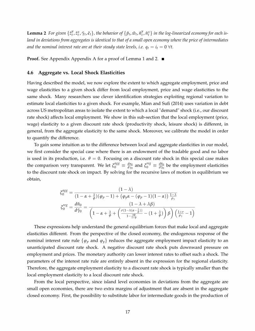
4.6 Aggregate vs. Local Shock Elasticities

Having described the model, we now explore the extent to which aggregate employment, price andwage elasticities to a given shock differ from local employment, price and wage elasticities to thesame shock. Many researchers use clever identification strategies exploiting regional variation toestimate local elasticities to a given shock. For example, Mian and Sufi (2014) uses variation in debtacross US metropolitan areas to isolate the extent to which a local "demand" shock (i.e., our discountrate shock) affects local employment. We show in this sub-section that the local employment (price,wage) elasticity to a given discount rate shock (productivity shock, leisure shock) is different, ingeneral, from the aggregate elasticity to the same shock. Moreover, we calibrate the model in orderto quantify the difference.

To gain some intuition as to the difference between local and aggregate elasticities in our model,we first consider the special case where there is an endowment of the tradable good and no laboris used in its production, i.e. θ = 0. Focusing on a discount rate shock in this special case makesthe comparison very transparent. We let ξ

agg0 ≡ dn0

dγ0and ξ

reg0 ≡ dn0

dγ0be the employment elasticities

to the discount rate shock on impact. By solving for the recursive laws of motion in equilibrium weobtain,

ξagg0 =

(1− λ)

(1− α + λφ )(ϕp − 1) +

(ϕyα− (ϕp − 1)(1− α)

) 1−λργ

ξreg0 =

dn0

dγ0=

(1− λ + λβ)(1− α + λ

φ +

(σ(1−λ(α− 1

φ ))

1− αφ1+φ

− (1 + λφ )

)β

)(1+rργ− 1)

These expressions help understand the general equilibrium forces that make local and aggregateelasticities different. From the perspective of the closed economy, the endogenous response of thenominal interest rate rule {ϕp and ϕy} reduces the aggregate employment impact elasticity to anunanticipated discount rate shock. A negative discount rate shock puts downward pressure onemployment and prices. The monetary authority can lower interest rates to offset such a shock. Theparameters of the interest rate rule are entirely absent in the expression for the regional elasticity.Therefore, the aggregate employment elasticity to a discount rate shock is typically smaller than thelocal employment elasticity to a local discount rate shock.

From the local perspective, since island level economies in deviations from the aggregate aresmall open economies, there are two extra margins of adjustment that are absent in the aggregateclosed economy. First, the possibility to substitute labor for intermediate goods in the production of

17

final consumption goods (β > 0) decreases the regional employment elasticity to the shock (as long

as the term(

σ(1−λ(α− 1φ ))

1− φ1+φ α

− 1)

is positive). Second, the possibility to transfer resources intertempo-

rally through saving/borrowing at the interest rate r, as seen in the term(

1+rργ− 1)

, decreases theregional employment elasticity. Theoretically, therefore, the aggregate employment elasticity to anaggregate discount rate shock can be either greater or smaller than the local employment elasticityto a local discount rate shock.

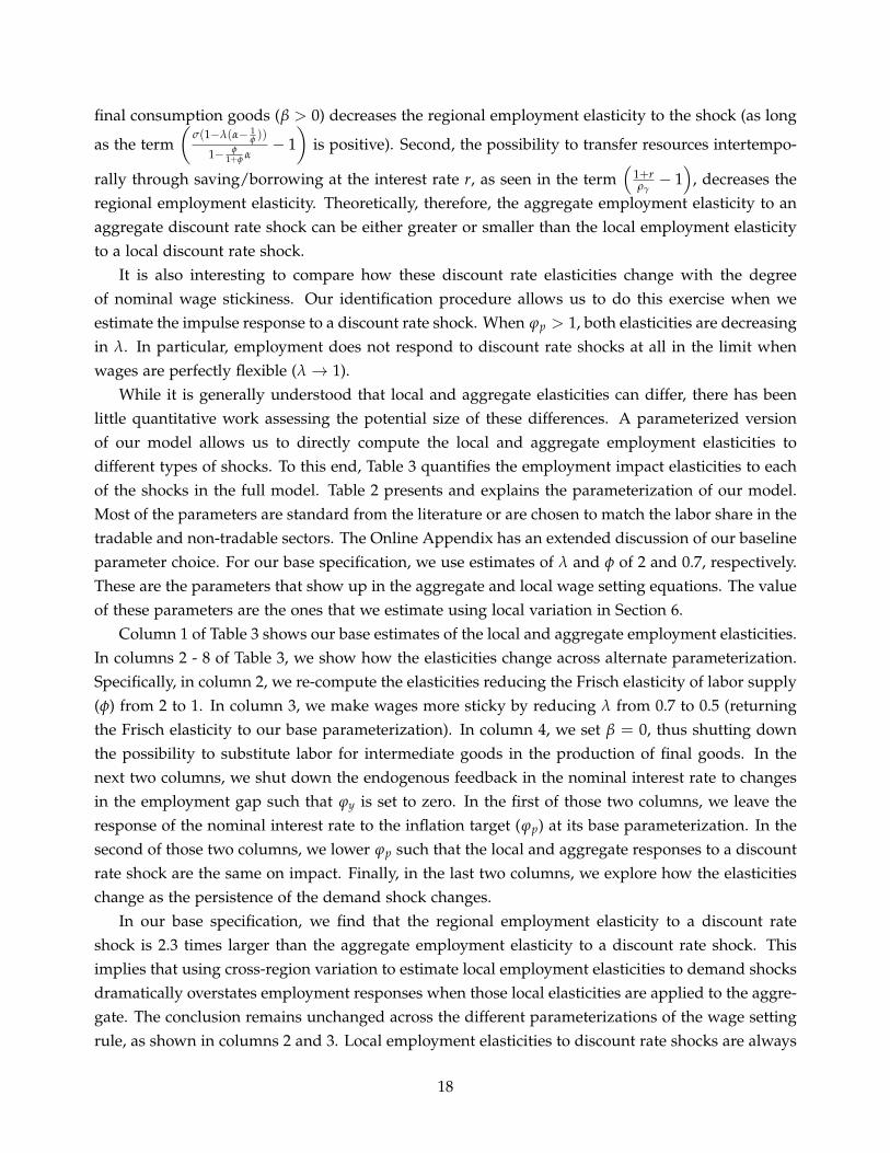
It is also interesting to compare how these discount rate elasticities change with the degreeof nominal wage stickiness. Our identification procedure allows us to do this exercise when weestimate the impulse response to a discount rate shock. When ϕp > 1, both elasticities are decreasingin λ. In particular, employment does not respond to discount rate shocks at all in the limit whenwages are perfectly flexible (λ→ 1).

While it is generally understood that local and aggregate elasticities can differ, there has beenlittle quantitative work assessing the potential size of these differences. A parameterized versionof our model allows us to directly compute the local and aggregate employment elasticities todifferent types of shocks. To this end, Table 3 quantifies the employment impact elasticities to eachof the shocks in the full model. Table 2 presents and explains the parameterization of our model.Most of the parameters are standard from the literature or are chosen to match the labor share in thetradable and non-tradable sectors. The Online Appendix has an extended discussion of our baselineparameter choice. For our base specification, we use estimates of λ and φ of 2 and 0.7, respectively.These are the parameters that show up in the aggregate and local wage setting equations. The valueof these parameters are the ones that we estimate using local variation in Section 6.

Column 1 of Table 3 shows our base estimates of the local and aggregate employment elasticities.In columns 2 - 8 of Table 3, we show how the elasticities change across alternate parameterization.Specifically, in column 2, we re-compute the elasticities reducing the Frisch elasticity of labor supply(φ) from 2 to 1. In column 3, we make wages more sticky by reducing λ from 0.7 to 0.5 (returningthe Frisch elasticity to our base parameterization). In column 4, we set β = 0, thus shutting downthe possibility to substitute labor for intermediate goods in the production of final goods. In thenext two columns, we shut down the endogenous feedback in the nominal interest rate to changesin the employment gap such that ϕy is set to zero. In the first of those two columns, we leave theresponse of the nominal interest rate to the inflation target (ϕp) at its base parameterization. In thesecond of those two columns, we lower ϕp such that the local and aggregate responses to a discountrate shock are the same on impact. Finally, in the last two columns, we explore how the elasticitieschange as the persistence of the demand shock changes.

In our base specification, we find that the regional employment elasticity to a discount rateshock is 2.3 times larger than the aggregate employment elasticity to a discount rate shock. Thisimplies that using cross-region variation to estimate local employment elasticities to demand shocksdramatically overstates employment responses when those local elasticities are applied to the aggre-gate. The conclusion remains unchanged across the different parameterizations of the wage settingrule, as shown in columns 2 and 3. Local employment elasticities to discount rate shocks are always

18

two to three times larger than the aggregate employment elasticities. In columns 4 to 6, we seethe importance of general equilibrium forces. As we shut down the ability to substitute labor forintermediate goods (β = 0), the gap between the regional and aggregate elasticities gets larger. Theability to trade intermediates across regions dampens the local employment elasticity to discountrate (demand) shocks. In columns 5 and 6, we see that the endogenous monetary policy responsealso dramatically dampens the aggregate response to a discount rate shock. This suggests that inperiods where the economy is at the zero lower bound, aggregate and local employment elasticitiesto a demand shock are more similar, a point also made in Nakamura and Steinsson (2014). The lastcolumn explores the sensitivity to changes in the persistence of the discount rate shock. The lesspersistent is the local discount rate shock, the smaller the local employment elasticity because theregions can borrow from and lend to each other. Table 3 also shows the local and aggregate em-ployment response to local and aggregate productivity/markup and leisure shocks. For these twoshocks, the local employment elasticities are usually smaller than their aggregate counterparts. Forthe most part, this results from the particular specification of the nominal interest rate rule. To sum-marize, the quantitative difference between aggregate and local employment elasticities depends onthe type underlying shock and can be quite large.

Tables 4 and 5 summarize the aggregate and regional impulse responses, respectively, for allvariables and shocks in our benchmark calibration. We show results upon impact (the "short-run"elasticities) and after 5 years (the "long-run" elasticities). These tables allow us to assess the model’spredictions. We use the same parameterization as in Table 2. The short run responses in Columns 1of Table 4 and Table 5 just restate the employment elasticities in column 1 of Table 3. The remainderof the tables show the estimates for the price, nominal wage and real wage elasticities to all theunderlying shocks in the model upon impact. As seen from Table 4, an aggregate negative discountrate shock (households become less patient) lowers aggregate employment, lowers aggregate prices,and lowers (slightly) aggregate real wages. Conversely, an aggregate negative productivity shocklowers aggregate employment, raises aggregate prices, and raises aggregate real wages. We will usethe sign of these impact elasticities to help identify the shocks in the SVAR in Section 5.

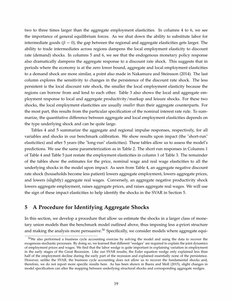
5 A Procedure for Identifying Aggregate Shocks

In this section, we develop a procedure that allow us estimate the shocks in a larger class of mone-tary union models than the benchmark model outlined above, thus imposing less a-priori structureand making the analysis more persuasive.30 Specifically, we consider models where aggregate equi-

30We also performed a business cycle accounting exercise by solving the model and using the data to recover theexogenous stochastic processes. By doing so, we learned that different "wedges" are required to explain the joint dynamicsof employment prices and wages. We find that the labor wedge is quite important in explaining variation in employmentin the early stages of the Great Recession. Like our SVAR results, the Euler equation wedge only explained less thanhalf of the employment decline during the early part of the recession and explained essentially none of the persistence.However, unlike the SVAR, the business cycle accounting does not allow us to recover the fundamental shocks and,therefore, we do not report more specific results here. As has been shown in Buera and Moll (2015), slight changes inmodel specification can alter the mapping between underlying structural shocks and corresponding aggregate wedges.

19

libria can be represented as a structural vector autoregression (SVAR) in price inflation, nominalwage inflation, and employment with three shocks. In order to identify the shocks, we use threeproperties of our benchmark monetary union model: the wage setting equation, the sign of theimpact elasticities to a discount rate and productivity/markup shocks, and the orthogonality ofshocks. Our results will be consistent with monetary union models that satisfy all of these. Beraja(2015) discusses this identification procedure in detail, as well as its application to more generalSVARs and theoretical models than the ones in this paper.

We begin by noting that the recursive solution to the equilibrium system of equations in Lemma1 can be written as a SVAR(∞) in {πt, πw

t , nt}.31

(I − ρ(L))

πt

πwt

nt

= Λ

uεt

uzt

uγt

Knowledge of ρ(L) and an invertible matrix Λ together with aggregate data on prices, nominalwages and employment allow recovering the structural shocks.

The first step in our procedure consists of estimating the reduced form VAR to obtain the autore-gressive matrix ρ(L) and the reduced form errors covariance matrix V. In practice we will truncateρ(L) to be of finite order as it is typically done in the literature. The second step involves derivinga set of theoretical restrictions to identify the structural shocks from the reduced form errors.

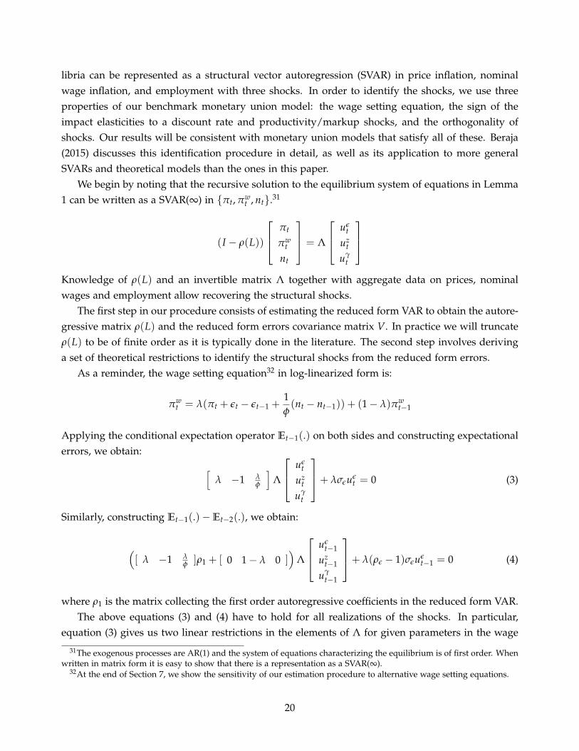
As a reminder, the wage setting equation32 in log-linearized form is:

πwt = λ(πt + εt − εt−1 +

1φ(nt − nt−1)) + (1− λ)πw

t−1

Applying the conditional expectation operator Et−1(.) on both sides and constructing expectationalerrors, we obtain: [

λ −1 λφ

]Λ

uεt

uzt

uγt

+ λσεuεt = 0 (3)

Similarly, constructing Et−1(.)−Et−2(.), we obtain:

([ λ −1 λ

φ ]ρ1 + [ 0 1− λ 0 ])

Λ

uεt−1

uzt−1

uγt−1

+ λ(ρε − 1)σεuεt−1 = 0 (4)

where ρ1 is the matrix collecting the first order autoregressive coefficients in the reduced form VAR.The above equations (3) and (4) have to hold for all realizations of the shocks. In particular,

equation (3) gives us two linear restrictions in the elements of Λ for given parameters in the wage

31The exogenous processes are AR(1) and the system of equations characterizing the equilibrium is of first order. Whenwritten in matrix form it is easy to show that there is a representation as a SVAR(∞).

32At the end of Section 7, we show the sensitivity of our estimation procedure to alternative wage setting equations.

20

setting equation when there are either contemporaneous discount rate or productivity/markupshocks. These two restrictions, together with the six restrictions coming from the orthogonalizationof the shocks, are sufficient to identify the column in the impulse response matrix Λ correspondingto the leisure shock (uε

t ). In order to identify the discount rate and productivity/markup shocks(uγ

t , uzt ) we proceed as follows. From equation (4), we obtain two extra linear restrictions that hold

when there is a lagged discount rate shock or a lagged productivity/markup shock. However, theserestrictions alone cannot "separate" the discount rate from the productivity/markup shocks becausethey are identical for both. Therefore, we use the sign of the impact elasticities from our model toa discount rate and productivity/markup shock (uγ

t and uyt ), respectively. Specifically, we search

over all linear combinations ψ ∈ [0, 1] of the independent restrictions coming from equation (4) suchthat a discount rate (productivity shock/markup) shock: (i) moves prices and employment in thesame (opposite) direction on impact, and (ii) moves real wages and employment in opposite (same)direction on impact. If more than one linear combination of the restrictions satisfy these, we pickthe one that is closer to giving equal weighting to both restrictions.

For completeness, the matrix Λ solves the system:

[λ −1 λ

φ

]Λ

0 01 00 1

= [ 0 0 ]

([ λ −1 λ

φ ]ρ1 + [ 0 1− λ 0 ])

Λ

0ψ

1− ψ

= 0

ΛΛ′ = V

It is worth noting that, when λ = 1, this procedure cannot identify all columns in the impulseresponse matrix Λ because the system above is underdetermined (i.e., (4) implies linear restrictionsthat are merely linear combinations of the restrictions implied by equation (3)). Therefore, somedegree of wage stickiness is key for identification of the shocks through this procedure. The nextsection shows how to estimate λ using regional data—thus linking particular regional patterns toparticular aggregate shock decompositions when combined with the procedure in this section.

6 Estimating the Wage Setting Equation Using Regional Data

In this section, we discuss how we estimate λ and φ which are necessary inputs in our shock iden-tification procedure. Given the above assumptions, the aggregate and local wage setting equationscan be expressed as:

πwt = λ(πt +

1φ(nt − nt−1) + (1− λ)πw

t−1 + λ(uεt − (1− ρε)εt−1)

21

πwkt = λ(πkt +

1φ(nkt − nkt−1)) + (1− λ)πw

kt−1 + λ(uεt − (1− ρε)εt−1) + λvε

kt

The aggregate and local wage setting curves are functions of the Frisch elasticity of labor supply(φ) and the wage stickiness parameter (λ). There is a literature on estimating micro and macro laborsupply elasticities. However, it is hard to estimate the degree of wage stickiness using aggregatedata given the small degrees of freedom inherent to aggregate data and given that at the aggregatelevel it is hard to isolate movements in employment growth and price growth that are arguablyuncorrelated with the aggregate leisure shock (uε

t ). In some instances, regional data can be used toestimate these parameters.

In order for regional data to be used to estimate λ and φ, one of the following must hold: either(1) the leisure shock has no regional component (vε

kt = 0) or (2) the regional component of the leisureshock must be uncorrelated with changes in local economic activity (i.e., cov(vε

kt, (nkt − nkt−1)) = 0and cov(vε

kt, πkt) = 0). The latter condition holds if a valid instrument can be found that isolatesmovement in nkt − nkt−1 and πkt that is orthogonal to vε

kt. In this section, we estimate λ and φ usingregional data on prices, wages and employment growth during the Great Recession. We argue thatstate-level leisure shocks were small during the Great Recession, thus allowing us to estimate λ andφ by OLS. Additionally, we use state-level house price variation during the early part of the GreatRecession as an instrument to isolate movements in nkt − nkt−1 and πkt that are orthogonal to localleisure shocks. Both procedures yield estimates of λ and φ that are fairly similar.

6.1 Estimating Equation and Identification Assumptions

Formally, we estimate the following specification using our state-level data:

πwkt = b0 + b1πkt + b2(nkt − nkt−1) + b3πw

kt−1 + ΨDt + ΓXk + ekt

where b1 = λ, b2 = λ/φ, b3 = (1− λ), and b0 = λ(uεt − (1− ρε)εt−1). Any aggregate leisure shocks

are embedded in the constant term. The local error term includes λvεkt as well as measurement error

for the local economic variables. We estimate this equation pooling together all annual employment,price and wage data for years between 2007 and 2011. When estimating the above regression, weinclude year fixed effects (Dt). This ensures that we are only using the cross-state variation toestimate the parameters. We estimate this equation annually because we only have annual measuresof wages at the state level. Our annual nominal wage measures at the state level are the compositionadjusted nominal log wages computed from the American Community Survey discussed above. πw

kt,therefore, is the log-growth rate in adjusted nominal wages in the state between year t and t− 1.Our measure of employment growth at the state level is calculated using data from the US Bureauof Labor Statistics. The BLS reports annual employment counts and population numbers for eachstate in each year. We divide employment counts by population to make an annual employment ratemeasure for each state. nkt− nkt−1 is the log-change in the employment rate between year t and t− 1.πkt is log-change in the average price index in each state i in year t. In our base specification, we use

22

the retail scanner data local inflation rate scaled to account for the difference between the local non-tradable share in the retail sector and the composite consumption good. In alternative specifications,we use the raw inflation rate from the retail scanner data as our measure of local inflation. Finally,in some specifications, we include controls for the state’s industry mix in 2007. This allows for thepossibility that local leisure shocks, to the extent that they exist, may be correlated with the state’sindustry structure. Given that we have observations on 48 states for 4 years of growth rate data,our estimating equation includes 192 observations in our base specification. We also show resultsrestricting our data to the period from 2007 to 2009, before the large changes in unemploymentbenefits extension starting in 2010.

Two additional comments are needed about our estimating equation. First, the theory developedabove implies that b1 + b3 = 1. We impose this condition when estimating the cross-state regression.Second, we believe our local wage and price indices are measured with error. The measurementerror, if classical, will attenuate our estimates of b1 and b3. Additionally, because we are regressingwage growth on lagged wage growth, any classical measurement error in wages in year t will causea negative relationship between wage growth today and lagged wage growth. We proceed as followsto deal with this issue. Given the large sample sizes on which our wage indices (price indices) arebased, we split the sample in each year and compute two measures of wage indices (price indices)for each state in each year. For example, if we have 1 million observations in the 2007 AmericanCommunity Survey, we split the sample into two distinct samples with 500,000 observations each.Within each sub-sample, we compute a wage measure for each state. Both these wage measures aremeasured with error. Then, we use the growth rates in wages in one sub-sample as an instrumentfor growth rate in wages in the other sub-sample. We discuss these procedure in detail in the OnlineAppendix that accompanies the paper. As we show in that appendix, the procedure corrects theattenuation bias from measurement error in our estimates.33

In order to recover unbiased estimates of λ and φ via OLS, we must assume vεkt = 0. The

assumption that there are no local leisure shocks cannot generically be true. However, in the OnlineAppendix, we provide some evidence suggesting that this assumption may be roughly valid duringthe 2007-2011 period. We show that many potential leisure shocks highlighted in the literature toexplain the Great Recession had large aggregate components but varied little in across US states.For example, the decline in routine jobs (Jaimovich and Siu (2014), Charles et al (2013, 2015)) wasdramatic at the aggregate level during the 2007-2011 period, but occurred in all US states withroughly equal propensity. We show these results in Online Appendix Figure R7. Likewise, somehave argued that the expansion of government policies acted like a leisure shock that discouragedwork (Mulligan (2012)). We show that many of these government policies—such as the expansion ofthe Supplemental Nutrition Assistance Program (SNAP) —was large at the aggregate level but hadlittle cross state variation. In Online Appendix Figure R4, we show that SNAP benefits per recipientincreased by roughly 30 percent between 2007 and 2011. Because the increase in per recipient benefitoccurred at the federal level, there was statutorily no variation in per recipient benefits across US

33This procedure is similar to the split sample instrumental variable estimation in Angrist and Krueger (1995).

23

states during this time period.34

One policy that has received considerable attention in its potential to act as a labor supply shockis the differential extension of the duration of unemployment benefits across states during the GreatRecession. By law in 2010, weeks of unemployment benefits were tied to the state’s unemploymentrate. However, as of 2010, most US states met triggers that resulted in the duration of unemploy-ment benefits being close to the maximum of 99 weeks. These states comprised the bulk of theUS population. However, some smaller states, mostly in the Plains region of the US, had smalleremployment declines and, as a result, had a smaller extension of unemployment benefits.35 Despitethe fact that there was little population-weighted variation across states in unemployment benefitextensions during the Great Recession, we still perform two additional robustness exercises to ac-count for the fact that the small policy differences across states that did occur may have discouragedlabor supply. First, when using our full time period, we exclude any state that had less than 85weeks of unemployment benefit extensions leaving us with a sample of states that had essentiallyno remaining variation in unemployment benefit extensions. Given that the exclude states weresmall in population terms, such exclusion had essentially no effect on our estimates. Additionally,we re-estimate our key parameters using only data prior to 2010. Prior to 2010, the duration ofextended unemployment benefits were the same across all states. We discuss these results below.

While we defend that OLS estimation of the above equation yields unbiased estimates of λ andφ using cross state variation during the Great Recession, it is impossible to completely rule outthat leisure shocks are causing some of the variation in state business cycles during this period.To further explore the robustness of our results, we also estimate IV specifications of the aboveequation. Following the work of many recent papers, including Mian and Sufi (2014), we use con-temporaneous and lagged variation in local house prices as our instruments for local employmentand price growth. The argument is that local house price variation during the 2007-2011 period (inour base specification) or during the 2007-2009 period (in our restricted specification) is orthogonalto movements in local leisure shocks. This seems like a plausible assumption for the 2007-2009period as state policy changes did not occur prior to 2009. In the Online Appendix, we discuss theIV procedure in detail. We also show that contemporaneous housing price growth strongly pre-dicts contemporaneous employment growth and lagged measures of housing growth predicts pricegrowth. We find that IV and OLS estimates are very similar.

Before turning to the estimation, it is also worth discussing the no cross-state migration assump-tion that we have imposed throughout. If individuals were more likely to migrate out of poorperforming states and into better performing states, our estimated labor supply elasticities fromthe state regression may be larger than the aggregate labor supply elasticity. While theoretically

34In the Online Appendix, we also show that there was no systematic variation in state labor income tax rates duringthe 2007-2010 period. Additionally, we show that there was little state variation in Federal programs to help underwaterhomeowners (like HAMP) that occurred during the 2007-2010 period. The reason is that take up rates of the programduring this time period were very low (with take up rates being essentially zero prior to 2010).

35States also had some discretion as to whether they opted into the program. This explains why some states did nothave the maximum weeks of unemployment benefits even when their unemployment rate was higher. We discuss thesepolicies and how they varied across states in detail in the Online Appendix.

24

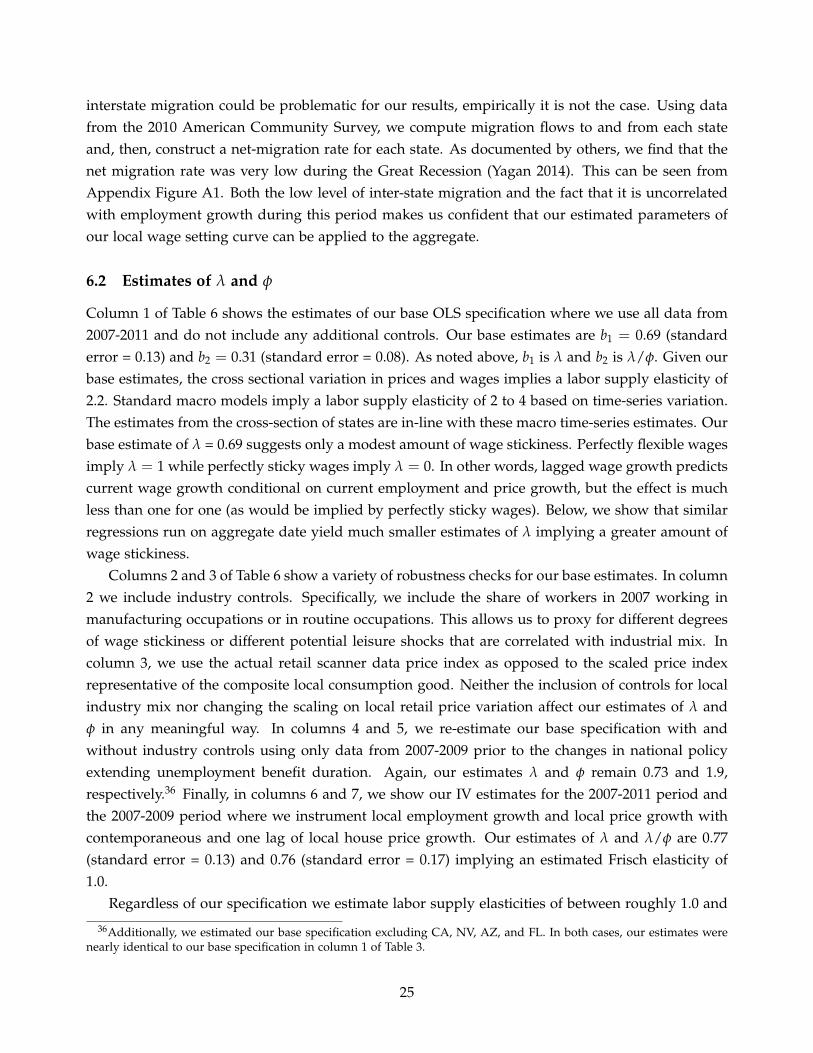
interstate migration could be problematic for our results, empirically it is not the case. Using datafrom the 2010 American Community Survey, we compute migration flows to and from each stateand, then, construct a net-migration rate for each state. As documented by others, we find that thenet migration rate was very low during the Great Recession (Yagan 2014). This can be seen fromAppendix Figure A1. Both the low level of inter-state migration and the fact that it is uncorrelatedwith employment growth during this period makes us confident that our estimated parameters ofour local wage setting curve can be applied to the aggregate.

6.2 Estimates of λ and φ

Column 1 of Table 6 shows the estimates of our base OLS specification where we use all data from2007-2011 and do not include any additional controls. Our base estimates are b1 = 0.69 (standarderror = 0.13) and b2 = 0.31 (standard error = 0.08). As noted above, b1 is λ and b2 is λ/φ. Given ourbase estimates, the cross sectional variation in prices and wages implies a labor supply elasticity of2.2. Standard macro models imply a labor supply elasticity of 2 to 4 based on time-series variation.The estimates from the cross-section of states are in-line with these macro time-series estimates. Ourbase estimate of λ = 0.69 suggests only a modest amount of wage stickiness. Perfectly flexible wagesimply λ = 1 while perfectly sticky wages imply λ = 0. In other words, lagged wage growth predictscurrent wage growth conditional on current employment and price growth, but the effect is muchless than one for one (as would be implied by perfectly sticky wages). Below, we show that similarregressions run on aggregate date yield much smaller estimates of λ implying a greater amount ofwage stickiness.

Columns 2 and 3 of Table 6 show a variety of robustness checks for our base estimates. In column2 we include industry controls. Specifically, we include the share of workers in 2007 working inmanufacturing occupations or in routine occupations. This allows us to proxy for different degreesof wage stickiness or different potential leisure shocks that are correlated with industrial mix. Incolumn 3, we use the actual retail scanner data price index as opposed to the scaled price indexrepresentative of the composite local consumption good. Neither the inclusion of controls for localindustry mix nor changing the scaling on local retail price variation affect our estimates of λ andφ in any meaningful way. In columns 4 and 5, we re-estimate our base specification with andwithout industry controls using only data from 2007-2009 prior to the changes in national policyextending unemployment benefit duration. Again, our estimates λ and φ remain 0.73 and 1.9,respectively.36 Finally, in columns 6 and 7, we show our IV estimates for the 2007-2011 period andthe 2007-2009 period where we instrument local employment growth and local price growth withcontemporaneous and one lag of local house price growth. Our estimates of λ and λ/φ are 0.77(standard error = 0.13) and 0.76 (standard error = 0.17) implying an estimated Frisch elasticity of1.0.

Regardless of our specification we estimate labor supply elasticities of between roughly 1.0 and

36Additionally, we estimated our base specification excluding CA, NV, AZ, and FL. In both cases, our estimates werenearly identical to our base specification in column 1 of Table 3.

25

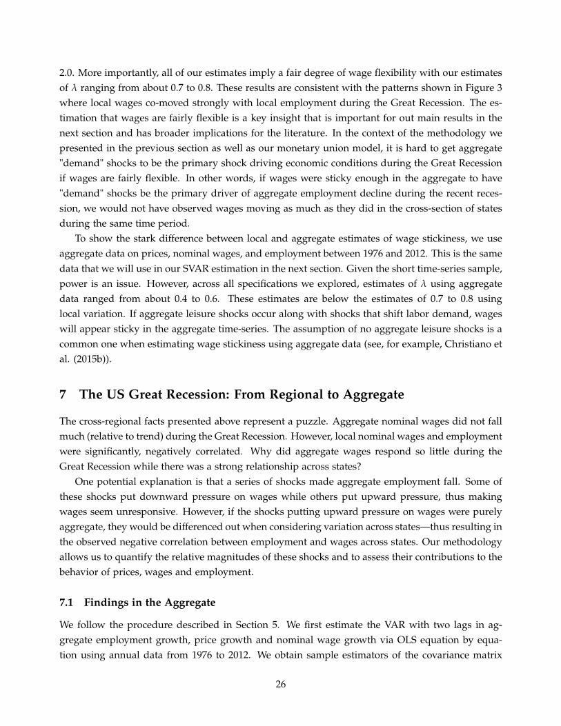
2.0. More importantly, all of our estimates imply a fair degree of wage flexibility with our estimatesof λ ranging from about 0.7 to 0.8. These results are consistent with the patterns shown in Figure 3where local wages co-moved strongly with local employment during the Great Recession. The es-timation that wages are fairly flexible is a key insight that is important for out main results in thenext section and has broader implications for the literature. In the context of the methodology wepresented in the previous section as well as our monetary union model, it is hard to get aggregate"demand" shocks to be the primary shock driving economic conditions during the Great Recessionif wages are fairly flexible. In other words, if wages were sticky enough in the aggregate to have"demand" shocks be the primary driver of aggregate employment decline during the recent reces-sion, we would not have observed wages moving as much as they did in the cross-section of statesduring the same time period.

To show the stark difference between local and aggregate estimates of wage stickiness, we useaggregate data on prices, nominal wages, and employment between 1976 and 2012. This is the samedata that we will use in our SVAR estimation in the next section. Given the short time-series sample,power is an issue. However, across all specifications we explored, estimates of λ using aggregatedata ranged from about 0.4 to 0.6. These estimates are below the estimates of 0.7 to 0.8 usinglocal variation. If aggregate leisure shocks occur along with shocks that shift labor demand, wageswill appear sticky in the aggregate time-series. The assumption of no aggregate leisure shocks is acommon one when estimating wage stickiness using aggregate data (see, for example, Christiano etal. (2015b)).

7 The US Great Recession: From Regional to Aggregate

The cross-regional facts presented above represent a puzzle. Aggregate nominal wages did not fallmuch (relative to trend) during the Great Recession. However, local nominal wages and employmentwere significantly, negatively correlated. Why did aggregate wages respond so little during theGreat Recession while there was a strong relationship across states?

One potential explanation is that a series of shocks made aggregate employment fall. Some ofthese shocks put downward pressure on wages while others put upward pressure, thus makingwages seem unresponsive. However, if the shocks putting upward pressure on wages were purelyaggregate, they would be differenced out when considering variation across states—thus resulting inthe observed negative correlation between employment and wages across states. Our methodologyallows us to quantify the relative magnitudes of these shocks and to assess their contributions to thebehavior of prices, wages and employment.

7.1 Findings in the Aggregate

We follow the procedure described in Section 5. We first estimate the VAR with two lags in ag-gregate employment growth, price growth and nominal wage growth via OLS equation by equa-tion using annual data from 1976 to 2012. We obtain sample estimators of the covariance matrix

26

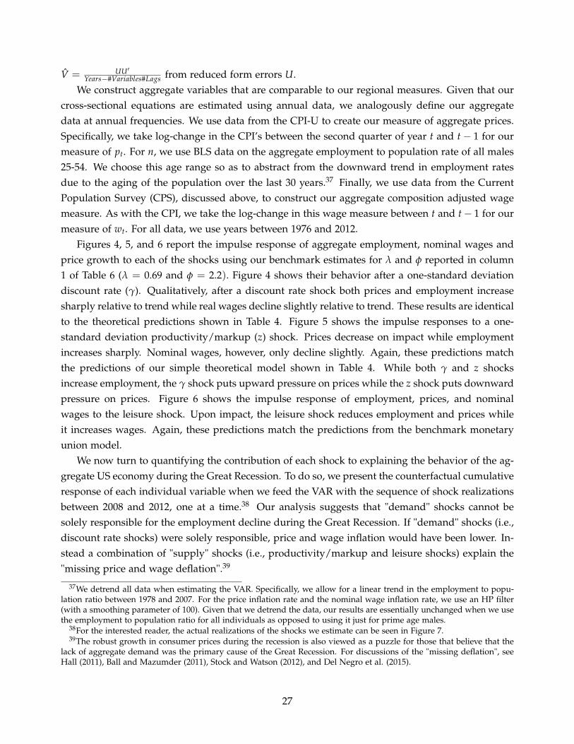
V = UU′Years−#Variables#Lags from reduced form errors U.

We construct aggregate variables that are comparable to our regional measures. Given that ourcross-sectional equations are estimated using annual data, we analogously define our aggregatedata at annual frequencies. We use data from the CPI-U to create our measure of aggregate prices.Specifically, we take log-change in the CPI’s between the second quarter of year t and t− 1 for ourmeasure of pt. For n, we use BLS data on the aggregate employment to population rate of all males25-54. We choose this age range so as to abstract from the downward trend in employment ratesdue to the aging of the population over the last 30 years.37 Finally, we use data from the CurrentPopulation Survey (CPS), discussed above, to construct our aggregate composition adjusted wagemeasure. As with the CPI, we take the log-change in this wage measure between t and t− 1 for ourmeasure of wt. For all data, we use years between 1976 and 2012.

Figures 4, 5, and 6 report the impulse response of aggregate employment, nominal wages andprice growth to each of the shocks using our benchmark estimates for λ and φ reported in column1 of Table 6 (λ = 0.69 and φ = 2.2). Figure 4 shows their behavior after a one-standard deviationdiscount rate (γ). Qualitatively, after a discount rate shock both prices and employment increasesharply relative to trend while real wages decline slightly relative to trend. These results are identicalto the theoretical predictions shown in Table 4. Figure 5 shows the impulse responses to a one-standard deviation productivity/markup (z) shock. Prices decrease on impact while employmentincreases sharply. Nominal wages, however, only decline slightly. Again, these predictions matchthe predictions of our simple theoretical model shown in Table 4. While both γ and z shocksincrease employment, the γ shock puts upward pressure on prices while the z shock puts downwardpressure on prices. Figure 6 shows the impulse response of employment, prices, and nominalwages to the leisure shock. Upon impact, the leisure shock reduces employment and prices whileit increases wages. Again, these predictions match the predictions from the benchmark monetaryunion model.

We now turn to quantifying the contribution of each shock to explaining the behavior of the ag-gregate US economy during the Great Recession. To do so, we present the counterfactual cumulativeresponse of each individual variable when we feed the VAR with the sequence of shock realizationsbetween 2008 and 2012, one at a time.38 Our analysis suggests that "demand" shocks cannot besolely responsible for the employment decline during the Great Recession. If "demand" shocks (i.e.,discount rate shocks) were solely responsible, price and wage inflation would have been lower. In-stead a combination of "supply" shocks (i.e., productivity/markup and leisure shocks) explain the"missing price and wage deflation".39

37We detrend all data when estimating the VAR. Specifically, we allow for a linear trend in the employment to popu-lation ratio between 1978 and 2007. For the price inflation rate and the nominal wage inflation rate, we use an HP filter(with a smoothing parameter of 100). Given that we detrend the data, our results are essentially unchanged when we usethe employment to population ratio for all individuals as opposed to using it just for prime age males.

38For the interested reader, the actual realizations of the shocks we estimate can be seen in Figure 7.39The robust growth in consumer prices during the recession is also viewed as a puzzle for those that believe that the

lack of aggregate demand was the primary cause of the Great Recession. For discussions of the "missing deflation", seeHall (2011), Ball and Mazumder (2011), Stock and Watson (2012), and Del Negro et al. (2015).

27

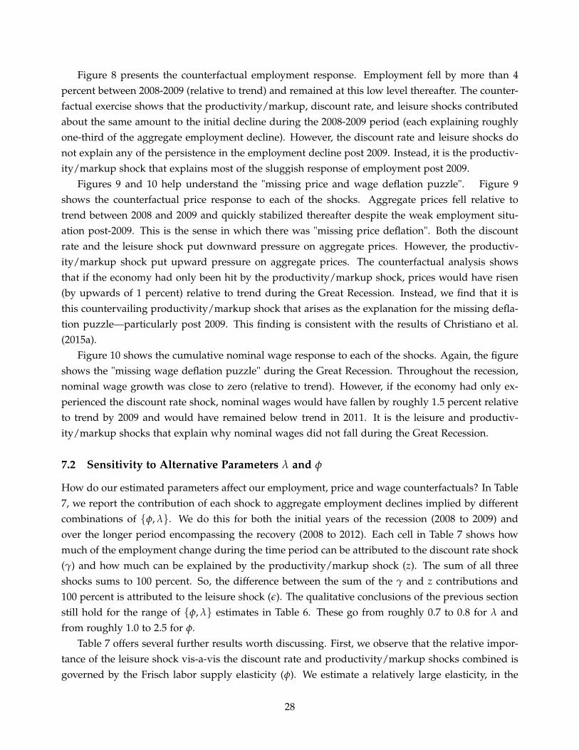
Figure 8 presents the counterfactual employment response. Employment fell by more than 4percent between 2008-2009 (relative to trend) and remained at this low level thereafter. The counter-factual exercise shows that the productivity/markup, discount rate, and leisure shocks contributedabout the same amount to the initial decline during the 2008-2009 period (each explaining roughlyone-third of the aggregate employment decline). However, the discount rate and leisure shocks donot explain any of the persistence in the employment decline post 2009. Instead, it is the productiv-ity/markup shock that explains most of the sluggish response of employment post 2009.

Figures 9 and 10 help understand the "missing price and wage deflation puzzle". Figure 9shows the counterfactual price response to each of the shocks. Aggregate prices fell relative totrend between 2008 and 2009 and quickly stabilized thereafter despite the weak employment situ-ation post-2009. This is the sense in which there was "missing price deflation". Both the discountrate and the leisure shock put downward pressure on aggregate prices. However, the productiv-ity/markup shock put upward pressure on aggregate prices. The counterfactual analysis showsthat if the economy had only been hit by the productivity/markup shock, prices would have risen(by upwards of 1 percent) relative to trend during the Great Recession. Instead, we find that it isthis countervailing productivity/markup shock that arises as the explanation for the missing defla-tion puzzle—particularly post 2009. This finding is consistent with the results of Christiano et al.(2015a).

Figure 10 shows the cumulative nominal wage response to each of the shocks. Again, the figureshows the "missing wage deflation puzzle" during the Great Recession. Throughout the recession,nominal wage growth was close to zero (relative to trend). However, if the economy had only ex-perienced the discount rate shock, nominal wages would have fallen by roughly 1.5 percent relativeto trend by 2009 and would have remained below trend in 2011. It is the leisure and productiv-ity/markup shocks that explain why nominal wages did not fall during the Great Recession.

7.2 Sensitivity to Alternative Parameters λ and φ

How do our estimated parameters affect our employment, price and wage counterfactuals? In Table7, we report the contribution of each shock to aggregate employment declines implied by differentcombinations of {φ, λ}. We do this for both the initial years of the recession (2008 to 2009) andover the longer period encompassing the recovery (2008 to 2012). Each cell in Table 7 shows howmuch of the employment change during the time period can be attributed to the discount rate shock(γ) and how much can be explained by the productivity/markup shock (z). The sum of all threeshocks sums to 100 percent. So, the difference between the sum of the γ and z contributions and100 percent is attributed to the leisure shock (ε). The qualitative conclusions of the previous sectionstill hold for the range of {φ, λ} estimates in Table 6. These go from roughly 0.7 to 0.8 for λ andfrom roughly 1.0 to 2.5 for φ.

Table 7 offers several further results worth discussing. First, we observe that the relative impor-tance of the leisure shock vis-a-vis the discount rate and productivity/markup shocks combined isgoverned by the Frisch labor supply elasticity (φ). We estimate a relatively large elasticity, in the

28

range of that used to calibrate standard macro models.40 However, suppose we used a much lowerelasticity instead, e.g., φ = 0.5, which is in line with some microeconomic estimates in the literature.In this case, the leisure shock would account for a much larger fraction of the employment declinein the Great Recession. In other words, if labor supply is fairly elastic, large movements in em-ployment are consistent with relatively small movements in real wages (as we observe in US data),without the need of large leisure shocks. While this sensitivity analysis results from re-estimatingthe shocks under different parameterizations for φ using our procedure, the intuition is in line withthe benchmark monetary union model from Section 4.

The intuition for the decomposition between discount rate and productivity/markup shocks ismore subtle but also in line with the our benchmark monetary union model. We find that the degreeof wage flexibility (λ) affects their relative contribution to the remaining, unexplained part by theleisure shock alone. For example, if we increased the degree of wage flexibility,41 the productiv-ity/markup shock would account for a much larger fraction of the employment decline in the GreatRecession. Theoretically, it is clear that when λ is large, the discount rate shock should not mattermuch for the determination of employment. To see this, consider the extreme case where wagesare perfectly flexible and the discount rate shock is only composed of the monetary shock. Thenthe equilibrium in the simple theoretical model satisfies monetary neutrality. We formalized thispoint in Section 4.6 when we derived the model’s implied elasticity of aggregate employment to adiscount rate shock. Conversely, when wages are very rigid (λ = 0.1), our procedure suggest thatdiscount rate shocks explain essentially all of the decline in the early part of the recession and muchof the persistence in employment decline during the 2008-2012 period.

7.3 Sensitivity to Alternative Identifying Assumptions

The above results are based on the particular functional form of our wage setting equation:

Wkt = (Pkteεkt(Nkt)1φ )λ (Wkt−1)

1−λ

This wage setting equation reflects our assumption of GHH preferences as well as no forwardlooking behavior when wages are reset. Both of these assumptions were made for tractability. Inthis sub-section, we explore the sensitivity of our results to relaxing both of these assumptions.

In Appendix B1, we derive the aggregate and local wage setting equations under a broad set ofutility functions where consumption and leisure are non-separable. This class of utility functions

40This result may be of independent interest to the reader familiar with the macro v. micro labor supply elasticities (seeChetty, Guren, Manoli, and Weber (2011)). Using cross-sectional data (same as in most of the micro labor-supply elasticityliterature) we arrive at an estimate similar to the macro elasticity (estimated from aggregate time-series data). We believethis is because the regional variation in employment rates that we use to estimate this elasticity only incorporates theextensive margin adjustment in the labor supply, which is the same margin that is most important in accounting foraggregate fluctuations in total hours over the business cycle.

41It is worth mentioning that for large values of λ and small values of φ, the results in Table 7 become rather sensitiveto small variations in parameters. This is because our shock identification procedure needs a certain degree of wagestickiness, as explained in the Section 5. For example, for values of λ around 0.95 it is not possible to identify theproductivity/markup and discount rate shocks.

29

allows for arbitrarily large income and substitution effects. As we show in the appendix, the use oflocal consumption data allows us to estimate the extent of wage stickiness as well as to estimate theparameters that encompass both the income and substitution effects on labor supply. In particular,we can estimate the following equation using local data:

πwkt = bt + b1πkt + b2(nkt − nkt−1 + b3πw

kt−1 + b4(ckt − ckt−1) + ΨDt + ΓXk + ekt.

This equation is identical to our estimating equation above aside from the addition of localconsumption growth (i.e., ckt− ckt−1) . As outlined in Appendix B1, the coefficients b1 and b3 sum to1 even under the broader preference specification. We impose this restriction when estimating themodified equation. We measure local real consumption growth using the log-change in real retailexpenditures at the state level computed within the Nielsen sample. We obtain real expendituresby deflating nominal expenditures with our local price indices.42 For our base specification, ourestimates of b1, b2, and b4 are 0.72 (standard error = 0.12), 0.25 (standard error = 0.08), and 0.16(standard error = 0.06), respectively. A positive and significant coefficient on real consumptiongrowth (b4) reflects the presence of income effects on labor supply. Controlling for this incomeeffect, our estimate of wage flexibility (b1) is slightly higher than our base specification where incomeeffects are not allowed.

In the aggregate wage setting equation, we can substitute out consumption growth using themodel definition (ct = wt + nt − pt). Appendix B1 shows that the aggregate wage setting equationstill takes the following form:

πwt = λπt +

λ

φ(nt − nt−1) + (1− λ)πw

t−1 +λ

1−ωεt

where ω is a parameter that represents the strength of the income effect on labor supply (andmaps directly to b4 from the above local labor supply regression, see equation (5) in AppendixB1). Aside from the coefficient scaling the aggregate leisure shock, this equation is identical to theidentification restriction we imposed when estimating the aggregate SVAR. The only difference isthat there is no longer a direct mapping between λ and λ/φ—in the above aggregate wage settingequation that we impose to identify the SVAR—and the reduced-form parameters b1 and b2—in thelocal wage setting equation. However, as shown in Appendix B1, there is still a one-to-one mappingbetween the parameters we estimate from the local regression (b1, b2, and b4) and the aggregate pa-rameters we need to identify the SVAR (λ and φ). With the correctly specified λ and φ, we can justuse the matrix in Table 7 to read off the decomposition of shocks during the Great Recession. Whileλ and φ are no longer structural parameters (instead being combinations of structural parameters),knowing them still helps identifying the aggregate SVAR. Using our estimates of b1, b2, and b4 andthe procedure developed in Appendix B1, we estimate λ and φ (allowing for income effects on labor

42This measure of real expenditures is (1) highly correlated with measures of local employment and (2) highly correlatedwith the BEA’s recent state level personal expenditures measure. Our results are similar if we use the BEA’s localconsumption measure. However, we prefer our measure given that much of the BEA’s local consumption measure isimputed (where the imputation uses local employment measures).

30

supply) to be 0.68 and 2.0, respectively. These parameters are nearly identical to our base specifi-cation without income effects. The take-away from this sensitivity exercise is that abstracting fromincome effects on labor supply is not biasing our decomposition of the shocks driving aggregateemployment declines during the Great Recession in any meaningful way.

In Appendix B2, we specify an alternative wage setting equation allowing for forward lookingbehavior when wages are reset. We show that ignoring forward looking wage setting behavior biasesup our estimates of wage flexibility. That is, the amount of wage flexibility that we estimate usingcross-state variation is too large relative to the true amount of wage flexibility in the aggregate. Weshow that the bias depends on two parameters: (1) the extent to which firms put weight on forwardlooking behavior when setting wages (which we call κ) and (2) the underlying persistence processof local wages (which we call ρw). Assuming that at the aggregate level the monetary authoritywants to stabilize expected nominal wage growth, we quantify the extent to which our estimatesof λ from the local regressions are biased upwards as a function of these two parameters. Under arange of plausible parameter estimates for κ and ρw, we show that the bias is quite small. For ourbaseline parameter estimates, we show that κ(1− ρw) must exceed 2.5 for the true λ to be lowerthan 0.4. This is an order of magnitude larger than any plausible parametrization for either κ or ρw.Moreover, as seen in Table 7, our estimates of the role of demand shocks in explaining employmentdecline during the Great Recession are broadly similar for values of λ between 0.4 and 0.69. Theseresults suggest that our abstraction from including expectations in our wage setting equation is notquantitatively altering the paper’s conclusions.

7.4 Discussion: Aggregate v. Regional Shock Decomposition

The above results suggest that aggregate wages appeared sticky during the Great Recession becausea combination of aggregate shocks resulted in relatively offsetting effects on aggregate wages. Byextending our procedure to allow for the estimation of regional shocks in a regional SVAR, wefind that that the discount rate shock explains roughly 80 percent of the change in non-tradableemployment between 2007 and 2010 across states. This is consistent with results found in Mian andSufi (2014) suggesting that housing price declines explained much of the cross-state variation in non-tradable employment. We conclude that even though discount rate shocks only explained a portionof aggregate employment decline early in the Great Recession and very little of its persistence, thediscount rate shock was primarily responsible for much of the cross-state variation during this timeperiod.

We relegate the discussion of the estimation procedure and identification assumptions to theOnline Appendix—given that the estimation of regional shocks is not central to the paper. However,this exercise allow us to highlight the difficulty in extrapolating findings from cross-region variationto interpret aggregate time-series patterns. The fact that local discount rate shocks explain much ofthe cross-state variation in employment during the Great Recession does not imply that an aggre-gate discount rate shock explains much of the aggregate time-series variation in employment duringthe Great Recession. If the discount rate shock would have been the main driver of aggregate em-

31

ployment decline during the Great Recession then aggregate wages would have behaved similarlyto state-level wages.

8 Conclusion

Regional business cycles during the Great Recession in the US were strikingly different than theiraggregate counterpart. This is the cornerstone observation on which we built this paper. Yet, theaggregate US economy is just a collection of these regions connected by trade of goods and assets.We argued that their aggregation cannot be arbitrary and that regional business cycle patterns haveinteresting implications for aggregate business cycles.

Our paper offers four takeaways. The first is that the relationship between wages and employ-ment in the aggregate time-series during the 2006-2011 period is very different than the cross-staterelationship between these variables during the same time period. For example, while aggregatewages appeared to be sticky despite aggregate employment falling sharply, both local nominal andreal wages co-varied strongly with local employment growth in the cross-section of US states. Bothdocumenting the regional facts and the creation of the underlying local price and wage indices arethe first innovations of the paper.

The second take-away is that wages seem to be modestly sticky when using cross-state variationto estimate our wage setting equation. The amount of wage stickiness is often a key parameter inmany macro models. Despite its importance, there are not many estimates of the frequency withwhich wages adjust (particularly relative to estimates of price adjustments). We develop a procedureto estimate the amount of wage stickiness using cross-region variation. The wage stickiness param-eter is key to our empirical methodology to estimate the underlying shocks and elasticities. The factthat we estimate that wages are only modestly sticky limits the importance of "demand" shocks atthe aggregate level in explaining the Great Recession. If wages are only modestly sticky, aggregatedemand shocks should have resulted in falling aggregate wages—which was not observed in theaggregate time-series. Regardless of the use of this parameter in our empirical work, our estimateof wage stickiness could be of independent interest to researchers.

The third take-away from this paper is developing a methodology that allows us to estimateaggregate shocks by combining aggregate and regional data. This methodology is a hybrid methodthat merges restrictions imposed by a theoretical model with aggregate and cross-sectional datawhen estimating a SVAR and identifying the corresponding shocks. We view this as a contributionto the growing literature that uses model-based structure to estimate SVARs.

Finally, the fourth take-away is perhaps the most important for the goals of the paper. We showthat a combination of both "demand" and "supply" shocks are necessary to account for the jointdynamics of aggregate prices, wages and employment during the 2007-2012 period in the US. Incontrast with the aggregate results, we find that discount rate shocks explain most of the observedemployment, price and wage dynamics across states. These results suggest that solely using cross-region variation to explain aggregate fluctuations is insufficient when some shocks do not have a

32

substantive regional component. The fact that aggregate wages did not fall cannot be explainedby large degrees of wages stickiness. The reason aggregate wages did not fall is that the series ofshocks experienced by the aggregate economy were such that some shocks put downward pressureon prices and wages (discount rate shocks) while other shocks put upward pressure on pricesand wages (productivity/markup and leisure shocks). In the cross-section, however, the discountrate shocks caused prices, wages and employment to move in the same direction. Lastly, in ourcalibrated monetary union model, we show that the local employment elasticity to a local discountrate shock is substantially larger than the aggregate employment elasticity to an identically-sizedaggregate discount rate shock. These results suggest that even when the aggregate and regionalshocks are the same, it is hard to draw inferences about the aggregate economy using regionalvariation. Collectively, our results suggest that researchers should be cautious when extrapolatingcross-sectional variation to make statements about aggregate business cycles.

33

References

An, Sungbae and Frank Schorfheide, 2007. “Bayesian Analysis of DGSE Models”, Econometric Reviews, 24(2-4), 113-73. Autor, David, David Dorn, and Gordon Hanson, 2013. "The China Syndrome: Local Labor Market Effects of Import Competitions in the United States", American Economic Review, 103(6), 2121-2168. Ball, Laurence and Sandeep Mazumder, 2011. “Inflation Dynamics and the Great Recession”, Brookings Papers on Economic Activity, 42(1), 337-405. Beraja, Martin, 2015. “A Semi-Structural Methodology for Policy Counterfactuals and an Application to Fiscal Unions”, University of Chicago Working Paper. Berger, David and Joe Vavra, 2015. “Dynamics of the U.S. Price Distribution”, Working Paper. Buera, Francisco and Benjamin Moll, 2015. “Aggregate Implications of a Credit Crunch: The Importance of Heterogeneity”, American Economic Journal: Macroeconomics, 7(3), 1-42. Blanchard, Olivier and Lawrence Katz, 1991. "Regional Evolutions", Brookings Papers on Economic Activity, 1992:1, 1-75. Cage, Robert, John Greenless and Patrick Jackman, 2003. “Introducing the Chained Consumer Price Index,” U.S. Bureau of Labor Statistics. Carriero, Andrea and Raffaella Giacomini, 2011. “How Useful are No-Arbitrage Restrictions for Forecasting the Term Structure of Interest Rates”, Journal of Econometrics, 164(1), 21-34. Charles, Kerwin, Erik Hurst, and Matthew Notowidigdo, 2015. "Masking and Employment Changes During the 2000s: Housing Booms and Manufacturing Decline”, University of Chicago Working Paper. Charles, Kerwin, Erik Hurst, and Matthew Notowidigdo, 2013. "Manufacturing Decline, Housing Booms and Non-Employment", NBER Working Paper #18989. Chetty, Raj, Adam Guren, Day Manoli, and Andrea Weber, 2011. “Are Micro and Macro Labor Supply Elasticities Consistent? A Review of Evidence on the Intensive and Extensive Margins”, American Economic Review Papers and Proceedings, 471-5. Christiano, Lawrence, Martin Eichenbaum, and Mathias Trabandt, 2015a. “Understanding the Great Recession” American Economic Journal - Macro, January, 110-67. Christiano, Lawrence, Martin Eichenbaum, and Mathias Trabandt, 2015b. "Unemployment and Business Cycles", Econometrica (forthcoming).

Coibion, Olivier, Yuriy Gorodnichenko, and Gee Hee Hong, 2015. "The Cyclicality of Sales, Regular and Effective Prices: Business Cycle and Policy Implications", American Economic Review, 105(3), 993-1029. Del Negro, Marco and Frank Schorfheide, 2004. “Priors from General Equilibrium Models for VARs”, International Economic Review, 45, 643-73. Del Negro, Marco, Marc Giannoni, and Frank Schorfheide, 2015. “Inflation in the Great Recession and New Keynesian Models”, American Economic Journal: Macroeconomics, 7(1): 168-96. Diewert, Erwin W., 1976. "Exact and Superlative Index Numbers," Journal of Econometrics 46, 115–45. Diewert, Erwin W., Lorraine Ivancic and Kevin J. Fox, 2011. “Scanner data, time aggregation and the construction of price indexes,” Journal of Econometrics 161, 24-35. Eggertsson, Gauti and Paul Krugman, 2012. “Debt, Deleveraging, and the Liquidity Trap: A Fisher-Minsky-Koo Approach”, Quarterly Journal of Economics, 127(3), 1469-513. Fitzgerald, Terry and Juan Pablo Nicolini, 2014. “Is there a Stable Relationship Between Unemployment and Future Inflation? Evidence from U.S. Cities”, Federal Reserve Bank of Minneapolis Working Paper 713. Gali, Jordi, 2011. “Monetary Policy and Unemployment”, Handbook of Monetary Economics, vol. 3A, Elsevier B.V., 487-546 Giroud, Xavier and Holger Mueller, 2015. “Firm Leverage and Unemployment during the Great Recession”, Working Paper Gilchrist, Simon, Raphael Schoenle, Jae Sim, and Egon Zakrajsek, 2014. “Inflation Dynamics During the Financial Crisis”, working paper. Guerrieri, Veronica and Guido Lorenzoni, 2011. “Credit Crises, Precautionary Savings and the Liquidity Trap”, University of Chicago Working Paper. Hagerdon, Marcus, Fatih Karahan, Iourii Manovskii, and Kurt Mitman, 2015. “Unemployment Benefits and Unemployment in the Great Recession: The Role of Macro Effects” NBER Working Paper 19499. Hall, Robert, 2011. “The Long Slump”, American Economic Review, 101(2), 431-469. Hall, Robert and Paul Milgrom, 2008. “The Limited Influence of Unemployment on the Wage Bargain”, American Economic Review, 98(4), 1653-74.

Baumeister, Christiane and James Hamilton (2015). “Sign Restrictions, Structural Vector Autoregressions, and Useful Prior Information”, Econometrica, 83, 1963-99. Jaimovich, Nir and Henry Siu, 2014. “The Trend is the Cycle: Job Polarization and Jobless Recoveries”, Duke University Working Paper. Kaplan, Greg and Guido Menzio, 2015. "The Morphology of Price Dispersion", International Economic Review, forthcoming. Mehrotra, Neil and Dmitriy Sergeyev, 2015. “Financial Shocks and Job Flows”, Brown University Working Paper. Melser, Daniel, 2011. “Constructing High Frequency Price Indexes Using Scanner Data,” Working Paper, 2011 Mian, Atif and Amir Sufi, 2014. "What Explains the High Unemployment? The Aggregate Demand Channel", Econometrica (forthcoming) Mian, Atif, Kamalesh Rao, and Amir Sufi, 2013. "Household Balance Sheets, Consumption and The Economic Slump", Quarterly Journal of Economics, 1687-1726. Mian, Atif and Amir Sufi, 2011. "House Prices, Home Equity-Based Borrowing, and the U.S. Household Leverage Crisis", American Economic Review, 101(4), 2132-56. Midrigan, Virgiliu and Thomas Philippon, 2011. "Household Leverage and the Recession", NYU Working Paper. Mondragron, John, 2015. “Household Credit and Employment in the Great Recession”, University of California at Berkeley Working Paper. Mulligan, Casey, 2012. “The Redistribution Recession: How Labor Market Distortions Contracted the Economy”, Oxford University Press. Nakamura, E. and J. Steinsson (2014). “Fiscal Stimulus in a Monetary Union: Evidence from US Regions,” The American Economic Review, 104, 753–792. Ruggles, Steven, J. Trent Alexander, Katie Genadek, Ronald Goeken, Matthew B. Schroeder, and Mathew Sobek, 2010. Integrated Public Use Microdata Series: Version 5.0. Minneapolis: University of Minnesota. Schmitt-Grohé, S. and M. Uribe, 2003: “Closing small open economy models,” Journal of International Economics, 61, 163–185. Schorfheide, Frank, 2000. “Loss Function-based Evaluation of DSGE Models”, Journal of Applied Econometrics, 15(6), 645-70.

Shimer, Robert, 2010. Labor Markets and Business Cycles, Princeton University Pres. Stock, James and Mark Watson, 2012. “Disentangling the Channels of the 2007-2009 Recession”, Brookings Papers on Economic Activity, Spring (2012). Stroebel, Johannes and Joseph Vavra, 2014. “House Prices, Local Demand, and Retail Prices”, NBER Working Paper, 20710. Vavra, Joseph, 2014. “Inflation Dynamics and Time Varying Volatility: New Evidence and an Ss Interpretation”, Quarterly Journal of Economics, 129(1). Yagan, Danny, 2014. “Moving to Opportunity? Migratory Insurance Over the Great Recession”, Working Paper.

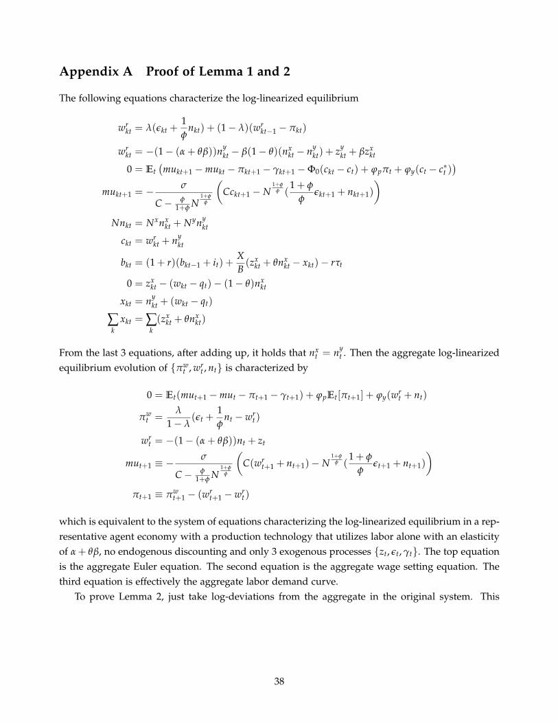
Appendix A Proof of Lemma 1 and 2

The following equations characterize the log-linearized equilibrium

wrkt = λ(εkt +

1φ

nkt) + (1− λ)(wrkt−1 − πkt)

wrkt = −(1− (α + θβ))ny

kt − β(1− θ)(nxkt − ny

kt) + zykt + βzx

kt

0 = Et(mukt+1 −mukt − πkt+1 − γkt+1 −Φ0(ckt − ct) + ϕpπt + ϕy(ct − c∗t )

)mukt+1 = − σ

C− φ1+φ N

1+φφ

(Cckt+1 − N

1+φφ (

1 + φ

φεkt+1 + nkt+1)

)Nnkt = Nxnx

kt + Nynykt

ckt = wrkt + ny

kt

bkt = (1 + r)(bkt−1 + it) +XB(zx

kt + θnxkt − xkt)− rτt

0 = zxkt − (wkt − qt)− (1− θ)nx

kt

xkt = nykt + (wkt − qt)

∑k

xkt = ∑k(zx

kt + θnxkt)

From the last 3 equations, after adding up, it holds that nxt = ny

t . Then the aggregate log-linearizedequilibrium evolution of {πw

t , wrt , nt} is characterized by

0 = Et(mut+1 −mut − πt+1 − γt+1) + ϕpEt[πt+1] + ϕy(wrt + nt)

πwt =

λ

1− λ(εt +

1φ

nt − wrt)

wrt = −(1− (α + θβ))nt + zt

mut+1 ≡ −σ

C− φ1+φ N

1+φφ

(C(wr

t+1 + nt+1)− N1+φ

φ (1 + φ

φεt+1 + nt+1)

)πt+1 ≡ πw

t+1 − (wrt+1 − wr

t)

which is equivalent to the system of equations characterizing the log-linearized equilibrium in a rep-resentative agent economy with a production technology that utilizes labor alone with an elasticityof α + θβ, no endogenous discounting and only 3 exogenous processes {zt, εt, γt}. The top equationis the aggregate Euler equation. The second equation is the aggregate wage setting equation. Thethird equation is effectively the aggregate labor demand curve.

To prove Lemma 2, just take log-deviations from the aggregate in the original system. This

38

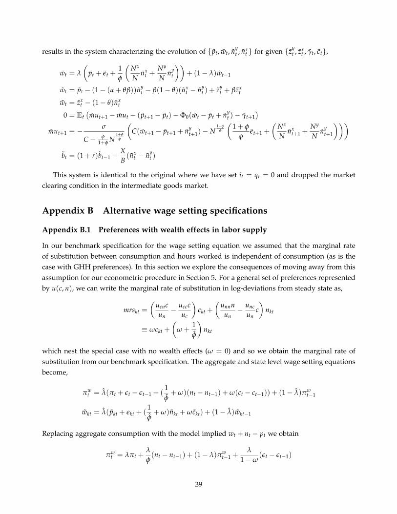
results in the system characterizing the evolution of { pt, wt, nyt , nx

t } for given {zyt , zx

t , γt, εt},

wt = λ

(pt + εt +

1φ

(Nx

Nnx

t +Ny

Nny

t

))+ (1− λ)wt−1

wt = pt − (1− (α + θβ))nyt − β(1− θ)(nx

t − nyt ) + zy

t + βzxt

wt = zxt − (1− θ)nx

t

0 = Et(mut+1 − mut − ( pt+1 − pt)−Φ0(wt − pt + ny

t )− γt+1)

mut+1 ≡ −σ

C− φ1+φ N

1+φφ

(C(wt+1 − pt+1 + ny

t+1)− N1+φ

φ

(1 + φ

φεt+1 +

(Nx

Nnx

t+1 +Ny

Nny

t+1

)))

bt = (1 + r)bt−1 +XB(nx

t − nyt )

This system is identical to the original where we have set it = qt = 0 and dropped the marketclearing condition in the intermediate goods market.

Appendix B Alternative wage setting specifications

Appendix B.1 Preferences with wealth effects in labor supply

In our benchmark specification for the wage setting equation we assumed that the marginal rateof substitution between consumption and hours worked is independent of consumption (as is thecase with GHH preferences). In this section we explore the consequences of moving away from thisassumption for our econometric procedure in Section 5. For a general set of preferences representedby u(c, n), we can write the marginal rate of substitution in log-deviations from steady state as,

mrskt =

(ucncun− uccc

uc

)ckt +

(unnn

un− unc

unc)

nkt

≡ ωckt +

(ω +

1φ

)nkt

which nest the special case with no wealth effects (ω = 0) and so we obtain the marginal rate ofsubstitution from our benchmark specification. The aggregate and state level wage setting equationsbecome,

πwt = λ(πt + εt − εt−1 + (

1φ+ ω)(nt − nt−1) + ω(ct − ct−1)) + (1− λ)πw

t−1

wkt = λ( pkt + εkt + (1φ+ ω)nkt + ωckt) + (1− λ)wkt−1

Replacing aggregate consumption with the model implied wt + nt − pt we obtain

πwt = λπt +

λ

φ(nt − nt−1) + (1− λ)πw

t−1 +λ

1−ω(εt − εt−1)

39

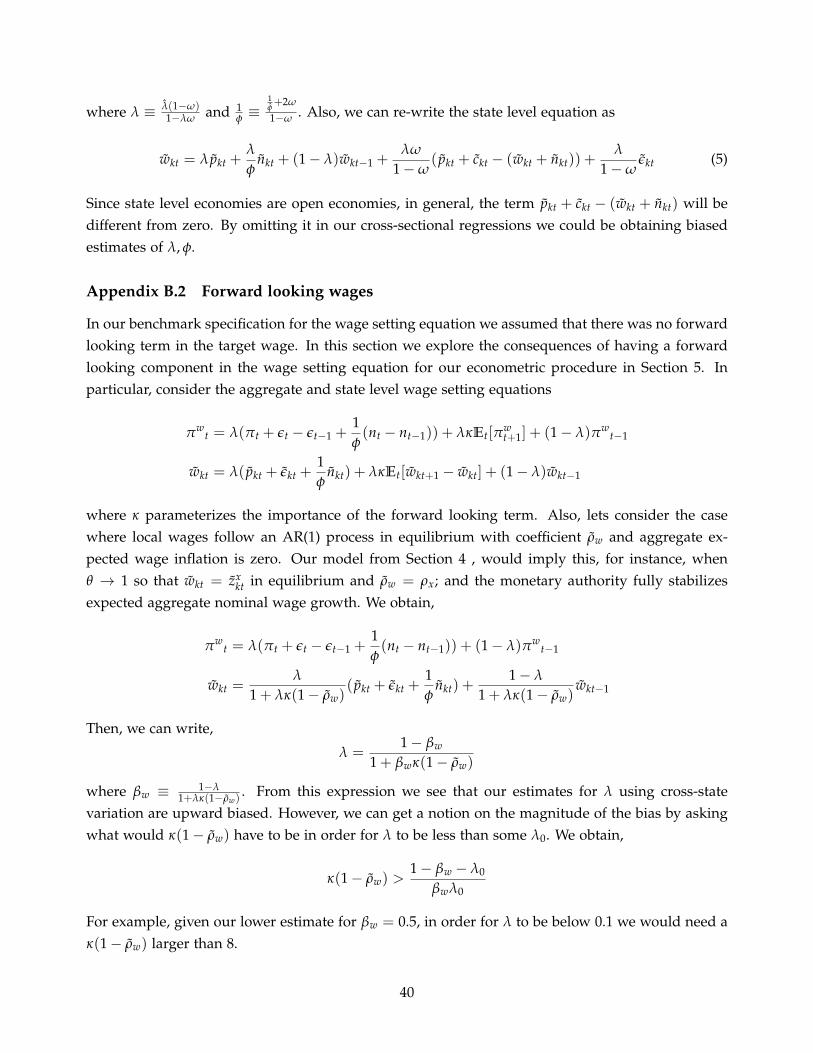
where λ ≡ λ(1−ω)1−λω and 1

φ ≡1φ+2ω

1−ω . Also, we can re-write the state level equation as

wkt = λ pkt +λ

φnkt + (1− λ)wkt−1 +

λω

1−ω( pkt + ckt − (wkt + nkt)) +

λ

1−ωεkt (5)

Since state level economies are open economies, in general, the term pkt + ckt − (wkt + nkt) will bedifferent from zero. By omitting it in our cross-sectional regressions we could be obtaining biasedestimates of λ, φ.

Appendix B.2 Forward looking wages

In our benchmark specification for the wage setting equation we assumed that there was no forwardlooking term in the target wage. In this section we explore the consequences of having a forwardlooking component in the wage setting equation for our econometric procedure in Section 5. Inparticular, consider the aggregate and state level wage setting equations

πwt = λ(πt + εt − εt−1 +

1φ(nt − nt−1)) + λκEt[π

wt+1] + (1− λ)πw

t−1

wkt = λ( pkt + εkt +1φ

nkt) + λκEt[wkt+1 − wkt] + (1− λ)wkt−1

where κ parameterizes the importance of the forward looking term. Also, lets consider the casewhere local wages follow an AR(1) process in equilibrium with coefficient ρw and aggregate ex-pected wage inflation is zero. Our model from Section 4 , would imply this, for instance, whenθ → 1 so that wkt = zx

kt in equilibrium and ρw = ρx; and the monetary authority fully stabilizesexpected aggregate nominal wage growth. We obtain,

πwt = λ(πt + εt − εt−1 +

1φ(nt − nt−1)) + (1− λ)πw

t−1

wkt =λ

1 + λκ(1− ρw)( pkt + εkt +

1φ

nkt) +1− λ

1 + λκ(1− ρw)wkt−1

Then, we can write,

λ =1− βw

1 + βwκ(1− ρw)

where βw ≡ 1−λ1+λκ(1−ρw)

. From this expression we see that our estimates for λ using cross-statevariation are upward biased. However, we can get a notion on the magnitude of the bias by askingwhat would κ(1− ρw) have to be in order for λ to be less than some λ0. We obtain,

κ(1− ρw) >1− βw − λ0

βwλ0

For example, given our lower estimate for βw = 0.5, in order for λ to be below 0.1 we would need aκ(1− ρw) larger than 8.

40

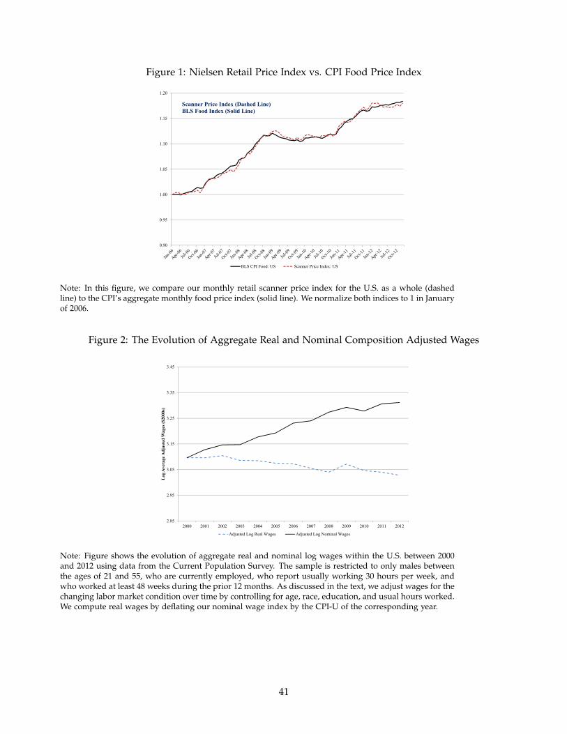
Figure 1: Nielsen Retail Price Index vs. CPI Food Price Index

0.90

0.95

1.00

1.05

1.10

1.15

1.20

BLS CPI Food: US Scanner Price Index: US

Scanner Price Index (Dashed Line)BLS Food Index (Solid Line)

Note: In this figure, we compare our monthly retail scanner price index for the U.S. as a whole (dashedline) to the CPI’s aggregate monthly food price index (solid line). We normalize both indices to 1 in Januaryof 2006.

Figure 2: The Evolution of Aggregate Real and Nominal Composition Adjusted Wages

2.85

2.95

3.05

3.15

3.25

3.35

3.45

2000 2001 2002 2003 2004 2005 2006 2007 2008 2009 2010 2011 2012

Log

Ave

rage

Adj

uste

d W

ages

($20

00s)

Adjusted Log Real Wages Adjusted Log Nominal Wages

Note: Figure shows the evolution of aggregate real and nominal log wages within the U.S. between 2000and 2012 using data from the Current Population Survey. The sample is restricted to only males betweenthe ages of 21 and 55, who are currently employed, who report usually working 30 hours per week, andwho worked at least 48 weeks during the prior 12 months. As discussed in the text, we adjust wages for thechanging labor market condition over time by controlling for age, race, education, and usual hours worked.We compute real wages by deflating our nominal wage index by the CPI-U of the corresponding year.

41

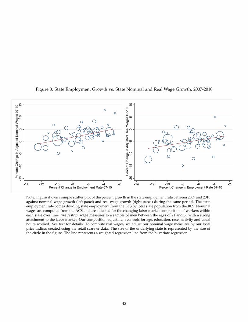
Figure 3: State Employment Growth vs. State Nominal and Real Wage Growth, 2007-2010

-15

-10

-50

510

15P

erce

nt C

hang

e in

Adj

uste

d N

omin

al W

ages

07-

10

-14 -12 -10 -8 -6 -4 -2 0Percent Change in Employment Rate 07-10

-20

-15

-10

-50

510

Per

cent

Cha

nge

in A

djus

ted

Rea

l Wag

es 0

7-10

-14 -12 -10 -8 -6 -4 -2 0Percent Change in Employment Rate 07-10

Note: Figure shows a simple scatter plot of the percent growth in the state employment rate between 2007 and 2010against nominal wage growth (left panel) and real wage growth (right panel) during the same period. The stateemployment rate comes dividing state employment from the BLS by total state population from the BLS. Nominalwages are computed from the ACS and are adjusted for the changing labor market composition of workers withineach state over time. We restrict wage measures to a sample of men between the ages of 21 and 55 with a strongattachment to the labor market. Our composition adjustment controls for age, education, race, nativity and usualhours worked. See text for details. To compute real wages, we adjust our nominal wage measures by our localprice indices created using the retail scanner data. The size of the underlying state is represented by the size ofthe circle in the figure. The line represents a weighted regression line from the bi-variate regression.

42

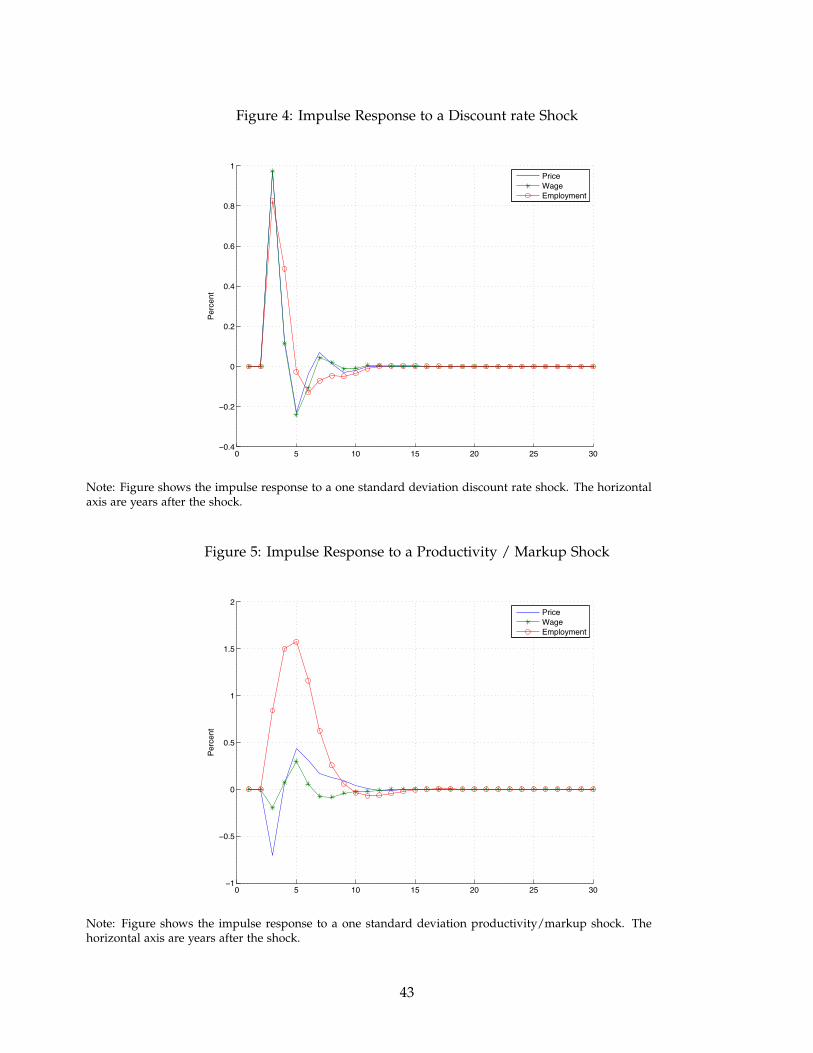
Figure 4: Impulse Response to a Discount rate Shock

0 5 10 15 20 25 30−0.4

−0.2

0

0.2

0.4

0.6

0.8

1

Perc

ent

PriceWageEmployment

Note: Figure shows the impulse response to a one standard deviation discount rate shock. The horizontalaxis are years after the shock.

Figure 5: Impulse Response to a Productivity / Markup Shock

0 5 10 15 20 25 30−1

−0.5

0

0.5

1

1.5

2

Perc

ent

PriceWageEmployment

Note: Figure shows the impulse response to a one standard deviation productivity/markup shock. Thehorizontal axis are years after the shock.

43

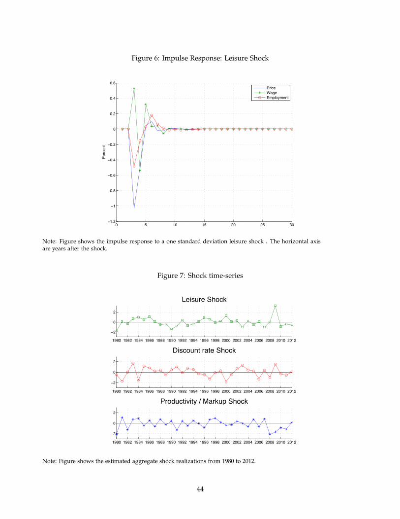
Figure 6: Impulse Response: Leisure Shock

0 5 10 15 20 25 30−1.2

−1

−0.8

−0.6

−0.4

−0.2

0

0.2

0.4

0.6

Perc

ent

PriceWageEmployment

Note: Figure shows the impulse response to a one standard deviation leisure shock . The horizontal axisare years after the shock.

Figure 7: Shock time-series

1980 1982 1984 1986 1988 1990 1992 1994 1996 1998 2000 2002 2004 2006 2008 2010 2012

−2

0

2

Leisure Shock

1980 1982 1984 1986 1988 1990 1992 1994 1996 1998 2000 2002 2004 2006 2008 2010 2012

−2

0

2

Discount rate Shock

1980 1982 1984 1986 1988 1990 1992 1994 1996 1998 2000 2002 2004 2006 2008 2010 2012

−2

0

2

Productivity / Markup Shock

Note: Figure shows the estimated aggregate shock realizations from 1980 to 2012.

44

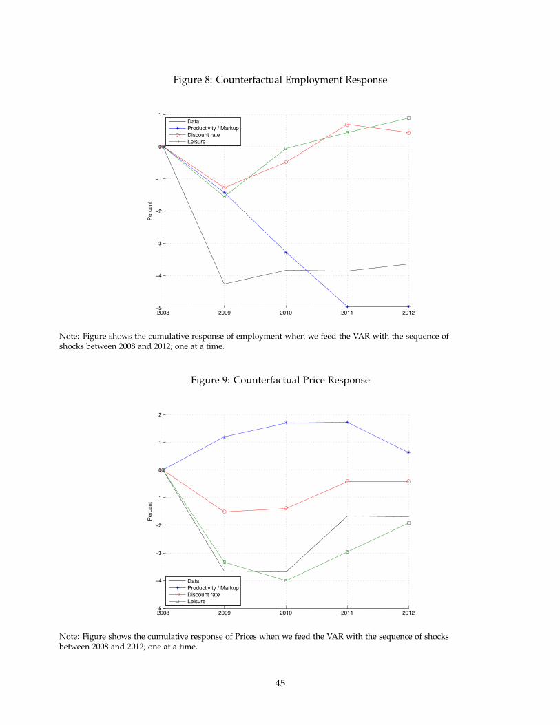
Figure 8: Counterfactual Employment Response

2008 2009 2010 2011 2012−5

−4

−3

−2

−1

0

1

Perc

ent

DataProductivity / MarkupDiscount rateLeisure

Note: Figure shows the cumulative response of employment when we feed the VAR with the sequence ofshocks between 2008 and 2012; one at a time.

Figure 9: Counterfactual Price Response

2008 2009 2010 2011 2012−5

−4

−3

−2

−1

0

1

2

Perc

ent

DataProductivity / MarkupDiscount rateLeisure

Note: Figure shows the cumulative response of Prices when we feed the VAR with the sequence of shocksbetween 2008 and 2012; one at a time.

45

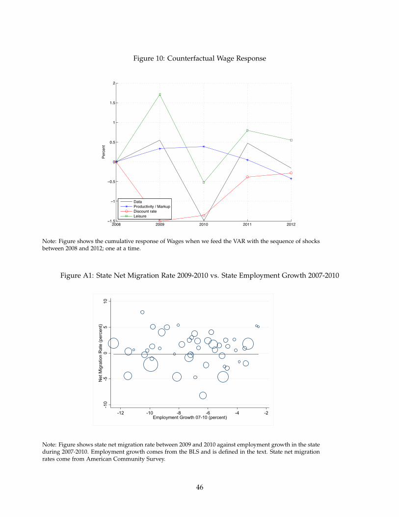
Figure 10: Counterfactual Wage Response

2008 2009 2010 2011 2012−1.5

−1

−0.5

0

0.5

1

1.5

2

Perc

ent

DataProductivity / MarkupDiscount rateLeisure

Note: Figure shows the cumulative response of Wages when we feed the VAR with the sequence of shocksbetween 2008 and 2012; one at a time.

Figure A1: State Net Migration Rate 2009-2010 vs. State Employment Growth 2007-2010

-10

-50

510

Net

Mig

ratio

n R

ate

(per

cent

)

-12 -10 -8 -6 -4 -2Employment Growth 07-10 (percent)

Note: Figure shows state net migration rate between 2009 and 2010 against employment growth in the stateduring 2007-2010. Employment growth comes from the BLS and is defined in the text. State net migrationrates come from American Community Survey.

46

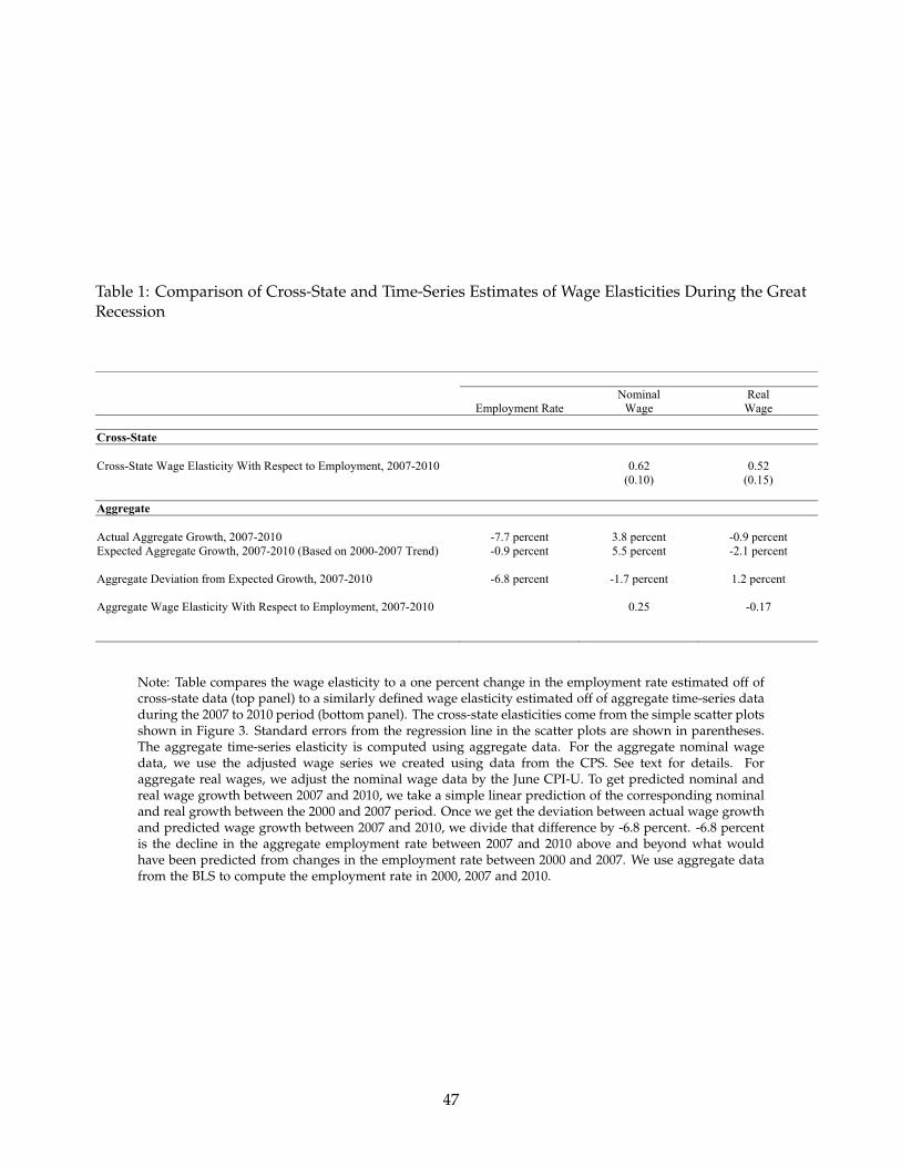
Table 1: Comparison of Cross-State and Time-Series Estimates of Wage Elasticities During the GreatRecession

Employment Rate Nominal

Wage Real

Wage Cross-State Cross-State Wage Elasticity With Respect to Employment, 2007-2010 0.62 0.52 (0.10) (0.15) Aggregate Actual Aggregate Growth, 2007-2010 -7.7 percent 3.8 percent -0.9 percent Expected Aggregate Growth, 2007-2010 (Based on 2000-2007 Trend) -0.9 percent 5.5 percent -2.1 percent Aggregate Deviation from Expected Growth, 2007-2010 -6.8 percent -1.7 percent 1.2 percent Aggregate Wage Elasticity With Respect to Employment, 2007-2010 0.25 -0.17

Note: Table compares the wage elasticity to a one percent change in the employment rate estimated off ofcross-state data (top panel) to a similarly defined wage elasticity estimated off of aggregate time-series dataduring the 2007 to 2010 period (bottom panel). The cross-state elasticities come from the simple scatter plotsshown in Figure 3. Standard errors from the regression line in the scatter plots are shown in parentheses.The aggregate time-series elasticity is computed using aggregate data. For the aggregate nominal wagedata, we use the adjusted wage series we created using data from the CPS. See text for details. Foraggregate real wages, we adjust the nominal wage data by the June CPI-U. To get predicted nominal andreal wage growth between 2007 and 2010, we take a simple linear prediction of the corresponding nominaland real growth between the 2000 and 2007 period. Once we get the deviation between actual wage growthand predicted wage growth between 2007 and 2010, we divide that difference by -6.8 percent. -6.8 percentis the decline in the aggregate employment rate between 2007 and 2010 above and beyond what wouldhave been predicted from changes in the employment rate between 2000 and 2007. We use aggregate datafrom the BLS to compute the employment rate in 2000, 2007 and 2010.

47

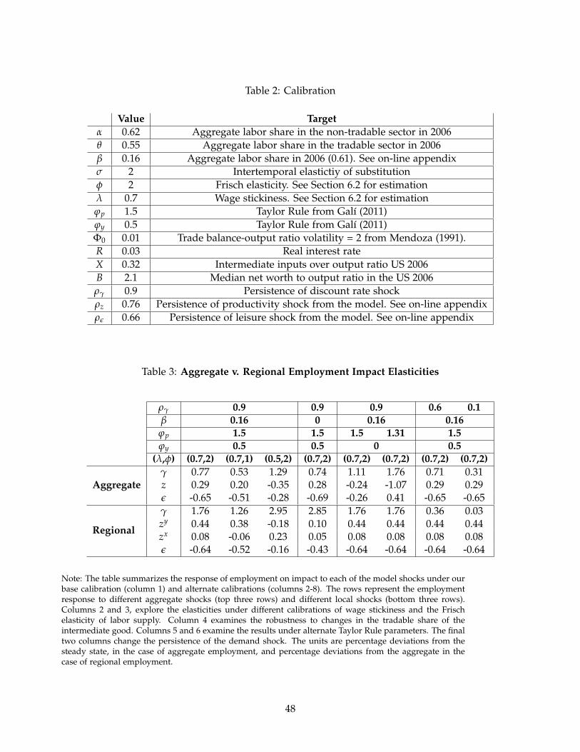
Table 2: Calibration

Value Targetα 0.62 Aggregate labor share in the non-tradable sector in 2006θ 0.55 Aggregate labor share in the tradable sector in 2006β 0.16 Aggregate labor share in 2006 (0.61). See on-line appendixσ 2 Intertemporal elastictiy of substitutionφ 2 Frisch elasticity. See Section 6.2 for estimationλ 0.7 Wage stickiness. See Section 6.2 for estimationϕp 1.5 Taylor Rule from Galí (2011)ϕy 0.5 Taylor Rule from Galí (2011)Φ0 0.01 Trade balance-output ratio volatility = 2 from Mendoza (1991).R 0.03 Real interest rateX 0.32 Intermediate inputs over output ratio US 2006B 2.1 Median net worth to output ratio in the US 2006ργ 0.9 Persistence of discount rate shockρz 0.76 Persistence of productivity shock from the model. See on-line appendixρε 0.66 Persistence of leisure shock from the model. See on-line appendix

Table 3: Aggregate v. Regional Employment Impact Elasticities

ργ 0.9 0.9 0.9 0.6 0.1β 0.16 0 0.16 0.16ϕp 1.5 1.5 1.5 1.31 1.5ϕy 0.5 0.5 0 0.5

(λ,φ) (0.7,2) (0.7,1) (0.5,2) (0.7,2) (0.7,2) (0.7,2) (0.7,2) (0.7,2)γ 0.77 0.53 1.29 0.74 1.11 1.76 0.71 0.31

Aggregate z 0.29 0.20 -0.35 0.28 -0.24 -1.07 0.29 0.29ε -0.65 -0.51 -0.28 -0.69 -0.26 0.41 -0.65 -0.65

Regional

γ 1.76 1.26 2.95 2.85 1.76 1.76 0.36 0.03zy 0.44 0.38 -0.18 0.10 0.44 0.44 0.44 0.44zx 0.08 -0.06 0.23 0.05 0.08 0.08 0.08 0.08ε -0.64 -0.52 -0.16 -0.43 -0.64 -0.64 -0.64 -0.64

Note: The table summarizes the response of employment on impact to each of the model shocks under ourbase calibration (column 1) and alternate calibrations (columns 2-8). The rows represent the employmentresponse to different aggregate shocks (top three rows) and different local shocks (bottom three rows).Columns 2 and 3, explore the elasticities under different calibrations of wage stickiness and the Frischelasticity of labor supply. Column 4 examines the robustness to changes in the tradable share of theintermediate good. Columns 5 and 6 examine the results under alternate Taylor Rule parameters. The finaltwo columns change the persistence of the demand shock. The units are percentage deviations from thesteady state, in the case of aggregate employment, and percentage deviations from the aggregate in thecase of regional employment.

48

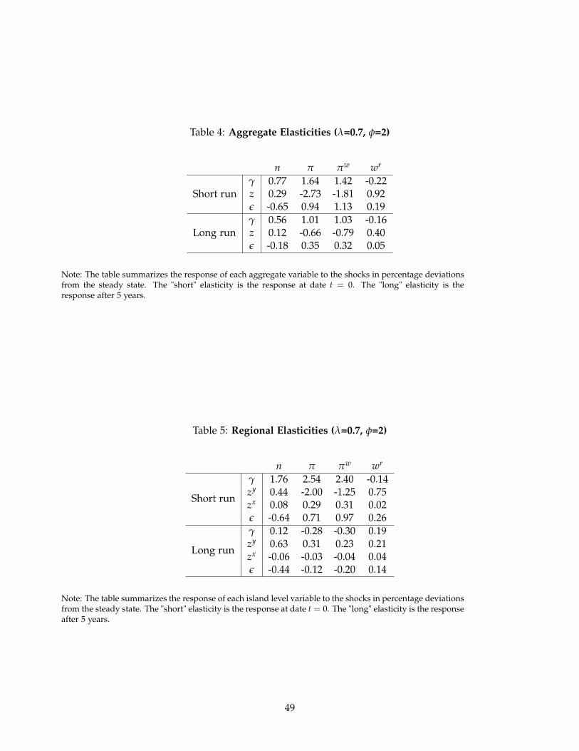
Table 4: Aggregate Elasticities (λ=0.7, φ=2)

n π πw wr

γ 0.77 1.64 1.42 -0.22Short run z 0.29 -2.73 -1.81 0.92

ε -0.65 0.94 1.13 0.19γ 0.56 1.01 1.03 -0.16

Long run z 0.12 -0.66 -0.79 0.40ε -0.18 0.35 0.32 0.05

Note: The table summarizes the response of each aggregate variable to the shocks in percentage deviationsfrom the steady state. The "short" elasticity is the response at date t = 0. The "long" elasticity is theresponse after 5 years.

Table 5: Regional Elasticities (λ=0.7, φ=2)

n π πw wr

Short run

γ 1.76 2.54 2.40 -0.14zy 0.44 -2.00 -1.25 0.75zx 0.08 0.29 0.31 0.02ε -0.64 0.71 0.97 0.26

Long run

γ 0.12 -0.28 -0.30 0.19zy 0.63 0.31 0.23 0.21zx -0.06 -0.03 -0.04 0.04ε -0.44 -0.12 -0.20 0.14

Note: The table summarizes the response of each island level variable to the shocks in percentage deviationsfrom the steady state. The "short" elasticity is the response at date t = 0. The "long" elasticity is the responseafter 5 years.

49

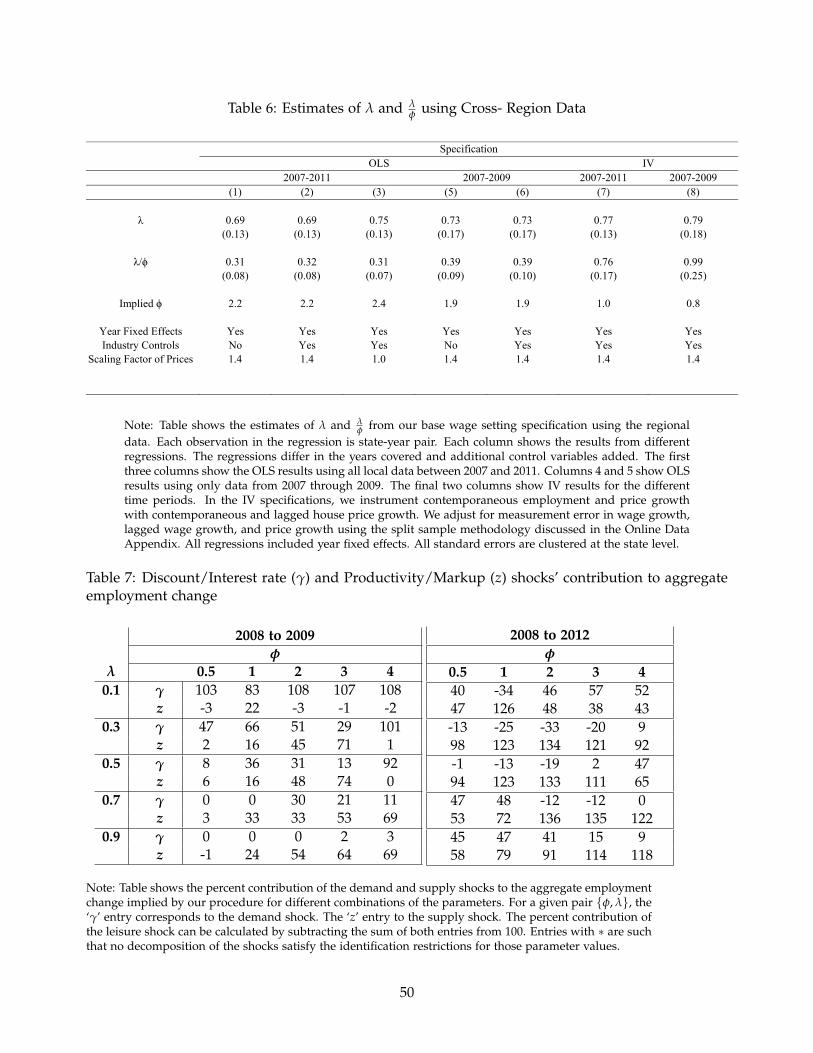
Table 6: Estimates of λ and λφ using Cross- Region Data

Specification OLS IV 2007-2011 2007-2009 2007-2011 2007-2009 (1) (2) (3) (5) (6) (7) (8) λ 0.69 0.69 0.75 0.73 0.73 0.77 0.79 (0.13) (0.13) (0.13) (0.17) (0.17) (0.13) (0.18)

λ/ϕ 0.31 0.32 0.31 0.39 0.39 0.76 0.99 (0.08) (0.08) (0.07) (0.09) (0.10) (0.17) (0.25)

Implied ϕ 2.2 2.2 2.4 1.9 1.9 1.0 0.8

Year Fixed Effects Yes Yes Yes Yes Yes Yes Yes Industry Controls No Yes Yes No Yes Yes Yes

Scaling Factor of Prices 1.4 1.4 1.0 1.4 1.4 1.4 1.4

Note: Table shows the estimates of λ and λ

φ from our base wage setting specification using the regionaldata. Each observation in the regression is state-year pair. Each column shows the results from differentregressions. The regressions differ in the years covered and additional control variables added. The firstthree columns show the OLS results using all local data between 2007 and 2011. Columns 4 and 5 show OLSresults using only data from 2007 through 2009. The final two columns show IV results for the differenttime periods. In the IV specifications, we instrument contemporaneous employment and price growthwith contemporaneous and lagged house price growth. We adjust for measurement error in wage growth,lagged wage growth, and price growth using the split sample methodology discussed in the Online DataAppendix. All regressions included year fixed effects. All standard errors are clustered at the state level.

Table 7: Discount/Interest rate (γ) and Productivity/Markup (z) shocks’ contribution to aggregateemployment change

2008 to 2009φ

λ 0.5 1 2 3 40.1 γ 103 83 108 107 108

z -3 22 -3 -1 -20.3 γ 47 66 51 29 101

z 2 16 45 71 10.5 γ 8 36 31 13 92

z 6 16 48 74 00.7 γ 0 0 30 21 11

z 3 33 33 53 690.9 γ 0 0 0 2 3

z -1 24 54 64 69

2008 to 2012φ

0.5 1 2 3 440 -34 46 57 5247 126 48 38 43-13 -25 -33 -20 998 123 134 121 92-1 -13 -19 2 4794 123 133 111 6547 48 -12 -12 053 72 136 135 12245 47 41 15 958 79 91 114 118

Note: Table shows the percent contribution of the demand and supply shocks to the aggregate employmentchange implied by our procedure for different combinations of the parameters. For a given pair {φ, λ}, the‘γ’ entry corresponds to the demand shock. The ‘z’ entry to the supply shock. The percent contribution ofthe leisure shock can be calculated by subtracting the sum of both entries from 100. Entries with ∗ are suchthat no decomposition of the shocks satisfy the identification restrictions for those parameter values.

50