THE AERODYNAMIC EXCITATION OF TRAPPED DIAMETRAL …
136
THE AERODYNAMIC EXCITATION OF TRAPPED DIAMETRAL ACOUSTIC MODES IN RECTANGULAR DUCTED CAVITIES
Transcript of THE AERODYNAMIC EXCITATION OF TRAPPED DIAMETRAL …

THE AERODYNAMIC EXCITATION OF
TRAPPED DIAMETRAL ACOUSTIC
MODES IN RECTANGULAR DUCTED
CAVITIES

The Aerodynamic Excitation of Trapped Diametral
Acoustic Modes in Rectangular Ducted Cavities
By
MICHAEL BOLDUC, B.ENG & MGT
A Thesis
Submitted to the School of Graduate Studies
In Partial Fulfillment of the Requirements
For the Degree
Master of Applied Science
McMaster University
©Copyright Michael Bolduc, September 2015

ii
Master of Applied Science (2015) McMaster University
Mechanical Engineering Hamilton, Ontario, Canada
TITLE: The Aerodynamic Excitation of Trapped Diametral
Acoustic Modes in Rectangular Ducted Cavities
AUTHOR: Michael Bolduc, B.Eng&Mgt. (McMaster University)
SUPERVISORS: Professor Samir Ziada
NUMBER OF PAGES: xvii, 118

iii
Abstract
The excitation mechanism of trapped diametral acoustic modes within a
rectangular cavity-duct system is investigated both numerically and
experimentally. The asymmetry inherent within the rectangular geometry
introduces a preferred orientation, ensuring the excited diametral modes remain
stationary. Three separate cavities are manufactured and tested. This included two
asymmetric rectangular cross-sections and one symmetric square cavity.
Experimental results indicate that the aeroacoustic responses of the three cavities
are dominated by the strong excitation of trapped diametral modes. Numerical
simulations indicate that the resolved radial acoustic particle velocity distributions
are non-uniform at the upstream separation edge where the formation of vortical
structures is initiated. As the cavity became smaller, and more asymmetric, the
trapped nature of the acoustic modes decreased with an accompanied increase in
the radiation losses and reduction in pulsation amplitude.
Observations of the aeroacoustic measurements show evidence of three unique
modal behaviours. The first case is the independent excitation of a single
stationary mode where specific circumferential sections of the shear layer were
excited and initiating the formation of vortical disturbances. These circumferential
sections, and distribution of disturbances, were akin to the excited mode shape.
The second case involved simultaneous excitation of two stationary modes. This
suggested that the shear layer was exciting two modes simultaneously.
Neighbouring circumferential sections, at the initial region of the shear layer,
were being excited independently and at different resonant frequencies. Finally, a
spinning trapped acoustic mode was observed in the symmetric square cavity.
Due to the spinning nature, the excited circumferential portions and formation of
vortices were non-uniform and rotated with the spinning acoustic mode. This
resulted in the formation of a three-dimensional helical structure.

iv
ACKNOWLEDGEMENTS
I would first like to thank my supervisor Dr. Samir Ziada for his guidance
throughout the years. I remain entirely grateful for his advice and encouragement
that has proved invaluable both within this study and within my educational
career. For this I remain forever in his debt.
I would like to also extend my gratitude to Philippe Lafon for his additional
counsel and suggestions within this current study. As well, I would like to thank
all of my colleagues within the Flow Induced Vibration group at McMaster
University, past and present, who would always lend a hand when in need.
Through their expertise and help in building the experimental test set-up, I extend
my gratitude to the technicians within the Mechanical Engineering Department,
particularly Michael Lee, John Colenbrander, Mark MacKenzie, Joe Verhaeghe,
and Ron Lodewyks.
Last but not least I would like to thank my family and friends, especially
Victoria Tran, for their continuous support and motivation which allowed me to
overcome the challenges that I encountered throughout these past few years.

v
NOMENCLATURE
c Speed of sound [m/s]
d Diameter of jet [m]
D Pipe diameter [m]
f Frequency [Hz]
f1 Resonant frequency of trapped acoustic mode 1 [Hz]
f2 Resonant frequency of trapped acoustic mode 2 [Hz]
f3 Resonant frequency of trapped acoustic mode 3 [Hz]
f4 Resonant frequency of trapped acoustic mode 4 [Hz]
h Cavity depth [m]
H Cavity cross-sectional height [m]
K Adiabatic bulk modulus [Pa]
L Cavity length [m]
Pipe length [m]
m Diametral mode number for axisymmetric cavity []
M Mach number []
n Free shear layer mode number []
P Acoustic pressure [Pa]
P Acoustic power production [W]
Density [kg/ ]
Pressure gradient [Pa]
Dimensionless acoustic pressure []
Reynolds number based on momentum thickness []
Reynolds number based on pipe diameter []
Strouhal number based on momentum thickness []
SPL Sound pressure level ref: 20uPa [dB]
Strouhal Number based on cavity length []

vi
t Time [s]
Jet centerline velocity [m/s]
Mean flow velocity vector [m/s]
Acoustic particle velocity vector [m/s]
Radial acoustic particle velocity [m/s]
V(z) Velocity variation along shear layer [m/s]
W Cavity cross-sectional width [m]
x Axial distance [m]
y Downstream position from upstream corner [m]
Momentum thickness [m]
Phase along the acoustic cycle of spinning mode [deg]
Physical angle along the upstream cavity mouth [deg]
ϕ PIV temporal phase shifts along acoustic cycle [deg]
Vorticity vector [1/s]
Angular resonance frequency [rad/s]
Volume [

vii
TABLE OF CONTENTS
ABSTRACT........................................................................................................... iii
ACKNOWLEDGEMENTS..................................................................................iv
NOMENCLATURE............................................................................................... v
CHAPTER 1: Introduction................................................................................... 1
1.1 Problem and Motivation........................................................................... 1
1.2 Thesis Outline........................................................................................... 3
CHAPTER 2: Literature Review......................................................................... 5
2.1 Introduction...............................................................................................5
2.2 The Instability of Free Shear Layers........................................................ 6
2.3 Classification of Feedback Mechanisms................................................ 10
2.4 Acoustic Modes of Self-Sustaining Cavity Oscillations........................ 13
2.4.1 Trapped Acoustic Modes........................................................... 14
2.4.2 Axisymmetric Cavities............................................................... 16
2.5 Fluid-Resonant Excitation Mechanism.................................................. 20
2.5.1 Hydrodynamic Modes or Free Shear Layer Modes................... 22
2.5.2 Distribution of Acoustic Particle Velocity................................. 23
2.6 Effects of Symmetry on the Diametral Modes....................................... 25
2.7 Noise Control of Trapped Diametral Modes.......................................... 31
2.8 Objectives............................................................................................... 33
CHAPTER 3: Experimental Apparatus............................................................ 35
3.1 Test Facility............................................................................................ 35
3.2 Test Setup............................................................................................... 37
3.2.1 Cavity Geometry........................................................................ 38
3.2.2 Test Section Assembly............................................................... 40
3.3 Numerical Simulations........................................................................... 42
3.3.1 Simulation and Mesh Configuration.......................................... 42
3.3.2 Simulated Trapped Diametral Acoustic Modes......................... 44

viii
3.4 Acoustic Particle Velocity...................................................................... 48
3.4.1 Radial Acoustic Particle Velocity Distributions........................ 50
3.4.2 Effect of Geometry.................................................................... 52
3.5 Instrumentation....................................................................................... 55
3.5.1 Dynamic Pressure Transducers.................................................. 55
3.5.2 Pitot-tube.................................................................................... 56
3.5.3 Laser Doppler Velocimetry (LDV)........................................... 56
3.5.4 Particle Image Velocimetry (PIV)............................................. 57
CHAPTER 4: Results and Discussion................................................................ 61
4.1 Introduction............................................................................................ 61
4.2 Aeroacoustic Measurements................................................................... 62
4.2.1 Measurement Procedure............................................................. 62
4.2.2 General Behaviour of the Trapped Diametral Modes................ 65
4.2.3 Effect of Geometry on Aeroacoustic Measurements................. 69
4.2.4 Effect on Pressure Drop............................................................. 73
4.3 Upstream Flow Conditions..................................................................... 74
4.4 Modal Behaviours.................................................................................. 75
4.4.1 Excitation of a Single Stationary Trapped Diametral Mode...... 76
4.4.2 Simultaneous Excitation of Two Separate Modes..................... 82
4.4.3 Simultaneous Excitation of Two Degenerate Modes................. 90
CHAPTER 5: Conclusions.................................................................................. 99
5.1 Summary................................................................................................. 99
5.2 Suggestions for Future Work............................................................... 101
REFERENCES................................................................................................... 102
APPENDIX......................................................................................................... 107
A: Additional Results............................................................................. 107
B: Uncertainty Analysis......................................................................... 115

ix
LIST OF FIGURES
Figure 1-1 Schematic of PWR plant and its isolation gate valves situated
along the main piping (Lacombe et al., 2013)................................. 1
Figure 2-1 Development and breakdown of disturbances within a free shear
layer (Chevray, 1984)....................................................................... 6
Figure 2-2 Hyperbolic-tangent velocity profile utilized by Michalke (1964,
1965) reminiscent of an unstable free shear layer within grazing
cavity flows...................................................................................... 7
Figure 2-3 Effect of acoustic pressure on the downstream growth of velocity
fluctuations from an axisymmetric jet, ○=70dB, ●=80dB, ∆=90dB,
X=100dB, d=7.5cm, U0=8.0m/s, R =122, St =0.0118
(Freymuth,1966)............................................................................... 8
Figure 2-4 Effect of Strouhal Number on the downstream growth of transverse
fluctuations of an axisymmetric jet, ⌛, =0.0020, ⊗,
=0.0040, ●, =0.0050, ✳, =0.0070, ∆, =0.0080,
○, =0.0090, X, =0.0100,□, =0.0118, ▲,
=0.0148, ●, =0.0176, ■, =0.0234 d=7.5cm,
U0=16.0m/s(Freymuth, 1966).......................................................... 9
Figure 2-5 Comparison of numerical and experimental growth rates as a
function of for axisymmetric,○, and planar, X, free jets
(Freymuth, 1966).............................................................................. 9
Figure 2-6 Flowchart illustrating the general sequence of events within
self-sustained cavity oscillations.................................................... 11
Figure 2-7 Common cavity oscillations categorized into the fluid-dynamic,
fluid-resonant and fluid-elastic feedback mechanisms
(Rockwell & Naudascher, 1978).................................................... 13
Figure 2-8 Schematic of axisymmetric cavity-duct domain with corresponding
dimensions..................................................................................... 16
Figure 2-9 Trapped acoustic mode shapes for the first three diametral modes
for the L/h=1, h=25.4mm, axisymmetric cavity (Aly & Ziada,
2010). The dotted lines represent the nodal lines........................... 17

x
Figure 2-10 Exponential decrease in acoustic pressure of the first diametral
mode with axial distance from the cavity domain for varying
depths, h, for axisymmetric cavities (Aly & Ziada, 2010)............. 18
Figure 2-11 Waterfall SPL contour plot detailing the aeroacoustic response of
the trapped diametral modes for the h=12.7mm, L/h=2
axisymmetric cavity (Aly & Ziada, 2010)..................................... 19
Figure 2-12 Waterfall SPL contour plot detailing the aeroacoustic response of
the trapped diametral modes for the h=50.8mm, L/h=0.5
axisymmetric cavity (Aly & Ziada, 2010)..................................... 19
Figure 2-13 Illustration detailing the energy exchange between the flow field
and the resonant sound field during an acoustic cycle of a
transverse acoustic mode in a deep cavity (Ziada, 2010)............... 21
Figure 2-14 Relationship of dimensionless acoustic pressure and Strouhal
number during the excitation of the three diametral trapped
acoustic modes, h=50.8mm, L/h=0.5 axisymmetric cavity (Aly &
Ziada,2010).................................................................................... 23
Figure 2-15 Radial acoustic particle velocity distribution of the diametral
modes within an axisymmetric cavity with h=25.4mm, L/h=1 (Aly
& Ziada, 2010)............................................................................... 24
Figure 2-16 Schematic of two equivalent orthogonal modes with amplitudes
A & B............................................................................................. 27
Figure 2-17 Comparison of the fully spinning, A/B=1, (left) and partially
spinning, A/B=0.4, (right) acoustic modes within an axisymmetric
cavity along six equal interval phases of its half acoustic cycle
(Aly, 2008)..................................................................................... 27
Figure 2-18 Two resolved equivalent orthogonal modes whose resonant
frequency, f=1198Hz, was detected through turbulent fluctuations
(Selle et al.,2006)........................................................................... 28
Figure 2-19 Cross-sectional view used in the visualization of the acoustic
spinning mode (Selle et al.,2006)................................................... 29
Figure 2-20 Simulated mode shape (left), axial acoustic particle velocity
(middle), and helical vortex (right) during half an acoustic cycle of
the spinning acoustic mode (Selle et al.,2006)............................... 30

xi
Figure 2-21 Schematic of geometric modifications at the upstream cavity edge.
From left to right, sharp edge, rounding, chamfering, and saw-tooth
spoiler (Bolduc et al., 2014)........................................................... 32
Figure 2-22 Photograph illustrating upstream geometric modifications of the
curved and delta spoilers (Bolduc et al., 2014).............................. 32
Figure 3-1 Schematic of Test Facility and its components.............................. 36
Figure 3-2 Schematic of Test Setup (Aly & Ziada, 2010)............................... 37
Figure 3-3 Schematic of cavity dimensions and geometry.............................. 38
Figure 3-4 Dimensional comparisons between axisymmetric and present
square cavity (dashed).................................................................... 39
Figure 3-5 Dimensionless aeroacoustic pressure response for axisymmetric
cavity, L/h=0.5, h/D=1/3 (Aly & Ziada, 2010).............................. 39
Figure 3-6 Detailed exploded assembly of test section.................................... 40
Figure 3-7 Dimensions (mm) of Constant side wall used in all three
cavities............................................................................................ 41
Figure 3-8 Dimensions (mm) of Variable top and bottom walls with varying
dimension X................................................................................... 41
Figure 3-9 Influence of pipe length per diameter ( /D) on simulated resonant
frequency, W/H=0.9, first acoustic mode....................................... 43
Figure 3-10 Convergence of first resonant frequency with increasing number of
elements, W/H=0.9 rectangular cavity........................................... 44
Figure 3-11 Resolved mode shapes of the four trapped acoustic modes at the
center of the rectangular, W/H=0.9, cavity.....................................45
Figure 3-12 Simplified schematic of a uniform radial acoustic particle velocity
vector distribution, , represented by dashed vectors. This
initiates the formation of disturbances at the upstream
axisymmetric separation edge........................................................ 48

xii
Figure 3-13 Dimensionless (Top Left) Acoustic pressure distribution, (Top
Right) Acoustic particle velocity magnitude, (Bottom Left) Radial
acoustic particle velocity distribution, (Bottom Right) Radial
particle velocity along shear layer circumference (all figures
correspond to 0.2mm downstream from the inlet of the W/H=0.9
rectangular cavity).......................................................................... 50
Figure 3-14 Normalized acoustic pressure distribution and corresponding radial
acoustic particle velocity along the upstream cavity mouth for the
W/H=0.9 rectangular cavity............................................................51
Figure 3-15 Dimensionless Acoustic Particle velocity distributions of the four
acoustic modes for the rectangular, W/H=0.9, cavity. All cases
correspond to the upstream cavity corner...................................... 52
Figure 3-16 Comparison of dimensionless radial particle velocity distribution
for the second acoustic mode as a function of angle, , along the
upstream cavity corner of the three cavity geometries.................. 53
Figure 3-17 Comparison of dimensionless radial particle velocity distribution
for the third acoustic mode as a function of angle, , along the
upstream cavity corner of the three cavity geometries.................. 53
Figure 3-18 Comparison of dimensionless radial particle velocity distribution
for the fourth acoustic mode as a function of angle, , along the
upstream cavity corner of the three cavity geometries.................. 54
Figure 3-19 Location of four installed dynamic pressure transducers (PT1-4) in
comparison to the four simulated mode shapes............................. 55
Figure 3-20 Schematic illustrating the two orthogonal measurement planes
denoted by views A-A and B-B..................................................... 58
Figure 3-21 Isometric model illustrating the PIV test setup and A-A
measurement plane........................................................................ 58
Figure 4-1 Acoustic pressure spectra of each of the four dynamic pressure
transducers for the rectangular W/H=0.9 cavity, 83m/s................. 62
Figure 4-2 SPL contour plot of the aeroacoustic response for the rectangular,
W/H=0.9, cavity............................................................................. 63
Figure 4-3 Aeroacoustic response of the W/H=0.9 cavity, detailing pulsation
amplitudes of each of the four dominant trapped acoustic modes. 65

xiii
Figure 4-4 Associated resonant frequencies corresponding to the above
dominant pressure pulsations, indicating jumps in resonant
frequency with increase in flow velocity....................................... 65
Figure 4-5 Strouhal number as a function of the mean flow velocity during the
dominant excitation of the four trapped acoustic modes of the
cavity with W/H=0.9...................................................................... 67
Figure 4-6 Dimensionless acoustic pressure of the dominant acoustic modes as
a function of the Strouhal number for the W/H=0.9,
cavity.............................................................................................. 67
Figure 4-7 Dimensionless acoustic pressure of the dominant acoustic modes as
a function of the Strouhal number for the square,
W/H=1, cavity................................................................................. 68
Figure 4-8 Aeroacoustic response detailing the excitation of each of the
trapped modes for the rectangular, W/H=0.95, cavity....................70
Figure 4-9 Aeroacoustic response detailing the excitation of each of the
trapped modes for the rectangular, W/H=0.9, cavity......................70
Figure 4-10 Dimensionless pressure signals indicating beating within the corner
pressure transducers, W/H=0.9 cavity, 31m/s................................ 71
Figure 4-11 Aeroacoustic response detailing the excitation of each of the
trapped modes for the square, W/H=1, cavity................................ 72
Figure 4-12 Static pressure drop across the square, W/H=1.0, cavity during its
aeroacoustic response..................................................................... 73
Figure 4-13 Radial profile of mean flow velocity measured one pipe diameter
upstream of square cavity at pre-resonance conditions, 36.5m/s... 74
Figure 4-14 Radial profile of mean flow velocity measured one pipe diameter
upstream of square cavity at resonance conditions, 61m/s............ 74
Figure 4-15 Normalized acoustic pressure and radial acoustic particle velocity
distribution of the fourth acoustic mode at the cavity corner,
W/H=1, square cavity..................................................................... 76

xiv
Figure 4-16 Schematic illustrating the four projected measurement domains and
their respective field-of-view for PIV flow visualization. Phase-
averaging through all tests was done through triggering pressure
transducers PT2 and PT3................................................................77
Figure 4-17 Phase-averaged vorticity fields during the excitation of the fourth
acoustic mode for four instants during the acoustic cycle separated
by 90˚ phase shifts, ϕ, f4=1480Hz, 104m/s.................................... 78
Figure 4-18 Normalized acoustic pressure and radial acoustic particle velocity
distribution of the third acoustic mode at the upstream cavity
corner, W/H=1, square cavity......................................................... 79
Figure 4-19 Phase-averaged vorticity fields during the excitation of the third
acoustic mode for four instants during the acoustic cycle separated
by 90˚ phase shifts, ϕ, f3=1027Hz, 81m/s...................................... 80
Figure 4-20 Acoustic spectra of pressure transducer PT2 and PT3 during the
excitation of the third acoustic mode, 81m/s..................................81
Figure 4-21 Time averaged acoustic spectra of the four pressure transducers
during simultaneous excitation of the third and fourth acoustic
mode for the square cavity at 92m/s...............................................82
Figure 4-22 Instantaneous time signal of PT 2, depicting sinusoidal oscillations
at f4=1480Hz.................................................................................. 83
Figure 4-23 Instantaneous time signal of PT 3, depicting sinusoidal oscillations
at f3=1033Hz.................................................................................. 83
Figure 4-24 Dimensionless acoustic pressure and radial acoustic particle
velocity distributions for the simultaneous excitation of the third
and fourth acoustic mode............................................................... 85
Figure 4-25 Phase-averaged vorticity fields during dual excitation
corresponding to the fourth acoustic mode taken at four instants of
the fourth mode acoustic cycle separated by 90˚ phase shifts, ϕ,
f4=1484Hz, 91m/s......................................................................... 86
Figure 4-26 Phase-averaged vorticity fields during dual excitation
corresponding to the third acoustic mode taken at four instants of
the third mode acoustic cycle separate by 90˚ phase shifts, ϕ,
f3=1033Hz, 91m/s.......................................................................... 87

xv
Figure 4-27 Instantaneous vorticity field through phase-triggering long the third
mode’s acoustic cycle illustrating a pair of vortices from the
simultaneous excitation of the fourth mode................................... 88
Figure 4-28 Acoustic mode shapes and radial particle velocity distributions of
the first two acoustic modes, W/H=0.9 cavity................................ 89
Figure 4-29 Instantaneous time signals illustrating the spinning behaviour of the
degenerate mode for the square cavity, 63m/s............................... 91
Figure 4-30 Super positioned orthogonal modes normalized by largest
amplitude within the acoustic cycle of the
resultant spinning mode.................................................................. 92
Figure 4-31 Instantaneous normalized acoustic pressure contours of spinning
degenerate mode at phase, .......................................................... 94
Figure 4-32 Instantaneous normalized radial acoustic particle velocity contours
of spinning degenerate mode at phase, ....................................... 95
Figure 4-33 Projected measurement domains and spinning direction for the
degenerate acoustic mode...............................................................96
Figure 4-34 Flow visualization of phase-averaged vorticity fields displaying the
helical propagation of disturbances along the four measurement
domains at separate phase angles, ϕ, of the spinning degenerate
mode, 59m/s, 851Hz.......................................................................96
Figure 4-35 Smoke flow visualization of a torodial vortex (left) and helical
vortex (right) from the external excitation of a free round jet
(Kusek et al., 1990)........................................................................ 97
Figure 4-36 Radial acoustic particle velocity distribution of the diametral
modes within an axisymmetric cavity with h=25.4mm, L/h=1 (Aly
& Ziada, 2010)............................................................................... 98
Figure A-1 Comparison of dimensionless radial particle velocity distribution
for the first acoustic mode as a function of angle, ∅, upstream
cavity corner of the three cavity geometries................................ 107
Figure A-2 Dimensionless Acoustic Particle velocity distributions of the four
acoustic modes for the Top: W/H=1, Middle: W/H=0.95, Bottom:
W/H=0.9, cavities........................................................................ 108

xvi
Figure A-3 SPL contour plot of the aeroacoustic response for Top=W/H=1,
Middle=W/H=0.95, Bottom=W/H=0.9 cavities........................... 109
Figure A-4 Frequency [Hz] vs. Mean Flow Velocity [m/s] Top=W/H=1,
Middle=W/H=0.95, Bottom=W/H=0.9 cavities........................... 110
Figure A-5 Strouhal Number vs. Mean Flow Velocity [m/s] Top=W/H=1,
Middle=W/H=0.95, Bottom=W/H=0.9 cavities........................... 111
Figure A-6 Dimensionless Acoustic Pressure vs. Strouhal Number
Top=W/H=1, Middle=W/H=0.95, Bottom=W/H=0.9 cavities..... 112
Figure A-7 Pressure drop for the rectangular cavity with W/H=0.95............. 113
Figure A-8 Pressure drop for the rectangular cavity with W/H=0.90............. 114

xvii
LIST OF TABLES
Table 3-1 Dimensions of three manufactured cavities, L=25.4mm and
H=254mm....................................................................................... 38
Table 3-2 Dimensions (mm) of variable x corresponding to the three separate
manufactured cavities..................................................................... 41
Table 3-3 Simulated resonant frequencies of the four trapped acoustic modes
for the three cavity geometries....................................................... 47
Table 4-1 Comparisons of experimental resonant frequencies to simulated
resonant frequencies for the four trapped modes in the W/H=0.9
rectangular cavity........................................................................... 64
M.A.Sc. Thesis – Michael Bolduc McMaster – Mechanical Engineering
1
CHAPTER 1 INTRODUCTION
1.1 Problem and Motivation
Self-sustained oscillations due to flow over cavities have been studied
extensively within the literature due to large-amplitude pressure pulsations arising
in numerous industrial applications including piping systems, fuselage openings,
control valves, jet engines, turbo-compressors, and rocket engines.
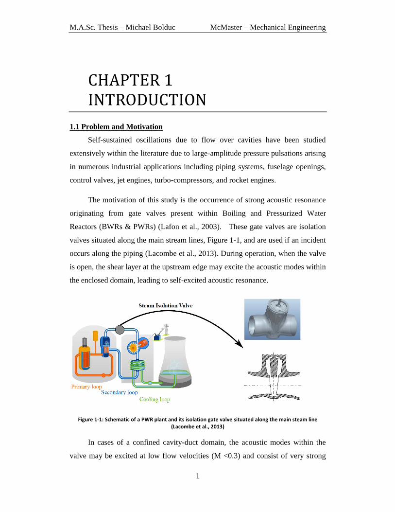
The motivation of this study is the occurrence of strong acoustic resonance
originating from gate valves present within Boiling and Pressurized Water
Reactors (BWRs & PWRs) (Lafon et al., 2003). These gate valves are isolation
valves situated along the main stream lines, Figure 1-1, and are used if an incident
occurs along the piping (Lacombe et al., 2013). During operation, when the valve
is open, the shear layer at the upstream edge may excite the acoustic modes within
the enclosed domain, leading to self-excited acoustic resonance.
Figure 1-1: Schematic of a PWR plant and its isolation gate valve situated along the main steam line (Lacombe et al., 2013)
In cases of a confined cavity-duct domain, the acoustic modes within the
valve may be excited at low flow velocities (M <0.3) and consist of very strong

M.A.Sc. Thesis – Michael Bolduc McMaster – Mechanical Engineering
2
pressure pulsations. These acoustic modes are referred to in the literature as being
“trapped’ as the acoustic energy is confined within the valve geometry with
negligible radiation being emitted down the attached piping (Hein & Koch, 2008;
Aly & Ziada, 2010). The excitation of these trapped acoustic modes can lead to
disastrous results. In the tests conducted within this thesis, amplitude levels of
174dB (ref: 20uPa) were commonly measured at the anti-nodes of the excited
acoustic modes. Within industry, these amplitude levels exceed the limits of noise
regulations and pose a serious safety concern to workers on site (Smith & Luloff,
1999). Also, these strong pressure oscillations may lead to fatigue failure both
within the valve and in nearby piping and supports (Ziada & Bühlmann, 1989;
NRC, 2002).
As well, the pressure drop across the valve increases during acoustic
resonance, an effect demonstrated in the experimental results found in Appendix
A. The kinetic energy from the mean flow is now being used to sustain the strong
acoustic resonance. This leads to undesirable economic effects as it reduces the
overall efficiency of the plant. A BWR power plant consists of numerous steam
lines, each consisting of its own isolation valves. Thus, the excitation of more
than one of these isolation valves in unison is possible, potentially escalating each
of these associated problems.
The general excitation mechanism is due to an interaction between flow
instabilities at the upstream edge and the acoustic mode’s resonant sound field.
The instability of the shear layer causes the disturbances to amplify downstream
into large vortical structures. These structures then impart energy into the resonant
sound field, strengthening the acoustic pressure oscillations. The velocity
fluctuations from the acoustic particle velocity then initiate the formation of larger
disturbances at the upstream edge, closing the feedback cycle.
The excited acoustic modes within the gate valve domain are the transverse
diametral modes. Unlike longitudinal acoustic modes, these mode shapes are

M.A.Sc. Thesis – Michael Bolduc McMaster – Mechanical Engineering
3
three-dimensional within the cavity geometry. This leads to a non-uniform
interaction between the shear layer instability and the acoustic particle velocity.
Previous studies investigating the excitation mechanism of trapped diametral
modes (Aly & Ziada, 2010), their azimuthal behaviour (Aly & Ziada, 2011), the
effect of mean flow (Aly & Ziada, 2012), and passive mitigation techniques
(Bolduc et al., 2014) have focused on axisymmetric cavity-duct geometries.
However, the existence of an asymmetric acoustic mode within an axisymmetric
geometry resulted in the acoustic modes having no unique orientation. As such,
they tended to spin about the pipe’s axis at their resonant frequency.
The cavity geometries for industrial gate valves are generally not
axisymmetric; therefore the diametral acoustic modes are stationary. The present
study considers such a case, where the asymmetry of the rectangular cross-
sectional geometry specifies one unique orientation for each of the excited
diametral acoustic modes. This simplified model allows one to experimentally
investigate the complex three-dimensional interaction between the non-uniform
acoustic particle velocity distribution at the shear layer and its propagation of
vortical structures. As well, the presented experimental results may be used to
validate numerical simulations which are used to predict the aeroacoustic
characteristics of these excited diametral acoustic modes.
1.2 Thesis Layout
This thesis is composed of four separate chapters. Chapter 2 presents a
literature review on the excitation of trapped diametral acoustic modes. First, an
overview of free shear layer instabilities and its interaction with the fluid-resonant
feedback mechanism is covered. An assortment of self-sustaining cavity
oscillations is then investigated before focusing on the current case of trapped
diametral acoustic modes. A review of recent studies on trapped diametral modes
within axisymmetric cavities is presented, including the influence of symmetry
and current mitigation techniques. Finally, the objectives of the current study are
stated.

M.A.Sc. Thesis – Michael Bolduc McMaster – Mechanical Engineering
4
Chapter 3 details the experimental facility and test setup used in
investigating the excitation mechanism of trapped diametral modes within
rectangular cavities. The test-setup consists of three separate cross-sectional
cavities, one which is square while the other two are rectangular. Numerical
simulations of the acoustic mode shapes and their radial acoustic particle velocity
distributions are presented along with the instrumentations used.
Chapter 4 presents the experimental results utilizing the experimental
facility from Chapter 3. The aeroacoustic responses of the trapped acoustic
modes, for each of the three tested cavities, are presented and compared.
Emphasis is then placed on the complex flow-acoustic coupling of three observed
modal behaviours. The analysis consisted of comparing the resolved radial
acoustic particle velocity to the corresponding vortical structures along the
circumference of the shear layer. Qualitative flow visualization of these structures
was done through phase-averaged Particle Image Velocimetry. Finally, Chapter 5
provides a summary of the work along with suggested improvements on current
passive suppression methods.

M.A.Sc. Thesis – Michael Bolduc McMaster – Mechanical Engineering
5
CHAPTER 2 LITERATURE REVIEW
2.1 Introduction
The following chapter presents a literature review on the acoustic resonance
of trapped diametral acoustic modes within cavities. The chapter begins with the
general excitation mechanism of self-sustained cavity oscillations, including the
interaction between the flow instability at the upstream cavity corner, and an
upstream propagating feedback mechanism.
The fluid-resonant feedback mechanism is a result of the acoustic particle
velocity imparting velocity fluctuations at the upstream separation edge of the
cavity, initiating and strengthening disturbances into large vortical structures. This
closes the feedback cycle. Depending on the acoustic mode shape, the acoustic
particle velocity distribution and formation of disturbances can vary along the
associated shear layer. Recent studies have focused on trapped diametral modes
within axisymmetric cavities.
The investigated acoustic modes are the diametral modes confined within
cavities. These confined modes are defined as trapped and consist of negligible
radiation and high pulsation amplitudes. Unlike longitudinal modes, the acoustic
properties of the diametral modes vary in the azimuthal direction. This leads to a
non-uniform particle velocity distribution and excitation mechanism along the
shear layer circumference. This non-uniformity may lead to different azimuthal
behaviours depending on the inherent symmetry of its associated geometry,
further complicating the excitation mechanism. Active and passive mitigation
methods for diametral modes, when avoidance is not possible, are then discussed.
Finally, objectives of the study are presented in regards to the current state of
knowledge.

M.A.Sc. Thesis – Michael Bolduc McMaster – Mechanical Engineering
6
2.2 The Instability of Free Shear Layers
A fluid flow is characterized as unstable when an introduction of a small
disturbance, or perturbation, may be amplified into large vortical structures as the
flow is convected downstream. Flow instabilities are commonly found in free
boundary layer flows including wakes, jets, and free shear layers/mixing layers.
The free shear layer, whose progression of disturbances is illustrated in
Figure 2-1 (Chevray, 1984), is a result of the merging of fluid streams at two
constant, yet independent, mean flow velocities. The amalgamation of these two
velocities creates a velocity gradient, or shear, which has an inflexion point. As
investigated by Tollmien (1935) and Rayleigh (1880), this inflexion point is a
sufficient condition for flow instability in two-dimensional inviscid flows. The
flow structure begins as a small disturbance, growing into organized vortical
structures. These large scale structures then amplify in a nonlinear fashion,
become three-dimensional, coalesce and break down into turbulence.
Figure 2-1: Development and breakdown of disturbances within a free shear layer (Chevray, 1984)
The linear stability inviscid model, proposed by Lord Rayleigh, successfully
predicted the initial linear growth for small disturbances, as well as the
frequencies at which the shear layer was unstable (Rayleigh, 1880). The linear
inviscid instability model was exercised on a dimensionless hyperbolic-tangent

M.A.Sc. Thesis – Michael Bolduc McMaster – Mechanical Engineering
7
velocity profile, illustrated in Figure 2-2, by Michalke (1964, 1965). This free
shear layer velocity profile is consistent with that of flow over a cavity, where the
merging of two fluid streams (one with zero velocity) is due to the sudden
separation at the upstream edge of the cavity mouth.
Figure 2-2: Hyperbolic-tangent velocity profile utilized by Michalke (1964, 1965) reminiscent of an unstable free shear layer within grazing cavity flows
Michalke analyzed both the temporal and spatial growth rates of the
disturbances, demonstrating that only at a specific range of frequencies is the flow
unstable. Those frequencies outside this range were stable. Likewise, experiments
conducted on laminar planar and axisymmetric jets by Freymuth (1966),
investigated the spatial growth within the linear region by varying specific
parameters through the external excitation of a loudspeaker.
Figure 2-3 illustrates the influence of the external forcing amplitude on the
initial growth rate, represented by the slope. Although defined as a linear trend,
the initial growth rate is exponential, with the linearity being observed on a
logarithmic scale. To analyze the growth rate of the disturbances, Freymuth
utilized a hot-wire probe to measure the velocity fluctuations as the flow is
convected downstream. Increasing the external disturbance amplitude, via the
acoustic pressure, simply resulted in larger initial disturbances being situated

M.A.Sc. Thesis – Michael Bolduc McMaster – Mechanical Engineering
8
farther upstream. In each of these tests, however, the growth rate remained
constant until the dimensionless velocity fluctuations saturated at an amplitude
of 0.2, coinciding to the onset of the nonlinear growth regime.
Figure 2-3: Effect of acoustic pressure on the downstream growth of velocity fluctuations from an axisymmetric jet, ○=70dB, ●=80dB, ∆=90dB, X=100dB, d=7.5cm, U0=8.0m/s, R =122, St =0.0118
(Freymuth,1966)
Likewise, the effects of excitation frequency on the initial linear growth rate
of the disturbance was also investigated, Figure 2-4. The frequency is represented
via the dimensionless Strouhal number defined by:
(2.1)
The characteristic length, L, is represented by the momentum thickness, ,
and the flow velocity, U, is represented by the jet flow velocity U0. The results
demonstrate that variations in the Strouhal number had a prevailing effect on the
initial growth rate within the linear regime. The maximum rate of growth occurred
at a Strouhal number of around 0.0167, with the growth rate decreasing with
Strouhal numbers that further deviated from this value. These results were

M.A.Sc. Thesis – Michael Bolduc McMaster – Mechanical Engineering
9
consistent with the analysis reported by Michalke. It suggested that there is a
specific band of frequencies at which the amplification of the initial disturbances
is significant. If the frequency imparted on the flow was much higher or lower
than this frequency range, the system would become damped and the associated
flow would become stable.
Figure 2-4: Effect of Strouhal Number on the downstream growth of velocity fluctuations of an
axisymmetric jet, ⌛, St =0.0020, ⊗, St =0.0040, ●, St =0.0050, ✳, St =0.0070, ∆, St =0.0080, ○, St =0.0090, X, St =0.0100,□, St =0.0118, ▲, St =0.0148, ●, St =0.0176, ■, St =0.0234
d=7.5cm, U0=16.0m/s (Freymuth, 1966)
Figure 2-5: Comparison of numerical and experimental growth rates as a function of St for axisymmetric,○, and planar, X, free jets (Freymuth, 1966)

M.A.Sc. Thesis – Michael Bolduc McMaster – Mechanical Engineering
10
A comparison of Freymuth’s experimental results with Michalke’s
numerical analysis is shown in Figure 2-5, (Freymuth, 1966). As illustrated, the
spatial theory showed a better agreement for lower Strouhal numbers and the
temporal theory is preferred at higher Strouhal numbers. For both numerical and
experimental results, the laminar shear layer is most unstable at a Strouhal number
of around 0.0167. Past a Strouhal number of 0.025, it was not possible to excite
the jet, hence the lack of experimental data.
The previously mentioned studies utilized linear theory to represent the
initial exponential growth rate of small perturbations as they travel downstream.
However, as the velocity fluctuations of the disturbance grow beyond 3.0% of the
mean flow velocity, the linear theory becomes invalid and the amplification of the
disturbance become highly nonlinear. This was observed by Miksad (1972) who
detected the emergence of numerous subharmonic velocity oscillations being
generated within the nonlinear regime and becoming amplified exponentially.
Initially, the fundamental mode was the most unstable and grew in a manner
consistent to the previously discussed linear inviscid model. Once saturated at its
maximum amplitude, its growth rate declined and the subharmonic growth rate
became dominant. This growth of the subharmonic is due to a merging process of
two consecutive vortices coalescing into one, resulting in velocity fluctuations at
half the fundamental frequency (Ho & Huang, 1982). The presence of the
remaining subharmonic components consists of a similar process differing by the
amount of consecutive merging vortices.
2.3 Classification of Feedback Mechanisms
Cavity oscillations are caused by the interaction of the flow instability of the
free shear layer and a feedback phenomenon, essentially an upstream propagating
disturbance that amplifies and excites new disturbances at the upstream edge of
the cavity. Self-sustained cavity oscillations follow a similar sequence of events
as displayed in the flowchart in Figure 2-6.

M.A.Sc. Thesis – Michael Bolduc McMaster – Mechanical Engineering
11
Initially, perturbations are introduced within the shear layer, whether it is
from an external excitation or from broadband turbulent fluctuations. Due to the
flow instability, these disturbances roll up and amplify downstream eventually
forming large vortical structures. Once the vorticity perturbations are convected
by the mean flow to the downstream corner, a feedback phenomenon closes the
cycle and introduces a new disturbance at the upstream edge. Depending on the
underlying physics of the self-sustaining oscillation under investigation, the
feedback mechanism may differ.
Rockwell & Naudascher (1978) categorized cavity oscillations into three
groups, based on the nature of the feedback mechanism driving the oscillations.
These were defined as fluid-dynamic, fluid-elastic, and fluid-resonant.
Figure 2-6: Flowchart illustrating the general sequence of events within self-sustained cavity oscillations
The fluid-dynamic feedback mechanism is due to the impingement of
vortical structures on the downstream cavity edge and occurs in the absence of
resonance effects. This interaction at the downstream edge generates acoustic
waves which propagate upstream towards the shear layer. These pressure
perturbations produce fluctuations of vorticity at the upstream shear layer,

M.A.Sc. Thesis – Michael Bolduc McMaster – Mechanical Engineering
12
enhancing the disturbances and closing the feedback cycle. Based on the events of
this mechanism, the popular semi-empirical model initially proposed by Rossiter
(1964) has successfully predicted the oscillation frequencies at moderate subsonic
to supersonic velocities (Heller & Bliss 1975; Tam & Block 1978).
Fluid-elastic feedback occurs when the cavity walls are flexible and
oscillate at a frequency within the most unstable frequency range of the free shear
layer. The displacement of the walls and the shear layer oscillations synchronize
closing the feedback cycle.
The fluid-resonant feedback mechanism arises from the coupling of the
shear layer instability with the resonant sound field. The acoustic particle velocity
fluctuations, belonging to an excited acoustic mode, interact with the shear layer
and enhance the initial perturbations into large coherent vortical structures. The
vortical structures are then convected downstream by the mean flow velocity,
generating acoustic energy and sustaining the acoustic resonance. The fluid-
resonant feedback mechanism generates very strong and coherent shear layer
oscillations that can occur much closer to the upstream cavity edge in comparison
to the fluid-dynamic mechanism (Rockwell, 1983).
Examples of self-sustaining cavity oscillations, corresponding to each of the
three feedback mechanisms, are shown in Figure 2-7. Although designated into
three distinct groups, it is possible to have a combination of these mechanisms
concurrently within an application (Rockwell & Naudascher, 1978; Betts, 1972).
Nonetheless, emphasis is placed on the fluid-resonant feedback mechanism as it is
dominant in the excitation of the trapped diametral acoustic modes, the focus of
this thesis.

M.A.Sc. Thesis – Michael Bolduc McMaster – Mechanical Engineering
13
Figure 2-7: Common cavity oscillations categorized into the fluid-dynamic, fluid-resonant and fluid-elastic feedback mechanisms (Rockwell & Naudascher, 1978)
2.4 Acoustic Modes of Self-Sustaining Cavity Oscillations
The fluid-resonant feedback mechanism is highly dependent on the acoustic
particle velocity and its interaction with the upstream shear layer. The distribution
and strength of the acoustic particle velocity fluctuation is a direct result of the
excited acoustic mode. A parameter that influences the shape of the excited
acoustic mode is the comparison of the depth, h, to the length, L, of the cavity.
Cavity geometries can be categorized into two types, shallow and deep, depending
on this geometric ratio (Rockwell & Naudascher, 1978).
Self-sustaining acoustic resonance at low flow velocities of shallow cavities,
L/h>1, often involve the excitation of longitudinal acoustic modes situated along
the length of the cavity and the associated duct. Previous studies investigating
oscillations of unconfined shallow cavities mostly focus on higher Mach numbers,
M>0.4 (Rossiter, 1964; Heller & Bliss, 1975). This is due to the large amounts of

M.A.Sc. Thesis – Michael Bolduc McMaster – Mechanical Engineering
14
radiation present within the cavity domain. The system requires more energy from
the grazing flow in order to overcome the radiation and to sustain the cavity
oscillations (Tam, 1976).
However, shallow cavities have been observed to excite acoustic modes at
lower subsonic Mach numbers when attached to a confined domain. The flow
instability at the mouth of shallow cavity acts as a source to the excitation of
acoustic modes inherent within the attached geometry. Experiments conducted by
Huang & Weaver (1991) and Rockwell & Schachenmann (1980) have illustrated
that shallow axisymmetric cavities can excite the longitudinal acoustic modes
situated within its attached piping. In the case of deep cavity geometries, L/h<1, it
is primarily the transverse acoustic modes within the cavity volume that are being
excited by the shear layer instability.
Additionally, confined shallow cavities exposed to high flow velocities have
been observed to excite the transverse acoustic modes within a cavity-duct
domain (Keller & Escudier, 1983; Ziada et al., 2003). In the latter case, excitation
of the transverse acoustic modes were observed at relatively low flow velocities,
M<0.3. This introduction of confinement to a shallow cavity led to the local
acoustic energy becoming bound within the geometric domain, resulting in strong
pulsation amplitudes and negligible radiation. These acoustic modes are
commonly referred to in literature as being “trapped” (Evans et al., 1994; Duan et
al., 2007; Hein & Koch, 2008).
2.4.1 Trapped Acoustic Modes
The existence of unique acoustic modes consisting of zero radiation losses
was first established by Evans & Linton (1991). These trapped acoustic modes
emerge in wave guides when there in an abrupt change in fluid properties or in
domain geometry (Evans et al., 1994). Within a confined cavity-duct system, the
sudden change in geometry at the junction of the cavity and duct lowers the local
cut-off frequency of the cavity to be below that of the duct. This introduces a new
M.A.Sc. Thesis – Michael Bolduc McMaster – Mechanical Engineering
15
resonant mode within the system. Since the duct has a higher cut-off frequency,
the acoustic energy associated with the cavity does not propagate upstream and
downstream along the wave guide/duct (Kinsler et al., 2000).Therefore, when the
mode is excited, the acoustic energy becomes confined within the cavity domain
resulting in negligible acoustic radiation and strong pulsation amplitudes.
The properties of these trapped modes were investigated numerically for
two dimensional systems at zero-flow conditions including butterfly and ball-type
valves (Duan et al., 2007). As well, further simulations indicated the existence of
these trapped acoustic modes for cavity configurations housed in infinitely long
cylindrical pipes (Hein & Koch, 2008). In these cases, the amplitude of the
transverse wave decayed exponentially in the axial direction away from the cavity
domain. Within confined cavity-duct geometries, (Keller & Escudier, 1983; Ziada
et al., 2003), the excited trapped acoustic modes are the diametral, or cross-
modes, of the cavity domain. In the rest of this thesis, these trapped cross-modes
will be referred to as “diametral modes” even though the cavity geometry is not
cylindrical in many cases.
The trapped acoustic modes are of practical importance for industrial
applications. This is because they can be easily excited at relatively low flow
velocities. This results in low acoustic losses and exceedingly dangerous noise
levels. In particular, the abrupt geometric changes accompanying valve
configurations have made them especially susceptible to strong acoustic excitation
due to the resonance of trapped diametral modes. Ziada et al. (1989) observed the
excitation of diametral modes housed within the valve chest of a by-pass control
valve. Likewise, Smith & Luloff, (2000) observed strong acoustic resonance of
the first diametral mode present at the throat of 25 separate gate valve
configurations. As well, Lafon et al. (2003) observed the presence of large
amplitude oscillations within a steam line that had originated from an open gate
valve. Recent studies investigating the excitation of trapped diametral acoustic

M.A.Sc. Thesis – Michael Bolduc McMaster – Mechanical Engineering
16
modes have focused on simplified gate valve geometries, particularly
axisymmetric cavity-duct domains.
2.4.2 Axisymmetric Cavities
Aly and Ziada, (2010) numerically and experimentally investigated the
excitation mechanism of trapped diametral acoustic modes present within
axisymmetric cavities attached to a piping domain. Tests were conducted on
various cavity dimensions, Figure 2-8, altering the ratios of cavity length to depth
(L/h) and cavity depth to pipe diameter (h/D). The attached piping remained the
same for all variations, with an inner diameter of 152.4mm and a length, of
450mm attached to both ends of the cavity.
Figure 2-8: Schematic of axisymmetric cavity-duct domain with corresponding dimensions
An example of the first three resolved trapped diametral acoustic mode
shapes for an axisymmetric cavity is displayed in Figure 2-9. The associated
diametral mode shapes differ substantially to that of longitudinal acoustic mode,
whose acoustic properties only vary in the axial direction. Along the cross-section
A-A of the cavity, the acoustic pressure varies azimuthally along the cavity
perimeter. The acoustic mode order, m, corresponds to the number of complete
sine cycles along the circumference of the cavity perimeter as well as the number
of nodal lines separating the anti-nodes, or regions of maximum acoustic pressure.

M.A.Sc. Thesis – Michael Bolduc McMaster – Mechanical Engineering
17
Figure 2-9: Trapped acoustic mode shapes for the first three diametral modes for the L/h=1, h=25.4mm, axisymmetric cavity (Aly & Ziada, 2010). The dotted lines represent the nodal lines.
As illustrated, the acoustic pressure and energy for each of the simulated
mode shapes were highly localized within the cavity domain representing a nearly
trapped acoustic mode. As the order of the mode increases, observations indicated
that the acoustic energy becomes further confined to the cavity domain. Aly and
Ziada conducted additional simulations by varying cavity dimensions, Figure 2-
10, to explore the trapped nature of the simulated modes by observing the axial
decay of the acoustic pressure for each cavity.

M.A.Sc. Thesis – Michael Bolduc McMaster – Mechanical Engineering
18
Figure 2-10: Exponential decrease in acoustic pressure of the first diametral mode with axial distance from the cavity domain for varying depths, h, for axisymmetric cavities (Aly & Ziada, 2010)
As indicated from the simulations, the acoustic pressure decreased
exponentially in the axial direction away from the cavity, consistent to the
numerical work of Hein & Koch, (2008). This decay represents the degree of
confinement of acoustic energy within the cavity domain. A higher axial decay in
acoustic pressure represents more acoustic energy being localized within the
cavity domain, instead of radiating outwards from the ends of the pipes.
Comparisons of the different cavity geometries show that the axial decay, and the
trapped nature of the acoustic modes, increases as the cavity depth, h, gets larger.
This is due to a larger variation between the resonant frequency of the acoustic
mode and the cut-off frequency of the duct (Kinsler et al., 2000).
Aeroacoustic measurements were conducted for each of the cavity
geometries at incremental flow velocities up to around 140m/s. Two aeroacoustic
responses of equivalent length axisymmetric cavities, varying only by the depth,
are displayed in Figures 2-11 and 2-12. The responses correspond to depths,
h=12.7mm and h=50.8mm and represent the Sound Pressure Level of each of the
four diametral acoustic modes along their velocity range of excitation.
The aeroacoustic responses of these axisymmetric cavities were clearly
dominated by the presence of the simulated diametral trapped modes, which were

M.A.Sc. Thesis – Michael Bolduc McMaster – Mechanical Engineering
19
excited strongly at Mach numbers as low as 0.1. As the depth of the cavity
increased, the pulsation amplitudes of the excited modes became substantially
stronger, as indicated by the increase of SPL from 170dB to 180dB. This
influence of depth on the aeroacoustic response is consistent with the increased
trapped nature of the acoustic modes resolved from the numerical simulations.
Additionally if the length of the cavity increased, with cavity depth remaining
constant, the acoustic pressure decreased.
Figure 2-11: Waterfall SPL contour plot detailing the aeroacoustic response of the trapped diametral modes for the h=12.7mm, L/h=2 axisymmetric cavity (Aly & Ziada, 2010)
Figure 2-12 Waterfall SPL contour plot detailing the aeroacoustic response of the trapped diametral modes for the h=50.8mm, L/h=0.5 axisymmetric cavity (Aly & Ziada, 2010)
M.A.Sc. Thesis – Michael Bolduc McMaster – Mechanical Engineering
20
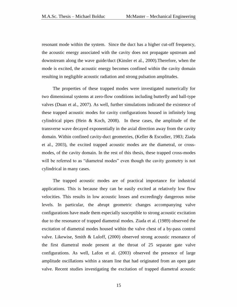
Additional variations of geometry, specifically in the vicinity of the cavity
domain, can affect the trapped nature of the acoustic modes. Experimental tests
conducted by Barannyk & Oshkai (2014) investigated the diametral modes within
an axisymmetric cavity situated in the middle of a converging-diverging section
attached to a larger diameter piping domain. This geometry is commonly found in
control gate valve assemblies within industry. As the angle of the convergence-
divergence section increased, the pulsation amplitudes of the acoustic modes
decreased substantially. Observations of the simulated mode shapes indicated an
increase in acoustic radiation through the attached piping, resulting in a reduction
in the trapped nature of the acoustic modes.
The simulated mode shapes and resonant frequencies, Figure 2-9, were
computed at zero flow velocity conditions. Further numerical simulations, (Aly &
Ziada, 2012), investigated the effect of mean flow on both the resonant
frequencies and mode shapes of the trapped diametral modes. Results indicated
the resonant frequencies decreased slightly with a corresponding increase in Mach
number. As well, the mode shape became more concentrated to the downstream
edge of the cavity, modulated to that of convected flow velocity. Additional
evidence illustrated that the acoustic particle velocity amplitude at the cavity
mouth was largely influenced by this variation in the mode shape. However, both
these variations in acoustic pressure and particle velocity were shown to be
independent of the azimuthal angle.
2.5 Fluid-Resonant Excitation Mechanism
The fluid-resonant excitation mechanism is driven by the interaction
between the flow instability at the upstream cavity edge and the acoustic particle
velocity fluctuations introduced by the resonant sound field. These velocity
fluctuations initiate the growth and amplification of the perturbations all along the
shear layer circumference. Howe’s aerodynamic theory of sound approximates the
acoustic power production, P, from the interaction between the parameters of the

M.A.Sc. Thesis – Michael Bolduc McMaster – Mechanical Engineering
21
flow field, via the vorticity vector, , and mean flow velocity vector, with the
resonant sound field, via the acoustic particle velocity, (Howe, 1980).
P (2.2)
The determination on whether the acoustic resonance is self-sustaining
depends on the sign of the integrated power over one acoustic cycle. If the amount
of energy that is transferred to the resonant sound field is larger than that absorbed
by the vortical structure along one acoustic cycle, then the integrated acoustic
power is positive and resonance is self-sustaining. An illustration of this energy
exchange is represented in Figure 2-13 (Ziada, 2010), corresponding to a
transverse standing wave within a deep cavity.
Figure 2-13: Illustration detailing the energy exchange between the flow field and the resonant sound field during an acoustic cycle of a transverse acoustic mode in a deep cavity (Ziada, 2010)
At the beginning of the acoustic cycle, during the initial vortex rollup, the
acoustic particle velocity is directed towards the cavity walls. Here, the acoustic
energy is being absorbed by the vortical structure, as depicted by its amplification.
It is at this location, where the acoustic particle velocity is most dominant in the
initiation and formation of the vortical disturbances. Further downstream, and
later in the acoustic cycle, the acoustic particle velocity is now acting outwards
towards the centerline of the pipe. At this point in the cycle, the vortical structure

M.A.Sc. Thesis – Michael Bolduc McMaster – Mechanical Engineering
22
is now generating acoustic energy to sustain the resonant sound field. In this
example, the generation of acoustic energy is larger than that absorbed by the
vortical structure, indicating a self-sustained oscillation. As will be discussed later
in this review, this energy exchange may not be synchronized/uniform along the
circumference of the shear layer depending on the excited mode shape and
acoustic particle velocity distribution.
2.5.1 Hydrodynamic Modes or Free Shear Layer Modes
The described energy transfer between the propagating disturbances and
acoustic particle velocity occurs all along the impingement/cavity length. In order
for acoustic resonance to be sustained, a specific phase condition between these
two components must be satisfied. This is to ensure that the vortical structure is
amplified at the upstream edge and that it generates acoustic energy further
downstream.
The fulfilment of this phase constraint can occur at different shear layer
oscillation patterns, corresponding to a varying number of vortices being
propagated along the cavity length. These oscillation patterns are defined free
shear-layer modes, whose modal number, n, designates the number of vortices
present along the cavity length during an acoustic cycle. These shear layer
oscillations occur at well-defined frequencies, described by their dimensionless
Strouhal number shown below, where f represents the respective oscillation
frequency, L represents the cavity length, and U represents the mean flow
velocity.
(2.3)
In the previous case of the h=50.8mm, L/h=0.5 axisymmetric cavity, Figure
2-12, the trapped diametral acoustic modes were excited by the first two free
shear layer modes, n=1 and 2, consisting of one or two vortices propagating along
the cavity length. Figure 2-14 displays the dimensionless acoustic pressure for this

M.A.Sc. Thesis – Michael Bolduc McMaster – Mechanical Engineering
23
cavity geometry and its associated Strouhal number for each of the three diametral
modes during its velocity range of excitation (Aly & Ziada, 2010).
Figure 2-14: Relationship of dimensionless acoustic pressure and Strouhal number during the excitation of the three diametral trapped acoustic modes, h=50.8mm, L/h=0.5 axisymmetric cavity (Aly & Ziada,2010)
As indicated, the Strouhal numbers lie within two distinct ranges,
corresponding to each of the hydrodynamic shear layer modes. The first shear
layer mode occurs for a Strouhal number range 0.2-0.4, and the second occurs at a
Strouhal number from 0.7-0.9. The Strouhal numbers remain fairly constant for
each of the three associated acoustic modes. This is unlike studies involving the
fluid-dynamic feedback where the Strouhal numbers vary inversely in relation to
the Mach number (Tam & Block, 1978).
2.5.2 Distribution of Acoustic Particle Velocity
Based on Howe’s aeroacoustic analogy, the generation, or absorption, of
acoustic power P is most efficient when the three components of the triple
product ( and are perpendicular to each other. In the cases consisting of
an axisymmetric shear layer, the radial component of the acoustic particle velocity
is the energy generating component. However, the distribution and magnitude of
this component will vary depending on the cavity-duct geometry and the acoustic
mode being excited.

M.A.Sc. Thesis – Michael Bolduc McMaster – Mechanical Engineering
24
In the case of longitudinal acoustic modes, the component of the acoustic
particle velocity is parallel to that of the mean flow velocity, . Through the
triple product within Howe’s analogy, the overall acoustic power generated and
absorbed throughout the acoustic cycle would seem to be zero. However, studies
conducted by Hourigan et al. (1990) on a longitudinal mode present in a duct with
baffles, helped illustrate that the acoustic particle velocity included a
perpendicular component to that of the mean flow, arising from the streamline
curvature around the baffle. A similar behaviour is observed at the upstream and
downstream edges of shallow cavities excited by longitudinal acoustic modes
(Mohamed & Ziada, 2014). Since the acoustic properties only vary in the axial
direction, the associated acoustic particle velocity distribution will be uniform
along the shear layer circumference.
For the trapped diametral acoustic modes, however, the acoustic properties
vary along the azimuthal orientation due to its asymmetric mode shape. Contour
plots of the radial acoustic particle velocity distributions for the first three
diametral modes located at the midpoint of the axisymmetric cavity with
h=25.4mm, L/h=1, are shown in Figure 2-15.
Figure 2-15: Radial acoustic particle velocity distribution of the diametral modes within an axisymmetric cavity with h=25.4mm, L/h=1 (Aly & Ziada, 2010)

M.A.Sc. Thesis – Michael Bolduc McMaster – Mechanical Engineering
25
As shown, the radial acoustic particle velocity distribution for each of the
three excited diametral modes is non-uniform and akin to its corresponding mode
shape. Also, the areas with the largest radial particle velocity fluctuations move
outwards in the radial direction as the mode order increases.
These differences in the radial acoustic particle velocity distributions lead to
two unique excitation mechanisms. For longitudinal acoustic modes, since the
radial particle velocity is uniform along the whole circumference of the
axisymmetric shear layer, the energy exchange and excitation of disturbances all
along the circumference and length of the cavity shear layer is synchronized.
However, in the case of the diametral modes in Figure 2-15, the excitation
mechanism, and energy exchange, is three-dimensional and much more complex.
The radial acoustic particle velocity fluctuations are non-uniform along the shear
layer circumference and different circumferential sections of the shear layer may
be excited out of phase and at various amplitudes. The distribution of these
particle velocity fluctuations is dictated by the relative position to the acoustic
mode shape and its associated nodal lines.
2.6 Effects of Symmetry on the Diametral Modes
The excitation of an asymmetric diametral mode housed within an
axisymmetric cavity configuration leads to non-preferred orientations of the
simulated mode shapes displayed in Figure 2-9. The symmetry incorporated with
the cylindrical geometry ensures that there are an infinite amount of mode shapes
corresponding to each eigenvalue (resonant frequency) that is resolved from the
Helmholtz equation (Morse, 1948).
In the case of the first acoustic mode, each of these mode shapes
corresponds to a unique angular orientation of its nodal line. In most cases of
degeneracy, the preferred mode shape would depend on the orientation where the
system is initially excited, fixing the mode in a particular orientation (Kinsler et
al., 2000; Morse, 1948). However, the axisymmetric shear layer is excited wholly

M.A.Sc. Thesis – Michael Bolduc McMaster – Mechanical Engineering
26
along the circumference of the upstream edge. This results in the acoustic mode to
spin about its axis at a rate equal to its resonant frequency. This behaviour is
referred to in literature as a fully spinning mode (Aly & Ziada, 2011).
In addition to the work done on axisymmetric cavities, previous
investigations on spinning, or turning, azimuthal modes have been detected in
axisymmetric geometries in applications involving stator/rotor interactions (Tyler
& Sofrin, 1962) and transverse thermo-acoustic instabilities within annular
combustion chambers as detailed in the review by O’Connor et al. (2015).
Experiments on trapped diametral acoustic modes within axisymmetric
cavities observed fully spinning behaviour when the cavity was perfectly
axisymmetric (Aly & Ziada, 2011). If a large amount of asymmetry was
introduced into the cavity domain, then a preferred orientation would be
introduced and the acoustic mode would remain stationary. This was observed in
experiments conducted by Keller & Escudier (1983) where the orientation of
stationary diametral modes within a confined axisymmetric cavity varied when
the assembly was taken apart and reassembled. Likewise, if only a slight amount
of asymmetry is introduced within the geometry, an intermediate “partially
spinning” behaviour is observed (Aly & Ziada, 2011). Within annular combustors,
asymmetry can be introduced through flame merging (through reduction in
spacing) and introducing baffles, resulting in the partially spinning and fully
stationary transverse modes (Worth & Dawson, 2013 & 2015).
A spinning mode can be visually represented along its acoustic cycle
through the combination of two equivalent orthogonal stationary modes, Figure 2-
16, with a 90˚ temporal phase shift. Depending on the relative amplitudes of these
two orthogonal modes, different azimuthal behaviours are obtained. If this
amplitude ratio is zero, A/B=0, the resultant mode is identical to the stationary
orthogonal mode with non-zero amplitude, B. If the two amplitudes are equal, the
resultant mode will be a fully spinning mode. If the amplitudes are not equal and

M.A.Sc. Thesis – Michael Bolduc McMaster – Mechanical Engineering
27
larger than zero, then the previously mentioned intermediate partially spinning
mode is obtained.
Figure 2-16: Schematic of two equivalent orthogonal modes with amplitudes A & B
This two orthogonal model has been utilized in different studies involving
the representation of spinning modes within axisymmetric cavities (Aly, 2008), as
well as in combustion chambers (Worth & Dawson, 2013; Salle et al., 2004 &
2006) for example. A graphical comparison of the spinning mode (left) and
partially spinning mode (right) for an axisymmetric cavity at six equal interval
phases through a half-cycle are displayed in Figure 2-17 (Aly, 2008).
Figure 2-17: Comparison of the fully spinning, A/B=1, (left) and partially spinning, A/B=0.4, (right) acoustic modes within an axisymmetric cavity along six equal interval phases of its half acoustic cycle
(Aly, 2008)
M.A.Sc. Thesis – Michael Bolduc McMaster – Mechanical Engineering
28
For both spinning modal behaviours, the nodal line of the mode rotates at
the excited resonant frequency. In the case of the fully spinning mode (left) the
acoustic pressure distribution remains constant about its rotating nodal line.
However, for the partially spinning mode (right), this distribution varies in a
sinusoidal manner along the azimuthal direction, similar to that of a stationary
diametral mode. This variation in acoustic pressure along one full cycle is
determined by the relative ratio of A/B.
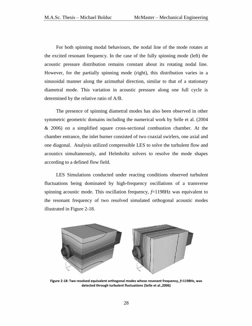
The presence of spinning diametral modes has also been observed in other
symmetric geometric domains including the numerical work by Selle et al. (2004
& 2006) on a simplified square cross-sectional combustion chamber. At the
chamber entrance, the inlet burner consisted of two coaxial swirlers, one axial and
one diagonal. Analysis utilized compressible LES to solve the turbulent flow and
acoustics simultaneously, and Helmholtz solvers to resolve the mode shapes
according to a defined flow field.
LES Simulations conducted under reacting conditions observed turbulent
fluctuations being dominated by high-frequency oscillations of a transverse
spinning acoustic mode. This oscillation frequency, f=1198Hz was equivalent to
the resonant frequency of two resolved simulated orthogonal acoustic modes
illustrated in Figure 2-18.
Figure 2-18: Two resolved equivalent orthogonal modes whose resonant frequency, f=1198Hz, was detected through turbulent fluctuations (Selle et al.,2006)

M.A.Sc. Thesis – Michael Bolduc McMaster – Mechanical Engineering
29
From the symmetry inherent within the square geometry, there were two
orthogonal mode shapes corresponding to the same resonant frequency. This
provides no preferential orientation to the excitation of either of the two acoustic
modes, and similar to the axisymmetric domain, results in a spinning behaviour.
Utilizing the two mode orthogonal mode, the acoustic mode shape and the
axial acoustic particle velocity along one acoustic cycle were resolved and
visually represented. The influence of the acoustic mode was then compared to
the simulated flame structure from LES. These results are taken at a field-of view
shown in Figure 2-19, and are represented along half an acoustic cycle in Figure
2-20.
Figure 2-19: Cross-sectional view used in the visualization of the acoustic spinning mode (Selle et al.,2006)
As shown, the acoustic mode rotates about the cavity at its resonant
frequency. The acoustic particle velocity contour is non-uniform along the burner
mouth and is 90˚ out of phase with the acoustic pressure distribution. This is quite
different to the uniform excitation of the shear layer associated with the
longitudinal mode. Instead, only specific sections of the shear layer are being
excited at a time and these sections are now rotating about the circumference of
the burner. As such, the resolved flame structure is of a helical type and is akin to
the particle velocity fluctuations acting along the upstream edge.

M.A.Sc. Thesis – Michael Bolduc McMaster – Mechanical Engineering
30
Figure 2-20: Simulated mode shape (left), axial acoustic particle velocity (middle), and helical structure (right) during half an acoustic cycle of the spinning acoustic mode (Selle et al.,2006)
M.A.Sc. Thesis – Michael Bolduc McMaster – Mechanical Engineering
31
2.7 Noise Control of Trapped Diametral Modes
The suppression of acoustic resonance from grazing flows over cavities has
been investigated extensively within literature. These mitigation techniques are
implemented when acoustic resonance is undesirable and avoidance is not
possible. Control methods are generally categorized as being either active or
passive.
Active control involves applying external energy into the system and
involves methods such as oscillating flaps and pulsed fluid injection (Cattafesta et
al., 2003). The cost of installation and its separate components make active
control generally impractical within industrial applications, particularly in the
case of a confined cavity domain. Nonetheless, it has been successfully
implemented in reducing the acoustic resonance of trapped diametral modes in
laboratory settings. Ziada et al. (2003) utilized a synthetic jet generated from two
loudspeakers positioned at the upstream cavity corner. The externally applied
acoustic pressure successfully cancelled out the interaction with the acoustic
particle velocity, suppressing the acoustic resonance.
Many studies have focused on passive remedial means, involving geometric
modifications situated at the upstream edge of the cavity. The focus of these
modifications is to influence the initiation and formation of vortical structures
from the interaction with the resonant sound field. Experiments conducted by
Smith & Luloff (2000) investigated the effects of chamfering the upstream edge
in reducing acoustic resonance within gate valves. This provided an overall
reduction in acoustic pressure; however the acoustic mode shapes within the valve
were not indentified and the influence of the chamfers on the global aeroacoustic
response was unreliable.
Recently, Bolduc et al. (2014) investigated passive modifications at the
upstream edge of the axisymmetric cavities used in the previous studies by Aly &
Ziada (2010, 2011, 2012). Schematics of these modifications are illustrated in

M.A.Sc. Thesis – Michael Bolduc McMaster – Mechanical Engineering
32
Figure 2-21. The dimensions utilized for these experiments were based on
previous studies involving the mitigation of longitudinal acoustic modes
(Bruggeman et al., 1991; Karadogan & Rockwell, 1983; Knotts & Selamet, 2003;
akibo lu & Hirschberg, 2010).
The first geometric modifications consisted of chamfering and rounding the
upstream cavity edge, which both delayed the acoustic resonance to higher
velocity ranges. This was a direct result of altering the effective impingement
length the vortices travel along the cavity. With the length changing, and the
resonance Strouhal number remaining constant, the velocity at which acoustic
resonance occurs increases. However, the rounding managed to increase the
pulsation amplitudes, consistent with mitigation studies of closed side-branches
(Bruggeman et al., 1991).
Figure 2-21: Schematic of geometric modifications at the upstream cavity edge. From left to right, sharp edge, rounding, chamfering, and saw-tooth spoiler (Bolduc et al., 2014)
Figure 2-22: Photograph illustrating upstream geometric modifications of the curved and delta spoilers at the shear layer (Bolduc et al., 2014)

M.A.Sc. Thesis – Michael Bolduc McMaster – Mechanical Engineering
33
In addition, assortments of spoiler geometries were examined. These
included various saw-tooth spoilers, a curved spoiler and a unique delta spoiler
shown in Figure 2-21 and 2-22. These spoilers were situated all along the
circumference of the shear layer, due to the spinning nature of the acoustic mode,
and were designed to introduce additional three-dimensional vorticity and
turbulence to reduce the coherence of the vortical structures. This in turn, would
reduce the flow-sound coupling of the propagating disturbances with the resonant
sound field.
The introduction of these spoilers reduced the pulsation amplitude of the
acoustic modes significantly, but had an undesirable economic outcome.
Depending on the spoiler size, the flow blockage introduced a significant amount
of pressure drop within the system. This effect would need to be minimized in
order to maintain maximum efficiency within the operations of BWR and PWR
plants.
2.8 Objectives
The previous studies investigating the excitation of trapped diametral
acoustic modes within cavity-duct domains have focused on axisymmetric
geometries. These geometries lead to spinning modal behaviours due to there
being no preferred orientation. There has been little attention on asymmetric
rectangular cross-sectional cavity-duct domains, which results in the trapped
diametral modes being fixed in one unique orientation. This effect of symmetry is
investigated in regards to its modal behaviour, trapped nature, and aeroacoustic
response.
As well, inspection of rectangular cavity geometries provides some practical
benefits over the previous axisymmetric cases. Through removal of the complex
spinning nature of the acoustic modes, this provides a simpler model for
validation of numerical simulations. Currently, the experimental results obtained
from this study are being used to improve CFD codes in the prediction of onset
M.A.Sc. Thesis – Michael Bolduc McMaster – Mechanical Engineering
34
excitation velocities, pulsation amplitudes, and the acoustic modes for simplified
gate valve geometries. Through improvement of numerical simulations, this may
provide a means to a better understanding of the excitation mechanism and a
design tool for future applications.
The excited acoustic modes are the transverse diametral (cross) modes
confined within the cavity. The acoustic properties of these diametral modes vary
in the azimuthal direction. Thus, the radial acoustic particle velocity and
excitation of the shear layer is non-uniform along the circumference. As well,
these associated modes are trapped and consist of very strong acoustic resonance.
Despite this complex excitation mechanism, orderly flow structure must occur in
order to generate sufficient acoustic energy to maintain these strong pulsation
amplitudes. Thus far, little work has been done on understanding this three-
dimensional flow-sound coupling between the non-uniform acoustic particle
velocity and its propagating structures.
Understanding this excitation mechanism of these complex acoustic modes
will expand upon the state of knowledge in the potential of noise suppression
techniques that not only mitigate acoustic resonance but do so with minimal
pressure drop.
In summary, there are two main objectives within this study:
Investigate the effects of velocity and asymmetry on the excitation
mechanisms and trapped nature of the acoustic modes within rectangular
cavities.
Investigate the three-dimensional flow-acoustic coupling between the non-
uniform acoustic particle velocity of the excited diametral modes and the
corresponding downstream propagating structures.

M.A.Sc. Thesis – Michael Bolduc McMaster – Mechanical Engineering
35
CHAPTER 3 EXPERIMENTAL APPARATUS
This chapter focuses on the experimental facility and test setup that was
designed and utilized to investigate the flow-excited acoustic resonance of trapped
diametral modes within a rectangular cavity-duct domain. Section 3.1 details the
test facility and piping, which is consistent with previous studies involving the
excitation of diametral modes in axisymmetric cavities (Aly & Ziada, 2010, 2011,
2012; Bolduc et al.,2013). However, the asymmetric rectangular cavities, Section
3.2, were designed and manufactured to introduce a preferred orientation for the
excited diametral modes. Section 3.3 examines the asymmetric acoustic mode
shapes and the trapped nature of the acoustic modes, leading to the resolved
acoustic particle velocity distributions in Section 3.4. Finally, Section 3.5 details
the instrumentations used throughout the measurements.
3.1 Test Facility
A schematic of the test-facility and its components is shown in Figure 3-1.
The open loop wind tunnel consists of a 10 blade centrifugal blower powered by a
50hp electric motor. The inlet flow velocity is altered by the rotational speed of
the blower through a variable speed control unit. The velocity was altered in a
separate room to avoid extended exposure to the high sound pressure levels.
Measurements were conducted up to the maximum capacity of the blower at
a Reynolds number of ReD= based off the duct diameter and the velocity
measured at the bell-mouth end. The cavity test setup is installed to the inlet,
transitioning to an axisymmetric diffuser, until reaching the centrifugal blower.
The design of the diffuser was selected from CFD simulations to determine
applicable dimensions (Aly, 2008). To ensure the test setup does not move when
the flow velocity is changed, chains and a flexible hose to isolate the blower
velocity were installed.

M.A.Sc. Thesis – Michael Bolduc McMaster – Mechanical Engineering
36
1 Test Setup
2 Chains
3 Axisymmetric
Diffuser
4 Centrifugal Blower
5 Control Unit
6 Electric Motor
7 Settling Chamber
8 Wind Tunnel Outlet
Figure 3-1: Schematic of Test Facility and its components.

M.A.Sc. Thesis – Michael Bolduc McMaster – Mechanical Engineering
37
3.2 Test Setup
The test section was designed specifically to analyze the excitation of
diametral modes within a rectangular cavity. An illustration of the cavity-duct
setup is shown in Figure 3-2. The system consists of three main components: the
upstream/downstream piping, the cavity domain, and the bell mouth inlet. The
inlet and the piping system remained consistent to the investigations of
axisymmetric cavities conducted by Aly & Ziada (2010, 2011, 2012). However,
three new rectangular cross-sectional cavities were designed, manufactured, and
installed.
Figure 3-2: Schematic of Test Setup (Aly & Ziada, 2010)
Upstream and downstream of the cavity consisted of two =450mm long
clear acrylic pipes. The inner diameter of these pipes, D, was 150mm and had a
thickness of 6.25mm. Numerical simulations, discussed in Section 3.3, illustrate
that the ample lengths of the pipes do not alter the acoustic mode shapes. At the
terminations of the pipes are two flanges to connect the cavity domain to the
piping system. O-rings and gaskets were used in between the flanges and the
pipes to ensure proper sealing and to minimize acoustic losses from the system.
Two sets of eight pressure taps were installed at 45˚ intervals along the
circumference of the piping system. The taps were located 30cm upstream and
downstream from the cavity edges to measure the static pressure drop across the
cavity domain. This large number of pressure taps along the circumference was

M.A.Sc. Thesis – Michael Bolduc McMaster – Mechanical Engineering
38
chosen to ensure that the average static pressure was a good representation of the
pressure drop whether the excited diametral mode was spinning or stationary.
The inlet of the system consisted of a smooth bell mouth. It had a parabolic
contraction to ensure that the mean velocity profile was uniform within the pipe
and that the turbulence intensity was minimized. A non-uniform velocity profile,
particularly along the upstream shear layer, may result in unwanted disturbances
influencing the excitation of the diametral modes. Thus, much care was placed to
ensure the contraction was as smooth and uniform as possible
3.2.1 Cavity Geometry
Three separate cavities were manufactured and tested. A generalized
schematic of the cavity geometry is shown in Figure 3-3. All manufactured
cavities had a length of L=25.4mm and constant height of H =254mm. The
difference in geometry is due to variations in the width, W, where only slight
variations from unity (W/H=0.9-0.95) were considered for the two rectangular
cavities. The dimensions of the manufactured cavities are listed in Table 3-1.
Figure 3-3: Schematic of cavity dimensions and geometry
Table 3-1: Dimensions of three manufactured cavities, L=25.4mm and H=254mm
Type W/H H (mm) W (mm)
Square 1 254 254
Rectangular 1 0.95 254 241.3
Rectangular 2 0.9 254 228.6

M.A.Sc. Thesis – Michael Bolduc McMaster – Mechanical Engineering
39
The reference dimensions for the square cavity were selected by reviewing
the aeroacoustic responses of axisymmetric cavities (Aly & Ziada, 2010). The
chosen L=25.4mm and W=H=254mm square geometry is close to the
axisymmetric cavity with L/h=0.5, h/D=1/3, which produced strong resonance of
the first three modes. The dimensional comparisons and aeroacoustic response are
shown in Figures 3-4 and 3-5.
This axisymmetric cavity held preferential characteristics in its aeroacoustic
response when compared to its counterparts. As observed in Figure 3-5, there was
evidence of numerous diametral trapped modes being excited at lower velocity
ranges providing a means to compare and observe the excitation mechanisms of
multiple diametral modes within the capacity of the blower. The excitation at
lower flow velocities also reduces the likelihood of complications arising from the
use of Particle Image Velocimetry including the buildup of seeding particles and
the required time delay between consecutive images.
Figure 3-4: Dimensional comparisons between axisymmetric and present square cavity (dashed).
Figure 3-5: Dimensionless aeroacoustic pressure response for axisymmetric cavity, L/h=0.5, h/D=1/3
(Aly & Ziada, 2010)

M.A.Sc. Thesis – Michael Bolduc McMaster – Mechanical Engineering
40
The geometries of the two rectangular cavities were selected to introduce
asymmetry to the reference square cross-section. Only slight deviations from the
square cavity were considered, (W/H=0.9 & 0.95), introducing two orthogonal
resonance modes that have comparable, yet slightly offset frequencies (0% for the
square and 9% for rectangular cavity 2). Comparisons of the three cavity
geometries would provide insight on the effects of asymmetry on both the
aeroacoustic responses and the behaviours of the excited diametral modes.
3.2.2 Test Section Assembly
The cavities are constructed from two sets of acrylic side walls which are
assembled together using clamps, threaded rods, gaskets and silicon to ensure
proper sealing and to produce the assembly which is illustrated in Figure 3-6. For
the three manufactured cavities, three similar pairs of side walls were used for the
constant 254mm height. To alter the varying cavity width, W, another three pairs
for the top and bottom were installed depending on the desired cavity geometry.
The dimensions of these sets of side-walls are detailed in Figures 3-7 and-3-8 and
Table 3-2. As well, additional holes were machined into the cavity walls to allow
dynamic pressure transducers to remain flush to the inner cavity wall coinciding
with the anti-nodes of each of the investigated diametral modes.
Figure 3-6: Detailed exploded assembly of test section
1 Piping
2 Flange
3 Constant side wall
4 Variable top wall

M.A.Sc. Thesis – Michael Bolduc McMaster – Mechanical Engineering
41
Figure 3-7: Dimensions (mm) of Constant side wall used in all three cavities
Figure 3-8: Dimensions (mm) of Variable top and bottom walls with varying dimension X
Table 3-2: Dimensions (mm) of variable x corresponding to the three separate manufactured cavities
To attach the side lengths to the upstream and downstream piping, and to
clamp the cavity in place, two acrylic square flanges were manufactured on a
CNC milling machine. Eight holes with transition fits were machined into the
flanges coinciding with holes positioned in the side lengths and clamped using
threaded rods. The CNC was also utilized to remove any potential non-uniformity
at the upstream and downstream corners of the cavity in accordance to the piping.
This procedure allowed proper and consistent alignment of the cavity with the
pipe diameter. O-rings, gaskets and silicon sealing were applied on the interfaces
between the cavity, flanges, and piping to remove any potential sources of
leakage. This overall assembly of the test setup provided easy transition between
cavity geometries, proper sealing, and optical clarity for flow visualization.
Type W/H W (mm) X (mm) Square 1 254 25.4
Rectangular 1 0.95 241.3 19.05
Rectangular 2 0.9 228.6 12.7

M.A.Sc. Thesis – Michael Bolduc McMaster – Mechanical Engineering
42
3.3 Numerical Simulations
3.3.1 Simulation and Mesh Configuration
The distribution of acoustic pressure, P, for the three-dimensional trapped
diametral acoustic modes can be resolved through the three-dimensional wave
equation:
(3.1)
where c is the speed of sound, and represents the Laplacian represented
below in Cartesian coordinates:
(3.2)
The oscillating pressure field of the acoustic modes is a harmonic function
in time, t, and can written as:
(3.3)
where is the spatial distribution of the acoustic pressure and is the
angular resonance frequency of the mode. Substituting equation (3.3) into
equation (3.1) the Helmholtz equation is obtained:
(3.4)
Commercial FEA software ABAQUS was utilized to numerically solve this
eigenvalue problem at zero flow conditions. The resultant eigenfunctions
represent the dimensionless acoustic pressure distribution (the mode shapes), and
the eigenvalues are the corresponding resonant frequencies. The computational
mesh is composed of three-dimensional linear tetrahedral elements consisting of
four nodes. The domain is composed of air with properties at room conditions
with a density
and an adiabatic bulk modulus, K=142000Pa.

M.A.Sc. Thesis – Michael Bolduc McMaster – Mechanical Engineering
43
Realistic boundary conditions were utilized to fully represent the physical
problem. For a fully trapped mode, the end effects would have no influence on the
acoustic pressure distribution within the cavity domain. As such, the acoustic
pressure was set to zero at the terminations of the pipe to represent free ends with
negligible radiation. As well, solid wall conditions at the surfaces were defined to
ensure that pressure gradient was zero at these boundaries.
Additional simulations verified the pipes were of ample length, with any
additional length having no influence on the trapped mode shapes and resonant
frequencies. Figure 3-9 demonstrates the variation in resonant frequency with
changes in pipe length per diameter, /D, for the first resolved mode in the
W/H=0.9 rectangular cavity. After two pipe diameters, both upstream and
downstream, the pipe length has a negligible effect, around 0.001%, on the
resonant frequency. Therefore, a final length of three pipe diameters was used in
the computation, consistent to the experimental setup.
Figure 3-9: Influence of pipe length per diameter ( /D) on simulated resonant frequency, W/H=0.9, first acoustic mode
The convergence of the W/H=0.9 cavity’s first resonant frequency, with an
increase in elements, is shown in Figure 3-10. As the number of elements
increased from to , the resonant frequency varied slightly by

M.A.Sc. Thesis – Michael Bolduc McMaster – Mechanical Engineering
44
0.035%. Thus a conservative number of elements, , consisting of a
global element size of 0.00275mm were used within the simulation. This large
number of elements ensured that there was a sufficient amount of nodal points
along the circumference of the upstream shear layer for the eventual resolved
acoustic particle velocity distribution. At the junctions of the upstream and
downstream ducts with the cavity domain, sharp edges were also rounded with a
radius of 0.6mm to remove any singularities.
Figure 3-10: Convergence of first resonant frequency with increasing number of elements, W/H=0.9 rectangular cavity
3.3.2 Simulated Trapped Diametral Acoustic Modes
The resolved acoustic mode shapes for the W/H=0.9 rectangular cavity are
presented in Figure 3-11. The cross-sectional views are situated within the middle
of the cavity where the dashed lines represent the nodal lines. These four acoustic
trapped modes are classified from f1-f4 in sequence of increasing resonant
frequency and onset excitation flow velocity. As shown, the acoustic modes are
non-uniform along the cavity perimeter.
The first two trapped modes are orthogonal to one another and consist of a
single nodal line and a half wavelength along their respective side length. The
first mode is associated with the longer side, H, and consists of a larger half
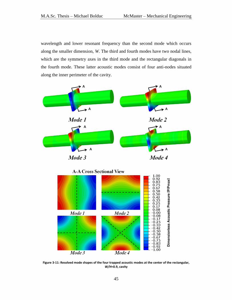
M.A.Sc. Thesis – Michael Bolduc McMaster – Mechanical Engineering
45
wavelength and lower resonant frequency than the second mode which occurs
along the smaller dimension, W. The third and fourth modes have two nodal lines,
which are the symmetry axes in the third mode and the rectangular diagonals in
the fourth mode. These latter acoustic modes consist of four anti-nodes situated
along the inner perimeter of the cavity.
Figure 3-11: Resolved mode shapes of the four trapped acoustic modes at the center of the rectangular, W/H=0.9, cavity

M.A.Sc. Thesis – Michael Bolduc McMaster – Mechanical Engineering
46
The four acoustic modes are trapped with the acoustic energy being highly
localized within the cavity domain and the pressure amplitude exponentially
decaying in the axial direction. This is consistent to simulations previously
conducted for the trapped modes within axisymmetric cavities (Aly & Ziada,
2010). Locally, the confinement of acoustic energy becomes greater in the
outwards radial direction from the attached piping. This observed behaviour is
most prominent within the first two acoustic modes where the mode shape tends
to get modulated by the curvature of the piping. Instead of the anti-node pressure
being present all along the cavity’s height or width, the maximum pressure
pulsations are situated within the corners of the cavity and decrease towards the
midpoints of the side lengths.
As one of the cavity sides gets smaller, the radial distance between the
cavity perimeter and the piping gets shortened. This results in increased acoustic
radiation into the upstream and downstream pipes, which weakens the trapped
nature of the mode. This behaviour may be observed through comparisons of the
first and second mode shapes in Figure 3-11. For the first mode, larger pressure
pulsations are located within the middle of its side lengths, due to the height, H,
having a larger radial distance from the piping curvature than the width, W,
which is associated with the second acoustic mode. As W/H approaches unity,
these two orthogonal simulated mode shapes become equivalent. A similar
behaviour is also observed when comparing the mode shapes of the fourth
acoustic mode for the three cavity geometries
These four trapped diametral modes are strongly excited in each of the three
tested cavities. An additional fifth trapped mode was also detected within
experiments and simulations, consisting of six anti-nodes along the cavity
perimeter. However, because of its additional complexity and that its full
resonance range was beyond the maximum capacity of the blower, this mode is
not addressed here. It is important to note that the main objective of this study is
to investigate the interaction between the resonant sound field and flow field for

M.A.Sc. Thesis – Michael Bolduc McMaster – Mechanical Engineering
47
simplified geometric mode shapes. The simulated resonance frequencies of the
four acoustic modes are given in Table 3-3 for the three investigated cavities.
Table 3-3: Simulated resonant frequencies of the four trapped acoustic modes for the three cavity geometries
The trapped nature of the acoustic mode depends on the ratio of the resonant
frequency to the cut-off frequency of the attached piping. As this ratio decreases,
more acoustic energy is confined within the cavity and less is radiated axially
down the piping (Kinsler et al., 2010). The first two calculated cut-off frequencies
of the pipes, 1307Hz and 2166Hz, correspond to one and two nodal lines. The
first resonant frequencies, f1 and f2 (855-954Hz), consist of one nodal line and are
much lower than those associated with the first cut-off frequency. Likewise f3 and
f4 (1027-1610Hz) consist of two nodal lines and are significantly lower than the
second cut-off. Since these acoustic modes of the cavity are inherently three-
dimensional, changing the dimension of one side of the cavity (e.g., width W) has
a slight effect on the resonance frequency of the mode along the other dimension,
H, as illustrated through the small variations in the first resonant frequency.
For the square cavity, since H is equal to W, the associated wavelengths and
resonant frequencies of the first two orthogonal modes are identical. This is
commonly referred to in literature as a degenerate mode (Kinsler et al., 2010)
(Morse, 1948). From the symmetry inherent within the square cross-sectional
geometry, the solution of the Helmholtz equation resolves two separate
eigenfunctions coinciding to one distinct eigenvalue, providing no preferential
orientation to the excitation of either of the two orthogonal modes. The excitation
of this degenerate mode results in a unique spinning behaviour that will be
discussed in detail within the experimental results.
Resonant Frequencies (Hz)
W/H f1 f2 f3 f4
1 855 855 1027 1500 0.95 866 903 1059 1550
0.9 878 954 1097 1610

M.A.Sc. Thesis – Michael Bolduc McMaster – Mechanical Engineering
48
3.4 Acoustic Particle Velocity
The excitation mechanism is due to a flow-acoustic coupling between the
resonant sound field, via the acoustic particle velocity, , the flow field, via the
vorticity vector, , and the mean flow velocity vector, . Howe’s aerodynamic
theory of sound approximates the acoustic power production, P, from the
interaction between each of these variables (Howe, 1980).
P (3.5)
As demonstrated in the above expression, the generation, or absorption, of
acoustic power P is largest when all three components of the triple product (
and are orthogonal to one another. In the current case involving an
axisymmetric shear layer, illustrated in the schematic Figure 3-12, it is the radial
component of the acoustic particle velocity which is orthogonal to both the shear
layer vorticity, and mean flow velocity, . The radial velocity fluctuations,
due to the resonance of the acoustic mode, initiate the formation of disturbances
along the circumference of the upstream separation edge.
Figure 3-12: Simplified schematic of a uniform radial acoustic particle velocity vector distribution, ,
represented by dashed vectors. This initiates the formation of disturbances at the upstream axisymmetric separation edge.

M.A.Sc. Thesis – Michael Bolduc McMaster – Mechanical Engineering
49
The simplified schematic in Figure 3-12 displays a uniform distribution of
radial acoustic particle velocity along the shear layer circumference at the cavity
upstream edge. This distribution, consistent to that of a longitudinal acoustic
mode, would result in a synchronized triggering of the whole shear layer
circumference. The resultant formation of disturbances would be uniform and
would consist of a toroidal vortex, or vortex ring, propagating downstream.
However, in the present study, the simulated diametral trapped acoustic
modes are non-uniform and asymmetric about the cavity. As such, the associated
radial acoustic particle velocity along the shear layer circumference will vary.
Assuming an adiabatic process, the distributions of acoustic particle velocity of
each of the simulated diametral modes can be resolved from the three-dimensional
pressure gradient, via Euler’s equation:
(3.6)
Assuming simple harmonic motion, the acoustic particle velocity, may
be rearranged as follows:
(3.7)
For each of the simulated acoustic modes, the three-dimensional pressure
gradients, , were determined through the acoustic pressure distributions in
their FEA simulations. A code developed specifically for three-dimensional linear
tetrahedral 4-node elements was utilized and validated against closed-form
solutions. From the above method, a three dimensional distribution of the acoustic
particle velocity is resolved.
Emphasis is placed at the upstream edge of the shear layer, where the
formation of vortical structures is initiated by the radial acoustic particle velocity.
Thus, the radial component can be extracted from the three dimensional velocity

M.A.Sc. Thesis – Michael Bolduc McMaster – Mechanical Engineering
50
vectors along the separation edge. However, to avoid potential singularities at the
edges of the cavity and piping, all presented distributions are located slightly
offset, 0.2mm, from the upstream separation edge.
3.4.1 Radial Acoustic Particle Velocity Distributions
Figure 3-13 presents normalized contour plots from the initial simulated
acoustic mode shape to the extracted radial acoustic particle velocity vectors
along the shear layer circumference near the cavity upstream corner. These figures
are associated with the second acoustic mode of the W/H=0.9 rectangular cavity
with the cavity corner being represented by the circular line. As clearly displayed,
unlike the longitudinal mode, the radial acoustic particle velocity distribution is
non-uniform along the shear layer circumference and its distribution is akin to its
asymmetric mode shape.
Figure 3-13: Dimensionless (Top Left) Acoustic pressure distribution, (Top Right) Acoustic particle velocity
magnitude, (Bottom Left) Radial acoustic particle velocity distribution, (Bottom Right) Radial particle velocity along shear layer circumference (all figures correspond to 0.2mm downstream from the inlet of
the W/H=0.9 rectangular cavity)

M.A.Sc. Thesis – Michael Bolduc McMaster – Mechanical Engineering
51
Likewise, the radial acoustic particle velocity distributions of the remaining
three acoustic modes and their acoustic pressure distributions are shown in Figure
3-14. Similar to the second acoustic mode, the radial acoustic particle velocity
closely resembles the acoustic mode shape. The points of zero radial velocity
fluctuations correspond to the nodal pressure lines, and the maximum radial
velocity amplitudes coincide to the anti-nodes of the associated mode. As well, the
radial acoustic particle velocity oscillations occur along specific circumferential
portions of the shear layer separated by their nodal points. The first two acoustic
modes consist of two circumferential sections, and the third and fourth
corresponding to four. Further investigation of the non-uniform acoustic velocity
distribution and their effect on the development of vortical disturbances will be
focused upon within the experimental results.
Figure 3-14: Normalized acoustic pressure distribution and corresponding radial acoustic particle velocity
along the upstream cavity mouth for the W/H=0.9 rectangular cavity

M.A.Sc. Thesis – Michael Bolduc McMaster – Mechanical Engineering
52
3.4.2 Effect of Geometry
The dimensionless radial acoustic particle velocity distributions for the
W/H=0.9 rectangular cavity are displayed in Figure 3-15 as a function of angle
along the shear layer circumference at the upstream cavity corner and in the
counter-clockwise direction.
Figure 3-15: Dimensionless Acoustic Particle velocity distributions of the four acoustic modes for the
rectangular, W/H=0.9, cavity. All cases correspond to the upstream cavity corner
Due to the asymmetry present within the W/H=0.9 rectangular cavity,
disparity between the radial acoustic particle velocity distributions is observed
between the two orthogonal modes. For the first acoustic mode corresponding to
the larger height, H, the radial particle velocity remains fairly constant along its
two circumferential sections in the ranges of 135-225˚and 315-45 ˚with a slight
drop in amplitude at the midpoints of the side lengths at 0˚ and 180˚. However, in
the case of the second acoustic mode, which is situated along the smaller width,
W, the drop in acoustic particle velocity occurring at 90˚ and 270˚ is much more
significant with an overall reduction of 15%.
The discrepancy between the two distributions are a result of the second
acoustic mode being less trapped and closer to the piping circumference, leading

M.A.Sc. Thesis – Michael Bolduc McMaster – Mechanical Engineering
53
to a reduction in the pressure gradient and resultant radial acoustic particle
velocity. Similar behaviour is observed through comparing the distributions of
second acoustic mode for each of the three simulated cavity geometries, shown in
Figure 3-16.
Figure 3-16: Comparison of dimensionless radial particle velocity distribution for the second acoustic mode as a function of angle, , along the upstream cavity corner of the three cavity geometries
Once again, the reduction in acoustic particle velocity around 90˚ and 270˚
becomes larger as the cavity becomes smaller and more asymmetric. Nonetheless,
this behaviour is not observed for all four trapped modes with changes in cross-
sectional geometry. Comparisons of the particle velocity distributions of the third
acoustic mode are shown in Figure 3-17.
Figure 3-17: Comparison of dimensionless radial particle velocity distribution for the third acoustic mode as a function of angle, , along the upstream cavity corner of the three cavity geometries
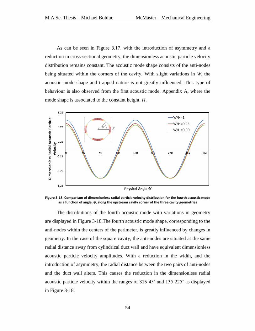
M.A.Sc. Thesis – Michael Bolduc McMaster – Mechanical Engineering
54
As can be seen in Figure 3.17, with the introduction of asymmetry and a
reduction in cross-sectional geometry, the dimensionless acoustic particle velocity
distribution remains constant. The acoustic mode shape consists of the anti-nodes
being situated within the corners of the cavity. With slight variations in W, the
acoustic mode shape and trapped nature is not greatly influenced. This type of
behaviour is also observed from the first acoustic mode, Appendix A, where the
mode shape is associated to the constant height, H.
Figure 3-18: Comparison of dimensionless radial particle velocity distribution for the fourth acoustic mode
as a function of angle, , along the upstream cavity corner of the three cavity geometries
The distributions of the fourth acoustic mode with variations in geometry
are displayed in Figure 3-18.The fourth acoustic mode shape, corresponding to the
anti-nodes within the centers of the perimeter, is greatly influenced by changes in
geometry. In the case of the square cavity, the anti-nodes are situated at the same
radial distance away from cylindrical duct wall and have equivalent dimensionless
acoustic particle velocity amplitudes. With a reduction in the width, and the
introduction of asymmetry, the radial distance between the two pairs of anti-nodes
and the duct wall alters. This causes the reduction in the dimensionless radial
acoustic particle velocity within the ranges of 315-45˚ and 135-225˚ as displayed
in Figure 3-18.

M.A.Sc. Thesis – Michael Bolduc McMaster – Mechanical Engineering
55
3.5 Instrumentation
3.5.1 Dynamic Pressure Transducers
Four PCB piezoelectric dynamic pressure transducers were installed flush
along the cavity interior. The locations of these transducers are placed within the
anti-nodes of the four trapped acoustic modes, as shown in Figure 3-19. The first
two pressure transducers, PT1 & PT2, were installed at the middle of the width,
W, and height, H, coinciding to the anti-nodes of the fourth acoustic mode. The
remaining two dynamic pressure transducers, PT3 & PT4, are located within two
corners of the cavity coinciding to the anti-nodes of the first three acoustic modes.
These four transducers are used simultaneously during measurements to ensure
that the maximum acoustic pressure amplitude and a relative phase distribution
were obtained during the excitation of each of the four trapped acoustic modes.
Figure 3-19: Location of four installed dynamic pressure transducers (PT1-4) in comparison to the four simulated mode shapes
The dynamic pressure transducers are equipped with an acceleration
compensation sensing element to reduce the influence of vibrations on the signal.
The sensitivity of the transducer is 7.3mV/kPa and has a resonance frequency of
250kHz. Data analysis is conducted through a 4-channel National Instruments NI-
9233 data acquisition card with 24-Bit resolution attached to a Kistler type 5134
Coupler.

M.A.Sc. Thesis – Michael Bolduc McMaster – Mechanical Engineering
56
3.5.2 Pitot Tube
A pitot-tube is positioned at the centerline of the pipe and measures the
dynamic head directly after the bell-mouth inlet. It is connected to a Validyne
diaphragm DP15-42 differential pressure transducer and calibrated using a
Ralston DPPV-0000 pump and Crystal S33-36/300PSI external pressure
calibrator consisting of a 0.05% reading accuracy and attached to a Validyne
Model CD23 Digital display. To avoid the pitot-tube influencing the downstream
flow field and the excitation of the four acoustic modes, the velocity
measurements were conducted separately from the acoustic measurements, where
the pitot-tube was removed during the latter.
3.5.3 LDV
The upstream velocity profile was measured at 1.5 pipe diameters upstream
from the mouth of the cavity using backscatter Laser Doppler Velocimetry
(LDV). The TSI LDV system consisted of a Melles Griot Series 543 Argon laser
producing output in the violet to green spectral regime. The laser beam was
emitted into a fiberlight Multicolor Beam Separator, Model FBL-2, separating the
light into three specified wavelengths corresponding to each velocity component.
The light is then transferred through fiber optics to the measurement probe. The
measurement probe emits two beams, for each velocity component, and measures
the scattered light intensity through a photo detector. In backscattering LDV
measurements, the same lens is used to focus the two intersecting laser beams as
well as to collect the scattered light. The system consists of a PDM 1000 Photo
Detector Module and a FSA 4000 Multibit Signal Processor. Measurements were
done through Flowsizer software supplied by TSI.
Laser Doppler Velocimetry was utilized to obtain the streamwise velocity
profile at both pre-resonance and resonance conditions for the square cavity. The
measurements were taken at the centerline of the pipe to avoid refractions from
the pipe curvature. As measurements became closer to the inner pipe diameter,
direct reflections became dominant. To account for these reflections, the

M.A.Sc. Thesis – Michael Bolduc McMaster – Mechanical Engineering
57
measurement probe was rotated 5 degrees to allow closer measurements near the
boundary layer. These rotated results were compared and found to be consistent to
the non-rotated measurements which were performed to obtain the mean velocity
profile. Within the non-rotated results, the turbulence intensity was approximately
2.5% at the centerline of the pipe for both pre-resonance and resonance
conditions.
A self-evaporating seeding material, BIS(2-ethylhexyl) sebacate, having a
technical grade of 90% and a particle diameter of 1 m was used for the LDV
measurements. The measurements were zeroed at the wall location coinciding
with a high data rate signal of zero flow velocity. This zeroing procedure was
repeated to ensure consistency. Measurements start from 1.0 mm, as tests closer to
the wall encountered difficulty in obtaining a sufficient data rate and burst
efficiency. This was due to high reflections and lack of seeding particles. The
measurements were conducted at intervals as small as 0.01mm through utilizing
an isel Transverse Controller with a minimum step size of 0.00625mm.
3.5.4 Particle Image Velocimetry (Qualitative Flow Visualization)
The non-uniform excitation of the shear layer, as depicted by the radial
acoustic velocity distribution, forms a highly three-dimensional transient flow
field. Flow visualization consisted of phase-locked two-dimensional particle
image velocimetry (PIV). The objective of these measurements was not to obtain
a full quantitative representation of the three-dimensional flow field, but to
visualize the downstream propagation of disturbances at specific circumferential
sections along the shear layer and compare it to the distinct acoustic modal
behaviours that were being observed. All measurements were conducted on the
square, W/H=1, cavity due to three unique modal behaviours observed throughout
its response, including simultaneous excitation of two acoustic modes and a
spinning behaviour of degenerate modes. The PIV experimental setup was
supplied by TSI and consisted of a New-Wave Solo 120 XT pulsed Nd: YAG

M.A.Sc. Thesis – Michael Bolduc McMaster – Mechanical Engineering
58
laser emitting a laser plane at 532nm at the maximum output of 120mJ/pulse. Two
separate orthogonal measurement planes located at the midpoint of the height , H,
and the width, W, were utilized as shown in views A-A and B-B within Figure 3-
20. A PowerView (sign) 4-MegaPixel 12 bit camera with a resolution of
2048X2048pixel is positioned orthogonal to the emitted laser plane, taking rapidly
consecutive images to acquire the domain’s flow field.
Figure 3-20: Schematic illustrating the two orthogonal measurement planes denoted by views
A-A and B-B
Two orthogonal measurement domains were selected to compare the phases
of the disturbances at 90˚ intervals along the shear layer circumference. The
midpoints of the cavity were chosen due to ease of optical access as well as the
locations coinciding with the anti-node of the fourth acoustic mode and the nodal
lines for the third acoustic mode. An isometric view of the PIV setup, including
the laser sheet and a cross-sectional image of the A-A measurement domain, is
shown in Figure 3-21.
Figure 3-21: Isometric model illustrating the PIV test setup and A-A measurement plane

M.A.Sc. Thesis – Michael Bolduc McMaster – Mechanical Engineering
59
To remove unnecessary reflections present within the cavity, threaded rods
obstructing the view were removed and replaced with external clamps and pipe
edges were coated with black vinyl to remove any additional reflections arising
from the curvature of the pipe. A self-evaporating seeding material, BIS(2-
ethylhexyl) sebacate, having a technical grade of 90% and a particle diameter of
1 m, was used to reduce seeding buildup within the cavity. The seeding material
was emitted using a six-nozzle Laskin aerosol generator and applied outside the
suction of the test setup to mix with the ambient air.
At the higher flow velocities, an excessive build up of seeding material
would occur on the walls of the cavity interior. This would blur out the images, as
well as refract the light plane when entering the cavity. Care was taken to reduce
this buildup for the higher order modes, allowing quick measurements in
succession as well as cleaning the acrylic periodically from the seeding material.
Throughout the raw measurements, the downstream travelling vortices are
clearly outlined by the absence of seeding particles within their core. This
behaviour is due to the strong vorticity from the excessively strong excitation of
the acoustic trapped modes. The formed vortices add a centripetal force, causing
the seeding particles to be directed outwards in the radial direction depleting its
central core (Durst, 1981). This trend occurs in all of the measured cases and
causes problems when calculating the velocity/vorticity vectors within the core of
the disturbances due to there being no particles to correlate between the two
consecutive images.
The vector fields were resolved from INSIGHT 3G software supplied by
TSI. The fields were processed using a multi-step deformation scheme starting
with an interrogation region of 32x32 to a final grid size of 16x16. As well, a
local median vector validation processor in conjunction with a local mean
recursive filling validation method was utilized to interpolate the vectors within
the core of the vortices. The interrogated holes are sorted by the number of valid

M.A.Sc. Thesis – Michael Bolduc McMaster – Mechanical Engineering
60
neighbour vectors. This process first fills the holes with the most valid neighbour
vectors. From these now resolved vectors, the holes with the second most
validated neighbours are then filled and so forth. Once again, the purpose of this
investigation is merely visualizing the development of vortical structures from the
excited acoustic modes. It is not to measure these flow parameters quantitatively
within a two-dimensional plane, as the flow field is highly three-dimensional
within the whole cavity.
Phase-averaging consisted of capturing and averaging a minimum of 250
instantaneous flow fields at equal interval phases in an acoustic cycle. The images
were triggered off by one of two dynamic pressure transducers depending on the
acoustic mode under investigation. For analysis involving the degenerate
spinning mode and the fourth acoustic mode, triggering was done using the time
signal of PT2 which is located in the middle of the width, W. Likewise, the time
signal of PT3 was utilized during the excitation of the third acoustic mode due to
its location within its anti-node. Triggering off the acoustic cycle was done using
a custom build triggering circuit, and the synchronization of the laser pulses was
carried out using a TSI LaserPulse synchronizer Model 610035. To allow for the
phase shift over the oscillation cycle a time delay was added between the trigger
and the laser pulse to ensure proper measurements at equal phase increments.
The excitation of the trapped acoustic modes is highly tonal and, in most
cases, filtering the signal was unnecessary. However, in the simultaneous dual
excitation of two modes, the measured time signals from the four transducers
were complex and consisted of numerous spectral components. Thus, an Alligator
Technologies USBPBP-S1 Butterworth band pass filter with adjustable cut-off
frequencies was implemented to decompose the time signals into two separate
sinusoidal signals. These two components corresponded to the resonant
frequencies of each of the two acoustic modes. Phase-averaged PIV was then
conducted along the acoustic cycle of each of these two simultaneously excited
acoustic modes, comparing their downstream propagating structures.

M.A.Sc. Thesis – Michael Bolduc McMaster – Mechanical Engineering
61
CHAPTER 4 RESULTS AND DISCUSSION
4.1 Introduction
The following chapter presents the experimental results of the three
investigated rectangular cavity geometries, utilizing the test facility detailed in
Chapter 3. Comparisons of the three aeroacoustic responses are conducted in
Section 4.2. First, the main characteristics of each of the three cavity geometries
are presented. The effects of asymmetry (W/H) on the excitation of each of the
four independent modes are then examined in accordance to their simulated mode
shapes from Chapter 3. As well, the pressure drop across the cavities in
comparison to their aeroacoustic responses is investigated. The upstream flow
characteristics during both pre-resonance and resonance conditions are
documented in Section 4-3.
Through observations of the acoustic spectra and instantaneous time signals,
three unique modal behaviours were encountered. These include the excitation of
stationary modes independently and simultaneous, as well as a spinning mode
within the symmetric square cavity. Section 4.4, investigates the complex
interaction between the resonant sound field and the propagation of vortical
structures in each of the three observed behaviours. Analysis of the resonant
sound field was done through resolved radial acoustic particle velocity
distributions at the upstream edge of the cavity. While qualitative flow
visualization, utilizing two-dimensional phase-averaged PIV, is applied to
compare these acoustic particle velocity distributions with the corresponding
initiation and propagation of vortical structures.

M.A.Sc. Thesis – Michael Bolduc McMaster – Mechanical Engineering
62
4.2 Aeroacoustic Measurements
4.2.1 Measurement Procedure
The aeroacoustic measurements consisted of simultaneously recording the
time signals of the four separate dynamic pressure transducers (PT1-PT4) and
resolving their corresponding RMS acoustic spectra. These acoustic pressure
spectra were recorded at mean flow velocity divisions up to the maximum
capacity of the blower. The sampling rate for the time signals was 25kHz, and the
acoustic spectra consisted of averaging fifty, 1 second long samples with a final
resolution of 1Hz. An example of one such spectra, measured for the W/H=0.9
rectangular cavity at a flow velocity of 83m/s, is shown below in Figure 4-1.
Figure 4-1: Acoustic pressure spectra of each of the four dynamic pressure transducers for the rectangular W/H=0.9 cavity, 83m/s

M.A.Sc. Thesis – Michael Bolduc McMaster – Mechanical Engineering
63
As clearly shown, the four dynamic pressure transducers measure separate
pulsation amplitudes depending on their spatial position in accordance to the
excited acoustic mode shape. For the above case, the third acoustic mode,
f3=1102Hz, is prevalent and the anti-nodes are positioned within the corner of the
cavity, corresponding to the location of PT3 and PT4. Thus, these pressure
transducers record larger pulsation amplitudes than PT1 and PT2, which are
likewise located within the node. Nonlinear effects are also observed as indicated
by the sharp peak of the harmonic, 2f3=2204Hz, for all four transducers.
Through evaluation of the four pressure signals simultaneously, a full
aeroacoustic representation of the four trapped acoustic modes can be deduced.
Figure 4-2 is a Sound Pressure Level contour plot (reference 20 Pa) for the
W/H=0.9 rectangular cavity. The plotted SPL value is that recorded by the
transducer which gives the largest pressure fluctuation at each frequency. This
process was repeated for each flow velocity measurement up to the maximum
capacity of the blower.
Figure 4-2: SPL contour plot of the aeroacoustic response for the rectangular, W/H=0.9, cavity

M.A.Sc. Thesis – Michael Bolduc McMaster – Mechanical Engineering
64
As clearly indicated, the aeroacoustic response of the W/H=0.9 cavity is
highly dominated by the tonal excitation of the four trapped diametral modes. The
recorded pulsation amplitudes are very strong with a maximum measured SPL of
175dB from the excitation of the first acoustic mode. This prevailing behaviour of
the four acoustic trapped modes occurs for all three tested cavities, with the
strongest overall excitation of 177dB arising from the excitation of the degenerate
and the fourth acoustic mode within the square cavity.
As discussed earlier, an additional fifth acoustic mode was observed both in
simulations and experiments. This mode is not investigated in detail due to
additional complexity from its modal shape. At flow velocities near the maximum
capacity of the blower, the response becomes even more complicated as multiple
higher order acoustic modes are excited simultaneously and the response distorts
into a more broadband behaviour. The resonant frequencies of these four trapped
acoustic modes are in good agreement to those resolved from numerical
simulations, as shown in Table 4-1. The recorded experimental frequency is the
average along its excitation range, due to slight variations as the mean flow
velocity is altered. This agreement between simulations and experiments is
consistent for all three tested cavities.
Table 4-1: Comparisons of experimental resonant frequencies to simulated resonant frequencies for the four trapped modes in the W/H=0.9 rectangular cavity
Resonant Frequencies (Hz)
f1 f2 f3 f4
Simulation 878 954 1097 1610
Experiment 872 952 1104 1605
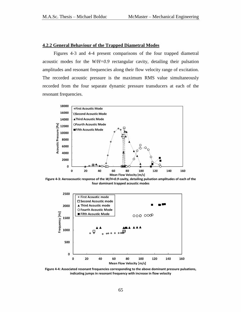
M.A.Sc. Thesis – Michael Bolduc McMaster – Mechanical Engineering
65
4.2.2 General Behaviour of the Trapped Diametral Modes
Figures 4-3 and 4-4 present comparisons of the four trapped diametral
acoustic modes for the W/H=0.9 rectangular cavity, detailing their pulsation
amplitudes and resonant frequencies along their flow velocity range of excitation.
The recorded acoustic pressure is the maximum RMS value simultaneously
recorded from the four separate dynamic pressure transducers at each of the
resonant frequencies.
Figure 4-3: Aeroacoustic response of the W/H=0.9 cavity, detailing pulsation amplitudes of each of the
four dominant trapped acoustic modes
Figure 4-4: Associated resonant frequencies corresponding to the above dominant pressure pulsations,
indicating jumps in resonant frequency with increase in flow velocity
M.A.Sc. Thesis – Michael Bolduc McMaster – Mechanical Engineering
66
As displayed in the above figures, the trapped acoustic modes are excited
along two separate flow velocity ranges. The first three modes are weakly excited
within the range of 20-40m/s and all four trapped modes are strongly excited
within the range of 50-130m/s with significantly higher pulsation amplitudes.
Along each of these velocity ranges, the frequency jumps from one acoustic mode
to the next in sequence of its defined modal number. These frequency jumps
occur with an increase in flow velocity. This behaviour is a common characteristic
found within flow-excited acoustic resonance present within cavities
(Schachenmann & Rockwell, 1982).
The two velocity ranges represent two different hydrodynamic modes of the
shear layer instability exciting the trapped acoustic modes. The free shear layer
modal number, n, designates the number of vortices (wavelengths) present along
the cavity length during an acoustic cycle. From inspection of the aeroacoustic
response, the four trapped acoustic modes are excited by the first two (n=1, 2) free
shear layer oscillation modes corresponding to one or two vortices being
convected downstream the length of the cavity. These oscillations only occur at
predefined frequencies, determined by their respective dimensionless Strouhal
number defined as:
(4.1)
where f represents the resonant frequency, L represents the cavity length
(constant at 25.4mm), and U represents the mean flow velocity. Figure 4-5
presents the Strouhal number of each of the four trapped modes during the two
velocity ranges of excitation. Likewise, Figure 4-6 presents the dimensionless
acoustic pressure of these modes at the corresponding Strouhal numbers. The
dimensionless acoustic pressure is the RMS acoustic pressure, P, normalized by
the dynamic head ( ).

M.A.Sc. Thesis – Michael Bolduc McMaster – Mechanical Engineering
67
Figure 4-5: Strouhal number as a function of the mean flow velocity during the dominant excitation of the
four trapped acoustic modes of the cavity with W/H=0.9
Figure 4-6: Dimensionless acoustic pressure of the dominant acoustic modes as a function of the Strouhal
number for the cavity with, W/H=0.9.
As clearly shown from the above plots, the two flow velocity ranges of
excitation represent two distinct ranges of Strouhal numbers. The first range,
St=0.3-0.5, corresponds to the first shear layer mode and represents the

M.A.Sc. Thesis – Michael Bolduc McMaster – Mechanical Engineering
68
propagation of one vortical structure along the cavity length. This shear layer
mode excites the trapped modes at the flow velocity range of 50-140m/s and
coincides with the very strong pressure pulsations observed in Figure 4-3. The
four trapped modes are also excited from 20-40m/s by the second shear-layer
mode, with a Strouhal number range of St=0.7-0.9. However, it generates
comparably weaker acoustic resonance as observed from the significant difference
in the maximum dimensionless acoustic pressure at the two Strouhal numbers.
These two Strouhal number ranges are consistent for all three tested cavity
geometries, as shown in a similar plot for the square cavity in Figure 4-7.
However, depending on the relative strength of each of the excited acoustic
modes, the individual Strouhal number range may slightly vary. As shown in
Figure 4-6 and 4-7, the Strouhal range of the fourth acoustic mode is significantly
larger than that of the W/H=0.9 cavity. This is due to the excitation of the fourth
mode being stronger and occurring over a longer velocity range. Nonetheless, the
onset Strouhal number for the fourth mode, corresponding to the onset excitation
velocity, remains constant for all tested cavities with a value around St=0.5.
Figure 4-7: Dimensionless acoustic pressure of the dominant acoustic modes as a function of the Strouhal
number for the square, W/H=1, cavity

M.A.Sc. Thesis – Michael Bolduc McMaster – Mechanical Engineering
69
Figures 4-8, 4-9, and 4-11 illustrate the aeroacoustic responses of the three
cavity geometries. For each of the three cases, strong acoustic resonance occurs
within the flow velocity range of 50-130m/s triggered by the first shear layer
mode. Only one trapped mode is usually excited and the switching to higher order
modes occurs abruptly. However, simultaneous excitations of the third and fourth
acoustic modes occur for all cavities in the velocity range of 80-100m/s. Within
the lower velocity range of resonance (20-40m/s), where the excitation is caused
by the second shear-layer mode, much smaller pulsation amplitudes are recorded
and the excitation of the four trapped modes tends to be intermittent.
4.2.3 Effect of Geometry on Aeroacoustic Response
In the rectangular asymmetric geometries, Figures 4-8 and 4-9, the
resonance of the second acoustic mode tends to be suppressed by the
neighbouring resonance of the first and the third acoustic modes. Although the
resonant frequencies of the first and the second modes are only slightly offset,
around 50-100Hz, the excitation of the first mode is predominant along the
majority of the velocity range from 50-80m/s. Then suddenly the second acoustic
mode rises to high pulsation amplitudes at around 11000-12000kPa before it is
soon after overcome by the excitation of the third mode.
During the switching of these acoustic modes, from 70-80m/s, only one
mode is excited at a time which is represented by the dashed lines within these
figures. This suppression effect is even more pronounced for the W/H=0.9 cavity,
Figure 4-9, where smaller velocity increments were taken in order to inspect the
resonance of the second acoustic mode.

M.A.Sc. Thesis – Michael Bolduc McMaster – Mechanical Engineering
70
Figure 4-8: Aeroacoustic response detailing the excitation of each of the trapped modes for the rectangular, W/H=0.95, cavity
Figure 4-9: Aeroacoustic response detailing the excitation of each of the trapped modes for the rectangular, W/H=0.9, cavity
At the lower velocity ranges of the cavity with W/H=0.9, (25-35m/s),
corresponding to the second shear-layer mode, the first and the second acoustic
modes are excited simultaneously. Due to only a 50-100Hz difference in resonant
frequencies, this dual excitation creates a beating phenomenon at the corner
pressure transducers at a beating frequency equal to the difference of the two

M.A.Sc. Thesis – Michael Bolduc McMaster – Mechanical Engineering
71
resonant frequencies. The normalized time signals of the beating phenomenon are
shown in Figure 4-10 for the W/H=0.9 cavity at 31m/s. This simultaneous
excitation, however, only occurs when the acoustic pressure amplitudes are quite
small, at around 500Pa, in comparison to the much stronger amplitudes, 11500Pa,
found at higher flow velocities. Due to these low excitation levels, emphasis will
be placed on the strong resonance caused by the first shear-layer mode.
Figure 4-10: Dimensionless pressure signals indicating beating at the corner pressure transducers,
W/H=0.9 cavity, 31m/s
In the case of the square cavity, Figure 4-11, the first and second orthogonal
modes are degenerate as they have the same resonant frequency. As will be
investigated within the next section, the resonance of this acoustic mode was
observed to be spinning due to the inherent symmetry present within the cavity
cross-sectional geometry. The square cavity recorded the largest pulsation
amplitudes of approximately 14500Pa from either excitation of the degenerate or
the fourth acoustic mode. Despite having similar frequencies and dimensions to
the first two modes within the rectangular cavities, the degenerate mode has a
significant increase in acoustic pressure. This increase in acoustic energy through
degeneracy was also observed by Aly through the installation and removal of a
splitter plate within an axisymmetric cavity (Aly & Ziada, 2011).

M.A.Sc. Thesis – Michael Bolduc McMaster – Mechanical Engineering
72
Figures 4-8, 4-9 and 4-11 illustrate some general trends of the excitation of
the trapped modes as the cross-sectional cavity dimensions are altered. With the
exception of the degenerate mode, the acoustic pressure amplitudes of the first
three acoustic trapped modes remain nearly constant with minor variations in the
cavity geometry. For these mode shapes, the acoustic energy is predominantly
confined within the corners of the cavity and is hardly affected with small
variations in the width. This results in only slight changes in pressure amplitudes
for the first two modes and insignificant changes in the third.
However, in the case of the fourth acoustic mode, the anti-nodes are located
at the midpoint of the cavity side lengths. As the cavity becomes smaller, through
reduction in W, the acoustic energy becomes less confined within the cavity
domain resulting in an increasingly less trapped acoustic mode. This is observed
through the large 9000Pa drop in acoustic pressure as the cavity width W is
reduced from W/H=1 to W/H=0.9. This reduction in the confinement of acoustic
energy has also been observed through comparisons of the simulated mode shapes
and acoustic particle velocity distributions previously discussed in Chapter 3.
Figure 4-11: Aeroacoustic response detailing the excitation of each of the trapped modes for the square, W/H=1, cavity

M.A.Sc. Thesis – Michael Bolduc McMaster – Mechanical Engineering
73
4.2.4 Effect on Pressure Drop
In gate valve applications, the strong excitation of the trapped diametral
modes can lead to undesirable consequences including an increase in pressure
drop across the valve, leading to lower overall plant efficiency. To investigate this
effect on the current cavity geometries, eight static pressure taps located along the
piping circumference 30cm upstream and downstream from the cavity corners
were installed to account for the asymmetric nature of the modes. Figure 4-12
presents the pressure drop across the square, W/H=1.0, cavity during its
aeroacoustic response.
As shown, the pressure drop across the cavity increases substantially during
the strong acoustic resonance of the four trapped diametral modes. Particularly
large peaks occur at 50-70m/s and 100-120m/s coinciding to excitation flow
velocities of the predominant degenerate and fourth acoustic mode shown in
Figure 4-11. This rise in pressure loss is due to the kinetic energy now being used
to sustain the large acoustic resonance of the trapped modes. This behaviour is
observed in all three cavity geometries, see Appendix A. As the cavities become
smaller, and the resonance of the trapped modes becomes weaker, the pressure
drop reduces in comparison.
Figure 4-12: Static pressure drop across the square, W/H=1.0, cavity during its aeroacoustic response

M.A.Sc. Thesis – Michael Bolduc McMaster – Mechanical Engineering
74
4.3 Upstream Flow Conditions
The upstream boundary layer for the square cavity was measured using
Laser Doppler Velocimetry (LDV). Two sets of measurements were conducted at
pre-resonance, 36.5m/s, and resonance, 61m/s, conditions at one pipe diameter
from the upstream shear layer. In both sets of measurements, the cavity centerline
turbulence intensity normalized by the mean velocity measured at the bell mouth
exit, is approximately 2.5%. Both resolved velocity profiles were flat with a
boundary layer thickness of approximately 20mm. The mean velocity profile for
the pre-resonance case, 36.5m/s, is shown in Figure 4-13 and the resonance case,
61m/s, is displayed in Figure 4-14.
Figure 4-13: Radial profile of mean flow velocity measured one pipe diameter upstream of square cavity
at pre-resonance conditions, 36.5m/s
Figure 4-14: Radial profile of mean flow velocity measured one pipe diameter upstream of square cavity at resonance conditions, 61m/s

M.A.Sc. Thesis – Michael Bolduc McMaster – Mechanical Engineering
75
4.4 Modal Behaviours
Through observations of the experimental results, three distinct behaviours
of the acoustic modes were encountered and investigated in regards to the
interaction between the resonant sound field and the downstream propagating
disturbances. These modal behaviours are classified as the following
1) Excitation of a Single Stationary Trapped Diametral Mode
2) Simultaneous Excitation of Two Stationary Modes at Separate Frequencies
3) Simultaneous Excitation of Two Equivalent Orthogonal (Degenerate) Modes
These three unique excitation mechanisms were studied through both the
experimental results and numerical simulations. First, the modal behaviours were
categorized through observations of the instantaneous time signals of each of the
four dynamic pressure transducers. Numerical simulations were then conducted to
resolve the resonant sound field and corresponding radial acoustic particle
velocity distributions. Finally, the influence of the resonant sound field on the
formation of vortical structures was investigated through two-dimensional
qualitative phase-averaged PIV (Particle Image Velocimetry).
Due to the complex interaction between the acoustic particle velocity and
the three-dimensional flow field, focus is placed on the shear layer near the cavity
upstream corner where the development and propagation of the vortical
disturbances is initiated. The following modal analysis was conducted on the
square cavity, whose response is shown in Figure 4-11. This geometry was chosen
due to the existence of all three described modal behaviours.

M.A.Sc. Thesis – Michael Bolduc McMaster – Mechanical Engineering
76
4.4.1 Excitation of a Single Stationary Trapped Diametral Mode
In most instances, the trapped acoustic modes are stationary, excited
independently, and occur at separate flow velocities. As the mean flow velocity
increases, the excited acoustic modes switch in sequence of their defined modal
number. Due to the asymmetry inherent within the rectangular geometries, each of
the first two acoustic modes has one unique mode shape, resulting in a stationary
behaviour. This is different from the degenerate acoustic mode whose behaviour
will be analyzed in Section 4.4.3.
As well, the higher order third and fourth acoustic modes are also stationary
with the corners and the midpoints of the side lengths being the only possible
orientation for their anti-nodes and nodal lines. Investigation on the independent
excitation of stationary modes is conducted on both the third and fourth acoustic
mode present within the square cavity. The fourth mode’s dimensionless acoustic
pressure and radial acoustic particle velocity distribution at the upstream cavity
corner is displayed in Figure 4-15.
Figure 4-15: Normalized acoustic pressure and radial acoustic particle velocity distribution of the fourth acoustic mode at the upstream cavity corner, W/H=1, square cavity
As shown, the radial acoustic particle velocity distribution is non-uniform
and is akin to its modal shape. The amplitude of the velocity fluctuations along
the circumference corresponds to the relative azimuthal position of the acoustic
pressure. Thus, the radial velocity fluctuations are maximum at the locations of the

M.A.Sc. Thesis – Michael Bolduc McMaster – Mechanical Engineering
77
anti-nodes and zero at the nodal lines. This separates the radial particle velocity
fluctuations into four circumferential sections. This varying azimuthal distribution
causes a non-uniform triggering of the shear layer and development of vortical
structures.
To investigate this non-uniform formation and propagation of disturbances,
two-dimensional qualitative PIV was utilized. Due to the flow field and particle
velocity distribution being highly three-dimensional along the shear layer
circumference, four sections along the shear layer were investigated. These
domains are physically separated by 90˚, and the field of view projections are
represented by the dashed lines in Figure 4-16 (left). The projection of the 0˚
domain along the cavity length is shown in Figure 4-16 (right) as an example.
This projection technique is exercised for the remaining PIV measurements within
this chapter.
Figure 4-16: Schematic illustrating the four projected measurement domains and their respective field-of-view for PIV flow visualization. Phase-averaging through all tests was done through triggering by pressure
transducers PT2 and PT3
In regards to the fourth acoustic mode, the four projected measurement
domains coincide with the maximum radial acoustic particle velocity fluctuations.
Those domains physically separated by an angle of 180˚ are in phase (with the

M.A.Sc. Thesis – Michael Bolduc McMaster – Mechanical Engineering
78
same velocity fluctuation amplitude and radial direction) and those domains that
are orthogonal are completely out of phase (same fluctuation amplitudes but in
opposite radial directions).
The PIV measurements, Figure 4-17, consist of phase-averaging 250
instantaneous vorticity fields at 90˚ temporal phase shifts, ϕ, along the fourth
mode’s acoustic cycle. Synchronization and triggering of the PIV was done via
the instantaneous time signal of pressure transducer PT2. Measurements were
conducted at a mean flow velocity of 104m/s and at the fourth mode’s resonant
frequency of 1480Hz. The four projected measurement domains are labelled by
their defined physical angle (0˚, 90˚, 180˚, and 270˚) and illustrate the propagation
of disturbances along the normalized cavity length (y/L) from the upstream to
downstream cavity corners.
ϕ=0˚ ϕ=180˚
ϕ=90˚ ϕ=270˚
Figure 4-17: Phase-averaged vorticity fields during the excitation of the fourth acoustic mode for four
instants during the acoustic cycle separated by 90˚ phase shifts, ϕ, f4=1480Hz, 104m/s
As illustrated by the average vorticity fields, the propagation of disturbances
are non-uniform and akin to radial acoustic particle velocity distribution detailed

M.A.Sc. Thesis – Michael Bolduc McMaster – Mechanical Engineering
79
in Figure 4-15. Those domains that are separated by a physical angle of 180˚ show
the formation of two parallel vortices which are in phase and at the same
downstream distance along the cavity length, y/L. Those planes that are
orthogonal to one another show two vortices completely out of phase by 180˚.
This latter behaviour is evident through side-by-side comparisons of the ϕ = 0˚
and 180˚ vorticity fields.
A similar analysis was conducted on the third acoustic mode whose mode
shape and radial acoustic particle velocity distributions are shown in Figure 4-18.
Once again, the radial acoustic particle velocity distribution is akin to the acoustic
pressure, with the anti-nodes corresponding to the maximum radial velocity
fluctuations. The same four PIV measurement domains were used; however, these
measurement locations now coincide within the nodes, where the radial acoustic
particle velocity fluctuations are zero.
Figure 4-18: Normalized acoustic pressure and radial acoustic particle velocity distribution of the third
acoustic mode at the upstream cavity corner, W/H=1, square cavity
Phase-averaged PIV was conducted at four separate temporal phase shifts,
ϕ, separated by 90˚ along the third mode’s acoustic cycle. Measurements were
synchronized and triggered off the corner dynamic pressure transducer PT3 which
is situated within the anti-node of the third mode. The measurements are
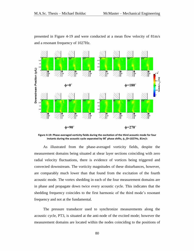
M.A.Sc. Thesis – Michael Bolduc McMaster – Mechanical Engineering
80
presented in Figure 4-19 and were conducted at a mean flow velocity of 81m/s
and a resonant frequency of 1027Hz.
ϕ=0˚ ϕ=180˚
ϕ=90˚ ϕ=270˚
Figure 4-19: Phase-averaged vorticity fields during the excitation of the third acoustic mode for four
instants during the acoustic cycle separated by 90˚ phase shifts, ϕ, f3=1027Hz, 81m/s
As illustrated from the phase-averaged vorticity fields, despite the
measurement domains being situated at shear layer sections coinciding with zero
radial velocity fluctuations, there is evidence of vortices being triggered and
convected downstream. The vorticity magnitudes of these disturbances, however,
are comparably much lower than that found from the excitation of the fourth
acoustic mode. The vortex shedding in each of the four measurement domains are
in phase and propagate down twice every acoustic cycle. This indicates that the
shedding frequency coincides to the first harmonic of the third mode’s resonant
frequency and not at the fundamental.
The pressure transducer used to synchronize measurements along the
acoustic cycle, PT3, is situated at the anti-node of the excited mode; however the
measurement domains are located within the nodes coinciding to the positions of

M.A.Sc. Thesis – Michael Bolduc McMaster – Mechanical Engineering
81
pressure transducers PT1 and PT2. The acoustic spectra of PT2 and PT3 are
shown in Figure 4-20. As expected, PT3 is dominated by the large pulsation
amplitudes at the resonant frequency, f3=1027Hz. However, PT2’s prevailing
component is the first harmonic, 2f3=2054Hz.
Figure 4-20: Acoustic spectra of pressure transducer PT2 and PT3 during the excitation of the third acoustic mode, 81m/s
This prevailing behaviour of the harmonic frequency is due to nonlinear
effects becoming significant during the strong excitation of the acoustic modes.
Although the fundamental frequency becomes insignificant at the node, the
harmonic component is still prominent. This causes the shear layer at the node,
being influenced by the acoustic pressure, to now being excited at the harmonic
frequency initiating the formation of downstream propagating disturbances at
twice the resonant frequency. Observations of the instantaneous time signals
verify that the pressure signals of PT1 and PT2 are completely in phase,
consistent to the in-phase formation and propagation of vortices in each of the
four measurement domains. A similar behaviour is observed from the independent
excitation of the fourth acoustic mode where the pressure transducer signals in the
corner, located within the nodes, are dominated by the first harmonic frequency.
PT2
PT3

M.A.Sc. Thesis – Michael Bolduc McMaster – Mechanical Engineering
82
From observations of the previous two cases, the non-uniform radial
acoustic particle velocity distribution results in a complex three-dimensional
triggering of vortical structures along the shear layer circumference. The strong
excitations of these trapped acoustic modes prove that a uniform synchronized
excitation over the whole shear layer circumference is not necessary to maintain
orderly and coherent vortical structures that sustain strong flow-acoustic coupling
and produce strong acoustic resonance exceeding 170dB.
4.4.2 Simultaneous Excitation of Two Modes at Separate Frequencies
In the flow velocity range of 80-100m/s, simultaneous excitation of the third
and fourth trapped acoustic modes is observed for all three tested cavities. Time
averaged spectra at 92m/s for the W/H=1 square cavity, Figure 4-21, shows
comparable pulsation amplitudes of each of the two excited acoustic modes.
Figure 4-21: Time averaged acoustic spectra of the four pressure transducers during simultaneous excitation of the third and fourth acoustic mode for the square cavity at 92m/s
As observed from the relative amplitudes of the spectral peaks, the four
dynamic pressure transducers are measuring different amplitudes of the third and

M.A.Sc. Thesis – Michael Bolduc McMaster – Mechanical Engineering
83
fourth acoustic modes depending on their measuring position in the mode shape.
The first two pressure transducers, PT1 & PT2, located at the middle of the
sidewalls, are measuring the maximum amplitude of the fourth acoustic mode,
f4=1490 Hz, while sensing negligible pressure amplitudes of the third acoustic
mode, f3 = 1033 Hz. This is because they are located at the anti-nodes of the fourth
mode and the nodes of the third mode. Similarly the third and fourth transducers,
PT 3 & PT4, are measuring the third acoustic mode with negligible amplitudes of
the fourth. Normalized instantaneous time signals corresponding to the acoustic
spectra are presented in Figures 4-22 for PT2 and Figure 4-23 for PT3.
Figure 4-22: Instantaneous time signal of PT 2, depicting sinusoidal oscillations at f4=1480Hz
Figure 4-23: Instantaneous time signal of PT 3, depicting sinusoidal oscillations at f3=1033Hz

M.A.Sc. Thesis – Michael Bolduc McMaster – Mechanical Engineering
84
The two time signals in the previous figures are recorded simultaneously
and are both normalized by the maximum recorded pressure from Figure 4-23.
As illustrated from the spectra, the two pressure signals have comparable
amplitudes and consist of a combination of the resonant frequencies and
harmonics of the two excited modes as depicted by their complex and nonlinear
signals. Nonetheless, the dominant sinusoidal component is the resonant
frequency of the fourth mode for PT 2 and the third mode for PT3. The evidence
of these pressure transducers recording different resonant frequencies at the same
instant illustrates that these modes are not switching but rather excited
concurrently. This behaviour suggests that the shear layer is able sustain the
excitation of multiple modes simultaneously.
The normalized acoustic pressure and radial acoustic particle velocity
distribution of the two simultaneously excited acoustic modes are shown in Figure
4-24. As discussed previously, the radial acoustic particle velocity distribution is
broken down into separate circumferential sections at which the radial acoustic
particle velocity fluctuations excite the shear layer oscillations. Comparing these
two distributions shown in Figure 4-24, circumferential portions which are
exposed to high acoustic particle velocity fluctuations by the third acoustic mode
are exposed to significantly smaller radial velocity fluctuations from the fourth
mode, and vice versa.

M.A.Sc. Thesis – Michael Bolduc McMaster – Mechanical Engineering
85
Figure 4-24: Dimensionless acoustic pressure and radial acoustic particle velocity distributions for the simultaneous excitation of the third and fourth acoustic mode
This dual excitation mechanism suggests that not only specific
circumferential portions of the shear layer are oscillating, but separate portions are
oscillating independently and at distinct resonant frequencies. This creates a very
complex excitation mechanism, consisting of eight separate circumferential
sections whose neighboring portions are oscillating at different frequencies. Those
portions, whose locations correspond within the corner of the cavity, are
oscillating independently at the resonant frequency of the third acoustic mode, f3,
and those within the side length correspond to oscillations at f4.
To investigate the flow structures coexisting from the simultaneous dual
excitation, PIV measurements were conducted using the same four measurement
domains and pressure transducers from the preceding cases involving independent
excitation. Due to the complexity of the acoustic signals, a band-pass Butterworth
filter was utilized to extract each resonant frequency for phase averaging. Two
sets of phase-averaged measurements, corresponding to each of the two

M.A.Sc. Thesis – Michael Bolduc McMaster – Mechanical Engineering
86
simultaneously excited modes, were conducted at a flow velocity of 91m/s where
the pulsation amplitudes of the two modes were comparable. Figure 4-25 presents
the average resolved vorticity fields due to phase-locking off the fourth mode’s
resonant frequency using PT2 located below. These measurements were
conducted at four equal interval phase shifts, ϕ, separated by 90˚ along the fourth
mode’s resonant cycle at f4=1484Hz.
ϕ=0˚ ϕ=180˚
ϕ=90˚ ϕ=270˚
Figure 4-25: Phase-averaged vorticity fields during dual excitation corresponding to the fourth acoustic
mode taken at four instants of the fourth mode acoustic cycle separated by 90˚ phase shifts, ϕ,
f4=1484Hz, 91m/s
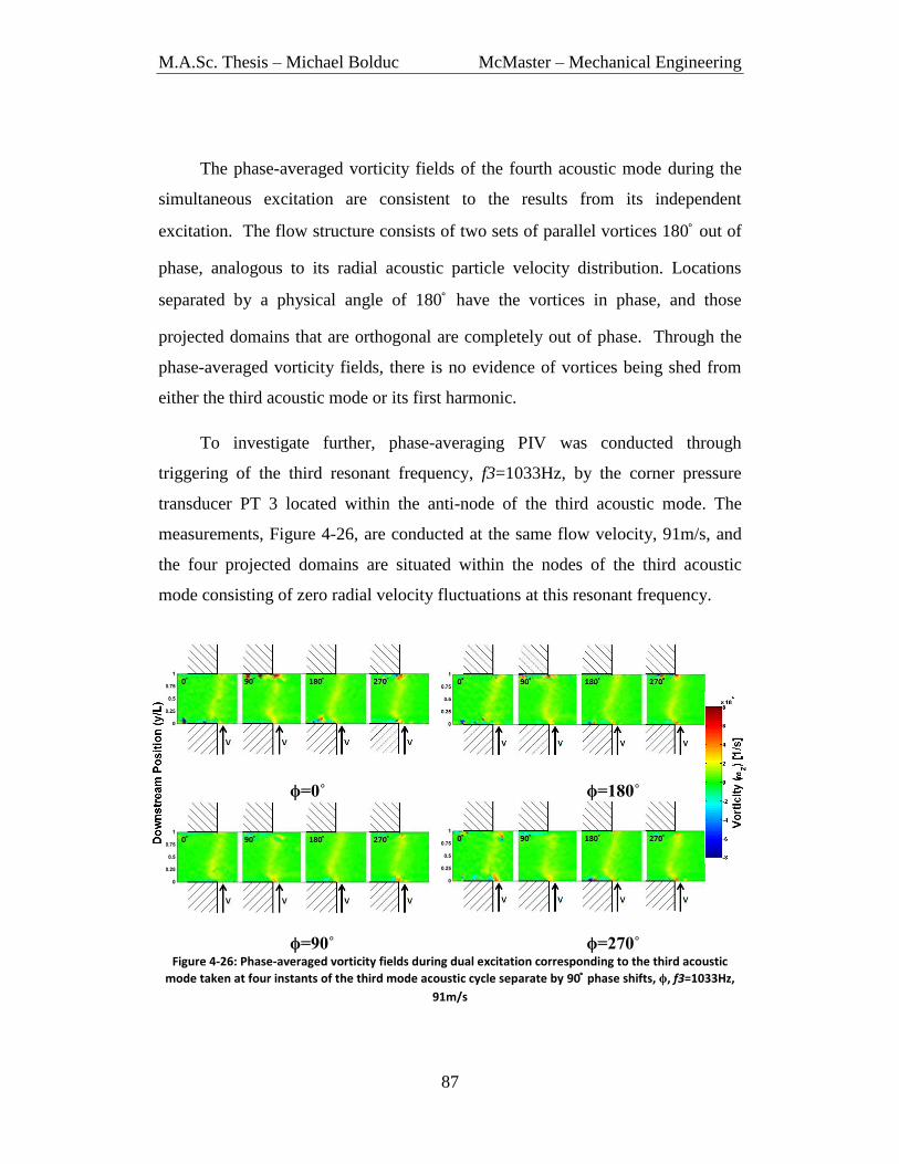
M.A.Sc. Thesis – Michael Bolduc McMaster – Mechanical Engineering
87
The phase-averaged vorticity fields of the fourth acoustic mode during the
simultaneous excitation are consistent to the results from its independent
excitation. The flow structure consists of two sets of parallel vortices 180˚ out of
phase, analogous to its radial acoustic particle velocity distribution. Locations
separated by a physical angle of 180˚ have the vortices in phase, and those
projected domains that are orthogonal are completely out of phase. Through the
phase-averaged vorticity fields, there is no evidence of vortices being shed from
either the third acoustic mode or its first harmonic.
To investigate further, phase-averaging PIV was conducted through
triggering of the third resonant frequency, f3=1033Hz, by the corner pressure
transducer PT 3 located within the anti-node of the third acoustic mode. The
measurements, Figure 4-26, are conducted at the same flow velocity, 91m/s, and
the four projected domains are situated within the nodes of the third acoustic
mode consisting of zero radial velocity fluctuations at this resonant frequency.
ϕ=0˚ ϕ=180˚
ϕ=90˚ ϕ=270˚ Figure 4-26: Phase-averaged vorticity fields during dual excitation corresponding to the third acoustic
mode taken at four instants of the third mode acoustic cycle separate by 90˚ phase shifts, ϕ, f3=1033Hz,
91m/s

M.A.Sc. Thesis – Michael Bolduc McMaster – Mechanical Engineering
88
As shown in Figure 4-26, the vorticity fields are identical at each of the
separate phase shifts. There are no coherent structures corresponding to the third
resonant frequency or its harmonic. Despite the lack of vortices being present
within the average vorticity field, each of the 250 instantaneous images consists of
two sets of parallel vortices due to the simultaneous excitation of the fourth
acoustic mode. One such instantaneous vorticity field is displayed in Figure 4-27.
Once phase-averaged, shown in Figure 4-26, the phase-averaged vorticity field is
smoothed out into the distributed paths which the fourth mode vortices are
convected along the cavity length. This is due to the fact that the locations of the
vortices differ in each of the 250 instantaneous images.
Figure 4-27: Instantaneous vorticity field through phase-triggering long the third mode’s acoustic cycle illustrating a pair of vortices from the simultaneous excitation of the fourth mode
In these two sets of measurements, the four projected domains coincide to
the large velocity fluctuations of the fourth mode and the nodal lines of the third.
The formation of vortices occurred predominantly at the fourth mode’s resonant
frequency consistent to the results of its independent excitation. The simultaneous
excitation of the third acoustic mode, however, had no effect on the initiation of
disturbances, despite it having comparable pulsation amplitudes. If measurements
were conducted within the corners of the cavity, coinciding to the maximum
fluctuations of the third acoustic mode and the nodal lines of the fourth, the
opposite behaviour would be expected. The four circumferential shear layer
sections at the cavity corners would initiate vortices at the third mode’s resonant
frequency with negligible influence from the simultaneous excitation of the fourth
mode.
These results verify that the independence of the circumferential portions
along the shear layer circumference allow the simultaneous excitation of multiple

M.A.Sc. Thesis – Michael Bolduc McMaster – Mechanical Engineering
89
diametral acoustic modes. The non-uniform excitation not only allows specific
circumferential portions to be excited, but neighbouring portions may oscillate
independently and initiate vortices at separate resonant frequencies concurrently.
These portions coincide to regions of significant radial velocity fluctuations akin
to its acoustic mode shape. Despite this convoluted radial acoustic particle
velocity distribution, the flow structures along the shear layer are coherent
allowing the strong excitation of both acoustic modes simultaneously.
In the cases of the rectangular cavities, W/H 1, the first and second
acoustic modes were only excited independently and at separate flow velocities
despite the dimensions varying slightly off unity, W/H=0.9-0.95, and having
similar natural frequencies and onset resonance velocities. An explanation of this
behaviour may be observed through comparisons of their radial acoustic particle
velocity distributions along the circumference of the upstream cavity corner.
These distributions of the W/H=0.9 cavity are displayed in Figure 4-28.
Figure 4-28: Acoustic mode shapes and radial particle velocity distributions of the first two acoustic
modes, W/H=0.9 cavity
Unlike the previous case involving excitation of the third and the fourth
acoustic modes, the regions of the maximum radial acoustic particle velocity are

M.A.Sc. Thesis – Michael Bolduc McMaster – Mechanical Engineering
90
not located within the nodes of the other excited acoustic mode. Instead, both
acoustic modes have strong radial velocity fluctuations at the corners of the
cavity. These fluctuations are expected to force the shear layer to oscillate at two
separate frequencies. This may suppress any coherent oscillations of the shear
layer. The preferential excitation of one mode over another may be due to acoustic
energy being more trapped for the first acoustic mode than the second. This is
because the energy is situated at larger radial distances from the attached piping.
4.4.3 Simultaneous Excitation of Two Degenerate Modes
The presence of asymmetry inherent within the rectangular cavities ensured
that there is one unique modal shape for each trapped acoustic mode and its
resonant frequency. This led to a stationary behaviour where the anti-nodes and
nodal lines would remain fixed and situated to those locations resolved from the
numerical simulations. With the introduction of symmetry, such as an
axisymmetric or square cavity, the preferential orientation of the acoustic mode is
now removed leading to multiple potential mode shapes that can only be satisfied
through a spinning behaviour.
This is specifically observed during the excitation of the two degenerate
modes within the square cavity. Due to the cavity cross-sectional dimensions
being equivalent, two orthogonal mode shapes were resolved for the same
resonant frequency. Hence the excitation of this acoustic mode shape did not
have a preferred orientation and the acoustic mode tended to spin with the
acoustic cycle representing one full rotation. Evidence of this spinning behaviour
is shown in the four instantaneous acoustic pressure signals during its excitation,
Figure 4-29. These time signals were recorded at a mean flow velocity of 63m/s
and normalized by the maximum measured amplitude located within the corners.
The field of view and the locations of the installed pressure transducers are
labelled.

M.A.Sc. Thesis – Michael Bolduc McMaster – Mechanical Engineering
91
Figure 4-29: Instantaneous time signal illustrating the spinning behaviour of the degenerate mode for the square cavity, 63m/s
The spinning behaviour is confirmed through the relative phase angles of
the acoustic pressure signals being equivalent to the physical enclosed angle of
the measuring pressure transducers. For example, the pressure signals of the first
and third transducers are 45˚ out of phase, equal to its separation angle, and those
of the first and second are 90˚ out of phase, which is similar to the physical angle
between the transducers. This is consistent to the definition of a fully spinning
mode rotating in the counter-clockwise direction. However, the acoustic pressure
amplitude is maximum within the corners of the cavity where the acoustic energy
is trapped and localized further away from the pipe centerline. This is indicated by
the larger recorded pressure amplitudes measured from PT3 and PT4.

M.A.Sc. Thesis – Michael Bolduc McMaster – Mechanical Engineering
92
At large pressure amplitudes associated with higher flow velocities, the
direction of spin for the acoustic mode remained fairly stabilized in the counter-
clockwise orientation as displayed in Figure 4-29. However, at lower flow
velocities and pulsation amplitudes the direction of spin became intermittent and
would vary randomly. For example, at 50m/s the mode was observed to be
spinning counter-clockwise for 20s then switched to the clockwise direction for
8s.
To illustrate the modal shape and radial acoustic particle velocity
distribution throughout the spinning mode’s acoustic cycle, the two orthogonal
mode model previously applied by Aly (2008) and Selle et al. (2006) was utilized.
This model represents the spinning behaviour through super positioning two equal
amplitude orthogonal stationary modes with a 90˚ temporal phase shift. The two
orthogonal modes were the first and second trapped acoustic modes shown in
Figure 4-30. The associated acoustic pressure and radial acoustic particle velocity
distributions are normalized by the maximum magnitude along one whole cycle of
the resultant spinning mode. Once again, emphasis is placed at the upstream
cavity corner where the development of the vortical disturbances is initiated in the
shear layer by the radial acoustic particle velocity distribution.
Figure 4-30: Super positioned orthogonal modes normalized by largest amplitude within the acoustic cycle of the resultant spinning mode

M.A.Sc. Thesis – Michael Bolduc McMaster – Mechanical Engineering
93
Eight frames of the acoustic pressure at 22.5˚ equal intervals of the phase, ,
are resolved in Figure 4-31. As displayed, the acoustic mode spins at its resonant
frequency of 851Hz, completing one full rotation throughout an acoustic cycle.
The initial position corresponds to the first orthogonal mode and the phase
represents the physical angle measured in the counter-clockwise direction from
the origin. Similar to the instantaneous time signals, the maximum acoustic
pressure occurs when the nodal line is located within the corner of the cavity.
The upstream radial acoustic particle velocity distributions for each of the
eight frames are presented in Figure 4-32. The acoustic particle velocity leads the
acoustic pressure by 90˚ as indicated through comparisons of their distributions.
As clearly shown, the radial acoustic particle velocity distribution is non-uniform
and asymmetric about its nodal line. This suggests, once again, that only specific
circumferential portions of the shear layer are being excited by the radial acoustic
particle velocity fluctuations. However, due to the spinning behaviour, these
excited circumferential sections are now varying spatially throughout its acoustic
cycle. This unique excitation mechanism, now being a function of space and time,
leads to a similarly complex three-dimensional flow field of propagating
disturbances.
To investigate the flow structures associated with the spinning mode,
qualitative two-dimensional phase-averaged PIV was conducted at the projected
domains shown in Figure 4-33. The acoustic mode preferred to spin in the
counter-clockwise direction; however, some switching did occur. Therefore a
conservative 300 instantaneous flow-fields were measured at each phase to ensure
a sufficiently averaged flow field with only those flow fields corresponding to the
counter-clockwise direction were averaged. The phase-averaged vorticity fields,
separated by a phase of 45˚, are presented in Figure 4-34. Measurements were
conducted at a mean flow velocity of 59m/s and a resonant frequency of 851Hz.

M.A.Sc. Thesis – Michael Bolduc McMaster – Mechanical Engineering
94
Figure 4-31: Instantaneous normalized acoustic pressure contours of spinning degenerate mode at phase, .

M.A.Sc. Thesis – Michael Bolduc McMaster – Mechanical Engineering
95
Figure 4-32: Instantaneous normalized radial acoustic particle velocity contours of spinning degenerate mode at phase, .

M.A.Sc. Thesis – Michael Bolduc McMaster – Mechanical Engineering
96
Figure 4-33: Projected measurement domains and spinning direction for the degenerate acoustic mode
ϕ=0˚ ϕ=180˚
ϕ=45˚ ϕ=225˚
ϕ=90˚ ϕ=270˚
ϕ=135˚ ϕ=315˚
Figure 4-34: Flow visualization of phase-averaged vorticity fields displaying the helical propagation of
disturbances along the four measurement domains at separate phase angles, ϕ, of the spinning
degenerate mode, 59m/s, 851Hz. Note: The phase angles of the images do not correspond to the same phase, , from the previous Figures

M.A.Sc. Thesis – Michael Bolduc McMaster – Mechanical Engineering
97
Through comparison of each of the phase-averaged vorticity fields, the
downstream positions of the propagating disturbances are out of phase by the
angle separating their projected measurement domains. The effect of the spinning
of the acoustic mode on the flow structure is most apparent through observations
of the ϕ= 0˚ vorticity field in which the four vortices form a diagonal line in
sequence of their measurement angle.
This behaviour is consistent to the counter-clockwise rotation of the
acoustic mode and its radial acoustic particle velocity distribution. The excited
circumferential sections are now varying spatially and so too is the initiation of
the vortical structures. As displayed in Figure 4-32, the development of
disturbances occurs all along the circumference of the shear layer near the
upstream corner and not just at these four specific measurement locations. Thus,
this vortical structure is of the helical type, similar, but spinning in opposite
direction, to the smoke flow visualization illustrated in Figure 4-35 (right) taken
from the excitation of a free round jet. The helix consists of one cycle of
revolution along the cavity length and completes a revolution around the shear
layer circumference every acoustic cycle. The helical nature is due to a
combination of the spinning acoustic mode and the convective mean flow
velocity.
Figure 4-35: Smoke flow visualization of a torodial vortex (left) and helical vortex (right) from the external excitation of a free round jet (Kusek et al., 1990)

M.A.Sc. Thesis – Michael Bolduc McMaster – Mechanical Engineering
98
This structure is consistent with the numerical simulations conducted by
Selle et al. (2006), and is significantly different from the torodial structures from
the uniform excitation of longitudinal modes, Figure 4-35 (left).
Figure 4-36: Radial acoustic particle velocity distribution of the diametral modes within an axisymmetric cavity with h=25.4mm, L/h=1 (Aly & Ziada, 2010)
A similar behaviour is expected from the spinning diametral modes within
axisymmetric cavities. The radial acoustic particle velocity distributions for the
first three diametral modes are illustrated in Figure 4-36 (Aly & Ziada, 2010). As
shown, the first diametral mode is similar to the spinning acoustic mode within
the square cavity, consisting of one nodal line. As the number of nodal lines
increase, so does the number of circumferential sections that are strongly excited
by the radial acoustic particle velocity fluctuations. The amount of nodal lines
would be equivalent to the number of parallel helices propagating downstream by
the mean flow velocity. Hence, the second diametral mode would consist of two
parallel helical structures, and the third diametral mode would consist of three.

M.A.Sc. Thesis – Michael Bolduc McMaster – Mechanical Engineering
99
CHAPTER 5 CONCLUSIONS
5.1 Summary
The excitation of trapped diametral acoustic modes within rectangular
cavities was investigated experimentally and numerically. Resonance of the first
four trapped acoustic modes dominated the aeroacoustic responses of each of the
three cavity geometries. Numerical simulations indicated that as the cavity
became smaller, and more asymmetric, the trapped nature of two of the acoustic
modes decreased. This behaviour was evident within the experimental results,
where the pulsation amplitudes of the fourth acoustic mode decreased
substantially with a reduction in the cavity width, W.
The resolved acoustic mode shapes were asymmetric, corresponding to a
non-uniform radial acoustic particle velocity distribution. This is quite different
compared to the uniform excitation of longitudinal acoustic modes and its
resultant vortex ring structure. However, the associated diametral modes were
excited strongly, indicating that a uniform excitation of the shear layer is not
necessary for sustainment of strong acoustic resonance. Throughout the
experimental results, three distinct modal behaviours were observed.
The most frequent behaviour was the independent excitation of a single
stationary mode. Results illustrated that specific circumferential portions of the
shear layer were being excited by the non-uniform acoustic particle velocity
distribution, which is generated by the acoustic mode shape. The distribution of
propagating disturbances was consistent and akin to the associated radial acoustic
particle velocity distribution. Shear layer portions that had the radial particle
velocity in phase generated propagating disturbances situated at the same
downstream position throughout its acoustic cycle. Those portions that were out
of phase had the downstream position of their vortices being separated by 180˚, as

M.A.Sc. Thesis – Michael Bolduc McMaster – Mechanical Engineering
100
illustrated from comparing their phase-averaged vorticity fields. Measurements
conducted along the nodal lines, coinciding with zero radial acoustic particle
velocity, observed the presence of weak vortical structures being propagated at
the first harmonic frequency of the excited mode.
As well, evidence verified that the shear layer was able to excite two
acoustic modes with different resonant frequencies simultaneously. The
circumferential portions which are exposed to high acoustic particle velocity
fluctuations by one acoustic mode were exposed to significantly smaller velocity
fluctuations from the other, and vice versa. Thus, neighbouring portions of the
shear layer were oscillating at different frequencies and amplitudes. Phase-
averaged vorticity fields detailed that these neighbouring sections were highly
independent from one another. The propagation of vortical structures within the
anti-node was consistent with the previous independent excitation case, with the
simultaneous excitation of the one acoustic mode having no direct influence on
the other’s development of vortical structures.
In the case of the symmetric square cavity, two resolved orthogonal mode
shapes consisted of the same resonant frequency. This degenerate acoustic mode
had no preferred orientation, leading to a spinning behaviour. Similar to the
previous cases, the asymmetry of the diametral mode allowed only specific
circumferential portions of the shear layer to be excited by the radial acoustic
particle velocity. However, due to the spinning nature, these circumferential
portions are spatially spinning 90˚ out of phase with the acoustic pressure. This
led to the formation of a helical vortical structure, spinning about the shear layer
circumference once every acoustic cycle.

M.A.Sc. Thesis – Michael Bolduc McMaster – Mechanical Engineering
101
5.2 Suggestions for Future Work
From the results of the current study, recommendations are presented for
future passive suppression techniques. In previous studies, spoilers situated at the
upstream cavity corner successfully eliminated the acoustic resonance of excited
trapped diametral modes in axisymmetric cavities (Bolduc et al., 2014). However,
these modifications introduced a significant amount of pressure drop which is
highly undesirable in the application of isolation gate valves. Since the diametral
modes were spinning within the axisymmetric cavity, the spoilers were installed
all along the circumference of the upstream cavity corner.
In the case of gate valves/rectangular cavities the diametral acoustic modes
are stationary and asymmetric. Only specific circumferential portions of the shear
layer that coincide with large acoustic particle velocity fluctuations are being
excited. Thus, spoilers would only need to be present along those shear layer
sections to eliminate the acoustic resonance. This would reduce the pressure drop
significantly in comparison to the installation along the whole shear layer
circumference.
As well, varying the number of circumferential portions that consist of
spoilers and observing the effects on the overall strength of excitation of the
acoustic mode and corresponding increase in pressure drop should prove
beneficial. If a sufficient reduction in acoustic pressure is achieved without
placing the spoilers in all the circumferential sections, then additional spoilers are
not necessary and pressure drop would be reduced. Nonetheless, the
characteristics of the acoustic mode shape and its acoustic particle velocity
distribution would need to be known in order to position these modifications
effectively.

M.A.Sc. Thesis – Michael Bolduc McMaster – Mechanical Engineering
102
REFERENCES
Aly, K. M. A. (2008). Aerodynamic excitation of the diametral modes of an
internal axisymmetric cavity (Doctoral dissertation). Hamilton, Ontario,
Canada: McMaster University.
Aly, K., & Ziada, S. (2010). Flow-excited resonance of trapped modes of ducted
shallow cavities. Journal of Fluids and Structures, 26(1), 92-120.
Aly, K., & Ziada, S. (2011). Azimuthal behaviour of flow-excited diametral
modes of internal shallow cavities. Journal of Sound and Vibration,
330(15), 3666-3683.
Aly, K., & Ziada, S. (2012). Effect of mean flow on the trapped modes of internal
cavities. Journal of Fluids and Structures, 33, 70-84.
Barannyk, O., & Oshkai, P. (2014). Investigation of diametral acoustic modes in a
model of a steam control gate valve. Journal of Pressure Vessel Technology,
136(6), 061302.
Betts, P. L. (1972). Self-induced oscillations in an open water-channel with
slotted walls. Journal of Fluid Mechanics, 55(03), 401-417.
Bolduc, M., Elsayed, M., & Ziada, S. (2014). Passive Control of Trapped Mode
Resonance of Ducted Cavities. Journal of Pressure Vessel Technology,
136(5), 051311.
Bruggeman, J. C., Hirschberg, A., Van Dongen, M. E. H., Wijnands, A. P. J., &
Gorter, J. (1991). Self-sustained aero-acoustic pulsations in gas transport
systems: experimental study of the influence of closed side branches.
Journal of Sound and Vibration, 150(3), 371-393.
Cattafesta, L., Williams, D., Rowley, C., & Alvi, F. (2003). Review of active
control of flow-induced cavity resonance. AIAA paper, 3567, 2003.
Chevray R. (1984). Entrainment in turbulent flows: mechanisms and implications
North-Holland: Elsevier Science Publishers B.V., 365-369.
Duan, Y., Koch, W., Linton, C. M., & McIver, M. (2007). Complex resonances
and trapped modes in ducted domains. Journal of Fluid Mechanics, 571,
119-147.

M.A.Sc. Thesis – Michael Bolduc McMaster – Mechanical Engineering
103
Durst, F. (1976). Principles and practice of laser-doppler aneometry. Academic
Press Inc.
Evans, D. V., & Linton, C. M. (1991). Trapped modes in open channels. Journal
of Fluid Mechanics, 225, 153-175.
Evans, D. V., Levitin, M., & Vassiliev, D. (1994). Existence theorems for trapped
modes. Journal of Fluid Mechanics, 261, 21-31.
Freymuth, P. (1966). On transition in a separated laminar boundary layer. Journal
of Fluid Mechanics, 25(04), 683-704.
Hein, S., & Koch, W. (2008). Acoustic resonances and trapped modes in pipes
and tunnels. Journal of Fluid Mechanics, 605, 401-428.
Heller, H. H., & Bliss, D. B. (1975). The physical mechanism of flow-induced
pressure fluctuations in cavities and concepts for their suppression. AIAA
paper, 491, 1975.
Ho, C. M., & Huang, L. S. (1982). Subharmonics and vortex merging in mixing
layers. Journal of Fluid Mechanics, 119, 443-473.
Hourigan, K., Welsh, M. C., Thompson, M. C., & Stokes, A. N. (1990).
Aerodynamic sources of acoustic resonance in a duct with baffles. Journal
of Fluids and Structures, 4(4), 345-370.
Howe, M. S. (1980). The dissipation of sound at an edge. Journal of Sound and
Vibration, 70(3), 407-411.
Huang, X. Y., & Weaver, D. S. (1991). On the active control of shear layer
oscillations across a cavity in the presence of pipeline acoustic resonance.
Journal of Fluids and Structures, 5(2), 207-219.
Karadogan, H., & Rockwell, D. (1983). Toward attenuation of self-sustained
oscillations of a turbulent jet through a cavity. Journal of fluids engineering,
105(3), 335-340.
Keller, J. J., & Escudier, M. P. (1983). Flow-excited resonances in covered
cavities. Journal of Sound and Vibration, 86(2), 199-226.
Kinsler, L.E., Frey, A.R., Coppens, A.B. & Sanders, J.V. (2000). Fundamentals of
Acoustics. New York: John Wiley & Sons, Inc.

M.A.Sc. Thesis – Michael Bolduc McMaster – Mechanical Engineering
104
Kline, S. J., & McClintock, F. A. (1953). Describing uncertainties in single-
sample experiments. Mechanical engineering, 75(1), 3-8.
Knotts, B. D., & Selamet, A. (2003). Suppression of flow–acoustic coupling in
sidebranch ducts by interface modification. Journal of Sound and Vibration,
265(5), 1025-1045.
Kusek, S. M., Corke, T. C., & Reisenthel, P. (1990). Seeding of helical modes in
the initial region of an axisymmetric jet. Experiments in Fluids, 10(2-3),
116-124.
Lacombe, R., Lafon, P., Daude, F., Crouzet, F., Bailly, C., & Ziada, S. (2013).
Numerical and experimental analysis of flow-acoustic interactions in an
industrial gate valve. 19th
AIAA/CEAS Aeroacoustics Conference, May27-
29, 2013 Berlin, Germany.
Lafon, P., Caillaud, S., Devos, J. P., & Lambert, C. (2003). Aeroacoustical
coupling in a ducted shallow cavity and fluid/structure effects on a steam
line. Journal of Fluids and structures, 18(6), 695-713.
Michalke, A. (1964). On the inviscid instability of the hyperbolic tangent velocity
profile. Journal of Fluid Mechanics, 19(04), 543-556.
Michalke, A. (1965). On spatially growing disturbances in an inviscid shear layer.
Journal of Fluid Mechanics, 23(03), 521-544.
Miksad, R. W. (1972). Experiments on the nonlinear stages of free-shear-layer
transition. Journal of Fluid Mechanics, 56(04), 695-719.
Mohamed, S., & Ziada, S. (2014, July). PIV Measurements of Aeroacoustic
Sources of a Shallow Cavity in a Pipeline. In ASME 2014 Pressure Vessels
and Piping Conference. American Society of Mechanical Engineers.
Morse, P. (1948). Vibration and Sound, McGraw-Hill Book Company Inc.
akibo lu, G., & Hirschberg, A. (2010, January). A numerical study of the
aeroacoustic interaction of a cavity with a confined flow: effect of edge
geometry in corrugated pipes. In ASME 2010 3rd Joint US-European Fluids
Engineering Summer Meeting collocated with 8th International Conference
on Nanochannels, Microchannels, and Minichannels (pp. 767-773).
American Society of Mechanical Engineers.
M.A.Sc. Thesis – Michael Bolduc McMaster – Mechanical Engineering
105
NRC. (2002). Failure of Steam Dryer Cover Plate after a Recent Power Uprate.
NRC Information Notice 2002-26. US Nuclear Regulatory Commission,
Washington, D.C.
O'Connor, J., Acharya, V., & Lieuwen, T. (2015). Transverse combustion
instabilities: Acoustic, fluid mechanic, and flame processes. Progress in
Energy and Combustion Science, 49, 1-39.
Rayleigh, L., (1880). On the instability or instability of certain fluid motions.
Proc. London Math. Soc, 11, 57-70.
Rockwell, D. (1983). Oscillations of impinging shear layers. AIAA journal, 21(5),
645-664.
Rockwell, D., & Naudascher, E. (1978). Review—self-sustaining oscillations of
flow past cavities. Journal of Fluids Engineering, 100(2), 152-165.
Rockwell, D., & Schachenmann, A. (1982). The organized shear layer due to
oscillations of a turbulent jet through an axisymmetric cavity. Journal of
Sound and Vibration, 85(3), 371-382.
Rossiter, J. E. (1964). Wind tunnel experiments on the flow over rectangular
cavities at subsonic and transonic speeds. Ministry of Aviation; Royal
Aircraft Establishment; RAE Farnborough.
Selle, L., Lartigue, G., Poinsot, T., Koch, R., Schildmacher, K. U., Krebs, W.,
Prade, B., Kaufmann, P., & Veynante, D. (2004). Compressible large eddy
simulation of turbulent combustion in complex geometry on unstructured
meshes. Combustion and Flame, 137(4), 489-505.
Selle, L., Benoit, L., Poinsot, T., Nicoud, F., & Krebs, W. (2006). Joint use of
compressible large-eddy simulation and Helmholtz solvers for the analysis
of rotating modes in an industrial swirled burner. Combustion and Flame,
145(1), 194-205.
Smith, B. A., & Luloff, B. V. (2000). The effect of seat geometry on gate valve
noise. Journal of pressure vessel technology, 122(4), 401-407.
Tam, C. K., & Block, P. J. (1978). On the tones and pressure oscillations induced
by flow over rectangular cavities. Journal of Fluid Mechanics, 89(02), 373-
399.
Tam, C. K. (1976). The acoustic modes of a two-dimensional rectangular cavity.
Journal of Sound and Vibration, 49(3), 353-364.

M.A.Sc. Thesis – Michael Bolduc McMaster – Mechanical Engineering
106
Tollmien, W. (1935). A General Criterion for the Instability of Laminar Velocity
Distributions
Tyler, J. M., & Sofrin, T. G. (1962). Axial flow compressor noise studies (No.
620532). SAE Technical Paper.
Worth, N. A , & Dawson, J. R.(2015). The effect of baffles on self-excited
azimuthal modes in an annular combustor. Proceedings of the Combustion
Institute, 35(3), 3283-3290.
Worth, N. A., & Dawson, J. R. (2013). Modal dynamics of self-excited azimuthal
instabilities in an annular combustion chamber. Combustion and Flame,
160(11), 2476-2489.
Ziada, S. (2010). Flow-excited acoustic resonance in industry. Journal of Pressure
Vessel Technology, 132(1), 015001.
Ziada, S., Bühlmann, E. T., & Bolleter, U. (1989). Flow impingement as an
excitation source in control valves. Journal of Fluids and Structures, 3(5),
529-549.
Ziada, S., Ng, H., & Blake, C. E. (2003). Flow excited resonance of a confined
shallow cavity in low Mach number flow and its control. Journal of fluids
and structures, 18(1), 79-92.

M.A.Sc. Thesis – Michael Bolduc McMaster – Mechanical Engineering
107
APPENDIX A ADDITIONAL RESULTS
Figure A-1: Comparison of dimensionless radial particle velocity distribution for the first acoustic mode as
a function of angle, ∅, upstream cavity corner of the three cavity geometries

M.A.Sc. Thesis – Michael Bolduc McMaster – Mechanical Engineering
108
Figure A-2: Dimensionless Acoustic Particle velocity distributions of the four acoustic modes for the Top: W/H=1, Middle: W/H=0.95, Bottom: W/H=0.9, cavities

M.A.Sc. Thesis – Michael Bolduc McMaster – Mechanical Engineering
109
Figure A-3: SPL contour plot of the aeroacoustic response for the Top=W/H=1, Middle=W/H=0.95, Bottom=W/H=0.9 cavities

M.A.Sc. Thesis – Michael Bolduc McMaster – Mechanical Engineering
110
Figure A-4: Frequency [Hz] vs. Mean Flow Velocity [m/s] Top=W/H=1, Middle=W/H=0.95, Bottom=W/H=0.9 cavities

M.A.Sc. Thesis – Michael Bolduc McMaster – Mechanical Engineering
111
Figure A-5: Strouhal Number vs. Mean Flow Velocity [m/s] Top=W/H=1, Middle=W/H=0.95, Bottom=W/H=0.9 cavities

M.A.Sc. Thesis – Michael Bolduc McMaster – Mechanical Engineering
112
Figure A-6: Dimensionless Acoustic Pressure vs. Strouhal Number Top=W/H=1, Middle=W/H=0.95, Bottom=W/H=0.9 cavities

M.A.Sc. Thesis – Michael Bolduc McMaster – Mechanical Engineering
113
Figure A-7: Pressure drop for the rectangular cavity with W/H=0.95

M.A.Sc. Thesis – Michael Bolduc McMaster – Mechanical Engineering
114
Figure A-8: Pressure drop for the rectangular cavity with W/H=0.90

M.A.Sc. Thesis – Michael Bolduc McMaster – Mechanical Engineering
115
APPENDIX B UNCERTAINTY ANALYSIS
Acoustic Measurements
The frequency and recorded acoustic pressure of the strongly excited
acoustic modes remained constant throughout their averaging. The acoustic
measurements were obtained with a National Instruments NI-9233 data
acquisition card accompanied with an anti-aliasing filter. As previously discussed,
the excitation of the acoustic modes was found to be intermittent only at low flow
velocities. To account for the intermittency, a sampling rate of 25kHz consisting
of a conservative average of fifty, 1 second long, samples with a final resolution
of =±1Hz was utilized. Those measurements taken during the strong tonal
excitation from the first shear layer mode had little influence from varying the
number of samples that were averaged.
The uncertainty in the acoustic pressure measurement is due to the
uncertainty in the calibration of the pressure transducers, 4%, the uncertainty in
the repeatability of the acoustic pressure measurements is found to be around
5.2%, and the resolution of the pressure transducers around 4.8%. To account
for these associated uncertainties, the quadratic sum method, detailed below in
equation B-1, was utilized obtaining an uncertainty in acoustic pressure of 8.0%.
(B-1)
Mean Flow Velocity
The uncertainty propagation of random uncertainties was resolved through
the method proposed by Kline & McClintock (1953), Equation B-2. is the

M.A.Sc. Thesis – Michael Bolduc McMaster – Mechanical Engineering
116
uncertainty of the dependent variable and represents the uncertainty of the
separate associated independent variables.
(B-2)
The mean flow velocity was measured through a pitot-tube situated at the
bell-mouth. The dynamic pressure was recorded using a differential pressure
transducer calibrated with a Crystal pressure calibrator with a resolution accuracy
of ±5Pa, leading to an uncertainty of . Utilizing Kline and McClintock’s
method, Equation B-3 is obtained. Thus, the mean flow velocity uncertainty
through calibration is around 1.0%
(B-3)
The relative standard deviation (RSD),
, in response of average reading of
the pitot tube was found to be around 1.0%. Thus, the overall uncertainty of the
mean flow velocity is around 1.5%
Dimensionless Numbers
From Kline and McClintock’s method, the uncertainty of dimensionless
parameters utilized within this study is evaluated. First, the uncertainty of the
dimensionless acoustic pressure,
, is represented as a function of both
acoustic pressure and mean flow velocity as represented in B-4.
(B-4)
(B-5)
M.A.Sc. Thesis – Michael Bolduc McMaster – Mechanical Engineering
117
It can be demonstrated that the associated uncertainty of the dimensionless
acoustic pressure may be represented as B-5. Utilizing the previous values of
acoustic pressure and mean flow velocity, the uncertainty of the dimensionless
acoustic pressure is around 8.5%.
Likewise, the uncertainty of the Strouhal Number,
may be
represented by the uncertainty of its independent variables as shown below.
(B-6)
(B-7)
Through additional measurements along the cavity perimeter, the tolerance
in the cavity length, L, was 1% .The resolution of the acoustic measurements was
=1Hz. Thus, the smallest resonant frequency, 851Hz, results in the largest
of
0.1%. This leads to an overall uncertainty of
is 1.8%.
Laser Doppler Velocimetry
Laser Doppler Velocimetry was utilized to resolve the radial velocity profile
situated one pipe diameter upstream from the cavity mouth at both resonance and
pre-resonance conditions. The measurements consisted of using a traverse with a
minimum step size of 0.00625mm. Measurements were taken at intervals as small
as 0.1mm.
The reproducibility of the measurements on the pre-resonance condition
illustrated that the coefficient of variability (
of the mean flow past the
boundary layer thickness was 1.0% through four reproduced tests. The smallest
measured distance from the wall was 1mm. Those distances closer to the wall
have significant velocity gradients and a lack of measured seeded particles.

M.A.Sc. Thesis – Michael Bolduc McMaster – Mechanical Engineering
118
Flow Visualization Uncertainty
The objective of these measurements was not to obtain a full quantitative
representation of the three-dimensional flow field, but to visualize the
downstream propagation of disturbances at specific circumferential sections along
the shear layer and compare it to the distinct acoustic modal behaviours that were
being observed. The phase-averaged measurements consisted of triggering the
PIV along the acoustic cycle of the investigated mode. The sampling frequency
was the maximum available from the NI-9233 data acquisition card at 50 kHz,
resulting in a resolution of s.
The finite resolution introduces an uncertainty through triggering at specific
phases of the acoustic cycle. The uncertainty is dependent on the resonant
frequency and the relative size of its oscillation period to the sampling rate. From
all measurements, the largest uncertainty coincides to the smallest period of the
fourth acoustic mode with a maximum deviation of 5.34˚. A conservative number
of instantaneous images, 250-300, were taken at each phase to reduce this error
through averaging.