The Advancement of Adaptive Relaying in Power Systems Protection

Brian Zachary Zaremski

Thesis submitted to the faculty of the Virginia Polytechnic Institute and State University in

partial fulfillment of the requirements for the degree of

Master of Science

In

Electrical Engineering

Jaime DeLaRee

Virgilio Centeno

Richard Conners

April 15th

, 2012

Blacksburg, VA

Keywords: Supervisory Zones, Adaptive Protection, Voltage, Current, Impedance, Rate of

Change, Fault, Loadability

Copyright 2012

Supervisory Zones of Protection

Brian Zachary Zaremski

ABSTRACT

The electrical distribution system in the United States is considered one of the most complicated

machines in existence. Electrical phenomena in such a complex system can inflict serious self-

harm. This requires damage prevention from protection schemes. Until recently, there was a

safe gap between capacity to deliver power and the demand. Therefore, these protection

schemes focused on dependability allowing the disconnection of lines, transformers, or other

devices with the purpose of isolating the faulted element. On some occasions, the disconnections

made were not necessary. The other extreme of reliability calls for security. This aspect of

reliability calls for the operation of the protective devices only for faults within the intended area

of protection. There is a tradeoff here; where a dependable protection scheme will assuredly

prevent damage, it is prone to unnecessary operation which can lead to cascading outages.

Where a secure scheme will not operate unnecessarily, it is prone to pieces of the system

becoming damaged when relays fail to operate properly. With microprocessor based relaying

schemes, a hybrid reliability focus is attainable through adaptive relaying. Adaptive relaying

describes protection schemes that adjust settings and/or logic of operations based on the

prevailing conditions of the system. These adjustments can help to avoid relay miss-operation.

Adjustments could include, but are not limited to, the logging of data for post-mortem analysis,

communication throughout the system, as well changing relay parameters. Several concepts will

be discussed, one of which will be implemented to prove the value of the new tools available.

iii

Dedication

I would like to dedicate the work of this thesis to my parents, David and Linda Zaremski, who

have set an amazing example for my siblings and me.

iv

Table of Contents Table of Figures ............................................................................................................................. v

Chapter 1: Introduction ................................................................................................................... 1

Section 1.1: Areas of Possible Improvement .............................................................................. 3

Chapter 2: Power System Review ................................................................................................... 5

Section 2.1: History .................................................................................................................... 5

Section 2.2: Generation ............................................................................................................... 6

Section 2.3: Transformers ........................................................................................................... 7

Section 2.4: Transmission, Subtransmission, and Distribution .................................................. 8

Section 2.5: Loads ....................................................................................................................... 8

Chapter 3: Adaptive Protection Schemes ..................................................................................... 10

Section 3.1: Data Mining .......................................................................................................... 10

Section 3.2: Differential Protection .......................................................................................... 11

Section 3.3: Communication ..................................................................................................... 13

Chapter 4: Transmission Level Adaptive Protection .................................................................... 15

Section 4.1: Transmission Basics ............................................................................................. 15

Section 4.2: Protection Basics................................................................................................... 17

Section 4.3: Development of Protection Schemes .................................................................... 18

Section 4.4: Distance Protection ............................................................................................... 22

Section 4.5: 2003 Northeast Blackout ...................................................................................... 25

Section 4.6: Supervisory Zone of Protection ............................................................................ 26

Chapter 5: Implementation of the Supervisory Zone of Protection .............................................. 29

Section 5.1: Hardware Implementation .................................................................................... 30

Chapter 6: Future Work and Conclusions ..................................................................................... 35

Section 6.1: R-R Dot ................................................................................................................. 35

Section 6.2: Conclusions ........................................................................................................... 36

References ..................................................................................................................................... 38

Appendix A ................................................................................................................................... 39

v

Table of Figures

Figure 1 ......................................................................................................................................... 22

Figure 2 ......................................................................................................................................... 23

Figure 3 ......................................................................................................................................... 25

Figure 4 ......................................................................................................................................... 26

Figure 5 ......................................................................................................................................... 27

Figure 6 ......................................................................................................................................... 30

Figure 7 ......................................................................................................................................... 31

Figure 8 ......................................................................................................................................... 31

Figure 9 ......................................................................................................................................... 32

Figure 10 ....................................................................................................................................... 32

Figure 11 ....................................................................................................................................... 32

Figure 12 ....................................................................................................................................... 33

1

Chapter 1: Introduction

The method of delivering energy in the form of electricity to businesses and homes across

the United States is one of the most complicated systems in existence. The first distribution of

electricity started in Manhattan in the 1880s [1]. That system grew into three large

interconnections of systems that span from coast to coast as well as across our borders with

Canada and Mexico. Initially, the infrastructure necessary to meet the peak demands of

electricity was allowed to grow without much hindrance, and there was a comfortable cushion

between what the system could deliver and what the consumers demanded. With the growth of

federal regulations and environmental considerations it has become more difficult to expand on

the capacity of the infrastructure, causing that gap to shrink. Consequently, power engineers are

forced to push the limits on the capacity of what they can deliver with the current system. This

has led to many changes in the approach of electricity distribution, specifically a paradigm shift

in the methods of protective relaying.

When describing its protective relaying, a system is often looked at in terms of its

reliability. This reliability spectrum has two extremes, dependability and security. A system is

said to be dependable if it will react for any type of fault, but may also operate inappropriately

when not needed. A system is said to be secure if it will not react inappropriately or

unnecessarily, but it may not react if there is indeed a fault. In the past, most protection

engineers tended to lean towards the dependability side of the spectrum in order to clear any

possible fault condition because in most cases there were alternative delivery paths to the

consumer [2]. The issue is that constraints on the growth of the infrastructure have led to

increased system stress, which leads to possible operation of dependable protection schemes

which may contribute to catastrophic cascading failures.

This stressed system state is what led to the blackout in the northeast in 2003. Due to a

problem that initiated in Ohio, a blackout ensued that affected an estimated 50 million customers

in Ohio, Michigan, Pennsylvania, New York, Vermont, Massachusetts, Connecticut, and New

Jersey in the United States, as well as Ontario in Canada. It took up to four days for some

customers to have their power restored in the United States, and some parts of Canada were

forced to deal with rolling blackouts for more than a week. The problem is that where

interconnecting with other systems provides mutual backup for providing power, it is possible

2

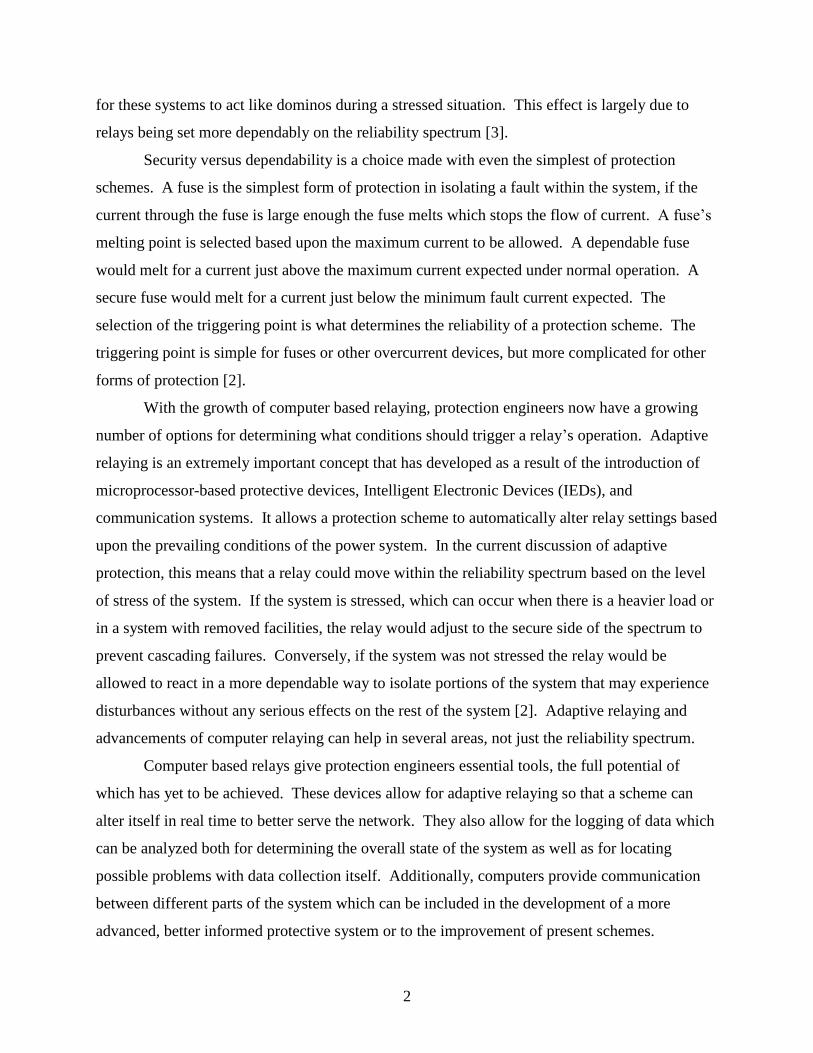
for these systems to act like dominos during a stressed situation. This effect is largely due to

relays being set more dependably on the reliability spectrum [3].

Security versus dependability is a choice made with even the simplest of protection

schemes. A fuse is the simplest form of protection in isolating a fault within the system, if the

current through the fuse is large enough the fuse melts which stops the flow of current. A fuse’s

melting point is selected based upon the maximum current to be allowed. A dependable fuse

would melt for a current just above the maximum current expected under normal operation. A

secure fuse would melt for a current just below the minimum fault current expected. The

selection of the triggering point is what determines the reliability of a protection scheme. The

triggering point is simple for fuses or other overcurrent devices, but more complicated for other

forms of protection [2].

With the growth of computer based relaying, protection engineers now have a growing

number of options for determining what conditions should trigger a relay’s operation. Adaptive

relaying is an extremely important concept that has developed as a result of the introduction of

microprocessor-based protective devices, Intelligent Electronic Devices (IEDs), and

communication systems. It allows a protection scheme to automatically alter relay settings based

upon the prevailing conditions of the power system. In the current discussion of adaptive

protection, this means that a relay could move within the reliability spectrum based on the level

of stress of the system. If the system is stressed, which can occur when there is a heavier load or

in a system with removed facilities, the relay would adjust to the secure side of the spectrum to

prevent cascading failures. Conversely, if the system was not stressed the relay would be

allowed to react in a more dependable way to isolate portions of the system that may experience

disturbances without any serious effects on the rest of the system [2]. Adaptive relaying and

advancements of computer relaying can help in several areas, not just the reliability spectrum.

Computer based relays give protection engineers essential tools, the full potential of

which has yet to be achieved. These devices allow for adaptive relaying so that a scheme can

alter itself in real time to better serve the network. They also allow for the logging of data which

can be analyzed both for determining the overall state of the system as well as for locating

possible problems with data collection itself. Additionally, computers provide communication

between different parts of the system which can be included in the development of a more

advanced, better informed protective system or to the improvement of present schemes.

3

Section 1.1: Areas of Possible Improvement

The following are just a few samples of the many possible types of protection schemes

that may benefit from computer-based adaptive relaying. Consider a differential protection

system applied to a transformer. In this protection scheme, the relay engineer will compare the

input and output currents of a transformer. Current transformers (CTs) must be carefully

selected to ensure a match of secondary currents on both sides of the transformer. Standard

values of CTs may result in discrepancies that will numerically increase with transformer

loading. A second element to consider is under-load-tap-changers (ULTC). These tap-changers

will modify the nominal turns-ratio of the transformer by adding or subtracting a small

percentage of the turns to one of the transformer sides. Once again, the discrepancy created will

be dependent on the transformer’s load. The solution to the above described problem comes in

the form of larger tolerances, which may blind the relay to small current faults. Another solution

is to implement a percentage differential scheme which is a more sophisticated and costly

protective system. Today’s technology provides us with the opportunity to consider the

mentioned limitations by allowing the micro-processor-based relay to take into consideration the

sources of errors: CT mismatch, ULTC, magnetizing currents, etc.

Hidden failure identification is another area where computer-based adaptive relaying

could prove extremely useful. A hidden failure is simply a faulty device or setting which

becomes exposed during poor operating conditions. It generally exacerbates the situation which

exposes them. With computer based relaying, these types of failures can be sought out through

data comparison and other techniques.

The main focus of this paper is to expand upon the newly developing concepts made

available by computer-based relays. In distance based protection schemes, a relay operates

based upon the apparent impedance of an operating condition as seen by the terminals of the

relay. For a given conductor size and geometry of the distribution of conductors, it is possible to

determine the impedance per unit length of a transmission line. The apparent impedance and the

impedance per unit length of the line provide the necessary information to deploy a distance

protection scheme. Also, this same information can help us identify distance protection schemes

that may be compromised as power swings and/or heavy load operating conditions may encroach

the operating characteristics of the distance relay [2].

4

During the 2003 blackout, a relay using distance protection tripped unnecessarily when

the loading of a line resulted in an encroachment into the third zone of the relay [3]. This is a

great example of an opportunity for a computer based relay to better handle relay operation. A

computer based relay can determine how quickly an operating point is moving to distinguish

between a fault and a power swing. Under a fault condition the operating point moves rapidly,

whereas a change in load causes the operating point to move slowly.

In this thesis, several of these new applications will be discussed. The next chapter will

show how the system developed into the size that it is today as well as give some background on

the different parts of the system, like generation, transmission, and loading. The third chapter

will discuss several developments in the field of adaptive protection schemes. The fourth

chapter will take an in depth look at a new concept in distance-based protection called the

supervisory zone of protection. The fifth chapter will show the implementation of this concept

using hardware and software readily available in today’s market. The last chapter will cover

possible future work on the concept, improving the scheme to focus more directly on the rate of

change of quantities being measured.

5

Chapter 2: Power System Review Section 2.1: History

The distribution of electricity in the United States of America can be traced back to

September 4th

, 1882, when Thomas Edison opened the Pearl Street Station in lower Manhattan.

Serving about a quarter of a square mile, this direct current (DC) system was primarily used for

lighting in the financial district of New York. Edison showed that it was possible to efficiently

provide electricity from a central generating station. The issue with DC systems was that the end

consumer had to be located within a few miles of the generating station. The problem was that

the low voltage used with this type of distribution led to higher currents and higher losses on the

lines used to distribute the electricity. This forced the generating plants to be small which

reduced efficiency, and it meant that only small distribution systems in densely populated areas

would be effective[1].

In distribution systems the voltage is held constant and the current flowing through the

lines depends on the load being served. The losses associated with the lines used to distribute the

electricity vary with the square of the current running through the lines. So if the current through

the lines doubles, the losses associated with the lines actually quadruples. At the time Edison

started implementing his systems, there was no way to easily change the voltage in a DC system.

The ability to vary the voltage of the distribution lines would allow for the reduction of current

during transmission, which was being developed within alternating current (AC) systems. AC

allowed for transformers to increase the voltage required by transmission and a reduction to a

voltage level that is safe for end consumers to use; this significantly reduces the losses of sending

electricity over longer distances. Nikola Tesla was the pioneer of this AC technology as well as

the concept of polyphase distribution[1].

These competing strategies of electrical distribution, AC and DC systems, led to what is

commonly known as the Battle of the Currents. Thomas Edison, owning the patents for DC

systems, argued that AC and the higher voltages associated with it was unsafe. At the same time,

however, George Westinghouse was building AC transmission lines that stretched for miles.

This, along with Nikola Tesla’s development of an AC motor among other developments, led to

the ultimate victory of AC systems. This victory of alternating current led to the electrical

distribution system we have today in which large generating stations delivering power over long

distances at high voltages, which is both economical and efficient in comparison to the original

6

DC systems [4]. This did, however, lead to several engineering issues to which solutions are still

being developed today.

The AC system pioneered by Westinghouse and Tesla has developed into one of the most

complex machines in the world. The growth started with many small independent systems. For

reliability purposes, these systems were interconnected. This interconnection of many small

systems meant that the number of machines necessary for reserve operation during peak loads

was lowered. The interconnection also enabled utility companies to get the cheapest possible

power from their neighbors. These interconnections grew into the massive system which we

have today. There are issues that arose with the creation of this massive system; these issues

include higher fault currents, cascading failures in which multiple smaller systems are affected

when the problem only occurred in one of them, and a very delicate balancing act that occurs

between systems. The planning that goes into this system, especially the protection of the

system itself, is very complicated [5]. This system is generally broken down into generation,

transmission, and loads. The transmission portion is divided into transmission, subtransmission,

and distribution; each having different voltage levels controlled using transformers. In the next

few sections, each of these topics will be explored.

Section 2.2: Generation

Generators are used to convert different forms of energy into electrical energy. Most

generators in use today convert mechanical energy into electrical energy using magnetic field

interactions. This mechanical energy is generally provided in the form of a spinning prime

mover. The prime mover usually has a magnetic field associated with it, and its spins within the

stator coils; the stator is the stationary portion of a generator, and the field on the rotor induces

currents within those stator coils. The spinning action can be provided using a steam turbine

where some source of heat boils water to drive that turbine, or in the case of a hydroelectric dam,

water could spin a turbine directly. Sometimes internal combustion engines can also be directly

coupled to a prime mover. Steam power plants generate their heat by burning coal, natural gas,

or oil as well as using nuclear reactions to generate heat. In the case of using a prime mover type

generator, the speed at which that generator spins is extremely important because it determines

the electrical output frequency. The great thing about all the types of generation discussed so far

is that their output levels can be controlled by varying the amount of energy put into the prime

movers [6].

7

Other, less controllable, forms of generation include renewables like solar and wind

power. Solar power can be in the form of photovoltaic energy which needs to be converted from

DC to AC to contribute to the system, or solar thermal which can be incorporated like any other

thermal based generation. Wind power generates electricity with a prime mover, but because

wind speeds are not constant the electricity must be conditioned using power electronics to

ensure the output has the correct voltage and frequency. The main issue with these types of

generation is that there is no way to control their output, so there isn’t any way to predict

accurately how these sources will contribute. Another issue is that when small scale projects are

implemented and feed energy back into the grid, current flow can change direction which may

affect the operation of certain types of protective relays [6]. So while it is good to have a

contribution from renewable resources, there is a tradeoff in the predictability of operation.

Section 2.3: Transformers

Transformers are an essential part of the electrical distribution system, as discussed

earlier. Generation is generally done at voltage levels between 13.8 kV and 24 kV.

Consumption of this electricity is generally done at voltage levels between 110 V in homes and

up to 4160 V in large industrial plants. Transmission of electricity can occur at levels of 115 kV

to 765 kV in the United States, and go as high as 1 megavolt in other parts of the world.

Transformers are what make this wide range of voltage level capabilities possible. Without

transformers and the ability to vary voltage levels, it would be much less efficient to transmit

power over great distances [6].

Transformers operate based on Faraday’s law of induction. Faraday’s law states that if

magnetic flux passes through a coiled conductor it will induce a voltage in that conductor that is

directly proportional to the derivative of that flux and the number of turns in the conductor coil.

In a transformer, a flux is induced by a primary coil that is wrapped around a ferromagnetic core.

The ferromagnetic core is used to give a path to the flux that has a high permeability. There is

then a secondary coil which is wrapped around the same ferromagnetic core which has a voltage

induced on it by the flux traveling through the core. The amount of flux is dependent upon the

voltage and number of turns on the primary coil, and the voltage on the secondary coil is

determined by the flux and the number of turns in the coil. Because the number of turns directly

determines the ratio of the primary voltage to the secondary voltage, this ratio is commonly

referred to as the turns ratio [6].

8

In an ideal world, a transformer would take a voltage from one level to another without

any type of losses, but this isn’t the case. Transformer losses include copper losses, eddy current

losses, hysteresis losses, and leakage flux. Copper losses are due to the resistance associated

with the coil of wire itself and are proportional to the square of the current flowing through the

coils of the transformer. Eddy currents are losses from unwanted currents induced on the core of

the transformer and are proportional to the square of the voltage across the terminals of the

transformer. Hysteresis losses are due to the rearrangement of magnetic domains in the core and

are a function of the voltage applied to the transformer. Copper, eddy current, and hysteresis

losses are all consumers of real power and are modeled as resistances. Leakage flux is simply

flux that is not captured by the core and is passed to the other coil in the transformer. It is a

function of the current flowing through the coils. Leakage fluxes are consumers of reactive

power and are modeled as inductive impedances. These losses, however, are small in

comparison to the losses that would occur in transmission if transformers were not available [6].

Section 2.4: Transmission, Subtransmission, and Distribution

Between generation and consumption of the electrical energy there are three general

levels of operation which are broken into transmission, subtransmission, and distribution. These

levels are typically delineated by voltage level, and each has varying forms of protection

depending upon the voltage and current levels associated with the level of transmission. The

transmission level is usually described by voltage levels of 230 kV and above, which can go up

to 765 kV in the United States. The lines at this level are generally referred to as high voltage or

extra high voltage lines and are generally very long in order to move electricity in bulk across the

country. Distribution lines generally operate between 3.3 kV and 25 kV and are used to bring

electricity to the consumers where the voltage is stepped down to the levels of consumption

described earlier. Subtransmission fills the gap between transmission and distribution; general

operation occurs on the range of 33 kV up to 138 kV. The ranges describing these different

categories are not rigid and classifying lines into these categories is sometimes dependent on

other factors.

Section 2.5: Loads

Electric loads in the United States come in a variety of voltage levels and have evolved

since the power system’s inception. These loads can vary based on several factors. There are

leading power factor loads in which the load has a capacitive nature and aren’t very common.

9

Lagging power factor loads have an inductive nature and are associated with large spinning

machinery. Unity power factor loads are purely resistive and can also be achieved through

power factor correction. There are also loads that have a high harmonic content. This problem

has increased with the advent of power electronic devices such as those included in computers

and many other low power devices that require a DC power supply. Harmonics, especially third

order harmonics, can cause problems when introduced to the network. A specific necessity

brought on by third order harmonics is the increased size of the neutral conductor. However

there are power electronics being developed to help reduce the harmonic content of specific

loads to help relieve some of stress on the system.

As a whole, these different factors contributing to the power system make it very

complex and difficult to deal with. This thesis will focus specifically on power system

protection as it pertains to the transmission level of the network. It is important to be aware of

the different levels, however, as the boundaries are somewhat hazy and overlap in many cases.

10

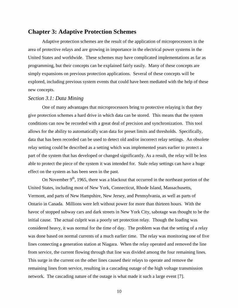
Chapter 3: Adaptive Protection Schemes

Adaptive protection schemes are the result of the application of microprocessors in the

area of protective relays and are growing in importance in the electrical power systems in the

United States and worldwide. These schemes may have complicated implementations as far as

programming, but their concepts can be explained fairly easily. Many of these concepts are

simply expansions on previous protection applications. Several of these concepts will be

explored, including previous system events that could have been mediated with the help of these

new concepts.

Section 3.1: Data Mining

One of many advantages that microprocessors bring to protective relaying is that they

give protection schemes a hard drive in which data can be stored. This means that the system

conditions can now be recorded with a great deal of precision and synchronization. This tool

allows for the ability to automatically scan data for preset limits and thresholds. Specifically,

data that has been recorded can be used to detect old and/or incorrect relay settings. An obsolete

relay setting could be described as a setting which was implemented years earlier to protect a

part of the system that has developed or changed significantly. As a result, the relay will be less

able to protect the piece of the system it was intended for. Stale relay settings can have a huge

effect on the system as has been seen in the past.

On November 9th

, 1965, there was a blackout that occurred in the northeast portion of the

United States, including most of New York, Connecticut, Rhode Island, Massachusetts,

Vermont, and parts of New Hampshire, New Jersey, and Pennsylvania, as well as parts of

Ontario in Canada. Millions were left without power for more than thirteen hours. With the

havoc of stopped subway cars and dark streets in New York City, sabotage was thought to be the

initial cause. The actual culprit was a poorly set protection relay. Though the loading was

considered heavy, it was normal for the time of day. The problem was that the setting of a relay

was done based on normal currents of a much earlier time. The relay was monitoring one of five

lines connecting a generation station at Niagara. When the relay operated and removed the line

from service, the current flowing through that line was divided among the four remaining lines.

This surge in the current on the other lines caused their relays to operate and remove the

remaining lines from service, resulting in a cascading outage of the high voltage transmission

network. The cascading nature of the outage is what made it such a large event [7].

11

Data mining and analysis could be implemented relatively easily in order to prevent

future events of this nature. Considering that power flows can change significantly on a seasonal

basis, these types of algorithms would probably need to be run on a monthly or biweekly basis.

The algorithm would simply be set up to detect percentage changes of average and peak records

for currents, voltages, angles, and any other variables measured by a particular relay since the

last time the relay was set by an engineer. Preset thresholds being breached would result in a

notification of the protection engineer responsible for the relay that needs attention. The main

concern is ensuring that the loadability of the relay is still acceptable. Loadability is simply the

amount of load that can be handled by a protection scheme before the relay operates due to

heavy loads rather than an actual fault condition. The loadability of the relays in the 1965

blackout in the northeast was satisfactory when they were set, but the growth of the load

exceeded the loadability of the relay and this caused the problem. The loadability will almost

always need to be increased, but there are occasions where it may be decreased in the case of a

shrinking load. Data mining and analysis can give protection engineers notice of potential

loadability issues far in advance of the development of an actual problem.

Section 3.2: Differential Protection

Differential protection schemes are set up simply to check for any difference between

two quantities at a given instance. Limitations on time synchronization made this

implementation only reasonable for equipment protection and difficult for other applications

until the recent advent of GPS signals. On the other hand, for signals collected from distant

points into a system, the burden of communication made the implementation of differential

protection difficult or unattainable. While this type of protection could be useful in detecting a

difference in current from one substation to the next, historically its application required the two

measurements to be taken very close to one another because of the constraints on

communication. So the scheme was limited generally to transformer and generator protection.

Before microprocessor-based systems and IEDs the nature of these two types of protection were

limited by several issues, specifically mismatches in current transducers.

Percentage differential protection of transformers finds the difference between two

current levels that should be close to equal. This is done by putting the output of two current

transducers in parallel with a relay that detects current flow. With the proper connection of

polarities of the CTs, if both the secondary currents are equal, no current will flow through the

12

relay. Issues with this include the previously stated mismatch due to CT limitations, as well as

CT error mismatches, transformer’s magnetizing currents, and tap changing elements which will

change the effective ratio of the transformer itself. These problems are alleviated by establishing

a restraint current. The restraint current is simply the average of the secondary currents. The

relay operates when the current that it sees exceeds a certain percentage of the restraint current.

The smaller the percentage required, the higher the sensitivity of the relay [2].

Additionally, magnetizing current can cause errors during energization and fault removal,

and its harmonic content can cause issues as well. The magnetizing inrush current is caused

when an unloaded transformer is brought online and needs to gain the flux necessary for steady

state operation to occur. This can also happen when a fault is cleared and the current changes

significantly. On top of magnetizing current, transformer over-excitation can also become a

problem. The saturation during these times can cause the differential relay to react

unnecessarily. Lastly, if there is a fault outside of the transformer it is possible that the CTs will

saturate at different current levels. If the difference between these saturation levels is large, the

differential relay will operate unnecessarily for a fault that is not within the transformer [2].

Computer based relays can offer solutions to all of these issues to significantly increase

the accuracy of operation for a percentage differential protection scheme. The main error caused

by mismatched ratios is quickly mediated by the fact that a computer can take the output from

any CT and scale it according to the turns ratio necessary for the secondary currents to match up.

In fact, the CTs do not even need to have secondary currents that are close to each other, but

simply take the current low enough for an analog to digital conversion to be given to the

computer. CTs can then be chosen based on their accuracy as well as their saturation limits in

order to prevent some of the other issues discussed.

The computer itself can be given inputs on different phenomena going on to prevent

unnecessary operation. For example, if the transformer is being brought online the computer can

be set to recognize and ignore the issues brought about by the inrush currents. In the case of a

transformer with tap changing occurring, the relay could be set up to allow for any inrush

currents expected as well as change the necessary ratios on the CTs. With certain

communication parameters, it could even be possible for a computer based differential relay to

recognize when faults outside of the transformer will affect operation of the relay. In the field of

communication, there are many opportunities to improve protection schemes.

13

Section 3.3: Communication

Modern protection engineers are at a great advantage because the growth of computers

now allows for digital communication between devices. Protection schemes in the past did have

ways of communicating between two distant points through technologies like pilot wire, power

line carriers, and microwave signals. The problem with these technologies is that the

contingencies affecting the lines they protect could jeopardize the communication systems

themselves. Microprocessor based relays can now simply access the internet or intranets in order

to communicate with other relays. These connections provide new sources of communication to

pass data between relays.

Older forms of communication are based on direct links. Pilot wire is simply a

communication wire hung on the same poles as the transmission lines themselves. Power line

carrier uses the power line conductor as the communication media. Microwave communication

involves transmitters and antennae transmitting data down the line wirelessly, but requires a

direct line of sight. Each of these methods has their own advantages and disadvantages with

regard to the types of schemes that they use. In power line carriers, blocking schemes are used,

where if there was a fault that was determined to be outside of the protected line, a blocking

signal was sent to the other side of the protected line in order to prevent unnecessary tripping. If

the line itself was compromised during the fault and the communication fails, the line should be

removed from service anyway, so the absence of the blocking signal would be ok. The issue

here is that it may be necessary for the other side to operate to isolate the fault in a backup

capacity. In communication forms that are separate from the power line itself, tripping schemes

are usually implemented. In tripping schemes, a signal is sent to the adjacent substation to take

the line out of service. If the communication fails, however, lines may fail to be removed when

they should be [2]. With communication via the internet and dedicated intranets, these schemes

could be altered and the communication links themselves can be monitored for operability.

Now data can be passed great distances between substations quickly and accurately with

more data points than before. Quickly is a relative term when it comes to the power system. On

the internet, latency and heavy traffic could slow down communication so schemes requiring

instantaneous communication would require a dedicated intranet. Using an intranet, snapshots

from adjacent substations can expand the abilities of differential protection beyond transformer

protection. Adjacent stations can monitor whether the current they are sending is the same as the

14

current being received at the other end. Using the internet, the accuracy of the data points being

collected could be validated through synchronized data collection. An accurate time tag will

allow for the coordination of data taken over a wide area. If the voltage between two stations is

significantly different, but all other factors like the angle between voltage and current, as well as

outgoing and incoming current indicated normal operation, it could be determined that the

voltage measurements are not being accurately recorded. This doesn’t necessarily require

immediate action, and could work even with heavy traffic on the network. These advancements

could significantly reduce unwanted actions in protective relaying.

15

Chapter 4: Transmission Level Adaptive Protection

As it has been explained before, adaptive protection schemes can be designed,

implemented and deployed into many different elements and systems of the power network. As

an example, this document will fully explore the benefits of adaptive protection as it is applied to

transmission line distance protection.

Section 4.1: Transmission Basics

A transmission line has four parameters that control the capacity and performance of

operation: resistance, inductance, conductance and capacitance. Material characteristics such as

resistivity, electric permittivity and magnetic permeability together with physical dimensions

such as radius of conductors, distance between conductors affect the four above listed

parameters. However, conductance between conductors and/or conductance between conductors

and ground may be considered negligible as it accounts for such a small portion of the

impedance characteristics. The other three parameters, resistance, inductance, and capacitance,

are the main focus when it comes to transmission line modeling.

One thing that complicates AC systems is the introduction of complex power. There are

capacitive and inductive elements associated with electricity. In a capacitor, the current going

into the element is dependent on the derivative of the voltage across the element. In an inductor,

the voltage is dependent on the derivative of the current going into the element. In a steady-state

DC system, these currents and voltages are constant, making the effect of capacitive and

inductive impedances negligible. The sinusoidal nature of AC systems, however, causes

inductive and capacitive impedances. While these elements do not actually consume any real

power, they affect something called reactive power, which in combination with the real power

consumed in a system is called complex power [5].

While there are simply elements called inductors and capacitors that can be plugged into

a circuit, the transmission lines that carry electricity to the customers have both a series

inductance and a shunt capacitance associated with them. In DC circuits, this would not be an

issue, but the sinusoidal nature of the voltages in AC systems causes these inductances and

capacitances to look like reactive impedance. Similar to the reactive power, it behaves like a

resistance in the AC domain; however it does not consume real power. These reactive

impedances can be found using mathematics [6].

16

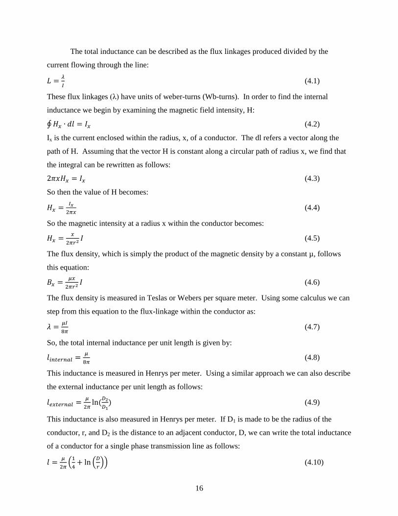
The total inductance can be described as the flux linkages produced divided by the

current flowing through the line:

(4.1)

These flux linkages (λ) have units of weber-turns (Wb-turns). In order to find the internal

inductance we begin by examining the magnetic field intensity, H:

∮ (4.2)

Ix is the current enclosed within the radius, x, of a conductor. The dl refers a vector along the

path of H. Assuming that the vector H is constant along a circular path of radius x, we find that

the integral can be rewritten as follows:

(4.3)

So then the value of H becomes:

(4.4)

So the magnetic intensity at a radius x within the conductor becomes:

(4.5)

The flux density, which is simply the product of the magnetic density by a constant µ, follows

this equation:

(4.6)

The flux density is measured in Teslas or Webers per square meter. Using some calculus we can

step from this equation to the flux-linkage within the conductor as:

(4.7)

So, the total internal inductance per unit length is given by:

(4.8)

This inductance is measured in Henrys per meter. Using a similar approach we can also describe

the external inductance per unit length as follows:

(4.9)

This inductance is also measured in Henrys per meter. If D1 is made to be the radius of the

conductor, r, and D2 is the distance to an adjacent conductor, D, we can write the total inductance

of a conductor for a single phase transmission line as follows:

(

(

)) (4.10)

17

The inductance for three phase systems is a bit more complicated depending on the spacing

between conductors, but there are several important points to notice from this equation. The two

main factors affecting the inductance are the distance between conductors and the radii of the

conductors. In higher voltage lines, the distance between conductors, D, must be larger for

insulation purposes, which will increase the inductance. If the conductors are larger in radius, r,

the inductance will decrease, and these effects will be limited as they are within the natural log

part of the argument in Eqn 4.10 [6].

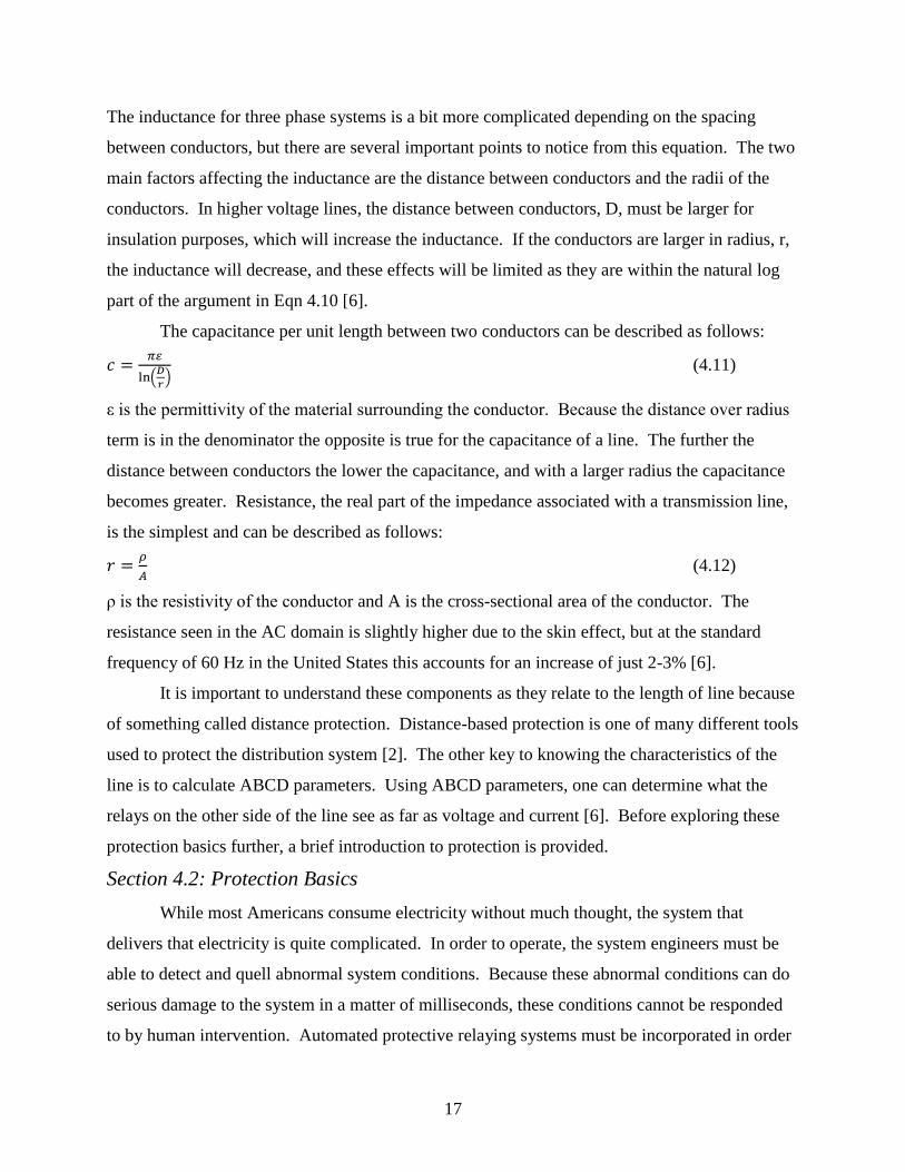
The capacitance per unit length between two conductors can be described as follows:

(

) (4.11)

ε is the permittivity of the material surrounding the conductor. Because the distance over radius

term is in the denominator the opposite is true for the capacitance of a line. The further the

distance between conductors the lower the capacitance, and with a larger radius the capacitance

becomes greater. Resistance, the real part of the impedance associated with a transmission line,

is the simplest and can be described as follows:

(4.12)

ρ is the resistivity of the conductor and A is the cross-sectional area of the conductor. The

resistance seen in the AC domain is slightly higher due to the skin effect, but at the standard

frequency of 60 Hz in the United States this accounts for an increase of just 2-3% [6].

It is important to understand these components as they relate to the length of line because

of something called distance protection. Distance-based protection is one of many different tools

used to protect the distribution system [2]. The other key to knowing the characteristics of the

line is to calculate ABCD parameters. Using ABCD parameters, one can determine what the

relays on the other side of the line see as far as voltage and current [6]. Before exploring these

protection basics further, a brief introduction to protection is provided.

Section 4.2: Protection Basics

While most Americans consume electricity without much thought, the system that

delivers that electricity is quite complicated. In order to operate, the system engineers must be

able to detect and quell abnormal system conditions. Because these abnormal conditions can do

serious damage to the system in a matter of milliseconds, these conditions cannot be responded

to by human intervention. Automated protective relaying systems must be incorporated in order

18

to prevent serious harm to the system. In order to ensure that abnormal conditions do not

adversely affect the system, the protective relaying put in place generally has a primary action

which is backed up by secondary actions. There are many forms of protective relaying that are

deployed based on the abnormal conditions expected [2].

While abnormal conditions can refer to any number of scenarios, most protection systems

are designed to clear a fault on the system. A fault occurs when current has a path straight to the

ground or from one conductor to another. When this path forms the impedance of the circuit

essentially becomes a combination of the path impedances of adjacent lines, the impedance of

transformer units and the intrinsic impedance of the generators. However, for strong systems

with multiple parallel paths and generators, this impedance may be low and the resulting fault

currents will have large magnitudes and possibly damaging effects [6]. When a permanent fault

exists, the portion of the system must be isolated. If the fault is in the middle of a transmission

line, that line must be disconnected at both ends at the substations that the line connects. This

disconnection is executed based on the type of protection being used [2].

Section 4.3: Development of Protection Schemes

The fuse is the simplest and oldest protection device used in electrical systems. What

makes it so simple is that its detection of the abnormal condition is also what causes the

interruption of the circuit. If the current exceeds a certain level, the fuse melts which breaks the

path for current to flow. While the simplicity of a fuse makes it very useful in specific situations,

the transmission system has become too complicated for fuses alone. The development of new

schemes allows for the remote re-closure of breakers, modification of relay settings, and others

that will be discussed. The next chronological step in the development of protection was the

introduction of electromechanical relays [2].

Electromechanical relays can operate on the same limits as fuses, but they offer a lot of

new options. In an electromechanical relay, the device that measures the levels operates by

signaling the circuit to interrupt, but they are two distinct functions. In the simplest case, a relay

will use the magnetic field produced by a level of current to physically move an object. The

movement of the object can open the circuit directly, like a circuit breaker in a home, or the

movement can close the contacts of a relay which allow for the disconnection of the circuit

elsewhere. This movement can have a single input, or several. This can become more complex

at the solid state and digital level [2].

19

Solid state relays bridge the gap between the original electromechanical relays and the

computer-based relaying in use today. Solid state relays operated using integrated circuits, rather

than physically moving parts. Though not as robust as their predecessors, they could be adjusted

to maintain much tighter tolerances, and were more consistent in operation. The logic and inputs

available to a solid state relay were what allowed the simpler implementation of the Mho relay,

or distance relay. Before this development, the centers of the zones of protection were moved

away from the origin of the R-X plane using complex voltage divider circuits. This was

extremely complex to implement. Within solid state relays, however, the Mho relay was much

simpler to implement. Even more advanced than solid state technology, however, is the

development of computer-based relays [2].

Computer based relays open many opportunities for protection engineers. Not only do

computers allow for in depth analysis for relay action, they also allow for communication with

other parts of the system for added information. Initially, however, computer based relays were

designed to mimic their predecessors. A lot of the functionality built into computer based relays

on the market today is based on protection schemes that could be implemented with simpler

components. The communication aspect of computers allows system operators to monitor the

state of the system and allows them to be proactive in keeping the system working smoothly [2].

While there are some very advanced techniques that can be employed, they will be discussed in

context with the schemes of protection being proposed.

Before explaining the advanced techniques, some background on the operation of

computer based relays may be necessary. The high voltage transmission operates on the order of

hundreds of kilovolts and on the order of kiloamps for voltage and current respectively. The

issue is that computers generally operate on the order of volts and milliamps. So in order to

make measurements on the high voltage system, the measurements are made on voltages and

currents that are stepped down using transformers. The current transformers work on the same

principle as the transformers that are used to step voltages up and down for transmission

purposes. They are coupled magnetically to the transmission line and step down the current from

the primary current of kiloamps to a standard value on the secondary. The primary is simply the

value of the current on the transmission line and the secondary is the level that is measured. The

standard value for secondary currents in the United States is 5 amps. The computer can take the

measured value and multiply it by the ratio of primary to secondary current in order to find the

20

value of the primary. This ratio is often called the turns ratio in this type of transformer because

the ratio depends on the number of coils, or ‘turns,’ there are in the transformer on the primary

and secondary side [2].

Voltage transformers can operate in the same way, but there is another style of

transformer that is also used which is directly connected to the line. A capacitor coupled voltage

transformer, or CCVT, is a set of capacitors connected together in series between the line being

measured and ground. The voltage across each of these capacitors can be calculated using the

principle of voltage division. As a result, only a fraction of the voltage may be delivered to the

instrumentation of the line. The proportion factor of the line voltage to the output of the CCVT

is known and given by a ratio of the capacitances used in this implementation. Capacitors are

used because they do not actually consume real power as discussed earlier. The standard voltage

on the secondary is 120 volts if measuring between two lines, or 69.3 volts if measuring between

a line and ground. This may be done in multiple steps of a CCVT stepping the voltage down to a

few kilovolts, then a traditional voltage transformer to step the voltage down to the standard

secondary values [2].

The next step is to convert the reduced voltages and currents into digital values. This is

done using an analog to digital converter. The converter takes the value of the secondary and

freezes it using a sample and hold circuit, this allows for simultaneous samples. The value is

held to give the converter ample time to convert the analog value into a digital value. The digital

value is then given to the computer to be handled like any other data. Also, with the aid of a

common time signal which can be received from the Global Positioning System satellites, data

that is stored in many locations can be synchronized to study events that happen on the network.

This is very important for post-mortem analysis of catastrophic events on the system. The

analysis of these events can be used to develop new forms of protection, like the one that will be

developed later in this chapter [2].

A computer relay can also check on the performance of other adjacent relays as well. A

computer relay can use ABCD parameters to determine what the relay at the other end of the line

should be seeing. The ABCD parameter concept uses the voltages and currents measured at one

substation to determine what the measurements should be at the other end of the line. This is

done by using the pre-calculated parameters that feed into the following equations:

(4.13)

21

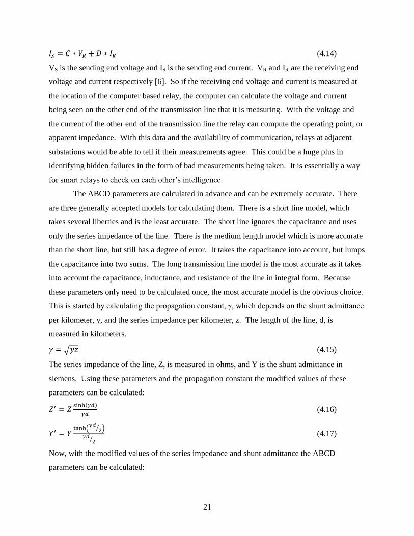
(4.14)

VS is the sending end voltage and IS is the sending end current. VR and IR are the receiving end

voltage and current respectively [6]. So if the receiving end voltage and current is measured at

the location of the computer based relay, the computer can calculate the voltage and current

being seen on the other end of the transmission line that it is measuring. With the voltage and

the current of the other end of the transmission line the relay can compute the operating point, or

apparent impedance. With this data and the availability of communication, relays at adjacent

substations would be able to tell if their measurements agree. This could be a huge plus in

identifying hidden failures in the form of bad measurements being taken. It is essentially a way

for smart relays to check on each other’s intelligence.

The ABCD parameters are calculated in advance and can be extremely accurate. There

are three generally accepted models for calculating them. There is a short line model, which

takes several liberties and is the least accurate. The short line ignores the capacitance and uses

only the series impedance of the line. There is the medium length model which is more accurate

than the short line, but still has a degree of error. It takes the capacitance into account, but lumps

the capacitance into two sums. The long transmission line model is the most accurate as it takes

into account the capacitance, inductance, and resistance of the line in integral form. Because

these parameters only need to be calculated once, the most accurate model is the obvious choice.

This is started by calculating the propagation constant, γ, which depends on the shunt admittance

per kilometer, y, and the series impedance per kilometer, z. The length of the line, d, is

measured in kilometers.

√ (4.15)

The series impedance of the line, Z, is measured in ohms, and Y is the shunt admittance in

siemens. Using these parameters and the propagation constant the modified values of these

parameters can be calculated:

(4.16)

(

⁄ )

⁄

(4.17)

Now, with the modified values of the series impedance and shunt admittance the ABCD

parameters can be calculated:

22

(4.18)

(4.19)

(

) (4.20)

(4.21)

These four values are each complex numbers, meaning they have a magnitude and angle

associated with them. The series impedance and shunt admittance can be calculated as noted

earlier, using the size and spacing of the conductors [6].

Section 4.4: Distance Protection

Fuses and other similar devices are simple in that they react based solely on one input. If

the current gets to a certain level the circuit is shut off. In distance protection, a relay actually

determines whether it will react based on multiple parameters. Specifically, it reacts based on

the voltage and current measured going through a circuit, as well as the angle between the

voltage and current. With these three parameters, the relay determines the apparent impedance

of the circuit as seen from its own terminals. If there is a fault on the line, this apparent

impedance will work out to be the impedance of the line between the relay and the fault plus the

fault impedance itself. This impedance is

based on the previously discussed

characteristics of a transmission line. It is

generally plotted in the R-X plane, where the

R refers to the real part of the impedance

seen, and the X refers to the reactive

component of that impedance. The

protective relay has preset limits for which it

will react [2].

The R-X plane can be best described visually as seen in Figure 1. The reactive

impedance is on the vertical axis, and the real impedance is on the horizontal axis. Both of these

quantities are measured in Ohms generally, but they may be given in per-unit. Using the

formulas described earlier, one can find the impedance of a transmission line in order to plot it in

the R-X plane. The black line shows a typical transmission line as far as the ratio between real

and reactive impedance. Also shown are some of the typical characteristics employed in a

Figure 1

23

distance-based protective relay. Figure 1 shows two sets of limits for the relay. If the black line

was a transmission line between two points, the green circle would represent what is called the

2first zone of protection. The diameter of the green circle is set to encompass between 85% and

90% of the line that it is intended to protect, and is set on the side of the transmission line where

the relay is taking its measurements. If the apparent impedance seen by the relay enters this

zone, the relay immediately cuts off power to the transmission line. The blue zone is called the

second zone of protection. It typically encompasses about 120% of the line that it is intended to

protect. Because zone two may also see a fault that is on an adjacent line a small delay is built in

before it would cut power to the transmission line as to allow the zone one of that adjacent line to

react if the fault is on that line. In addition to the

first two zones, there is usually a third zone of

protection that is also employed whose diameter

is equal to 150% of the next adjacent line in

addition to 100% of the line the relay is primarily

looking at. With this third zone of protection, the

adjacent line has a backup in case the first two

zones fail to react to a fault, or the device that

turns off the power to the transmission line fails

to operate, known as breaker failure [2].

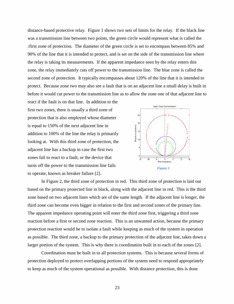
In Figure 2, the third zone of protection in red. This third zone of protection is laid out

based on the primary protected line in black, along with the adjacent line in red. This is the third

zone based on two adjacent lines which are of the same length. If the adjacent line is longer, the

third zone can become even bigger in relation to the first and second zones of the primary line.

The apparent impedance operating point will enter the third zone first, triggering a third zone

reaction before a first or second zone reaction. This is an unwanted action, because the primary

protection reaction would be to isolate a fault while keeping as much of the system in operation

as possible. The third zone, a backup to the primary protection of the adjacent line, takes down a

larger portion of the system. This is why there is coordination built in to each of the zones [2].

Coordination must be built in to all protection systems. This is because several forms of

protection deployed to protect overlapping portions of the system need to respond appropriately

to keep as much of the system operational as possible. With distance protection, this is done

Figure 2

24

with a time delay. This is more specifically dependent upon what is used to interrupt the circuit.

If the first zone of protection is breached, it should react immediately. It takes about a third of a

second for the first zone to see the fault and turn off the circuit to isolate the fault. Built into the

second zone of protection is roughly a 300 millisecond delay before it will attempt to isolate a

fault that it sees. Then, the third zone of protection has a delay of about one full second. These

delays prevent unnecessary operation of secondary protection.

Another important concept to understand in the three zone distance protection scheme is

loadability. The magnitude of the apparent impedance is found by dividing the voltage by the

current. So as the load increases the current increases as well, and while the voltage remains

relatively constant, the apparent impedance shrinks. The limit at which loading could cause the

apparent impedance to encroach on the third zone of protection is called the loadability limit.

The following two equations describe the loadability of a basic impedance relay and a mho relay,

like the ones described in the figures, respectively:

(4.22)

(4.23)

With the value of Z in the denominator, the loadability will increase if the protected zones are

smaller, as the voltage, E, is generally held constant [2]. This loadability can be altered by

changing the shape of the zones of protection, but each shape has tradeoffs. The closer the zones

are trimmed toward the transmission line in the R-X plane the greater the increase in loadability,

but this comes at the price of vulnerability to high impedance faults. If the fault is not directly to

ground, the added fault impedance may cause the operating point to fall outside the zones of

protection.

Now that the basics of protections schemes have been reviewed, it is possible to delve

further into a new concept in adaptive relaying applications. This new concept has been

developed in direct response to the loadability problems associated with the third zone of

protection. To fully grasp the problems that loadability can cause we will take a look at the 2003

blackout of the northeast United States and Canada. While there have been many power

disruptions, this one was easily the largest to ever strike the United States. With the help of

adaptive protection schemes, hopefully the 2003 blackout will remain the largest blackout to

strike the United States.

25

Section 4.5: 2003 Northeast Blackout

On August 14th

, 2003 the northeast United States sustained its largest cascading outage.

The report regarding the blackout, released in April of 2004, details a very complex set of events

that led to the blackout. It started in Ohio due to poor load forecasting and system maintenance.

Summer heat and poor tree-trimming practices led to the loss of several lines because they had a

path to ground through overgrown trees near transmission lines. This, coupled with a computer

failure for operators, led to alarm functions being disabled. These events put the high voltage

transmission system into a highly stressed state. This was compounded by reactive power

resources being out of service for maintenance. This system stress in Ohio led to a cascading

blackout that blacked out an estimated 50 million customers in Ohio, Michigan, Pennsylvania,

New York, Vermont, Massachusetts, Connecticut, and New Jersey in the United States, as well

as Ontario in Canada. It took up to four days for some customers to have their power restored in

the United States, and some parts of Canada were forced to deal with rolling blackouts for more

than a week. The blackout cost upwards of four billion dollars, and while certain aspects of it

were unavoidable, the cascading across the northeast could have been prevented[3].

The fact that a blackout occurred that day was

inevitable, but the size of the outage could have been

significantly reduced. Problems started with the

Midwest Independent Transmission System Operator,

MISO, feeding inaccurate data to their state estimator.

The state estimator is what the operators use to

determine the output needed from individual generating

plants, the loss of which is manageable. This was

followed by the loss of a key generating station that belonged to First Energy (FE). FE then lost

the system which controlled their alarms. This was mainly affecting the city of Cleveland, a

large load center in Ohio. The real and reactive power supply necessary for a stable voltage

profile was put in jeopardy by the loss of the generating station, as there were already other

resources out for maintenance. FE then began losing high voltage transmission lines due to trees

making contact with lines, an event that is more likely to occur due to higher currents generating

more heat leading to sagging lines. The lack of alarms, however, meant that neighboring

systems were noticing the problems before FE. The stress on the system in the Cleveland area

Figure 3

26

may have been isolated to the Cleveland area had the line between the Sammis and Star

substations not been lost. The Sammis-Star line was, however, lost due to an encroachment on

Zone 3. This line is labeled as 5A in Figure 3 which was taken from the final report of the 2003

Blackout. The blackout of the Cleveland area was pretty much inevitable, but it could have been

isolated there had the third zone of protection not reacted inappropriately. Also, had the

Sammis-Star line remained online the neighboring systems of FE may have been able to take

action by shedding loads in order to maintain the system[3].

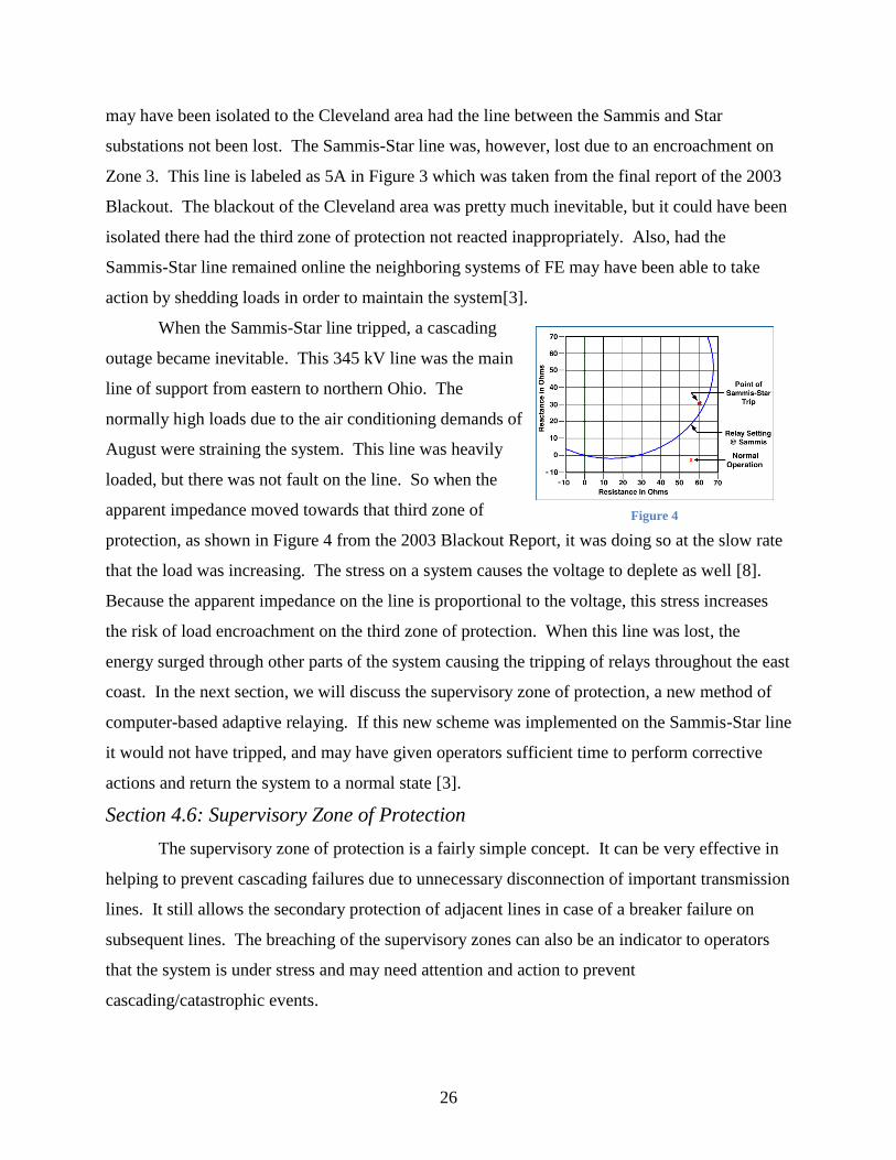
When the Sammis-Star line tripped, a cascading

outage became inevitable. This 345 kV line was the main

line of support from eastern to northern Ohio. The

normally high loads due to the air conditioning demands of

August were straining the system. This line was heavily

loaded, but there was not fault on the line. So when the

apparent impedance moved towards that third zone of

protection, as shown in Figure 4 from the 2003 Blackout Report, it was doing so at the slow rate

that the load was increasing. The stress on a system causes the voltage to deplete as well [8].

Because the apparent impedance on the line is proportional to the voltage, this stress increases

the risk of load encroachment on the third zone of protection. When this line was lost, the

energy surged through other parts of the system causing the tripping of relays throughout the east

coast. In the next section, we will discuss the supervisory zone of protection, a new method of

computer-based adaptive relaying. If this new scheme was implemented on the Sammis-Star line

it would not have tripped, and may have given operators sufficient time to perform corrective

actions and return the system to a normal state [3].

Section 4.6: Supervisory Zone of Protection

The supervisory zone of protection is a fairly simple concept. It can be very effective in

helping to prevent cascading failures due to unnecessary disconnection of important transmission

lines. It still allows the secondary protection of adjacent lines in case of a breaker failure on

subsequent lines. The breaching of the supervisory zones can also be an indicator to operators

that the system is under stress and may need attention and action to prevent

cascading/catastrophic events.

Figure 4

27

The supervisory zone of protection is intended to give operators the ability to have both

security and dependability when each is more appropriate. This is a growing trend in computer

based relaying, where protection engineers can design algorithms that will behave dependably

when the system is normal and an unnecessary loss of a line is not a big risk. These same

algorithms can sense a stressed system state and force the protection schemes to be more secure,

so that lines aren’t lost unnecessarily. This is the concept behind the supervisory zone of

protection, and as it will be explained later, doesn’t require a lot of input to detect the stress and

can be easily implemented using computer-based relays available in the market today.

The supervisory zone is essentially a fourth

zone that the relay monitors. Unlike the three

standard zones of protection, the supervisory zone

does not have a tangent at the origin of the R-X

plane. The supervisory zone is concentric with the

third zone of protection and, for the purposes of

this implementation, is between 20% and 30%

larger than the third zone. This can be seen in

Figure 5. The largest circle in the diagram is the

supervisory zone.

There are two scenarios for the operation of the third zone of protection. One is that there

is a fault on the system, during which the operating point almost instantaneously moves from a

far distance away from the third zone border, the equivalent R-X value of a load, to the inside of

zone three, the R-X value of a fault. The second scenario corresponds to a monotonically

increasing load and causes the operating point to slowly creep towards and encroach on the third

zone. The problem is that the relays cannot distinguish between the fault which needs to be

removed from the system, and the overload encroachment which, if disconnected, may

contribute to a cascading outage.

The supervisory zone of protection distinguishes between these two scenarios by

determining how quickly the operating point is moving. When the operating point breaches the

supervisory zone a timer is started. If the timer reaches the predetermined set point before

breaching the third zone, the relay can block the third zone from operating. If the third zone is

breached before the set point is reached it is allowed to operate normally. So if the system is

Figure 5

28

heavily loaded, the slow moving operating point will cause the timer to reach the set point and

disable the third zone to prevent an unnecessary trip. If the system is faulted and the third zone

needs to operate as a backup it is allowed to do so. This is what allows security or dependability

depending upon system stress. The set point of the timer needs only to be large enough that it

won’t incorrectly prevent a third zone action during a fault, so a sufficient timer would be

discovered by running simulations to determine the absolute slowest possible crossing of both

boundaries under a fault condition. Once the period of the maximum fault condition boundary is

determined, the relay can be set to inspect the operating point at a frequency which has a

matching period. This is because the expected maximum fault condition period is on the order of

milliseconds or cycles while the expected crossing during a load encroachment is on the order of

seconds or even minutes. This means the relay does not need to constantly calculate the

supervisory zone condition which reduces the computational stress on the relay. An important

thing to realize is that this timer should only be running if Zone 3 is not encroached. If Zone 3 is

encroached, the Zone 3 timer will need to run for coordination.

The supervisory zone of protection is not the first scheme to try to prevent load

encroachment. Changing the shape of the zones of protection has also been done to try to

increase loadability. As discussed before, this could stop a relay action from isolating a high

impedance fault. Therefore, even with relays that have modified protection zones, the shapes are

fixed and cannot adapt to system changes. On the other hand, off-line system simulations and

studies can be provided with enough information to adequately set the timers that separate faults

from transient loads. The classification between fast-moving fault impedance and slow-moving

load encroachment could help eliminate false tripping and mitigate some of the factors that

contribute to large scale system blackouts.

29

Chapter 5: Implementation of the Supervisory Zone of Protection

The supervisory zone of protection can be implemented on any computer based relay that

can measure the voltage and current and the phase angle between them. From that point, the

programming aspect, which most computer based relays allow, is quite simple. It only depends

on how the current and voltage are stored and made available to the programmer. They can be

stored either in polar or rectangular form. Polar form being the magnitude and angle, and

rectangular being the real and imaginary components. To go between the two, the following

formulae can be used, where M is the magnitude and θ is the angle in polar form, and Re and Im

are the Real and Imaginary components in rectangular form:

(5.1)

(5.2)

√ (5.3)

(

) (5.4)

The equivalent apparent complex impedance, as seen from the terminals of the protective relay,

can be computed by the ratio of voltage and current. For a balanced loading condition, all phases

will report the same impedance. This information may also be useful in discriminating between

a fault and a load because most faults are unbalanced and would show a different impedance on

each phase. This ratio, performed with quantities in polar form can provide us with the two

elements of the impedance, magnitude and angle:

(5.5)

(5.6)

This calculated equivalent impedance together with the corresponding boundaries of the

protected zones of a Mho or Impedance relay can help us determine the state of the system;

meaning is it in normal or abnormal operation. It should be noted that normal operation is

considered as an operating point outside the area of operation of the relay while abnormal would

correspond to points inside one of the operating contours of the same relay.

As it was indicated earlier, each of the zones of protection of a relay is established based upon

the impedance of the line that is protecting for zones 1 and 2. The third zone (zone 3) is

determined using the impedance of the protected line and the subsequent longer line. Equation

30

5.7 below is used to determine if an operating point corresponds to a point within the areas of

operation. So to calculate the distance we use the following:

√ (5.7)

Obviously, the impedance needs to be converted from polar as calculated to rectangular as

shown earlier. In order to reduce computational intensity, it is simpler not to take the square root

as shown and compare the result to the square of the radius of each of the zones. If the

supervisory zone has been encroached, but the operating point is still outside of the third zone of

protection a timer should start running. If the timer reaches the simulation-determined maximum

period for a fault before the third zone of protection is encroached, the third zone of protection

should be disabled. If the operating point leaves the supervisory zone, the third zone of

protection should be re-enabled. It is important to note that normal distance protection generally

employs six different relay settings to include all balanced and unbalanced fault conditions. The

purpose of the Supervisory Zone, however, is to prevent a load encroachment which generally

only occurs as a balanced load. Though the Supervisory Zone would block Zone 3 operation of

all six different relays, it would only need to calculate the apparent impedance as seen by the

relays responsible for a three phase fault.

Section 5.1: Hardware Implementation

In order to prove the

concept, the programming

was done on a relay from

Schweitzer Engineering

Laboratories. The SEL-421 is

a high speed line protection,

automation, and control relay.

Using the AcSELerator

QuickSet software available

from Schweitzer, there are

multiple options which can be

used to program the relay.

For simplicity, there is a

feature that allows programming to be done as a block diagram which can then be translated into

Figure 6

31

the coding necessary within the

relay. This can be seen in Figure

6. As an example, VBLPMM is

the magnitude of the voltage

phasor measured on phase B.

VBLPMA is the corresponding

angle of this voltage phasor.

IBSPMM and IBSPMA are the

magnitude and angle of the current

phasor measured on phase B.

These are used to calculate

ZBCEN, which is the square of the

distance between the center of the

zone three protection and the

operating impedance. This is then

compared to a preset value.

BZONES is true when the

operating point is within the supervisory zone, and BZONE3D is true when the supervisory zone

has been encroached for more than a full second. Thus, the trip logic simply needs to be set to

only trip for zone three if the BZONE3D bit is false.

The advantage of this

style of programming is that it

is simple for novice

programmers to complete. The

AcSELerator software

translates this block diagram

into the code necessary for the

relay to operate. Without the

AcSELerator software, the

programmer would need to use

the hyper terminal to communicate with the relay and do the necessary programming. Even with

Figure 8

Figure 7

32

this complication, Figure 8 demonstrates that the translated code is still simple. There are less

than twenty lines of code to enter for each phase being protected. The relay was loaded with

these new protection settings for testing.

Schweitzer has also produced a testing

platform that can be used to test their relaying

equipment. The Adaptive Multichannel

Source, SEL-AMS, has voltage and current

outputs that can be used as inputs to relays.

The SEL-AMS simulates the secondary

voltages and currents that would be measured

by the relay after the step down transformers.

The SEL-AMS is operated using SEL-5401

Test System Software. The software allows

for the programming of different system

conditions to evaluate relay performance under

different test scenarios. In order to test the

supervisory zone of protection, five states

were to be simulated by the AMS, each lasting

for five seconds. The first state is set to

simulate normal operating conditions and has

an operating point outside of the supervisory

zone of protection. This can be seen in Figure

11. The second state simulates a stressed

system condition where the operating point is

within the supervisory zone of protection but

outside of the third zone of protection and can

be seen in Figure 10. The third state simulates

the crossing of the third zone of protection

during a load encroachment scenario and can

be seen in Figure 9. The fourth state simulates

Figure 11

Figure 10

Figure 9

33

a return to normal operating conditions as seen in Figure 11. The fifth state simulates a fault for

which the third zone of protection would need to operate and can be seen in Figure 12.

During each of these trials, the ZONES

and ZONE3D bits had their states displayed by

lights on the front of the SEL-421. The relay

tripping function was also displayed by a light

on the front of the relay. During the first system

state, none of the lights were lit indicating that

everything was normal. During the second

system state, the ZONES bit came on

immediately as the operating point entered the

supervisory zone, and after one second, the

timer associated with the load encroachment algorithm was completed, and the ZONE3D bit

came on. This was an indication that the supervisory zone of protection was disabling the third

zone of protection. During the third system state both of these lights remained on, and the

indicator for the encroachment of the third zone of protection came on, but the relay did not trip.

During the fourth system state, all of these lights were cleared indicating normal operation.

During the fifth system state the ZONES light came on along with the third zone’s indicator and

the relay tripped after the appropriate zone three delay before the ZONE3D could turn on and

disable the third zone of protection. This testing of the relay shows operation precisely as

designed and implemented.

There were some issues that arose during the testing before obtaining the desired result.

The block diagram programming required that the output of certain operations had to be stored to

a register and then called from that register for the next operation. While this was difficult to

troubleshoot, it did allow for a cleaner looking block diagram in the end. The reasoning for the

extra steps is unclear, but it is likely that the processor can only handle so many mathematical

operations in a single line of code. The stored data points can also be useful because they could

be compared to several different thresholds if desired.

This implementation of the supervisory zone was both simple and successful. This zone

provides an easy way for a computer based relay to distinguish between a fast moving fault and a

slow moving load encroachment. It does this by tracking the speed of the apparent impedance as

Figure 12

34

it crosses two different thresholds. The next logical step for future work would be to quantify the

actual rate of change of apparent impedance, and not just the breaching of thresholds in

succession.

35

Chapter 6: Future Work and Conclusions

The basic concept behind the supervisory zone of protection is to determine whether the

apparent impedance is moving quickly enough to be considered a fault. The advantage of the

supervisory zone is its simplicity. It does not require significant amounts of computation and

will not slow down a relay, but it does provide more information about the realm of the apparent

impedance and the rate at which it is moving. The supervisory zone detects the breach of certain

boundary limits, but it may be even more beneficial to measure the actual rate of change of an

operating point.

Section 6.1: R-R Dot

This concept was first developed by the Bonneville Power Administration in the early

1980s. In the fall of 1982, it was deployed to control the tripping of the 500 kV AC Pacific

Intertie. The initial application was an out-of-step protection scheme designed to react better to

unstable power swings. During unstable swings where the line should be taken out of service, it

is better for the system as a whole if the line is taken out of service before the swing reaches its

minimum voltage. This prevents severe voltage dips and uncontrolled loss of loads [9]. These

dips in voltage can cause shrinking impedance in distance protection schemes.

The disadvantage of tripping prior to this minimum is that unnecessary tripping is

possible, for example when the swing is recoverable. The R-R Dot scheme was developed to

distinguish between stable and unstable swings. This allows for earlier action during unstable

swings and better non-action during stable events. The reason for change from original out-of-

step schemes was that in the 15 years prior to this schemes implementation there had been a

separation or action by the scheme roughly once a year. None of these cases actually

corresponded to a severe fault for which the scheme was intended to react. The main reason for

operation of the older scheme was that stressed operating conditions caused the relay to react

inappropriately [9]. Though these separations may not have had the same effects as the 2003

blackout, the circumstances were very similar - a relay reacted inappropriately during a stressed

state and removed lines that should not have been removed from service.

Prior to this development, schemes had to base their settings on the worst case which has

several inherent problems. This meant that the intertie had poor transient stability performance,

in that it would disconnect when loss of synchronism would not be the case. Tripping at these

settings could mean that roughly half of the deceleration energy available by the equal area

36

criterion would not be available [9]. Therefore, the new scheme was developed in order to

improve performance.

The new R-R Dot scheme operated based on the real part of the impedance, the

resistance, rather than the complex impedance, but it started with the following logic in which

complex impedance was taken into account:

⁄ (6.1)

In this setup, U1 was the control output that would trip the circuit if it reached zero. Z was the

apparent impedance being measured; its derivative or rate of change is seen in the second term

on the right side of the equation. Z1 and T1 were both parameter settings to be adjusted for

desired performance [9]. If the impedance was decreasing very rapidly the derivative term

would be a large negative value, which would cause the relay to react even if the impedance term

was not crossing its threshold. A combination of the impedance and its derivative dictated when

the relay would trip.

For various reasons this concept was limited to the real resistance and its derivative. This

would allow for the relay to react regardless of the location of the swing relative to where the

measurements were taken. So the R-R Dot system was deployed on the 500 kV AC Pacific

Intertie with settings derived from intense simulation [9]. The scheme was enacted at the Malin

substation and was monitored for 18 months before it would actually control any tripping action.

Its primary use was for controlled separation, but added features included generator tripping,

series capacitor switching, dynamic braking, as well as shunt reactor and capacitor switching.

The conclusion was that the relay did perform better with the new R-R Dot scheme when it came

to distinguishing between stable and unstable swings [10].

Section 6.2: Conclusions

The supervisory zone of protection is a simple way to help a relay distinguish between a

fault condition and a load encroachment. It does this by determining how quickly the apparent

impedance seen by a relay is moving. By establishing the supervisory zone the relay can better

react to stressed system state abnormalities, which has been shown to be the culprit in the large

blackouts that have been seen in the past. The stressed system conditions that have led to these

problems in the past have proven to be more common, and will continue to become more

common as power system engineers are forced to do more with less. It is my belief that when

37

this concept is applied correctly it will not receive much notoriety; blackouts that are prevented

are much less notable than the blackouts that are not.

Furthermore, future endeavors of rate of change of impedance being a parameter within

protection schemes could lead to even better stability in the power system. With the rate of

change of impedance it could be possible for a relay to determine if a fault condition outside its

realm of protection was responded to correctly. With these innovations made possible by the

new tools given to protection engineers, prevention of blackouts and improvement of system

stability even under heavy stress is on the way.

38

References

1. Sulzberger, C.L., Triumph of AC - from Pearl Street to Niagara. Power and Energy

Magazine, IEEE, 2003. 1(3): p. 64-67.

2. Horowitz, S.H. and A.G. Phadke, Power System Relaying (3rd Edition), John Wiley &

Sons.

3. U.S.-Canada Power System Outage Task Force., Final report on the August 14, 2003

blackout in the United States and Canada : causes and recommendations2004, Ottawa:

Natural Resources Canada. vi, 228 p.

4. Triumph of AC. 2. The battle of the currents. Power and Energy Magazine, IEEE, 2003.

1(4): p. 70-73.

5. Grainger, J.J. and W.D. Stevenson, Power system analysis1994, New York: McGraw-

Hill.

6. Chapman, S.J., Electric machinery and power system fundamentals2002, Boston:

McGraw-Hill.

7. Vassell, G.S., Northeast Blackout of 1965. Power Engineering Review, IEEE, 1991.

11(1): p. 4.

8. Taylor, C.W., N.J. Balu, and D. Maratukulam, Power system voltage stability. The EPRI

power system engineering series1994, New York: McGraw-Hill. xiii, 273 p.

9. Taylor, C.W., et al., A New Out-of-Step Relay with Rate of Change of Apparent

Resistance Augmentation. Power Apparatus and Systems, IEEE Transactions on, 1983.

PAS-102(3): p. 631-639.

10. Haner, J.M., T.D. Laughlin, and C.W. Taylor, Experience with the R-RDOT out-of-Step

Relay. Power Delivery, IEEE Transactions on, 1986. 1(2): p. 35-39.

39

Appendix A

Figure 1: A demonstration of distance based protection relay parameters including the primary

and secondary zones, but not the third zone

Figure 2: A demonstration of distance based protection relay parameters including all three basic

protection zones

Figure 3: A map of the high voltage transmission system in the Ohio area, taken from the 2003

Blackout Report

Figure 4: A demonstration of the third zone of protection relay parameters, taken from the 2003

Blackout Report

Figure 5: A demonstration of the supervisory zone of protection as it relates to the first three

zones of protection

Figure 6: A screenshot of the encoding done in function block diagram form on the SEL-421

Figure 7: A basic flow chart of how the relay should react for the supervisory zone

Figure 8: A screenshot of the function block diagram translated into structured text in the SEL-

421

Figure 9: A demonstration of the operating point of an unstressed system used during testing

Figure 10: A demonstration of the operating point of a stressed system used during testing

Figure 11: A demonstration of the operating point of a load encroachment on a stressed system

used during testing

Figure 12: A demonstration of the operating point of a fault condition used during testing