Clemson UniversityTigerPrints

All Dissertations Dissertations

8-2016

The Adaptable Growth of Seashells: Informing theDesign of the Built Environment throughQuantitative BiomimicryDiana Ann ChenClemson University

Follow this and additional works at: https://tigerprints.clemson.edu/all_dissertations

This Dissertation is brought to you for free and open access by the Dissertations at TigerPrints. It has been accepted for inclusion in All Dissertations byan authorized administrator of TigerPrints. For more information, please contact kokeefe@clemson.edu.

Recommended CitationChen, Diana Ann, "The Adaptable Growth of Seashells: Informing the Design of the Built Environment through QuantitativeBiomimicry" (2016). All Dissertations. 1740.https://tigerprints.clemson.edu/all_dissertations/1740

THE ADAPTABLE GROWTH OF SEASHELLS: INFORMING THE DESIGN OF THE BUILT ENVIRONMENT THROUGH QUANTITATIVE BIOMIMICRY

A Dissertation Presented to

the Graduate School of Clemson University

In Partial Fulfillment of the Requirements for the Degree

Doctor of Philosophy Civil Engineering

by Diana Ann Chen

August 2016

Accepted by: Dr. Brandon Ross, Committee Co-Chair Dr. Leidy Klotz, Committee Co-Chair

Dr. Qiushi Chen Dr. Michael Carlos Barrios Kleiss

ii

ABSTRACT

Our current design philosophy in the creation and planning of our country’s

infrastructure exudes an attitude of nonchalance that is incongruous with the significant

impact the built infrastructure has on the natural environment. We are living through an era

of obsolescence, in which structures are demolished thoughtlessly as they outgrow their

ability to meet human demands. Obsolescence can be viewed as a “hazard” in the sense

that this phenomenon is leaving swaths of buildings in unusable and undesirable

conditions, lessening the quality of host locales, and polluting the environment with

demolitions and the need for more construction resources. Designing our buildings to be

adaptable to changing needs, rather than sufficient for predicted loads and functions, may

help mitigate the amount of unnecessary demolitions. However, designing adaptably is not

something we know how to do well; luckily, Nature has billions of years of experience that

we can turn to.

Biomimicry is a design approach that emulates Nature’s time-tested patterns and

strategies for sustainable solutions to human challenges. While biomimicry has been used

in many fields, applications in the built environment at the structures scale are scarce.

Moreover, the examples that we do see are largely concerning thermal regulation. Even

more troubling is how the popularization of biomimicry has led to frequent and misleading

claims that qualitative, conceptual inspiration is inherently sustainable, given mere

references of Nature.

This project pairs infra/structural problems with natural solutions to bring these

issues to attention in the civil engineering discipline. The spiraled shell of the Turritella

iii

terebra, a marine snail, is studied in this research to provide engineers with an example of

how to use biomimicry in a comprehensive way. The spiraled gastropod shell demonstrates

a simple form of adaptable growth, in which it is able to change its form through time to

meet increases in its own performance demands. This project discusses how the snail’s

environmental conditions influence its evolutionary traits through one of Nature’s

principles (form follows function). The shell is mathematically characterized and

structurally modeled to identify the functional roots responsible for its interesting resulting

form. By pinpointing the emergent properties leading to adaptable growth, we create an

opportunity to extract fundamental lessons of adaptability for application to the built

environment.

Shell samples of the T. terebra are experimentally tested with a structural

engineering lens, and a finite element (FE) model of the shell is validated with these results.

The FE model is then used to study parametric effects of ecological constraints—such as

drag on the shell, fracture due to predators, and living space—to identify how adjustments

to Nature’s design compare to reality. Many interesting findings about shell growth are

discussed; however, comparisons to human structures are generalized into three main

notions. The shell optimizes living convenience as it ages; the shell increases its external

load capacity with age/length; and the data suggests that the snail undergoes a change in

motivation for survival, or that its vulnerability to certain hazards changes with growth—

none of which human structures demonstrate a capability of.

Implications and future work of this project include drawing adaptability

connections for use in structural design, designing for adaptability at city and regional

iv

scales, educating both practicing and student engineers about the opportunities of

adaptability and biomimicry, perhaps incrementally improving 3D printing to include time

as a fourth dimension, and grounding this work in the field of complexity science. This

project aims to cultivate interest in biomimicry within the civil engineering community.

This discussion of how to further develop biomimicry into a quantitative tool is provided

with the hopes that engineers are convinced to consider adaptable lessons from Nature for

sustainable solutions.

v

ACKNOWLEDGMENTS

I would like to thank my advisors, Drs. Brandon Ross and Leidy Klotz, who made

me feel welcome at Clemson from day one, who put their empathy for people before the

drive for success, and who have guided me to value the well-roundedness required of a

successful career in research and academia. Their enthusiasm in my project kept me going

through rough times, and their weekly encouragement kept me sane during my studies.

Both of you have my utmost gratitude. Thank you.

I would also like to thank Mr. Wilfredo Méndez Vázquez of the School of

Architecture at the Pontifical Catholic University of Puerto Rico for his encouragement

and biomimicry discussion at the beginning of this project. I am also grateful to Dr. Hamed

Rajabi of the University of Kiel for his outstanding generosity towards my project. His

willingness to share his MATLAB code for shell generation was a great contribution to my

Ph.D. and certainly played a part in jumpstarting my career.

vi

TABLE OF CONTENTS

Page TITLE PAGE ....................................................................................................................... i

ABSTRACT ........................................................................................................................ ii

ACKNOWLEDGMENTS .................................................................................................. v

LIST OF TABLES .............................................................................................................. x

LIST OF FIGURES ........................................................................................................... xi

CHAPTERS

I. OVERVIEW OF CHAPTERS 1 II. BACKGROUND AND MOTIVATION 6

2.1 Obsolescence is a Plague; Adaptability is a Cure .................................... 6 2.1.1 Obsolescence as a Hazard ............................................................... 8 2.1.2 Types of Obsolescence .................................................................... 9 2.1.3 Adaptability in Buildings .............................................................. 11 2.1.4 Possible Paths Forward ................................................................. 13

2.2 Biomimicry Basics ................................................................................. 14 2.3 Mathematical Characterization and Quantification of Biomimicry ....... 16

2.3.1 Governing Equations of Woodpeckers and Harmonic Oscillators 17 2.3.2 Governing Equations in Other Systems ........................................ 20

2.4 Science of Complex Systems ................................................................. 21

III. LESSONS FROM A CORAL REEF: BIOMIMICRY FOR STRUCTURAL ENGINEERS 23

3.1 Introduction: Biomimicry in Practice .................................................... 23 3.2 Design Characteristics Seen in Nature ................................................... 24

3.2.1 Form follows function ................................................................... 24 3.2.2 Lenses of structural hierarchy ....................................................... 27

3.3 Translating Coral Reef Characteristics into Engineering Applications . 29 3.3.1 Material Scale: Composition and Material Properties of the Reef

Substrate ........................................................................................ 31 3.3.2 Component Scale: Mechanical Properties of the Coral Skeleton . 33

vii

Table of Contents (Continued) Page

3.3.3 System Scale: Components of the Reef ........................................ 34 3.3.4 Spatial Scale: Mutualism of Reef Components............................. 36 3.3.5 Regional Scale: Reef Dimensions and Distance to Shore ............. 37

3.4 Conclusions ............................................................................................ 38

IV. SHELLS IN LITERATURE 41

4.1 Biology of Gastropods ........................................................................... 41 4.1.1 Ecology and Evolution of T. Terebra ............................................ 42 4.1.2 Terminology of the Gastropod Shell ............................................. 44

4.2 Shell Modeling in Literature .................................................................. 46 4.3 Classical Shell Mechanics...................................................................... 51

V. EMPIRICAL AND EXPERIMENTAL DATA 54

5.1 Empirical Data ....................................................................................... 54 5.1.1 Height and Width .......................................................................... 55 5.1.2 Shell Size vs. Shell Age ................................................................ 59 5.1.3 Mass .............................................................................................. 61 5.1.4 Density .......................................................................................... 65 5.1.5 Thickness ....................................................................................... 71

5.1.5.1 Effect of Measurement Location within a Whorl .................. 77 5.1.5.2 Note on Aperture Thickness ................................................... 77 5.1.5.3 Thickness vs. Shell Size (as Measured by Assistant #3) ....... 79 5.1.5.4 Whorl Number vs. Distance from the Tip .............................. 80

5.2 Experimental Data ................................................................................. 81 5.2.1 Data Collection Systems ............................................................... 81 5.2.2 Shell Orientation and Boundary Conditions ................................. 84

5.2.2.1 Long-Span Configuration ....................................................... 85 5.2.2.2 Short-Span Configuration ...................................................... 85

5.2.3 Observations of Fracture ............................................................... 86 5.2.4 Load-Displacement Data ............................................................... 88 5.2.5 Load-Strain Data ........................................................................... 93 5.2.6 Notes on Short-Span Data ............................................................. 95

VI. BUILDING THE MODEL 99

6.1 MATLAB Geometry Generation ........................................................... 99 6.1.1 Other Modifications to Code: Tying Sutures .............................. 107

viii

Table of Contents (Continued) Page

6.2 ANSYS Finite Element Modeling ....................................................... 108

6.2.1 Boundary Conditions................................................................... 109 6.2.2 Varying Thickness....................................................................... 112 6.2.3 Discretization of Shell Sections .................................................. 113

6.3 Model Validation ................................................................................. 115 6.3.1 Mesh Convergence ...................................................................... 116 6.3.2 Treatment of Numerical Error ..................................................... 118 6.3.3 Long-Span Configuration ............................................................ 122

6.3.3.1 Load-Displacement Validation ............................................ 123 6.3.3.2 Failure Criteria Validation ................................................... 126

6.3.4 Short-Span Configuration ........................................................... 128 6.3.4.1 Load-Displacement Validation ............................................ 128 6.3.4.2 Failure Criteria Validation ................................................... 131

VII. PARAMETRIC STUDIES 133

7.1 Review of Parametric Variables .......................................................... 134 7.2 Effects of Volumetric Capacity-to-Mass Ratio, Shell Age, and Load

Capacity ............................................................................................... 136 7.2.1 Incrementing Thickness .............................................................. 137 7.2.2 Modeling Shell Age .................................................................... 138

7.2.2.1 Limitations of Age Modeling Approach .............................. 140 7.2.3 Shifting Locations of Failure with Age ....................................... 141 7.2.4 Living Convenience vs. Age ....................................................... 143 7.2.5 Failure Load vs. Age ................................................................... 146 7.2.6 Failure Load vs. Living Convenience ......................................... 148 7.2.7 Additional Comments on Living Convenience ........................... 150 7.2.8 Summary and Future Directions ................................................. 152

7.3 Effects of Shell Truncation on Drag .................................................... 154 7.3.1 Ellipsoidal Spheres, as Found in Gastropod Literature ............... 155 7.3.2 First-Order Approximation of Streamlined Shape ...................... 159 7.3.3 Kammback Truncation ................................................................ 164 7.3.4 Summary and Limitations of Drag Approximations ................... 166

VIII. IMPLICATIONS 168

8.1 Adaptability in Structural Design ........................................................ 168 8.2 Informing Urban Planning ................................................................... 170

ix

Table of Contents (Continued) Page

8.3 Educating Civil Engineers ................................................................... 172 8.4 Time-Lapse 3D Printing ...................................................................... 173 8.5 Contributions to Complexity Science .................................................. 174

APPENDICES ................................................................................................................ 175

A. Full Sets of Thickness Data........................................................................... 176 B. Cross-Sectional Scans of Shells Used for Thickness Measurements............ 179 C. DAQ data processing protocol...................................................................... 185 D. Larger version of load-displacement and load-strain data with labels.......... 191 E. Extraction and curve-fitting code for finding shape of generating curve...... 193 F. Deleting overlapping nodes to tie sutures...................................................... 197 G. Division of elements into sections with discretized thickness...................... 200

REFERENCES ............................................................................................................... 203

x

LIST OF TABLES

Page

Table 2.1: Analogous elements between mechanical and electrical systems ................... 20 Table 3.1: Examples of Structural Hierarchical Categories Found in Literature ............. 28 Table 3.2: Coral Skeleton Properties Compared to Engineering Building Materials ....... 33 Table 4.1: Mechanical properties of O. lactea as summarized by Rajabi et al. (2014) .... 49 Table 4.2: Some examples of shell research, sorted by researcher objective and applications

of their work .......................................................................................................... 50 Table 5.1: Naming conventions for shell size and shell age ............................................. 60 Table 5.2: Collection of shells used for density study ...................................................... 67 Table 5.3: Diagram of which segments of small shells were used in the density study ... 67 Table 5.4: Density (g/mL) of shell segments .................................................................... 70 Table 5.5: Excerpt from testing notes lines up closely with cracks determined in P-D data.

The number afer the dash refers to the test number for that shell specimen. ....... 87 Table 6.1: List of input parameters used in the original code and in this model ............ 104 Table 6.2: Different heights and widths of Shell L83 given condition of measurement 105 Table 6.3: List of locations and constraints on boundary conditions ............................. 109

xi

LIST OF FIGURES Page

Figure 1.1: Outline of project with reapplication to the built environment ........................ 1 Figure 2.1: Layers and lifetimes of structures (adapted from Brand (1995)). .................. 11 Figure 2.2: Simple diagram of (a) spring-mass-damper system; (b) RLC circuit in series

............................................................................................................................... 18 Figure 3.1: Illustration of STICK.S lightweight structural system [image courtesy of

Wilfredo Méndez Vázquez (School of Architecture of the Pontifical Catholic University of Puerto Rico), with permission] ....................................................... 25

Figure 3.2: Collection of coral on the Great Barrier Reef (image courtesy of Wikimedia Commons/Toby Hudson) ...................................................................................... 30

Figure 3.3: Aerial view of the Great Barrier Reef off the coast of Australia (image courtesy of NASA) .............................................................................................................. 30

Figure 3.4: Diagram indicating regions of the reef, including the reef crest (diagram courtesy of NOAA) ............................................................................................... 31

Figure 3.5: Various components of a coral polyp situated on a coral reef ....................... 32 Figure 3.6: Various coral skeletal cores and their fracture patterns (adapted from

Chamberlain (1978)) ............................................................................................. 34 Figure 3.7: Morphologies of some coral species (adapted from Madin (2005)) .............. 35 Figure 3.8: Strelitzia reginae: (left) without; (right) with pollen exposed (images courtesy

of Phil Gates, http://digitalbotanicgarden.blogspot.com, with permission).......... 36 Figure 4.1: Illustration of the Turritella plebia, a close relative of the T. terebra (Calvert

Marine Museum 2016) .......................................................................................... 43 Figure 4.2: (a) Lip-peeling crabs and pincers (Rosales 2002); (b) gastropod shell damage

caused by crab (Whitenack and Herbert 2015) ..................................................... 44 Figure 4.3: Terminology of the Turritella terebra shell features ..................................... 45 Figure 4.4: Standard views of the spiral shell: (a) apertural; (b) abapertural; (c) dorsal; (d)

basal or umbilical .................................................................................................. 46 Figure 4.5: Simple diagram showing the generation of a gastropod shell (Rajabi et al.

2014), with permission) ........................................................................................ 47 Figure 4.6: Ray Gildner’s Java Applet for Simplified Coiling (“Mathematical Study of

Mollusk Shells” 2015) .......................................................................................... 48 Figure 5.1: Diagram of measurement convention for (a) sample height and surrogate angle

βo in apertural view and (b) sample width in basal view ...................................... 55 Figure 5.2: Histograms of heights (top) and base diameters (bottom) of sample population

............................................................................................................................... 56 Figure 5.3: Relationship of base diameter to total height of all shell sizes ...................... 57 Figure 5.4: Histogram of βo across all shell sizes ............................................................. 58 Figure 5.5: Relationship of βo to total height (top) and base diameter (bottom) .............. 59 Figure 5.6: Total mass vs. shell size for all samples ......................................................... 62 Figure 5.7: Example of a small shell divided into four sections ....................................... 63 List of Figures (Continued) ........................................................................................... Page

xii

List of Figures (Continued) Page

Figure 5.8: Cumulative mass as the shell grows for all shell sizes ................................... 64 Figure 5.9: (a) Volume of shells measured in a 250-mL graduated cylinder; (b) Fragmented

shells after rinsing and draining on coffee filters; (c) Initial mass of empty sandwich bag is 3 grams; (d) Draining of shell fragments after a volume measurement using a smaller graduated cylinder ................................................................................. 66

Figure 5.10: Mass of each shell segment (noncumulative) as distance from tip increases............................................................................................................................... 68

Figure 5.11: Material volume of each shell segment as distance from tip increases ........ 69 Figure 5.12: Density of each shell segment as distance from tip increases ...................... 69 Figure 5.13: Diagram describing Assistant #3’s measurement protocol on a cross-sectional

scan ....................................................................................................................... 72 Figure 5.14: Average wall thickness vs. height (Assistant #1) ......................................... 73 Figure 5.15: Average wall thickness vs. height (Assistant #2) ......................................... 74 Figure 5.16: Subset of thicknesses from Assistant #1 for comparison to Assistant #2 .... 75 Figure 5.17: Percent differences in the thickness measurements taken by assistants ....... 76 Figure 5.18: Effect of measurement location within a whorl on wall thickness............... 77 Figure 5.19: Photos of layering in select base shells (left) and illustration of aperture cross-

section (right) ........................................................................................................ 78 Figure 5.20: Thicknesses of different shell sizes, using the average of the three quarter-

whorl markings ..................................................................................................... 79 Figure 5.21: Distance along the columella axis as a function of whorl number after the 1/8”

marking. The yellow line (and its displayed curve-fit equation) represent the inclusion of a 0.25” tip in the large shells (magnitude determined by model) ..... 80

Figure 5.22: Long-span (a, red) and short-span (b, yellow) loading and boundary conditions in experimental set up ........................................................................................... 81

Figure 5.23: Test set-up in UTM with two load cells ....................................................... 83 Figure 5.24: Placement of strain gages in the long-span configuration ............................ 84 Figure 5.25: Incorrect “aperture-down” configuration leads to base crushing and tip

rotating upward ..................................................................................................... 85 Figure 5.26: Tip fracture (first mode of failure) in large shells, demonstrated by a sudden

drop in load ........................................................................................................... 86 Figure 5.27: Shells L16, L29, L92, L80, L39, L22, and L31 (left to right) after fracture 88 Figure 5.28: Comparison of UTM and DAQ load data in a linear elastic test loaded up to

30 lbs (top); and corresponding load-displacement plot (bottom) ........................ 89 Figure 5.29: Example of fracture captured by both data collection systems (top); and

corresponding load-displacement data (bottom) ................................................... 91 Figure 5.30: Load-displacement data from all linear elastic tests .................................... 92 Figure 5.31: Load-strain data from eligible long-span tests ............................................. 93 Figure 5.32: Example of raw strain data typical of all data collected ............................... 94 Figure 5.33: Vector plot of principal strains in the long-span shell with approximate gage

placement shown ................................................................................................... 95

xiii

List of Figures (Continued) Page

Figure 5.34: Load-displacement data from the same shell in short-span configuration ... 95 Figure 5.35: Local crushing in short-span shell at maximum load of 175 lbs .................. 96 Figure 5.36: Simulated 3rd principal strain in (top) long-span model and (bottom) short-

span model ............................................................................................................ 97 Figure 5.37: Load-strain data in the short-span configuration for four tests repeated on the

same shell .............................................................................................................. 98 Figure 6.1: Diagram of shell variables (Faghih Shojaei et al. (2012), with permission) 101 Figure 6.2: Generating curve (G.C.) constants and their rotational effect on G.C.

orientation; The G.C. lies in the y-z plane, and the origin of the local axis lies at the centroid of the G.C. ............................................................................................. 103

Figure 6.3: TN500 (left) vs. TN5000 (right)................................................................... 104 Figure 6.4: Cross sectional scan of L83; MATLAB generated model; and digital overlays

of each half (from left to right); hand symbols represent the opening of the shell into two halves .................................................................................................... 105

Figure 6.5: Manually extracted generating curve outline and curve-fit function generated from outline ......................................................................................................... 106

Figure 6.6: Untied sutures under exaggerated displacement in Rajabi’s code when adapted for T. terebra ....................................................................................................... 107

Figure 6.7: Coordinate system used in the ANSYS model, viewing the shell in the y-z plane with x pointing out of the page ........................................................................... 108

Figure 6.8: Long-span (top) and short-span (bottom) loading and boundary conditions in simulation ............................................................................................................ 110

Figure 6.9: Displacement constraints spread over an area act similarly to fixed supports............................................................................................................................. 111

Figure 6.10: Aggregated thickness data for the two large shells measured by all assistants............................................................................................................................. 112

Figure 6.11: Top-view of model depicting sections by color ......................................... 114 Figure 6.12: Convergence studies of the number of sections on shell tensile stress at 30 lbs

............................................................................................................................. 115 Figure 6.13: Typical deformation of shell model ........................................................... 116 Figure 6.14: Convergence studies of mesh density (via thetanum) on shell tensile stress at

30 lbs ................................................................................................................... 117 Figure 6.15: Convergence study of mesh density (via thetanum) on shell displacement at

the loading point ................................................................................................. 117 Figure 6.16: Computational time required to generate the geometry in MATLAB ....... 118 Figure 6.17: Regions of high regions are indicated as “hot spots”, as shown in (a) long-

span loading point; (b) long-span base support (no observable error at tip); (c) short-span loading point; (d) short-span supports ........................................................ 119

Figure 6.18: Local crushing (with no failure) observed in short-span shell after 35 lbs 121 Figure 6.19: Diagram of removal of numerical error in displacements .......................... 122 Figure 6.20: Displacement in the direction of loading in the long-span configuration .. 123

xiv

List of Figures (Continued) Page

Figure 6.21: Displacements at the base and tip supports ................................................ 124 Figure 6.22: Stiffness value from model (solid black line) falls within range of the load-

displacement data collected from experimental testing (blue scatter) ................ 125 Figure 6.23: Tensile failure occurs at the bottom surface of shell at 43 lbs at the whorl 7-8

interface when counting from the tip .................................................................. 126 Figure 6.24: Load-displacement of experimental data showing tip failure, with data from

simulation superimposed (purple circles) ........................................................... 127 Figure 6.25: Nodal displacement at point of loading in the short-span configuration ... 129 Figure 6.26: Nodal displacements at supports in the short-span configuration .............. 129 Figure 6.27: Comparison of experimental and simulated load-displacement data in the

short-span configuration ..................................................................................... 130 Figure 6.28: Large tensile stresses at loading point in short-span shell compared to damage

on physical specimen .......................................................................................... 131 Figure 7.1: Review of basic terminology and growth coordinate system....................... 134 Figure 7.2: Base diameter as a function of height .......................................................... 135 Figure 7.3: Diagram showing the different measurements used for base diameter and living

space .................................................................................................................... 136 Figure 7.4: Younger shells are modeled as a shift in boundary conditions .................... 138 Figure 7.5: Side view of a 17-whorl shell (top), and a bottom view of an 11-whorl shell

(bottom) show that simply shifting boundary conditions is a reasonable method for modeling younger shells ..................................................................................... 139

Figure 7.6: Bottom view of a 13-whorl shell with yet-to-exist shell sections “removed” by applying a very small thickness; Illustrates that the cantilever end can be ignored in the subsequent studies ......................................................................................... 140

Figure 7.7: Failure location in a whorl-13 shell shifts to whorl 12-13 interface, whereas older shells have a consistent tip failure at the whorl 7-8 interface .................... 141

Figure 7.8: Failure location as a percent of total length for a given shell age; Failure occurs at the base suture in young shells, but stabilizes at the whorl 7-8 interface in older shells ................................................................................................................... 143

Figure 7.9: Living convenience increases with age; Contour levels represent the failure load (lbs) ............................................................................................................. 144

Figure 7.10: Magnitude of load that causes failure increases with age; Contour levels represent living convenience; Older shells are less likely to break .................... 146

Figure 7.11: Failure load vs. living convenience; Contour levels represent age; Load-to-living convenience appears to stabilize after age 13-15 whorls ......................... 148

Figure 7.12: Living convenience increases linearly with age; shell material deposition becomes more efficient with growth................................................................... 150

Figure 7.13: Generation of material deposition at body whorl optimizes with age ........ 151 Figure 7.14: Drag coefficient vs. Reynolds number for spheres (reproduced from Tietjens

(1934))................................................................................................................. 156

xv

List of Figures (Continued) Page

Figure 7.15: Reynolds number is proportional to shell length (top), so Cd can be represented as a function of shell length (bottom) .............................................. 158

Figure 7.16: 2D projection of hemisphere plus cone approximation of streamlined shape............................................................................................................................. 160

Figure 7.17: Drag coefficient as a function of truncation length from tip ...................... 161 Figure 7.18: Drag coefficient as a function of % length of spire lost ............................. 162 Figure 7.19: Remaining shell mass after truncation vs. corresponding drag coefficient at

truncation ............................................................................................................ 163 Figure 7.20: Mass-to-drag ratio vs. percent length lost of total shell length .................. 163 Figure 7.21: Drag coefficients for a Kammback fuselage body as tail is truncated in 10%

increments ........................................................................................................... 165 Figure 7.22: Graphical representation of Kammback drag coefficients with truncation 165 Figure 8.1: Illustration of inserting biomimicry into systems engineering ..................... 173 Figure A.1: Full thickness data set from Assistant #1 .................................................... 176 Figure A.2: Thickness data set from Assistant #1 with sizes grouped ........................... 177 Figure A.3: Full thickness data from Assistant #2 .......................................................... 177 Figure A.4: Full thickness data from Assistant #3 .......................................................... 178

1

CHAPTERS CHAPTER ONE

OVERVIEW OF CHAPTERS

As the long-term goal of this research is to generate interest in and develop a new

design approach, there are many concepts that need to be introduced before their

applications in this project can be well-understood. This overview serves to describe the

flow of the rest of this manuscript, since continuing without a roadmap may reveal some

seemingly irrelevant topics. Meanwhile, Figure 1.1 provides an outline of how some of the

broader concepts are tied together.

Figure 1.1: Outline of project with reapplication to the built environment

2

Chapter Two contains information on the fundamental building blocks of this

research, as well as some background on the motivation behind this project. Starting at the

top of Figure 1.1, this chapter describes the troubling data on obsolescence in human

structures and provides some suggestions for how we can proceed from here. One of these

approaches is biomimicry, a design method that draws lessons from Nature, and the

discussion continues to show how biomimicry can be an avenue for mitigating

obsolescence through adaptable design. An introduction of how mathematical

characterization of biological systems can be used for further development of quantitative

biomimicry is also discussed. This chapter serves as a basic introduction to fundamental

topics upon which this dissertation is founded, and leaves many details to Chapter Three,

a stand-alone paper that covers much more of the background of biomimicry in structures.

Chapter Three is the manuscript from an April 2015 forum paper that was published

in the Journal of Structural Engineering, which is the top SCImago ranked scientific journal

in Civil and Structural Engineering in the United States. This forum paper, titled “Lessons

from a Coral Reef: Biomimicry for Structural Engineers” was written specifically to

cultivate interest in the structural community and provide a technical yet engaging

introduction to biomimicry. The paper aims to illustrate how Nature’s lessons can inspire

comparable or even enhanced solutions to traditional civil techniques. A hierarchical

approach is taken to show structural lessons at all scales of analysis. Readers are

encouraged to explore biomimicry as a credible design concept in their future work. This

paper focuses on the coral reef rather than the gastropod shell, as in the rest of this project,

and this chapter is included to provide a context of biomimicry in structures. Also, much

3

of the literature review for biomimicry is summarized in this paper. According to

ResearchGate’s statistical analysis, this paper has over 200 reads as of June 2016 and has

a promising future.

Chapter Four introduces “shells” as the primary focus of this research in its many

contexts and fields of study. The interdisciplinary nature of this project necessitates an

introduction to the usage of different terms in each context, including biological shells,

computational models of shells, and classical shell mechanics in engineering applications.

According to the map illustrated in Figure 1.1, this chapter lies on the border of the top and

second levels, where biological shell structures are described, and consequently, how they

are modeled. The shell exhibits a simple form of adaptable growth that we can learn from

for reapplication to the built environment. This chapter includes a section on the ecological

background of gastropods, as the shell’s environmental conditions can inform its

evolutionary traits. The background of the snail and the makeup of its shell draw from a

variety of disciplines such as malacology; paleobiology; materials science; comparative,

marine, and theoretical biology; architecture; digital computing; and mechanical and civil

engineering.

Chapter Five describes the experimental and empirical data collected from

Turritella terebra specimens to observe the mechanical behavior of the shells, to inform

the development for the engineering model, and for later use in model validation. The shells

were geometrically characterized for their thickness, density, mass, and dimensions, which

led to empirical equations that describe the growth of these shells through time and across

sizes. In the lab, the shell specimens were outfitted with strain gages and loaded laterally

4

in compression. Data and mathematical relationships are a basis for subsequent modeling

efforts; they are also insightful regarding the growth strategies that allow the T. terebra to

adapt throughout its lifetime.

Chapter Six details the specific steps taken to develop and validate a working

structural engineering model of the Turritella terebra. Empirical data about the shells from

Chapter Five are used to inform the inputs to the model, which is generated in MATLAB

software. This stage of the model generates the geometry and mesh, creating a series of

nodes and elements that can be imported into ANSYS finite element analysis software.

Loads, boundary conditions, and material properties were added in ANSYS to create a

realistic model that simulated experimental conditions. This model was validated using the

experimental data collected, as discussed in Chapter Five.

Chapter Seven details the parametric studies that were conducted (simply illustrated

as the third level in Figure 1.1) and describes the reasoning behind these tests. The

parametric studies were conducted using the structural engineering model that was

developed and validated in Chapter Six. These analyses are used to identify patterns of

growth both through the lifetime of a shell and between shells of different sizes. Studies

include the effects of/on shell mass, volumetric capacity, fluid drag, and load capacity of

the shell structure.

Chapter Eight details some conclusions about shell growth, and also outlines the

different implications of this research and its impact in different disciplines. The lessons of

adaptability through time are framed within civil infrastructure, education, modern

technology, and within the field of complexity science. This research serves as an

5

introduction and a ledge for future researchers to conduct their own quantitative

biomimicry work. The objectives of this research include a large-scale shift in design

thinking towards adaptable construction for a more sustainable built environment.

6

CHAPTER TWO

BACKGROUND AND MOTIVATION

Working on the boundary of civil engineering and biology, this project draws on

fundamental lessons in both disciplines. The motivation for this research is the

development of a more sustainable built infrastructure through adaptability; thus, methods

and short-term goals are designed and presented for an audience of civil engineers. This

chapter covers three broad topics upon which this research is based: obsolescence in the

built environment; the basics of biomimicry and how it may help mitigate obsolescence

through adaptability; and the quantification of natural systems for a better understanding

of system-level behavior.

Note that much of this chapter draws from previously published works—notably

D. A. Chen, Klotz, and Ross (2016) and D. Chen, Tawney, and Ross (2015), many sections

of which are repurposed verbatim or nearly verbatim here. Also, while recent publications

in literature are attempted to be referenced, the reader should be aware that the literature

review for this work was conducted primarily in 2013-2015, so more recent significant

publications may have been passed over unintentionally.

2.1 Obsolescence is a Plague; Adaptability is a Cure

With the incredible information technology developed in the past few decades,

obsolescence is a problem well-known to most people, evident every time a smartphone’s

software outgrows its hardware. Obsolescence, the lack of suitability for desired use,

describes the condition of objects, services, or practices when they are no longer able to

7

meet changing requirements. These requirements range from new safety standards to users’

desires, but the source of abandonment is largely irrelevant to the nevertheless abandoned

object.

Contrastingly, adaptability is the ability of an object to change to improve its

functionality or suitability for a purpose. Viewed together, it becomes apparent that the

pairing of the weakness of obsolescence with adaptable design provides measureable

strategies to leverage unsuitability.

While this obsolescence-adaptability pairing is applicable to many, if not all, fields,

it plays a significant role in the built environment, where the “demolition culture” found in

the United States encourages a build-break philosophy. As noted by Lemer (1996),

obsolescence poses a heavy burden on the owners and users of civil infrastructure. The

importance of adaptability in the built environment is accentuated by two studies. First, a

study in Minnesota found that about 60% of all building demolitions are due to some type

of obsolescence rather than reduced structural integrity, as may be more intuitive

(“Minnesota Demolition Survey: Phase Two Report, Prepared for: Forintek Canada Corp.”

2004). While this study was contained in St. Paul, there is no reason to believe that results

would be different across the U.S. Similar trends have been observed in other developed

countries such as the U.K. (DTZ Consulting 2000) and Japan (Yashiro et al. 1990). The

large percentage of demolitions due to obsolescence suggests that the current way that our

structures are designed is inadequate for meeting our long-term service needs. Human

inhabitants and their belongings cycle through a structure every 30 years or so, but

structures are designed to last for hundreds of years (Brand 1995). As these replacement

8

rates are incongruous, it is essential that the structure and its site are designed to allow for

change. Second, if our construction materials are considered within a closed-loop cycle,

92% of building materials can be generated from renovations and demolitions (“Design for

Deconstruction” 2010). Unfortunately, as the industry stands, these materials are

commonly treated as waste. If we can design not only our structures but also building

components to inherently stimulate adaptability, we can increase the lifespan of buildings

while reducing the impact of the construction industry on the natural environment.

When unforeseeable changes are the primary cause of obsolescence, adaptability

can be a tool for maintaining relevance. While accurately predicting (let alone planning)

for the future is unlikely, we can plan for adaptability. We can circumvent our

unpreparedness by designing structures that are able to adapt to changing demands rather

than continuing to build path-dependent structures based on static predictions.

2.1.1 Obsolescence as a Hazard

In a broad sense, hazards can be thought of as phenomena that negatively impact

the environment and inhibit buildings from performing their normal functions. Typical

hazards that are considered in the built environment include fire, flooding, hurricanes, and

earthquakes, among others. In this sense, obsolescence can be viewed as a type of hazard—

obsolescent buildings both negatively impact their surrounding environment and also are

not utilized as functioning structures. Mallach (2006) found that not only does an

abandoned building diminish nearby property values, but these low values elicit low

9

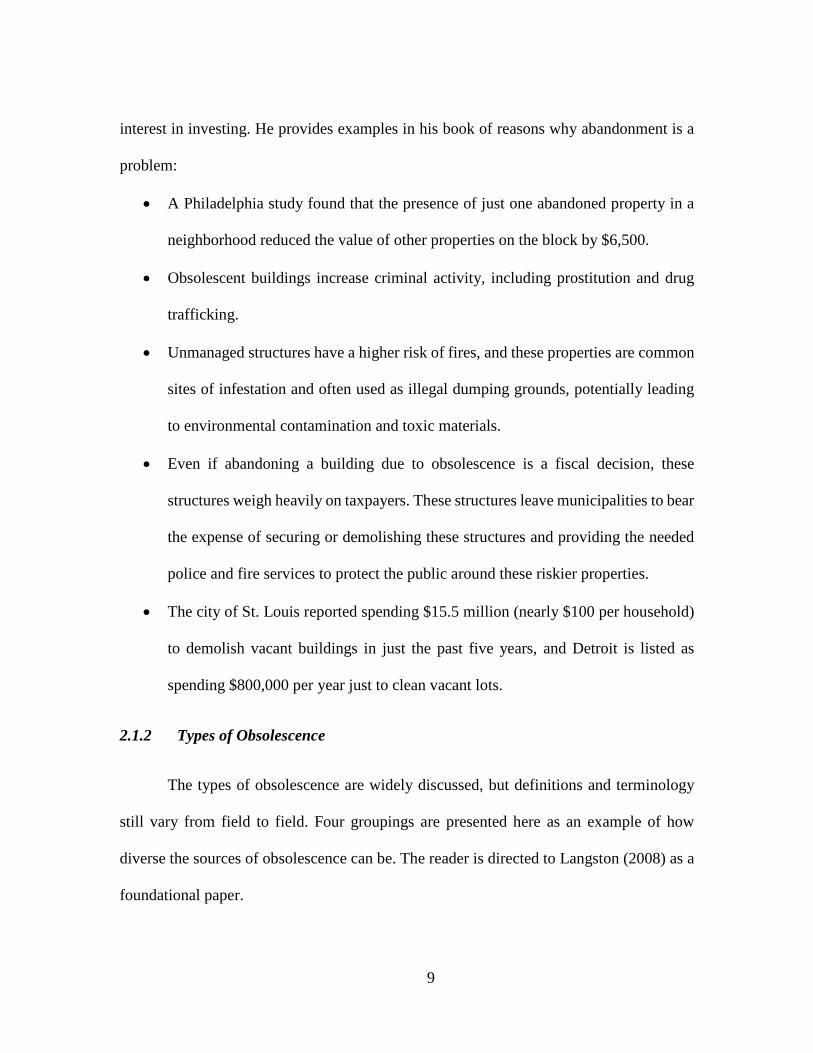
interest in investing. He provides examples in his book of reasons why abandonment is a

problem:

• A Philadelphia study found that the presence of just one abandoned property in a

neighborhood reduced the value of other properties on the block by $6,500.

• Obsolescent buildings increase criminal activity, including prostitution and drug

trafficking.

• Unmanaged structures have a higher risk of fires, and these properties are common

sites of infestation and often used as illegal dumping grounds, potentially leading

to environmental contamination and toxic materials.

• Even if abandoning a building due to obsolescence is a fiscal decision, these

structures weigh heavily on taxpayers. These structures leave municipalities to bear

the expense of securing or demolishing these structures and providing the needed

police and fire services to protect the public around these riskier properties.

• The city of St. Louis reported spending $15.5 million (nearly $100 per household)

to demolish vacant buildings in just the past five years, and Detroit is listed as

spending $800,000 per year just to clean vacant lots.

2.1.2 Types of Obsolescence

The types of obsolescence are widely discussed, but definitions and terminology

still vary from field to field. Four groupings are presented here as an example of how

diverse the sources of obsolescence can be. The reader is directed to Langston (2008) as a

foundational paper.

10

• Functional and/or technological obsolescence (Lemer 1996; Sarja 2005; Kohler

et al. 2010) describes cases where a building is physically insufficient (Richard

Barras and Paul Clark 1996; Wilkinson 2011) to accommodate occupants, such as

having rooms that are too small or have poor sound insulation.

• Legal (Richard Barras and Paul Clark 1996; Wilkinson 2011) and ecological (Sarja

2005) obsolescence occur due to an inability to meet increasing ecological or

environmental requirements, such as pollution, waste production, and

energy/materials consumption standards.

• Economic obsolescence (Sarja 2005) occurs when operation and maintenance costs

are too high in comparison to the cost of building a new facility. Kohler et al. (2010)

reported that demolition rates in Europe are very low, and that the intention to

demolish is often caused by a low rate of return relative to the market value of the

site. A rule of thumb for pursuing demolition is when the costs of renovation exceed

one-third of the cost of a new building.

• Cultural (Sarja 2005), social, and aesthetic (Wilkinson 2011) obsolescence are due

to changes in human satisfaction and style.

There are many more definitions and a plethora of examples of obsolescence in

structures. In fact, many of the obsolescence types given here are referenced by another

name in other texts found in this literature review. This introduction to obsolescence only

serves to provide the reader an idea of its concept, and the provided references direct to

additional reading.

11

2.1.3 Adaptability in Buildings

Adaptability in the built environment can be implemented on many levels to combat

obsolescence. In his book, Stewart Brand describes six shearing layers of a structure, based

on the expected lifetime of each layer (Brand 1995). These “six S’s” are shown in Figure

2.1 with their typical lifetimes. Treating different layers as separate systems is significant

for enabling adaptability in buildings, since this allow us to address different components

of a building on its appropriate time scale. As a preposterous example, if the skin of the

structure were inseparable from the structure, we would be required to demolish the

structure every time we wished to change the color of paint on the walls. Ross et al. (2016)

identifies and summarizes the different strategies of enabling adaptability found in

literature.

Figure 2.1: Layers and lifetimes of structures (adapted from Brand (1995)).

12

There is even potential for adaptability at a scale larger than Brand discusses. The

site of structure exists dependently within a community or city, and adaptability can even

be explored at a regional level. This type of adaptable planning can open up a new field of

study for infrastructure as a whole. City planning of neighborhoods or parks, or even where

to pave roads, may change based on the mindset of city and regional planners. Our choice

to continue building path-dependent structures, often designed to last dozens or even

hundreds of years, can elicit obsolescence quickly when future demands are inevitably

unknown. Ellen Dunham-Jones, professor of architecture and author of “Retrofitting

Suburbia” (Dunham-Jones and Williamson 2011) is a leader in demonstrating the need for

a change in our design thinking to include sustainable practices at the scale of urban

development.

A well-planned example of adaptability in structures is illustrated by the 2012

London Olympics, where the designers of the stadium arenas took possible future needs

and uses of the site into consideration. The designers understood that the Games were a

passing event and could potentially result in a huge waste of infrastructure and investment.

The plan was to convert the 80,000-seat stadium into a regular-sized arena after the Games,

and this was reflected in the use of temporary steel structures which allowed for partial

disassembly. To allow for deconstruction, the stadium had a simple design with only two

parts: a concrete bowl, and a light-weight steel truss structure that comprised the upper tiers

and supported the roof membrane. Even details as small as connections were taking into

consideration for component reuse and adaptability—bolts were used rather than welded

13

steel connections (“London 2012 - Olympic Stadium” 2014). In addition to the stadium,

several other Olympic facilities were designed for adaptability (Feifer 2015):

• the Olympic pool was designed with a floating bottom that can be easily lowered

or raised after construction to meet the needs of Londoners;

• the basketball arena was designed for deconstruction and easy mobility as

basketball is not a popular sport in England; and

• the bridges of the Olympic village were designed as removable platforms, such that

the maintenance requirements after the Games would be appropriate for the normal

population size.

The foresight of the London Olympics designers in creating structures adaptable to

changing demands ensured a prolonged life for both the site and structures by taking the

normal population’s needs into account.

2.1.4 Possible Paths Forward

While there are many research approaches to curbing obsolescence, a few ideas are

listed here.

• Biomimicry, a design method that mimics Nature’s time-tested patterns and

strategies, has potential for teaching us about how to incorporate adaptability

sustainably into our built environment. This approach encourages a shift in our

design paradigm, and its applications are discussed in the following sections.

• Designing for adaptability and deconstruction (DfAD) is a design strategy that

plans for the reuse of building components at the end of a structure’s service life.

14

See Webster (2007) for more details. Incorporating DfAD into our designs would

address adaptability at a component level.

• Teaching adaptability in civil engineering courses can be an educational approach

towards broadening sustainability outcomes. See Chen, Ross, and Klotz (2014) for

an example of a lesson plan and activity where undergraduate students are taught

about the importance of adaptability in the planning stage.

• Adaptability can be encouraged at the decision-making level by smoothing the

process between stakeholders. See Wilkinson (2011) and Wilkinson, Remøy, and

Langston (2014) for details.

• Local communities can be encouraged to reclaim abandoned assets by working

together to repurpose structures. See Mallach (2006) for details.

2.2 Biomimicry Basics

Biomimicry is a design method that draws inspiration from Nature for sustainable

solutions to human challenges. Nature has 3.8 billion years’ worth of time-tested patterns

and strategies, which engineers can learn from and apply; many human problems have

already been faced and resolved in one form or another in Nature. Janine Benyus, the

modern popularizer of biomimicry, describes it as “the conscious emulation of life’s

principles for sustainable solutions” (Benyus, n.d.)—the intention to carefully learn how

to reproduce an effect that both uses and fits within Nature’s principles, creating conditions

conducive to life.

15

“Nature’s principles” refers to the rules of thumb that natural systems follow.

Leading experts have broadly generalized these behaviors into ten principles (Biomimicry

Institute, n.d.), which cover concepts such as an efficient use of energy and resources, the

recycling of all materials, system resilience, and optimization and cooperation, among

others. While certainly not exhaustive, this list gives us a starting point and some clues

towards how to think and design like Nature.

One principle that is of particular relevance for adaptable infrastructure design is

form follows function. While this phrase is widely recognized as originating from modern,

industrial architecture (20th century), this concept draws from the theory of evolution (e.g.,

as described by the overlap in Lamarck and Darwin’s theories in the 16th-17th centuries).

Nature shapes its structural forms to help meet functional requirements, rather than adding

more material and energy to produce similar outcomes (Biomimicry Institute, n.d.). Natural

structures are honed and polished through natural selection, resulting in systems that are

effective, efficient, and multifunctional to meet each organism’s performance demands (D.

A. Chen, Ross, and Klotz 2014b). When abided by, this principle carries potential for a

more sustainable built environment. An introduction to biomimicry in the context of

structures is provided in Chapter 3.

The term bio-inspiration has been popularized in many disciplines, and as the term

suggests, designers often draw qualitative, conceptual ideas from Nature. While

biomimicry suggests an inherent quality of sustainability in a design, bio-inspiration is a

term which encompasses a broader source of creativity (e.g., biomorphism, biophilia, and

bio-utilization, which are all forms of bio-inspiration, but are not intrinsically sustainable)

16

(Bernett 2015). The next step in biomimicry research and practice is to add rigorous

quantitative analysis to justify and support biomimetic designs for sustainability.

As users of biomimicry often function on the border of different disciplines, tools

and databases for connecting ideas between experts is important. The process of using

biomimicry is a two-way street between disciplines, one of them usually being an

engineering field. Biomimicry can be problem-driven, where engineers turn to biology to

search for sustainable ideas, or solution-driven, where scientists try to find an application

for their discovery of interesting phenomenon (e.g., Helms et al. (2008)). Two of the largest

resources for biomimicry are AskNature.org and TRIZ, which are broad databases that

organize organisms by their functions for accessibility to engineers (Vincent et al. 2005).

Many educators have begun to include biomimicry in their coursework, and it appears to

fit well in design engineering curriculums. Reverse engineering a project by using a form-

through-function approach can teach students how to critically think about the objectives

and functions of a design, and substitute sustainable solutions found in Nature (e.g.,

Kennedy, Buikema, and Nagel (2015)).

2.3 Mathematical Characterization and Quantification of Biomimicry

While databases and other biomimicry resources are valuable, this project takes a

different approach towards developing biomimicry into a quantitative tool for engineers.

With an audience of structural engineers, this research considers the natural principle of

form follows function through an engineering lens by exploring natural systems through a

bottom-up approach to reveal system properties of organisms. By pinpointing which

17

emergent properties are the root of structural form, we have the opportunity to create

simplified models of complex systems that are mathematically based. In other words, we

can better understand the mathematical functions underpinning natural forms, and vice

versa. The following sections discuss form follows function in common systems from

various engineering disciplines.

To describe the physical behavior of a system, a mathematical model called a

governing equation is often used (Cha and Molinder 2006). Governing equations are

frequently seen as differential equations obtained by substituting a system’s constitutive

relationships into more general laws of physics. For example, the governing equations of

mechanical systems are expressions of Newton’s Second Law, while those of electrical

systems are representations of Kirchhoff’s Voltage and Current Laws. In these sorts of

analyses, we are primarily interested in a system’s behavioral response to various inputs.

By extrapolating this idea of mathematical description to natural systems, our research

investigates the effect of organisms’ structural parameters on adaptability over time.

2.3.1 Governing Equations of Woodpeckers and Harmonic Oscillators

In classical mechanics, the dynamic motion of a system can be characterized by

three simple elements: a spring, a mass, and a damper. Modeling a mechanical system with

these parameters enables representation of not only its potential energy and energy

dissipation capabilities, but also captures intrinsic characteristics of the system, such as its

natural frequency, and consequently the time it takes return to a steady state response after

a disturbance. Understanding this level of detail is important in many structural

18

applications, as unintentionally vibrating a system at its resonant frequency can cause

catastrophic failure (e.g., Tacoma Narrows Bridge collapse in 1940).

The dynamics of many mechanical systems can be characterized as harmonic

oscillators, which is a system that experiences a displacement and fluctuates around its

equilibrium point. Depending on the values of certain parameters, a system can exhibit

various response behavior. For example, the sole value of the damping ratio (a constant

dependent on the physical specifications of the spring, mass, and damper) can determine

whether the system will return to a steady state value without oscillating past its

equilibrium point, or if the system will return to a stable configuration at all. In cases with

a driving force, oscillation amplitudes may even gradually increase until overwhelming

internal forces cause the system to fail.

Figure 2.2: Simple diagram of (a) spring-mass-damper system; (b) RLC circuit in series

The governing equation of harmonic oscillators is often portrayed as

𝑚𝑚�̈�𝑥 + 𝑐𝑐�̇�𝑥 + 𝑘𝑘𝑥𝑥 = 𝐹𝐹(𝑡𝑡) (1)

where m represents the mass, c is the damping constant modeled as a dashpot and

resists motion via viscous friction, and k is the stiffness of the system modeled as a spring

(Figure 2.2a). By parameterizing a mechanical system in this manner, a space of infinite

19

possibilities of different systems and response behaviors can be created by adjusting either

the element specifications or the input force.

Woodpeckers baffled scientists for some time, as these birds avoided concussions

even with pecking speeds of 6-7 m/s and decelerations of 1000 g (Wang et al. 2011), which

is, conservatively, more than 100 times the acceleration that causes loss of consciousness

in humans (Creer, Smedal, USN (MC), and Wingrove 1960). It has since been discovered

that the woodpecker has a unique musculotendinous tissue as well as spongy bone in its

skull which act as shock absorbers and protect its brain from extreme vibrations (Yoon and

Park 2011). Additionally, the woodpecker has a comparatively long, heavy, and rigid tail,

which it presses against the tree trunk to maintain balance while drumming (Yoon and Park

2011).

The woodpecker can be modeled in elemental form as a spring-mass-damper

system, as its input force and oscillating motion are visible and measurable. When the bird

drives its beak into a tree trunk, the impact energy is dissipated by the bird’s muscles and

unique skull structure (Zhu, Zhang, and Wu 2014), while its rigid tail acts as a spring. Yoon

and Park (2011) illustrate an insightful, simplified (the tail is not included, for example)

mechanical model of the woodpecker’s head structure, and even depict a kinematic model

of the bird during drumming. In the framework of form follows function, the woodpecker

has evolved to have a chisel-like beak (form) for drilling into wood to eat insects (function).

In parallel, its spongy skull bone and rigid tail (forms) aid in protecting the woodpecker

from damage from impact (function).

20

Finite element analysis (FEA) is another engineering tool that has been used to

study organisms. FEA is useful for studying complex behavior and interactions between

various materials and capturing local phenomenon. In addition to the elemental model

discussed above, the woodpecker has also been modeled with FEA for more precise insight

on the dynamic response of its high-impact pecking (Wang et al. 2011; Zhu, Zhang, and

Wu 2014; Oda, Sakamoto, and Sakano 2006).

These biomimetic studies of the woodpecker have led to the development of a new

shock-absorbing system capable of protecting micro-machined devices from large

accelerations and high frequencies caused by mechanical excitations. Inspired by the skull

structure of the woodpecker, this system has a failure rate of 0.7% at 60,000 g, which is

nearly 40 times less than the conventional method, which has a failure rate of 26.4% (Yoon

and Park 2011).

2.3.2 Governing Equations in Other Systems

Table 2.1: Analogous elements between mechanical and electrical systems

Input variable (Effort) Output variable (Flow) Inductance Compliance Resistance force (F) displacement, velocity,

acceleration (𝑥𝑥, �̇�𝑥, �̈�𝑥) mass (m) spring (k) damper (c)

voltage (V) current (i) inductor (L) capacitor (C) resistor (R)

Governing equations are used to characterize non-mechanical systems as well. For

example, similar governing equations are used to characterize electrical systems, in which

parameters are directly analogous to parameters in mechanical systems (see Table 2.1). A

21

diagram of a RLC circuit in series is shown in Figure 2.2b. The governing equation for this

circuit with a constant input voltage has the form

�̈�𝑖+ 𝑅𝑅𝐿𝐿 �̇�𝑖+ 1

𝐿𝐿𝐿𝐿 𝑖𝑖 = 0. (2)

Governing equations are also used in fluid flow and heat transfer, among other

topics. By applying mathematical analysis to natural systems, our aim is similar: to capture

the behavioral response of a system depending on variable input parameters. But instead

of measuring the displacement or resulting current in human-made mechanical or electrical

systems, we aspire to quantitatively understand the behavior of structural growth in natural

systems as environmental factors change. Studying organisms’ forms based on their

“inputs” is a bottom-up approach to biomimicry that may reveal system parameters that

give rise to emergent properties. By searching for the roots of a morphology, we can

discover forms that follow functions that are mathematically based—or, natural forms that

follow mathematical functions.

In this dissertation, engineering mechanics is used to explore the adaptable growth

of a seashell during different stages of its lifecycle. Our research investigates how the

mollusk’s changing functional needs influence the growth in shell formation and how the

system is able to adapt to these changing performance demands.

2.4 Science of Complex Systems

The process of system characterization described above is one subset of complexity

science, which is a field that investigates how individual agents behave collectively to

22

become more than the sum of their parts. The science of complex systems is a broad and

relatively new interdisciplinary field that has rather undefined boundaries, but the amalgam

of research areas provides an idea of what types of complex systems exist. Examples

include physical systems (e.g., molecular matter), ecosystems and biological evolution,

human societies, economics and markets, and pattern formation and collective motion

(Newman 2011). Newman emphasizes that complex systems theory is not a monolithic

body of knowledge and does not believe that a single coherent theory will emerge to

conjoin the variety of existing work. Nevertheless, the topics that tie together this

dissertation have multiple connections to research in complexity science, which can be a

framework to broaden the impacts of this work later on.

23

CHAPTER THREE

LESSONS FROM A CORAL REEF: BIOMIMICRY

FOR STRUCTURAL ENGINEERS

This stand-alone chapter is the manuscript from a forum paper published in the

Journal of Structural Engineering’s April 2015 edition. While this paper uses coral reef as

the running example (rather than shells, which are the technical focus of this dissertation),

this paper presents a summarized background of biomimicry to structural engineers. The

paper is divided by hierarchies in Nature and provides the reader examples of Nature’s

capability of creating structural forms comparable to those used at each scale in traditional

civil engineering. The intention of behind writing this paper was to broadly disseminate

the idea of biomimicry as a potential design enhancement to a technical audience of civil

engineers. By starting the conversation about quantitative biomimicry, we hope to inspire

traditional engineers to seek innovative solutions to the environmental design challenges

we face.

3.1 Introduction: Biomimicry in Practice

Biomimicry is a design concept that draws sustainability and resiliency ideas from

Nature’s time-tested patterns and solutions. The use of biomimetic designs has been

successfully applied to engineering challenges in disciplines such as materials science

(Heintz 2009), fluid dynamics (Saha and Celata 2011), computer science (Ratnieks 2008),

and biomedical engineering (Zhang 2012), among others. Despite this demonstrated

effectiveness in other engineering disciplines, biomimetic research and applications in

24

structural engineering is scarce. There are, however, a handful of architectural designs that

intentionally borrow from Nature. The Eastgate Centre in Zimbabwe mimics Macrotermes

michaelseni (mound-building termites) nests by employing self-regulating heating and

cooling systems through natural air circulation (Biomimicry Institute 2014). Other

examples of using biomimicry to heat and cool buildings include the 30 St Mary Axe

building (nicknamed the “Gherkin”) in London, which imitates the sponge Euplectella

(Venus’ Flower Basket) (Meyers et al. 2008), and Singapore’s Art Center, which has a

building envelope inspired by the way polar bear hairs regulate light and heat absorption

(Horwitz-Bennett 2009).

The objective of this forum paper is to introduce biomimicry to structural engineers

and therefore provide a new jumping off point for related research. Using potential

biomimetic applications of coral reef to the built environment as a running illustrative

example, this paper is intended to help readers seek solutions through their own systematic

investigations of natural forms.

3.2 Design Characteristics Seen in Nature

3.2.1 Form follows function

Wilfredo Méndez Vázquez (Pontifical Catholic University of Puerto Rico)

investigated how structural components might borrow the form of bones. Long bones (e.g.,

femur) grow in a shape that minimizes material while optimizing strength and performance,

and the body naturally builds reinforcement in areas that experience higher levels of stress

(i.e., in areas of muscular growth or at fractures). The typical long bone is thicker at the

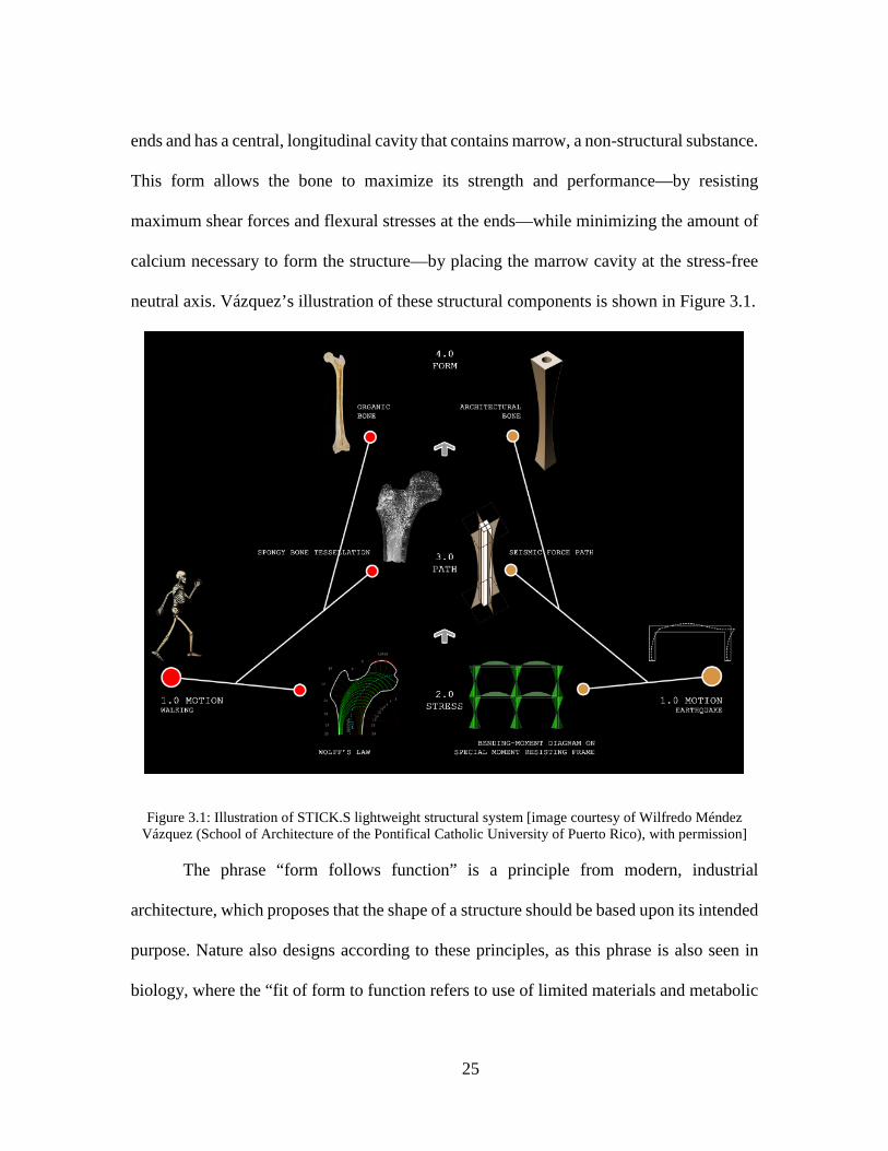
25

ends and has a central, longitudinal cavity that contains marrow, a non-structural substance.

This form allows the bone to maximize its strength and performance—by resisting

maximum shear forces and flexural stresses at the ends—while minimizing the amount of

calcium necessary to form the structure—by placing the marrow cavity at the stress-free

neutral axis. Vázquez’s illustration of these structural components is shown in Figure 3.1.

Figure 3.1: Illustration of STICK.S lightweight structural system [image courtesy of Wilfredo Méndez Vázquez (School of Architecture of the Pontifical Catholic University of Puerto Rico), with permission]

The phrase “form follows function” is a principle from modern, industrial

architecture, which proposes that the shape of a structure should be based upon its intended

purpose. Nature also designs according to these principles, as this phrase is also seen in

biology, where the “fit of form to function refers to use of limited materials and metabolic

26

energy to create only structures and execute only processes necessary for the functions

required of an organism in a particular environment” (Reap, Baumeister, and Bras 2005).

Nature thrives when three characteristics—effectiveness, efficiency, and

multifunctionality—are intricately tied, causing an organism’s structural form to be

dictated by the mutualism of these traits. When Nature designs according to “form follows

function,” structural materials (i.e., resources; primarily the limited availability of organic

elements (Meyers et al. 2008)) are minimized while properties conducive to life (e.g.,

durability and strength) are optimized. Multifunctionality is known as “degeneracy” in

biology: the “realization of multiple, functionally versatile components with contextually

overlapping functional redundancy” (Whitacre and Bender 2013). Similarly, in structural

engineering, an effective design is one that successfully fulfills its intended result (e.g., a

column that maintains stability during an earthquake), and an efficient design achieves

maximum productivity (such as strength) with minimized resources (such as cost and

material). While multifunctionality embodies the principles of effectiveness and efficiency,

it also draws in an aspect of adaptability—a characteristic structural engineers are still

striving towards in the built environment (Kestner, Goupil, and Lorenz 2010). If buildings

are able to achieve mutualism through these three characteristics, we may also be able to

design structures that have optimized forms through their functions.

The Sinosteel International Plaza in Tianjin, China, uses a honeycomb structure

façade to achieve multifunctionality through biomimetic means. While the structure is not

necessarily designed to mimic the functions and features of honeycombs, the hexagonal

structure of the façade (increasing strength) removes the necessity for internal columns

27

(increasing architectural flexibility and material reduction) (Bojovic 2013). Additionally,

each honeycomb cell is positioned and sized accordingly to help with internal temperature

regulation (Etherington 2008). This type of multifunctional biomimicry is a worthy goal.

3.2.2 Lenses of structural hierarchy

Examination of structural hierarchies is a systematic approach commonly used in

the biological and materials sciences to analyze structure-function relationships (e.g.,

Fratzl 2007; Woesz et al. 2011). Structural hierarchy is inherent to all natural forms, and

features found on various scales can help determine the physical properties of materials

and structures (Lakes 1993). However, dimensional scales greatly affect the perception of

and interaction with structural forms, which are often exacerbated by artificial boundaries

between engineering disciplines. This imposed scaling contributes to a divide between

materials (material science), structures (engineering mechanics), and the interaction of

humans with these structures (architecture).

Table 3.1 summarizes categorizations of structural hierarchies found in biomimetic

literature. Of course, as Knippers and Speck (2012) point out, biological structures are built

iteratively through mutation, recombination, and selection; the separation of material and

structure is often impossible. Consequently, the distinctions between the categories in the

table are not always well-defined, and researchers use both strict and loose categories of

hierarchy.

28

Table 3.1: Examples of Structural Hierarchical Categories Found in Literature

Categorization of hierarchy

Example of scales used

Usage Evident in literature

Measurement Ultrascale Nanoscale Microscale Mesoscale Macroscale

Prefixes indicate the physical size of the component (e.g., nanoscale indicates forms that can be measured in nanometers, or microns)

(Meyers et al. 2008) (Knippers and Speck 2012) (Lakes 1993) (Fratzl 2005) (Aizenberg et al. 2005) (Fratzl and Gupta 2007)

Comparative Microscopic Macroscopic Spatially

Terms are used loosely in relation to each other; macroscopic forms are visible to the naked eye, while microscopic ones are not

(Aizenberg et al. 2005)

System/ Manufacturing

Material level Component level Assembly level Product level System level Ecosystem/ Regional level

Perceives the pieces of a structure as subsystems, ultimately contained by the environment

(Reap, Baumeister, and Bras 2005) (Fratzl and Gupta 2007)

Biological processes

Molecular Material Process

Specific towards processes (e.g., energy distribution) instead of structures

(Knippers and Speck 2012)

Contrastingly, our built environment lacks an inherent feedback loop and the

hierarchical processes are dependent on each load-bearing system. In structural

engineering, each system is dependent on the subsystems that comprise it, and this

dependence occurs at each hierarchical level. For instance, the Eiffel tower has three orders

of hierarchy. The L-shaped or rectangular cross-section bars are of the 0th order; the trusses

that are formed by the 0th order bars are of the 1st order; these trusses are then tied together

to form the legs of the tower, which comprise the 2nd order; and the tower in full is

represented by the 3rd order hierarchy (Fazli et al. 2008).

By understanding and comparing the structural hierarchies found in Nature and the

way we design our structures, we are positioned to investigate how these hierarchies lead

to forms that follow their functions and, analogously, how we can design our buildings to

29

do the same. The following discussion on coral reefs helps to translate biology and ecology

terms into a language for structural engineers and demonstrates how a biomimetic

investigation for structural applications can be conducted.

3.3 Translating Coral Reef Characteristics into Engineering Applications

Coral reefs are underwater structures (Figure 3.2) that act as homes to many marine

organisms and are often found a short distance from a coast (see Figure 3.3). Coral reefs

are composed of calcium carbonate, which is deposited through a combination of dead

organisms and wave agitation. Binding material in the reefs comes from attached

occupants, which include the reefs’ namesake as well as other organisms such as mollusks,

worms, and decapod crustaceans (US Department of Commerce 2012). Structural

compositions and forms vary across and within reefs, but generally the reef crest (see

Figure 3.4) protrudes towards incoming waves and disperses some of their energy. Reefs

therefore protect their occupants and can act as a buffer for sensitive coastal regions from

strong waves. Coral reefs can decrease tsunami run-up—a temporary rise in sea level,

measured in meters above a reference sea level (US Geological Survey 2008)—on the order

of 50%. Reefs can also decrease the energy of wind-driven waves by at least 80% (Kunkel,

Hallberg, and Oppenheimer 2006).

30

Figure 3.2: Collection of coral on the Great Barrier Reef (image courtesy of Wikimedia Commons/Toby Hudson)

Figure 3.3: Aerial view of the Great Barrier Reef off the coast of Australia (image courtesy of NASA)

31

Figure 3.4: Diagram indicating regions of the reef, including the reef crest (diagram courtesy of NOAA)

Using the previously discussed structural hierarchy of natural forms, we can learn

biomimetic lessons from the coral reef on five scales:

1. Material Scale: Composition and Material Properties of the Reef Substrate

2. Component Scale: Mechanical Properties of the Coral Skeleton

3. System Scale: Components of the Reef

4. Spatial Scale: Mutualism of Reef Components

5. Regional Scale: Reef Dimensions and Distance to Shore

Again, the separation between levels is useful for analysis, but also imprecise due

to the organic adaptability of natural forms, as will be evident through the discussion.

3.3.1 Material Scale: Composition and Material Properties of the Reef Substrate

Material properties of the reef substrate vary across different parts of the reef, which

is comprised of the skeletons of coral polyps (see Figure 3.5) and other attached

microorganisms. Less turbulent wave motion between the reef’s crest (initial impact) and

32

back (final dissipation) results in more consistent depositions of new substrate resources

into reef gaps, causing more organic diversity in these areas (J. S. Madin et al. 2012). Areas

with more calcium carbonate deposits lead to higher degrees of cementation and, therefore,

density, which is the main correlate with the strength of the material. Structural designers

know this positive correlation between density and strength is common in building

materials (Chamberlain 1978). For example, the ACI 318 code for structural concrete

includes empirical factors to account for reduced strength in members made with

lightweight concrete (ACI Committee 318 2011).

Figure 3.5: Various components of a coral polyp situated on a coral reef

Due to the relatively high porosity of the coral skeleton, its skeletal material is

weaker than that of most other organisms’ skeletons and also does not absorb strain energy

as well, being prone to fracture. Still, coral skeleton, a main component of coral reefs, has

a strength comparable to engineering building materials, such as concrete, while using less

material per unit volume, as shown in Table 3.2 (Chamberlain 1978). Chamberlain also

found that the stress-strain relationship for coral skeleton is effectively linear and that the

skeleton has a low ultimate strain, meaning coral skeleton is a linearly elastic material.

33

Structural design engineers could use coral’s comparable strength as motivation in

redesigns of human-made materials, such as concrete, to be stronger while using less

material. The result would be a substance that is not only lighter, but also has less embodied

energy and is easier to construct.

Table 3.2: Coral Skeleton Properties Compared to Engineering Building Materials

Category Material Strengtha (MNm-2)

Porositya,b Elastic Modulus (GNm-2)

Density (g cm-3)

Coral skeleton 12-81 0.3 2-38a 0.82-2.41c

Vertebrates Human cancellous bone 4 0.5 0.1-4.5d 1.08e

Human compact bone 210 9 17f 1.85e

Engineering Materials

Granite 52 0.01 52 2.6-2.8 Concrete 32 0.12 25c 2.32c

Steel 800 0 200c 7.86c

Aluminum 600 0 70c 2.71c

aAdapted from Chamberlain (1978). bPorosity = pore volume/ total volume of material. cData from Hughes (1987). The ranges of densities shown correlate to the coral species tested in Chamberlain

(1978). dVaries depending on the bone density and trabecular orientation, from Turner et al. (1990). eMean density of fresh bone from Blanton and Biggs (1968). fData from Reilly and Burstein (1975).

3.3.2 Component Scale: Mechanical Properties of the Coral Skeleton

Chamberlain also tested the skeletal fracture patterns of various types of coral

(Figure 3.6) and found that the skeletal cores of three coral species were all strongest when

compressive forces were applied parallel to the direction of the grain— demonstrating a

similarity to other anisotropic materials such as bone and wood. This experiment also

showed that the strength of the skeleton varies inversely with the skeletal porosity. In other

words, sections of the coral that are more porous are also weaker. Remarkably, the coral’s

adaptive nature allows for it to decrease its porosity by augmenting skeletal growth in areas

that experience higher stresses to increase its strength in these locations. Indeed, a

difference in both porosity and strength are observed between smaller but more highly

34

stressed coral branches and other larger but only moderately stressed forms. This

observation in coral could remind designers that in addition to matching various materials

to structural functions, density of human-made materials as a function of its position in a

structure is an overlooked parameter that can be altered.

Figure 3.6: Various coral skeletal cores and their fracture patterns (adapted from Chamberlain (1978))

Coral’s replenishment of skeletal material where needed is similar to the previously

discussed regeneration of fractured human bones, a process that can inspire the

development of smart structures that learn from and adapt to past load demands. This

replenishing ability is observed within the lifetime of the coral, but coral have also

developed intergenerational evolutionary advantages, as discussed next.

3.3.3 System Scale: Components of the Reef

J. S. Madin’s study (2005) of the mechanical limitations of reefs shows how

strength variations between different types of coral may be an evolutionary development

in those with structural forms prone to fracture due to hydrodynamic forces. Reefs are

35

inhabited by corals of various shapes and sizes (see Figure 3.7), and coral skeletons with

more protrusions are more likely to have their branches damaged or dislodged. Madin’s

work shows that these damage-prone coral have evolved to develop superior strengths. In

essence, components’ designs have evolved to carry anticipated loads, which is a frequent

design objective of structural engineers. Through evolution, however, coral have more

practice “designing” forms than even the most experienced engineers. Coral skeletons are

able to gauge and experience the stresses induced by their environment and grow and adapt

to withstand these over generations, resulting in specific morphologies that are naturally

stronger than others.

Figure 3.7: Morphologies of some coral species (adapted from Madin (2005))

While human-made materials do not typically grow organically, this biomimetic

principle can still be used to develop adaptable materials. For example, the biomimetic

Flectofin® is a kinetic and pliable flapping device that changes its shape depending on the

loads it experiences, much like the Strelitzia reginae flower (Bird of Paradise). The stamen

of the Bird of Paradise (see Figure 3.8) is an ideal perch for feeding birds, and the weight

of the bird pushes the stamen downwards, opening the fused petals to expose the flower’s

pollen. The Flectofin® similarly transforms based on applied loads and exploits the

36

potential of asymmetrical bending motion with multiple deflected equilibrium points to

attain a reversible deformation (Lienhard et al. 2011). The Flectofin® shows that there are

still ways to design for adaptability even using traditional building materials that do not

grow organically after they are put into use.

Figure 3.8: Strelitzia reginae: (left) without; (right) with pollen exposed (images courtesy of Phil Gates, http://digitalbotanicgarden.blogspot.com, with permission)

For structural engineering in particular, a future application for smart materials may

be to develop a structure that uses a feedback loop similar to the one observed in the coral

reef. The loop could routinely increase material density to strengthen the structure in

necessary areas. Such applications would be especially beneficial as structures increasingly

face changes in demand due to urbanization, climate change, and other foreseeable and

unforeseeable impacts.

3.3.4 Spatial Scale: Mutualism of Reef Components

As discussed above, the coral skeleton may not be the strongest structural material,

but strength is not always a functional requirement in the reef. In fact, the need for strength

37

is contradicted by competing adaptive requirements for a thriving coral reef (Chamberlain

1978), as seen in the emergent properties at the spatial scale.

Coral reefs balance skeletal strength with locational adaptability. As Chamberlain

(1978) found, spatial needs of soft coral may in some cases prohibit the growth of strong,

low porosity skeletons. Or, unusually strong skeletons may inhibit the dislodgement and

distribution of dead coral fragments, which are crucial for the reef to replenish its structure.

Finally, some coral may not require strong skeletons if the probability of their breakage in

their area is low. In essence, increasing structural strength is not always advantageous or

favorable.

Current infrastructure challenges are exacerbated by the sheer amount of

demolitions due to building obsolescence (“Minnesota Demolition Survey: Phase Two

Report, Prepared for: Forintek Canada Corp.” 2004). As coral reefs have evolved to adapt

to changing conditions, engineers can look for similarly appropriate, adaptable solutions to

changes in the built environment. Unnecessary demolitions may be avoided if lessons can

be learned from the coral reef. Building components can be designed for reuse in other

structures (“Design for Deconstruction” 2010) and adaptability can become a spatial scale

criteria for infrastructure.

3.3.5 Regional Scale: Reef Dimensions and Distance to Shore

Through an even wider lens in the hierarchy of natural forms, we see the

effectiveness of the reef as a buffer as a function of its distance to land. Kunkel, Hallberg,

and Oppenheimer (2006) quantified the importance of different reef parameters; such as

38

width, offshore distance, and health; in blocking tsunami energy. Generally, the broader

and shallower the reef, the more protection it provides to the shore. However, if a reef is

too close to shore, it becomes ineffective against longer tsunamis since its relative location

does not allow for significant dissipation of tsunami energy.

The wavelength of incoming currents also plays a role in the effectiveness of the

reef: longer wavelength and larger tsunamis can overwhelm the buffering service of the

reef. Studying buffer characteristics of the coral reef at the regional scale could inform site

selection of coastal piers and jetties. The form of these structures can be enhanced by

incorporating the dimensional properties of the most effective coral reef buffers. Coastal

engineers have, in fact, studied and incorporated wave information into mathematical

design guidelines based on empirical methods (Rosati 1990), and some of this research has

even been implemented in existing coastal structures. Applying a biomimetic design

approach is a more recent development (Curwood and Frankic 2012).

3.4 Conclusions

The analysis of coral reefs shows the potential of applying biomimicry to structural

engineering at various levels of a natural hierarchy. For example:

• Coral skeletal material has strengths similar to human-made building materials,

despite a greater porosity. Biomimicry could lead us to building materials with

improved strength-to-weight ratios.

• Coral skeletons adjust their porosity based on reef location and areas of high stress.

Biomimicry reminds us that the density of manufactured materials as a function of

39

its position in the structure can be altered to enhance performance. Similarly,

biomimicry can lead to advances in smart materials that adapt to their surroundings.

• The coral reef has evolved to exercise appropriate, adaptable behavior for its own

benefit. Biomimicry to inform design of reusable building components and

assemblies can prevent unnecessary demolitions due to building obsolescence.

• Coral reefs’ spatial relationships with their surroundings could improve the

buffering effectiveness of shoreline stabilization structures, such as jetties and

breakwaters. Biomimicry considering climate and wave patterns can lead us to

more effective, culturally-, and environmentally-appropriate structures.

These are just examples of how a systematic, hierarchical approach can provide

biomimetic insights. The suggested potential applications from coral reefs are a guide to

help readers towards their own ideas. Speculated applications likely require collaboration

with adjacent disciplines, such as materials science and mechanical engineering, as natural

forms do not obey artificial disciplinary boundaries. As advocated by groups like the

National Research Council, some of the biggest opportunities for scientific advances are at

the convergence of multiple disciplines (National Research Council et al. 2014). Applying

biomimicry to structural forms can put structural engineers at the leading edge of these

advances.

Researchers and practitioners can contribute to a new generation of biomimetic

solutions in structural engineering. Currently, many designers turn to Nature for

qualitative, conceptual ideas, but the next step is to demonstrate both qualitative inspiration

and quantitative analysis. The structural engineering community has the tools to investigate

40

organisms with biomimetic potential using modeling techniques ranging from single

degree-of-freedom, constitutive models to detailed, finite element modeling of natural

forms. A bottom-up approach like this could reveal system properties of the organism that

give rise to emergent properties that may be the root of the function causing structural form.

By testing these models against their biological counterparts for their capacity of resisting

forces, deformations, and accelerations, we can discover forms that follow functions that

are mathematically based, or, in other words, natural forms that follow mathematical

functions.

41

CHAPTER FOUR

SHELLS IN LITERATURE

“Shells” can refer to a multitude of concepts, depending on the discipline the

terminology is found in. The interdisciplinary nature of this project necessitates an

introduction to the usage of different terms in each context. This chapter covers the

ecological background of mollusk shells, including how their environmental conditions

have led to certain evolved characteristics; a literature review of the computational

modeling of gastropod shells, which is the foundation for this dissertation; as well as an

explanation of classical shell mechanics as found in traditional civil engineering.

Understanding the ecological background of organisms is important for appropriate and

thorough biomimicry, as environmental conditions can be fundamental causes for specific

evolutionary traits. This scientific understanding helps to inform the model-building, which

can be used to simulate the organism in its natural environment, including external forces

acting upon it such as predators or fluid flow. “Shells” in engineering mechanics, on the

other hand, describes a three dimensional structure with a thickness that is small relative to

its other dimensions; many overlaps between shells in engineering and shells in biology

are apparent.

4.1 Biology of Gastropods

This section covers some of the basic terms used to describe shells, leaving Section

4.2 to describe the mathematical variables ascribed to the geometry and growth of the shell.

The spiraled gastropod shell follows a simple growth pattern and is able to adapt its

42

structure to changing performance demands (its increasing snail size). While “enlarging”

is likely one of the more simple forms of growth, this project is an early attempt at

characterizing adaptability in natural systems.

This project uses the Turritella terebra gastropod as its focus. The biological

background and the computational modeling are based on this species, and more generally

on spiraled gastropods, when necessary. The T. terebra was chosen for its small size and

convenience as a sample, and also due to a few studies in literature that show successful

modeling of the gastropod species (e.g., Sorguç and Selçuk (2013)).

4.1.1 Ecology and Evolution of T. Terebra

T. terebra is a species of the Gastropoda class, which is a category of Mollusca, a

taxonomic phylum in terms of scientific classification. Shelled gastropods are commonly

referred to as “snails”, and most gastropod shells are spirally coiled. The T. terebra is

sometimes called the screw turret, screw shell, or great screw shell, and is found in the

Indo-West Pacific, a region spanning the tropical waters of the Indian Ocean and western

and central Pacific ocean (Hardy 2016). Curiously, photos of living Turritella snails appear

to be non-existent, and the live animal is yet to be encountered on shores (Tan 2008).

However, Figure 4.1 shows a drawing of what the snail may look like through its close

relative, the Turritella plebia (Calvert Marine Museum 2016).

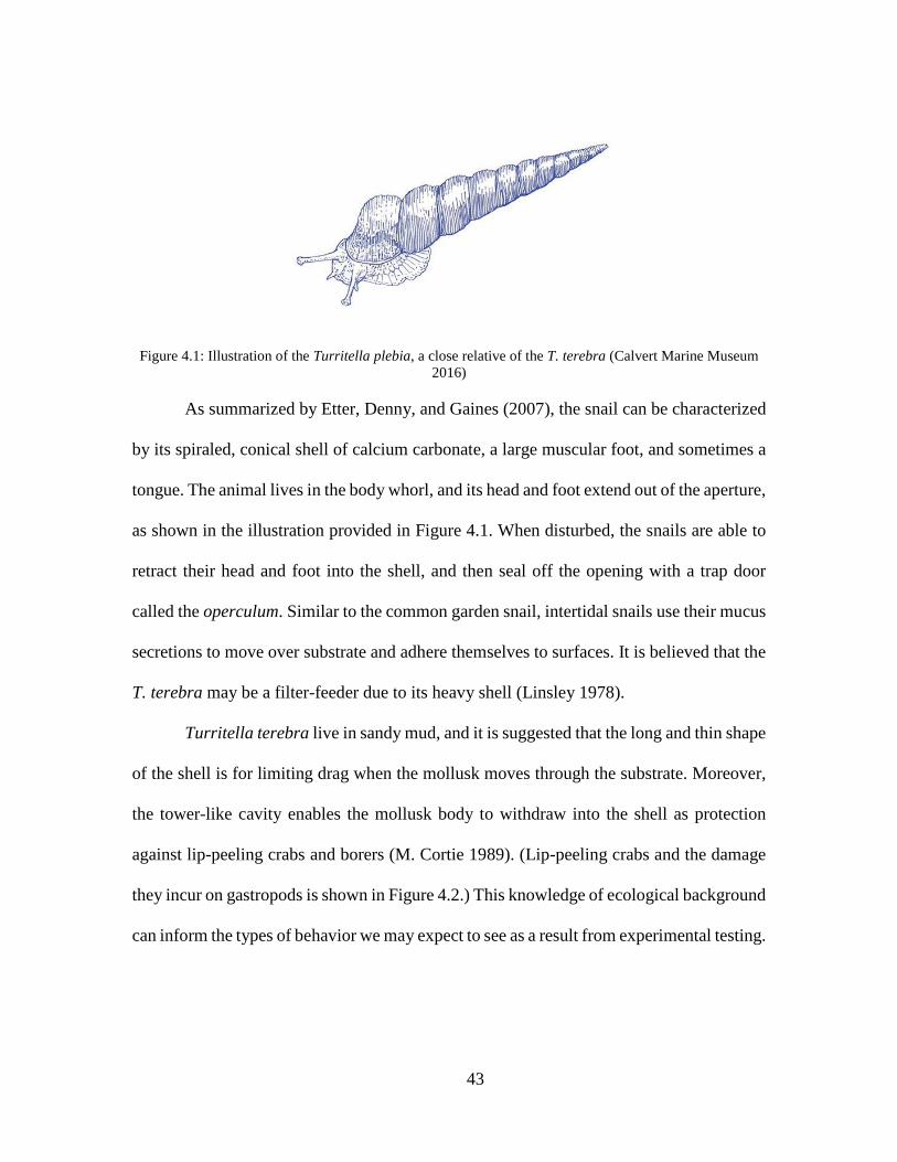
43

Figure 4.1: Illustration of the Turritella plebia, a close relative of the T. terebra (Calvert Marine Museum 2016)

As summarized by Etter, Denny, and Gaines (2007), the snail can be characterized

by its spiraled, conical shell of calcium carbonate, a large muscular foot, and sometimes a

tongue. The animal lives in the body whorl, and its head and foot extend out of the aperture,

as shown in the illustration provided in Figure 4.1. When disturbed, the snails are able to

retract their head and foot into the shell, and then seal off the opening with a trap door

called the operculum. Similar to the common garden snail, intertidal snails use their mucus

secretions to move over substrate and adhere themselves to surfaces. It is believed that the

T. terebra may be a filter-feeder due to its heavy shell (Linsley 1978).

Turritella terebra live in sandy mud, and it is suggested that the long and thin shape

of the shell is for limiting drag when the mollusk moves through the substrate. Moreover,

the tower-like cavity enables the mollusk body to withdraw into the shell as protection

against lip-peeling crabs and borers (M. Cortie 1989). (Lip-peeling crabs and the damage

they incur on gastropods is shown in Figure 4.2.) This knowledge of ecological background

can inform the types of behavior we may expect to see as a result from experimental testing.

44

Figure 4.2: (a) Lip-peeling crabs and pincers (Rosales 2002); (b) gastropod shell damage caused by crab (Whitenack and Herbert 2015)

Shelled gastropods are born with a protoconch, which is the part of the shell that

develop as a coil in embryo. As the snail grows, the living animal is capable of secreting a

substance (from its soft mantle tissue) which solidifies to deposit material at the edge of

the shell opening (Hutchinson 1989). This gradual deposition of primarily calcium

carbonate connects the current revolution to the previous shell section, creating sutures.

The build-up of material creates and lengthens the spire over time.

4.1.2 Terminology of the Gastropod Shell

General terminology of the gastropod shell is labeled in Figure 4.3. The aperture is

the opening of the body whorl at the base of the shell, where the mollusk lives. Material is

added to the edge of the aperture as it grows, developing the spire over time. The columella

is (boxed in red in Figure 4.3) is the axis that develops as whorls (a full revolution of the

45

spiral) begin to impinge on one another. As the height and the diameter of the base increase

through growth, the apex (tip) of the shell moves farther away from the mollusk’s body.

Figure 4.3: Terminology of the Turritella terebra shell features

Some species of gastropods have looser coils that result in a hollow conical space

in the central axis. This hollow axis is called an umbilicus (the navel) and can be perceived

as the opposite phenomenon of columella development. Figure 4.4 shows the different

standard views of a spiraled shell; if the shell has an umbilicus, it would be visible in the

basal view (Figure 4.4d).

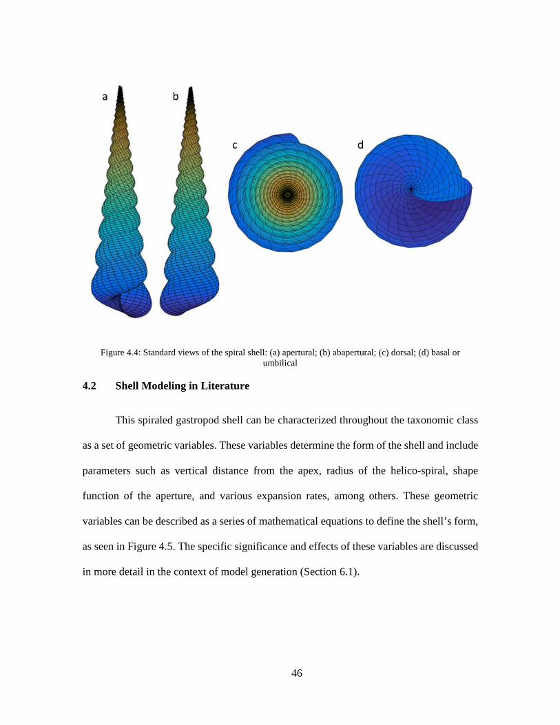
46

Figure 4.4: Standard views of the spiral shell: (a) apertural; (b) abapertural; (c) dorsal; (d) basal or umbilical

4.2 Shell Modeling in Literature

This spiraled gastropod shell can be characterized throughout the taxonomic class

as a set of geometric variables. These variables determine the form of the shell and include

parameters such as vertical distance from the apex, radius of the helico-spiral, shape

function of the aperture, and various expansion rates, among others. These geometric

variables can be described as a series of mathematical equations to define the shell’s form,

as seen in Figure 4.5. The specific significance and effects of these variables are discussed

in more detail in the context of model generation (Section 6.1).

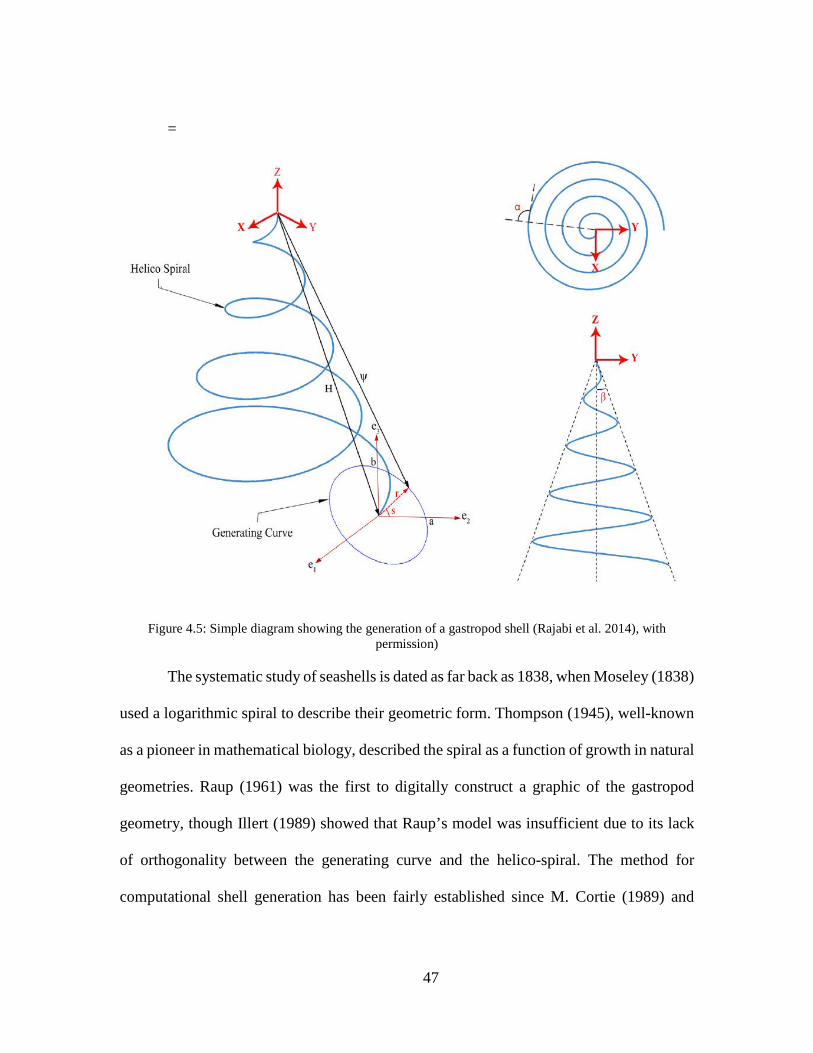
47

=

Figure 4.5: Simple diagram showing the generation of a gastropod shell (Rajabi et al. 2014), with permission)

The systematic study of seashells is dated as far back as 1838, when Moseley (1838)

used a logarithmic spiral to describe their geometric form. Thompson (1945), well-known

as a pioneer in mathematical biology, described the spiral as a function of growth in natural

geometries. Raup (1961) was the first to digitally construct a graphic of the gastropod

geometry, though Illert (1989) showed that Raup’s model was insufficient due to its lack

of orthogonality between the generating curve and the helico-spiral. The method for

computational shell generation has been fairly established since M. Cortie (1989) and

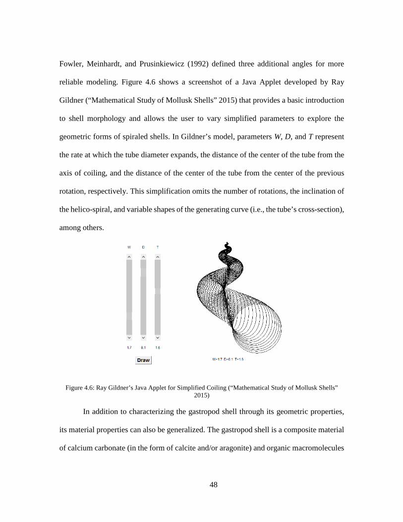
48

Fowler, Meinhardt, and Prusinkiewicz (1992) defined three additional angles for more

reliable modeling. Figure 4.6 shows a screenshot of a Java Applet developed by Ray

Gildner (“Mathematical Study of Mollusk Shells” 2015) that provides a basic introduction

to shell morphology and allows the user to vary simplified parameters to explore the

geometric forms of spiraled shells. In Gildner’s model, parameters W, D, and T represent

the rate at which the tube diameter expands, the distance of the center of the tube from the

axis of coiling, and the distance of the center of the tube from the center of the previous

rotation, respectively. This simplification omits the number of rotations, the inclination of

the helico-spiral, and variable shapes of the generating curve (i.e., the tube’s cross-section),

among others.

Figure 4.6: Ray Gildner’s Java Applet for Simplified Coiling (“Mathematical Study of Mollusk Shells” 2015)

In addition to characterizing the gastropod shell through its geometric properties,

its material properties can also be generalized. The gastropod shell is a composite material

of calcium carbonate (in the form of calcite and/or aragonite) and organic macromolecules

49

(e.g., proteins). A handful of researchers have contributed to the identification of the

material properties of various gastropod shells (e.g., Neves and Mano 2005; P.-Y. Chen,

McKittrick, and Meyers 2012). Table 4.1 shows the range of values for mechanical

constants for the Otala lactea (the Spanish snail) as summarized by Rajabi et al. (2014).

Table 4.1: Mechanical properties of O. lactea as summarized by Rajabi et al. (2014)

Property Value References Young’s modulus 30-68 GPa Currey, 1976;

Currey and Taylor, 1974; Kearney, 2006

Shear modulus 19-39 GPa Kearney, 2006 Bulk modulus 47-69 GPa Kearney, 2006 Tensile strength 25-60 MPa Currey, 1976;

Currey and Taylor, 1974 Compressive strength 198-336 MPa Currey, 1976;

Liang et al. 2008 Shear strength 22-36 MPa Kearney, 2006 Fracture energy 157.7 N/m Ashby et al., 1995 Density 2800 kg/m^3 Ashby et al., 1995 Poisson’s ratio 0.3 Karmat et al., 2004

Researchers have even gone on to structurally model gastropod shells, as this

project does for the Turritella terebra. Mathematical models such as the ones described

above have been expanded into 3D computational models (Faghih Shojaei et al. 2012;

Jirapong and Krawczyk 2003), and a handful of researchers have even incorporated

material properties and applied loads to finite element models to determine the stress and

failure profiles of various shell geometries (Faghih Shojaei et al. 2012; Rajabi et al. 2014;

Sorguç and Selçuk 2013).

The fascinating geometry of shells has attracted interest in all sorts of

disciplines for different purposes, which leads to a large body of literature in the

characterization of these organisms. Table 4.2 organizes some of the literature by the

50

research goal and applications to show the breadth of available information. As

demonstrated by the variety of researchers, this project continues an ongoing pursuit of

scientific understanding and illustrates both the support and impact this body of work can

have.

Table 4.2: Some examples of shell research, sorted by researcher objective and applications of their work

Goal Application Literature Review

Shell geometry characterization

Paleontological reconstruction of shell structures

Thompson, 1945 Raup, 1961 Prusinkiewicz and Steribel, 1986 Cortie, 1993

Shell geometry modeling Mathematical exploration of natural forms Architectural study of natural forms

Picado, 2009 Jirapong and Krawczyk, 2003

Growth pattern characterization (e.g., ridges, pigmentation patterns)

Artistic generation of precise shells

Picover, 1989 Fowler, Meinhardt, and Prusinkiewicz, 1992 Boettiger, Ermentrout, and Oster, 2009

Biomechanical exploration of nacre

Material characterization Mechanical behavior of biological materials

Currey and Taylor, 1974 Currey, 1976 Yang, 1995 Neves and Mano, 2005 Neves and Mano, 2009 Rim et al., 2011 P.-Y. Chen, McKittrick, and Meyers, 2012

Structural analysis of shell model

Numerical technique Faghih Shojaei et al., 2012

Study of mechanical behavior for bio-inspired materials

Rajabi et al., 2014

Spire design in architecture Sorguç and Selçuk, 2013

Parametric analysis of morphology

Furthering molluscan studies Cortie, 1989

51

4.3 Classical Shell Mechanics

A project on shells using engineering mechanics would be folly to leave out

remarks on classical shell mechanics. The theory of shell mechanics is, simply put, an

explanation of how to find a series of equations to solve for static equilibrium in shells.

“Shells”, in the engineering mechanics sense, refers to a thin-walled structural element with

some curvature, where the thickness of the transverse element is small in comparison to

the element’s principal radii of curvature (i.e., 𝑡𝑡𝑟𝑟≪ 1).

Take the standard infinitesimal element with volume (𝑑𝑑𝑥𝑥)(𝑑𝑑𝑑𝑑)(𝑑𝑑𝑑𝑑), commonly

seen in an introductory statics courses, in which we study changes in stress as we sum

forces in the three directions. Considering both normal and shear forces, and by

implementing constitutive laws, we solve for the unknown variables given equilibrium,

Hooke’s law, and strain-displacement equations. If one dimension is much smaller than the

others, this hypothetically cube-shaped element is approximated as a thin plate. Then, thin

shells are simply thin plates with curvature; however, it is important to note a difference

when subjected to external loading. A plate element in equilibrium is only possible under

bending and twisting moments accompanied by shear forces, but a shell element is able to

transmit surface loads through membrane stresses (Timoshenko and Woinowsky-Krieger

1959).

While the theory of shells can become complex quickly, in the end, it is no more

than following the same pattern (as in statics problems) of applying unique boundary

conditions to a sum of forces and moments, and substituting constitutive equations to

obtain a closed-form solution. This approach (which, by the way, involves some complex

52

differential equations) is easily grouped with the concept of governing equations as

described in Section 2.3; this is again a case of applying laws of physics to understand

unique situations. In regards to the use of this mechanics theory in modeling the seashell,

two main reasons for its omission are given:

1. Timoshenko demonstrates in his canonical text (1959) that, in the case of thin

shells, the ratio of bending stresses to membrane stresses is small, and the use of

membrane theory as a first order approximation is justified for shell structures. In

principle, membrane theory is independent of bending, necessitating bending

discrepancies to be considered in the elements’ edge zones. This project,

contrastingly, is particularly interested in the global effects of bending.

2. The theory for shells and membrane is given for simple geometries (e.g., spheres,

rings, domes) and there is little guidance nor much sense in attempting to manually,

numerically model a complex spiraling structure with overlapping shell walls and

changing thicknesses.

In fact, concerning the second point above, there is software developed specifically

for this purpose. Modeling software such as ANSYS and ABAQUS use the finite element

(FE) method (or FEM) to numerically approximate solutions to boundary value problems

– problems in which a solution to the differential equations also satisfies the boundary

conditions (e.g., loads and constraints) acting upon the object. FEM divides the object into

small elements, like the ones used in statics problems described above, and solves an

assembly of these simpler elements in a larger system of equations for a combined global

equilibrium. This project uses ANSYS FE software to structurally analyze the T. terebra

53

shell and observe global effects, such as load paths, failure modes, and shell deformation.

The details of this FE model are provided in Chapter 6.

54

CHAPTER FIVE

EMPIRICAL AND EXPERIMENTAL DATA

This chapter is divided into two main sections describing, first, measurable and

observable characteristics of the sample population and, second, recorded results from

experimental testing.

5.1 Empirical Data

A collection of Turritella terebra shells was purchased in bulk from an online

vendor, Seashellcity.com, which has a physical store in Delaware. A total of 202 shells

were obtained, roughly divided by the vendor into two groups of 3-4 inches and 5 inches

in total length. Upon further request, some limitations were brought to attention, including

a lack of information about when or where the specimens were collected and any details of

the cleaning, storage, or handling. (Sea Shell City representatives were, however, able to

share that their T. terebra shells are generally found off the coasts of India and the

Philippines.) While the missing information is important to note, it does not preclude the

rest of this study.

A series of measurements were taken to collect information about the physical

characteristics of the sample population, including height, base width, and mass. Some

measurements, such as density and thickness, involved physical alteration of the specimens

as a prerequisite. The following sections describe the process and results of these simple

measurements.

55

5.1.1 Height and Width

Upon receipt of the specimens, a handful of samples were experimented on out of

curiosity (and “damaged”, for all intents and purposes) before measurements were taken.

The heights and base widths of the remaining population of 197 shells are displayed in the

histograms below.

Due to the irregular shape of the shells, these measurements are all approximate but

still provide a good representation of the distribution of shells (e.g., as opposed to a digital

measurement of the tip-to-base length at the mid-plane cross-section). The samples were

measured by eye to within 1/16-inch using a standard 12-inch ruler. Heights1 were

measured from the apertural view, starting at the tip and ending at the furthest edge of the

aperture; and the diameters were measured from the basal view at the widest point (see

Figure 5.1).

Figure 5.1: Diagram of measurement convention for (a) sample height and surrogate angle βo in apertural

view and (b) sample width in basal view

1 Height and length are sometimes used interchangeably throughout this dissertation. While the terminology suggests different orientations of the shell, both terms are the measurement of the shell along its columella axis as an increasing distance from the tip.

56

Figure 5.2: Histograms of heights (top) and base diameters (bottom) of sample population

As illustrated in Figure 5.2, the histograms for height and base diameter do not

demonstrate obvious normal distributions. This abnormal distribution is likely due to the

sorting method of the seashell vendor, in which the only categories were “3-4 inch” shells

0

5

10

15

20

25

30

Num

ber o

f sam

ples

Total shell height (in)

Histogram of shell heights

0

10

20

30

40

50

60

Num

ber o

f sam

ples

Max shell diameter

Histogram of shell diameters

57

and “5 inch” shells, with no other details provided. Figure 5.3 below shows the linear

relationship of base diameter to total height, taking all shell sizes into account.

Figure 5.3: Relationship of base diameter to total height of all shell sizes

From these two dimensions, a surrogate angle of expansion can be roughly

calculated, which is named 𝛽𝛽𝑜𝑜 in reference to the angle 𝛽𝛽 described by Faghih Shojaei et

al. (2012) and discussed in Section 6.1. This surrogate property 𝛽𝛽𝑜𝑜 measures the angle

between the central axis and the outer wall of shell from an apertural view (Figure 5.1a). It

should be noted that this angle is used only for referencing the relative sizes of shell

specimens, as there are a variety of factors that preclude its usefulness. For instance, while

the walls of the shells thicken as the total length of the shell increases, this changing

thickness is not accounted for in the measurement of 𝛽𝛽𝑜𝑜. Thus, this surrogate angle of

expansion merely approximates the tangent of maximum width-to-maximum height and

does not take into account the more intricate features of the shell. Interestingly, even though

𝛽𝛽𝑜𝑜 is based on two different groupings of shell sizes, the histogram of 𝛽𝛽𝑜𝑜 reveals a normal

y = 0.1441x1.302

R² = 0.7102

0.4

0.6

0.8

1

1.2

1.4

1.6

4 4.2 4.4 4.6 4.8 5 5.2 5.4 5.6

BASE

DIA

MET

ER (I

NCH

ES)

HEIGHT (INCHES)

FINAL BASE DIAMETER VS. FINAL HEIGHT

58

distribution of all sample sizes (shown in Figure 5.4). In addition, Figure 5.5 shows the

scatter of the sample population of 𝛽𝛽𝑜𝑜 as function of height and base diameter.

Figure 5.4: Histogram of βo across all shell sizes

05

101520253035404550

4 5 6 7 8 9 10

Freq

uenc

y

Degrees

Histogram of 𝛽𝛽𝑜𝑜(outer wall angle of expansion)

59

Figure 5.5: Relationship of βo to total height (top) and base diameter (bottom)

5.1.2 Shell Size vs. Shell Age

Following the description of the height and widths of the sample population, a note

on shell size versus shell age is necessary before further discussion. In the following work,

the shells are grouped in two ways: by “size” and “age.” The three categories for “size” are

small, medium, and large, where small shells are those with total heights of 3.0-4.0 inches,

y = 0.4507x + 4.4655R² = 0.2427

3.5

4.5

5.5

6.5

7.5

8.5

9.5

3 3.5 4 4.5 5 5.5 6

ANGL

E (D

EGRE

ES)

HEIGHT (INCHES)

𝛽𝛽𝑜𝑜 VS. HEIGHT

y = 2.2586x + 4.1754R² = 0.6044

3.5

4.5

5.5

6.5

7.5

8.5

9.5

0.4 0.6 0.8 1 1.2 1.4 1.6

ANGL

E (D

EGRE

ES)

BASE DIAMETER (INCHES)

𝛽𝛽𝑜𝑜 VS. BASE DIAMETER

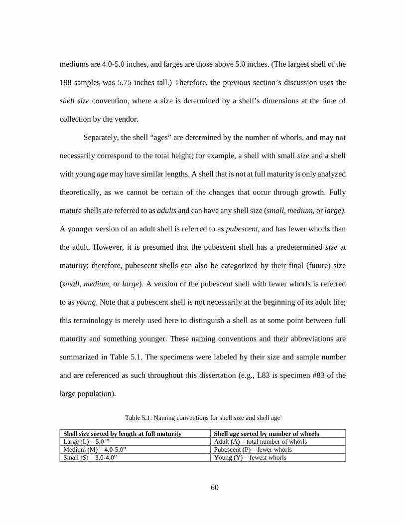
60

mediums are 4.0-5.0 inches, and larges are those above 5.0 inches. (The largest shell of the

198 samples was 5.75 inches tall.) Therefore, the previous section’s discussion uses the

shell size convention, where a size is determined by a shell’s dimensions at the time of

collection by the vendor.

Separately, the shell “ages” are determined by the number of whorls, and may not

necessarily correspond to the total height; for example, a shell with small size and a shell

with young age may have similar lengths. A shell that is not at full maturity is only analyzed

theoretically, as we cannot be certain of the changes that occur through growth. Fully

mature shells are referred to as adults and can have any shell size (small, medium, or large).

A younger version of an adult shell is referred to as pubescent, and has fewer whorls than

the adult. However, it is presumed that the pubescent shell has a predetermined size at

maturity; therefore, pubescent shells can also be categorized by their final (future) size

(small, medium, or large). A version of the pubescent shell with fewer whorls is referred

to as young. Note that a pubescent shell is not necessarily at the beginning of its adult life;

this terminology is merely used here to distinguish a shell as at some point between full

maturity and something younger. These naming conventions and their abbreviations are

summarized in Table 5.1. The specimens were labeled by their size and sample number

and are referenced as such throughout this dissertation (e.g., L83 is specimen #83 of the

large population).

Table 5.1: Naming conventions for shell size and shell age

Shell size sorted by length at full maturity Shell age sorted by number of whorls Large (L) – 5.0+” Adult (A) – total number of whorls Medium (M) – 4.0-5.0” Pubescent (P) – fewer whorls Small (S) – 3.0-4.0” Young (Y) – fewest whorls

61

This distinction of shell size and shell age is simply a grouping mechanism for the

studies described later, and may not be a biologically accurate representation of the T.

terebra. While the initial assumption was that size and age were correlates (i.e., small shells

were the younger versions of large shells), we have reason to believe this is not the case.

In an observation of whorl number as a function of distance from the tip, we discovered

that small shells can have a comparable number of whorls to large shells, which suggests

that an increase in the number of whorls (as opposed to total height) is a more reasonable

approach to measure age, as this is a direct result of the addition of shell material over time.

In the parametric studies discussed later in this report, the effect of both shell size and shell

age are investigated, and the distinction between these conventions is significant to note.

5.1.3 Mass

While the height and width of the shells presumably follow growth angles

determined genetically, the mass of the shells are more complex and can be represented as

a function of length as each shell grows. First, the mass of each specimen was recorded

before any irreparable alterations were made. Figure 5.6 shows the total mass of the shells

of all sizes in the sample population.

62

Figure 5.6: Total mass vs. shell size for all samples

Second, a small collection of each shell size was cut laterally into approximately 1-

inch sections, and each section was weighed to determine the cumulative mass of each

sample as a function of length. The shells were cut (and in other instances in this project)

with a Wizard table-top tile cutter with a 0.02” blade produced by Diamond Pacific. The

mass prior to cutting each segment and the mass of the resulting two sections were

y = 0.1644034x3.0738959

R² = 0.9135227

0

5

10

15

20

25

30

35

40

3 3.5 4 4.5 5 5.5 6

MAS

S (G

)

TOTAL HEIGHT OF SHELL (IN)

TOTAL MASS VS. SHELL SIZE(BY HEIGHT)

y = 35.081x - 17.699R² = 0.8621

05

1015202530354045

0.4 0.6 0.8 1 1.2 1.4 1.6

MAS

S (G

)

BASE DIAMETER (IN)

TOTAL MASS VS. SHELL SIZE (BY BASE DIAMETER)

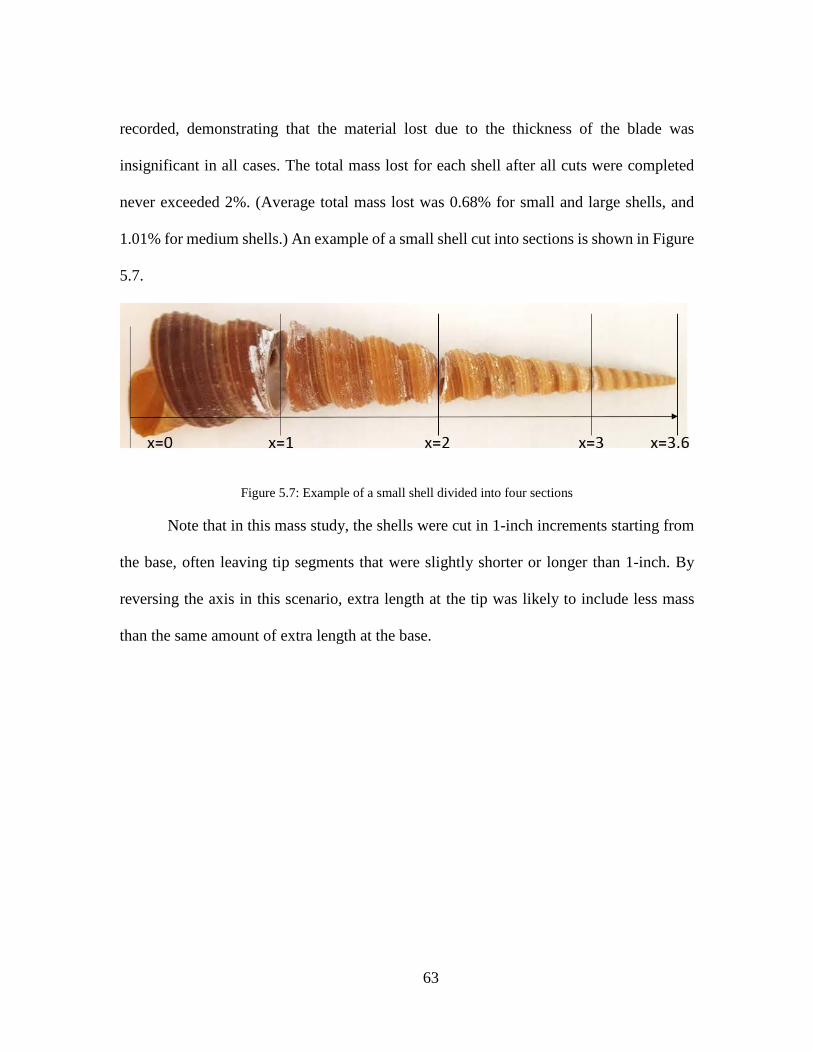
63

recorded, demonstrating that the material lost due to the thickness of the blade was

insignificant in all cases. The total mass lost for each shell after all cuts were completed

never exceeded 2%. (Average total mass lost was 0.68% for small and large shells, and

1.01% for medium shells.) An example of a small shell cut into sections is shown in Figure

5.7.

Figure 5.7: Example of a small shell divided into four sections

Note that in this mass study, the shells were cut in 1-inch increments starting from

the base, often leaving tip segments that were slightly shorter or longer than 1-inch. By

reversing the axis in this scenario, extra length at the tip was likely to include less mass

than the same amount of extra length at the base.

64

Figure 5.8: Cumulative mass as the shell grows for all shell sizes

By adding the mass of each section, we are able to determine the accumulation of

mass as the snail adds material and grows in length. Figure 5.8 shows the power law

relationship of cumulative mass as a function of theoretical “total length” at a given age,

for all shell sizes. The difference in power laws for the shell sizes supports the discussion

in Section 5.1.2 that size and age are distinct classifications. Cutting open the shells led to

the discovery of small deposits of unrecognizable material sometimes found on the internal

surface of the shell. These may be unremoved pieces of the snail or ocean debris trapped

in the shell during growth. Due to the spiraling geometry of the shell, the removal of these

substances was inconsistent and may affect the recorded mass, though it is believably less

than 10% of a shell’s total mass—a gut figure based on the visible amount.

Large shells:y = 0.7644x2.1651

R² = 0.9992

Medium shells:y = 0.5001x2.3163

R² = 0.9993

Small shells:y = 0.4955x2.2426

R² = 0.9993

0

5

10

15

20

25

30

0 1 2 3 4 5 6

CUM

ULA

TIVE

MAS

S (G

)

DISTANCE FROM TIP (INCHES)

CUMULATIVE MASS VS. TOTAL LENGTHLarge Medium Small

65

5.1.4 Density

A simple study was conducted to determine whether the density of the shell changes

as the shell grows (i.e., as a function of length). If density were determined to not be

constant throughout the material, this would complicate our understanding of shell growth.

For example, in the projections of cumulative mass in Section 5.1.3, a changing density

would suggest that growth cannot be adequately captured by shell geometry. In other

words, this would suggest any measurement at a given length may not be representative of

the actual conditions of the shell at that age. A changing density would be a significant

factor for determining mechanical strength, as density is often correlated with, and used as

a surrogate for, the strength of brittle materials (M. B. Cortie, McBean, and Elcombe 2006).

To study density as a function of length, a collection of small, medium, and large

shells were cut along their length at regular intervals—similarly to the process described

for measuring cumulative mass. However, density here is calculated as the ratio of mass

over material volume, in which volume is measured in mL as the amount of water displaced

in a graduated cylinder. Since the size of each segment was limited to approximately 1-

inch for safety reasons (i.e., finger distance from the saw blade), the air trapped inside the

segments was a concern for volume misrepresentation. (Ideally, each whorl could be

measured individually to ensure an escape path for air. Instead, a 1-inch segment near the

tip could contain as many as 15 whorls.)

To release the trapped air, a hammer and mallet were used to shatter the segments

into small fragments. For a large enough volume displacement to be significant, all of the

same segments of a single shell size were crushed and combined for a single data point.

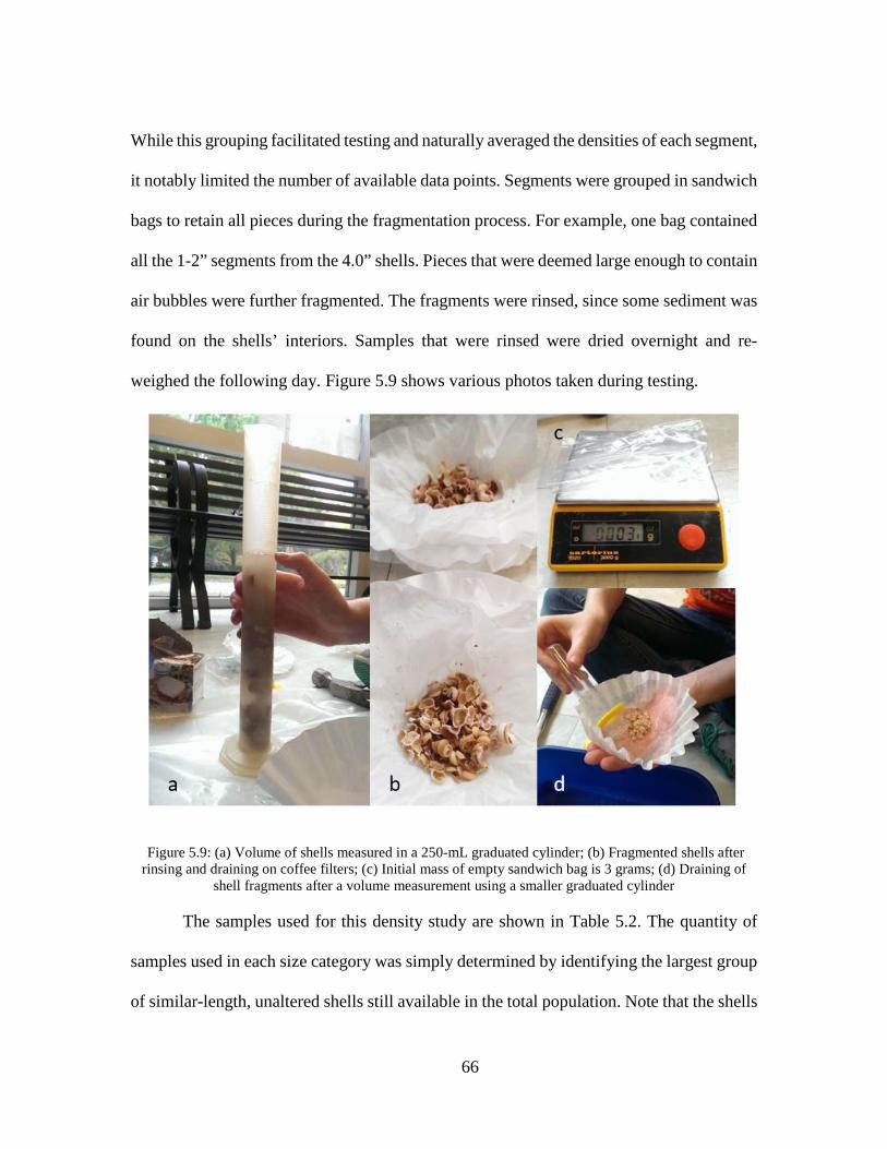
66

While this grouping facilitated testing and naturally averaged the densities of each segment,

it notably limited the number of available data points. Segments were grouped in sandwich

bags to retain all pieces during the fragmentation process. For example, one bag contained

all the 1-2” segments from the 4.0” shells. Pieces that were deemed large enough to contain

air bubbles were further fragmented. The fragments were rinsed, since some sediment was

found on the shells’ interiors. Samples that were rinsed were dried overnight and re-

weighed the following day. Figure 5.9 shows various photos taken during testing.

Figure 5.9: (a) Volume of shells measured in a 250-mL graduated cylinder; (b) Fragmented shells after rinsing and draining on coffee filters; (c) Initial mass of empty sandwich bag is 3 grams; (d) Draining of

shell fragments after a volume measurement using a smaller graduated cylinder

The samples used for this density study are shown in Table 5.2. The quantity of

samples used in each size category was simply determined by identifying the largest group

of similar-length, unaltered shells still available in the total population. Note that the shells

67

used are all very close to the minimum requirement for their size category; this helped to

minimize the amount of unusable material generated by a longer-than-intended end

segment. In these cases, a section that would ideally be divided into one full and one partial

segment could not be cut due to safety allowances. Consequently, the segments longer than

1-inch were not included due to the difficulty in accurately characterizing the extra length.

Table 5.3 shows how two segments were left out of the small category due to some

difficulty in dividing them into usable smaller sections. The data were normalized by the

number of segments used for each measurement.

Note that in this density study, the 1-inch increments were measured from the tip,

which resulted in excess length on the base-end. This axis is reversed from the mass study

described above. The excess length on the base-end logically results in much more material

that is unaccounted for, in comparison to a segment of the same length at the tip.

Table 5.2: Collection of shells used for density study

Shell size Total lengths of shells used Number of samples Small 3.3125” and 3.375” 10-12 Medium 4.0” and 4.0625” 13 Large 5.0 and 5.063” 10

Table 5.3: Diagram of which segments of small shells were used in the density study

3.3125” 3.375” Shell # 1 2 3 4 5 6 7 8 9 10 11 12 Segment 1 x x x x x x x x x x x x Segment 2 x x x x x x x x x x Segment 3 x x x x x x x x x x

Due to the grouping of segments, the density measurements unfortunately leave

only a few points from which to infer results. Future studies could increase the number of

68

sizing categories (e.g., 4.25” shells, 4.50” shells), while keeping in mind that these cut and

fragmented samples are thereby rendered unusable for other studies.

Figure 5.10: Mass of each shell segment (noncumulative) as distance from tip increases

As Figure 5.10 demonstrates, mass increases with age (i.e., as a function of distance

from the tip) in all shell sizes, as expected. Whorls closer to the tip are much smaller in

both height and width than those at the base, and require more material to generate. There

is no obvious difference between the masses of the differently sized shells in each segment.

0.001.002.003.004.005.006.007.008.009.00

10.00

0 1 2 3 4 5 6

NO

RMAL

IZED

MAS

S (G

)

SECTION # (DISTANCE FROM TIP IN INCHES)

MASS VS. HEIGHT3-inch 4-inch 5-inch

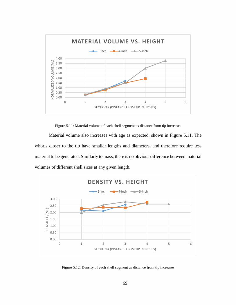
69

Figure 5.11: Material volume of each shell segment as distance from tip increases

Material volume also increases with age as expected, shown in Figure 5.11. The

whorls closer to the tip have smaller lengths and diameters, and therefore require less

material to be generated. Similarly to mass, there is no obvious difference between material

volumes of different shell sizes at any given length.

Figure 5.12: Density of each shell segment as distance from tip increases

0.000.501.001.502.002.503.003.504.00

0 1 2 3 4 5 6

NO

RMAL

IZED

VO

LUM

E (M

L)

SECTION # (DISTANCE FROM TIP IN INCHES)

MATERIAL VOLUME VS. HEIGHT3-inch 4-inch 5-inch

0.00

0.50

1.00

1.50

2.00

2.50

3.00

0 1 2 3 4 5 6

DEN

SITY

G/(

ML)

SECTION # (DISTANCE FROM TIP IN INCHES)

DENSITY VS. HEIGHT3-inch 4-inch 5-inch

70

Figure 5.12 shows the density of each segment through time and across shell sizes.

Density is found by dividing the mass in each segment by the volume of that segment.

Table 5.4 below details the averaged values of each segment.

Table 5.4: Density (g/mL) of shell segments

Section 3-inch 4-inch 5-inch Average 1 2.18 2.29 2.00 2.16 2 2.12 2.40 2.56 2.36 3 2.59 2.36 2.80 2.58 4 -- 2.76 2.63 2.70 5 -- -- 2.63 2.63 Average 2.30 2.45 2.52

As more easily observable in Table 5.4 than in Figure 5.12, there does seem to be

a slight increase in average density as shell size increases, as well as with increases in age,

but significant results are not drawn here from the few data points collected. Moreover,

these values are low in comparison to the densities of calcium carbonate—2.71 g/cm3 for

calcite and 2.93 g/cm3 for aragonite (M. B. Cortie, McBean, and Elcombe 2006).

Nacre, the most commonly referenced shell material, uses a combination of calcite

(to prevent penetration) and aragonite (to dissipate mechanical energy) (Luz and Mano

2009), in a brick-and-mortar structure that is highly composed of aragonite (Jackson,

Vincent, and Turner 1988). However, it is unclear what the composition of the T. terebra’s

calcium carbonate is, though likely not nacreous since its internal surface does not have

the iridescent characteristic of nacre. Either way, the densities found in this simple

experiment are low for what is expected of seashells.

From the available data, we do not confidently claim that density changes as a

function of size or age. However, while this basic information is sufficient for our purposes

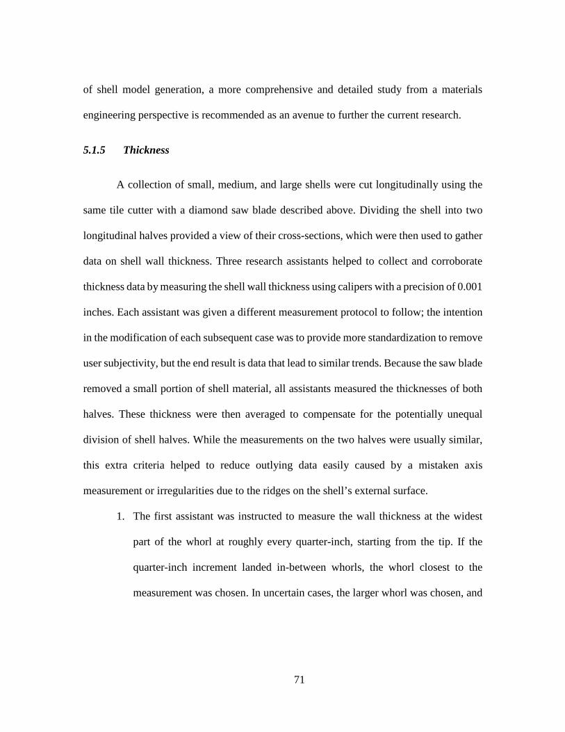
71

of shell model generation, a more comprehensive and detailed study from a materials

engineering perspective is recommended as an avenue to further the current research.

5.1.5 Thickness

A collection of small, medium, and large shells were cut longitudinally using the

same tile cutter with a diamond saw blade described above. Dividing the shell into two

longitudinal halves provided a view of their cross-sections, which were then used to gather

data on shell wall thickness. Three research assistants helped to collect and corroborate

thickness data by measuring the shell wall thickness using calipers with a precision of 0.001

inches. Each assistant was given a different measurement protocol to follow; the intention

in the modification of each subsequent case was to provide more standardization to remove

user subjectivity, but the end result is data that lead to similar trends. Because the saw blade

removed a small portion of shell material, all assistants measured the thicknesses of both

halves. These thickness were then averaged to compensate for the potentially unequal

division of shell halves. While the measurements on the two halves were usually similar,

this extra criteria helped to reduce outlying data easily caused by a mistaken axis

measurement or irregularities due to the ridges on the shell’s external surface.

1. The first assistant was instructed to measure the wall thickness at the widest

part of the whorl at roughly every quarter-inch, starting from the tip. If the

quarter-inch increment landed in-between whorls, the whorl closest to the

measurement was chosen. In uncertain cases, the larger whorl was chosen, and

72

the widest part of that larger whorl was used as the measurement point.

Measurements were taken using analog calipers with 0.001” precision.

2. The second assistant was provided the same instructions as the first assistant,

but likely rounded up to the larger whorl more frequently when quarter-inch

markings fell between whorls. This assistant took measurements of only a

subset from the shell group dedicated to thickness studies. Measurements were

taken using analog calipers with 0.001” precision.

3. The third assistant was instructed to measure the wall thickness at three points

within every whorl, starting from a diameter of 1/8” to account for many shells

that have broken tips. The three points were determined by roughly dividing

each whorl’s circumference into quarters (see Figure 5.13). Measurements were

recorded for 2 shells of each size category. This assistant used computer

graphics software ImageJ to digitally measure wall thicknesses on cross-

sectional scans of the shells.

Figure 5.13: Diagram describing Assistant #3’s measurement protocol on a cross-sectional scan

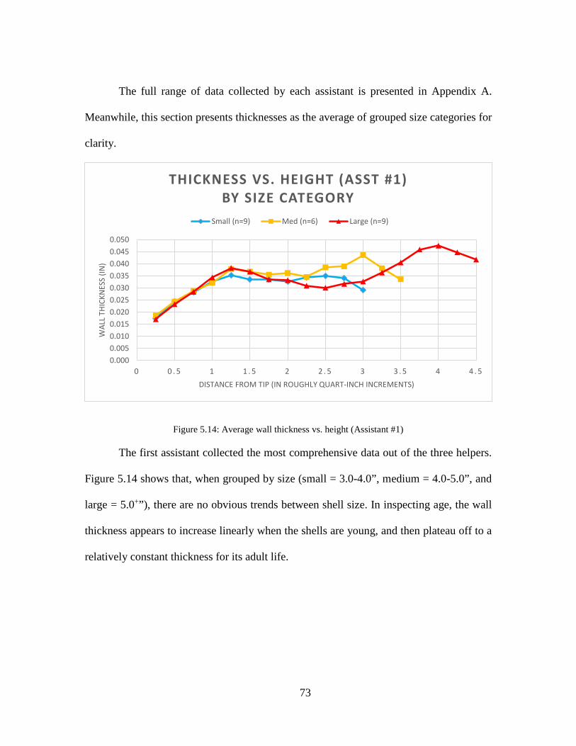
73

The full range of data collected by each assistant is presented in Appendix A.

Meanwhile, this section presents thicknesses as the average of grouped size categories for

clarity.

Figure 5.14: Average wall thickness vs. height (Assistant #1)

The first assistant collected the most comprehensive data out of the three helpers.

Figure 5.14 shows that, when grouped by size (small = 3.0-4.0”, medium = 4.0-5.0”, and

large = 5.0+”), there are no obvious trends between shell size. In inspecting age, the wall

thickness appears to increase linearly when the shells are young, and then plateau off to a

relatively constant thickness for its adult life.

0.0000.0050.0100.0150.0200.0250.0300.0350.0400.0450.050

0 0 . 5 1 1 . 5 2 2 . 5 3 3 . 5 4 4 . 5

WAL

L TH

ICKN

ESS

(IN)

DISTANCE FROM TIP (IN ROUGHLY QUART-INCH INCREMENTS)

THICKNESS VS. HEIGHT (ASST #1)BY SIZE CATEGORY

Small (n=9) Med (n=6) Large (n=9)

74

Figure 5.15: Average wall thickness vs. height (Assistant #2)

Figure 5.15 shows the thickness data collected by the second assistant. Note the

smaller quantity of sample sizes per category. While trends between shell sizes are not

obvious, the same conclusions as above can be generalized—wall thickness increase during

growth while young, with relatively constant thickness during adult years. We are limited

to these very broad generalizations, as the thickness data is rather inconsistent between

assistants and varies drastically between shells of the same size. For example, Figure 5.16

below shows the thickness data from Assistant #1 that reflect only the shells used by

Assistant #2.

0.0000.0050.0100.0150.0200.0250.0300.0350.0400.0450.050

0 0 . 5 1 1 . 5 2 2 . 5 3 3 . 5 4 4 . 5 5

WAL

L TH

ICKN

ESS

(IN)

DISTANCE FROM TIP (IN ROUGHLY QUARTER-INCH INCREMENTS)

THICKNESS VS. HEIGHT (ASST #2)3.25 avg (n=3) 3.5 avg (n=3) 4.25 avg (n=2) 5.5 avg (n=2)

75

Figure 5.16: Subset of thicknesses from Assistant #1 for comparison to Assistant #2

Note the identical sample sizes, and that the line colors are adjusted in Figure 5.16

from Figure 5.14 for easy comparison to Figure 5.15. Even though the same 10 shell

specimens are used and both assistants were given the same instructions, the measurements

vary rather drastically. Figure 5.17 shows the difference in their measurements, as a percent

over their average—measurements for the same data point can vary up to almost 60%.

0.010

0.015

0.020

0.025

0.030

0.035

0.040

0.045

0.050

0.055

0 0 . 5 1 1 . 5 2 2 . 5 3 3 . 5 4 4 . 5 5

WAL

L TH

ICKN

ESS

(IN)

DISTANCE FROM TIP (IN ROUGHLY QUARTER-INCH INCREMENTS)

THICKNESS VS. HEIGHT (ASST #1)3.25-avg (n=3) 3.5-avg (n=3) 4.25-avg (n=2) 5.5-avg (n=2)

76

Figure 5.17: Percent differences in the thickness measurements taken by assistants

Due to the inconsistencies between the first two assistants, a third assistant was

asked to repeat a subset of measurements, using only 6 samples—2 shells of each size.

Assistant #3 was instructed to use ImageJ to measure thicknesses on previously scanned

cross-sections (copies provided in Appendix B). These scans ensure preservation of the

shell image, and repeated measurements are likely more consistent than measurement by

analog calipers. ImageJ is an open source image processing software developed by the NIH

and freely available for download. There are a few relationships we can investigate from

Assistant #3’s work, which uses whorl number, rather than distance:

1. Effect of measurement location within a whorl;

2. How thickness varies by shell size; and

3. Relationship of whorl number to distance from the tip.

0%

10%

20%

30%

40%

50%

60%

70%

0 1 2 3 4 5

% D

IFFE

REN

CE IN

THI

CKN

ESS

DISTANCE FROM TIP (IN ROUGHLY QUARTER-INCH INCREMENTS)

% DIFFERENCE IN THICKNESS BETWEEN ASSISTANTS VS. HEIGHT

3.5-avg 3.5-avg 4.25-avg 5.5-avg

77

5.1.5.1 Effect of Measurement Location within a Whorl

Figure 5.18: Effect of measurement location within a whorl on wall thickness

Figure 5.18 shows the shells aggregated by size, but similar trends are

observed across all shell sizes. The trends in the figure suggests that the quarter-whorl

marking nearest to the base is typically the thickest of the three measurements within a

whorl. However, at the largest whorls, the tip measurement often exceeds the thicknesses

of the other two points. This perhaps captures the progress of the addition of material,

where a new whorl is necessarily first attached to the previous whorl (nearer to the tip)—

the other quarter-whorl measurements may simply have not had time to “catch up”.

5.1.5.2 Note on Aperture Thickness

Observations of the shell samples show evidence of material layering, as the lip of

the aperture often has a thinner wall than the rest of the shell. Photos of base whorls from

0

0.01

0.02

0.03

0.04

0.05

1 3 5 7 9 11 13

WAL

L TH

ICKN

ESS

(IN)

WHORL NUMBER AFTER 1/8" MARKING

THICKNESS VS. WHORL NUMBERFOR WHORL MEASUREMENT LOCATION

Tips Centers Bases

78

select shells that demonstrate this layering effect are shown in Figure 5.19. The decreasing

thickness as it approaches the leading edge may have to do with the way the mollusk

deposits material from its mantle, as discussed in its ecological background (Section 4.1.1)

The thickness of the aperture is inconsistent between even shells of similar sizes. Future

studies may investigate whether the thickness of this last section is a correlate to shell age,

suggesting that perhaps the mollusk has reached full maturity when the aperture follows

the same thickness trend as the rest of the shell.

Figure 5.19: Photos of layering in select base shells (left) and illustration of aperture cross-section (right)

79

5.1.5.3 Thickness vs. Shell Size (as Measured by Assistant #3)

Figure 5.20: Thicknesses of different shell sizes, using the average of the three quarter-whorl markings

Using the average thickness of each whorl (averaging tip, center, and base

measurements), we can investigate the differences in shell size, as shown in Figure 5.20. It

does not appear that shell size has an effect on the thickness of the shell wall.

0

0.01

0.02

0.03

0.04

0.05

0.06

0.07

0 2 4 6 8 1 0 1 2 1 4 1 6

WAL

L TH

ICKN

ESS

(IN)

WHORL NUMBER AFTER 1/8" MARKING

THICKNESS VS. WHORL NUMBERFOR SHELL SIZES

Avg of smalls Avg of mediums Avg of larges

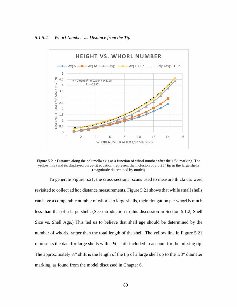
80

5.1.5.4 Whorl Number vs. Distance from the Tip

Figure 5.21: Distance along the columella axis as a function of whorl number after the 1/8” marking. The yellow line (and its displayed curve-fit equation) represent the inclusion of a 0.25” tip in the large shells

(magnitude determined by model)

To generate Figure 5.21, the cross-sectional scans used to measure thickness were

revisited to collect ad hoc distance measurements. Figure 5.21 shows that while small shells

can have a comparable number of whorls to large shells, their elongation per whorl is much

less than that of a large shell. (See introduction to this discussion in Section 5.1.2, Shell

Size vs. Shell Age.) This led us to believe that shell age should be determined by the

number of whorls, rather than the total length of the shell. The yellow line in Figure 5.21

represents the data for large shells with a ¼” shift included to account for the missing tip.

The approximately ¼” shift is the length of the tip of a large shell up to the 1/8” diameter

marking, as found from the model discussed in Chapter 6.

y = 0.0196x2 - 0.0224x + 0.4125R² = 0.997

0

0.5

1

1.5

2

2.5

3

3.5

4

4.5

5

0 2 4 6 8 1 0 1 2 1 4 1 6

DIST

ANCE

FRO

M 1

/8" M

ARKI

NG

(IN)

WHORL NUMBER AFTER 1/8" MARKING

HEIGHT VS. WHORL NUMBERAvg S Avg M Avg L Avg L + Tip Poly. (Avg L + Tip)

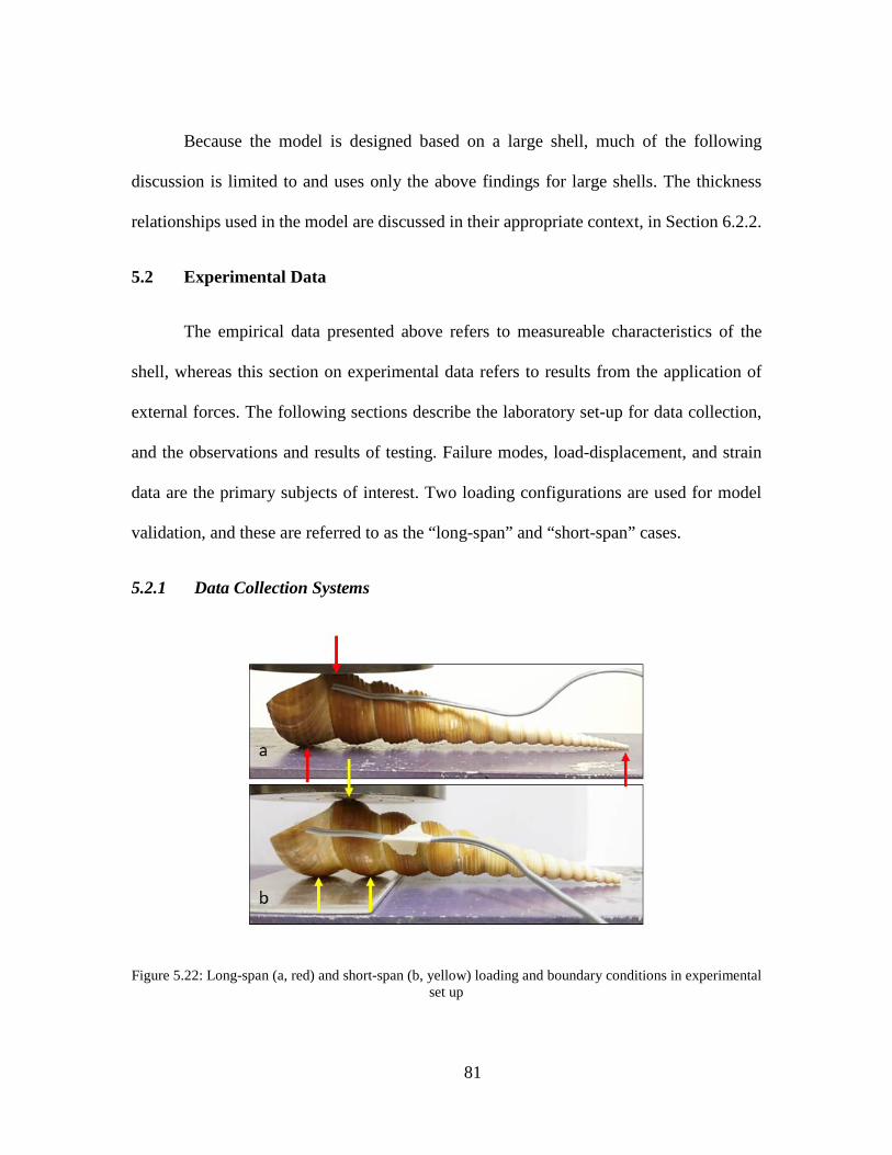
81

Because the model is designed based on a large shell, much of the following

discussion is limited to and uses only the above findings for large shells. The thickness

relationships used in the model are discussed in their appropriate context, in Section 6.2.2.

5.2 Experimental Data

The empirical data presented above refers to measureable characteristics of the

shell, whereas this section on experimental data refers to results from the application of

external forces. The following sections describe the laboratory set-up for data collection,

and the observations and results of testing. Failure modes, load-displacement, and strain

data are the primary subjects of interest. Two loading configurations are used for model

validation, and these are referred to as the “long-span” and “short-span” cases.

5.2.1 Data Collection Systems

Figure 5.22: Long-span (a, red) and short-span (b, yellow) loading and boundary conditions in experimental set up

82

Shell specimens were placed in a Universal Testing Machine (UTM) to be loaded

laterally in a three-point loading condition (Figure 5.22). The UTM is displacement-driven,

meaning the system input is a displacement rate and a direction, which consequently

increases the load on the specimen as the space between the loading heads decreases. The

UTM has a load cell, produced by Thames Side-Maywood (Series U4000) with a load

capacity of 50 kN. In cases where other sensors were attached to the shell, a second load

cell was placed below the shell; the two systems could then be synced by the readings of

each load cell. This second load cell is produced by Omegadyne (model LC412-1K) and

has a load capacity of 1K lbs. Figure 5.23 shows the long-span set up of a shell in the UTM,

sandwiched by two load cells, and with a strain gage attached. The data from the

Omegadyne load cell and strain gages (both sensors external of the UTM) were recorded,

processed, and synced through a National Instruments Data Acquisition System (DAQ).

83

Figure 5.23: Test set-up in UTM with two load cells

In addition to the UTM and two load cells, strain gages were placed on some

specimens to observe changes in strain as the shell was loaded. The placement of the strain

gages in the long-span configuration is shown in Figure 5.24. The strain gages are FLA-1-

11-1L gages produced by Texas Instruments, with a gage length-by-width of 1x1.3 mm,

and a backing length-by-width of 3x2.0 mm. The placement of gages was slightly

inconsistent due to difficulties caused by its small size, but the goal location was just inside

the aperture on the surface roughly perpendicular to the loading direction. This location

was initially selected for its smooth and relatively flat surface and external accessibility.

84

Figure 5.24: Placement of strain gages in the long-span configuration

5.2.2 Shell Orientation and Boundary Conditions

As shown in Figure 5.23, the shell is oriented “aperture-up” such that the UTM

loading plate contacts the whorl previous to the aperture, aligning it with the axis of

loading. The aperture lip is rotated to be as close to the descending loading plate as possible,

without exceeding the previous whorl in absolute height. There is some compromise

involved to identify a stable spot that does not induce rolling.

The placement of the aperture is important since the last whorl in many of the shells

decreases in thickness as it approaches the aperture lip (see Section 5.1.5.2). By rotating

the lip to be as close to the loading plate as possible, we ensure that the thickest possible

portion of the last whorl acts as the support. Figure 5.25 shows an early test where the shell

was placed “aperture-down”, causing the base to crush first. The crushing of the base

eliminated a stable support, causing the shell tip to slowly rotate away from the table as the

load was increased.

85

Figure 5.25: Incorrect “aperture-down” configuration leads to base crushing and tip rotating upward

5.2.2.1 Long-Span Configuration

It is significant to note that the shell acts similarly to a simply supported beam in

the long-span configuration, as it is only supported at the tip and at the base—the shell may

grow less linearly than we are able to capture after all. The shell can be seen sitting on the

two support points in Figure 5.22. The long-span configuration is approximated as three

point-loads—two as supports and one at the loading point—since the shell’s ridge

protrusions bear the brunt of the load. The shells ridges are clearly observable in Figure

5.25.

5.2.2.2 Short-Span Configuration

The short-span configuration used all the same instrumentation as the long-span

configuration, with only a change in the location of the supports and the placement of the

strain gage. By placing a second steel plate under the shell under only the last two base

whorls, the shell is effectively elevated and balanced on two new support points. Figure

5.22 shows this configuration with the UTM crosshead descended to its maximum load.

Note that the tip (which was previously broken) is not touching any surface.

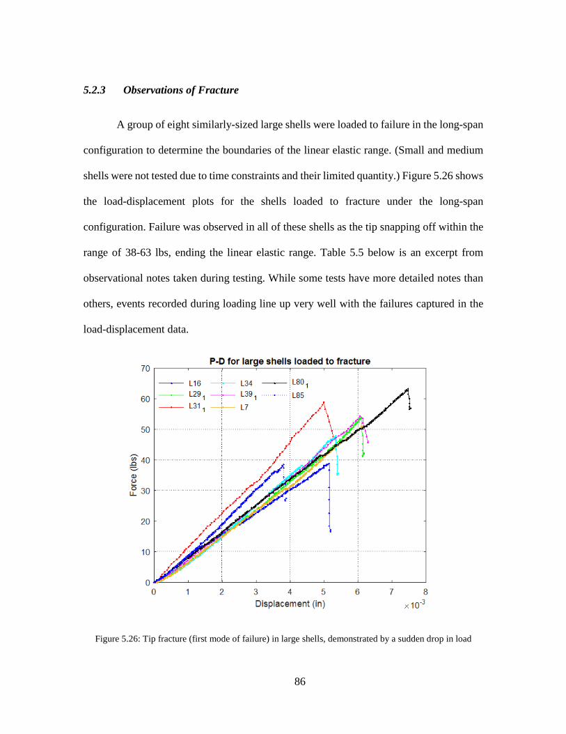
86

5.2.3 Observations of Fracture

A group of eight similarly-sized large shells were loaded to failure in the long-span

configuration to determine the boundaries of the linear elastic range. (Small and medium

shells were not tested due to time constraints and their limited quantity.) Figure 5.26 shows

the load-displacement plots for the shells loaded to fracture under the long-span

configuration. Failure was observed in all of these shells as the tip snapping off within the

range of 38-63 lbs, ending the linear elastic range. Table 5.5 below is an excerpt from

observational notes taken during testing. While some tests have more detailed notes than

others, events recorded during loading line up very well with the failures captured in the

load-displacement data.

Figure 5.26: Tip fracture (first mode of failure) in large shells, demonstrated by a sudden drop in load

87

Table 5.5: Excerpt from testing notes lines up closely with cracks determined in P-D data. The number afer the dash refers to the test number for that shell specimen.

Shells loaded to fracture

Testing notes Important events from P-D plots

L7-1 Clean break (with minor local failure at base), tip broke off easily when touched

Slope change at 50 lbs

L16-1 1/2" Tip broke off @ -38.6 lbs, continue to load, another 3/4" piece tip broke off; test ended at 132 lbs

Crack at 39 lbs Second crack at 132 lbs

L29-1 Tip broke off @ ~40-50, whorl broke off at 115 lbs, minimal crushing at base

Crack at 53 lbs Larger crack at 115 lbs

L31-1 5.125x1.125 slightly smaller since ran out of shells +/- 1/16"

Crack at 59 lbs Larger crack at max load of 112 lbs

L34-1 Slightly larger than rest in set (base diameter: 1.188 in.) Speculation is tip broke off, but nothing is observable other than loud crack. Tip comes off when handled after 2nd test

Cracks at 48 lbs, 114 lbs, 119 lbs

L39-1 First crack 55-65 lbs, max load @ 112 Crack at 54 lbs Larger crack at 112 lbs

L80-1 Tip broke at 67.3 (change in shell loading pt), noticed rotation around 190 lbs, wavered for a long time, whorl finally slowly fell off around 155 lbs, crushed at base

Crack at 63 lbs

L85-1 Tip broke off Crack at 39 lbs, 110 lbs, 118 lbs

In many tests, the shells were continually loaded until the second mode of failure

occurred—typically observed as the base whorl fracturing at its suture to the previous

whorl. While this failure mode was consistent by observation, it is not investigated or

validated in the subsequent linear elastic study. In addition to being outside the linear

elastic capacity of the model, the boundary conditions of the long-span configuration

change once the tip has broken—the span length shortens and the shell’s angle changes

slightly as it finds a new whorl to support itself.

Many of the fractured shells shown in the data of Figure 5.26 are pictured in Figure

5.27 below, which illustrates the two consistent modes of failure—tip snapping and then

base crushing. There are two shells in Figure 5.27 that are not included in the fracture data

88

above due to their uniqueness: L92 (third from the left) and L22 (second from the right).

L92 has an abnormal, circular hole in the middle of its spire, which resulted in nonlinear

load-displacement data. This physical irregularity was not observed in any of the other 202

samples, and so this data was discarded. The hole is likely caused by a type of borer, which

is known to be a predator of tower-like mollusks (M. Cortie 1989). Notice that L22’s

broken tip is much smaller than the others in the photo. Moreover, note the differences in

geometry of L22 from the other shells—while it ranked only 36th in height and 41st in

diameter out of 84 large shells, it had a mass within the top 11 of all 202 shells. Shell L16

interestingly failed twice at the tip before crushing at the base.

Figure 5.27: Shells L16, L29, L92, L80, L39, L22, and L31 (left to right) after fracture

5.2.4 Load-Displacement Data

The common data collected by both load cells are time duration of the test and the

magnitude of the applied load. While most of this study uses load-displacement as the

standard, the syncing between systems is necessarily done through the time (in seconds).

The “start” time for the two systems may be different, but they are easily synced by

89

“events” in the data, such as changes in load. A basic description of the data processing

and the code developed to sync the data from the UTM and DAQ is provided in Appendix

C.

Figure 5.28: Comparison of UTM and DAQ load data in a linear elastic test loaded up to 30 lbs (top); and

corresponding load-displacement plot (bottom)

90

Figure 5.28 is a very typical representation of all linear elastic tests conducted. The

force data from the two different systems align fairly well, and the difference between the

two systems never exceeds 1 lb. A range of 0-30 lbs was chosen for linear testing to avoid

damaging the specimens that have strain gages installed. A lower end of approximately 35

lbs was determined to be the failure load for shells of similar size. Figure 5.28 (top)

demonstrates agreeable precision in the syncing between systems, and therefore instills

confidence in the accuracy of the load-displacement data collected by the UTM system

(Figure 5.28, bottom).

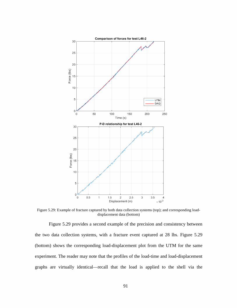
91

Figure 5.29: Example of fracture captured by both data collection systems (top); and corresponding load-

displacement data (bottom)

Figure 5.29 provides a second example of the precision and consistency between

the two data collection systems, with a fracture event captured at 28 lbs. Figure 5.29

(bottom) shows the corresponding load-displacement plot from the UTM for the same

experiment. The reader may note that the profiles of the load-time and load-displacement

graphs are virtually identical—recall that the load is applied to the shell via the

92

displacement-driven UTM at a predetermined, constant rate (usually 0.001 in/min), so the

displacement is directly related to time. Except in cases where the loading is paused and

restarted, the profiles of the two plots are effectively identical.

Figure 5.30: Load-displacement data from all linear elastic tests

By Hooke’s law (𝐹𝐹 = 𝑘𝑘𝑥𝑥), the slope of the load-displacement graph represents the

global stiffness of each shell. Figure 5.30 shows the range of stiffnesses collected during

linear elastic testing of the long-span configuration. This range is used as the limits of

allowable stiffnesses in model validation. Note that many of the eligible shells were tested

repeatedly (up to 10 times) in the linear elastic range, as long as they demonstrated no signs

of plasticity. Repeated tests are included as individual lines in Figure 5.30. A larger figure

with its 53 data labels is provided in Appendix A.

93

5.2.5 Load-Strain Data

Figure 5.31: Load-strain data from eligible long-span tests

Figure 5.31 depicts the strain data collected from shells in the long-span

configuration. The smaller quantity of tests presented here is due to the elimination of some

shells in cases where the strain gage’s faulty installation was presumed to be the cause of

peculiar trends (e.g., too much epoxy, epoxy inadvertently spread onto the electrical

surface of the gage, damage to wiring, etc.).

As Figure 5.31 shows, the strain data is relatively difficult to interpret, partially due

to the naturally grainy output of strain gages, and partially due to the very small magnitudes

of strains collected. Note that the curvy lines are the result after data processing, which

included a 9th order Butterworth low-pass filter. (Processing details are included in

94

Appendix C.) While the curvy lines are not ideal, they are easier to interpret than the raw

data, an example of which is provided in Figure 5.32.

Figure 5.32: Example of raw strain data typical of all data collected

While this messy strain data has very limited usefulness, we are able to see a general

increase in strain as the load increases. Recall that in the long-span configuration, the gage

was placed approximately perpendicular to the axis of loading, so this direct relationship

is expected. However, the maximum magnitude of strain captured in this orientation is less

than 20 microstrain—an extremely low number for typical engineering applications and

general strain gage data. The finite element model corroborates a “low value” but is unable

to confirm values as small as 20 microstrain in the gage area. Figure 5.33 shows the vector

plot of the gage area, which has insignificant values in all directions. For these reasons, the

collected strain data are not used for model validation as intended.

95

Figure 5.33: Vector plot of principal strains in the long-span shell with approximate gage placement shown

5.2.6 Notes on Short-Span Data

Figure 5.34: Load-displacement data from the same shell in short-span configuration

020406080

100120140160180

0 0.001 0.002 0.003 0.004 0.005 0.006 0.007 0.008 0.009 0.01

LOAD

(LBS

)

DISPLACEMENT (INCHES)

P-D DATA FOR SHORT-SPANTrial 1 Trial 2

96

The short-span shell was loaded up to 170 lbs in experimental testing and generally

remained in the linear elastic range (Figure 5.34). The load data did not indicate any

fractures and no obvious failures were observed by eye. However, the tests were stopped

when small cracking sounds were heard around 175 lbs, and the shell was removed from

the UTM. Some local crushing at the loading point was observed on the shell surface, as

shown in Figure 5.35. This curious phenomenon of visible damage but no evidence of

fracture in the data is discussed later in Section 6.3.4.2. This new loading configuration is

capable of supporting larger loads, has a different failure mode than the long-span

configuration, and may be more representative of the compressive forces due to a predator.

Future studies may consider a more holistic approach towards simulating the loads a shell

experiences in its natural habitat (e.g., aperture orientation, different types of predators).

Figure 5.35: Local crushing in short-span shell at maximum load of 175 lbs

97

Figure 5.36: Simulated 3rd principal strain in (top) long-span model and (bottom) short-span model

98

Model simulations predicted strain magnitudes as large as 400 microstrain in

compression on the internal lip of the aperture in the long-span setup (Figure 5.36, top),

and up to 1000 microstrain in the short-span configuration (Figure 5.36, bottom). However,

new gages were added to this location in short-span testing to no avail. Figure 5.37 shows

the strain data (recorded manually due to technical difficulties) for four linear elastic tests

on one shell. The wide discrepancies in strain data are discouraging, and ultimately strain

data are not used due to low precision. Future researchers are encouraged to either use shell

species that are larger at maturity, or have professional help from a technician for installing

small instrumentation.

Figure 5.37: Load-strain data in the short-span configuration for four tests repeated on the same shell

0

20

40

60

80

100

120

140

0 5 1 0 1 5 2 0 2 5 3 0 3 5

FORC

E (L

BS)

MICROSTRAIN

LOAD-ST RAI N I N SHORT -SPAN CONFI GURATI ON

L61_1 L61_2 L61_3 L61_4

99

CHAPTER SIX

BUILDING THE MODEL

The model building process can be divided into two main sections: the generation

of a geometry, and the analysis in finite element software. The shape of the shell is defined

by a set of input parameters, such as specific angles, profiles, and number of revolutions.

A series of mathematical equations that characterize these geometric properties are

implemented to build each sample in MATLAB software. The program culminates in the

export of a series of nodes and elements, which are input into ANSYS finite element (FE)

software in the second phase of modeling. Material properties and boundary conditions are

then added in ANSYS to create a structural model of the shell. This chapter describes

technical details of the geometric generation and development of the FE model.

6.1 MATLAB Geometry Generation

First and foremost, this project is heavily founded on the MATLAB model that Dr.

Hamed Rajabi of the University of Kiel (Christian-Albrechts-Universität zu Kiel)

generously shared, which acted as a starting point for this study. Improvements have been

added and modifications made for the different gastropod species. Because Rajabi’s work

is foundational for this research, the reader is directed to his papers for more technical

details (Faghih Shojaei et al. 2012; Rajabi et al. 2014), but some basic concepts are

replicated here for convenience.

As covered in Section 4.2, the history of shell modeling is long and windy, and

there are multiple approaches and simplifications that can be made in digital shell

100

generation. This project uses Rajabi’s modern technique, which follows the studies of some

historical models (e.g., Illert’s use of Frenet frames) and sidesteps others (e.g., Raup’s

earlier models) —the decisions for which to build upon are described in his papers. Rajabi’s

approach is used here due to the promising results of his simulations in addition to the

accessibility of his code as a stepping stone.

While this project focuses on a different species than in Rajabi’s work, the variables

that control shell geometry are generalized to all spiraled gastropod shells. Figure 6.1

shows an original diagram of Rajabi’s variables (with more detail than in Figure 4.5).

Minor modifications are made to these; most notably, the generating curve is customized

for a T. terebra.

Upon closer inspection, the Turritella nivea that Rajabi claims to have modeled is

categorized by the World Register of Marine Species as an Aclis minor, after a number of

historical taxonomical errors. This discrepancy in superfamily, let alone species, may

account for many differences between our models.

101

Figure 6.1: Diagram of shell variables (Faghih Shojaei et al. (2012), with permission)

Variables can be grouped by their effect on the geometry of the model: growth

constants, generating curve (G.C.) orientation, and whorl divisions. The description of

these variables are as follows:

• Growth constants:

o Alpha (𝛼𝛼) is the angle between the radius of the helicospiral and its tangent

in the x-y plane. While theoretically measurable by image processing

software, the dorsal view of the shell is difficult to capture accurately. Alpha

controls the “tightness of the coil”, and a larger alpha (with all other

102

variables held constant) results in a shorter shell with more overlap in

adjacent whorls.

o Beta (𝛽𝛽) describes the angle between the z-axis (referred to here often as

the “columella axis” for clarity) and the center of generating curve.

Increasing beta (with all else constant) increases the transverse distance

between generating curves on opposite sides of the columella. An

unreasonably large beta can even erroneously create an umbilicus in the

model. Beta can be theoretically be measured in a cross-sectional scan, but

the centroid of each generating curve is difficult to pinpoint by eye.

o Ro refers to the initial length of the helicospiral’s radius at the tip of the

shell, since realistic shells do not converge to a single point. In other words,

this is the “missing tip”, measured from the idealized tip point (with

coordinates 0, 0, 0) to the location where the physical tip begins. Ro can be

reasonably measured in a cross-sectional scan by identifying the

convergence point of the shell exterior and measuring the distance from this

hypothetical tip to the start of the shell.

• Generating curve (G.C.) constants:

o The orientation of the generating curve is determined by three variables: 𝜙𝜙,

𝜇𝜇, and 𝜔𝜔. These variables rotate the face of the generating curve in its local

axis, whose origin is at the centroid of the generating curve. These variables

are depicted in Figure 6.2. While these variables are provided in Rajabi’s

code, they are not described in his papers. The effects of their values are

103

presented in the figure below through experimental discovery and some

personal communication with Rajabi.

Figure 6.2: Generating curve (G.C.) constants and their rotational effect on G.C. orientation; The G.C. lies in the y-z plane, and the origin of the local axis lies at the centroid of the G.C.

• Whorl constants:

o The number of whorls in a shell is independent of all other variables and

can be determined by counting on a physical specimen. A whorl is a

complete revolution around the columella axis.

o Thetanum (often referred to as TN) is a variable found in Rajabi’s code that

determines the number of divisions between the initial angle of the tip and

the final angle 𝜃𝜃 at the aperture. Theta is dependent on whorl number, as

each whorl comprises 2𝑝𝑝𝑖𝑖. An increase from TN = 500 (“TN500”) to TN =

5000 (“TN5000”) is shown in Figure 6.3. Thetanum is used as the variable

for increasing mesh density.

104

Figure 6.3: TN500 (left) vs. TN5000 (right)

Table 6.1: List of input parameters used in the original code and in this model

Parameter Rajabi’s “Turritella” Current study 𝛼𝛼 (degrees) 88.6 88.63 𝛽𝛽 (degrees) 3.6 3.3 Ro (mm) 15 6.8 𝜙𝜙 (degrees) 8 𝜇𝜇 (degrees) 0 𝜔𝜔 (degrees) -2 Number of whorls 15 19.75 thetanum (TN) 500 5000

Table 6.1 shows the values used for each input parameter in Rajabi’s original

“Turritella” model and the one generated here. Note that the generating curve constants

were not altered from their original values, due to their complex effect on the global

geometry and difficulties in pinpointing their accurate range for a specific species. In this

case, we assumed Rajabi’s values were close enough to the T. terebra.

The primary parameters of interest can then be boiled down to 𝛼𝛼,𝛽𝛽, and Ro, which

are drawn from shell L83 (ID #83 of the population of large samples)—the “standard” large

shell that the model is designed for. Ultimately, height and width were the variables

controlling the final geometry, and the three primary parameters were adjusted slightly

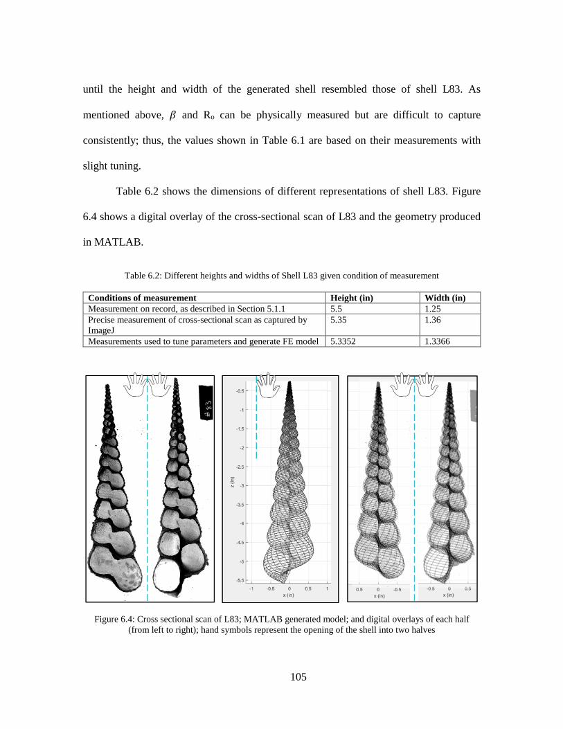
105

until the height and width of the generated shell resembled those of shell L83. As

mentioned above, 𝛽𝛽 and Ro can be physically measured but are difficult to capture

consistently; thus, the values shown in Table 6.1 are based on their measurements with

slight tuning.

Table 6.2 shows the dimensions of different representations of shell L83. Figure

6.4 shows a digital overlay of the cross-sectional scan of L83 and the geometry produced

in MATLAB.

Table 6.2: Different heights and widths of Shell L83 given condition of measurement

Conditions of measurement Height (in) Width (in) Measurement on record, as described in Section 5.1.1 5.5 1.25 Precise measurement of cross-sectional scan as captured by ImageJ

5.35 1.36

Measurements used to tune parameters and generate FE model 5.3352 1.3366

Figure 6.4: Cross sectional scan of L83; MATLAB generated model; and digital overlays of each half

(from left to right); hand symbols represent the opening of the shell into two halves

106

In addition the modifying the parameters discussed above, the shape of the

generating curve was also customized for the Turritella terebra. By extracting the G.C.

outline from the final whorl in a cross-sectional scan, this 2D shape can be used as the

template for which whorls are created from as they revolve around the columella axis. The

reader is directed to Rajabi’s papers and Jirapong and Krawczyk (2003) for details on the

theory behind the revolutions. A simple code for extracting the G.C. from a cross-sectional,

black and white image is provided in Appendix E. This code uses basic image processing

techniques on a manually isolated aperture to determine the curve-fit function. An example

of a manually extracted G.C. from L83 and its accompanying curve-fit is shown in Figure

6.5. The resulting curve-fit function is used as the shape that is rotated around the central

axis.

Figure 6.5: Manually extracted generating curve outline and curve-fit function generated from outline

107

6.1.1 Other Modifications to Code: Tying Sutures

Other major modifications to Rajabi’s code include the implementation of varying

thickness as a function of height (Rajabi used a uniform thickness through his shells); and

the tying of whorls to each other through sutures. The lack of ties between whorls is a

significant gap in Rajabi’s code that would have not been critical in his work on the smaller,

rounder Otala shell, but becomes a flaw in the Turritella when loaded under bending

stresses. Moreover, this shortcoming is unobservable in MATLAB, since the applications

of loads is required to see the unfurling of sutures.

Figure 6.6: Untied sutures under exaggerated displacement in Rajabi’s code when adapted for T. terebra

In Rajabi’s code, shell elements are created automatically when bounded by four

nodes (the element’s corners). The overlooked item involved multiple nodes existing in the

same space, rather than attaching adjacent elements to the same node. This resulted in the

shell acting like a giant spring, unfurling under load. An example of the shell “unfurling”

is shown in Figure 6.6, where the sutures are highlighted as white borders in the shell, and

the gaps between whorls (and particularly at the base) is evident. Note that the

displacements in Figure 6.6 are scaled by 900,000 and are not noticeable with true-scale

108

displacements. Appendix F provides the section of code that adapts Rajabi’s work to delete

overlapping nodes and effectively tie the whorls together.

6.2 ANSYS Finite Element Modeling

The geometry generated by the MATLAB model (e.g., Figure 6.4) can then be

imported into ANSYS finite element software through direct generation to create nodes

and shell elements. (“Direct generation” refers to the generation of a geometry through

imported files, rather than building one in the user interface. See ANSYS help documents

for more information.) This model uses SHELL181 elements, the simplest version of the

four-node shell element, with six degrees of freedom at each node. A new coordinate

system is used in ANSYS to more easily visualize the shell as sitting on a surface—the

same orientation as it is loaded in the UTM. Figure 6.7 shows the coordinate system used

in the ANSYS model. Due to an idiosyncrasy of the software, this coordinate system cannot

be displayed at the same time as other symbols.

Figure 6.7: Coordinate system used in the ANSYS model, viewing the shell in the y-z plane with x pointing out of the page

Only two material properties are needed to generate this linear, elastic, isotropic

model—Young’s Modulus and Poisson’s ratio. Both variables used in this model adopt the

109

values proposed by Rajabi, which are 50 GPa (7251887 psi) for Young’s Modulus, and a

Poisson’s ratio of 0.31. However, it should be noted that a review of literature on the

elasticity of calcium carbonate shows that 50 GPa may be on the lower end of a typical

range. (For example, M. B. Cortie, McBean, and Elcombe (2006) report 70-80 GPa,

Jackson, Vincent, and Turner (1988) report “on the order of 70 GPa”, and Davidson (2009)

reports as high as 80-120 GPa, depending on crystalline orientation.)

6.2.1 Boundary Conditions

The boundary conditions of the model simulate the setup during experimental

testing, as described in Section 5.2.1. Due to the curvature of the shell, in addition to the

ridges on the exterior surface, the boundary conditions are reasonably approximated as

point loads. The shells with their simulated boundary conditions are shown in Figure 6.8.

Table 6.3 details the constraints applied at each boundary condition.

Table 6.3: List of locations and constraints on boundary conditions

Boundary area Location Boundary condition Base support Lowest point on last whorl X,Y,Z displacement constraints Tip support Lowest point on first whorl (long-

span) or second-to-last whorl (short-span)

X,Y displacement constraints

Loading point Highest point on second-to-last whorl

X displacement constraint Applied load

110

Figure 6.8: Long-span (top) and short-span (bottom) loading and boundary conditions in simulation

While these point-load boundary constraints help to keep the model stable, future

research should consider modeling friction forces rather than use these simplifications.

However, in all simulations, the x- and z-constraints only support considerably less than

1% of the load applied in the y-direction. These low magnitudes instill confidence that the

model is primarily transferring load in the y-direction and that the constraints in the other

directions do not significantly detract from the intended simulation.

A mathematical way to view these displacement constraints as inconsequential

frictional forces is to check that their directional ratios are less than the static friction

constant, assumed to be 0.1 between the shell and the steel plate (Faghih Shojaei et al.

2012). In this model, the reaction force in the y-direction is equivalent to the normal force,

and thus, we check if

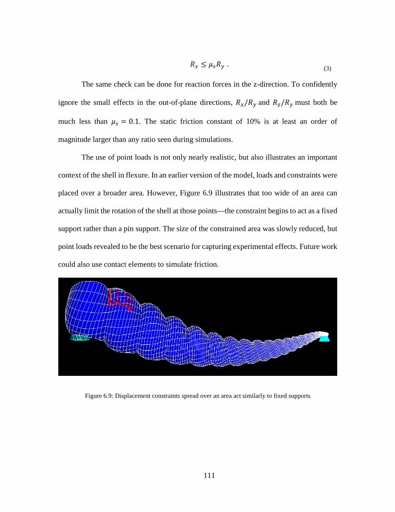
111

𝑅𝑅𝑥𝑥 ≤ 𝜇𝜇𝑠𝑠𝑅𝑅𝑦𝑦 . (3)

The same check can be done for reaction forces in the z-direction. To confidently

ignore the small effects in the out-of-plane directions, 𝑅𝑅𝑥𝑥/𝑅𝑅𝑦𝑦 and 𝑅𝑅𝑧𝑧/𝑅𝑅𝑦𝑦 must both be

much less than 𝜇𝜇𝑠𝑠 = 0.1. The static friction constant of 10% is at least an order of

magnitude larger than any ratio seen during simulations.

The use of point loads is not only nearly realistic, but also illustrates an important

context of the shell in flexure. In an earlier version of the model, loads and constraints were

placed over a broader area. However, Figure 6.9 illustrates that too wide of an area can

actually limit the rotation of the shell at those points—the constraint begins to act as a fixed

support rather than a pin support. The size of the constrained area was slowly reduced, but

point loads revealed to be the best scenario for capturing experimental effects. Future work

could also use contact elements to simulate friction.

Figure 6.9: Displacement constraints spread over an area act similarly to fixed supports

112

6.2.2 Varying Thickness

Figure 6.10: Aggregated thickness data for the two large shells measured by all assistants

Figure 6.10 shows the aggregated thickness data collected by the three research

assistants for shells L27 and L49—the two large shells that were measured by all parties.

The aggregated data reflects measurements after a shift in height to account for the different

systematic origins. A linear relationship of the wall thickness as a function of height (blue

line in Figure 6.10) was found to be

𝑚𝑚𝑚𝑚𝑚𝑚𝑚𝑚𝑚𝑚𝑚𝑚𝑚𝑚𝑑𝑑 𝑤𝑤𝑚𝑚𝑤𝑤𝑤𝑤 𝑡𝑡ℎ𝑖𝑖𝑐𝑐𝑘𝑘𝑖𝑖𝑚𝑚𝑚𝑚𝑚𝑚 = 0.0047 ∗ 𝑑𝑑𝑖𝑖𝑚𝑚𝑡𝑡𝑚𝑚𝑖𝑖𝑐𝑐𝑚𝑚 𝑓𝑓𝑚𝑚𝑜𝑜𝑚𝑚 𝑡𝑡𝑖𝑖𝑝𝑝 + 0.023. (4)

However, an empirical relationship was found during model tuning that better

simulated displacement and failure than the relationship given in Equation (4). The final

thickness equation used in the model is an average of Equation (4) and a uniform thickness

Measured thickness = 0.0047x + 0.023R² = 0.4901

0.000

0.010

0.020

0.030

0.040

0.050

0.060

0.070

0 1 2 3 4 5 6

WAL

L TH

ICKN

ESS

(IN)

DISTANCE FROM TIP (INCHES)

THICKNESS MEASUREMENTS FOR L27, L49

L27, L49 measurements Modeled thickness

Linear (L27, L49 measurements)

Modeled thickness = 0.0024x +0.029

113

of 0.034 inches (the average thickness of the averaged data from large shells). The equation

is given as

𝑚𝑚𝑜𝑜𝑑𝑑𝑚𝑚𝑤𝑤𝑚𝑚𝑑𝑑 𝑤𝑤𝑚𝑚𝑤𝑤𝑤𝑤 𝑡𝑡ℎ𝑖𝑖𝑐𝑐𝑘𝑘𝑖𝑖𝑚𝑚𝑚𝑚𝑚𝑚 = 0.0024 ∗ 𝑑𝑑𝑖𝑖𝑚𝑚𝑡𝑡𝑚𝑚𝑖𝑖𝑐𝑐𝑚𝑚 𝑓𝑓𝑚𝑚𝑜𝑜𝑚𝑚 𝑡𝑡𝑖𝑖𝑝𝑝 + 0.029. (5)

This modeled thickness is shown in gray in Figure 6.10, where its slope is the mid-

point between the blue trendline and a constant 0.034 inches.

6.2.3 Discretization of Shell Sections

For the purpose of implementing a varying thickness into the shell model, the shell

was discretized into sections as a function of its length. (Note: Rajabi’s model uses a

uniform thickness and would be considered to have a single section). While the empirical

thickness relationships described above are continuous, in ANSYS, thicknesses can only

be assigned as element properties and must be attributed to a specific entity. Therefore, the

shell was discretized in the MATLAB code and each shell section was imported separately.

Appendix G provides the section of code that manipulates the existing node and element

matrices into the correct configuration for slicing the shell into approximately one section

per whorl. Figure 6.11 shows the model with 21 total sections. The first 20 sections follow

the thickness relationship discussed above, with the each section using the thickness of the

first z-coordinate in that section, closer to the tip. While using the 2/3rds point as the height

at which to calculate thickness may be more realistic (due to its conical form), this low-

end approximation acts as a parametric boundary and results in a more conservative model;

the shell is likely thinner than in reality, which yields a lower load capacity. The last two

sections together comprise the last full whorl, where the last section (shown in blue in

114

Figure 6.11) is meant to capture the thinner wall of the aperture lip. This last section uses

a constant thickness of 0.027 inches in all cases throughout the parametric studies.

Figure 6.11: Top-view of model depicting sections by color

The 21-section model described above likely has more sections than necessary for

reliable results. In fact, in a simple convergence study showing the effect of the quantity of

sections on the stress experienced by the shell under a 30 lb load, we see that as few as 10

or maybe even 5 sections would have been sufficient (Figure 6.12). Note that with fewer

sections, each section is comprised of multiple whorls. The code (Appendix G) focuses on

dividing the element matrices into equal segments rather than into equal lengths, so even

though the smallest and largest whorls have the same number of elements, their whorl

lengths are not equal. Thus, a smaller quantity of sections skews the precision of the model

towards the tip.

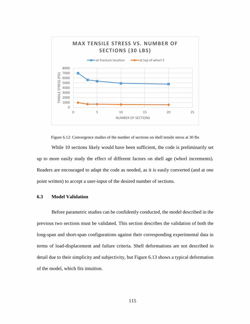
115

Figure 6.12: Convergence studies of the number of sections on shell tensile stress at 30 lbs

While 10 sections likely would have been sufficient, the code is preliminarily set

up to more easily study the effect of different factors on shell age (whorl increments).

Readers are encouraged to adapt the code as needed, as it is easily converted (and at one

point written) to accept a user-input of the desired number of sections.

6.3 Model Validation

Before parametric studies can be confidently conducted, the model described in the

previous two sections must be validated. This section describes the validation of both the

long-span and short-span configurations against their corresponding experimental data in

terms of load-displacement and failure criteria. Shell deformations are not described in

detail due to their simplicity and subjectivity, but Figure 6.13 shows a typical deformation

of the model, which fits intuition.

010002000300040005000600070008000

0 5 10 15 20 25

TEN

SILE

STR

ESS

(PSI

)

NUMBER OF SECTIONS

MAX TENSILE STRESS VS. NUMBER OF SECTIONS (30 LBS)

at fracture location at top of whorl 5

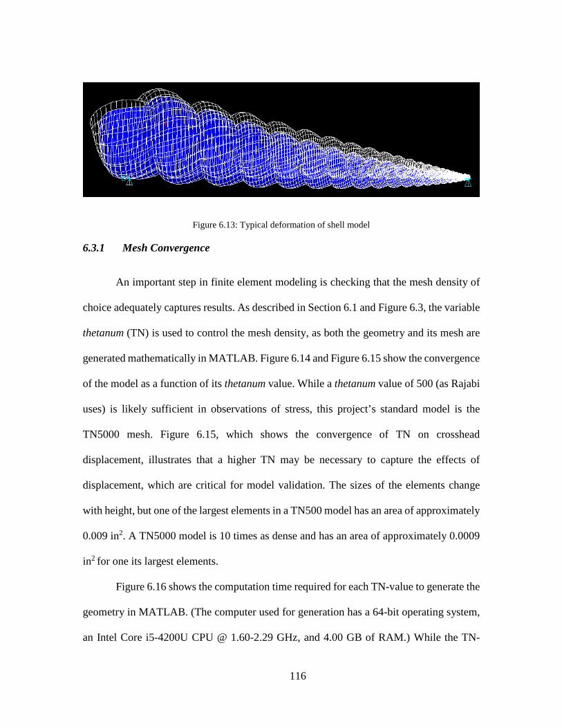
116

Figure 6.13: Typical deformation of shell model

6.3.1 Mesh Convergence

An important step in finite element modeling is checking that the mesh density of

choice adequately captures results. As described in Section 6.1 and Figure 6.3, the variable

thetanum (TN) is used to control the mesh density, as both the geometry and its mesh are

generated mathematically in MATLAB. Figure 6.14 and Figure 6.15 show the convergence

of the model as a function of its thetanum value. While a thetanum value of 500 (as Rajabi

uses) is likely sufficient in observations of stress, this project’s standard model is the

TN5000 mesh. Figure 6.15, which shows the convergence of TN on crosshead

displacement, illustrates that a higher TN may be necessary to capture the effects of

displacement, which are critical for model validation. The sizes of the elements change

with height, but one of the largest elements in a TN500 model has an area of approximately

0.009 in2. A TN5000 model is 10 times as dense and has an area of approximately 0.0009

in2 for one its largest elements.

Figure 6.16 shows the computation time required for each TN-value to generate the

geometry in MATLAB. (The computer used for generation has a 64-bit operating system,

an Intel Core i5-4200U CPU @ 1.60-2.29 GHz, and 4.00 GB of RAM.) While the TN-

117

value used in this project is more exhaustive (and also more computationally costly) than

necessary, the costly MATLAB generation time is a one-time cost, as once the nodes and

elements are generated, the simulation in ANSYS takes only minutes, if not seconds.

Figure 6.14: Convergence studies of mesh density (via thetanum) on shell tensile stress at 30 lbs

Figure 6.15: Convergence study of mesh density (via thetanum) on shell displacement at the loading point

0500

10001500200025003000350040004500

0 1000 2000 3000 4000 5000

TEN

SILE

STR

ESS

(PSI

)

TN#

MAX TENSILE STRESS VS. TN# (30 LBS)

at fracture location at top of whorl 5

-0.003

-0.0025

-0.002

-0.0015

-0.001

-0.0005

00 1000 2000 3000 4000 5000

DISP

LACE

MEN

T (IN

)

TN#

CONVERGENCE OF TN# ON CROSSHEAD DISPLACEMENT

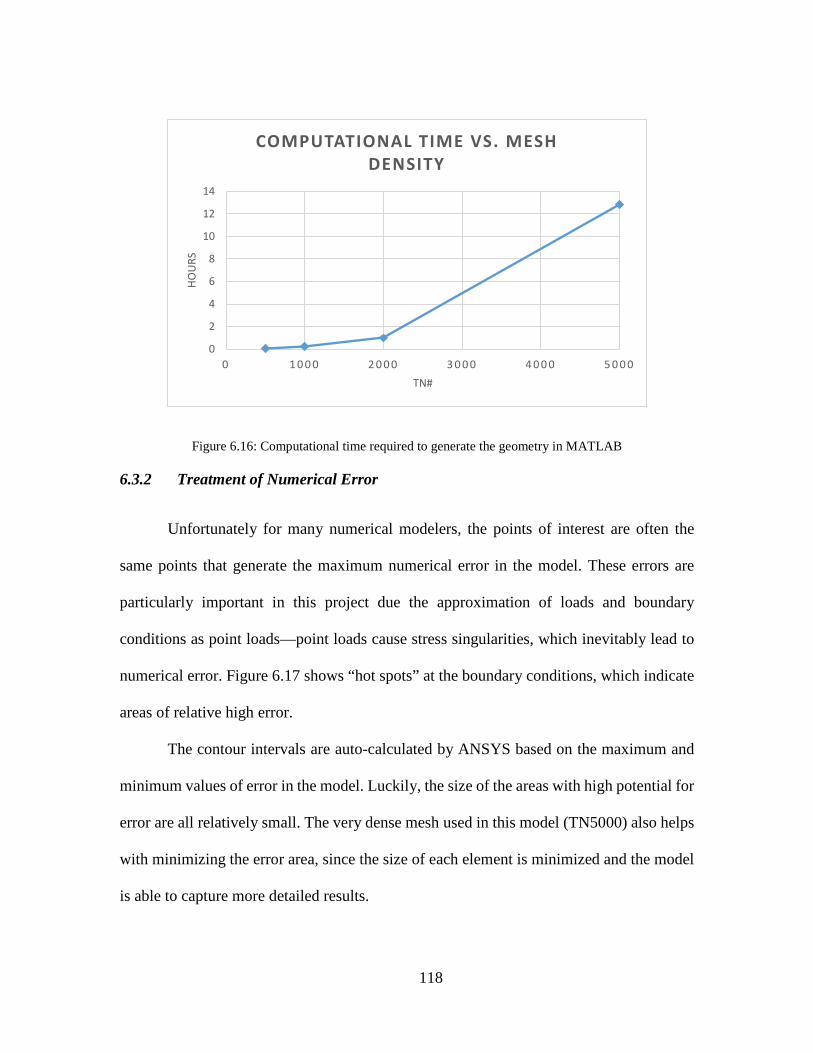
118

Figure 6.16: Computational time required to generate the geometry in MATLAB

6.3.2 Treatment of Numerical Error

Unfortunately for many numerical modelers, the points of interest are often the

same points that generate the maximum numerical error in the model. These errors are

particularly important in this project due the approximation of loads and boundary

conditions as point loads—point loads cause stress singularities, which inevitably lead to

numerical error. Figure 6.17 shows “hot spots” at the boundary conditions, which indicate

areas of relative high error.

The contour intervals are auto-calculated by ANSYS based on the maximum and

minimum values of error in the model. Luckily, the size of the areas with high potential for

error are all relatively small. The very dense mesh used in this model (TN5000) also helps

with minimizing the error area, since the size of each element is minimized and the model

is able to capture more detailed results.

0

2

4

6

8

10

12

14

0 1 0 0 0 2 0 0 0 3 0 0 0 4 0 0 0 5 0 0 0

HOU

RS

TN#

COMPUTATIONAL TIME VS. MESH DENSITY

119

Figure 6.17: Regions of high regions are indicated as “hot spots”, as shown in (a) long-span loading point; (b) long-span base support (no observable error at tip); (c) short-span loading point; (d) short-span supports

However, some numerical error at these point loads is inevitable, and the

unnaturally large “spikes” in simulations need to be responsibly removed. Here, we invoke

Saint-Venant’s Principle and reason that, at a distance far enough away, the manner in

which the load is applied can be neglected; in other words, only in the near vicinity of the

load does the manner of force application have a significant effect on stresses and

displacements. The approach taken here combines the size of the error area (as shown in

Figure 6.17) with the physical, realistic dimensions of the boundary conditions to

determine how large of a radius can be reasonably discounted for reasonable results.

120

Due to the specific way the shell geometry is created in MATLAB, the shape of the

aperture is discretized to form the outer curve of each whorl, and these discretizations can

be seen as the changes in slope along the exterior of the shell. Figure 6.3 in Section 6.1

clearly shows the element edges that rotate with the angle 𝜃𝜃 as the generating curve

revolves around the columella axis. The validated model has 10 of these “ridges” between

the sutures of each whorl. While these edges are not actually raised in the model, they

provide a standard upon which we can gauge area.

The large shells used for validation have about 6-7 ridges per whorl on their exterior

surface, corresponding to approximately 1.5 element edges per physical ridge. As

discussed in Sections 5.2 and 6.2, the shell is reasonably supported by a single ridge at each

boundary condition. Due to the configuration of the short-span setup, we were able to

observe local crushing, to provide physical evidence of the size of the loaded area, without

actually fracturing the shell. Figure 6.18 shows the small area of local failure after only

being loaded up to 35 lbs, indicating that the brunt of the load is distributed over the span

of one ridge. While the long-span shell is allowed to deform in flexure, the short-span shell

does not have the same physical clearance, causing the local crushing of the ridge. (The

crushed area in Figure 6.18 is much smaller than in the similar Figure 5.35 above; while

these are the same shell, this figure shows the damage caused by the boundary constraint

in the linear elastic range while the larger area in Figure 5.35 is after cracking was heard.)

121

Figure 6.18: Local crushing (with no failure) observed in short-span shell after 35 lbs

With this information about ridge-loading, we approximate the disregarded error

area as the span of one physical ridge, or about 1.5 mesh segments. The boundary

conditions in the model are all applied to nodes (which form the corners of elements), so

we take the data within an area created by a half-mesh in all directions to be unreasonable

due to numerical simulation. This “valley to valley” approach is used in approximating

realistic displacements in the model.

The “valley to valley” error subtraction is applied to displacements at all three

boundary conditions, and the adjusted displacements are added to determine the total

simulated displacement, sans numerical errors. Figure 6.19 demonstrates the calculation

for total simulated displacement after some load is applied. The red asterisks represent the

nodes fixed in the y-direction (into and out of the table surface), which are the sources of

numerical error in the supports. These fixed constraints don’t “know” that the rest of the

shell has displaced, causing an unnatural spike in the deformation. The diagram illustrates

122

the short-span shell’s boundary conditions for convenience; the displacements of the long-

span shell are calculated in the same way.

Figure 6.19: Diagram of removal of numerical error in displacements

6.3.3 Long-Span Configuration

This section presents results of the model in comparison to the experimental load-

displacement and failure results described in Section 5.2. A load of 30 lbs is used in the

simulations of displacement, mimicking the 30 lb maximum load applied in the laboratory

experiments. The global stiffness of the shell can then be calculated as the ratio of load (30

lbs) to the y-displacement (in the plane of loading) observed in the shell. The magnitude

of the load at tensile failure is also simulated and compared to failure magnitudes seen in

experiments.

123

6.3.3.1 Load-Displacement Validation

Figure 6.20: Displacement in the direction of loading in the long-span configuration

With a load of 30 lbs, we expect a displacement of 0.003 inches, corresponding to

a stiffness of approximately 10,000 lb/in as found in experimental testing. Figure 6.20

above shows a displacement at the loading point of approximately -0.00269 inches (light

green/yellow contour boundary), after discounting the error caused at this numerically

sensitive area. Similarly, Figure 6.21 below shows displacements at the supports of -

0.691E-3 inches and near-zero at the tip, which is expected due to its distance from the

load. (Furthermore, while the negative displacements here are very small, the pin roller

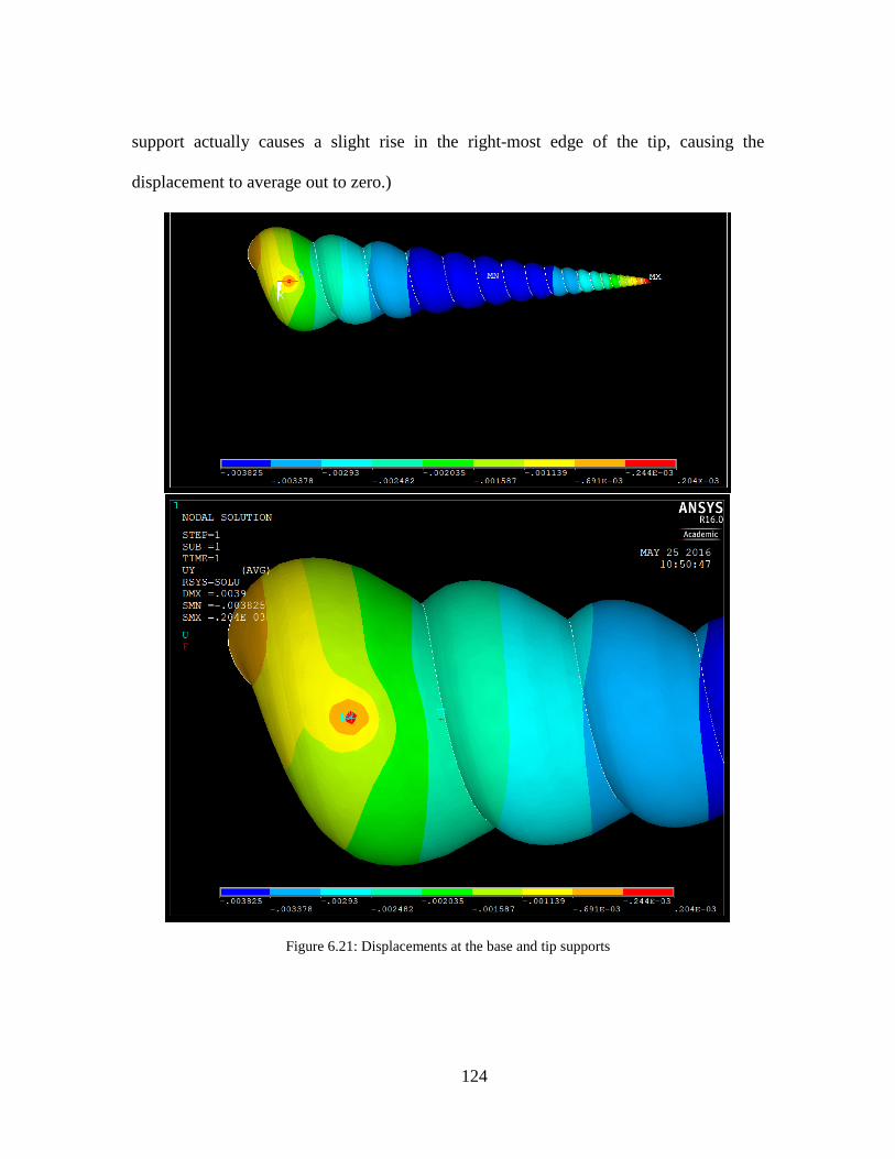
124

support actually causes a slight rise in the right-most edge of the tip, causing the

displacement to average out to zero.)

Figure 6.21: Displacements at the base and tip supports

125

When the displacements of the supports are averaged and summed with the

displacement at the load point (according to Figure 6.19), the total amount of displacement

experienced in the simulated shell is -0.0030355 inches, which leads to a stiffness of 9883

lb/in at a load of 30 lbs. This stiffness value falls well within the range of experimental data

collected for large shells, as shown in Figure 6.22. The blue scatter in Figure 6.22

represents the same data from Figure 5.30, but without differentiating between different

experimental tests.

Figure 6.22: Stiffness value from model (solid black line) falls within range of the load-displacement data collected from experimental testing (blue scatter)

126

6.3.3.2 Failure Criteria Validation

As discussed in Section 5.2.3, the failure loads of the experimental tests ranged

from 39-63 lbs, with an average of 50.6 lbs and a standard deviation of 8.6 lbs. These

failure loads all corresponded to the tip snapping off; this type of failure is consistent with

the location of maximum stresses calculated by the model. Figure 6.23 shows the location

of maximum tensile stress occurring at the suture between whorl 7 and whorl 8, when

counting from the tip. The cut-out view shows a sliver of gray wherein the stress exceeds

the tensile capacity of the shell (5845 psi, as provided by Rajabi’s work), an indication of

tensile failure. We find that maximum stresses near the tip at the "W7t/W8t” interface

exceed the tensile strength of the material at an applied load of 43 lbs.

Figure 6.23: Tensile failure occurs at the bottom surface of shell at 43 lbs at the whorl 7-8 interface when counting from the tip

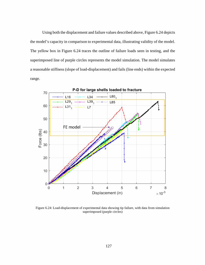
127

Using both the displacement and failure values described above, Figure 6.24 depicts

the model’s capacity in comparison to experimental data, illustrating validity of the model.

The yellow box in Figure 6.24 traces the outline of failure loads seen in testing, and the

superimposed line of purple circles represents the model simulation. The model simulates

a reasonable stiffness (slope of load-displacement) and fails (line ends) within the expected

range.

Figure 6.24: Load-displacement of experimental data showing tip failure, with data from simulation superimposed (purple circles)

128

6.3.4 Short-Span Configuration

While the simulated load in the long-span configuration was limited to 30 lbs, the

experimental tests on the short-span shell demonstrated a linear elastic range up to 170 lbs,

which is used as the simulated load in the discussion below. The adjustment of areas with

high numerical error is repeated with the short-span configuration.

6.3.4.1 Load-Displacement Validation

The displacements found for the short-span configuration are shown in Figure 6.25

and Figure 6.26 below. Note that the gray color in the contour images represent values

outside of the prescribed contour interval. Gray bordered by red represents values higher

than the interval, and gray bordered by blue represents values lower. The interval is

provided at the bottom of each figure. The interval is user-specified in order to provide

more detailed images of local effects at points of interest—the loading point and two

supports.

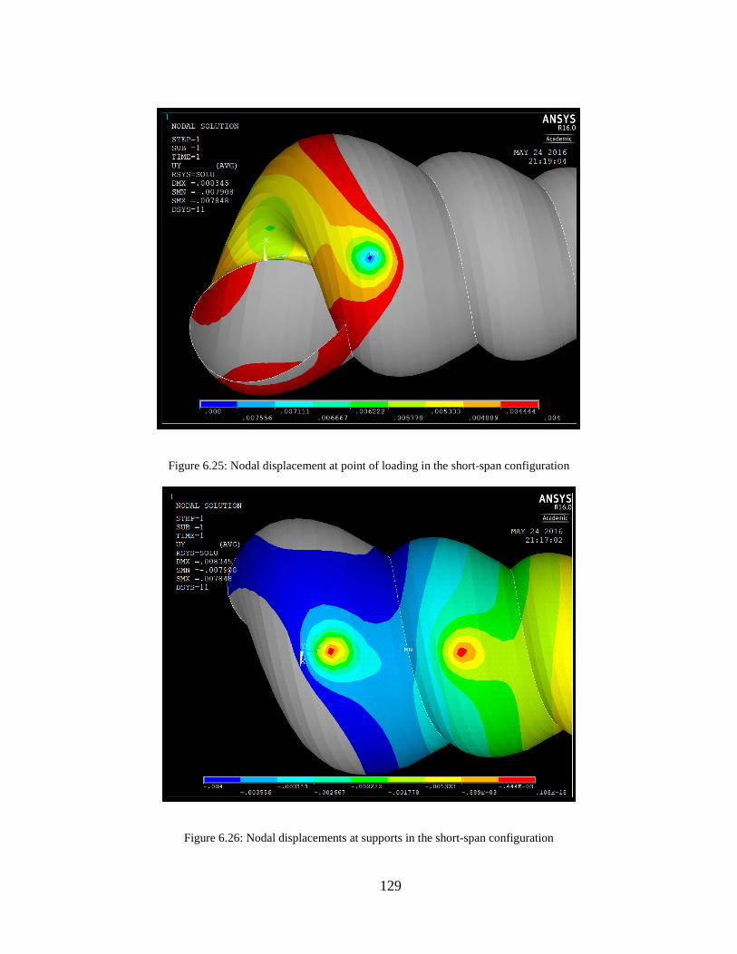
129

Figure 6.25: Nodal displacement at point of loading in the short-span configuration

Figure 6.26: Nodal displacements at supports in the short-span configuration

130

After accounting for numerical error, a displacement of approximately -0.007111

inches (boundary of mid-blue and light blue contours) is simulated at the point of loading.

At the supports, the body whorl has a displacement of approximately -0.001778 inches

(dark green/light green contour boundary) and the adjacent whorl of approximately -

0.001333 inches (light green/yellow contour boundary). The total summed displacement is

then -0.0086665 inches.

This simulated displacement leads to a stiffness value of 19616 lb/in, which is

within 4% of both experimental stiffnesses. Figure 6.27 shows the trendlines of the two

trials, with stiffnesses (slopes) of 18898 lb/in and 18943 lb/in, respectively.

Figure 6.27: Comparison of experimental and simulated load-displacement data in the short-span configuration

Trial 1y = 18898xR² = 0.9962

Trial 2y = 18943xR² = 0.9935

020406080

100120140160180200

0 0.001 0.002 0.003 0.004 0.005 0.006 0.007 0.008 0.009 0.01

LOAD

(LBS

)

DISPLACEMENT (INCHES)

COMPARISON OF P-D EXPERIMENTAL AND SIMULATION DATA

Trial 1 Trial 2 Simulated

Simulatedy = 19616x

131

6.3.4.2 Failure Criteria Validation

As described in Section 5.2.6, the short-span shell experienced some local crushing

at the loading point even though no evidence of failure was captured in the data. Moreover,

the shell was able to withstand a much larger load (~170 lbs) in the short-span configuration

than in the long-span case (~30 lbs). During simulation, the stresses found at the loading

point (7000 psi, conservatively) were larger than the material’s tensile capacity (5845 psi),

even after accounting for numerical errors. Yet, after these curious differences, the crushed

area mimics the damage occurred on the physical shell rather closely. The damage after

maximum load is reproduced in Figure 6.28, along with the tensile stresses predicted by

the model.

Figure 6.28: Large tensile stresses at loading point in short-span shell compared to damage on physical specimen

132

The increased load capacity of the shell in the short-span configuration may be due

to confinement effects caused by the boundary conditions being closer together. In a study

of biaxial stress on concrete samples, Kupfer, Hilsdorf, and Rusch (1969) found that equal

compression in two principal directions can increase the material strength by 80-350%.

Concrete, a brittle material like the shell, is commonly used in engineering applications,

and this phenomena of confinement in brittle materials may elucidate why the stresses

observed in the short-span model are higher than the tensile strength of calcium carbonate.

Also, the similar locations of highest stresses in the model and physical specimen are

promising.

The differences between what was observed during testing and in the model in the

short-span configuration can be summarized as follows:

1. Local crushing of the external ridges was observed during testing but was

not captured in the load data. This may be due to the redundant load paths

in the shell; the shell’s ability to stay intact is not reliant on merely the

ridges. If the test were continued after the sounds of cracking, the failure

likely would have been captured as a small dip in the load data.

2. The short-span model underestimates the enhanced tensile capacity of the

material, since the physical specimen has extra confinement while

confinement is not considered in the model. Taking this into account, the

model and lab failures correlate well.

133

CHAPTER SEVEN

PARAMETRIC STUDIES

The parametric studies that are conducted are designed around the survival goals of

the mollusk. From Section 4.1, we know that the mollusks’ primary predator is the lip-

peeling crab, which has pincers that aim to “peel open” the spiraled shell, and that are also

very effective at crushing the shell to get to the soft-body hiding inside. We also know that

the mollusk lives in sandy mud at the bottom of a body of water, so its streamlined shape

is likely important for limiting drag for mobility.

The mollusk’s presumed survival goal is to not become prey, and it provides

immediate protection for its soft body by preventing fracture at its body whorl. It also aims

to prevent fracture along its spire to ensure its most efficient mobility (drag is optimized

with a non-truncated spire). Thus, the mollusk’s survival can be boiled down to one

characteristic: optimized strength, dependent on location.

One interesting characteristic of the shell is that the immediate threats presented at

the body whorl slowly shift to no longer being life-threatening as the shell grows. In other

words, what used to be a body whorl is gradually left behind as just another point on the

spire as the shell adds more material and internal living capacity over time.

Therefore, three primary variables can be seen as tradeoffs in the generation of the

shell: the total shell mass that the snail has to maneuver, volumetric capacity (living space

for the snail in its body whorl), and minimizing drag. To study their relationships between

each other and to the shell’s load capacity, the shell’s wall thickness is the parameter which

is incrementally changed in the studies below, as it plays a role in two of the three variables.

134

The unfortunate reality for the mollusk is that an increase in load capacity can be achieved

by an increase in thickness, but this also results in a less maneuverable mass. Similarly,

living space can be optimized with thin walls or larger diameters; however, the first leads

to lower load capacity and the second to an increase in mass (--both undesirable). The

geometric variables which determine mass and living space also have tradeoffs with fluid

drag. These relationships are presented with details in the following sections.

7.1 Review of Parametric Variables

Figure 7.1: Review of basic terminology and growth coordinate system

Recall some basic features of the shell (Section 4.1.2): the tip of shell is used as the

origin, and increases in age are represented by increasing distance from the tip (Figure 7.1).

The mass, volumetric capacity, and drag concepts discussed below refer to the broken

length of the spire, the cumulative mass, and the increasing volumetric capacity that change

as the shell grows.

As discussed in Section 5.1.3, the cumulative mass of the shell was determined by

a dividing a collection of different specimen into 1-inch segments. The power laws for each

of the different shell sizes are shown in Figure 5.8, and the equation for large shells is used

in the following parametric studies. These same truncated sections were then used to find

the base diameter at each height as the shell grows. Cross-sectional base diameter as a

135

function of height is given in Figure 7.2. In general, the base diameter increases as the shell

ages (x-axis increases).

Figure 7.2: Base diameter as a function of height

Note that these diameters are measured to the outer surface and only at the sectional

cuts, which were not necessarily at the widest portion of each whorl. The yellow trendline

in Figure 7.2 depicts the total base diameter of shells as a function of their mature size (as

calculated from the total ~200 sample population), which would ideally line up with the

final (mature) data points of each shell size. The inconsistency in the location of the section

cut may account for this slight difference. Note that in both the cumulative mass figure

(Figure 5.8) and the base diameter figure, the trendline of at least the large shells is

Large shells:y = 0.253x + 0.0194

R² = 0.9976

Medium shells:y = 0.222x - 0.0072

R² = 0.996

Small shells:y = 0.21x + 0.029

R² = 0.9959

For mature shells of all sizes:y = 0.1444x1.2999

R² = 0.7102

0

0.2

0.4

0.6

0.8

1

1.2

1.4

1.6

0 1 2 3 4 5 6

BASE

DIA

MET

ER

DISTANCE FROM TIP (INCHES)

BASE DIAMETER ACROSS AGES AS A FUNCTION OF HEIGHT

Large Medium Small Final BD vs. Total Height

136

distinctive from those of the other sizes. This difference between size trendlines further

justifies our claim that shell size and shell age are distinct categorizations (Section 5.1.2).

Base diameter is revisited here because its empirical equations are used in the

calculation of the shell’s volumetric capacity. Internal volumetric capacity (also referred

to as “living space” for the snail) is approximated as a sphere at the body whorl. While the

spiraling growth of the shell causes whorl cross-sections to be slightly offset, this

approximation assumes that the snail gives itself half of the body whorl to live in at any

given time. The base diameter is measured from the exterior, but the radius used for the

sphere of living space discounts the thickness of the wall to give a more appropriate

approximation of inner volumetric capacity (see Figure 7.3).

Figure 7.3: Diagram showing the different measurements used for base diameter and living space

7.2 Effects of Volumetric Capacity-to-Mass Ratio, Shell Age, and Load Capacity

It seems likely that the snail would like to maximize its amount of living space and

reduce the total weight that it needs to manage for optimized “living convenience”; humans

face similar challenges in building and city design. In both of our species, it is desirable to

have maximized function for minimized materials. In the shell, both of these ideals can be

accomplished by having thin walls, but a decrease in wall thickness also makes the shell

137

easier to break (Etter, Denny, and Gaines 2007). The effect of the volumetric capacity-to-

mass ratio on strength is discussed here as a function of shell age, as thickness is

incrementally modified. Thickness is the parametric variable in this effort to capture

relationships between four dimensions.

7.2.1 Incrementing Thickness

Using the thickness relationship from Equation (5) as a baseline, the wall thickness

of a mature large shell was varied as a percent change in thickness throughout the entire

shell length (i.e., a 5% increase in thickness is represented as 1.05*Equation (5). The

change in thickness was repeated for pubescent and young large shells to study the effect

of shell age on strength and living convenience. Logically, an increase in wall thickness at

any point would increase the load the shell is able to withstand before fracture, while

decreasing the available living space and increasing the total shell mass.

The figures below are illustrated as contour plots, where two parameters are

detailed on the x- and y-axes, while a third parameter is shown as a contour plot. In each

case, the data for 0% change in thickness is shown as red stars. Other labels are provided

at the 19.75-whorl marking (representing the validated model): red circles indicate the ±5,

10, 15, and 20% changes in thickness, and the +20% change in thickness is labeled as a red

X to provide the reader with a sense of direction. The “failure load” is the magnitude of the

load that causes maximum principal tensile stress to be equal to the material tensile

strength. While the location of failure is shown to shift between shell ages (discussed below

in Section 7.2.3), it is found to always occur at the bottom plane of the shell (much like a

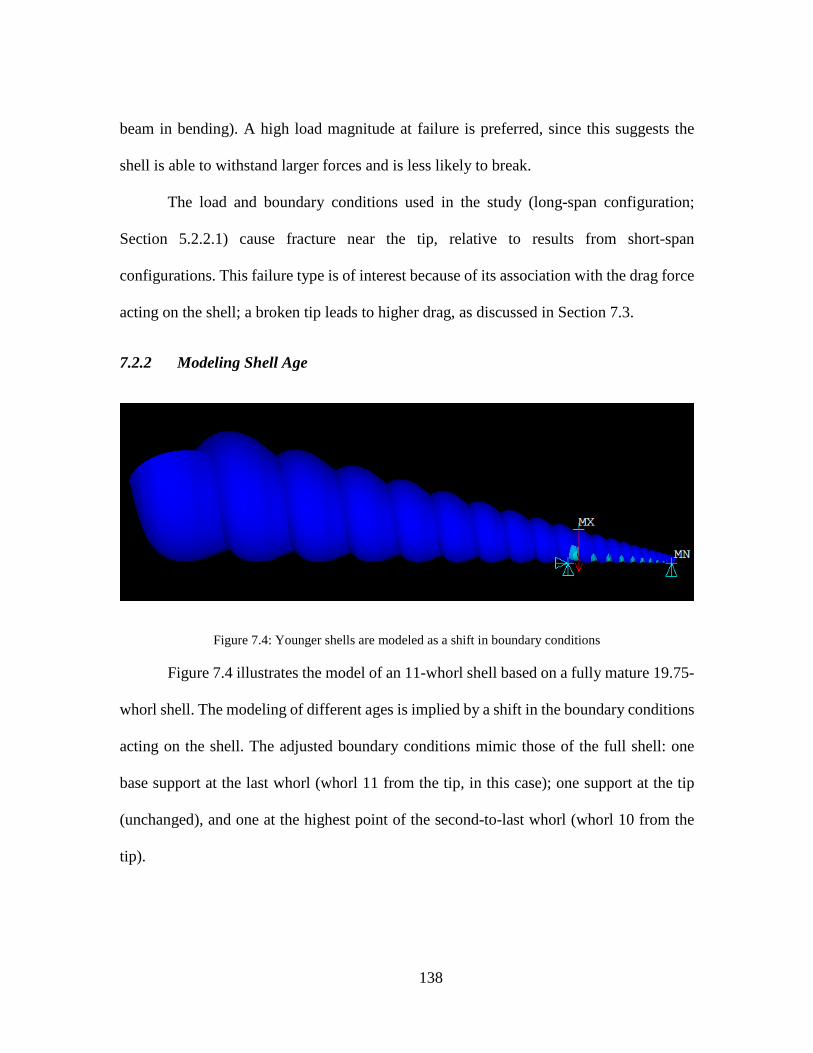
138

beam in bending). A high load magnitude at failure is preferred, since this suggests the

shell is able to withstand larger forces and is less likely to break.

The load and boundary conditions used in the study (long-span configuration;

Section 5.2.2.1) cause fracture near the tip, relative to results from short-span

configurations. This failure type is of interest because of its association with the drag force

acting on the shell; a broken tip leads to higher drag, as discussed in Section 7.3.

7.2.2 Modeling Shell Age

Figure 7.4: Younger shells are modeled as a shift in boundary conditions

Figure 7.4 illustrates the model of an 11-whorl shell based on a fully mature 19.75-

whorl shell. The modeling of different ages is implied by a shift in the boundary conditions

acting on the shell. The adjusted boundary conditions mimic those of the full shell: one

base support at the last whorl (whorl 11 from the tip, in this case); one support at the tip

(unchanged), and one at the highest point of the second-to-last whorl (whorl 10 from the

tip).

139

Figure 7.5: Side view of a 17-whorl shell (top), and a bottom view of an 11-whorl shell (bottom) show that simply shifting boundary conditions is a reasonable method for modeling younger shells

Note that leaving the yet-to-exist length intact does little to affect the younger shell.

Figure 7.5 details the stresses in a younger shell, showing that the length to the left of the

base support is largely inconsequential, even though the cantilever end adds some

unrealistic stiffness to the system. Not only are the stresses low (relative to the failure point)

in the extra length, but we can invoke St. Venant’s principle and claim that the extra stresses

are far enough away from the points of interest to have no effect. One way to confirm the

insignificance of the cantilever is to change the thicknesses of the cantilever sections to be

effectively zero (0.0001 inches), which removes its stiffness and ensures that no forces are

propagated through it. Figure 7.6 shows the stresses produced with the effectively zero

thickness. The stress profiles of leaving the yet-to-exist length intact and “removing” it are

similar, so we have confidence that its effects are negligible in the following studies.

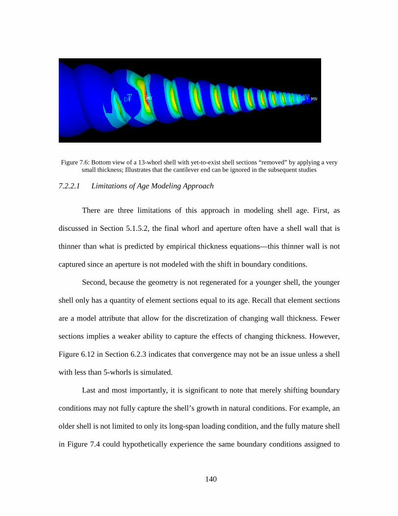
140

Figure 7.6: Bottom view of a 13-whorl shell with yet-to-exist shell sections “removed” by applying a very small thickness; Illustrates that the cantilever end can be ignored in the subsequent studies

7.2.2.1 Limitations of Age Modeling Approach

There are three limitations of this approach in modeling shell age. First, as

discussed in Section 5.1.5.2, the final whorl and aperture often have a shell wall that is

thinner than what is predicted by empirical thickness equations—this thinner wall is not

captured since an aperture is not modeled with the shift in boundary conditions.

Second, because the geometry is not regenerated for a younger shell, the younger

shell only has a quantity of element sections equal to its age. Recall that element sections

are a model attribute that allow for the discretization of changing wall thickness. Fewer

sections implies a weaker ability to capture the effects of changing thickness. However,

Figure 6.12 in Section 6.2.3 indicates that convergence may not be an issue unless a shell

with less than 5-whorls is simulated.

Last and most importantly, it is significant to note that merely shifting boundary

conditions may not fully capture the shell’s growth in natural conditions. For example, an

older shell is not limited to only its long-span loading condition, and the fully mature shell

in Figure 7.4 could hypothetically experience the same boundary conditions assigned to

141

the 11-whorl shell, among infinite combinations of others. However, the opposite is not

true—an 11-whorl shell could not be subjected to the long-span loading of a fully mature

shell (because those whorls do not yet exist). Thus, this age modeling approach only

captures only a subset of growth effects, as shells are necessarily limited to loading effects

on their current size.

As discussed at the beginning of this chapter, the mollusk has two goals: prevent

failure along its spire and at its body whorl. The load capacities in the following study are

only drawn from the long-span configuration, suggesting results about the shell’s spire

failure. Future work will investigate the short-span configuration as well to observe if there

are any differences in parametric effects when the mollusk’s focus shifts to protecting its

body whorl. Therefore, the following studies refer to “age” in a specific context: age is tied

directly to the long-span loading condition which applies boundary conditions at the

extreme ends of the shell.

7.2.3 Shifting Locations of Failure with Age

Figure 7.7: Failure location in a whorl-13 shell shifts to whorl 12-13 interface, whereas older shells have a consistent tip failure at the whorl 7-8 interface

142

An interesting phenomenon observed during simulation is the shift of the failure

location as the shell’s boundary conditions move with age. In simulations of large shells

with 9, 11,13,15,17, and 19.75 whorls, the 15-, 17-, and 19.75-whorl shells all failed in

tension at the whorl 7-8 interface. In shells younger than 15-whorls, the failure location

was at the suture between the base support and the loading point—i.e., the age 9-whorl

shell failed at the whorl 8-9 interface; the age 11-whorl shell failed at the whorl 10-11

interface; and the age 13-whorl shell failed at the whorl 12-13 interface (Figure 7.7).

The shifting failure location in younger shells may be attributed to larger shearing

effects due to the overall shorter length, causing failure between the loading point and base

support. A longer shell has more flexibility and the same load application manifests as

global bending rather than shearing. Further studies could investigate why or how the shell

is able to stabilize the failure location at the whorl 7-8 interface after a certain age/length.

(A theory for the potential of a pre-selected location for failure, when necessary, is

discussed in the section below regarding drag optimization.) The location of failure as a

percent of total length at a given age is shown in Figure 7.8 for the six ages simulated in

this study.

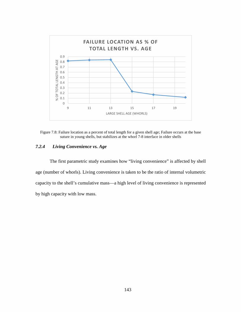
143

Figure 7.8: Failure location as a percent of total length for a given shell age; Failure occurs at the base suture in young shells, but stabilizes at the whorl 7-8 interface in older shells

7.2.4 Living Convenience vs. Age

The first parametric study examines how “living convenience” is affected by shell

age (number of whorls). Living convenience is taken to be the ratio of internal volumetric

capacity to the shell’s cumulative mass—a high level of living convenience is represented

by high capacity with low mass.

00.10.20.30.40.50.60.70.80.9

9 11 13 15 17 19

% O

F TO

TAL L

ENGT

H AT

AGE

LARGE SHELL AGE (WHORLS)

FAILURE LOCATION AS % OF TOTAL LENGTH VS. AGE

144

Figure 7.9: Living convenience increases with age; Contour levels represent the failure load (lbs)

Figure 7.9 shows that a snail’s living convenience increases as it grows—an older

(and perhaps wiser) snail is more efficient at increasing its living space while keeping mass

low. The colored contours in Figure 7.9 illustrate the magnitude of the load that causes

failure. Note that the contour lines follow the load magnitudes, not the percent change in

thickness. The shell is able to withstand larger loads as it gets older, which is simply a

result of static equilibrium assumed in this model. As expected, a shell at any given age

can increase its thickness to decrease its chance for failure, but marginally lose some living

convenience by doing so.

145

The snail may become more efficient at increasing living space while minimizing

mass as it grows, but a simple thought experiment suggests that humans are not as efficient

with our usable space. A common measurement of usable living space in real estate is the

floor area ratio, which measures a building’s total floor area (including stories) as a percent

of its land. Take a skyscraper whose every floor adds area A and mass m – its living space-

to-mass ratio is constant (A/m), unlike the shell. If we consider, instead, volume—in a

direct comparison to the shell—we would find a similar increase of the living space-to-

mass ratio as height (number of floors) increases. However, as much of our vertical space

is unused, this is best characterized as the space that requires heating or cooling. In contrast

to the shell, this is an increasing relationship that we would like to avoid, as it necessitates

an increase in energy costs.

146

7.2.5 Failure Load vs. Age

Figure 7.10: Magnitude of load that causes failure increases with age; Contour levels represent living convenience; Older shells are less likely to break

Figure 7.10 shows that as a shell gets older, the load at which long-span failure

occurs generally increases (regardless of failure location). In other words, older shells are

more resistant to breaking than younger shells are, for the given boundary conditions. In

Figure 7.10, the contours illustrate the effect of a change in thickness on living

convenience; the lighter colors indicate higher living convenience (i.e., high volumetric

capacity to low mass). As expected, a decrease in thickness would both allow for more

147

volumetric capacity and lessen total mass (thus, increased living convenience), but cause

failure to occur more easily (at a smaller load magnitude). Interestingly, the failure load

increases steeply in youth and appears to stabilize after around age 13-15 whorls,

suggesting younger shells are more intent on increasing their load capacity, and that there

may be an upper limit on load capacity.

While older shells are able to resist larger loads than younger shells, this is the

opposite of what we see in human structures. The geometries and structures of shells versus

buildings are obviously very different, but the fact remains that our older structures are

usually in worse condition than newer ones. This is often due to poor upkeep or not meeting

current standards, but structural health does not tend to improve with age. In regards to the

shell’s length as a factor in resisting lateral loads, the simple analogy of building height

can be made. Tall skyscrapers are more vulnerable to lateral loads (like wind) than shorter

structures.

The effect of changing wall thickness also translates well to buildings. Our

engineers could build thinner walls, but likely compromise structural integrity in the

process. Similarly, walls that are overly thick interfere with internal occupant capacity.

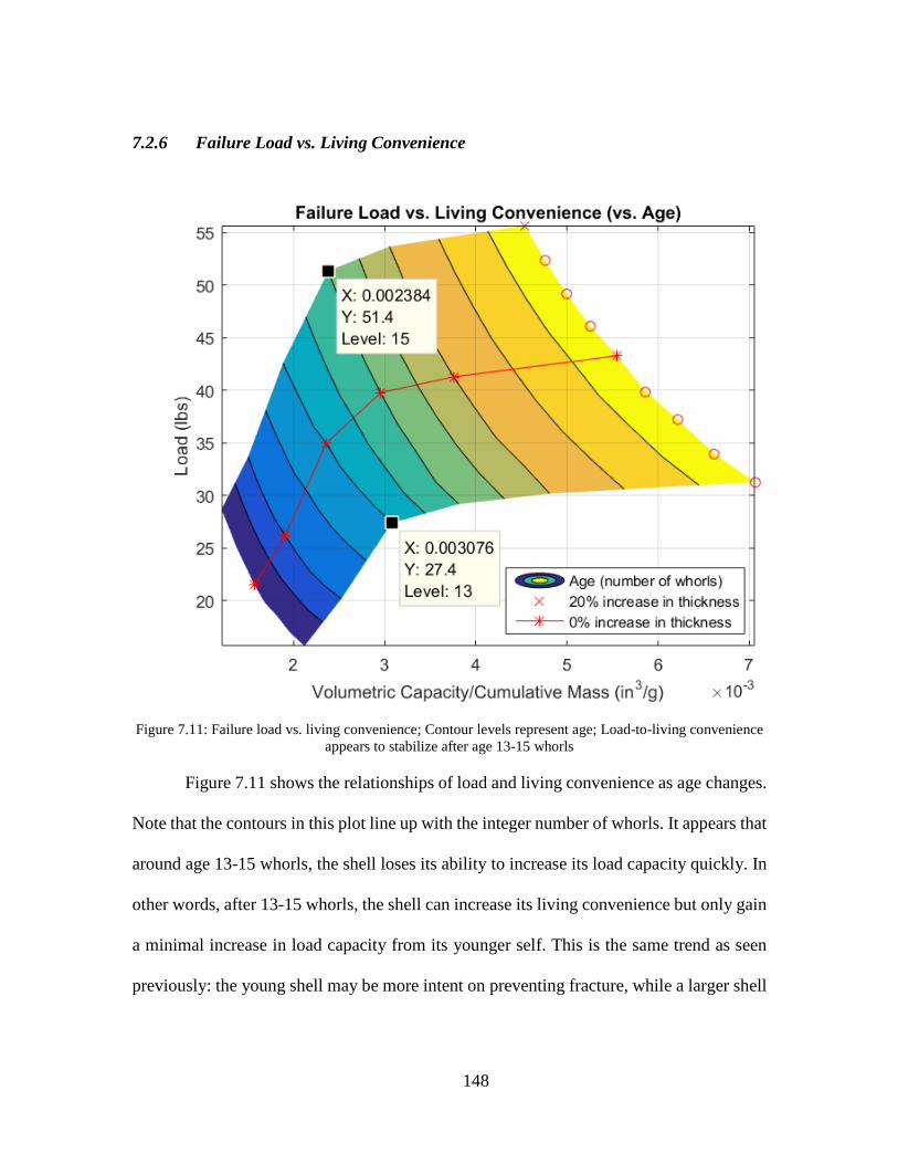
148

7.2.6 Failure Load vs. Living Convenience

Figure 7.11: Failure load vs. living convenience; Contour levels represent age; Load-to-living convenience appears to stabilize after age 13-15 whorls

Figure 7.11 shows the relationships of load and living convenience as age changes.

Note that the contours in this plot line up with the integer number of whorls. It appears that

around age 13-15 whorls, the shell loses its ability to increase its load capacity quickly. In

other words, after 13-15 whorls, the shell can increase its living convenience but only gain

a minimal increase in load capacity from its younger self. This is the same trend as seen

previously: the young shell may be more intent on preventing fracture, while a larger shell

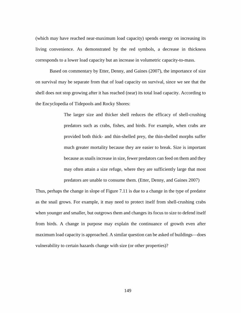
149

(which may have reached near-maximum load capacity) spends energy on increasing its

living convenience. As demonstrated by the red symbols, a decrease in thickness

corresponds to a lower load capacity but an increase in volumetric capacity-to-mass.

Based on commentary by Etter, Denny, and Gaines (2007), the importance of size

on survival may be separate from that of load capacity on survival, since we see that the

shell does not stop growing after it has reached (near) its total load capacity. According to

the Encyclopedia of Tidepools and Rocky Shores:

The larger size and thicker shell reduces the efficacy of shell-crushing

predators such as crabs, fishes, and birds. For example, when crabs are

provided both thick- and thin-shelled prey, the thin-shelled morphs suffer

much greater mortality because they are easier to break. Size is important

because as snails increase in size, fewer predators can feed on them and they

may often attain a size refuge, where they are sufficiently large that most

predators are unable to consume them. (Etter, Denny, and Gaines 2007)

Thus, perhaps the change in slope of Figure 7.11 is due to a change in the type of predator

as the snail grows. For example, it may need to protect itself from shell-crushing crabs

when younger and smaller, but outgrows them and changes its focus to size to defend itself

from birds. A change in purpose may explain the continuance of growth even after

maximum load capacity is approached. A similar question can be asked of buildings—does

vulnerability to certain hazards change with size (or other properties)?

150

7.2.7 Additional Comments on Living Convenience

Two simple relationships are further investigated to corroborate the above theories

of changes in living space. As the shell gets longer, the diameter of the body whorl

increases linearly, which increases the living space available for the snail. Also as the shell

gets longer, the total shell mass the snail carries increases as a power law (Figure 5.8).

Interestingly, when treated as a single variable of living convenience (volumetric capacity

in the body whorl/ total mass), the relationship to growth is linear and positive. Figure 7.12

shows this relationship, indicating that living convenience is constantly increasing and the

snail becomes more energy- and material-efficient with growth.

Figure 7.12: Living convenience increases linearly with age; shell material deposition becomes more efficient with growth

Similarly, we can focus on the optimization of the body whorl instead of taking the

entire shell’s mass into account. Recall that the body whorl is where the snail lives and is

thereby the final whorl at any given age. If we consider the thickness of the body whorl at

y = 0.001x - 0.0001R² = 0.9983

00.0005

0.0010.0015

0.0020.0025

0.0030.0035

0.0040.0045

0.005

0 1 2 3 4 5 6

VOL.

CAP

ACIT

Y/TO

TAL M

ASS

(IN^3

/G)

DISTANCE FROM TIP (IN)

LIVING CONVENIENCE IS IMPROVED WITH AGE

151

a given age, we find that the shell is able to nonlinearly optimize the amount of material it

deposits as it ages (Figure 7.13).

Figure 7.13: Generation of material deposition at body whorl optimizes with age

This increase in deposition efficiency can be thought of as a decrease in the

necessary energy expended by the snail. When the snail is young (short), living space in

the body whorl is sacrificed for more protection (low volumetric capacity-to-thickness

ratio); the young snail expends relatively more energy to deposit thicker walls to protect

itself. As the shell gets older (longer), the volumetric capacity-to-thickness ratio of the

body whorl increases, suggesting that the snail is more energy-efficient as it is able to

increase its living space greatly, relative to the amount of protective material deposited.

These findings may suggest that the snail’s approach is to proactively strengthen

the weaker tip area so that it is less likely to break off later in life. (While quantitative

conclusions were not drawn from the inconsistent measurements, thickness trends in

Section 5.1.5 also indicated a faster rate of thickness generation at younger portions of the

y = 0.001x3 - 0.0005x2 + 7E-05x - 4E-06R² = 1

0

0.02

0.04

0.06

0.08

0.1

0.12

0.14

0.16

0.18

0 1 2 3 4 5 6

VOL.

CAP

ACIT

Y/EN

D TH

ICKN

ESS

DISTANCE FROM TIP (IN)

LIVING SPACE OF BODY WHORL AS SHELL GROWS

152

shell.) The increase in efficiency over time may also point towards a change in the snail’s

survival goals. According to Etter, Denny, and Gaines (2007) above, this trend may suggest

that the snail is in less danger (or exposed to a different danger) as its size increases, and it

changes its deposition habits accordingly.

7.2.8 Summary and Future Directions

The snail’s goals are to maximize its living convenience (i.e., maximize living

space and minimize cumulative mass of shell) and resist breaking forces. The effect of a

percent change in its wall thickness on each of these factors is investigated, and comments

are made as to how these parameters change with shell age. The results of the parametric

studies of volumetric capacity, mass, and failure load are summarized as follows.

• Failure location shifts with age and stabilizes at the whorl 7-8 interface around an

age of 15-whorls. Younger/shorter shells may experience larger shearing action,

while the same force contributes to flexure in longer shells. A study of the sharp

change from shearing to bending (Figure 7.8) is of interest for future studies.

• The snail becomes more efficient at increasing its living space while minimizing

mass as it grows. However, human buildings (e.g., skyscrapers) have no change in

living space-to-mass as more floors are added. When considering volume instead

of floor area ratio (a real estate term), we see a similar increase with growth, but

this is an increase we would like to avoid, as volume is typically only characterized

by energy use (i.e., heating and cooling costs).

153

• While the geometries are different, it is interesting to note that shells are more

capable of resisting lateral loads as they age, while human structures typically

deteriorate with age. The contrast can also be made in units of length—while longer

shells are more capable of resisting lateral loads, our skyscrapers are actually more

vulnerable to lateral loads (e.g., wind) than shorter structures are.

• When the shell reaches 13-15 whorls, the increase in load capacity stabilizes, but

the shell continues optimizing its living convenience. This may suggest an upper

limit on load capacity, and also point to a change in the snail’s intent as it gets older.

A young shell may be more focused on preventing fracture and reaching its load

capacity, while larger shells (which may be approaching the upper limit) instead

spend their energy on increasing living convenience. Or, a young snail may be

vulnerable to different predators than a large snail is. A similar change in purpose

can be considered of buildings—does vulnerability to certain hazards change with

size (or other properties)? If so, is this mid-growth transformation something we

can design for?

• In considering only the body whorl, the snail appears to optimize living space while

decreasing material deposition. This optimization suggests the snail needs or values

protection less when larger, which may be related to a changing purpose as

described previously.

Note that all of the above conclusions are drawn for a large shell, and its failure

loads are found from a long-span simulation which fails due to bending. Further studies on

base crushing are likely to point to interesting results as well, as the base is much more

154

resistant to crushing failure than the tip (e.g., as shown in short-span tests). Future studies

could also use multi-objective optimization to investigate whether the snail weights the

importance of its survival criteria (living space, mass, load capacity), and how these

weights change through growth.

7.3 Effects of Shell Truncation on Drag

It seems likely that drag is an important parameter in determining the optimum

shape of the shell. Whether for mobility or preventing dislodgement, a streamlined shape

helps with reducing the forces of the ocean on the shell and gives the snail more control

over where it would like to locate itself. In reality, the pronounced divots between each

whorl, and the minor ridges along each whorl, likely cause significant turbulence.

However, the overall conical shape is approximated as such in this study to illustrate very

simplified global behavior. (The Turritella is commonly referred to as a “conical shell” as

a reference to the type of gastropod.)

Intuitively, one can imagine that a truncated streamlined shape would have larger

drag than a fully streamlined shape. This section investigates whether the shell has a

predetermined failure location that allows for optimized living conditions after truncation,

if spire failure is inevitable. However, due to the precision needed in fluid drag calculations

(which are typically acquired by empirical studies), the hypothetical case can be

demonstrated by a three concepts.

In approximating the shape of and truncation effects on the shell, the shell form can

be demonstrated as a series of extreme shapes. First, in an actual study of gastropod form,

155

Palmer (1980) approximates the shell as a “sphere of length L”, or an oblong, ellipsoidal

sphere. Palmer’s study is reiterated here for the Turritella terebra, a species not covered

his literature. Second, a first-order approximation is made in Section 7.3.2 to illustrate the

effect of truncation on the drag of a generic streamlined shape, to simulate an increasingly-

broken shell. Finally, the general trends of truncation length on total drag are corroborated

by studies conducted in the automobile industry.

7.3.1 Ellipsoidal Spheres, as Found in Gastropod Literature

While some of Palmer's (1980) approximations and input values seem questionable,

it appears to be the only drag approximation available for gastropod shells. Perhaps a “drag

approximation” is innately futile due to the complexity of fluid flow, but nevertheless, this

section follows Palmer’s drag coefficient calculations. These coefficients are derived from

an empirical relationship between the drag coefficient (Cd) and Reynolds number (Re)

determined by Tietjens (1934), for spheres. The relevant sections of that empirical

relationship are reproduced in Figure 7.14.

156

Figure 7.14: Drag coefficient vs. Reynolds number for spheres (reproduced from Tietjens (1934))

Reynolds number is calculated as

𝑅𝑅𝑚𝑚 =𝑣𝑣𝐿𝐿𝜈𝜈

(6)

where 𝑣𝑣 is the maximum velocity of the object relative to the fluid, 𝐿𝐿 is a

characteristic linear dimension (in this case, the length of the shell), and 𝜈𝜈 is the kinematic

viscosity of the fluid (0.010 cm2/s for seawater). Following Palmer’s footsteps, the

maximum velocity 𝑣𝑣 is taken to be the crawling speed of the mollusk, as identified by

Linsley (1978). While the values in Linsley’s study are suggested to be in units of cm/hr,

his actual units are unclear. Perhaps due to this ambiguity, Palmer assigns units of mm/s to

the same magnitudes of speed, which introduces tremendous error (a scaling factor of 360

between conventions). However, this study adopts Palmer’s mm/s with only this note on

the discrepancy, as we have found no errata produced for either study, and have no

knowledge of whether Palmer and Linsley were in contact.

y = 0.0003x2 - 0.0539x + 3.3984R² = 0.999

00.5

11.5

22.5

33.5

4

0 20 40 60 80 100 120

DRAG

CO

EFFI

CIEN

T

REYNOLDS NUMBER

CD VS. REYNOLDS NUMBER(ADAPTED FROM TIETJENS, 1934)

157

In Linsley’s study of gastropod locomotion rates, he ranks each gastropod species

based on their bilateral symmetry (1 being symmetric, and 3 being asymmetric) and degree

of ornamentation (1 being smooth, and 3 representing nodes or spines). The total “rank” of

each species is calculated by adding the value in the two categories, and he hypothesizes

that Rank 2 shells are the most streamlined while Rank 6 shells offer the most resistance.

Linsley creates an additional Rank 7 category for “shell-draggers”, the slowest snails of

all. According to Signor (1982), the Turritella is a primarily sedentary gastropod, and thus

would likely have been characterized as a shell-dragger by Linsley. Linsley indirectly

confirms this in his 1977 paper by mentioning that Turritellidae are infaunal (live in the

sediment at the bottom of a body of water) high-spired forms, and then mentioning in his

1978 paper that “[a different species] is so high-spired, according to a 'corollary of

Linsley’s Third Law,’ they must have been shell-draggers.” (If T. terebra were not a shell-

dragger, my guess would be that it would fall into Rank 3 of 6, according to Linsley’s

subjective categorization, in comparison to the species he included in his study.)

While Linsley did not measure the speed of the Turritella terebra species, we can

infer that it is very likely a shell-dragger. Thus, the crawling speed of the Turritella is

approximated here as the average of the speeds provided by Linsley for shell-draggers,

0.35 mm/s (Palmer’s units).

Given a maximum shell length of 5.75 inches in the sample population used in this

dissertation, the Reynolds number of T. terebra shells ranges from 0 to 51, according to

Equation (6). Then, using Tietjen’s empirical relationship for the drag coefficient of

spheres (Figure 7.14), this spherical approximation results in drag coefficient values

158

ranging from 2.1 to 1.4, as the length of the ellipsoidal spherical shell increases. Reynolds

number has a linear relationship with shell length (Figure 7.15, top), so we can represent

drag coefficient as a function of shell length (Figure 7.15, bottom).

Figure 7.15: Reynolds number is proportional to shell length (top), so Cd can be represented as a function

of shell length (bottom)

While the purpose of this study was to investigate the effect of shell growth or shell

breakage on drag, it is apparent that this approach does not adequately capture changes in

shell form—the change in length represented above could be used to ambiguously

y = 8.8897x1

R² = 1

0

20

40

60

80

100

120

0 2 4 6 8 10 12

RE

SHELL LENGTH (INCHES)

RE VS. LENGTH

y = 4.2512x-0.609

R² = 0.9976

0

0.5

1

1.5

2

2.5

3

3 3.5 4 4.5 5 5.5 6

CD

LENGTH (IN)

DRAG COEFFICIENT DECREASES AS ELLIPSOIDAL SPHERICAL SHELL GETS LONGER

159

characterize shell size or age just as well as it illustrates truncation. For example, a 50%

truncated shell would have the same drag value as either small or young shells of 50% final

length.

While modeling a turritelliform shell as an oblong sphere is obviously unrealistic,

this approach follows Palmer’s closely. Moreover, Palmer justifies doing so by referencing

a study that compares the Cd/Re value of cephalopod shells to spheres Chamberlain and

Westermann (1976) and suggests that this error is “probably slight.”

7.3.2 First-Order Approximation of Streamlined Shape

A second approach is proposed here that is able to capture the effects of truncation.

By approximating a streamlined form with simple geometry, the streamlined tail can be

truncated at any length, and a first-order approximation can be made of the resulting drag

coefficient. While this approach uses the empirical height, diameter, and angles of the shell

sample population, it is important to note that this approach does not originate from either

gastropod or drag experts.

The common streamlined shape is well-described in literature for objects with a

Reynolds number of approximately 104. (Recall from Section 7.3.1 that T. terebra shells

are approximated to have a Reynolds number range of only 0-51, and note, again, that this

approximation is a vast generalization to show only the trends of truncation.) While the

degree of being streamlined is characterized purely by fluid flow, streamlined forms in

general (also known as the “teardrop” shape) can be reasonably approximated as a

hemisphere attached to the base of cone, where the tip of the cone is at the tail end of fluid

160

flow (see Figure 7.16). We are given in literature (for Re ≈ 104) that the drag coefficient

for a hemisphere is 0.42, and that of a teardrop is 0.04. In a first-order approximation, the

allowable range of drag coefficients, as a function of truncated length, is limited to these

extremes: a fully streamlined shape (0.04) and a completely truncated spire, leaving just a

hemisphere (0.42).

Figure 7.16: 2D projection of hemisphere plus cone approximation of streamlined shape

Figure 7.16 shows the different dimensions of the approximated geometry. The full

length L, base radius (and hemisphere radius) r, and angle 𝜃𝜃 are from the average

measurements of the sample population. Because 𝜃𝜃 stays constant for a given shell even

after breaking, this angle is crucial in determining the radius at the broken edge. The drag

coefficient can be found by interpolation between the two extremes,

𝐿𝐿𝑑𝑑 = 0.04 + 0.38 ∗ �𝐴𝐴𝑡𝑡𝑟𝑟𝑡𝑡𝑡𝑡𝑡𝑡𝐴𝐴𝑏𝑏𝑏𝑏𝑠𝑠𝑏𝑏

� (7)

where Atrunc is the circular area at the truncated end, and Abase is the circular area of

the hemisphere. By simple substitution,

161

𝐴𝐴𝑡𝑡𝑟𝑟𝑡𝑡𝑡𝑡𝑡𝑡 = 𝜋𝜋𝑚𝑚22 = 𝜋𝜋(𝑚𝑚 − 𝑚𝑚1)2 = 𝜋𝜋(𝑚𝑚 − 𝐿𝐿𝑡𝑡𝑟𝑟𝑡𝑡𝑡𝑡𝑡𝑡 tan(𝜃𝜃))2. (8)

Knowing the area of the hemisphere face and substituting Equation (2) into

Equation (7), the first-order drag approximation is

𝐿𝐿𝑑𝑑 = 0.04 + 0.38 �1 − 𝐿𝐿𝑡𝑡𝑡𝑡𝑡𝑡𝑡𝑡𝑡𝑡𝑟𝑟

tan(𝜃𝜃)�. (9)

The following graphs and discussion points investigate the effects of truncation

location on drag and mass, and these are demonstrated across ages (as a single shell adds

more whorls over time). The first point of interest is how the drag coefficient changes as a

function of truncation location. In Figure 7.17, the x-axis indicates the distance from the

tip at truncation, so a larger x-value indicates that a larger portion of the spire has broken

off.

Figure 7.17: Drag coefficient as a function of truncation length from tip

Figure 7.17 shows that older shells, which are longer, have less overall drag than

younger versions of themselves. For example, if 2 inches of spire are broken off a 3.5-inch

00.05

0.10.15

0.20.25

0.30.35

0.40.45

0 1 2 3 4 5

DRAG

CO

EFFI

CIEN

T

DISTANCE FROM TIP AT WHICH FAILURE OCCURS (IN)

OLDER (LONGER) SHELLS HAVE LESS DRAG

Adult large Pubescent large Young large

162

shell, the remaining stub induces much more drag than if 2 inches of spire are broken off a

5.5-inch shell, since the longer shell has more remaining length. Another way to visualize

this is to plot drag coefficient against the percent of length lost, a percent which increases

as more of the spire is truncated (Figure 7.18).

Figure 7.18: Drag coefficient as a function of % length of spire lost

When viewed as a percent of length, we see that the age of the shell no longer

matters, and that ultimately no breakage is ideal (minimum drag). There also is no obvious

optimum in this representation as the “best” location to break, if inevitable.

Finally, the remaining mass versus drag coefficient presents an interesting scenario.

While the snail likely prefers less drag, the desired mass is ambiguous; in the previous

study of volumetric capacity and strength (Section 7.2), mass was assumed to be optimized

when the snail had less to carry around. However, in the context of drag, especially after

the findings from literature (Section 7.3.1) where the Turritella is suggested to be a shell-

dragger, it may be possible that a larger mass helps to prevent the snail from being washed

y = 1E-13x3 + 0.3798x2 + 0.09x + 0.0453R² = 1

00.05

0.10.15

0.20.25

0.30.35

0.40.45

0 0.2 0.4 0.6 0.8 1

DRAG

CO

EFFI

CIEN

T

% OF LENGTH LOST OF SPIRE

DRAG VS. % LENGTH LOSTAdult large Pubescent large Young large

163

away by turbulent waves. Even though a shell-dragger moves minimally, a streamlined

shape could also be a factor in avoiding turbulence. Figure 7.19 illustrates the relationship

of remaining mass and drag coefficient.

Figure 7.19: Remaining shell mass after truncation vs. corresponding drag coefficient at truncation

Figure 7.20: Mass-to-drag ratio vs. percent length lost of total shell length

0

5

10

15

20

25

30

0 0.05 0.1 0.15 0.2 0.25 0.3 0.35 0.4 0.45

MAS

S (G

)

DRAG COEFFICIENT

MASS VS. DRAG COEFFICIENTAdult large Pubescent large Young large

0

100

200

300

400

500

600

700

0 0 . 1 0 . 2 0 . 3 0 . 4 0 . 5 0 . 6 0 . 7 0 . 8 0 . 9 1

MAS

S/CD

(G)

% LENGTH LOST

MASS/CD VS. %LENGTH LOSTAdult Pubescent Young

164

Assuming the theory of maximum mass preferred, a shell would be optimized with

large mass and low drag—which can be characterized as a new ratio variable. Figure 7.20

demonstrates the effect of the percent lost of total shell length on the remaining mass-to-

Cd ratio. While a larger value of mass-to-drag is preferable, a shift to a nonlinear decrease

is seen around 25% of total length lost. However, note that a significant limitation of this

approach is the assumption that shells of all ages can be approximated with the same drag

coefficients at geometric extremes. This is not the case in the physical world, as total length

plays a role in the drag coefficient of the shell (i.e., intact adult/longer shells should have

less overall drag than intact younger/shorter shells).

7.3.3 Kammback Truncation

The automobile industry has historically been a forerunner in the study of

streamlining bodies. While an automobile may have little to do with a seashell, the

literature from this discipline provides examples of the effect of truncation of streamlined

shapes. The Kammback is a car body type designed based on the research of

aerodynamicist Wunibald Kamm, who studied whether the suggestion of a streamlined

shape caused laminar airflow even if the end of the tail was missing (Magazines 1981).

Figure 7.21 (adapted from Hoerner (1951)) provides the drag coefficient for a Kammback

fuselage body as the tail is truncated. The context of the coefficients (e.g., Reynolds

number, fluid flow) are not provided here; however, the increasing effect of drag due to

increased truncation is clear.

165

Figure 7.21: Drag coefficients for a Kammback fuselage body as tail is truncated in 10% increments

The graphical representation of the truncation effect is shown in Figure 7.22. Even

though externalities are bound to be drastically different, the general shape of the curve is

comparable to that found by first-order approximation and shown in Figure 7.18.

Figure 7.22: Graphical representation of Kammback drag coefficients with truncation

y = 4E-07x3 - 7E-06x2 + 0.0002x + 0.0647R² = 0.9995

0

0.05

0.1

0.15

0.2

0.25

0.3

0.35

0.4

0 20 40 60 80 100 120

CD

% LENGTH LOST OF SPIRE

EFFECT OF TRUNCATION ON KAMMBACK DRAG COEFFICIENT

166

7.3.4 Summary and Limitations of Drag Approximations

While all three approaches presented above have considerable flaws and

limitations, the trends of these relationships tell a similar story: the turritelliform shell

functions best when it is mature and intact. It is worth reiterating that while the profile of

the Turritella is approximated as smooth and/or streamlined in all three approaches to

calculating drag, the realistic shell has pronounced divots at whorl sutures, as well as small

ridges along the exterior that follow the path of each generating curve. These accents are

likely to cause significant turbulence not captured in the approximations made above. The

three approaches are summarized as follows:

• The first approach follows Palmer’s (1980) approximation for calculating

the drag of gastropod shells modeled as ellipsoidal spheres. As expected,

we conclude that increasing length corresponds to less drag. Unfortunately,

the approximations made in this approach are inadequate for capturing the

effects of truncation.

• The second approach uses realistic shell dimensions, but unrealistic

Reynolds numbers. A first-order approximation of shows that the drag

coefficient increases as the percent of spire length lost increases. A “critical

point” is found around 25% of total length lost for all shell ages, marking

the transition from linear to nonlinear decrease of mass-to-drag ratio. This

approach is limited by the unrealistic assumption that small and large

streamlined shapes have the same drag coefficients at extremes, such that

drag is only characterized by the shape profile.

167

• The third approach presents findings from the automobile industry to show

empirical values of drag coefficients as a result of truncation of streamlined

shapes. While the contexts are drastically different, the Cd profiles are

similar to those found in the previous approximations of shells.

168

CHAPTER EIGHT

IMPLICATIONS

While the primary goal of this project is application of adaptability lessons from

Nature to the built environment, there are significant secondary implications of this work

in other disciplines as well. The short descriptions below are meant to be thought-

provoking for readers to consider the broad impacts biomimicry and/or adaptability can

have in different contexts. The connections between this research and its potential

applications are presented here.

8.1 Adaptability in Structural Design

There are three approaches in which this research can be applied to structural

design. First, there are on-going studies of adaptable design in human structures, though

practical implementation is currently rare. This may be due to the academic youth of this

body of literature, or that practitioners who do implement adaptability are unfamiliar with

considering their work within a theoretical framework. For example, designing for

adaptability and deconstruction (DfAD or DfD) is a construction approach that emphasizes

the importance of the design stage in considering the life cycle (rather than just the

usefulness) of structural components (e.g., Webster (2007)). While some practicing

engineers may naturally consider the after-life implications of their designs, they may not

know that there is a term for their type of designs (Ross et al. 2016). As the theoretical

classifications of enablers of adaptability (or adaptability parameters) continue to be

outlined, identified, and described, the potential for this research increases. Connections

169

can be drawn between the adaptability lessons drawn from Nature and those that enable

adaptable structures. As translations between Nature and the built environment are

clarified, there is an opportunity to turn to practicing designers and point out specific

characteristics that they can focus on to enable adaptability. This work provides scientific

backing for an enhanced design process through the mathematical characterization of

natural systems, for translation and impact on other types of systems.

Second, the process of characterizing systems with a bottom-up approach—

studying the functions that lead to form—can be repurposed in the built environment for a

rigorous study of the behavior of structures through different lenses. For example, factors

that influence occupant comfort can be considered the simple elements or building blocks

of a successful system. For instance, what is the best layout for a structure that ensures all

inhabitants still have access to natural light, even as its occupant capacity is increased by

the addition of rooms? Or, if we run out of living space and need to build vertically, how

can we redesign structural components so that they can be easily modified when an

unknown number of floors will be added?

Similarly, stakeholders who influence the sequence and choices made for structural

design can be considered individual agents within a complex network leading to the

construction of buildings. Investigating the motivations and actions of these agents, such

as in social or information networks, can lead to a more complete understanding of all the

factors that influence the form of a structure (Klotz, in progress). And, like discussed in

Section 2.3, by distilling the important pieces of a system into simple(r) elements, we gain

170

a fundamental understanding of each agent and can piece them together in different

configurations for different outcomes.

Third, lessons can be learned from the geometric and parametric studies on the T.

terebra for direct application to human structures. For example, while it seems implausible

that buildings will be designed to grow as spiraled towers (for one, they would need to be

upside-down), there are some building features, such as church steeples or mosque

minarets, that have similar forms (Sorguç and Selçuk 2013, e.g., Børsen Copenhagen Stock

Exchange). Depending on the desired functional requirements, structural features can be

informed by natural geometric relationships, or by the parametric growth studies (Chapter

7) for a starting point of functional tradeoffs. For instance, a minaret could use the thickness

equations in Section 5.1.5 to advise schematic designs.

8.2 Informing Urban Planning

As mentioned briefly in Section 2.1.3, there is potential for adaptability at scales

even larger than a structure. City and regional planners are responsible for the layout of our

communities, and the success of a city is heavily dependent on their foresight.

Comprehensive plans (an official document detailing the growth vision of a city) do often

take stakeholders opinions into account, but many of our urban centers are developing wide

expanses of sprawl, which is both a form and cause of unsustainable city growth (e.g., Hall

and Porterfield (2001, Ch. 4)). While city and regional planning may seem far removed

from day-to-day civil engineering, these disciplines ultimately function within the same

body albeit on different hierarchical scales (e.g., Chapter 3), and the designs of each are

171

bound to affect the other. In fact, cities may even be a better analogy for the spiraled

gastropod shell than buildings. Cities, more so than buildings, expand as more space is

needed due to an increase in occupancy, whereas new buildings are typically constructed

when more space is needed, rather than retrofitting an existing one.

While buildings don’t usually increase their efficiency with scale, cities do. For

example, New York is the largest and, yet, most sustainable city in the United States

(Cohen and Richard 2006). We actually see that an increase in population density increases

infrastructural efficiency, since the physical components of infrastructure (e.g., cables,

pipes) have less absolute area to span. On the other hand, Los Angeles is another urban

center but is extremely unsustainable due to its expanses of sprawl. Urban sprawl

stimulates wealth inequality between the urban center and suburbia at the fringe, which in

turn encourages the ownership of private vehicles for traveling long distances. Say, for

instance, municipal funds are distributed to the wealthier urban fridge at the cost of public

transit at the urban center, causing lower income persons to be disadvantaged and have

limited choices in housing and employment due to the layout of their city. City layouts

shape quality of life, and perhaps we can learn from the shell how to grow in a more

equitable way that prevents marginalizing sections of a system for the benefit of others.

There is a long history, from Mumford (1961) to Batty (2013) of studying the form

of human settlements. Recent work (e.g., Bettencourt et al. (2007)) shows that some

fundamental equations can be used to describe human behavior and efficiencies in these

cities. For example, as cities grow, they require fewer resources per capita and produce

more innovations per capita. While such research derives equations from the behavior of

172

cities, this research hints at the potential to use equations to inform the design of cities. As

seen in Chapter 7, the seashell grows in a way that is efficient for its occupant and also

becomes more efficient as it grows. Urban cities grow in an analogous manner—as a city’s

population grows, higher density commercial and residential structures tend to be

constructed, leading to more living space for less material, like the shell achieves. Are there

other lessons we can draw from Nature to apply to the design of growing cities?

8.3 Educating Civil Engineers

While this project may seem far-fetched to some civil engineers, one objective of

this research is to stimulate interest in a new technique within a traditionally conservative

discipline (and for good reason—civil engineers are responsible for protecting lives). Both

the paper on the lessons from coral reef (Chapter 3) and the technical work conducted for

this dissertation on shells are meant to serve as examples of how biomimicry can be more

than conceptual inspiration, and how solutions found in Nature can be structurally

comparable to those developed by humans.

In a more practical sense, biomimicry can also be easily included in introductory

engineering courses, either as its own topic or as a supplement to a design project. In fact,

the author has given single-period lectures on biomimicry to middle and high school

students, as well as at the college and graduate levels. In a design engineering context, the

idea of breaking down an organism into its various biological functions fits in well with

the reverse engineering of designs for the understanding of functions, objectives, and

constraints (Dym and Little 2008, see Figure 8.1).

173

Figure 8.1: Illustration of inserting biomimicry into systems engineering

Biomimicry resources and databases like AskNature.org and TRIZ (see Section 2.2) are

already organized by biological functions, which can substituted into a project’s original

designs rather straightforwardly. A simple requirement to explore parallel functions in

Nature can stimulate students to think more about sustainability and the impact of their

work (e.g., (Kennedy, Buikema, and Nagel 2015)).

8.4 Time-Lapse 3D Printing

The current way 3D printing works is by processing an engineering blueprint for a

product, and dividing it into horizontal cross-sections. These cross-sections are printed by

the deposition of material, layer by layer, building the final creation through a linear

process in one physical dimension. Studies of the growth process of biological materials

may have an impact on the current method for 3D printing, which is considered by many

to be the origin of a technological revolution. However, neither the shell nor human

structures grow in this linear point-by-point fashion. If we can pinpoint how and where an

organism decides to deposit material through time, in such a way that reinforces its

structure, can we strengthen 3D printed materials to mimic this process through a time-

174

lapse blueprint, rather than just the final form? (Could this lead to a type of 4D printing?)

Moreover, the study of growth through time can also be applied to construction methods

to determine the optimized sequence to build a structure. The Robotic Building group at

TU Delft is currently pursuing a similar idea through the investigation of 3D printing

materials that capture microstructure characteristics through form finding and model

optimization (Bier 2014).

8.5 Contributions to Complexity Science

Further investigation in the science of complexity (Section 2.4) may lead to new

discoveries and understanding of sustainability for the built environment. Different types

of theories that contribute to complexity science include scaling and criticality, which

would be a fitting area for the growth of biological systems; adaptation and game theory,

which explores evolution through cooperation and behavioral sciences; and information

theory, which is considered a tool to analyze and understand complex systems (Newman

2011). Many of the concepts explored in this dissertation are based in one of the theories

of complexity, and many others are tools that may be used to continue in this realm of

work. The science of complexity may be an overarching theme in which the concepts in

this research are better connected. The paper by Csete and Doyle (2002) is just one example

of how biological complexity, design engineering, adaptation, and systems thinking can be

combined.

175

APPENDICES

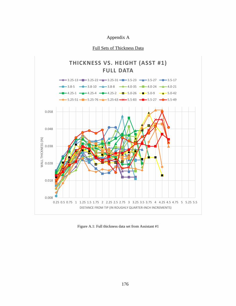
176

Appendix A

Full Sets of Thickness Data

Figure A.1: Full thickness data set from Assistant #1

0.008

0.018

0.028

0.038

0.048

0.058

0.25 0.5 0.75 1 1.25 1.5 1.75 2 2.25 2.5 2.75 3 3.25 3.5 3.75 4 4.25 4.5 4.75 5 5.25 5.5

WAL

L TH

ICKN

ESS

(IN)

DISTANCE FROM TIP (IN ROUGHLY QUARTER-INCH INCREMENTS)

THICKNESS VS. HEIGHT (ASST #1)FULL DATA

3.25-13 3.25-22 3.25-31 3.5-23 3.5-27 3.5-17

3.8-5 3.8-10 3.8-8 4.0-35 4.0-24 4.0-21

4.25-1 4.25-4 4.25-2 5.0-26 5.0-9 5.0-42

5.25-51 5.25-76 5.25-63 5.5-83 5.5-27 5.5-49

177

Figure A.2: Thickness data set from Assistant #1 with sizes grouped

Figure A.3: Full thickness data from Assistant #2

0.0100.0150.0200.0250.0300.0350.0400.0450.0500.055

0 0 . 5 1 1 . 5 2 2 . 5 3 3 . 5 4 4 . 5 5

WAL

L TH

ICKN

ESS

(IN)

DISTANCE FROM TIP (IN ROUGHLY QUARTER-INCH INCREMENTS)

THICKNESS VS. HEIGHT (ASST #1)3.25-avg (n=3) 3.5-avg (n=3) 3.8-avg (n=3) 4.0-avg (n=3)

4.25-avg (n=3) 5.0-avg (n=3) 5.25-avg (n=3) 5.5-avg (n=3)

0.000

0.010

0.020

0.030

0.040

0.050

0.060

0 0 . 5 1 1 . 5 2 2 . 5 3 3 . 5 4 4 . 5 5

WAL

L TH

ICKN

ESS

(IN)

DISTANCE FROM TIP (IN ROUGHLY QUARTER-INCH INCREMENTS)

THICKNESS VS. HEIGHT (ASST #2)FULL DATA

3.25-13 3.25-22 3.25-31 3.5-23 3.5-27

3.5-17 4.25-1 4.25-4 5.5-27 5.5-49

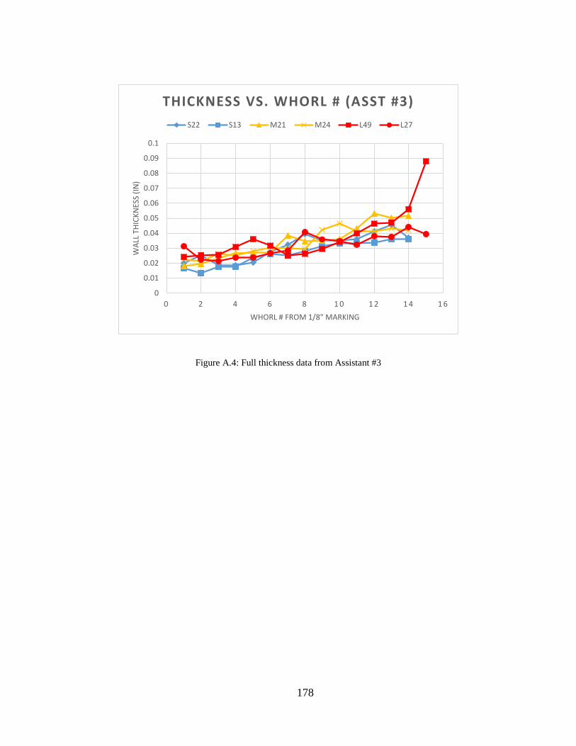
178

Figure A.4: Full thickness data from Assistant #3

0

0.01

0.02

0.03

0.04

0.05

0.06

0.07

0.08

0.09

0.1

0 2 4 6 8 1 0 1 2 1 4 1 6

WAL

L TH

ICKN

ESS

(IN)

WHORL # FROM 1/8" MARKING

THICKNESS VS. WHORL # (ASST #3)S22 S13 M21 M24 L49 L27

179

Appendix B

Cross-Sectional Scans of Shells Used for Thickness Measurements

In the figures below, the borders represent a standard 8.5”x11” piece of paper,

which may act as a scale for researchers interested in using these scans. Shell halves were

placed in an office scanner, and the resulting images were color-inverted to produce the

following images, which are easier to interpret with dark walls and a light background.

While the shells are not sorted in any particular order, the small strips of paper

indicate the shell label and general size category (approximate total length) of each shell

as measured prior to any alteration (discussed in Section 5.1.1). The contents of each figure

are included at the bottom of each page.

180

Shells L27, L49, L63, L76

181

Shells S5, S10, M8, L26, L51

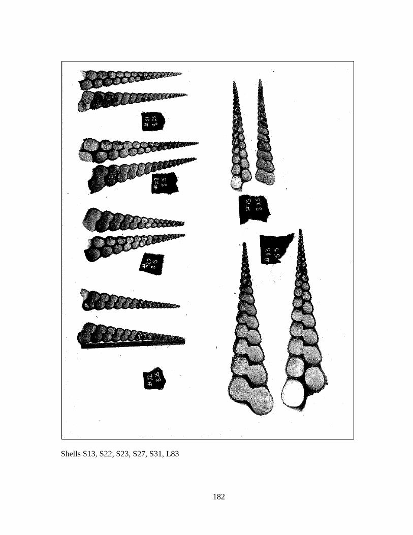
182

Shells S13, S22, S23, S27, S31, L83

183

Shells M1, M2, M4, M21, M24, M35

184

Shells L9, L42

185

Appendix C

DAQ data processing protocol

1. A sampling frequency of 100 Hz is used for both data collection systems.

2. Force data is multiplied by 1.0247, as per the calibration constant we found in

calibrating the UTM load cell to the donut load cell which is connected through the

DAQ.

3. DAQ data (particularly noticeable in strain) is stepwise in increments of 803 data

points per plateau. DAQ data is decimated by 400 to ensure that each plateau is

captured at least once (depending on how long the first plateau is).

4. The decimated data is zeroed and a rudimentary moving average function is

implemented to automatically identify where the test begins. The data is cut at the

first index where the mean of a small window of data is greater than 0.05 lbs.

5. The DAQ data is then low-passed filtered with a 9th order Butterworth FIR and a

cut-off frequency of 1 Hz.

6. The UTM is zeroed before every test. Additionally, each test’s start and end is

controlled (manually) by the force value recorded by the UTM. The DAQ, on the

other hand, is allowed a few seconds at the beginning and end of each test, prior to

and after the stop of UTM driver movement, to “settle down”. These “data tails”

are needed in order to identify where the test begins and ends. These tails are

removed from the data and the data is zeroed based on the initial offset.

186

function [daqnew] = processData(UTMdata, DAQdata) % Use this script to process DAQdata (cut, filter) into data that is % usable for P-D or P-Eps plots % Input: % - Raw UTMdata % - Raw DAQdata DAQdata(:,2) = DAQdata(:,2)*1.0247; DAQdata(:,3) = DAQdata(:,3)*10^6; % Output: new daq vector %% Read data UTMtime = UTMdata(:,1); UTMforce = -UTMdata(:,3); UTMforce = UTMforce - UTMforce(1); DAQtime = DAQdata(:,1); DAQforce = DAQdata(:,2)-mean(DAQdata(1:100,2)); % roughly zero just to see on plot DAQstrain = DAQdata(:,3)-mean(DAQdata(1:100,3)); % roughly zero just to see on plot OrigDAQtime = DAQtime; % these use the roughly zeroed data OrigDAQforce = DAQforce; OrigDAQstrain = DAQstrain; newDAQtime = DAQtime; newDAQforce = DAQforce; newDAQstrain = DAQstrain; % Decimate and filter to find index at which to cut original data % Decimate decimateBy = 400; % Each plateau is 803 pts long DAQforce = decimate(DAQforce,decimateBy); DAQtime = decimate(DAQtime,decimateBy); DAQstrain = decimate(DAQstrain,decimateBy); DAQstrain = DAQstrain - DAQstrain(1); DAQforce = DAQforce - mean(DAQforce(1:5)); % Filter % Apply 9th order butterworth low-pass filter cutoff = 1; % assign this; low pass cutoff value (Hz) order = 9; % assign this

187

fs = 100; % sampling freq (Hz) Wn = cutoff/(fs/2); [b,a]=butter(order,Wn,'low'); DAQstrain = filtfilt(b,a,DAQstrain); DAQstrain = DAQstrain - DAQstrain(1); % Find the first index in DAQforce that is non-zero nonZeroFlag = 1; while nonZeroFlag < 2, for i = 1:length(DAQforce)-10 meanForce = mean(DAQforce(i:i+10)); % moving average; 10 seems to work well if meanForce > 0.05 % arbitrary threshold that seems to work the best nonZeroFlag = 2; startIndex = i; break end end end % Cut data DAQforce = DAQforce(startIndex:end); DAQtime = DAQtime(startIndex:end); DAQstrain = DAQstrain(startIndex:end); kStart = find(abs(newDAQtime-DAQtime(1))<0.0005); kStart = kStart(1); figure(11); subplot(2,2,1) plot(OrigDAQtime,OrigDAQforce-OrigDAQforce(1),'r',UTMtime,UTMforce,'b'); legend('Raw DAQ','UTM','Location','SouthEast'); grid on; xlabel('Time (s)'); ylabel('Force (lb)'); title(['Raw Data for ',inputname(1)]); subplot(2,2,2) plot(UTMtime,UTMforce,'b',DAQtime-DAQtime(1),DAQforce-DAQforce(1),'r'); legend('UTM','filt dec DAQ','Location','SouthEast'); grid on; xlabel('Time (s)');

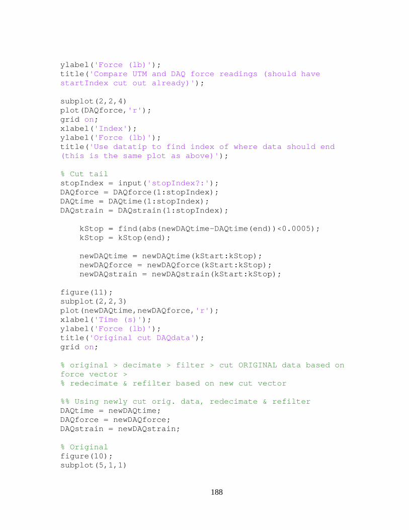
188

ylabel('Force (lb)'); title('Compare UTM and DAQ force readings (should have startIndex cut out already)'); subplot(2,2,4) plot(DAQforce,'r'); grid on; xlabel('Index'); ylabel('Force (lb)'); title('Use datatip to find index of where data should end (this is the same plot as above)'); % Cut tail stopIndex = input('stopIndex?:'); DAQforce = DAQforce(1:stopIndex); DAQtime = DAQtime(1:stopIndex); DAQstrain = DAQstrain(1:stopIndex); kStop = find(abs(newDAQtime-DAQtime(end))<0.0005); kStop = kStop(end); newDAQtime = newDAQtime(kStart:kStop); newDAQforce = newDAQforce(kStart:kStop); newDAQstrain = newDAQstrain(kStart:kStop); figure(11); subplot(2,2,3) plot(newDAQtime,newDAQforce,'r'); xlabel('Time (s)'); ylabel('Force (lb)'); title('Original cut DAQdata'); grid on; % original > decimate > filter > cut ORIGINAL data based on force vector > % redecimate & refilter based on new cut vector %% Using newly cut orig. data, redecimate & refilter DAQtime = newDAQtime; DAQforce = newDAQforce; DAQstrain = newDAQstrain; % Original figure(10); subplot(5,1,1)

189

plot(OrigDAQtime, OrigDAQstrain); xlabel('Time (s)') ylabel('Microstrain') title('Original DAQ data') grid on; subplot(5,1,2) plot(DAQtime,DAQstrain); xlabel('Time (s)') ylabel('Microstrain') title('Original (CUT) DAQ data') grid on; %% Decimate and filter to find index at which to cut original data % Decimate decimateBy = 400; % Each plateau is 803 pts long DAQforce = decimate(DAQforce,decimateBy); DAQforce = [0; DAQforce(2:end)]; % since sometimes the 1st point is super weird DAQtime = decimate(DAQtime,decimateBy); DAQstrain = decimate(DAQstrain,decimateBy); % DAQstrain = DAQstrain - DAQstrain(1); subplot(5,1,3) plot(DAQtime,DAQstrain); xlabel('Time (s)') ylabel('Microstrain') title('Decimated DAQ data') grid on; % Filter % Apply 9th order butterworth low-pass filter DAQstrain = filtfilt(b,a,DAQstrain); % DAQstrain = DAQstrain - DAQstrain(1); subplot(5,1,4) plot(DAQtime,DAQstrain); xlabel('Time (s)') ylabel('Microstrain') title('Filtered Decimated DAQ data') grid on; %% Shift

190

DAQforce = DAQforce - DAQforce(1); DAQtime = DAQtime - DAQtime(1); DAQstrain = DAQstrain - DAQstrain(1); subplot(5,1,5) plot(DAQtime,DAQstrain); xlabel('Time (s)') ylabel('Microstrain') title('Shifted Cut Filtered Decimated DAQ data') grid on; %% Check figure(12); plot(UTMtime,UTMforce,DAQtime,DAQforce,'r') legend('UTM','DAQ','Location','SouthEast'); title('Final DAQ data vs UTM'); xlabel('Time (s)'); ylabel('Force (lbs)'); grid on; %% Preview P-eps figure(13); plot(DAQstrain,DAQforce); xlabel('Microstrain'); ylabel('Force (lbs)'); grid on; title(['P-\epsilon relationship for ',inputname(1)]); %% Redefine daqnew = [DAQtime,DAQforce,DAQstrain]; end

191

Appendix D

Larger version of load-displacement and load-strain data with labels

192

193

Appendix E

Extraction and curve-fitting code for finding shape of generating curve

function [coeff] = fitGCoutline(filename,firstWhorlYRange) % Function that reads the BW image of a shell scan % and outputs the curve-fit simulation of the outline % Replaces aks.m and FRadius.m (my versions) % Used directly by surface3.m (my versions) % Has some issues with images: % - make sure input image is black/white only; no grayscale % - input shape needs to be reasonably round (no weird bumps) for below % code to work % - amount of white space is not important %% Read BW image pic = imread(filename); % 'string.type' pic = im2bw(pic,0.5); % convert to b/w image, 0.5 level is arbitrary (from matlab example) %% Convert BW image into x,y data % Note the different if-loops for image types (still not finalized-- see aks.m files) s = size(pic); % 1x2 vector, in number of pixels k = 1; for i = 1:s(1) % first element in size (number of rows) for j = 1:s(2) % number of columns in pic if pic(i,j) == 0; % for BW-only (logical) images; if black, % if pic(i,j) ~= 15; % for grayscale (uint8) images x(k) = j; % then record the index of black pixel y(k) = i; % x and y are vectors containing only information about black % pixels ("pixels with information") k = k + 1; end end

194

end y = -y; % it's upside down for some reason % Convert to mm (11.8 pixels/mm) x = x/11.8; y = y/11.8; % Attempt to scale down scalar = range(y)/firstWhorlYRange; x = x/scalar; % this is now the size of the first whorl y = y/scalar; manualScale = 1.5; x = x*manualScale; y = y*manualScale; figure; plot(x,y,'* r'); xlabel('x'); ylabel('y'); axis equal %% Convert x,y data into theta, R data % x,y data should represent the black outline only (no white data) % Find centroid & center image around centroid xo = mean(x); yo = mean(y); x = x - xo; y = y - yo; % Calculate R and theta using simple trigonometry R=(x.^2+y.^2).^0.5; % distance formula (1x216) for i=1:length(x) if y(i)>=0 th(i)=acos(x(i)/R(i)); % 0<=theta<=pi else th(i)=2*pi-acos(x(i)/R(i)); % pi<=theta<=2pi end end temp = size(th); if temp(1) < temp(2) % if a row vector

195

th = th'; end % Sort for plotting purposes V = [th R']; % [theta (lengthx1) | radius (lengthx1)] V = sortrows(V,1); % in order of theta % Rewrite in order th = V(:,1); R = V(:,2); % R = smooth(R,5); % default: 5-pt moving average -- user discretion %% Fit to Gaussian function % .' = nonconjugate array transpose f = fit(th,R,'gauss8'); % generate coefficients for curve fit figure; plot(f,th,R); % plot data with curve fit xlabel('theta (radians)'); ylabel('radius'); %% Extract Gaussian coefficients & recalcuate radius to represent the curve fit image % We need to do this since the imported image is a set of discrete points, % while the curve fit equation is continuous coeff = coeffvalues(f); % in order of a1, b1, c1, a2, b2, c2 ... c8 (1x24 vector) % Initialize set_a = []; set_b = []; set_c = []; thFit = linspace(0,2*pi,1000); % arbitrary; is a clean version of theta rFit = 0; for i = 1:length(coeff) if mod(i/3,1) == 0 % check if it is an integer; only continues in if-loop if true set_a = [set_a coeff(i-2)]; set_b = [set_b coeff(i-1)]; set_c = [set_c coeff(i)]; end

196

end % Gaussian function (see wiki) % is given as f(x) = a*exp(-((x-b)^2)/(2*c^2)); for i = 1:8 % gauss8 rFit = rFit + set_a(i)*exp(-((thFit-set_b(i))./set_c(i)).^2); end % Make sure the outline of GC is a closed, smooth loop % rFit(end) = (rFit(end)+rFit(1))/2; % rFit(1:100) = linspace(rFit(end),rFit(100),100); % rFit(end-99:end) = linspace(rFit(end-99),rFit(end),100); %% Calculate fitted x,y and plot xFit = rFit.*cos(thFit); yFit = rFit.*sin(thFit); figure; plot(x,y,'* r'); hold on; plot(xFit,yFit,'b'); xlabel('x in mm'); ylabel('y in mm'); axis equal title('Comparison of scanned outline to curvefit'); legend('Scanned outline','Curvefit'); end

197

Appendix F

Deleting overlapping nodes to tie sutures

%% Generate node & element vectors % This section replaces the one above that generates NodeMatrix, % ElemMatrix, and writes these to text files to import into ANSYS. This % improved section removes overlapping nodes and keeps all elements unique % -- this ensures that the "tip slice" is connected to the rest of the % shell in ANSYS because the elements are built from pre-existing nodes. NodeMatrix = nmg(X,Y,Z); % FROM ORIGINAL SURF (4x11175) sizeNM = size(NodeMatrix); % [numRows numCol] ElementsMatrix = emg(X); % (4x10704) NodeMatrix2 = nmg(Xi,Yi,Zi); % (4x216) NodeMatrix2(1,:) = NodeMatrix2(1,:) + sizeNM(2); % 1st row is the node num; node nums+numCol = start counting new nodes at the end of previous matrix ElementsMatrix2 = emg(Xi) + sizeNM(2); %% Delete overlapping nodes & refix elements to correct nodes % Delete overlapping nodes at body sutures & replace element boundaries % Checks to see if the difference between all nodes is negligible, and % replaces the later nodes with ones that have already appeared % Keeps record of which nodes are deleted, and replaces these values with % the new nodes in ElementsMatrix. These updated matrices are written to % file for output to ANSYS. sizeEM = size(ElementsMatrix); % foolproof way to get "length" for i = 1:sizeNM(2)-1

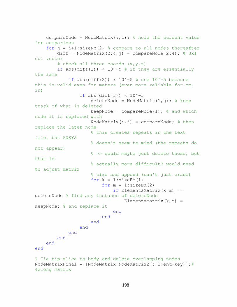
198

compareNode = NodeMatrix(:,i); % hold the current value for comparison for j = i+1:sizeNM(2) % compare to all nodes thereafter diff = NodeMatrix(2:4,j) - compareNode(2:4); % 3x1 col vector % check all three coords (x,y,z) if abs(diff(1)) < 10^-5 % if they are essentially the same if abs(diff(2)) < 10^-5 % use 10^-5 because this is valid even for meters (even more reliable for mm, in) if abs(diff(3)) < 10^-5 deleteNode = NodeMatrix(1,j); % keep track of what is deleted keepNode = compareNode(1); % and which node it is replaced with NodeMatrix(:,j) = compareNode; % then replace the later node % this creates repeats in the text file, but ANSYS % doesn't seem to mind (the repeats do not appear) % >> could maybe just delete these, but that is % actually more difficult? would need to adjust matrix % size and append (can't just erase) for k = 1:sizeEM(1) for m = 1:sizeEM(2) if ElementsMatrix(k,m) == deleteNode % find any instance of deleteNode ElementsMatrix(k,m) = keepNode; % and replace it end end end end end end end end % Tie tip-slice to body and delete overlapping nodes NodeMatrixFinal = [NodeMatrix NodeMatrix2(:,1:end-key)];% 4xlong matrix

199

% Replace the deleted overlappping nodes in tip-slice sizeEM2 = size(ElementsMatrix2); numRowEM2 = sizeEM2(1); numColEM2 = sizeEM2(2); % foolproof way to do "length" cutOff = NodeMatrix2(1,end-key); % this is the last non-overlapping node for i=1:numColEM2 for j=1:numRowEM2 if ElementsMatrix2(j,i) > cutOff ElementsMatrix2(j,i) = ElementsMatrix2(j,i) - cutOff; end end

200

Appendix G

Division of elements into sections with discretized thickness

function [ElementsMatrixSection,z_1,z_2,r,t_output] = divShellElements2(ElementsMatrix,X,NodeMatrixFinal,numWhorls) % Use pre-created ColumnElementsMatrix, then divide into sections % This function generates separate element matrices for each section that % has a different cross-sectional area per rigid link. % Also outputs the correct cross-sectional area for the rigid link in this % section. % Input: % numOfSections = number of sections to split up the lateral area of the columella's cone outline % Output: % ColumnElementsMatrixSection = a cell of matrices; each matrix contains % the nodes for one section sizeX = size(X); HSmatrix = []; % Rearrange ElementsMatrix to be the length of one HS for i = 1:sizeX(1)-1 HSset = ElementsMatrix(:,i*(sizeX(2)-1)-(sizeX(2)-1)+1:i*(sizeX(2)-1));%4x915 HSmatrix = [HSmatrix;HSset]; end % Then divide into sections sizeHSm = size(HSmatrix); sectionLength = sizeHSm(2)/numWhorls; % equal # of elem per whorl, may not be an integer numOfSections = ceil(numWhorls); for i = 1:numOfSections % if 19.75, then 20 sections EMSection = []; temp = [];

201

if i < numOfSections secLength = floor(sectionLength); for j = 1:sizeHSm(1)/4 temp = HSmatrix(j*4-3:j*4,i*secLength-secLength+1:i*secLength); EMSection = [EMSection,temp]; % append end else % when you reach the last section: beginLastSection = secLength*(numOfSections-1)+1; secLength = length(HSmatrix)-beginLastSection; % the last section will be the largest, since all the leftover % decimal values are tacked on at the end. The whorls from before % may be _slightly_ smaller than a full whorl. for j = 1:sizeHSm(1)/4 temp = HSmatrix(j*4-3:j*4,beginLastSection:beginLastSection+floor(secLength/4)); % the "last section" only captures 1/4 of the z-height EMSection = [EMSection,temp]; % append end end ElementsMatrixSection{i} = EMSection; % this is sorted by height, not by HS# end EMSection = []; temp = []; % Then append the last 3/4 of the last whorl as a new section for j = 1:sizeHSm(1)/4 temp = HSmatrix(j*4-3:j*4,beginLastSection+floor(secLength/4)+1:end); EMSection = [EMSection,temp]; % append end ElementsMatrixSection{numOfSections+1} = EMSection; %% Calculate the thickness for each section for i = 1:numOfSections firstNode = ElementsMatrixSection{i}(1,1); % lastNode = ElementsMatrixSection{i}(3,end);

202

lastNode = ElementsMatrixSection{i}(3,:); % 1xlong vector for j = 1:length(lastNode) zmap(j) = NodeMatrixFinal(4,lastNode(j)); xmap(j) = NodeMatrixFinal(2,lastNode(j)); end zmap = zmap'; [maxz,maxZind] = max(abs(zmap)); lastNode = ElementsMatrixSection{i}(3,maxZind); % this one works % Find maximum radius in this section xmap = xmap'; [maxx, maxXind] = max(abs(xmap)); rNode = ElementsMatrixSection{i}(3,maxXind); % using the 3rd row may not be the largest r, but it will be close rX = abs(NodeMatrixFinal(2,rNode)); rY = abs(NodeMatrixFinal(3,rNode)); r(i) = sqrt(rX^2+rY^2); z1 = abs(NodeMatrixFinal(4,firstNode)+0.2449); % coordinates z2 = abs(NodeMatrixFinal(4,lastNode)+0.2449); % shift to 0 t1 = 0.0024*z1+0.029; t2 = 0.0024*z2+0.029; t_output(i) = t1; % use thin end to see if this loosens the shell enough for validation z_1(i) = z1; %(z2-z1)*2/3+z1; z_2(i) = z2; % r_1(i) = r1; % r_2(i) = r2; % Note: t1 uses z1 to determine the thickness of the whole section, while % the vol. capacity and mass are determined by z2, the end of the section. end end

203

REFERENCES

ACI Committee 318. 2011. Building Code Requirements for Structural Concrete (ACI 318-11) and Commentary. American Concrete Institute. http://210.42.35.80/G2S/eWebEditor/uploadfile/20110806224616634.pdf.

Aizenberg, Joanna, James C Weaver, Monica S Thanawala, Vikram C Sundar, Daniel E Morse, and Peter Fratzl. 2005. “Skeleton of Euplectella Sp.: Structural Hierarchy from the Nanoscale to the Macroscale.” Science (New York, N.Y.) 309 (5732): 275–78. doi:10.1126/science.1112255.

Batty, Michael. 2013. The New Science of Cities. MIT Press. http://www.jstor.org/stable/j.ctt9qf7m6.

Benyus, Janine. n.d. “A Biomimicry Primer.” Biomimicry 3.8. http://biomimicry.net/b38files/A_Biomimicry_Primer_Janine_Benyus.pdf.

Bernett, Allison. 2015. “Biomimicry, Bioutilization, Biomorphism: The Opportunities of Bioinspired Design.” Blog. Terrapin Bright Green. January 17. http://www.terrapinbrightgreen.com/blog/2015/01/biomimicry-bioutilization-biomorphism/.

Bettencourt, Luís M. A., José Lobo, Dirk Helbing, Christian Kühnert, and Geoffrey B. West. 2007. “Growth, Innovation, Scaling, and the Pace of Life in Cities.” Proceedings of the National Academy of Sciences of the United States of America 104 (17): 7301–6. doi:10.1073/pnas.0610172104.

Bier, Henriette. 2014. “Robotic Building.” 2018. http://www.hyperbody.nl/research/projects/robotic-building/.

Biomimicry Institute. 2014. “Termite-Inspired Air Conditioning.” http://biomimicryinstitute.org/case-studies/case-studies/termite-inspired-air-conditioning.html.

———. n.d. “Nature’s Unifying Patterns: 10 Lessons to Consider Every Time You Design Something.” Biomimicry Institute. biomimicry.org.

Blanton, Patricia L., and Norman L. Biggs. 1968. “Density of Fresh and Embalmed Human Compact and Cancellous Bone.” American Journal of Physical Anthropology 29 (1): 39–44. doi:10.1002/ajpa.1330290113.

Bojovic, Marija. 2013. “Honeycomb Facade for Softer Urban Landscape / Sinosteel, Tianjin by MAD Architects.” Architecture Magazine. eVolo. March 26. http://www.evolo.us/architecture/honeycomb-facade-for-softer-urban-landscape-sinosteel-tianjin-by-mad-architects/.

Brand, Stewart. 1995. How Buildings Learn: What Happens after They’re Built. New York: Penguin Books.

Calvert Marine Museum. 2016. “Invertebrate Fossils | Calvert Marine Museum, MD - Official Website.” Accessed June 3. http://www.calvertmarinemuseum.com/336/Invertebrate-Fossils.

Cha, Philip D., and John I. Molinder. 2006. Fundamentals of Signals and Systems with CD-ROM: A Building Block Approach. Cambridge University Press.

204

Chamberlain, John A., Jr. 1978. “Mechanical Properties of Coral Skeleton: Compressive Strength and Its Adaptive Significance.” Paleobiology 4 (4): 419–35.

Chamberlain, John A., and Gerd E. G. Westermann. 1976. “Hydrodynamic Properties of Cephalopod Shell Ornament.” Paleobiology 2 (4): 316–31.

Chen, Diana A., Leidy E. Klotz, and Brandon E. Ross. 2016. “Mathematically Characterizing Natural Systems for Adaptable, Biomimetic Design.” Procedia Engineering, ICSDEC 2016 – Integrating Data Science, Construction and Sustainability, 145: 497–503. doi:10.1016/j.proeng.2016.04.031.

Chen, Diana A., Brandon E. Ross, and Leidy E. Klotz. 2014a. “Exploring Infrastructure Solutions through Bio-Inspired, Adaptable, Structural Art.” In ICSI 2014, 947–59. Long Beach, CA: American Society of Civil Engineers. http://ascelibrary.org/doi/abs/10.1061/9780784478745.089.

———. 2014b. “Lessons from a Coral Reef: Biomimicry for Structural Engineers.” Journal of Structural Engineering, December, 2514002. doi:10.1061/(ASCE)ST.1943-541X.0001216.

Chen, Diana, Kylie Tawney, and Brandon Ross. 2015. “GASTROPOD SHELLS: QUANTITATIVE BIOMIMICRY FOR ADAPTABLE STRUCTURES.” In . Pittsburgh, PA.

Chen, Po-Yu, Joanna McKittrick, and Marc André Meyers. 2012. “Biological Materials: Functional Adaptations and Bioinspired Designs.” Progress in Materials Science 57 (8): 1492–1704. doi:10.1016/j.pmatsci.2012.03.001.

Cohen, Steve, and Michael Graham Richard. 2006. “New York City: Sustainable City?” TreeHugger. October 19. http://www.treehugger.com/travel/new-york-city-sustainable-city.html.

Cortie, MB. 1989. “Models for Mollusc Shell Shape.” South African Journal of Science 85 (July): 454–60.

Cortie, Michael B., Katie E. McBean, and Margaret M. Elcombe. 2006. “Fracture Mechanics of Mollusc Shells.” Physica B: Condensed Matter, Proceedings of the Eighth International Conference on Neutron Scattering, 385–386, Part 1 (November): 545–47. doi:10.1016/j.physb.2006.05.356.

Creer, Brent Y., Captain Harald A. Smedal, USN (MC), and Rodney C. Wingrove. 1960. “Centrifuge Study of Pilot Tolerance to Acceleration and the Effects of Acceleration on Pilot Performance.” Technical Note D-337. Moffett Field, California: NASA Ames Research Center. http://ntrs.nasa.gov/archive/nasa/casi.ntrs.nasa.gov/19980223621.pdf.

Csete, Marie E., and John C. Doyle. 2002. “Reverse Engineering of Biological Complexity.” Science 295 (5560): 1664–69. doi:10.1126/science.1069981.

Curwood, Steve, and Anamarija Frankic. 2012. Living on Earth: Design Inspiration from NatureTranscript. http://www.loe.org/shows/segments.html?programID=12-P13-00046&segmentID=7.

Davidson, Marc S. 2009. “Towards an Understanding of the Role of Aragonite in the Mechanical Properties of Nacre.” SLAC-TN-10-005. Stanford, CA: Stanford Linear Accelerator Center.

205

“Design for Deconstruction.” 2010. X1-96912701. EPA Region 9. http://www.epa.gov/region9/greenbuilding/pdfs/DesignForDeconstrManual.pdf.

DTZ Consulting. 2000. “Demolition and New Building on Local Authority Estates.” U.K. Department of the Environment, Transport and the Regions.

Dunham-Jones, Ellen, and June Williamson. 2011. Retrofitting Suburbia: Urban Design Solutions for Redesigning Suburbs. Updated ed. Hoboken, N.J: Wiley.

Dym, Clive L., and Patrick Little. 2008. Engineering Design: A Project Based Introduction. 3 edition. Hoboken, N.J. : Chichester: Wiley.

Etherington, Rose. 2008. “Sinosteel International Plaza by MAD.” Dezeen Magazine. July 30. http://www.dezeen.com/2008/07/30/sinosteel-international-plaza-by-mad/.

Etter, Ron, Mark W. Denny, and Steven Dean Gaines. 2007. “Snails.” In Encyclopedia of Tidepools and Rocky Shores, 530–36. University of California Press.

Faghih Shojaei, M., V. Mohammadi, H. Rajabi, and A. Darvizeh. 2012. “Experimental Analysis and Numerical Modeling of Mollusk Shells as a Three Dimensional Integrated Volume.” Journal of the Mechanical Behavior of Biomedical Materials 16 (December): 38–54. doi:10.1016/j.jmbbm.2012.08.006.

Fazli, N., A. Abedian, H. Teimouri, and International Council of the Aeronautical Sciences. 2008. “Effects of Hierarchy Order on Natural Frequencies and Vibration Transmission of Self-Similar Trusses.” In ICAS PROCEEDINGS -CD-ROM EDITION-; 101 International Council of the Aeronautical Sciences; 8th AIAA Aviation Technology, Integration, and Operations (ATIO) International Congress; 26th, International Council of the Aeronautical Sciences; 8th AIAA Aviation Technology, Integration, and Operations (ATIO). Optimage ; International Council of the Aeronautical Sciences. http://www.icas.org/ICAS_ARCHIVE/ICAS2008/PAPERS/591.PDF.

Feifer, Jason. 2015. “The London Olympic Facilities Are Cleverly Designed To Outlast The Games.” Fast Company. Accessed May 6. http://www.fastcompany.com/1835673/london-olympic-facilities-are-cleverly-designed-outlast-games.

Fowler, Deborah R., Hans Meinhardt, and Przemyslaw Prusinkiewicz. 1992. “Modeling Seashells.” ACM SIGGRAPH Computer Graphics 26 (2): 379–87. doi:10.1145/142920.134096.

Fratzl, Peter. 2005. “Hierarchical Structure and Mechanical Adaptation of Biological Materials.” In Learning from Nature How to Design New Implantable Biomaterialsis: From Biomineralization Fundamentals to Biomimetic Materials and Processing Routes, edited by R. L. Reis and S. Weiner, 15–34. NATO Science Series II: Mathematics, Physics and Chemistry 171. Springer Netherlands. http://materialsknowledge.org/docs/Peter_Fratzl_lecture_notes.pdf.

———. 2007. “Biomimetic Materials Research: What Can We Really Learn from Nature’s Structural Materials?” Journal of The Royal Society Interface 4 (15): 637–42. doi:10.1098/rsif.2007.0218.

Fratzl, Peter, and Himadri S. Gupta. 2007. “Nanoscale Mechanisms of Bone Deformation and Fracture.” In Handbook of Biomineralization, edited by Edmund Bäuerlein,

206

397–414. Wiley-VCH Verlag GmbH. http://onlinelibrary.wiley.com/doi/10.1002/9783527619443.ch23/summary.

Hall, Kenneth, and Gerald Porterfield. 2001. Community By Design: New Urbanism for Suburbs and Small Communities. 1 edition. New York: McGraw-Hill Education.

Hardy, Eddie. 2016. “Turritella Terebra Terebra.” March 23. http://www.gastropods.com/5/Shell_255.shtml.

Heintz, Maggy. 2009. “Biomimicry to the Rescue.” Materials Today 12 (3): 6. Helms, Michael E., Swaroop S. Vattam, Ashok K. Goel, Jeannette Yen, and Marc

Weissburg. 2008. “Problem-Driven and Solution-Based Design: Twin Processes of Biologically Inspired Design.” In Proceedings of the 28th Annual Conference of the Association for Computer Aided Design in Architecture. Minneapolis, Minnesota: Association for Computer Aided Design in Architecture.

Hoerner, Sighard F. 1951. Aerodynamic Drag: Practical Data on Aerodynamic Drag Evaluated and Presented. Otterbein Press.

Horwitz-Bennett, Barbara. 2009. “Design Echoes Natural Life with the Science of Biomimicry,” February. http://www.interiorsandsources.com/article-details/articleid/6984/title/biomimicry-nature-s-lessons.aspx.

Hughes, Thomas P. 1987. “The Evolution of Large Technological Systems.” The Social Construction of Technological Systems: New Directions in the Sociology and History of Technology, 51–82.

Hutchinson, J.M.C. 1989. “Control of Gastropod Shell Shape; The Role of the Preceding Whorl.” Journal of Theoretical Biology 140 (4): 431–44. doi:10.1016/S0022-5193(89)80107-9.

Illert, C. 1989. “Formulation and Solution of the Classical Seashell Problem.” Il Nuovo Cimento D 11 (5): 761–80. doi:10.1007/BF02451562.

Jackson, A. P., J. F. V. Vincent, and R. M. Turner. 1988. “The Mechanical Design of Nacre.” Proceedings of the Royal Society of London B: Biological Sciences 234 (1277): 415–40. doi:10.1098/rspb.1988.0056.

Jirapong, Kamon, and Robert J. Krawczyk. 2003. “Case Study: Modeling the Interior Structure of Seashells.” In . University of Granada in Spain. http://mypages.iit.edu/~krawczyk/shell01/kj01.pdf.

Kennedy, B., A. Buikema, and J.K.S. Nagel. 2015. “Integrating Biology, Design, and Engineering for Sustainable Innovation.” In 2015 IEEE Integrated STEM Education Conference (ISEC), 88–93. doi:10.1109/ISECon.2015.7119952.

Kestner, Dirk M., Jennifer Goupil, and Emily Lorenz. 2010. Sustainability Guidelines for the Structural Engineer. ASCE Publications.

Knippers, Jan, and Thomas Speck. 2012. “Design and Construction Principles in Nature and Architecture.” Bioinspiration & Biomimetics 7 (1): 15002. doi:10.1088/1748-3182/7/1/015002.

Kohler, Niklaus, Holger König, Johannes Kreissig, and Thomas Lützkendorf. 2010. A Life Cycle Approach to Buildings: Principles - Calculations - Design Tools. Walter de Gruyter.

207

Kunkel, Catherine M., Robert W. Hallberg, and Michael Oppenheimer. 2006. “Coral Reefs Reduce Tsunami Impact in Model Simulations.” Geophysical Research Letters 33 (23): L23612. doi:10.1029/2006GL027892.

Kupfer, Helmut, Hubert K. Hilsdorf, and Hubert Rusch. 1969. “Behavior of Concrete Under Biaxial Stresses.” Journal Proceedings 66 (8): 656–66.

Lakes, Roderic. 1993. “Materials with Structural Hierarchy.” Nature 361 (6412): 511–15. doi:10.1038/361511a0.

Langston, Craig. 2008. “The Sustainability Implications of Building Adaptive Reuse.” In . Beijing, China. http://works.bepress.com/cgi/viewcontent.cgi?article=1000&context=craig_langston.

Lemer, A. 1996. “Infrastructure Obsolescence and Design Service Life.” Journal of Infrastructure Systems 2 (4): 153–61.

Lienhard, J, S Schleicher, S Poppinga, T Masselter, M Milwich, T Speck, and J Knippers. 2011. “Flectofin: A Hingeless Flapping Mechanism Inspired by Nature.” Bioinspiration & Biomimetics 6 (4): 45001. doi:10.1088/1748-3182/6/4/045001.

Linsley, Robert M. 1977. “Some ‘Laws’ of Gastropod Shell Form.” Paleobiology 3 (2): 196–206.

———. 1978. “Locomotion Rates and Shell Form in the Gastropoda.” Malacologia 17 (2): 193–206.

“London 2012 - Olympic Stadium.” 2014. Architecture. Detail.de. April 29. http://www.detail-online.com/architecture/topics/london-2012-olympic-stadium-019389.html.

Luz, Gisela M., and João F. Mano. 2009. “Biomimetic Design of Materials and Biomaterials Inspired by the Structure of Nacre.” Philosophical Transactions of the Royal Society of London A: Mathematical, Physical and Engineering Sciences 367 (1893): 1587–1605. doi:10.1098/rsta.2009.0007.

Madin, J. S., A. I. Dell, E. M. P. Madin, and M. C. Nash. 2012. “Spatial Variation in Mechanical Properties of Coral Reef Substrate and Implications for Coral Colony Integrity.” Coral Reefs 32 (1): 173–79. doi:10.1007/s00338-012-0958-0.

Madin, Joshua S. 2005. “Mechanical Limitations of Reef Corals during Hydrodynamic Disturbances.” Coral Reefs 24 (4): 630–35. doi:10.1007/s00338-005-0042-0.

Magazines, Hearst. 1981. Popular Mechanics. Hearst Magazines. Mallach, Alan. 2006. Bringing Buildings Back: From Abandoned Properties to Community

Assets : A Guidebook for Policymakers and Practitioners. Rutgers University Press.

“Mathematical Study of Mollusk Shells.” 2015. American Mathematical Society. Accessed January 8. http://www.ams.org/samplings/feature-column/fcarc-shell5.

Meyers, Marc André, Po-Yu Chen, Albert Yu-Min Lin, and Yasuaki Seki. 2008. “Biological Materials: Structure and Mechanical Properties.” Progress in Materials Science 53 (1): 1–206. doi:10.1016/j.pmatsci.2007.05.002.

“Minnesota Demolition Survey: Phase Two Report, Prepared for: Forintek Canada Corp.” 2004. The Athena Institute. http://briscoman.com/sites/default/files/Athena_Demolition_Survey.pdf.

208

Moseley, H. 1838. “On the Geometrical Forms of Turbinated and Discoid Shells.” Philosophical Transactions of the Royal Society of London 128 (January): 351–70.

Mumford, Lewis. 1961. The City in History: Its Origins, Its Transformations, and Its Prospects. Houghton Mifflin Harcourt.

National Research Council, Committee on Key Challenge Areas for Convergence and Health, Board on Life Sciences, and Division on Earth and Life Studies. 2014. Convergence: Facilitating Transdisciplinary Integration of Life Sciences, Physical Sciences, Engineering, and Beyond. Washington, D.C.: The National Academies Press. http://www.nap.edu/openbook.php?record_id=18722&page=1.

Neves, N. M., and J. F. Mano. 2005. “Structure/mechanical Behavior Relationships in Crossed-Lamellar Sea Shells.” Materials Science and Engineering: C, NATO Advanced Study Institute (ASI on Learning from Nature How to design New Implantable Biomaterials: From Biomineralization Fundamentals to Biomimetic Materials and Processing Routes) NATO Advanced Study Institute (ASI on Learning from Nature How to design New Implantable Biomaterials: From Biomineralization Fundamentals to Biomimetic Materials and Processing Routes), 25 (2): 113–18. doi:10.1016/j.msec.2005.01.004.

Newman, M. E. J. 2011. “Complex Systems: A Survey.” American Journal of Physics 79 (8): 800. doi:10.1119/1.3590372.

Oda, Juhachi, Jiro Sakamoto, and Kenichi Sakano. 2006. “Mechanical Evaluation of the Skeletal Structure and Tissue of the Woodpecker and Its Shock Absorbing System.” JSME International Journal Series A Solid Mechanics and Material Engineering 49 (3): 390–96. doi:10.1299/jsmea.49.390.

Palmer, A. Richard. 1980. “Locomotion Rates and Shell Form in the Gastropoda: A Re-Evaluation.” Malacologia 19 (2): 289–96.

Rajabi, H., A. Darvizeh, A. Shafiei, Sh. Eshghi, and A. Khaheshi. 2014. “Experimental and Numerical Investigations of Otala Lactea’s shell–I. Quasi-Static Analysis.” Journal of the Mechanical Behavior of Biomedical Materials 32 (April): 8–16. doi:10.1016/j.jmbbm.2013.12.008.

Ratnieks, Francis L. W. 2008. “Biomimicry: Further Insights from Ant Colonies?” In Bio-Inspired Computing and Communication, edited by Pietro Liò, Eiko Yoneki, Jon Crowcroft, and Dinesh C. Verma, 58–66. Lecture Notes in Computer Science 5151. Springer Berlin Heidelberg. http://link.springer.com/chapter/10.1007/978-3-540-92191-2_6.

Raup, David M. 1961. “The Geometry of Coiling in Gastropods.” In Proceedings of the National Academy of Sciences of the United States of America, 47:602–9. 4. National Academy of Sciences. http://www.jstor.org/stable/70669?origin=JSTOR-pdf&seq=1#page_scan_tab_contents.

Reap, John, Dayna Baumeister, and Bert Bras. 2005. “Holism, Biomimicry and Sustainable Engineering.” In , 2005:423–31. ASME. doi:10.1115/IMECE2005-81343.

Reilly, D. T., and A. H. Burstein. 1975. “The Elastic and Ultimate Properties of Compact Bone Tissue.” Journal of Biomechanics 8 (6): 393–405.

209

Richard Barras, and Paul Clark. 1996. “Obsolescence and Performance in the Central London Office Market.” Journal of Property Valuation and Investment 14 (4): 63–78. doi:10.1108/14635789610153470.

Rosales, Ava B. 2002. “Snail Susceptibility to Crab Predation: A Case Study of Co-Evolution from Lake TAnganyika, East Africa.” http://www.geo.arizona.edu/nyanza/pdf/Rosales.pdf.

Rosati, Jean Dean. 1990. “Functional Design of Breakwaters for Shore Protection: Empirical Methods.” Final Technical Report CERC-90-15. Coastal Engineering Research Center, Department of the Army. Civil Works Research Work Unit 32535. http://www.dtic.mil/dtic/tr/fulltext/u2/a228024.pdf.

Ross, Brandon E., Diana A. Chen, Sheila Conejos, and Amin Khademi. 2016. “Enabling Adaptable Buildings: Results of a Preliminary Expert Survey.” Procedia Engineering, ICSDEC 2016 – Integrating Data Science, Construction and Sustainability, 145: 420–27. doi:10.1016/j.proeng.2016.04.009.

Saha, Sujoy Kumar, and Gian Piero Celata. 2011. “Advances in Modelling of Biomimetic Fluid Flow at Different Scales.” Nanoscale Research Letters 6 (1): 1–11. doi:10.1186/1556-276X-6-344.

Sarja, Asko. 2005. “Generic Limit State Design of Structures.” In . Lyon, France. http://www.irbnet.de/daten/iconda/06059017606.pdf.

Signor, Philip W. 1982. “Resolution of Life Habits Using Multiple Morphologic Criteria: Shell Form and Life-Mode in Turritelliform Gastropods.” Paleobiology 8 (4): 378–88.

Sorguç, Arzu Gönenç, and Semra Arslan Selçuk. 2013. “Computational Models in Architecture: Understanding Multi-Dimensionality and Mapping.” Nexus Network Journal 15 (2): 349–62. doi:10.1007/s00004-013-0150-z.

Tan, Ria. 2008. “Turritella Snails (Turritella Terebra) on the Shores of Singapore.” http://www.wildsingapore.com/wildfacts/mollusca/gastropoda/turritellidae/turritella.htm.

Thompson, D’Arcy Wentworth. 1945. On Growth and Form. Cambridge : University Press ; New York : Macmillan. http://archive.org/details/ongrowthform00thom.

Tietjens, O. G. 1934. Applied Hydro- and Aeromechanics. 1sted. New York: McGraw-Hill Book Company, Inc.

Timoshenko, Stephen, and S. Woinowsky-Krieger. 1959. Theory of Plates and Shells. McGraw-Hill.

Turner, Charles H., Stephen C. Cowin, Jae Young Rho, Richard B. Ashman, and Janet C. Rice. 1990. “The Fabric Dependence of the Orthotropic Elastic Constants of Cancellous Bone.” Journal of Biomechanics 23 (6): 549–61. doi:10.1016/0021-9290(90)90048-8.

US Department of Commerce, National Oceanic and Atmospheric Administration. 2012. “NOAA’s Coral Reef Information System (CoRIS) - What Are Coral Reefs.” February. http://www.coris.noaa.gov/about/what_are/.

US Geological Survey, Pacific Coastal & Marine Science Center. 2008. “Life of a Tsunami.” Tsunamis & Earthquakes. October 22. http://walrus.wr.usgs.gov/tsunami/basics.html.

210

Vincent, Julian F.V., Olga Bogatyreva, Anja-Karina Pahl, Nikolay Bogatyrev, and Adrian Bowyer. 2005. “Putting Biology into TRIZ: A Database of Biological Effects.” Creativity and Innovation Management 14 (1): 66–72. doi:10.1111/j.1476-8691.2005.00326.x.

Wang, Lizhen, Jason Tak-Man Cheung, Fang Pu, Deyu Li, Ming Zhang, and Yubo Fan. 2011. “Why Do Woodpeckers Resist Head Impact Injury: A Biomechanical Investigation.” PLoS ONE 6 (10): e26490. doi:10.1371/journal.pone.0026490.

Webster, Mark D. 2007. “Structural Design for Adaptability and Deconstruction: A Strategy for Closing the Materials Loop and Increasing Building Value.” In , 1–6. American Society of Civil Engineers. doi:10.1061/40946(248)27.

Whitacre, James M., and Axel Bender. 2013. “Pervasive Flexibility in Living Technologies Through Degeneracy-Based Design.” Artif. Life 19 (3_4): 365–386. doi:10.1162/ARTL_a_00116.

Whitenack, Lisa B., and Gregory S. Herbert. 2015. “Did Shell-Crushing Crabs Trigger an Escalatory Arms Race in the Aftermath of a Late Neogene Regional Mass Extinction Event? An Experimental Test.” Palaeogeography, Palaeoclimatology, Palaeoecology 417 (January): 57–65. doi:10.1016/j.palaeo.2014.09.026.

Wilkinson, Sara J. 2011. “The Relationship between Building Adaptation and Property Atrributes.” Victoria, Australia: Deakin University. http://dro.deakin.edu.au/eserv/DU:30036710/wilkinson-relationshipbetween-2011.pdf.

Wilkinson, Sara J., Hilde Remøy, and Craig Langston. 2014. Sustainable Building Adaptation: Innovations in Decision-Making. John Wiley & Sons.

Woesz, Alexander, James C. Weaver, Murat Kazanci, Yannicke Dauphin, Joanna Aizenberg, Daniel E. Morse, and Peter Fratzl. 2011. “Micromechanical Properties of Biological Silica in Skeletons of Deep-Sea Sponges.” Journal of Materials Research 21 (8): 2068–78. doi:10.1557/jmr.2006.0251.

Yashiro, T, T Kato, T Yoshida, and Y Komatsu. 1990. “Survey on Real Life Sapn of Office Buildings in Japan.” In , 215–26.

Yoon, Sang-Hee, and Sungmin Park. 2011. “A Mechanical Analysis of Woodpecker Drumming and Its Application to Shock-Absorbing Systems.” Bioinspiration & Biomimetics 6 (1): 16003. doi:10.1088/1748-3182/6/1/016003.

Zhang, Ge. 2012. “Biomimicry in Biomedical Research.” Organogenesis 8 (4): 101–2. doi:10.4161/org.23395.

Zhu, ZhaoDan, Wei Zhang, and ChengWei Wu. 2014. “Energy Conversion in Woodpecker on Successive Peckings and Its Role on Anti-Shock Protection of Brain.” Science China Technological Sciences 57 (7): 1269–75. doi:10.1007/s11431-014-5582-5.