The Accuracy of Perturbation Methods to Solve Small … · 2011-11-22 · The Accuracy of...
37
Transcript of The Accuracy of Perturbation Methods to Solve Small … · 2011-11-22 · The Accuracy of...


ISSN 1518-3548 CGC 00.038.166/0001-05
Working Paper Series Brasília n. 262 Nov. 2011 p. 1-36

Working Paper Series Edited by Research Department (Depep) – E-mail: [email protected] Editor: Benjamin Miranda Tabak – E-mail: [email protected] Editorial Assistant: Jane Sofia Moita – E-mail: [email protected] Head of Research Department: Adriana Soares Sales – E-mail: [email protected] The Banco Central do Brasil Working Papers are all evaluated in double blind referee process. Reproduction is permitted only if source is stated as follows: Working Paper n. 262. Authorized by Carlos Hamilton Vasconcelos Araújo, Deputy Governor for Economic Policy. General Control of Publications Banco Central do Brasil
Secre/Comun/Cogiv
SBS – Quadra 3 – Bloco B – Edifício-Sede – 1º andar
Caixa Postal 8.670
70074-900 Brasília – DF – Brazil
Phones: +55 (61) 3414-3710 and 3414-3565
Fax: +55 (61) 3414-3626
E-mail: [email protected]
The views expressed in this work are those of the authors and do not necessarily reflect those of the Banco Central or its members. Although these Working Papers often represent preliminary work, citation of source is required when used or reproduced. As opiniões expressas neste trabalho são exclusivamente do(s) autor(es) e não refletem, necessariamente, a visão do Banco Central do Brasil. Ainda que este artigo represente trabalho preliminar, é requerida a citação da fonte, mesmo quando reproduzido parcialmente. Consumer Complaints and Public Enquiries Center Banco Central do Brasil
Secre/Surel/Diate
SBS – Quadra 3 – Bloco B – Edifício-Sede – 2º subsolo
70074-900 Brasília – DF – Brazil
Fax: +55 (61) 3414-2553
Internet: <http://www.bcb.gov.br/?english>
The Accuracy of Perturbation Methods to Solve Small Open
Economy Models
Angelo M. Fasolo�
The Working Papers should not be reported as representing
the views of the Banco Central do Brasil. The views expressed in
the papers are those of the author and do not necessarily
re�ect those of the Banco Central do Brasil.
Abstract
This paper presents the evaluation of the canonical RBC models for small-open economies de-
scribed in Schmitt-Grohé and Uribe (2003) when its solution is obtained by perturbation methods up
to a third-order approximation. The models are evaluated in terms of accuracy of solution, ergodic
moments, and local responses in extreme regions of the state vector. Results show that the gains
from non-linear solutions are signi�cant in terms of accuracy and with respect to the outcome of
simulations: when compared to the linear approximation of the equilibrium conditions, non-linear
solution generates very di¤erent dynamics of the stationary-inducing devices and smaller responses
of consumption and output if the economy is in a state of low capital, both results highly dependent
on the assumptions regarding preferences. However, signi�cant changes in the main allocations of
the economy when using di¤erent solutions appear only when GHH preferences are abandoned.
JEL Codes: C63, C68, E37, F41
Keywords: Small open economy; Stationarity; Perturbation methods; Non-linear Solutions
�Research Department, Banco Central do Brasil. The author is thankful for the comments of Juan Rubio-Ramírez andan anonymous referee, as well as the participants of seminars at Banco Central do Brasil and Universidade Católica deBrasília. Remaining errors are entirely due to author�s fault. E-mail: [email protected]
3
1 Introduction
This paper evaluates the properties of the solutions generated by perturbation methods (�rst, second
and third-order approximations of the equilibrium conditions) of the basic RBC models for small open
economies described in Schmitt-Grohé and Uribe (2003)[21] �SGU (2003), henceforth. The solutions
are evaluated in terms of accuracy, ergodic moments and local responses in extreme regions of the state
variables describing the economy. The ergodic moments do not provide a complete picture of the models�
dynamic, and given the use of alternative calibrations and non-linear solutions, it is worth to explore
the properties of the basic RBC model for small open economies in situations of crisis, like a low level of
capital stock. The analysis becomes even more important considering the evidence presented in Seoane
(2011)[22], where the same models calibrated with parameters for Mexico do not provide equivalent
responses as the log-linear solution in SGU (2003)[21] does.
The inclusion of high-order approximations in the analysis is justi�ed by its increasing importance in
research on asset pricing and DSGE models for small open economies (SOE�s), especially the so-called
Emerging Economies. As an example, Collard and Juillard (2001)[7] work with a very simple asset
pricing model with a closed form representation in order to compare the properties of solutions based
on perturbation methods of di¤erent orders. The authors �nd that the gains of solving the model with
second and fourth-order approximations are signi�cant, especially when the growth rate of dividends is
very volatile or persistent over time. Recently, asset pricing models based on Epstein-Zin�s (1989)[8]
recursive preferences have been solved using perturbation methods, after Caldara, Fernández-Villaverde,
Rubio-Ramírez and Yao (2009)[6] show the good accuracy of high-order approximation of DSGE models
with these preferences. Examples of the solution of asset pricing models with recursive preferences using
perturbation methods are Aldrich and Kung (2009)[3] and Malkhozov and Shamloo (2010)[23].
In terms of DSGE models, non-linear approximations have recently seen its use increased for estima-
tion purposes, as these approximations allow the estimation of models with highly non-linear, non-Normal
structure of shocks. There is evidence that non-linear solutions applied to DSGE models with Normal
disturbances allow better identi�cation of structural parameters1 . High-order approximations are also
used to correctly express the main features of a non-linear, non-Gaussian structure of a model. As an ex-
ample combining all these features, Fernández-Villaverde, Guerrón-Quintana, Rubio-Ramírez and Uribe
(2009)[9] solve a model with portfolio adjustment costs after adding time-varying volatility processes for
the exogenous shocks. The use of a third-order perturbation is necessary, in this case, in order to capture
the e¤ect of changes in the process of volatility, as solutions based on low order approximations eliminate
those e¤ects.
In this paper, the most simple formulations of RBC models for SOE�s are evaluated under di¤erent
parameterization and di¤erent speci�cations for the utility function. The evaluation is based not only on
the computation of ergodic moments and impulse response functions, like in SGU (2003)[21] and Seoane
(2011)[22], but also on the accuracy of non-linear solutions and on how the model�s dynamics changes
once these non-linearities are incorporated in the solution. Simple models allow a clear understanding of
the transmission mechanism of shocks without compromising the �tting of business cycle moments. For
two main reasons, the initial simulations are based on Greenwood, Hercowitz and Hu¤man (1988)[12]
utility function (GHH): �rst, it is the same utility function used in SGU (2003)[21] and Seoane (2011)[22],
making the analysis here comparable with the literature; second, as GHH utility sets that labor supply
is not a function of consumption level in the intratemporal Euler equation, the latter adoption of a
conventional utility function allows the evaluation of the use of perturbation methods once wealth e¤ects
plays a signi�cant role in labor supply.
Results show that the calibration proposed in SGU (2003)[21] for developed economies is invariant,
1See An (2008)[4] and Fernández-Villaverde and Rubio-Ramírez (2005)[10].
4

in terms of ergodic moments, up to second and third-order approximations, delivering equivalent results
across models under GHH preferences. Ergodic moments are also invariant to reasonable increases in the
volatility of the economy, given GHH preferences. However, the local analysis of the state space shows
that di¤erent stationarity-inducing mechanism presents di¤erent dynamics when the model is solved
using non-linear methods. More speci�cally, the use of high-order approximations to solve the "debt-
elastic interest rate" model results in more volatile risk premium under GHH preferences. Simulations
also show that, even in a model without signi�cant real or nominal frictions, the impact of shocks over
consumption and output are smaller when the economy is in an initial state of low capital. From the
perspective of accuracy, the increase in volatility justi�es the use of high-order approximation of the
model, as the quality of the linear solution quickly deteriorates as the volatility of the economy increases.
The paper is organized as follows. The next section brie�y presents the four SOE�s RBC models used
in SGU (2003)[21], focusing on the description of the mechanisms to make the current account stationary.
Section 3 describes how to solve a model using perturbation methods and the procedures to simulate and
evaluate accuracy in these models. It also describes the initial two sets of parameters used in sections 4
and 5. Section 4 shows the results of the baseline calibration, while section 5 explores the consequences
of an increase in the economy�s volatility, based on a new calibration for Emerging Economies. Section
6 departs from the use of GHH preferences, while trying to match the same set of moments from the
calibration of section 5. Section 7 concludes.
2 The Model
The four variations of the model proposed in SGU (2003)[21] can be derived as an special case of the
general formulation described below. This presentation follows exactly the same notation as the authors.
In the general case, there is a large population of identical agents with the same period utility function,
U (ct; ht) : These agents solve the following problem:
maxE01Pt=0
�tU (ct; ht)
s:t: : �t+1 = ��ct; ht;ect;eht� �t; t � 0; �0 = 1
dt = (1 + rt�1) dt�1 � yt + ct + it +�(kt+1 � kt) + 32
�dt � d
�2yt = AtF (kt; ht)
kt+1 = it + (1� �) ktrt = r + 2
hexp
�edt � d�� 1ilogAt+1 = � logAt + �t+1; �t+1 � NIID
�0; �2�
�limj!1
Etdt+j
jQs=1
(1+rs)
� 0
In the problem, ect; eht; and edt are the aggregate levels of consumption, hours worked and foreigndebt, while d is the steady state level of debt. The �rst-order conditions of the model are taken in terms
of individual consumption, ct; hours worked, ht; capital, kt+1; foreign debt, dt; and the discount factor,
�t: The functional forms for U (c; h) ; � (c; h) ; � (kt+1 � kt) and F (k; h) completes the description of themodel. Those are given by:
U (c; h) =
�c� !�1h!
�1� � 11�
� (c; h) =�1 + c� !�1h!
�� 1F (k; h) = k�h1��
5
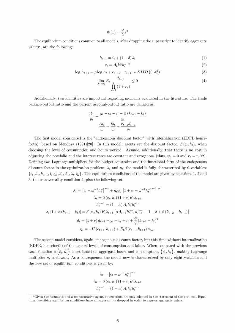
� (x) =�
2x2
The equilibrium conditions common to all models, after dropping the superscript to identify aggregate
values2 , are the following:
kt+1 = it + (1� �) kt (1)
yt = Atk�t h
1��t (2)
logAt+1 = � logAt + �t+1; �t+1 � NIID�0; �2�
�(3)
limj!1
Etdt+j
jQs=1
(1 + rs)
� 0 (4)
Additionally, two identities are important regarding moments evaluated in the literature. The trade
balance-output ratio and the current account-output ratio are de�ned as:
tbtyt=yt � ct � it � � (kt+1 � kt)
ytcatyt=tbtyt� rt�1dt�1
yt
The �rst model considered is the "endogenous discount factor" with internalization (EDFI, hence-
forth), based on Mendoza (1991)[20]. In this model, agents set the discount factor, � (ct; ht), when
choosing the level of consumption and hours worked. Assume, additionally, that there is no cost in
adjusting the portfolio and the interest rates are constant and exogenous (thus, 3 = 0 and rt = r; 8t).De�ning two Lagrange multipliers for the budget constraint and the functional form of the endogenous
discount factor in the optimization problem, �t and �t; the model is fully characterized by 9 variables:
fct; ht; kt+1; it; yt; dt; At; �t; �tg : The equilibrium conditions of the model are given by equations 1, 2 and3, the transversality condition 4, plus the following set:
�t =�ct � !�1h!t
�� + �t 1
�1 + ct � !�1h!t
�� 1�1�t = � (ct; ht) (1 + r)Et�t+1
h!�1t = (1� �)Atk�t h��t�t [1 + � (kt+1 � kt)] = � (ct; ht)Et�t+1
��At+1k
��1t+1 h
1��t+1 + 1� � + � (kt+2 � kt+1)
�dt = (1 + r) dt�1 � yt + ct + it +
�
2(kt+1 � kt)2
�t = �U (ct+1; ht+1) + Et� (ct+1; ht+1) �t+1
The second model considers, again, endogenous discount factor, but this time without internalization
(EDFE, henceforth) of the agents�levels of consumption and labor. When compared with the previous
case, function ��ect;eht� is set based on aggregate hours and consumption, �ect;eht� ; making Lagrange
multiplier �t irrelevant. As a consequence, the model now is characterized by only eight variables and
the new set of equilibrium conditions is given by:
�t =�ct � !�1h!t
�� �t = � (ct; ht) (1 + r)Et�t+1
h!�1t = (1� �)Atk�t h��t2Given the assumption of a representative agent, superscripts are only adopted in the statement of the problem. Equa-
tions describing equilibrium conditions have all superscripts dropped in order to express aggregate values.
6
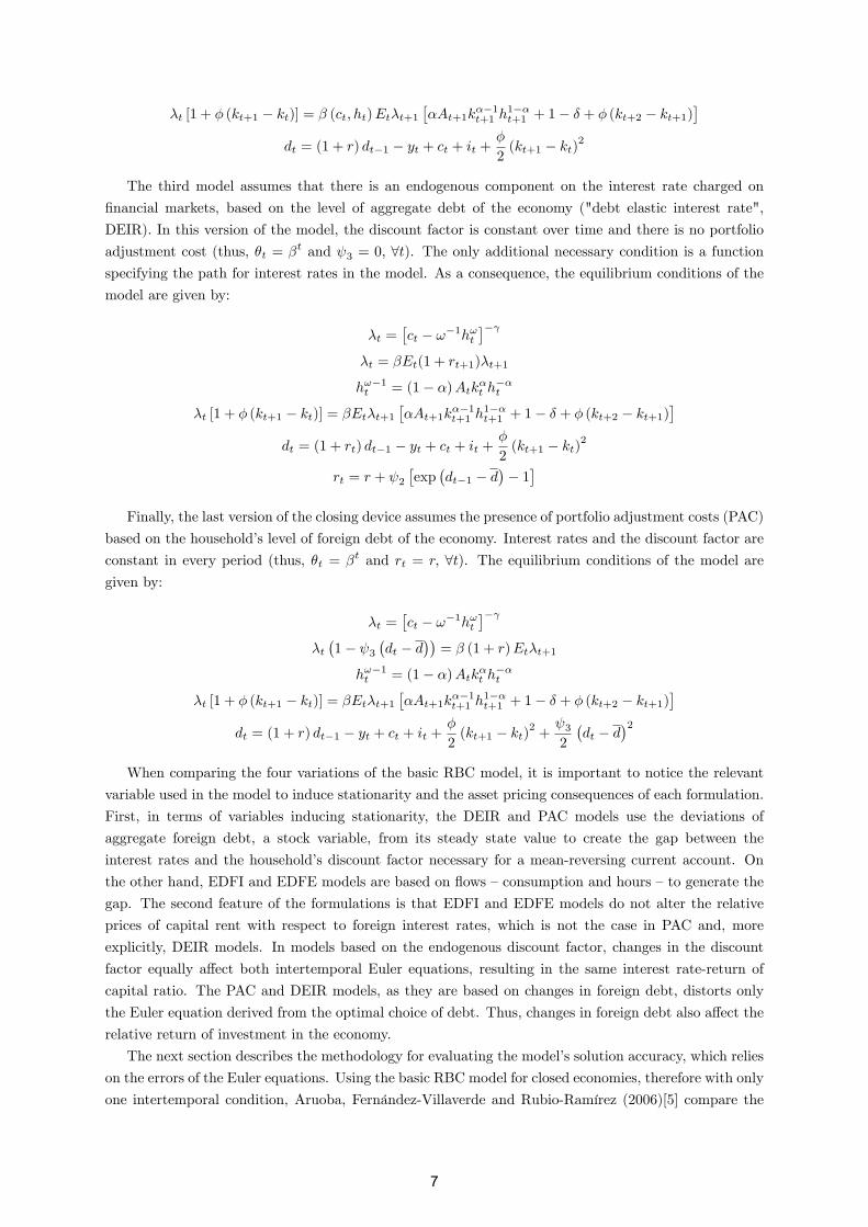
�t [1 + � (kt+1 � kt)] = � (ct; ht)Et�t+1��At+1k
��1t+1 h
1��t+1 + 1� � + � (kt+2 � kt+1)
�dt = (1 + r) dt�1 � yt + ct + it +
�
2(kt+1 � kt)2
The third model assumes that there is an endogenous component on the interest rate charged on
�nancial markets, based on the level of aggregate debt of the economy ("debt elastic interest rate",
DEIR). In this version of the model, the discount factor is constant over time and there is no portfolio
adjustment cost (thus, �t = �t and 3 = 0; 8t). The only additional necessary condition is a functionspecifying the path for interest rates in the model. As a consequence, the equilibrium conditions of the
model are given by:
�t =�ct � !�1h!t
�� �t = �Et(1 + rt+1)�t+1
h!�1t = (1� �)Atk�t h��t�t [1 + � (kt+1 � kt)] = �Et�t+1
��At+1k
��1t+1 h
1��t+1 + 1� � + � (kt+2 � kt+1)
�dt = (1 + rt) dt�1 � yt + ct + it +
�
2(kt+1 � kt)2
rt = r + 2�exp
�dt�1 � d
�� 1�
Finally, the last version of the closing device assumes the presence of portfolio adjustment costs (PAC)
based on the household�s level of foreign debt of the economy. Interest rates and the discount factor are
constant in every period (thus, �t = �t and rt = r; 8t). The equilibrium conditions of the model are
given by:
�t =�ct � !�1h!t
�� �t�1� 3
�dt � d
��= � (1 + r)Et�t+1
h!�1t = (1� �)Atk�t h��t�t [1 + � (kt+1 � kt)] = �Et�t+1
��At+1k
��1t+1 h
1��t+1 + 1� � + � (kt+2 � kt+1)
�dt = (1 + r) dt�1 � yt + ct + it +
�
2(kt+1 � kt)2 +
32
�dt � d
�2When comparing the four variations of the basic RBC model, it is important to notice the relevant
variable used in the model to induce stationarity and the asset pricing consequences of each formulation.
First, in terms of variables inducing stationarity, the DEIR and PAC models use the deviations of
aggregate foreign debt, a stock variable, from its steady state value to create the gap between the
interest rates and the household�s discount factor necessary for a mean-reversing current account. On
the other hand, EDFI and EDFE models are based on �ows �consumption and hours �to generate the
gap. The second feature of the formulations is that EDFI and EDFE models do not alter the relative
prices of capital rent with respect to foreign interest rates, which is not the case in PAC and, more
explicitly, DEIR models. In models based on the endogenous discount factor, changes in the discount
factor equally a¤ect both intertemporal Euler equations, resulting in the same interest rate-return of
capital ratio. The PAC and DEIR models, as they are based on changes in foreign debt, distorts only
the Euler equation derived from the optimal choice of debt. Thus, changes in foreign debt also a¤ect the
relative return of investment in the economy.
The next section describes the methodology for evaluating the model�s solution accuracy, which relies
on the errors of the Euler equations. Using the basic RBC model for closed economies, therefore with only
one intertemporal condition, Aruoba, Fernández-Villaverde and Rubio-Ramírez (2006)[5] compare the
7
accuracy of local and global solution methods using the Euler equation errors derived from the equilibrium
conditions on capital. Lim and McNelis (2008)[19] report accuracy tests based on the intertemporal
conditions of both capital and foreign bonds. However, Lim and McNelis (2008)[19] use only one of
the devices to induce stationarity, turning the error derived from the capital Euler equation as the only
comparable measure with this work. None of these papers consider the accuracy of perturbation methods
applied to the most simple RBC model for SOE�s.
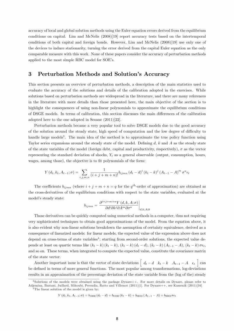
3 Perturbation Methods and Solution�s Accuracy
This section presents an overview of perturbation methods, a description of the main statistics used to
evaluate the accuracy of the solutions and details of the calibration adopted in the exercises. While
solutions based on perturbation methods are widespread in the literature, and there are many references
in the literature with more details than those presented here, the main objective of the section is to
highlight the consequences of using non-linear polynomials to approximate the equilibrium conditions
of DSGE models. In terms of calibration, this section discusses the main di¤erences of the calibration
adopted here to the one adopted in Seoane (2011)[22].
Perturbation methods became a very popular tool to solve DSGE models due to the good accuracy
of the solution around the steady state, high speed of computation and the low degree of di¢ culty to
handle large models3 . The main idea of the method is to approximate the true policy function using
Taylor series expansions around the steady state of the model. De�ning d, k and A as the steady state
of the state variables of the model (foreign debt, capital and productivity, respectively), � as the vector
representing the standard deviation of shocks, Yt as a general observable (output, consumption, hours,
wages, among those), the objective is to �t polynomials of the form:
Y (dt; kt; At�1;�) =X
i;j;m;n
1
(i+ j +m+ n)!bijmn (dt � d)i (kt � k)j (At�1 �A)m �n�t
The coe¢ cients bijmn (where i+ j +m+ n = q for the qth-order of approximation) are obtained as
the cross-derivatives of the equilibrium conditions with respect to the state variables, evaluated at the
model�s steady state:
bijmn =@i+j+m+nY (d; k;A;�)
@di@kj@Am@�n
����d;k;A;0
Those derivatives can be quickly computed using numerical methods in a computer, thus not requiring
very sophisticated techniques to obtain good approximations of the model. From the equation above, it
is also evident why non-linear solutions breakdown the assumption of certainty equivalence, derived as a
consequence of linearized models: for linear models, the expected value of the expression above does not
depend on cross-terms of state variables4 ; starting from second-order solutions, the expected value de-
pends at least on quartic terms like (kt � k) (kt � k), (kt � k) (dt � d), (kt � k) (At�1 �A), (kt � k)��t;and so on. These terms, when integrated to compute the expected value, constitute the covariance matrix
of the state vector.
Another important issue is that the vector of state deviationshdt � d kt � k At�1 �A �t
ican
be de�ned in terms of more general functions. The most popular among transformations, log-deviations
results in an approximation of the percentage deviation of the state variable from the (log of the) steady
3Solutions of the models were obtained using the package Dynare++. For more details on Dynare, please refer toAdjemian, Bastani, Juillard, Mihoubi, Perendia, Ratto and Villemot (2011)[1]. For Dynare++, see Kamenik (2011)[16]
4The linear solution of the model is given by:
Y (dt; kt; At�1;�) = b1000 (dt � d) + b0100 (kt � k) + b0010 (At�1 �A) + b0001��t
8
state of the model. In fact, Fernández-Villaverde and Rubio-Ramírez (2006)[11] propose a general change
of variable procedure based on power functions such that there is an optimal set of coe¢ cients for the
transformed variables where the quality of the solution is at least comparable in certain dimensions to
the one obtained using the �nite elements method �a projection method well known for the quality of
its solutions.
The use of high-order perturbation methods brings an important issue when simulating the time series
from the policy functions: it is very common that the solution leads to explosive paths of the series. The
main reason for that, as explained in Kim, Kim, Schaumburg and Sims (2008) [17], is the use of quartic
functions discussed above to approximate the polynomial of the true policy function. The solution of
the equations with these quartic terms might result in the existence of a second, explosive steady state
in the model. As a consequence, if the variance of the shocks is high enough, the time paths might
converge to the new steady state. Kim, Kim, Schaumburg and Sims (2008) [17] suggest a "pruning"
procedure, simulating the quartic terms using a linear approximation of the policy function around the
deterministic steady state. Den Haan and De Wind (2010) [14] show that, despite avoiding explosive
paths, the "pruning" procedure induces more distortions to the approximated policy functions. In order
to minimize these distortions, they suggest the use of a linear approximation around the stochastic steady
state, determined by the solution of the high-order polynomial. In this paper, the simulations follow the
original proposition of Kim, Kim, Schaumburg and Sims (2008) [17], as the use of a linear approximation
around the stochastic steady state did not altered signi�cantly the results presented in the following
sections.
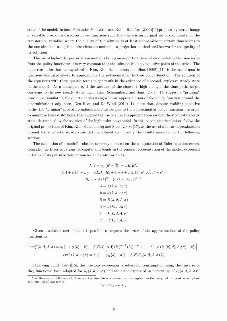
The evaluation of a model�s solution accuracy is based on the computation of Euler equation errors.
Consider the Euler equations for capital and bonds in the general representation of the model, expressed
in terms of its perturbation parameter and state variables:
��1� 3
�d0 � d
��= �EtR�
0
� [1 + � (k0 � k)] = �Et�0 [R0k + 1� � + � (k (k0; d0; A0;�)� k0)]
Rk = �A (k)��1
(h (k; d;A;�))1��
� = � (k; d;A;�)
h = h (k; d;A;�)
R = R (k; d;A;�)
� = � (k; d;A;�)
k0 = k (k; d;A;�)
d0 = d (k; d;A;�)
Given a solution method i, it is possible to express the error of the approximation of the policy
functions as:
errki (k; d;A;�) = �i [1 + � (k0i � k)]� �iEt�0i
h�A0i (k
0i)��1
(h0i)1��
+ 1� � + � (ki (k0i; d0i; A0i;�)� k0i)i
errdi (k; d;A;�) = �i�1� 3
�d0i � d
��� �iEtRi (k; d;A;�)�0i
Following Judd (1998)[15], the previous expression is solved for consumption using the (inverse of
the) functional form adopted for �i (k; d;A;�) and the error expressed in percentage of ci (k; d;A;�)5 .
5For the case of EDFI model, there is not a closed form solution for consumption, as the marginal utility of consumptionis a function of two terms:
�t = Uc;t + �t�c;t
9
It is common practice in the literature to express this error in absolute value and transformed by the
logarithm in base 10. As a consequence, a value of -3 means that, for every 1,000 dollars of consumption
measured in the model, one dollar is inaccurately measured; a value of -4 implies a one-dollar error for
every 10,000 dollars of consumption, and so on. The analysis of Euler error equations allows verifying
the solution�s accuracy outside the steady state of the model and checking error patterns with the exact
location of singularity points, where the quality of the approximated solution quickly deteriorates.
From the normalized Euler equation errors, two statistics are computed. First, trying to establish
an upper bound for the Euler error (see Aruoba, Fernández-Villaverde and Rubio-Ramírez, 2006 [5]),
the maximum value of the normalized Euler error is found among intervals of equally spaced 300 points
for each state variable (thus, the maximum value is picked among 3003 = 27; 000; 000 possible points
in the state space). The extreme values for intervals for each state variable are picked based on the
histogram of the simulated data. Second, in order to access the overall accuracy of the solution method,
the expected value of the errors is computed around relevant intervals describing the state variables of
the model. In order to compute the expected value, normalized Euler errors are integrated with respect
to the distribution of the most accurate solution based on the maximum value of the Euler error.
One test statistic often used to evaluate accuracy is the den Haan-Marcet (1994)[13] procedure. The
test is based on Euler equation errors of simulated data, noting that the de�nition of the error as a
function ut such that ut+1 = f (yt) � � (yt+1; yt+2; :::) ; where the true model is written as f (yt) =
Et [� (yt+1; yt+2; :::)] : Choosing any arbitrary function h (xt), the equality must hold:
Et [ut+1 h (xt)] = 0
The empirical counterpart of the equation above, generated from a solution method i; converges to
zero, as the size of the simulated series, T , goes to in�nity. Thus, under the null that the equation above
holds, the following test statistic converges to a �2 distribution with degrees of freedom equal to the size
of the instrument list h (xt) :
T�Bit�0 �
Ait��1 �
Bit��! �2nhx
Bit =1
T
TXt=1
uit+1 h�xit�
Ait =1
T
TXt=1
�uit+1
�2h�xit�h�xit�0
Since the whole procedure is based on simulated data, the recommended practice suggests to calculate
the test-statistic a large number of times and report the number of times the limit of the con�dence
interval is violated by the test. In this paper, the statistic is computed from 5000 simulations of time
series with 500 observations, around ten times larger than the usual sample size (annual frequency) in US
business cycle empirical analysis. It is well worth noting that den Haan-Marcet statistic tends to reject
the null hypothesis for large values of T : the larger the simulated sample, the higher is the probability
that the test-statistic captures the fact that policy functions drawing time series are approximations of
the true model. For the sake of robustness, the test is also run from 5000 simulations of a time series with
only 100 observations. The list of instruments includes a constant and lagged values of productivity and
capital. The inclusion of other lags or even the inclusion of debt simultaneously with capital generated
a near-singularity in the computation of matrix Ait. This means that the information provided by one
of the stock measures of the model (capital and foreign debt) is enough to describe the behavior of the
By assumption, the Euler error is calculated based on the consumption derived from the derivative of the utility function,Uc;t:
10
model up to that point.
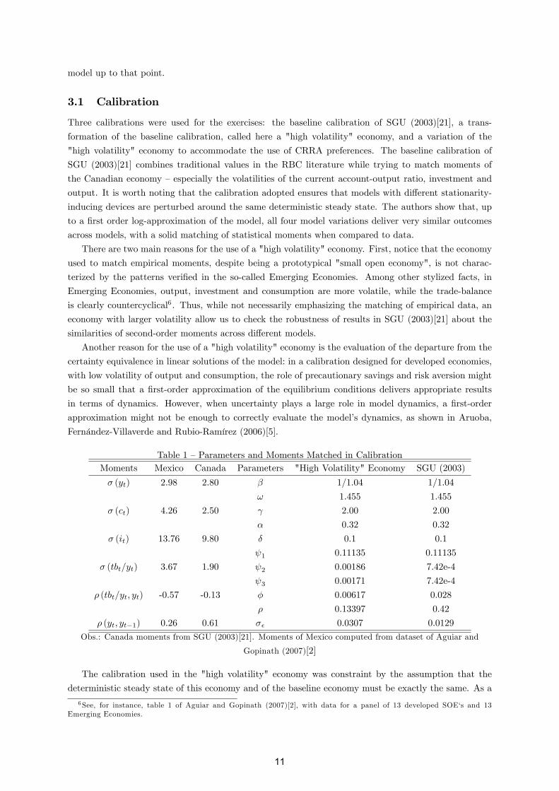
3.1 Calibration
Three calibrations were used for the exercises: the baseline calibration of SGU (2003)[21], a trans-
formation of the baseline calibration, called here a "high volatility" economy, and a variation of the
"high volatility" economy to accommodate the use of CRRA preferences. The baseline calibration of
SGU (2003)[21] combines traditional values in the RBC literature while trying to match moments of
the Canadian economy �especially the volatilities of the current account-output ratio, investment and
output. It is worth noting that the calibration adopted ensures that models with di¤erent stationarity-
inducing devices are perturbed around the same deterministic steady state. The authors show that, up
to a �rst order log-approximation of the model, all four model variations deliver very similar outcomes
across models, with a solid matching of statistical moments when compared to data.
There are two main reasons for the use of a "high volatility" economy. First, notice that the economy
used to match empirical moments, despite being a prototypical "small open economy", is not charac-
terized by the patterns veri�ed in the so-called Emerging Economies. Among other stylized facts, in
Emerging Economies, output, investment and consumption are more volatile, while the trade-balance
is clearly countercyclical6 . Thus, while not necessarily emphasizing the matching of empirical data, an
economy with larger volatility allow us to check the robustness of results in SGU (2003)[21] about the
similarities of second-order moments across di¤erent models.
Another reason for the use of a "high volatility" economy is the evaluation of the departure from the
certainty equivalence in linear solutions of the model: in a calibration designed for developed economies,
with low volatility of output and consumption, the role of precautionary savings and risk aversion might
be so small that a �rst-order approximation of the equilibrium conditions delivers appropriate results
in terms of dynamics. However, when uncertainty plays a large role in model dynamics, a �rst-order
approximation might not be enough to correctly evaluate the model�s dynamics, as shown in Aruoba,
Fernández-Villaverde and Rubio-Ramírez (2006)[5].
Table 1 �Parameters and Moments Matched in CalibrationMoments Mexico Canada Parameters "High Volatility" Economy SGU (2003)
� (yt) 2.98 2.80 � 1/1.04 1/1.04
! 1.455 1.455
� (ct) 4.26 2.50 2.00 2.00
� 0.32 0.32
� (it) 13.76 9.80 � 0.1 0.1
1 0.11135 0.11135
� (tbt=yt) 3.67 1.90 2 0.00186 7.42e-4
3 0.00171 7.42e-4
� (tbt=yt; yt) -0.57 -0.13 � 0.00617 0.028
� 0.13397 0.42
� (yt; yt�1) 0.26 0.61 �� 0.0307 0.0129
Obs.: Canada moments from SGU (2003)[21]. Moments of Mexico computed from dataset of Aguiar and
Gopinath (2007)[2]
The calibration used in the "high volatility" economy was constraint by the assumption that the
deterministic steady state of this economy and of the baseline economy must be exactly the same. As a
6See, for instance, table 1 of Aguiar and Gopinath (2007)[2], with data for a panel of 13 developed SOE�s and 13Emerging Economies.
11
consequence, only three parameters that have no e¤ect in the computation of the deterministic steady
state were altered from the baseline calibration: the persistence and volatility of productivity, � and
�; and the adjustment cost of capital, �; were used to match the autocorrelation of output and the
volatility of consumption and investment characterizing the Mexican economy. The strategy followed
SGU (2003)[21], in the sense that the moments were computed using the EDFI model solved by log-
linearizing the equilibrium conditions. Parameters 2 and 3, characterizing DEIR and PAC models,
matched the simulated volatility of the trade balance-output ratio generated in the EDFI model.
There are three main reasons for using the Mexican economy as the prototypical "high volatility"
economy. First, the second moments of that economy, shown in table 1, highlight some of the main
di¤erences between developed SOE�s and Emerging Economies, namely: a) consumption is more volatile
than output in Mexico, while the opposite is true in Canada; b) investment is more volatile in Mexico
than in Canada; c) trade balance-output ratio is slightly countercyclical in Canada, while this correlation
in Mexico is much more pronounced. The second reason for using data from Mexico is availability: the
dataset compiled by Aguiar and Gopinath (2007)[2], available at the authors�websites, allows compar-
isons between this economy and a set of Emerging and Developed Economies. Finally, the Mexican
dataset was used, at a quarterly frequency, by Seoane (2011)[22] to calibrate the set of parameters for all
economies described here �thus, there is base for comparison with some of the results presented here7 .
The calibration strategy adopted here di¤ers from Seoane (2011)[22], as the author is more interested
in the �tting of the basic formulations of the RBC model for Emerging Economies. Seoane (2011)[22]
estimated the common parameters across models using Simulated Method of Moments (SMM) on the
second-order approximation of EDFI model, with the parameters describing DEIR and PAC models
calibrated to match the volatility of the current account-GDP ratio in the second-order approximation
of the model. In terms of results, the calibration of the same model using quarterly data for the Mexican
economy shows that statistical moments signi�cantly di¤er across models. In particular, DEIR model
has problems in adjusting to the countercyclical trade balance.
Finally, the economy with CRRA preferences follows the same calibration strategy described above,
trying to match the dynamics of the "high volatility" economy. The CRRA economy requires di¤erent
assumptions with respect to the steady state of labor supply and the trade balance-output ratio, resulting
in a di¤erent set of values even for the common parameters of the economy with GHH preferences. Details
of the CRRA economy, including the calibration, are presented in section 6.
4 Properties of Baseline Economy
This section explores the solution accuracy of EDFE, EDFI, DEIR and PAC models and extends the
evaluation of models�global and local dynamics in extreme points of the state variables. The analysis
follow three steps: �rst, the accuracy of each solution is evaluated using the methods presented in
Aruoba, Fernández-Villaverde and Rubio-Ramírez (2006)[5] up to a third-order approximation of the
equilibrium conditions; second, the computation of relevant second moments of the model replicates
the exercise presented in Seoane (2011)[22]; �nally, the moments and impulse response functions are
computed assuming initial states of low capital in each economy.
The statistical moments are computed based on simulations of the model. Each model is simulated
for 50,000 periods, with the �rst 1,000 observations dropped and the remaining used to compute the
moments8 . Statistical moments were computed using �rst, second and third-order approximations of
7 In order to generate moments comparable to SGU (2003) [21], data from Mexico in Aguiar and Gopinath (2007)[2] wasreduced to annual frequency and the logarithm of data was detrended using a quadratic polynomial. This is the procedureapplied in Mendoza (1991)[20] for data from Canada, where SGU (2003) [21] picked parameters and empirical moments tocompare the outcome of the model.
8 In order to make comparisons relevant, all simulations of ergodic moments started at the deterministic steady state of
12
the equilibrium conditions with variables in levels. In order to generate results comparable with SGU
(2003)[21] and Seoane (2011)[22], simulated values were transformed to logarithms9 . All simulations
based on non-linear approximations of the policy functions incorporated the "pruning" procedure de-
scribed in Kim, Kim, Schaumburg and Sims (2008) [17], as described in section 3.
Table 2 �Den Haan-Marcet Statistic �Baseline CalibrationOrder 1 2 3
< 5% > 95% < 5% > 95% < 5% > 95%
EDFE
Bonds 5.26 4.74 5.02 4.84 5.00 4.86
Capital 5.28 5.06 5.06 4.76 5.12 4.78
EDFI
Bonds 5.10 4.66 5.10 4.84 5.08 4.84
Capital 5.30 4.60 5.02 4.84 5.00 4.82
DEIR
Bonds 5.16 6.30 5.10 5.50 5.12 5.46
Capital 5.14 7.04 4.90 6.02 4.86 6.74
PAC
Bonds 5.20 6.08 5.18 5.72 5.16 5.68
Capital 5.12 7.10 5.02 5.08 5.00 5.78
Obs.: results show percentage of simulations below (above) the 5% (95%)
critical value of the chi-square distribution with 3 degrees of freedom.
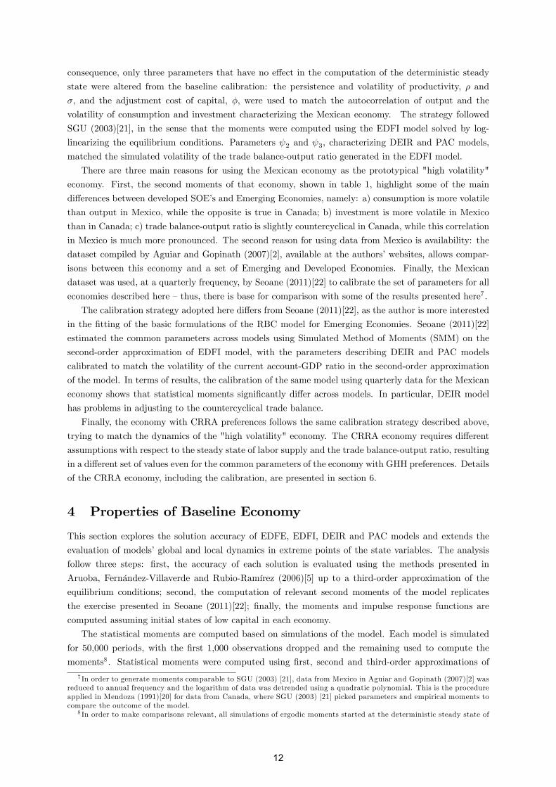
Starting with the characterization of solution�s accuracy, table 2 presents the den Haan-Marcet test,
showing that perturbation methods do indeed a good job characterizing the dynamics of the baseline
economy. Irrespective of the model or the Euler equation evaluated, the distribution of the test statistic
is most of the time located inside the 90% con�dence interval. The distribution of the test is slightly
skewed to the left in models based on the endogenous discount factor, while the distribution is slightly
skewed to the right in models based on the level of foreign debt.
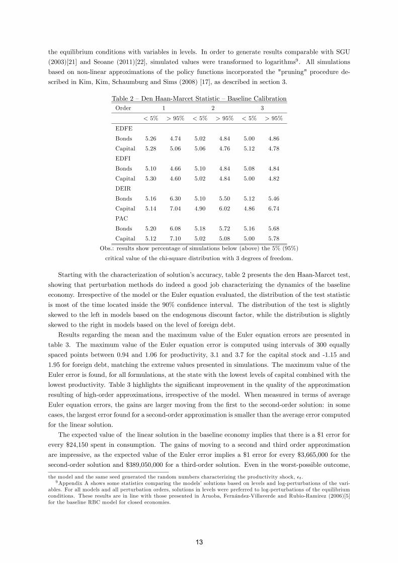
Results regarding the mean and the maximum value of the Euler equation errors are presented in
table 3. The maximum value of the Euler equation error is computed using intervals of 300 equally
spaced points between 0.94 and 1.06 for productivity, 3.1 and 3.7 for the capital stock and -1.15 and
1.95 for foreign debt, matching the extreme values presented in simulations. The maximum value of the
Euler error is found, for all formulations, at the state with the lowest levels of capital combined with the
lowest productivity. Table 3 highlights the signi�cant improvement in the quality of the approximation
resulting of high-order approximations, irrespective of the model. When measured in terms of average
Euler equation errors, the gains are larger moving from the �rst to the second-order solution: in some
cases, the largest error found for a second-order approximation is smaller than the average error computed
for the linear solution.
The expected value of the linear solution in the baseline economy implies that there is a $1 error for
every $24,150 spent in consumption. The gains of moving to a second and third order approximation
are impressive, as the expected value of the Euler error implies a $1 error for every $3,665,000 for the
second-order solution and $389,050,000 for a third-order solution. Even in the worst-possible outcome,
the model and the same seed generated the random numbers characterizing the productivity shock, �t.9Appendix A shows some statistics comparing the models�solutions based on levels and log-perturbations of the vari-
ables. For all models and all perturbation orders, solutions in levels were preferred to log-perturbations of the equilibriumconditions. These results are in line with those presented in Aruoba, Fernández-Villaverde and Rubio-Ramirez (2006)[5]for the baseline RBC model for closed economies.
13
the maximum error for a third-order approximation implies a $1 for every $181,950, more than 7 times
smaller than the expected error of the linear solution.
Table 3 �Euler Equation Errors �Baseline Calibration
Order 1 2 3
Max(EE) E(EE) Max(EE) E(EE) Max(EE) E(EE)
EDFE
Bonds -3.099 -4.380 -4.750 -6.619 -5.991 -9.058
Capital -3.108 -4.407 -4.758 -6.654 -5.993 -9.280
EDFI
Bonds -3.162 -4.324 -3.804 -6.567 -4.334 -8.576
Capital -3.175 -4.361 -3.809 -6.659 -4.338 -8.978
DEIR
Bonds -3.184 -4.341 -4.282 -6.363 -5.080 -7.806
Capital -3.146 -4.421 -4.174 -6.322 -4.326 -7.540
PAC
Bonds -3.138 -4.408 -4.771 -6.659 -6.000 -8.524
Capital -3.144 -4.421 -4.783 -6.667 -6.001 -8.954
Obs.: results measured as logarithms of base 10: a value of -4 shows an error of $1 for every $10,000
spent in consumption; a value of -5 represents an error of $1 for every $100,000; and so on.
Figure 1: Euler Errors - Baseline Calibration
Figure 1 show the conditional mean of the Euler errors computed at two di¤erent dimensions of
the state space: graphs in the �rst line of �gure 1 assume that foreign debt and productivity are at
14
the deterministic steady state value, with the horizontal axe showing the same range of capital in the
histograms of �gure 2; the second line of graphs follows the same procedure, with capital at the deter-
ministic steady state and the horizontal axe showing the relevant values of foreign debt. The shaded
area is the histogram of the third-order approximation, plotted here in order to capture the accuracy of
the solution method in the relevant region of the state space. From the picture, it is clear that linear
approximations of the equilibrium conditions are dominated by high-order solutions, even when moving
far outside the deterministic steady state. Non-linear approximations errors are between two and four
orders of magnitude smaller than the linear perturbation of the model, depending on the region of the
state space being compared.
The picture also shows that the largest gains seems to come from a better characterization of the
policy functions describing foreign debt: according to table 3, the worst �t of a third-order solution is
found at the DEIR model, based on average Euler errors; in that model, the similarity between the plots
of the second and third-order solutions�errors across the relevant space of foreign debt suggest it is the
description of this variable that conditions the quality of the approximation.
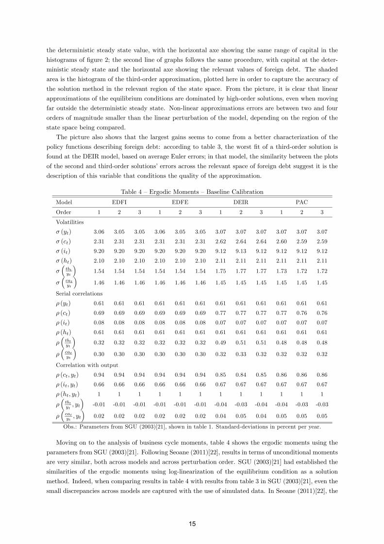
Table 4 �Ergodic Moments �Baseline Calibration
Model EDFI EDFE DEIR PAC
Order 1 2 3 1 2 3 1 2 3 1 2 3
Volatilities
� (yt) 3.06 3.05 3.05 3.06 3.05 3.05 3.07 3.07 3.07 3.07 3.07 3.07
� (ct) 2.31 2.31 2.31 2.31 2.31 2.31 2.62 2.64 2.64 2.60 2.59 2.59
� (it) 9.20 9.20 9.20 9.20 9.20 9.20 9.12 9.13 9.12 9.12 9.12 9.12
� (ht) 2.10 2.10 2.10 2.10 2.10 2.10 2.11 2.11 2.11 2.11 2.11 2.11
��tbtyt
�1.54 1.54 1.54 1.54 1.54 1.54 1.75 1.77 1.77 1.73 1.72 1.72
��catyt
�1.46 1.46 1.46 1.46 1.46 1.46 1.45 1.45 1.45 1.45 1.45 1.45
Serial correlations
� (yt) 0.61 0.61 0.61 0.61 0.61 0.61 0.61 0.61 0.61 0.61 0.61 0.61
� (ct) 0.69 0.69 0.69 0.69 0.69 0.69 0.77 0.77 0.77 0.77 0.76 0.76
� (it) 0.08 0.08 0.08 0.08 0.08 0.08 0.07 0.07 0.07 0.07 0.07 0.07
� (ht) 0.61 0.61 0.61 0.61 0.61 0.61 0.61 0.61 0.61 0.61 0.61 0.61
��tbtyt
�0.32 0.32 0.32 0.32 0.32 0.32 0.49 0.51 0.51 0.48 0.48 0.48
��catyt
�0.30 0.30 0.30 0.30 0.30 0.30 0.32 0.33 0.32 0.32 0.32 0.32
Correlation with output
� (ct; yt) 0.94 0.94 0.94 0.94 0.94 0.94 0.85 0.84 0.85 0.86 0.86 0.86
� (it; yt) 0.66 0.66 0.66 0.66 0.66 0.66 0.67 0.67 0.67 0.67 0.67 0.67
� (ht; yt) 1 1 1 1 1 1 1 1 1 1 1 1
��tbtyt; yt
�-0.01 -0.01 -0.01 -0.01 -0.01 -0.01 -0.04 -0.03 -0.04 -0.04 -0.03 -0.03
��catyt; yt
�0.02 0.02 0.02 0.02 0.02 0.02 0.04 0.05 0.04 0.05 0.05 0.05
Obs.: Parameters from SGU (2003)[21], shown in table 1. Standard-deviations in percent per year.
Moving on to the analysis of business cycle moments, table 4 shows the ergodic moments using the
parameters from SGU (2003)[21]. Following Seoane (2011)[22], results in terms of unconditional moments
are very similar, both across models and across perturbation order. SGU (2003)[21] had established the
similarities of the ergodic moments using log-linearization of the equilibrium condition as a solution
method. Indeed, when comparing results in table 4 with results from table 3 in SGU (2003)[21], even the
small discrepancies across models are captured with the use of simulated data. In Seoane (2011)[22], the
15
result in SGU (2003)[21] is expanded to second and third-order approximations of the models. As the
solution based on the third-order approximation is a re�nement of the stable path found in the second-
order approximation, it could be argued that the ergodic distribution of the model could be a¤ected by
the solution method. However, given the calibration matching Canadian moments, the use of non-linear
solutions does not alter the main results.
The similarities of the ergodic moments are also re�ected in the empirical distribution of the state
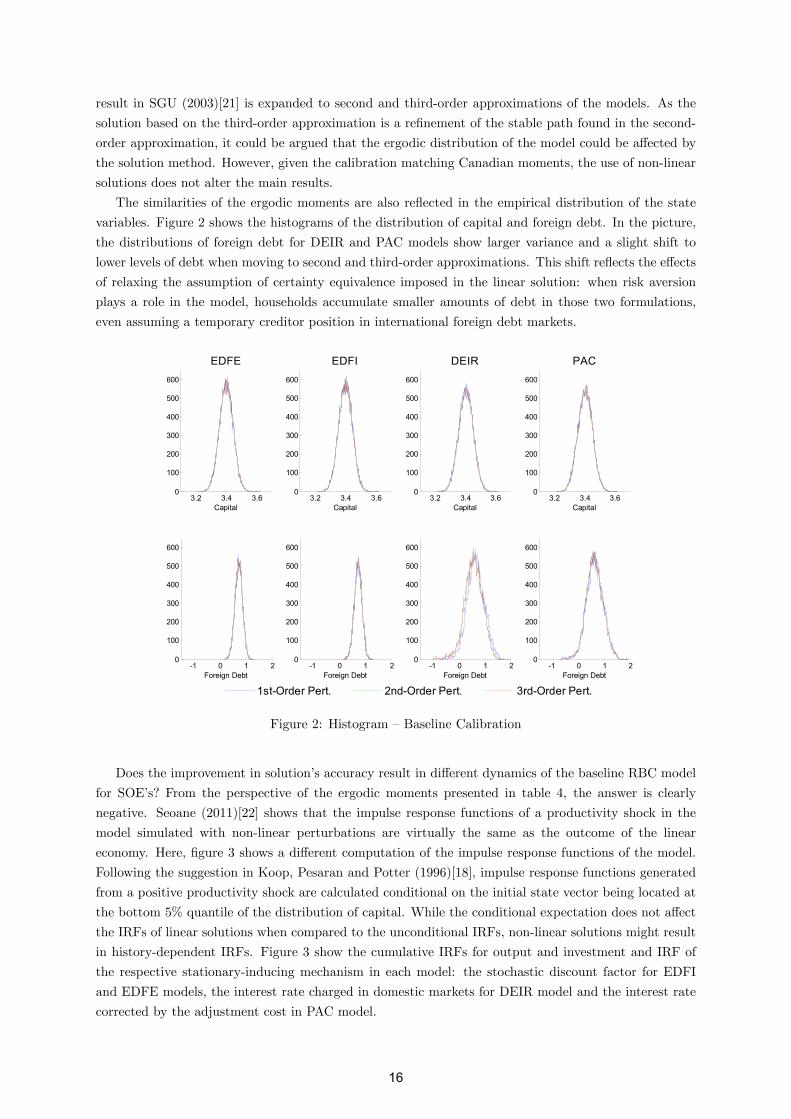
variables. Figure 2 shows the histograms of the distribution of capital and foreign debt. In the picture,
the distributions of foreign debt for DEIR and PAC models show larger variance and a slight shift to
lower levels of debt when moving to second and third-order approximations. This shift re�ects the e¤ects
of relaxing the assumption of certainty equivalence imposed in the linear solution: when risk aversion
plays a role in the model, households accumulate smaller amounts of debt in those two formulations,
even assuming a temporary creditor position in international foreign debt markets.
3.2 3.4 3.60
100
200
300
400
500
600
Capital
EDFE
-1 0 1 20
100
200
300
400
500
600
Foreign Debt
3.2 3.4 3.60
100
200
300
400
500
600
Capital
EDFI
-1 0 1 20
100
200
300
400
500
600
Foreign Debt
3.2 3.4 3.60
100
200
300
400
500
600
Capital
DEIR
-1 0 1 20
100
200
300
400
500
600
Foreign Debt
3.2 3.4 3.60
100
200
300
400
500
600
Capital
PAC
-1 0 1 20
100
200
300
400
500
600
Foreign Debt
1st-Order Pert. 2nd-Order Pert. 3rd-Order Pert.
Figure 2: Histogram �Baseline Calibration
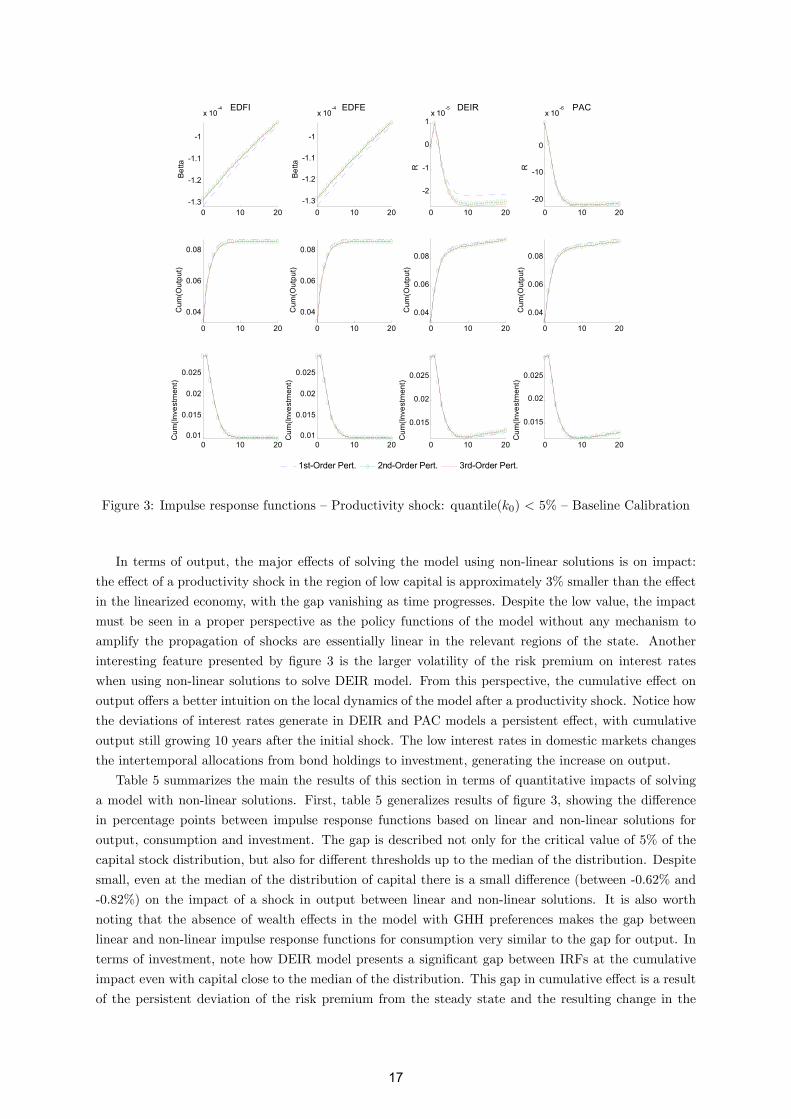
Does the improvement in solution�s accuracy result in di¤erent dynamics of the baseline RBC model
for SOE�s? From the perspective of the ergodic moments presented in table 4, the answer is clearly
negative. Seoane (2011)[22] shows that the impulse response functions of a productivity shock in the
model simulated with non-linear perturbations are virtually the same as the outcome of the linear
economy. Here, �gure 3 shows a di¤erent computation of the impulse response functions of the model.
Following the suggestion in Koop, Pesaran and Potter (1996)[18], impulse response functions generated
from a positive productivity shock are calculated conditional on the initial state vector being located at
the bottom 5% quantile of the distribution of capital. While the conditional expectation does not a¤ect
the IRFs of linear solutions when compared to the unconditional IRFs, non-linear solutions might result
in history-dependent IRFs. Figure 3 show the cumulative IRFs for output and investment and IRF of
the respective stationary-inducing mechanism in each model: the stochastic discount factor for EDFI
and EDFE models, the interest rate charged in domestic markets for DEIR model and the interest rate
corrected by the adjustment cost in PAC model.
16
0 10 20-1.3
-1.2
-1.1
-1
x 10-4 EDFI
Bet
ta
0 10 20
0.04
0.06
0.08
Cum
(Out
put)
0 10 200.01
0.015
0.02
0.025
Cum
(Inve
stm
ent)
0 10 20-1.3
-1.2
-1.1
-1
x 10-4 EDFE
Bet
ta
0 10 20
0.04
0.06
0.08
Cum
(Out
put)
0 10 200.01
0.015
0.02
0.025
Cum
(Inve
stm
ent)
0 10 20
-2
-1
0
1x 10
-5 DEIR
R
0 10 20
0.04
0.06
0.08
Cum
(Out
put)
0 10 20
0.015
0.02
0.025
Cum
(Inve
stm
ent)
0 10 20
-20
-10
0
x 10-6 PAC
R
0 10 20
0.04
0.06
0.08
Cum
(Out
put)
0 10 20
0.015
0.02
0.025
Cum
(Inve
stm
ent)
1st-Order Pert. 2nd-Order Pert. 3rd-Order Pert.
Figure 3: Impulse response functions �Productivity shock: quantile(k0) < 5% �Baseline Calibration
In terms of output, the major e¤ects of solving the model using non-linear solutions is on impact:
the e¤ect of a productivity shock in the region of low capital is approximately 3% smaller than the e¤ect
in the linearized economy, with the gap vanishing as time progresses. Despite the low value, the impact
must be seen in a proper perspective as the policy functions of the model without any mechanism to
amplify the propagation of shocks are essentially linear in the relevant regions of the state. Another
interesting feature presented by �gure 3 is the larger volatility of the risk premium on interest rates
when using non-linear solutions to solve DEIR model. From this perspective, the cumulative e¤ect on
output o¤ers a better intuition on the local dynamics of the model after a productivity shock. Notice how
the deviations of interest rates generate in DEIR and PAC models a persistent e¤ect, with cumulative
output still growing 10 years after the initial shock. The low interest rates in domestic markets changes
the intertemporal allocations from bond holdings to investment, generating the increase on output.
Table 5 summarizes the main the results of this section in terms of quantitative impacts of solving
a model with non-linear solutions. First, table 5 generalizes results of �gure 3, showing the di¤erence
in percentage points between impulse response functions based on linear and non-linear solutions for
output, consumption and investment. The gap is described not only for the critical value of 5% of the
capital stock distribution, but also for di¤erent thresholds up to the median of the distribution. Despite
small, even at the median of the distribution of capital there is a small di¤erence (between -0.62% and
-0.82%) on the impact of a shock in output between linear and non-linear solutions. It is also worth
noting that the absence of wealth e¤ects in the model with GHH preferences makes the gap between
linear and non-linear impulse response functions for consumption very similar to the gap for output. In
terms of investment, note how DEIR model presents a signi�cant gap between IRFs at the cumulative
impact even with capital close to the median of the distribution. This gap in cumulative e¤ect is a result
of the persistent deviation of the risk premium from the steady state and the resulting change in the
17
relative price between capital rent and bond returns. The gap is also larger in the PAC model, when
compared to EDFE and EDFI models, but the e¤ect on relative prices is magni�ed in DEIR model due
to the functional form adopted to describe the behavior of risk premium.
Table 5 �Conditional Moments �Baseline CalibrationEDFI EDFE DEIR PAC
Gap between IRFs: Output, 3rd to 1st�order: impact (cumulative)Quantile(K0) < 0.05 -2.80% (-1.82%) -2.98% (-1.93%) -2.84% (-1.47%) -2.84% (-1.95%)
Quantile(K0) < 0.10 -2.42% (-1.58%) -2.42% (-1.58%) -2.35% (-1.18%) -2.34% (-1.57%)
Quantile(K0) < 0.25 -1.61% (-1.03%) -1.61% (-1.03%) -1.49% (-0.69%) -1.50% (-0.93%)
Quantile(K0) < 0.50 -0.82% (-0.50%) -0.82% (-0.50%) -0.62% (-0.22%) -0.63% (-0.38%)
Gap between IRFs: Consumption, 3rd to 1st�order: impact (cumulative)Quantile(K0) < 0.05 -2.80% (-2.04%) -2.99% (-2.18%) -2.67% (-1.24%) -2.81% (-2.04%)
Quantile(K0) < 0.10 -2.42% (-1.77%) -2.43% (-1.79%) -2.20% (-0.99%) -2.31% (-1.64%)
Quantile(K0) < 0.25 -1.61% (-1.16%) -1.62% (-1.17%) -1.39% (-0.54%) -1.48% (-0.98%)
Quantile(K0) < 0.50 -0.82% (-0.57%) -0.82% (-0.57%) -0.56% (-0.13%) -0.62% (-0.39%)
Gap between IRFs: Investment, 3rd to 1st�order: impact (cumulative)Quantile(K0) < 0.05 -0.49% (-0.63%) -0.53% (-0.67%) -0.60% (2.67%) -0.56% (-1.17%)
Quantile(K0) < 0.10 -0.42% (-0.54%) -0.42% (-0.53%) -0.50% (2.27%) -0.46% (-0.94%)
Quantile(K0) < 0.25 -0.28% (-0.34%) -0.28% (-0.33%) -0.31% (1.73%) -0.29% (-0.56%)
Quantile(K0) < 0.50 -0.15% (-0.15%) -0.14% (-0.14%) -0.14% (1.11%) -0.12% (-0.22%)
Debt-to-GDP ratio: median �standard-deviation (SS = 0.50)
1st�order 0.490; 0.10 0.491; 0.10 0.434; 0.23 0.438; 0.22
2nd�order 0.484; 0.10 0.484; 0.10 0.383; 0.24 0.418; 0.22
3rd�order 0.484; 0.10 0.484; 0.10 0.384; 0.24 0.418; 0.22
Second, the �nal block of results presented in table 5 shows that the e¤ects of precautionary savings
and risk aversion, present in non-linear solutions, result in a reduction of the median debt-to-GDP ratio
up to 5 percentage points, when compared to results based on the linear approximation of equilibrium.
For all models, the median of the distribution of the debt-to-GDP ratio is below the steady state of
the economy, but this gap for DEIR and PAC models is not only signi�cant, but increases with the
use of non-linear solutions. On the debt-to-GDP ratio, it is also worth mentioning that a second-order
approximation seems to be enough to adjust the level of this variable for the nonlinearity of the model, as
results on the median and standard-deviation of this ratio are very similar between second and third-order
approximations.
5 The "High Volatility" Economy
As shown in section 3.1, the "high volatility" economy is characterized by a signi�cant increase in
volatility of the productivity shock, small adjustment cost of investment and low persistence of output.
The main idea of the "high volatility" economy is to evaluate the quality of the solution once the overall
volatility of the economy is increased to reasonable values found in the literature, at the expense of the
match of additional moments of data. From this perspective, the "high volatility" economy replicates
second moments of Emerging Economies in a baseline model suited for developed economies. As an
example, the "high volatility" calibration shows a positive correlation between trade balance and current
account with output, when the correlation for the baseline economy, �tting data for Canada, was close to
zero and negative in data for Mexico. The adjustment of the model in order to �t the correlation would
18
come at the cost of changing other structural parameters and, as a consequence, the deterministic steady
state of the model. The analysis of �tting of the basic RBC model is presented in Seoane (2011)[22],
where the author estimates the model to match a complete set of moments of the Mexican economy.
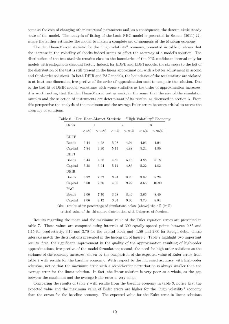
The den Haan-Marcet statistic for the "high volatility" economy, presented in table 6, shows that
the increase in the volatility of shocks indeed seems to a¤ect the accuracy of a model�s solution. The
distribution of the test statistic remains close to the boundaries of the 90% con�dence interval only for
models with endogenous discount factor. Indeed, for EDFE and EDFI models, the skewness to the left of
the distribution of the test is still present in the linear approximation, with a better adjustment in second
and third-order solutions. In both DEIR and PAC models, the boundaries of the test statistic are violated
in at least one dimension, irrespective of the order of approximation used to compute the solution. Due
to the bad �t of DEIR model, sometimes with worse statistics as the order of approximation increases,
it is worth noting that the den Haan-Marcet test is weak, in the sense that the size of the simulation
samples and the selection of instruments are determinant of its results, as discussed in section 3. From
this perspective the analysis of the maximum and the average Euler errors becomes critical to access the
accuracy of solutions.
Table 6 �Den Haan-Marcet Statistic �"High Volatility" Economy
Order 1 2 3
< 5% > 95% < 5% > 95% < 5% > 95%
EDFE
Bonds 5.44 4.58 5.08 4.94 4.96 4.94
Capital 5.84 3.30 5.14 4.88 5.24 4.80
EDFI
Bonds 5.44 4.58 4.80 5.16 4.88 5.18
Capital 5.28 3.94 5.14 4.86 5.22 4.82
DEIR
Bonds 3.92 7.52 3.84 8.20 3.82 8.28
Capital 6.60 2.60 4.00 9.22 3.66 10.90
PAC
Bonds 4.00 7.70 3.68 8.46 3.66 8.40
Capital 7.06 2.12 3.84 9.06 3.78 8.84
Obs.: results show percentage of simulations below (above) the 5% (95%)
critical value of the chi-square distribution with 3 degrees of freedom.
Results regarding the mean and the maximum value of the Euler equation errors are presented in
table 7. Those values are computed using intervals of 300 equally spaced points between 0.85 and
1.15 for productivity, 3.10 and 3.70 for the capital stock and -1.50 and 2.00 for foreign debt. These
intervals match the distributions presented in the histogram of �gure 5. Table 7 highlight two important
results: �rst, the signi�cant improvement in the quality of the approximation resulting of high-order
approximations, irrespective of the model formulation; second, the need for high-order solutions as the
variance of the economy increases, shown by the comparison of the expected value of Euler errors from
table 7 with results for the baseline economy. With respect to the increased accuracy with high-order
solutions, notice that the maximum error with a second-order perturbation is always smaller than the
average error for the linear solution. In fact, the linear solution is very poor as a whole, as the gap
between the maximum and the average Euler error is very small.
Comparing the results of table 7 with results from the baseline economy in table 3, notice that the
expected value and the maximum value of Euler errors are higher for the "high volatility" economy
than the errors for the baseline economy. The expected value for the Euler error in linear solutions
19
for the "high volatility" economy implies a solution error of approximately $1 for every $3,150 spent in
consumption, an error much higher than the one found with the baseline calibration. It is worth noting,
however, that, depending on the model, the maximum Euler error found in table 3 is similar to the
value presented in table 7, meaning that in some dimensions of the states (normally, the extremes of
the distribution), the quality of the approximation is very similar, irrespective of the volatility of the
economy.
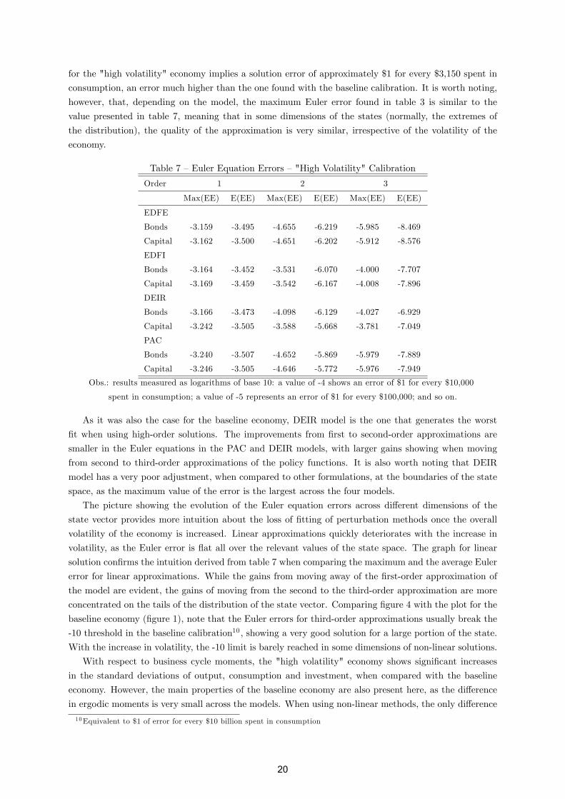
Table 7 �Euler Equation Errors �"High Volatility" Calibration
Order 1 2 3
Max(EE) E(EE) Max(EE) E(EE) Max(EE) E(EE)
EDFE
Bonds -3.159 -3.495 -4.655 -6.219 -5.985 -8.469
Capital -3.162 -3.500 -4.651 -6.202 -5.912 -8.576
EDFI
Bonds -3.164 -3.452 -3.531 -6.070 -4.000 -7.707
Capital -3.169 -3.459 -3.542 -6.167 -4.008 -7.896
DEIR
Bonds -3.166 -3.473 -4.098 -6.129 -4.027 -6.929
Capital -3.242 -3.505 -3.588 -5.668 -3.781 -7.049
PAC
Bonds -3.240 -3.507 -4.652 -5.869 -5.979 -7.889
Capital -3.246 -3.505 -4.646 -5.772 -5.976 -7.949
Obs.: results measured as logarithms of base 10: a value of -4 shows an error of $1 for every $10,000
spent in consumption; a value of -5 represents an error of $1 for every $100,000; and so on.
As it was also the case for the baseline economy, DEIR model is the one that generates the worst
�t when using high-order solutions. The improvements from �rst to second-order approximations are
smaller in the Euler equations in the PAC and DEIR models, with larger gains showing when moving
from second to third-order approximations of the policy functions. It is also worth noting that DEIR
model has a very poor adjustment, when compared to other formulations, at the boundaries of the state
space, as the maximum value of the error is the largest across the four models.
The picture showing the evolution of the Euler equation errors across di¤erent dimensions of the
state vector provides more intuition about the loss of �tting of perturbation methods once the overall
volatility of the economy is increased. Linear approximations quickly deteriorates with the increase in
volatility, as the Euler error is �at all over the relevant values of the state space. The graph for linear
solution con�rms the intuition derived from table 7 when comparing the maximum and the average Euler
error for linear approximations. While the gains from moving away of the �rst-order approximation of
the model are evident, the gains of moving from the second to the third-order approximation are more
concentrated on the tails of the distribution of the state vector. Comparing �gure 4 with the plot for the
baseline economy (�gure 1), note that the Euler errors for third-order approximations usually break the
-10 threshold in the baseline calibration10 , showing a very good solution for a large portion of the state.
With the increase in volatility, the -10 limit is barely reached in some dimensions of non-linear solutions.
With respect to business cycle moments, the "high volatility" economy shows signi�cant increases
in the standard deviations of output, consumption and investment, when compared with the baseline
economy. However, the main properties of the baseline economy are also present here, as the di¤erence
in ergodic moments is very small across the models. When using non-linear methods, the only di¤erence
10Equivalent to $1 of error for every $10 billion spent in consumption
20
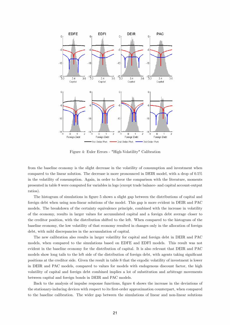
Figure 4: Euler Errors - "High-Volatility" Calibration
from the baseline economy is the slight decrease in the volatility of consumption and investment when
compared to the linear solution. The decrease is more pronounced in DEIR model, with a drop of 0.5%
in the volatility of consumption. Again, in order to favor the comparison with the literature, moments
presented in table 8 were computed for variables in logs (except trade balance- and capital account-output
ratios).
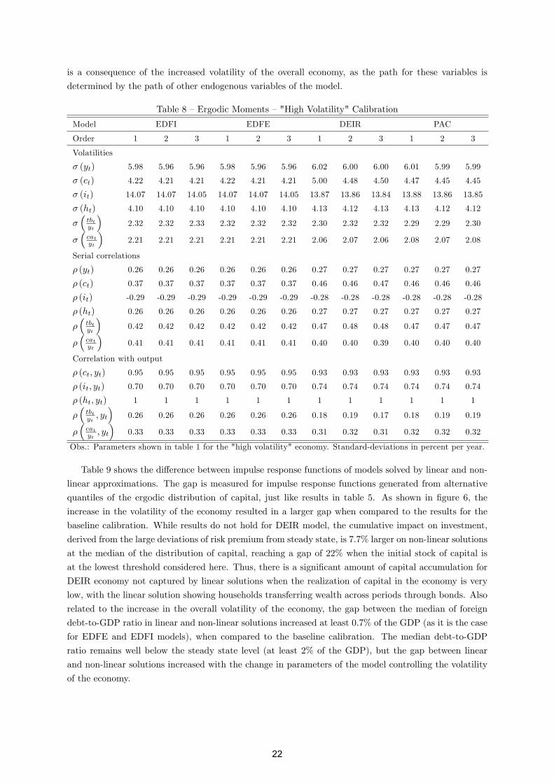
The histogram of simulations in �gure 5 shows a slight gap between the distributions of capital and
foreign debt when using non-linear solutions of the model. This gap is more evident in DEIR and PAC
models. The breakdown of the certainty equivalence principle, combined with the increase in volatility
of the economy, results in larger values for accumulated capital and a foreign debt average closer to
the creditor position, with the distribution shifted to the left. When compared to the histogram of the
baseline economy, the low volatility of that economy resulted in changes only in the allocation of foreign
debt, with mild discrepancies in the accumulation of capital.
The new calibration also results in larger volatility for capital and foreign debt in DEIR and PAC
models, when compared to the simulations based on EDFE and EDFI models. This result was not
evident in the baseline economy for the distribution of capital. It is also relevant that DEIR and PAC
models show long tails to the left side of the distribution of foreign debt, with agents taking signi�cant
positions at the creditor side. Given the result in table 8 that the ergodic volatility of investment is lower
in DEIR and PAC models, compared to values for models with endogenous discount factor, the high
volatility of capital and foreign debt combined implies a lot of substitution and arbitrage movements
between capital and foreign bonds in DEIR and PAC models.
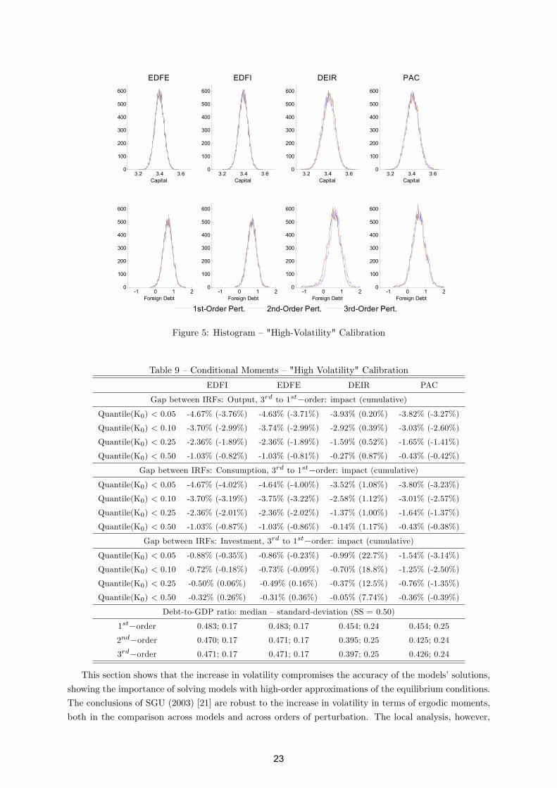
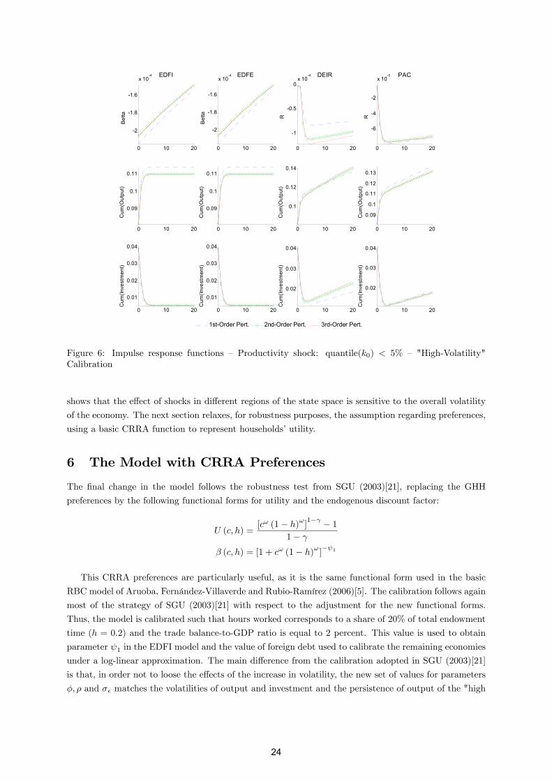
Back to the analysis of impulse response functions, �gure 6 shows the increase in the deviations of
the stationary-inducing devices with respect to its �rst-order approximation counterpart, when compared
to the baseline calibration. The wider gap between the simulations of linear and non-linear solutions
21
is a consequence of the increased volatility of the overall economy, as the path for these variables is
determined by the path of other endogenous variables of the model.
Table 8 �Ergodic Moments �"High Volatility" Calibration
Model EDFI EDFE DEIR PAC
Order 1 2 3 1 2 3 1 2 3 1 2 3
Volatilities
� (yt) 5.98 5.96 5.96 5.98 5.96 5.96 6.02 6.00 6.00 6.01 5.99 5.99
� (ct) 4.22 4.21 4.21 4.22 4.21 4.21 5.00 4.48 4.50 4.47 4.45 4.45
� (it) 14.07 14.07 14.05 14.07 14.07 14.05 13.87 13.86 13.84 13.88 13.86 13.85
� (ht) 4.10 4.10 4.10 4.10 4.10 4.10 4.13 4.12 4.13 4.13 4.12 4.12
��tbtyt
�2.32 2.32 2.33 2.32 2.32 2.32 2.30 2.32 2.32 2.29 2.29 2.30
��catyt
�2.21 2.21 2.21 2.21 2.21 2.21 2.06 2.07 2.06 2.08 2.07 2.08
Serial correlations
� (yt) 0.26 0.26 0.26 0.26 0.26 0.26 0.27 0.27 0.27 0.27 0.27 0.27
� (ct) 0.37 0.37 0.37 0.37 0.37 0.37 0.46 0.46 0.47 0.46 0.46 0.46
� (it) -0.29 -0.29 -0.29 -0.29 -0.29 -0.29 -0.28 -0.28 -0.28 -0.28 -0.28 -0.28
� (ht) 0.26 0.26 0.26 0.26 0.26 0.26 0.27 0.27 0.27 0.27 0.27 0.27
��tbtyt
�0.42 0.42 0.42 0.42 0.42 0.42 0.47 0.48 0.48 0.47 0.47 0.47
��catyt
�0.41 0.41 0.41 0.41 0.41 0.41 0.40 0.40 0.39 0.40 0.40 0.40
Correlation with output
� (ct; yt) 0.95 0.95 0.95 0.95 0.95 0.95 0.93 0.93 0.93 0.93 0.93 0.93
� (it; yt) 0.70 0.70 0.70 0.70 0.70 0.70 0.74 0.74 0.74 0.74 0.74 0.74
� (ht; yt) 1 1 1 1 1 1 1 1 1 1 1 1
��tbtyt; yt
�0.26 0.26 0.26 0.26 0.26 0.26 0.18 0.19 0.17 0.18 0.19 0.19
��catyt; yt
�0.33 0.33 0.33 0.33 0.33 0.33 0.31 0.32 0.31 0.32 0.32 0.32
Obs.: Parameters shown in table 1 for the "high volatility" economy. Standard-deviations in percent per year.
Table 9 shows the di¤erence between impulse response functions of models solved by linear and non-
linear approximations. The gap is measured for impulse response functions generated from alternative
quantiles of the ergodic distribution of capital, just like results in table 5. As shown in �gure 6, the
increase in the volatility of the economy resulted in a larger gap when compared to the results for the
baseline calibration. While results do not hold for DEIR model, the cumulative impact on investment,
derived from the large deviations of risk premium from steady state, is 7.7% larger on non-linear solutions
at the median of the distribution of capital, reaching a gap of 22% when the initial stock of capital is
at the lowest threshold considered here. Thus, there is a signi�cant amount of capital accumulation for
DEIR economy not captured by linear solutions when the realization of capital in the economy is very
low, with the linear solution showing households transferring wealth across periods through bonds. Also
related to the increase in the overall volatility of the economy, the gap between the median of foreign
debt-to-GDP ratio in linear and non-linear solutions increased at least 0.7% of the GDP (as it is the case
for EDFE and EDFI models), when compared to the baseline calibration. The median debt-to-GDP
ratio remains well below the steady state level (at least 2% of the GDP), but the gap between linear
and non-linear solutions increased with the change in parameters of the model controlling the volatility
of the economy.
22
3.2 3.4 3.60
100
200
300
400
500
600
Capital
EDFE
-1 0 1 20
100
200
300
400
500
600
Foreign Debt
3.2 3.4 3.60
100
200
300
400
500
600
Capital
EDFI
-1 0 1 20
100
200
300
400
500
600
Foreign Debt
3.2 3.4 3.60
100
200
300
400
500
600
Capital
DEIR
-1 0 1 20
100
200
300
400
500
600
Foreign Debt
3.2 3.4 3.60
100
200
300
400
500
600
Capital
PAC
-1 0 1 20
100
200
300
400
500
600
Foreign Debt
1st-Order Pert. 2nd-Order Pert. 3rd-Order Pert.
Figure 5: Histogram �"High-Volatility" Calibration
Table 9 �Conditional Moments �"High Volatility" Calibration
EDFI EDFE DEIR PAC
Gap between IRFs: Output, 3rd to 1st�order: impact (cumulative)Quantile(K0) < 0.05 -4.67% (-3.76%) -4.63% (-3.71%) -3.93% (0.20%) -3.82% (-3.27%)
Quantile(K0) < 0.10 -3.70% (-2.99%) -3.74% (-2.99%) -2.92% (0.39%) -3.03% (-2.60%)
Quantile(K0) < 0.25 -2.36% (-1.89%) -2.36% (-1.89%) -1.59% (0.52%) -1.65% (-1.41%)
Quantile(K0) < 0.50 -1.03% (-0.82%) -1.03% (-0.81%) -0.27% (0.87%) -0.43% (-0.42%)
Gap between IRFs: Consumption, 3rd to 1st�order: impact (cumulative)Quantile(K0) < 0.05 -4.67% (-4.02%) -4.64% (-4.00%) -3.52% (1.08%) -3.80% (-3.23%)
Quantile(K0) < 0.10 -3.70% (-3.19%) -3.75% (-3.22%) -2.58% (1.12%) -3.01% (-2.57%)
Quantile(K0) < 0.25 -2.36% (-2.01%) -2.36% (-2.02%) -1.37% (1.00%) -1.64% (-1.37%)
Quantile(K0) < 0.50 -1.03% (-0.87%) -1.03% (-0.86%) -0.14% (1.17%) -0.43% (-0.38%)
Gap between IRFs: Investment, 3rd to 1st�order: impact (cumulative)Quantile(K0) < 0.05 -0.88% (-0.35%) -0.86% (-0.23%) -0.99% (22.7%) -1.54% (-3.14%)
Quantile(K0) < 0.10 -0.72% (-0.18%) -0.73% (-0.09%) -0.70% (18.8%) -1.25% (-2.50%)
Quantile(K0) < 0.25 -0.50% (0.06%) -0.49% (0.16%) -0.37% (12.5%) -0.76% (-1.35%)
Quantile(K0) < 0.50 -0.32% (0.26%) -0.31% (0.36%) -0.05% (7.74%) -0.36% (-0.39%)
Debt-to-GDP ratio: median �standard-deviation (SS = 0.50)
1st�order 0.483; 0.17 0.483; 0.17 0.454; 0.24 0.454; 0.25
2nd�order 0.470; 0.17 0.471; 0.17 0.395; 0.25 0.425; 0.24
3rd�order 0.471; 0.17 0.471; 0.17 0.397; 0.25 0.426; 0.24
This section shows that the increase in volatility compromises the accuracy of the models�solutions,
showing the importance of solving models with high-order approximations of the equilibrium conditions.
The conclusions of SGU (2003) [21] are robust to the increase in volatility in terms of ergodic moments,
both in the comparison across models and across orders of perturbation. The local analysis, however,
23
0 10 20
-2
-1.8
-1.6
x 10-4 EDFI
Bet
ta
0 10 20
0.09
0.1
0.11
Cum
(Out
put)
0 10 20
0.01
0.02
0.03
0.04
Cum
(Inve
stm
ent)
0 10 20
-2
-1.8
-1.6
x 10-4 EDFE
Bet
ta
0 10 20
0.09
0.1
0.11
Cum
(Out
put)
0 10 20
0.01
0.02
0.03
0.04
Cum
(Inve
stm
ent)
0 10 20
-1
-0.5
0x 10
-4 DEIR
R
0 10 20
0.1
0.12
0.14
Cum
(Out
put)
0 10 20
0.02
0.03
0.04
Cum
(Inve
stm
ent)
0 10 20
-6
-4
-2
x 10-5 PAC
R
0 10 20
0.09
0.1
0.11
0.12
0.13
Cum
(Out
put)
0 10 20
0.02
0.03
0.04
Cum
(Inve
stm
ent)
1st-Order Pert. 2nd-Order Pert. 3rd-Order Pert.
Figure 6: Impulse response functions � Productivity shock: quantile(k0) < 5% � "High-Volatility"Calibration
shows that the e¤ect of shocks in di¤erent regions of the state space is sensitive to the overall volatility
of the economy. The next section relaxes, for robustness purposes, the assumption regarding preferences,
using a basic CRRA function to represent households�utility.
6 The Model with CRRA Preferences
The �nal change in the model follows the robustness test from SGU (2003)[21], replacing the GHH
preferences by the following functional forms for utility and the endogenous discount factor:
U (c; h) =[c! (1� h)!]1� � 1
1� � (c; h) = [1 + c! (1� h)!]� 1
This CRRA preferences are particularly useful, as it is the same functional form used in the basic
RBC model of Aruoba, Fernández-Villaverde and Rubio-Ramírez (2006)[5]. The calibration follows again
most of the strategy of SGU (2003)[21] with respect to the adjustment for the new functional forms.
Thus, the model is calibrated such that hours worked corresponds to a share of 20% of total endowment
time (h = 0:2) and the trade balance-to-GDP ratio is equal to 2 percent. This value is used to obtain
parameter 1 in the EDFI model and the value of foreign debt used to calibrate the remaining economies
under a log-linear approximation. The main di¤erence from the calibration adopted in SGU (2003)[21]
is that, in order not to loose the e¤ects of the increase in volatility, the new set of values for parameters
�; � and �� matches the volatilities of output and investment and the persistence of output of the "high
24
volatility" economy11 : The complete set of parameters for the model with CRRA preferences are shown
in table 1012 .
Table 10 �Calibration: CRRA Preferences� � � 1 !
1/1.04 2.00 0.32 0.1 0.08 0.22
2 3 � � ��
0.000385 0.00037 0.00039 0.07925 0.028
The analysis of den Haan-Marcet statistic, presented in table 11, show that non-linear solutions do
not contribute as much as in the model with GHH preferences, since the coverage areas of the test
statistic are very similar despite the increase in the approximation order. The low contribution of high-
order approximations to improve the test distribution in den Haan-Marcet statistic is also a result of
the baseline calibration in Aruoba, Fernández-Villaverde and Rubio-Ramírez (2006)[5], where the test
statistic for the basic RBC model has almost the same distribution up to a �fth-order approximation13 .
Also as in Aruoba, Fernández-Villaverde and Rubio-Ramírez (2006)[5], the test statistic is skewed to the
right of the distribution, with DEIR and PAC models with the largest degree of skewness.
Table 11 �Den Haan-Marcet Statistic �CRRA PreferencesOrder 1 2 3
< 5% > 95% < 5% > 95% < 5% > 95%
EDFE
Bonds 4.58 7.26 4.52 7.12 4.50 7.14
Capital 4.30 7.30 4.34 7.06 4.36 7.06
EDFI
Bonds 4.48 7.46 4.44 7.30 4.42 7.34
Capital 4.32 7.36 4.14 7.08 4.14 7.10
DEIR
Bonds 2.88 10.28 3.02 10.03 3.00 10.01
Capital 2.96 10.24 2.74 9.98 2.76 9.93
PAC
Bonds 3.01 10.36 2.94 10.24 2.94 10.24
Capital 2.98 10.26 2.76 10.14 2.76 10.14
Obs.: results show percentage of simulations below (above) the 5% (95%)
critical value of the chi-square distribution with 3 degrees of freedom.
Table 12 shows the expected value and maximum Euler equation errors for models with CRRA
preferences. The Euler equation errors were computed based on intervals of 0.58 and 0.77 for capital,
-0.752 and 0.752 for foreign debt and 0.87 and 1.13 for productivity. Results still favors at least the use of
second-order approximations to solve the model, based again on the comparison between the maximum
Euler error of a second-order approximation and the expected value of error for a linear solution. Also
similar to results presented before, the gains of moving from a second to a third-order approximation
are not as signi�cant as the gains moving from the linear to the second-order solution. Notice that the
11 In previous exercises, calibration was based on the volatility of consumption. However, with the use of CRRA pref-erences, consumption becomes signi�cantly smoother with respect to the values obtained using GHH preferences. As aconsequence, the volatility of productivity needs to reach unreasonable values to replicate the volatility of consumption.12With respect to the utility function, Aruoba, Fernández-Villaverde and Rubio-Ramírez (2006)[5] calibrate their model
with the same value for the coe¢ cient of risk aversion, ; but a slightly di¤erent value for !; as they target a share of 31%of hours worked in steady state. Parameters associated with production and investment matches empirical moments of theUS economy, thus not related with calibration adopted here.13See results in table 3 of Aruoba, Fernández-Villaverde and Rubio-Ramírez (2006)[5].
25
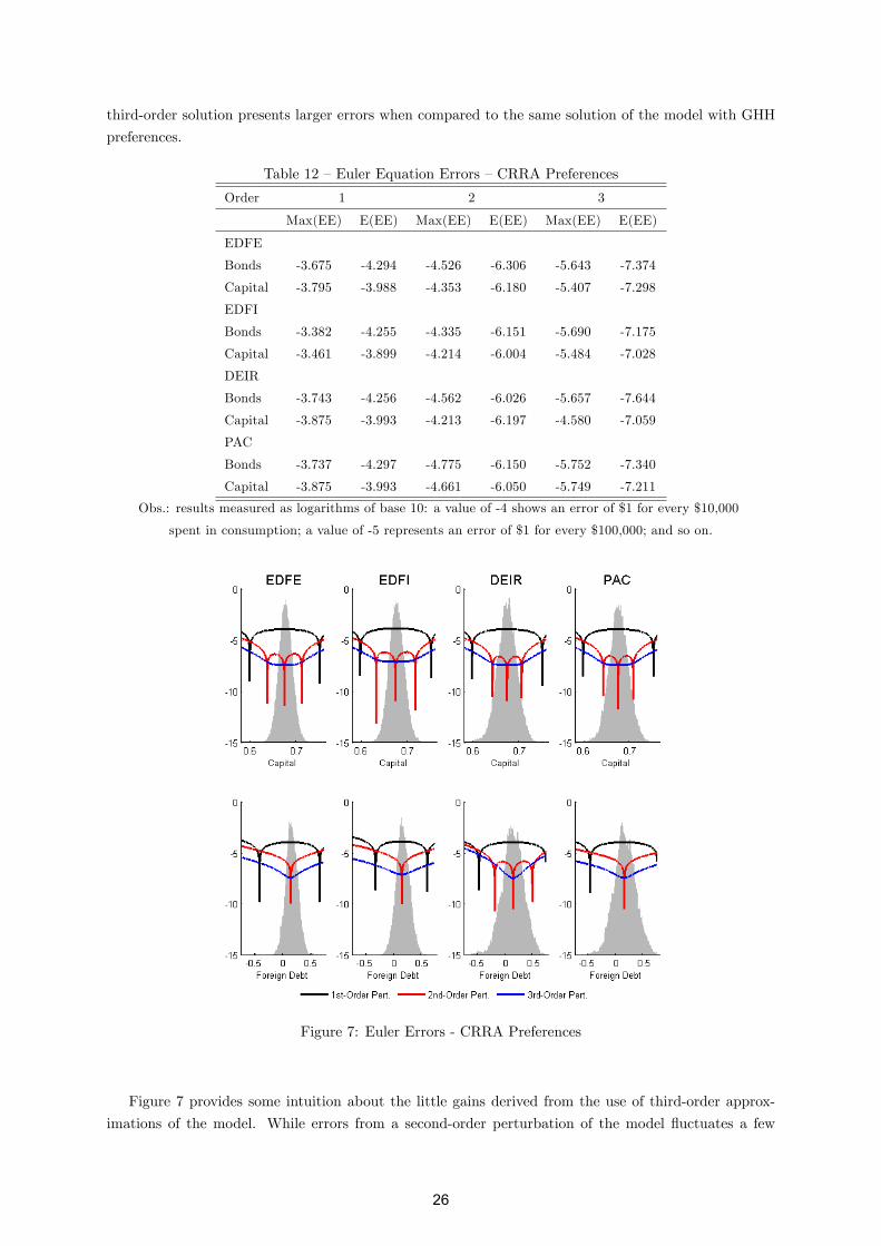
third-order solution presents larger errors when compared to the same solution of the model with GHH
preferences.
Table 12 �Euler Equation Errors �CRRA Preferences
Order 1 2 3
Max(EE) E(EE) Max(EE) E(EE) Max(EE) E(EE)
EDFE
Bonds -3.675 -4.294 -4.526 -6.306 -5.643 -7.374
Capital -3.795 -3.988 -4.353 -6.180 -5.407 -7.298
EDFI
Bonds -3.382 -4.255 -4.335 -6.151 -5.690 -7.175
Capital -3.461 -3.899 -4.214 -6.004 -5.484 -7.028
DEIR
Bonds -3.743 -4.256 -4.562 -6.026 -5.657 -7.644
Capital -3.875 -3.993 -4.213 -6.197 -4.580 -7.059
PAC
Bonds -3.737 -4.297 -4.775 -6.150 -5.752 -7.340
Capital -3.875 -3.993 -4.661 -6.050 -5.749 -7.211
Obs.: results measured as logarithms of base 10: a value of -4 shows an error of $1 for every $10,000
spent in consumption; a value of -5 represents an error of $1 for every $100,000; and so on.
Figure 7: Euler Errors - CRRA Preferences
Figure 7 provides some intuition about the little gains derived from the use of third-order approx-
imations of the model. While errors from a second-order perturbation of the model �uctuates a few
26
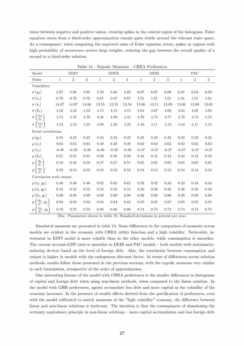
times between negative and positive values, creating spikes in the central region of the histogram, Euler
equation errors from a third-order approximation remain quite stable around the relevant state space.
As a consequence, when computing the expected value of Euler equation errors, spikes in regions with
high probability of occurrence receive large weights, reducing the gap between the overall quality of a
second to a third-order solution.
Table 13 �Ergodic Moments �CRRA Preferences
Model EDFI EDFE DEIR PAC
Order 1 2 3 1 2 3 1 2 3 1 2 3
Volatilities
� (yt) 5.97 5.96 5.95 5.70 5.68 5.68 6.07 6.07 6.06 6.07 6.04 6.03
� (ct) 0.76 0.76 0.76 0.87 0.87 0.87 1.01 1.01 1.01 1.01 1.01 1.01
� (it) 14.07 14.07 14.06 12.55 12.55 12.54 13.06 13.11 13.09 13.06 13.06 13.05
� (ht) 4.52 4.52 4.52 4.15 4.15 4.15 4.64 4.67 4.66 4.64 4.63 4.63
��tbtyt
�4.75 4.76 4.79 4.38 4.39 4.41 4.70 4.75 4.77 4.70 4.72 4.75
��catyt
�4.52 4.53 4.55 4.20 4.20 4.22 4.10 4.11 4.13 4.10 4.11 4.13
Serial correlations
� (yt) 0.25 0.25 0.25 0.23 0.23 0.23 0.32 0.33 0.33 0.32 0.32 0.32
� (ct) 0.64 0.63 0.64 0.49 0.49 0.49 0.62 0.63 0.63 0.62 0.62 0.62
� (it) -0.39 -0.39 -0.39 -0.39 -0.39 -0.39 -0.37 -0.37 -0.37 -0.37 -0.37 -0.37
� (ht) 0.31 0.31 0.31 0.29 0.29 0.29 0.44 0.44 0.44 0.44 0.43 0.43
��tbtyt
�0.58 0.58 0.58 0.57 0.57 0.57 0.65 0.65 0.65 0.65 0.65 0.65
��catyt
�0.53 0.53 0.53 0.53 0.53 0.53 0.54 0.54 0.54 0.54 0.54 0.54
Correlation with output
� (ct; yt) 0.46 0.46 0.46 0.62 0.62 0.62 0.33 0.32 0.33 0.33 0.34 0.34
� (it; yt) 0.52 0.52 0.52 0.52 0.52 0.52 0.56 0.56 0.56 0.56 0.56 0.56
� (ht; yt) 0.99 0.99 0.99 0.99 0.99 0.99 0.99 0.99 0.99 0.99 0.99 0.99
��tbtyt; yt
�0.83 0.83 0.83 0.84 0.84 0.84 0.85 0.85 0.85 0.85 0.85 0.85
��catyt; yt
�0.78 0.78 0.78 0.80 0.80 0.80 0.74 0.74 0.74 0.74 0.74 0.75
Obs.: Parameters shown in table 10. Standard-deviations in percent per year.
Simulated moments are presented in table 13. Some di¤erences in the comparison of moments across
models are evident in the economy with CRRA utility function and a high volatility. Noticeably, in-
vestment in EDFI model is more volatile than in the other models, while consumption is smoother.
The current account-GDP ratio is smoother in DEIR and PAC models �both models with stationarity-
inducing devices based on the level of foreign debt. Also, the correlation between consumption and
output is higher in models with the endogenous discount factor. In terms of di¤erences across solution
methods, results follow those presented in the previous sections, with the ergodic moments very similar
in each formulation, irrespective of the order of approximation.
One interesting feature of the model with CRRA preferences is the smaller di¤erences in histograms
of capital and foreign debt when using non-linear methods, when compared to the linear solution. In
the model with GHH preferences, agents accumulate less debt and more capital as the volatility of the
economy increases. In the presence of wealth e¤ects derived from the speci�cation of preferences, even
with the model calibrated to match moments of the "high volatility" economy, the di¤erence between
linear and non-linear solutions is irrelevant. The intuition is that the consequences of abandoning the
certainty equivalence principle in non-linear solutions �more capital accumulation and less foreign debt
27
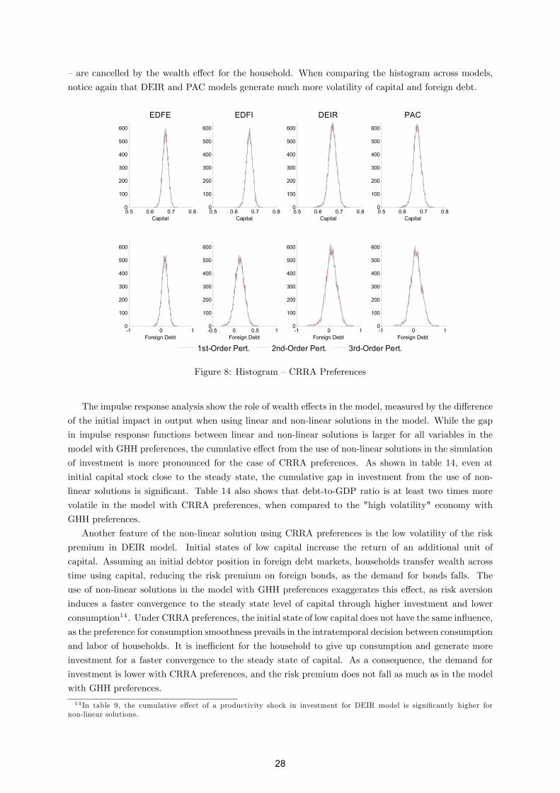
�are cancelled by the wealth e¤ect for the household. When comparing the histogram across models,
notice again that DEIR and PAC models generate much more volatility of capital and foreign debt.
0.5 0.6 0.7 0.80
100
200
300
400
500
600
Capital
EDFE
-1 0 10
100
200
300
400
500
600
Foreign Debt
0.5 0.6 0.7 0.80
100
200
300
400
500
600
Capital
EDFI
-0.5 0 0.5 10
100
200
300
400
500
600
Foreign Debt
0.5 0.6 0.7 0.80
100
200
300
400
500
600
Capital
DEIR
-1 0 10
100
200
300
400
500
600
Foreign Debt
0.5 0.6 0.7 0.80
100
200
300
400
500
600
Capital
PAC
-1 0 10
100
200
300
400
500
600
Foreign Debt
1st-Order Pert. 2nd-Order Pert. 3rd-Order Pert.
Figure 8: Histogram �CRRA Preferences
The impulse response analysis show the role of wealth e¤ects in the model, measured by the di¤erence
of the initial impact in output when using linear and non-linear solutions in the model. While the gap
in impulse response functions between linear and non-linear solutions is larger for all variables in the
model with GHH preferences, the cumulative e¤ect from the use of non-linear solutions in the simulation
of investment is more pronounced for the case of CRRA preferences. As shown in table 14, even at
initial capital stock close to the steady state, the cumulative gap in investment from the use of non-
linear solutions is signi�cant. Table 14 also shows that debt-to-GDP ratio is at least two times more
volatile in the model with CRRA preferences, when compared to the "high volatility" economy with
GHH preferences.
Another feature of the non-linear solution using CRRA preferences is the low volatility of the risk
premium in DEIR model. Initial states of low capital increase the return of an additional unit of
capital. Assuming an initial debtor position in foreign debt markets, households transfer wealth across
time using capital, reducing the risk premium on foreign bonds, as the demand for bonds falls. The
use of non-linear solutions in the model with GHH preferences exaggerates this e¤ect, as risk aversion
induces a faster convergence to the steady state level of capital through higher investment and lower
consumption14 . Under CRRA preferences, the initial state of low capital does not have the same in�uence,
as the preference for consumption smoothness prevails in the intratemporal decision between consumption
and labor of households. It is ine¢ cient for the household to give up consumption and generate more
investment for a faster convergence to the steady state of capital. As a consequence, the demand for
investment is lower with CRRA preferences, and the risk premium does not fall as much as in the model
with GHH preferences.
14 In table 9, the cumulative e¤ect of a productivity shock in investment for DEIR model is signi�cantly higher fornon-linear solutions.
28
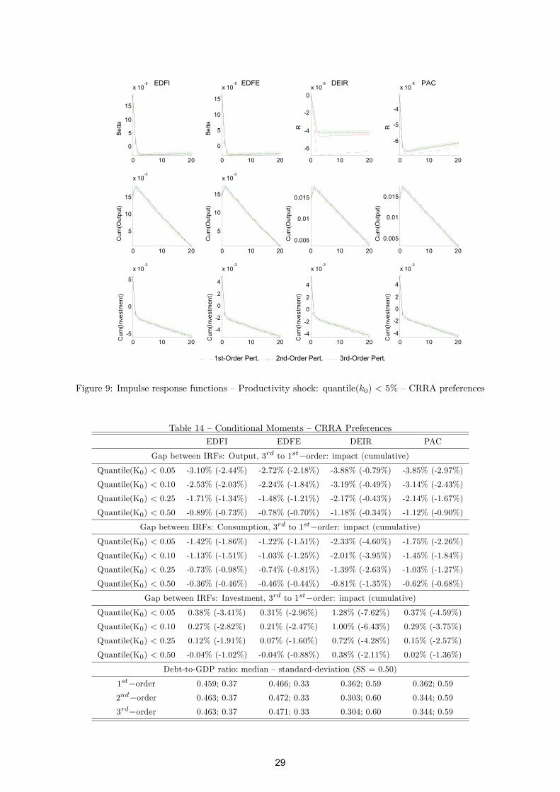
0 10 20
0
5
10
15
x 10-5 EDFI
Bet
ta
0 10 20
5
10
15
x 10-3
Cum
(Out
put)
0 10 20-5
0
5
x 10-3
Cum
(Inve
stm
ent)
0 10 20
0
5
10
15
x 10-5 EDFE
Bet
ta
0 10 20
5
10
15
x 10-3
Cum
(Out
put)
0 10 20
-4
-2
0
2
4
x 10-3
Cum
(Inve
stm
ent)
0 10 20
-6
-4
-2
0x 10
-6 DEIR
R
0 10 20
0.005
0.01
0.015
Cum
(Out
put)
0 10 20-4
-2
0
2
4
x 10-3
Cum
(Inve
stm
ent)
0 10 20
-6
-5
-4
x 10-6 PAC
R
0 10 20
0.005
0.01
0.015
Cum
(Out
put)
0 10 20-4
-2
0
2
4
x 10-3
Cum
(Inve
stm
ent)
1st-Order Pert. 2nd-Order Pert. 3rd-Order Pert.
Figure 9: Impulse response functions �Productivity shock: quantile(k0) < 5% �CRRA preferences
Table 14 �Conditional Moments �CRRA PreferencesEDFI EDFE DEIR PAC
Gap between IRFs: Output, 3rd to 1st�order: impact (cumulative)Quantile(K0) < 0.05 -3.10% (-2.44%) -2.72% (-2.18%) -3.88% (-0.79%) -3.85% (-2.97%)
Quantile(K0) < 0.10 -2.53% (-2.03%) -2.24% (-1.84%) -3.19% (-0.49%) -3.14% (-2.43%)
Quantile(K0) < 0.25 -1.71% (-1.34%) -1.48% (-1.21%) -2.17% (-0.43%) -2.14% (-1.67%)
Quantile(K0) < 0.50 -0.89% (-0.73%) -0.78% (-0.70%) -1.18% (-0.34%) -1.12% (-0.90%)
Gap between IRFs: Consumption, 3rd to 1st�order: impact (cumulative)Quantile(K0) < 0.05 -1.42% (-1.86%) -1.22% (-1.51%) -2.33% (-4.60%) -1.75% (-2.26%)
Quantile(K0) < 0.10 -1.13% (-1.51%) -1.03% (-1.25%) -2.01% (-3.95%) -1.45% (-1.84%)
Quantile(K0) < 0.25 -0.73% (-0.98%) -0.74% (-0.81%) -1.39% (-2.63%) -1.03% (-1.27%)
Quantile(K0) < 0.50 -0.36% (-0.46%) -0.46% (-0.44%) -0.81% (-1.35%) -0.62% (-0.68%)
Gap between IRFs: Investment, 3rd to 1st�order: impact (cumulative)Quantile(K0) < 0.05 0.38% (-3.41%) 0.31% (-2.96%) 1.28% (-7.62%) 0.37% (-4.59%)
Quantile(K0) < 0.10 0.27% (-2.82%) 0.21% (-2.47%) 1.00% (-6.43%) 0.29% (-3.75%)
Quantile(K0) < 0.25 0.12% (-1.91%) 0.07% (-1.60%) 0.72% (-4.28%) 0.15% (-2.57%)
Quantile(K0) < 0.50 -0.04% (-1.02%) -0.04% (-0.88%) 0.38% (-2.11%) 0.02% (-1.36%)
Debt-to-GDP ratio: median �standard-deviation (SS = 0.50)
1st�order 0.459; 0.37 0.466; 0.33 0.362; 0.59 0.362; 0.59
2nd�order 0.463; 0.37 0.472; 0.33 0.303; 0.60 0.344; 0.59
3rd�order 0.463; 0.37 0.471; 0.33 0.304; 0.60 0.344; 0.59
29
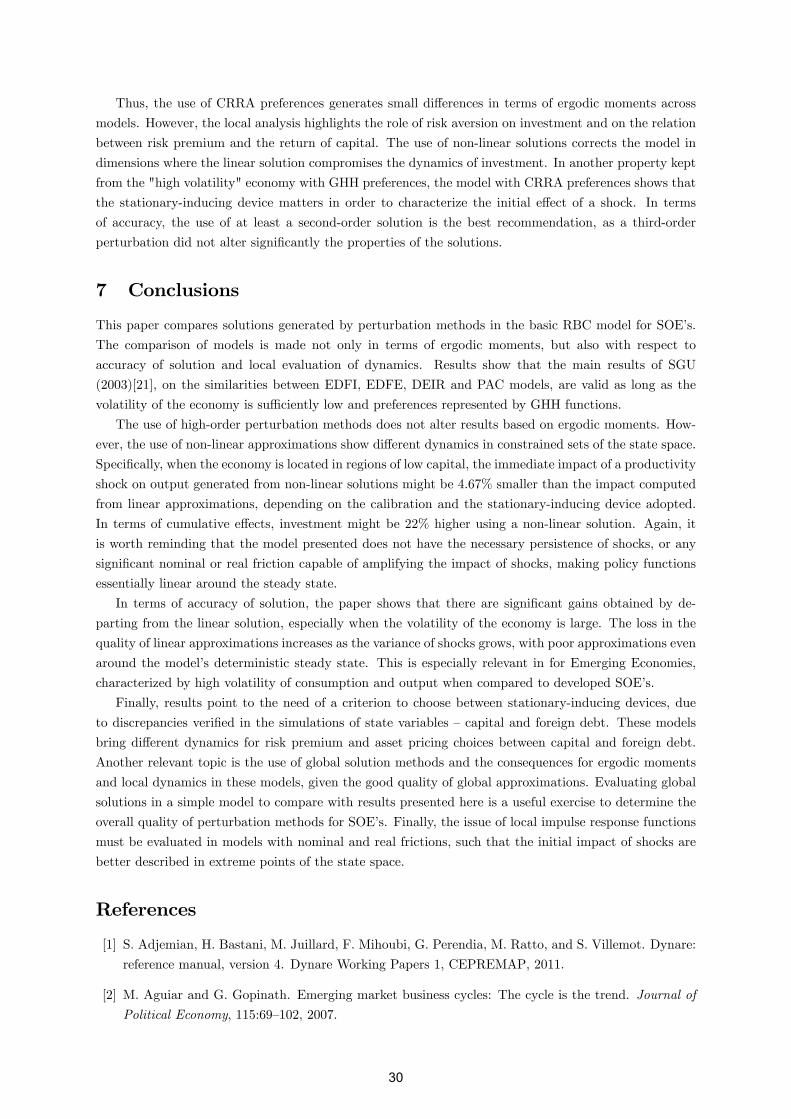
Thus, the use of CRRA preferences generates small di¤erences in terms of ergodic moments across
models. However, the local analysis highlights the role of risk aversion on investment and on the relation
between risk premium and the return of capital. The use of non-linear solutions corrects the model in
dimensions where the linear solution compromises the dynamics of investment. In another property kept
from the "high volatility" economy with GHH preferences, the model with CRRA preferences shows that
the stationary-inducing device matters in order to characterize the initial e¤ect of a shock. In terms
of accuracy, the use of at least a second-order solution is the best recommendation, as a third-order
perturbation did not alter signi�cantly the properties of the solutions.
7 Conclusions
This paper compares solutions generated by perturbation methods in the basic RBC model for SOE�s.
The comparison of models is made not only in terms of ergodic moments, but also with respect to
accuracy of solution and local evaluation of dynamics. Results show that the main results of SGU
(2003)[21], on the similarities between EDFI, EDFE, DEIR and PAC models, are valid as long as the
volatility of the economy is su¢ ciently low and preferences represented by GHH functions.
The use of high-order perturbation methods does not alter results based on ergodic moments. How-
ever, the use of non-linear approximations show di¤erent dynamics in constrained sets of the state space.
Speci�cally, when the economy is located in regions of low capital, the immediate impact of a productivity
shock on output generated from non-linear solutions might be 4.67% smaller than the impact computed
from linear approximations, depending on the calibration and the stationary-inducing device adopted.
In terms of cumulative e¤ects, investment might be 22% higher using a non-linear solution. Again, it
is worth reminding that the model presented does not have the necessary persistence of shocks, or any
signi�cant nominal or real friction capable of amplifying the impact of shocks, making policy functions
essentially linear around the steady state.
In terms of accuracy of solution, the paper shows that there are signi�cant gains obtained by de-
parting from the linear solution, especially when the volatility of the economy is large. The loss in the
quality of linear approximations increases as the variance of shocks grows, with poor approximations even
around the model�s deterministic steady state. This is especially relevant in for Emerging Economies,
characterized by high volatility of consumption and output when compared to developed SOE�s.
Finally, results point to the need of a criterion to choose between stationary-inducing devices, due
to discrepancies veri�ed in the simulations of state variables �capital and foreign debt. These models
bring di¤erent dynamics for risk premium and asset pricing choices between capital and foreign debt.
Another relevant topic is the use of global solution methods and the consequences for ergodic moments
and local dynamics in these models, given the good quality of global approximations. Evaluating global
solutions in a simple model to compare with results presented here is a useful exercise to determine the
overall quality of perturbation methods for SOE�s. Finally, the issue of local impulse response functions
must be evaluated in models with nominal and real frictions, such that the initial impact of shocks are
better described in extreme points of the state space.
References
[1] S. Adjemian, H. Bastani, M. Juillard, F. Mihoubi, G. Perendia, M. Ratto, and S. Villemot. Dynare:
reference manual, version 4. Dynare Working Papers 1, CEPREMAP, 2011.
[2] M. Aguiar and G. Gopinath. Emerging market business cycles: The cycle is the trend. Journal of
Political Economy, 115:69�102, 2007.
30
[3] E. M. Aldrich and H. Kung. Computational methods for production-based asset pricing models with
recursive utility. Economic Research Initiatives at Duke (ERID) Working Paper Series 87, Duke
University, Oct. 2009.
[4] S. An. Bayesian estimation of DSGE models: Lessons from second-order approximations. Bank for
International Settlements - BIS, June 2008.
[5] S. B. Aruoba, J. Fernández-Villaverde, and J. F. Rubio-Ramírez. Comparing solution methods for
dynamic equilibrium economies. Journal of Economic Dynamics and Control, 30(12):2477�2508,
2006.
[6] D. Caldara, J. Fernández-Villaverde, J. F. Rubio-Ramírez, and W. Yao. Computing DSGE models
with recursive preferences. NBER Working Papers 15026, National Bureau of Economic Research,
Inc, June 2009.
[7] F. Collard and M. Juillard. Accuracy of stochastic perturbation methods: The case of asset pricing
models. Journal of Economic Dynamics and Control, 25(6-7):979�999, 2001.
[8] L. G. Epstein and S. E. Zin. Substitution, risk aversion, and the temporal behavior of consumption
and asset returns: A theoretical framework. Econometrica, 57(4):937�69, 1989.
[9] J. Fernández-Villaverde, P. A. Guerrón-Quintana, J. F. Rubio-Ramírez, and M. Uribe. Risk matters:
The real e¤ects of volatility shocks. NBER Working Papers 14875, National Bureau of Economic
Research, Inc, Apr. 2009.
[10] J. Fernández-Villaverde and J. F. Rubio-Ramírez. Estimating dynamic equilibrium economies: linear
versus nonlinear likelihood. Journal of Applied Econometrics, 20(7):891�910, 2005.
[11] J. Fernández-Villaverde and J. F. Rubio-Ramírez. Solving DSGE models with perturbation methods
and a change of variables. Journal of Economic Dynamics and Control, 30(12):2509�2531, 2006.
[12] J. Greenwood, Z. Hercowitz, and G. W. Hu¤man. Investment, capacity utilization, and the real
business cycle. American Economic Review, 78(3):402�17, 1988.
[13] W. J. D. Haan and A. Marcet. Accuracy in simulations. The Review of Economic Studies, 61(1):3�17,
Jan. 1994.
[14] W. J. D. Haan and J. D. Wind. How well-behaved are higher-order perturbation solutions? DNB
Working Papers 240, Netherlands Central Bank, Research Department, Jan. 2010.
[15] K. L. Judd. Numerical methods in economics. MIT Press, 1998.
[16] O. Kamenik. DSGE models with Dynare++. A tutorial. Technical report, Jan. 2011.
[17] J. Kim, S. Kim, E. Schaumburg, and C. A. Sims. Calculating and using second-order accurate
solutions of discrete time dynamic equilibrium models. Journal of Economic Dynamics and Control,
32(11):3397�3414, Nov. 2008.
[18] G. Koop, M. H. Pesaran, and S. M. Potter. Impulse response analysis in nonlinear multivariate
models. Journal of Econometrics, 74(1):119�147, 1996.
[19] G. C. Lim and P. D. McNelis. Computational Macroeconomics for the Open Economy. The MIT
Press, Oct. 2008.
31

[20] E. G. Mendoza. Real business cycles in a small open economy. American Economic Review,
81(4):797�818, 1991.
[21] S. Schmitt-Grohé and M. Uribe. Closing small open economy models. Journal of International
Economics, 61(1):163�185, Oct. 2003.
[22] H. D. Seoane. Nonlinear solution methods�implications for small open economy models. Manuscript,
Duke University, Jan. 2011.
[23] M. Shamloo and A. Malkhozov. Asset prices in a¢ ne real business cycle models. IMF Working
Papers 10/249, International Monetary Fund, Nov. 2010.
32
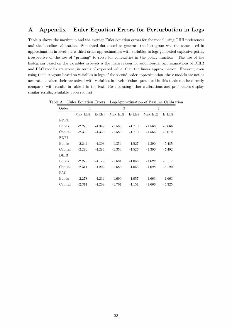
A Appendix �Euler Equation Errors for Perturbation in Logs
Table A shows the maximum and the average Euler equation errors for the model using GHH preferences
and the baseline calibration. Simulated data used to generate the histogram was the same used in
approximation in levels, as a third-order approximation with variables in logs generated explosive paths,
irrespective of the use of "pruning" to solve for convexities in the policy function. The use of the
histogram based on the variables in levels is the main reason for second-order approximations of DEIR
and PAC models are worse, in terms of expected value, than the linear approximation. However, even
using the histogram based on variables in logs of the second-order approximation, these models are not as
accurate as when their are solved with variables in levels. Values presented in this table can be directly
compared with results in table 4 in the text. Results using other calibrations and preferences display
similar results, available upon request.
Table A �Euler Equation Errors �Log-Approximation of Baseline Calibration
Order 1 2 3
Max(EE) E(EE) Max(EE) E(EE) Max(EE) E(EE)
EDFE
Bonds -2.273 -4.349 -1.583 -4.710 -1.566 -5.666
Capital -2.309 -4.336 -1.583 -4.710 -1.566 -5.672
EDFI
Bonds -2.244 -4.303 -1.354 -4.527 -1.390 -5.485
Capital -2.296 -4.284 -1.354 -4.526 -1.390 -5.492
DEIR
Bonds -2.279 -4.179 -1.681 -4.053 -1.622 -5.117
Capital -2.311 -4.202 -1.686 -4.055 -1.628 -5.129
PAC
Bonds -2.278 -4.234 -1.699 -4.057 -1.663 -4.663
Capital -2.311 -4.209 -1.701 -4.151 -1.666 -5.325
33
Banco Central do Brasil
Trabalhos para Discussão Os Trabalhos para Discussão do Banco Central do Brasil estão disponíveis para download no website
http://www.bcb.gov.br/?TRABDISCLISTA
Working Paper Series
The Working Paper Series of the Central Bank of Brazil are available for download at http://www.bcb.gov.br/?WORKINGPAPERS
221 Financial Instability and Credit Constraint: evidence from the cost of
bank financing Bruno S. Martins
Nov/2010
222 O Comportamento Cíclico do Capital dos Bancos Brasileiros R. A. Ferreira, A. C. Noronha, B. M. Tabak e D. O. Cajueiro
Nov/2010
223 Forecasting the Yield Curve with Linear Factor Models Marco Shinobu Matsumura, Ajax Reynaldo Bello Moreira and José Valentim Machado Vicente
Nov/2010
224 Emerging Floaters: pass-throughs and (some) new commodity currencies Emanuel Kohlscheen
Nov/2010
225 Expectativas Inflacionárias e Inflação Implícita no Mercado Brasileiro Flávio de Freitas Val, Claudio Henrique da Silveira Barbedo e Marcelo Verdini Maia
Nov/2010
226 A Macro Stress Test Model of Credit Risk for the Brazilian Banking Sector Francisco Vazquez, Benjamin M.Tabak and Marcos Souto
Nov/2010
227 Uma Nota sobre Erros de Previsão da Inflação de Curto Prazo Emanuel Kohlscheen
Nov/2010
228 Forecasting Brazilian Inflation Using a Large Data Set Francisco Marcos Rodrigues Figueiredo
Dec/2010
229 Financial Fragility in a General Equilibrium Model: the Brazilian case Benjamin M. Tabak, Daniel O. Cajueiro and Dimas M. Fazio
Dec/2010
230 Is Inflation Persistence Over? Fernando N. de Oliveira and Myrian Petrassi
Dec/2010
231 Capital Requirements and Business Cycles with Credit Market Imperfections P. R. Agénor, K. Alper and L. Pereira da Silva
Jan/2011
232 Modeling Default Probabilities: the case of Brazil Benjamin M. Tabak, Daniel O. Cajueiro and A. Luduvice
Jan/2011
34
233 Emerging Floaters: pass-throughs and (some) new commodity currencies Emanuel Kohlscheen
Jan/2011
234 Cyclical Effects of Bank Capital Requirements with Imperfect Credit Markets Pierre-Richard Agénor and Luiz A. Pereira da Silva
Jan/2011
235 Revisiting bank pricing policies in Brazil: Evidence from loan and deposit markets Leonardo S. Alencar
Mar/2011
236 Optimal costs of sovereign default Leonardo Pio Perez
Apr/2011
237 Capital Regulation, Monetary Policy and Financial Stability P.R. Agénor, K. Alper, and L. Pereira da Silva
Apr/2011
238 Choques não Antecipados de Política Monetária e a Estrutura a Termo das Taxas de Juros no Brasil Fernando N. de Oliveira e Leonardo Ramos
Abr/2011
239 SAMBA: Stochastic Analytical Model with a Bayesian Approach Marcos R. de Castro, Solange N. Gouvea, André Minella, Rafael C. Santos and Nelson F. Souza-Sobrinho
Apr/2011
240 Fiscal Policy in Brazil through the Lens of an Estimated DSGE Model Fabia A. de Carvalho and Marcos Valli
Apr/2011
241 Macro Stress Testing of Credit Risk Focused on the Tails Ricardo Schechtman and Wagner Piazza Gaglianone
May/2011
242 Determinantes do Spread Bancário Ex-Post no Mercado Brasileiro José Alves Dantas, Otávio Ribeiro de Medeiros e Lúcio Rodrigues Capelletto
Maio/2011
243 Economic Activity and Financial Institutional Risk: an empirical analysis for the Brazilian banking industry Helder Ferreira de Mendonça, Délio José Cordeiro Galvão and Renato Falci Villela Loures
May/2011
244 Profit, Cost and Scale Eficiency for Latin American Banks: concentration-performance relationship Benjamin M. Tabak, Dimas M. Fazio and Daniel O. Cajueiro
May/2011
245 Pesquisa Trimestral de Condições de Crédito no Brasil Clodoaldo Aparecido Annibal e Sérgio Mikio Koyama
Jun/2011
246 Impacto do Sistema Cooperativo de Crédito na Eficiência do Sistema Financeiro Nacional Michel Alexandre da Silva
Ago/2011
247 Forecasting the Yield Curve for the Euro Region Benjamim M. Tabak, Daniel O. Cajueiro and Alexandre B. Sollaci
Aug/2011
248 Financial regulation and transparency of information: first steps on new land Helder Ferreira de Mendonça, Délio José Cordeiro Galvão and Renato Falci Villela Loures
Aug/2011
35
249 Directed clustering coefficient as a measure of systemic risk in complex banking networks B. M. Tabak, M. Takami, J. M. C. Rocha and D. O. Cajueiro
Aug/2011
250 Recolhimentos Compulsórios e o Crédito Bancário Brasileiro
Paulo Evandro Dawid e Tony Takeda
Ago/2011
251 Um Exame sobre como os Bancos Ajustam seu Índice de Basileia no Brasil Leonardo S. Alencar
Ago/2011
252 Comparação da Eficiência de Custo para BRICs e América Latina Lycia M. G. Araujo, Guilherme M. R. Gomes, Solange M. Guerra e Benjamin M. Tabak
Set/2011
253 Bank Efficiency and Default in Brazil: causality tests Benjamin M. Tabak, Giovana L. Craveiro and Daniel O. Cajueiro
Oct/2011
254 Macroprudential Regulation and the Monetary Transmission Mechanism Pierre-Richard Agénor and Luiz A. Pereira da Silva
Nov/2011
255 An Empirical Analysis of the External Finance Premium of Public Non-Financial Corporations in Brazil Fernando N. de Oliveira and Alberto Ronchi Neto
Nov/2011
256 The Self-insurance Role of International Reserves and the 2008-2010 Crisis Antonio Francisco A. Silva Jr
Nov/2011
257 Cooperativas de Crédito: taxas de juros praticadas e fatores de viabilidade Clodoaldo Aparecido Annibal e Sérgio Mikio Koyama
Nov/2011
258 Bancos Oficiais e Crédito Direcionado – O que diferencia o mercado de crédito brasileiro? Eduardo Luis Lundberg
Nov/2011
259 The impact of monetary policy on the exchange rate: puzzling evidence from three emerging economies Emanuel Kohlscheen
Nov/2011
260 Credit Default and Business Cycles: an empirical investigation of Brazilian retail loans Arnildo da Silva Correa, Jaqueline Terra Moura Marins, Myrian Beatriz Eiras das Neves and Antonio Carlos Magalhães da Silva
Nov/2011
261 The relationship between banking market competition and risk-taking: do size and capitalization matter? Benjamin M. Tabak, Dimas M. Fazio and Daniel O. Cajueiro
Nov/2011
36