The Accelerator Hamiltonian in a Curved Coordinate … · The Accelerator Hamiltonian in a Curved...
17
Linear Dynamics, Lecture 3 The Accelerator Hamiltonian in a Curved Coordinate System Andy Wolski University of Liverpool, and the Cockcroft Institute, Daresbury, UK. November, 2012 What we Learned in the Previous Lecture In the previous lecture, we derived a Hamiltonian for the motion of a particle through an electromagnetic field, with dynamical variables appropriate for a particle accelerator. For particles close to the reference trajectory, and with energy close to the reference energy, the values of the dynamical variables are expected to remain small as the particle moves through the accelerator. Since the dynamical variables take small values, we can make approximations to the Hamiltonian to construct linear maps. We saw how this could be applied to the map for a field-free region (a drift space ). So far we have assumed that the reference trajectory is a straight line. Linear Dynamics, Lecture 3 1 Curved Coordinate Systems
Transcript of The Accelerator Hamiltonian in a Curved Coordinate … · The Accelerator Hamiltonian in a Curved...
Linear Dynamics, Lecture 3
The Accelerator Hamiltonian in a Curved
Coordinate System
Andy Wolski
University of Liverpool, and the Cockcroft Institute, Daresbury, UK.
November, 2012
What we Learned in the Previous Lecture
In the previous lecture, we derived a Hamiltonian for the
motion of a particle through an electromagnetic field, with
dynamical variables appropriate for a particle accelerator. For
particles close to the reference trajectory, and with energy close
to the reference energy, the values of the dynamical variables
are expected to remain small as the particle moves through the
accelerator.
Since the dynamical variables take small values, we can make
approximations to the Hamiltonian to construct linear maps.
We saw how this could be applied to the map for a field-free
region (a drift space).
So far we have assumed that the reference trajectory is a
straight line.
Linear Dynamics, Lecture 3 1 Curved Coordinate Systems
Course Outline
Part I (Lectures 1 – 5): Dynamics of a relativistic charged
particle in the electromagnetic field of an accelerator beamline.
1. Review of Hamiltonian mechanics
2. The accelerator Hamiltonian in a straight coordinate
system
3. The Hamiltonian for a relativistic particle in a general
electromagnetic field using accelerator coordinates
4. Dynamical maps for linear elements
5. Three loose ends: edge focusing; chromaticity; beam
rigidity.
Linear Dynamics, Lecture 3 2 Curved Coordinate Systems
Goals of This Lecture
In this lecture, we shall see how to modify the Hamiltonian to
deal with cases where the reference trajectory is curved. This
will allow us to deal with dipole magnets, where all particles
follow curved paths.
Using a curved reference trajectory in dipole magnets allows us
to maintain small values for the dynamical variables, even
where the deflection from the dipole is large. This means we
can continue to use series expansion approximations for the
Hamiltonian in such cases.
Ultimately, we shall derive the linear transfer map (transfer
matrix) for a dipole.
Linear Dynamics, Lecture 3 3 Curved Coordinate Systems
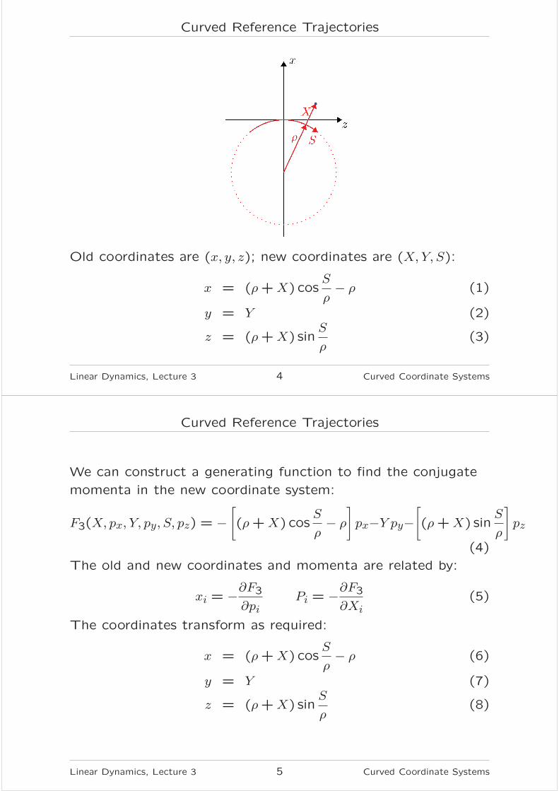
Curved Reference Trajectories
Old coordinates are (x, y, z); new coordinates are (X,Y, S):
x = (ρ+X) cosS
ρ− ρ (1)
y = Y (2)
z = (ρ+X) sinS
ρ(3)
Linear Dynamics, Lecture 3 4 Curved Coordinate Systems
Curved Reference Trajectories
We can construct a generating function to find the conjugate
momenta in the new coordinate system:
F3(X, px, Y, py, S, pz) = −
[
(ρ+X) cosS
ρ− ρ
]
px−Y py−
[
(ρ+X) sinS
ρ
]
pz
(4)
The old and new coordinates and momenta are related by:
xi = −∂F3
∂piPi = −
∂F3
∂Xi(5)
The coordinates transform as required:
x = (ρ+X) cosS
ρ− ρ (6)
y = Y (7)
z = (ρ+X) sinS
ρ(8)
Linear Dynamics, Lecture 3 5 Curved Coordinate Systems
Curved Reference Trajectories
The new transverse momenta are given by:
PX = px cosS
ρ+ pz sin
S
ρ(9)
PY = py (10)
Linear Dynamics, Lecture 3 6 Curved Coordinate Systems
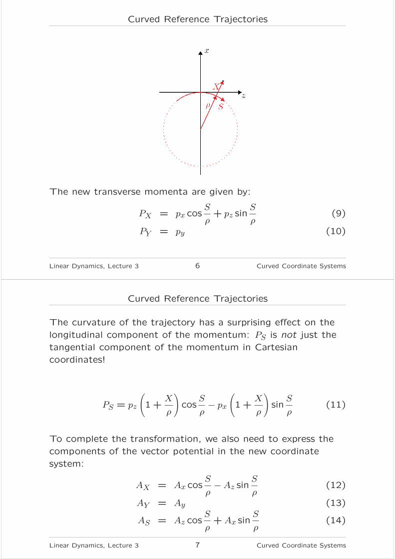
Curved Reference Trajectories
The curvature of the trajectory has a surprising effect on the
longitudinal component of the momentum: PS is not just the
tangential component of the momentum in Cartesian
coordinates!
PS = pz
(
1+X
ρ
)
cosS
ρ− px
(
1+X
ρ
)
sinS
ρ(11)
To complete the transformation, we also need to express the
components of the vector potential in the new coordinate
system:
AX = Ax cosS
ρ−Az sin
S
ρ(12)
AY = Ay (13)
AS = Az cosS
ρ+Ax sin
S
ρ(14)
Linear Dynamics, Lecture 3 7 Curved Coordinate Systems
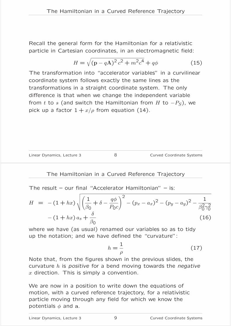
The Hamiltonian in a Curved Reference Trajectory
Recall the general form for the Hamiltonian for a relativistic
particle in Cartesian coordinates, in an electromagnetic field:
H =√
(p− qA)2 c2 +m2c4 + qφ (15)
The transformation into “accelerator variables” in a curvilinear
coordinate system follows exactly the same lines as the
transformations in a straight coordinate system. The only
difference is that when we change the independent variable
from t to s (and switch the Hamiltonian from H to −PS), we
pick up a factor 1 + x/ρ from equation (14).
Linear Dynamics, Lecture 3 8 Curved Coordinate Systems
The Hamiltonian in a Curved Reference Trajectory
The result – our final “Accelerator Hamiltonian” – is:
H = − (1 + hx)
√
√
√
√
(
1
β0+ δ −
qφ
P0c
)2
− (px − ax)2− (py − ay)
2−
1
β20γ
20
− (1 + hx) as +δ
β0(16)
where we have (as usual) renamed our variables so as to tidy
up the notation; and we have defined the “curvature”:
h =1
ρ(17)
Note that, from the figures shown in the previous slides, the
curvature h is positive for a bend moving towards the negative
x direction. This is simply a convention.
We are now in a position to write down the equations of
motion, with a curved reference trajectory, for a relativistic
particle moving through any field for which we know the
potentials φ and a.
Linear Dynamics, Lecture 3 9 Curved Coordinate Systems
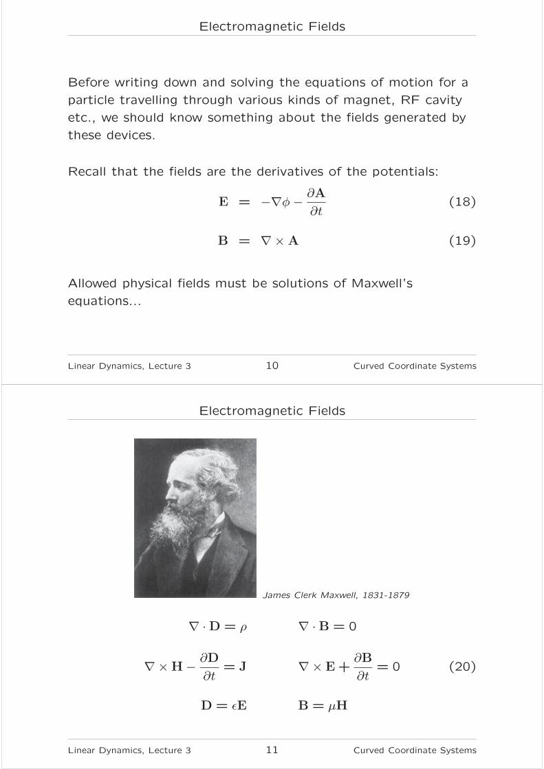
Electromagnetic Fields
Before writing down and solving the equations of motion for a
particle travelling through various kinds of magnet, RF cavity
etc., we should know something about the fields generated by
these devices.
Recall that the fields are the derivatives of the potentials:
E = −∇φ−∂A
∂t(18)
B = ∇×A (19)
Allowed physical fields must be solutions of Maxwell’s
equations...
Linear Dynamics, Lecture 3 10 Curved Coordinate Systems
Electromagnetic Fields
James Clerk Maxwell, 1831-1879
∇ ·D = ρ ∇ ·B = 0
∇×H−∂D
∂t= J ∇× E+
∂B
∂t= 0 (20)
D = εE B = µH
Linear Dynamics, Lecture 3 11 Curved Coordinate Systems

Magnetic Multipole Fields
Finding solutions to Maxwell’s equations for a given set of
boundary conditions is in general no easy task. Significant
effort has been devoted to developing computer codes to solve
this problem accurately and efficiently. Such codes have many
important applications in accelerator physics.
Fortunately, for linear beam dynamics, we are interested in a
few simple cases. In particular, we note that we can write the
field in a “long straight multipole” magnet as:
By + iBx =∞∑
n=1
(bn + ian)
(
x+ iy
r0
)n−1
(21)
where bn and an are arbitrary coefficients (chosen to give the
correct field map), and r0 is an arbitrary “reference radius”. It
is readily shown that the field of (21) satisfies Maxwell’s
equations (20).
Linear Dynamics, Lecture 3 12 Curved Coordinate Systems
Magnetic Multipole Fields
The magnetic multipole field expansion is:
By + iBx =∞∑
n=1
(bn + ian)
(
x+ iy
r0
)n−1
(22)
The “multipole components” are indexed by the value of n: so
n = 1 is a dipole; n = 2 is a quadrupole; n = 3 is a sextupole,
etc.
An ideal multipole has coefficients an and bn equal to zero, for
all except one value of n.
A “normal multipole” has an = 0 for all values of n; a “skew”
multipole has bn = 0 for all values of n.
Linear Dynamics, Lecture 3 13 Curved Coordinate Systems
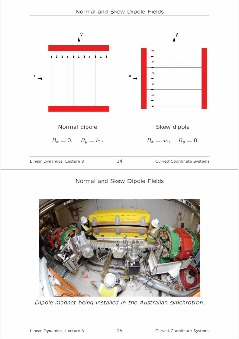
Normal and Skew Dipole Fields
Normal dipole Skew dipole
Bx = 0, By = b1. Bx = a1, By = 0.
Linear Dynamics, Lecture 3 14 Curved Coordinate Systems
Normal and Skew Dipole Fields
Dipole magnet being installed in the Australian synchrotron.
Linear Dynamics, Lecture 3 15 Curved Coordinate Systems
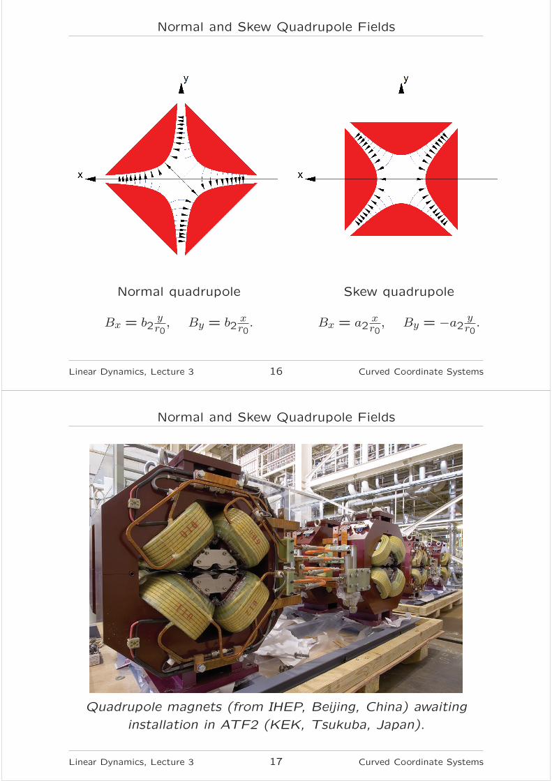
Normal and Skew Quadrupole Fields
Normal quadrupole Skew quadrupole
Bx = b2yr0, By = b2
xr0. Bx = a2
xr0, By = −a2
yr0.
Linear Dynamics, Lecture 3 16 Curved Coordinate Systems
Normal and Skew Quadrupole Fields
Quadrupole magnets (from IHEP, Beijing, China) awaiting
installation in ATF2 (KEK, Tsukuba, Japan).
Linear Dynamics, Lecture 3 17 Curved Coordinate Systems

Normal and Skew Sextupole Fields
Normal sextupole Skew sextupole
Bx = 2b3xyr20, By = b3
x2−y2
r20. Bx = a3
x2−y2
r20, By = −2a3
xyr20.
Linear Dynamics, Lecture 3 18 Curved Coordinate Systems
Normal and Skew Sextupole Fields
Sextupole magnet from the ATF (KEK, Tsukuba, Japan).
Linear Dynamics, Lecture 3 19 Curved Coordinate Systems
Magnetic Vector Potential for Multipole Fields
Let us write down the magnetic vector potential:
Ax = 0, Ay = 0, Az = −<
∞∑
n=1
(bn + ian)(x+ iy)n
nrn−10
(23)
We find from the standard relation between the magnetic field
and the vector potential:
B = ∇×A (24)
that the potential (23) gives the magnetic multipole field (22):
By + iBx = −∂Az
∂x+ i
∂Az
∂y=
∞∑
n=1
(bn + ian)
(
x+ iy
r0
)n−1
(25)
Although there are many possible vector potentials that give
the same field (25) (and all give the same equations of
motion!) the particular choice (23), is convenient, because the
transverse components are zero, and there is no dependence on
the longitudinal coordinate.
Linear Dynamics, Lecture 3 20 Curved Coordinate Systems
Magnetic Vector Potential for a Dipole Field
Let’s consider first the dipole field. This should be easy: it’s
just a uniform field perpendicular to the reference trajectory.
But there’s a catch...
... a dipole field will lead to a curved trajectory for the
reference particle. In other words, we will need to use a curved
reference trajectory, so when writing down the magnetic vector
potential A, we have to take into account the fact we are using
curvilinear coordinates.
Our vector potential should satisfy:
B = ∇×A (26)
with
Bx = 0, By = B0, Bs = 0 (27)
Linear Dynamics, Lecture 3 21 Curved Coordinate Systems
Vector Calculus in Orthogonal Curvilinear Coordinates
In general curvilinear coordinates (q1, q2, q3), the curl of a vector
field can be written:
[∇×A]1 =1
Q2Q3
(
∂
∂q2Q3A3 −
∂
∂q3Q2A2
)
(28)
[∇×A]2 =1
Q3Q1
(
∂
∂q3Q1A1 −
∂
∂q1Q3A3
)
(29)
[∇×A]3 =1
Q1Q2
(
∂
∂q1Q2A2 −
∂
∂q2Q1A1
)
(30)
where
Q2i =
(
∂x
∂qi
)2
+
(
∂y
∂qi
)2
+
(
∂z
∂qi
)2
(31)
Linear Dynamics, Lecture 3 22 Curved Coordinate Systems
Magnetic Vector Potential for a Dipole Field
In our coordinates (1), (2), (3), we find that the curl is given
by:
[∇×A]x =∂As
∂y−
1
(1 + hx)
∂Ay
∂s(32)
[∇×A]y =1
(1+ hx)
∂Ax
∂s−
h
(1 + hx)As −
∂As
∂x(33)
[∇×A]s =∂Ay
∂x−
∂Ax
∂y(34)
Using these expressions we find that the vector potential in our
curvilinear coordinates:
Ax = 0 Ay = 0 As = −B0
(
x−hx2
2(1 + hx)
)
(35)
gives the magnetic field:
Bx = 0 By = B0 Bs = 0 (36)
as desired.
Linear Dynamics, Lecture 3 23 Curved Coordinate Systems

Hamiltonian for a Dipole Field
Using the vector potential (35), and the general accelerator
Hamiltonian (16) we construct the Hamiltonian for a dipole:
H =δ
β0− (1 + hx)
√
√
√
√
(
1
β0+ δ
)2
− p2x − p2y −1
β20γ
20
+(1+ hx) k0
(
x−hx2
2(1 + hx)
)
(37)
Note that the normalised dipole field strength is given by:
k0 =q
P0B0 (38)
where q is the charge of the reference particle, and P0 is the
reference momentum.
Linear Dynamics, Lecture 3 24 Curved Coordinate Systems
Hamiltonian for a Dipole Field
The full Hamiltonian for a dipole (37) looks rather intimidating.
We shall resort to the same technique we used to get a linear
map for a drift space, and expand the Hamiltonian to
second-order in the dynamical variables. As before, this is valid
as long as the dynamical variables remain small.
The second-order Hamiltonian is:
H2 =1
2p2x +
1
2p2y + (k0 − h)x+
1
2hk0x
2−
h
β0xδ −
δ2
2β20γ
20
(39)
We can tell a good deal already just by looking at this
Hamiltonian...
Linear Dynamics, Lecture 3 25 Curved Coordinate Systems

Hamiltonian for a Dipole Field
The second-order Hamiltonian is (39):
H2 =1
2p2x +
1
2p2y + (k0 − h)x+
1
2hk0x
2−
h
β0xδ +
δ2
2β20γ
20
(40)
Note the term (k0 − h)x. A term in the Hamiltonian that is first
order in one of the variables results in a zeroth-order term in
the map for the conjugate variable. In this case, we expect to
see a horizontal deflection – a change in px. This happens if
the curvature of the reference trajectory is not matched to the
magnetic field of the dipole. If k0 = h, then the curvature is
properly matched, and this term vanishes: a particle initially on
the reference trajectory and having the reference energy stays
on the reference trajectory through the dipole.
Linear Dynamics, Lecture 3 26 Curved Coordinate Systems
Hamiltonian for a Dipole Field
The second-order Hamiltonian is (39):
H2 =1
2p2x +
1
2p2y + (k0 − h)x+
1
2hk0x
2−
h
β0xδ +
δ2
2β20γ
20
(41)
Next, note the term 12hk0x
2. This looks like a “focusing term”
– recall the potential energy term in the Hamiltonian for an
harmonic oscillator. It appears that in moving through the
dipole, particles will oscillate about the reference trajectory.
This is perhaps unexpected. How do we understand this effect?
Linear Dynamics, Lecture 3 27 Curved Coordinate Systems
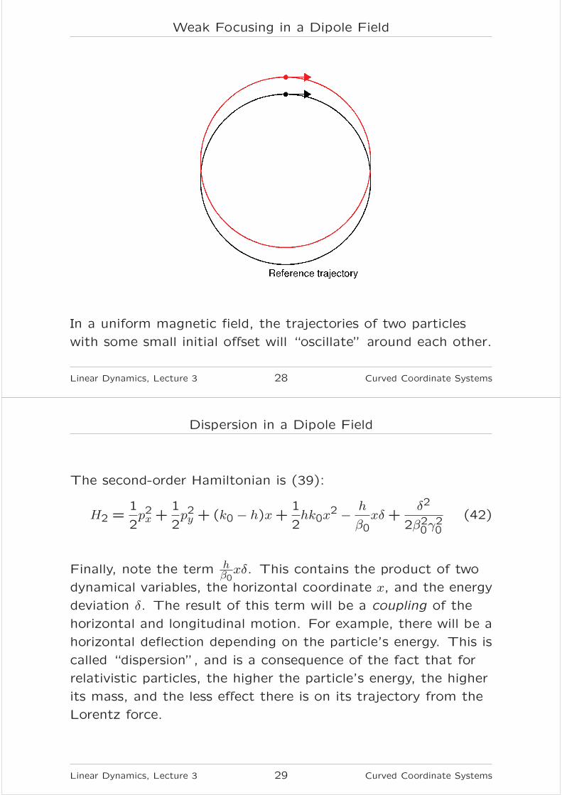
Weak Focusing in a Dipole Field
In a uniform magnetic field, the trajectories of two particles
with some small initial offset will “oscillate” around each other.
Linear Dynamics, Lecture 3 28 Curved Coordinate Systems
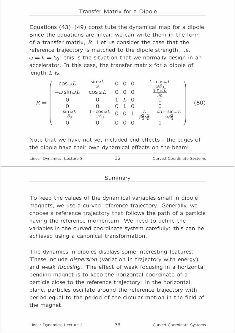
Dispersion in a Dipole Field
The second-order Hamiltonian is (39):
H2 =1
2p2x +
1
2p2y + (k0 − h)x+
1
2hk0x
2−
h
β0xδ +
δ2
2β20γ
20
(42)
Finally, note the term hβ0
xδ. This contains the product of two
dynamical variables, the horizontal coordinate x, and the energy
deviation δ. The result of this term will be a coupling of the
horizontal and longitudinal motion. For example, there will be a
horizontal deflection depending on the particle’s energy. This is
called “dispersion”, and is a consequence of the fact that for
relativistic particles, the higher the particle’s energy, the higher
its mass, and the less effect there is on its trajectory from the
Lorentz force.
Linear Dynamics, Lecture 3 29 Curved Coordinate Systems

Dynamical Map for a Dipole
Now we have the Hamiltonian for a dipole, and have considered
some of the dynamics we are likely to expect from it. What are
the solutions to the equations of motion?
Hamilton’s equations following from the Hamiltonian (39) are
essentially those for an harmonic oscillator. In the horizontal
plane, the solutions are:
x(s) = x(0) cosωs+ px(0)sinωs
ω+
(
δ(0)h
β0+ h− k0
)
(1− cosωs)
ω2
(43)
px(s) = −x(0)ω sinωs+ px(0) cosωs+
(
δ(0)h
β0+ h− k0
)
sinωs
ω
(44)
where:
ω =√
hk0 (45)
Linear Dynamics, Lecture 3 30 Curved Coordinate Systems
Dynamical Map for a Dipole
In the vertical plane, the solutions are:
y(s) = y(0) + py(0)s (46)
py(s) = py(0) (47)
which is the same as for a drift space: there is no weak
focusing in the vertical plane.
In the longitudinal plane, the solutions are:
z(s) = z(0)− x(0)h
β0
sinωs
ω− px(0)
h
β0
(1− cosωs)
ω2+ δ(0)
s
β20γ
20
−
(
δ(0)h
β0+ h− k0
)
h
β0
(ωs− sinωs)
ω3(48)
δ(s) = δ(0) (49)
Linear Dynamics, Lecture 3 31 Curved Coordinate Systems
Transfer Matrix for a Dipole
Equations (43)–(49) constitute the dynamical map for a dipole.
Since the equations are linear, we can write them in the form
of a transfer matrix, R. Let us consider the case that the
reference trajectory is matched to the dipole strength, i.e.
ω = h = k0: this is the situation that we normally design in an
accelerator. In this case, the transfer matrix for a dipole of
length L is:
R =
cosωL sinωLω 0 0 0 1−cosωL
ωβ0−ω sinωL cosωL 0 0 0 sinωL
β00 0 1 L 0 00 0 0 1 0 0
−sinωLβ0
−1−cosωL
ωβ00 0 1 L
β20γ
20
−ωL−sinωL
ωβ20
0 0 0 0 0 1
(50)
Note that we have not yet included end effects - the edges of
the dipole have their own dynamical effects on the beam!
Linear Dynamics, Lecture 3 32 Curved Coordinate Systems
Summary
To keep the values of the dynamical variables small in dipole
magnets, we use a curved reference trajectory. Generally, we
choose a reference trajectory that follows the path of a particle
having the reference momentum. We need to define the
variables in the curved coordinate system carefully: this can be
achieved using a canonical transformation.
The dynamics in dipoles displays some interesting features.
These include dispersion (variation in trajectory with energy)
and weak focusing. The effect of weak focusing in a horizontal
bending magnet is to keep the horizontal coordinate of a
particle close to the reference trajectory: in the horizontal
plane, particles oscillate around the reference trajectory with
period equal to the period of the circular motion in the field of
the magnet.
Linear Dynamics, Lecture 3 33 Curved Coordinate Systems