Mon. Not. R. Astron. Soc. 324, 825±841 (2001)

The 2dF Galaxy Redshift Survey: the number and luminosity densityof galaxies

Nicholas Cross,1w Simon P. Driver,1 Warrick Couch,2 Carlton M. Baugh,3

Joss Bland-Hawthorn,4 Terry Bridges,4 Russell Cannon,4 Shaun Cole,3 Matthew Colless,5

Chris Collins,6 Gavin Dalton,7 Kathryn Deeley,2 Roberto De Propris,2

George Efstathiou,8 Richard S. Ellis,9 Carlos S. Frenk,3 Karl Glazebrook,10

Carole Jackson,5 Ofer Lahav,8 Ian Lewis,4 Stuart Lumsden,11 Steve Maddox,12

Darren Madgwick,8 Stephen Moody,8 Peder Norberg,3 John A. Peacock,13

Bruce A. Peterson,5 Ian Price,5 Mark Seaborne,7 Will Sutherland,13 Helen Tadros7

and Keith Taylor4

1School of Physics and Astronomy, North Haugh, St Andrews, Fife KY16 9SS2Department of Astrophysics, University of New South Wales, Sydney, NSW 2052, Australia3Department of Physics, South Road, Durham DH1 3LE4Anglo-Australian Observatory, PO Box 296, Epping, NSW 2121, Australia5Research School of Astronomy and Astrophysics, The Australian National University, Weston Creek, ACT 2611, Australia6Astrophysics Research Institute, Liverpool John Moores University, Twelve Quays House, Egerton Wharf, Birkenhead L14 1LD7Department of Physics, Keble Road, Oxford OX1 3RH8Institute of Astronomy, University of Cambridge, Madingley Road, Cambridge CB3 0HA9Department of Astronomy, 105-24, California Institute of Technology, Pasadena, CA 91125, USA10Department of Physics and Astronomy, John Hopkins University, Baltimore, MD 21218, USA11Department of Physics and Astronomy, E. C. Stoner Building, Leeds LS2 9JT12School of Physics and Astronomy, University of Nottingham, University Park, Nottingham NG7 2RD13Institute of Astronomy, University of Edinburgh, Royal Observatory, Edinburgh EH9 3HJ

Accepted 2000 December 3. Received 2000 November 23; in original form 2000 May 18

A B S T R A C T

We present the bivariate brightness distribution (BBD) for the 2dF Galaxy Redshift Survey

(2dFGRS) based on a preliminary subsample of 45 000 galaxies. The BBD is an extension of

the galaxy luminosity function, incorporating surface brightness information. It allows the

measurement of the local luminosity density, jB, and of the galaxy luminosity and surface

brightness distributions, while accounting for surface brightness selection biases.

The recovered 2dFGRS BBD shows a strong luminosity±surface brightness relation

�MB / �2:4^1:50:5�me�; providing a new constraint for galaxy formation models. In terms of

the number density, we find that the peak of the galaxy population lies at MB $ 216:0 mag:

Within the well-defined selection limits (224 , MB , 216:0 mag; 18:0 , me , 24:5 mag

arcsec22) the contribution towards the luminosity density is dominated by conventional

giant galaxies (i.e., 90 per cent of the luminosity density is contained within 222:5 ,

M , 217:5; 18:0 , me , 23:0�: The luminosity-density peak lies away from the selection

boundaries, implying that the 2dFGRS is complete in terms of sampling the local luminosity

density, and that luminous low surface brightness galaxies are rare. The final value we derive

for the local luminosity density, inclusive of surface brightness corrections, is jB �2:49 ^ 0:20 � 108 h100 L( Mpc23: Representative Schechter function parameters are M* �219:75 ^ 0:05; f* � 2:02 ^ 0:02 � 1022 and a � 21:09 ^ 0:03: Finally, we note that

extending the conventional methodology to incorporate surface brightness selection effects

has resulted in an increase in the luminosity density of ,37 per cent. Hence surface

brightness selection effects would appear to explain much of the discrepancy between

previous estimates of the local luminosity density.

q 2001 RAS

w E-mail: njgc@st-andrews.ac.uk

Key words: surveys ± galaxies: distances and redshifts ± galaxies: general ± galaxies:

luminosity function, mass function.

1 I N T R O D U C T I O N

Of paramount importance in determining the mechanism(s) and

epoch(s) of galaxy formation (as well as the local luminosity

density) is the accurate and detailed quantification of the local

galaxy population. It represents the benchmark against which both

environmental and evolutionary effects can be measured. Tra-

ditionally this research area originated with the all-sky photo-

graphic surveys, coupled with a few handfuls of hard-earned

redshifts. Over the past decade this has been augmented by both

CCD-based imaging surveys and multislit/fibre-fed spectroscopic

surveys. From these data, a number of perplexing problems have

arisen, most notably the faint blue galaxy problem (Koo & Kron

1992; Ellis 1997), the local normalization problem (Maddox et al.

1990a; Shanks 1990; Driver, Windhorst & Griffiths 1995; Marzke

et al. 1998), the cosmological significance of low surface bright-

ness galaxies (LSBGs) (Disney 1976; McGaugh 1996; Sprayberry,

Impey & Irvine 1996; Dalcanton et al. 1997; Impey & Bothun

1997) and dwarf galaxies (Babul & Rees 1992; Phillipps & Driver

1995; Babul & Ferguson 1996; Loveday 1997). These issues

remain largely unresolved and arguably await an improved

definition of the local galaxy population (Driver 1999).

Recent advancements in technology now allow for wide-field-

of-view CCD imaging surveys1 and bulk redshift surveys through

purpose-built multifibre spectrographs such as the common-user

two-degree field (2dF) facility at the Anglo-Australian Telescope

(AAT) (Taylor, Cannon & Parker 1998). The Sloan Digital Sky

Survey elegantly combines these two facets (Margon 1999).

The quantity and quality of data that are becoming available

allow not only the revision of earlier results, but more funda-

mentally the opportunity to review and enhance the methodology

with which the local galaxy population is represented. For

instance, some criticism that might be levied at the current

methodology ± the representation of the space density of galaxies

using the Schechter luminosity function (LF) (Schechter 1976;

Felten 1985; Binggeli, Sandage & Tammann 1988) ± is that, first,

it assumes that galaxies are single-parameter systems defined by

their apparent magnitude alone and, secondly, it describes the

entire galaxy population by only three parameters: the character-

istic luminosity Lp, the normalization of the characteristic

luminosity fp, and the faint-end slope a . While it is desirable

to represent the population with the minimum number of para-

meters, important information may lie in the nuances of detail.

In particular, two recent areas of research suggest a greater

diversity in the galaxy population than is allowed by the Schechter

function form. First, Marzke, Huchra & Geller (1994) and also

Loveday (1997) report the indication of a change in the faint-end

slope at faint absolute magnitudes ± a possible giant±dwarf

transition ± and this is also seen in a number of Abell clusters

where it is easier to probe into the dwarf regime (e.g. Driver et al.

1994; De Propris et al. 1995; Driver, Couch & Phillipps 1998;

Trentham 1998). Secondly, a number of studies show that the three

Schechter parameters, and in particular the faint-end slope, have a

strong dependence upon surface brightness limits (Sprayberry et al.

1996; Dalcanton 1998), colour (Lilly et al. 1996), spectral type

(Folkes et al. 1999), optical morphology (Marzke et al. 1998),

environment (Phillipps et al. 1998) and wavelength (Loveday

2000). It has been noted (Willmer 1997) that the choice of method

for reconstructing the galaxy LF also contains some degree of

bias.

More fundamentally, evidence that the current methodology

might actually be flawed comes from comparing recent measure-

ments of the galaxy LF as shown in Fig. 1. The discrepancy

between these surveys is significantly adrift from the quoted

formal errors, implying an unknown systematic error. The range of

discrepancy can be quantified as a factor of 2 at the Lp �M ,219:5� point, rising to a factor of 10 at 0.01Lp �M , 214:5�: The

impact of this variation is a factor of 3±4, for instance, in

assessing the contribution of galaxies to the local baryon budget

(e.g. Persic & Salucci 1992; Bristow & Phillipps 1994; Fukugita,

Hogan & Peebles 1998).

This uncertainty is in addition to that introduced from the

unanswered question of the space density of LSBGs. The most

recent attempt to quantify this is by O'Neil & Bothun (2000) ±

following on from McGaugh (1996), and in turn Disney (1976) ±

who conclude that the surface brightness function (SBF) of

galaxies ± the number density of galaxies in intervals of surface

brightness ± is of similar form to the LF. Thus both the LF and

SBF are described by a flat distribution with a cut-off at bright

absolute magnitudes or high surface brightnesses. Taking the

O'Neil result at face value, this implies a further error in measures

of the local luminosity density of 2±3 ± i.e., the contribution to

the luminosity (and hence baryon) density from galaxies is

uncertain by a factor of ,10. However, the significance of

LSBGs depends upon their luminosity range, and similarly the

1 It is sobering to note that the largest published CCD-based imaging

survey to date is 17.5 deg2 to a central surface brightness of 25 V mag

arcsec22 (Dalcanton et al. 1997) as compared to the all-sky coverage of

photographic media.

-22 -21 -20 -19 -18 -17 -16 -15 -14 -130.001

0.01

0.1

Absolute B-Band Magnitude

ESP

Autofib

EEP

SSRS2CfA

Durham/UKST

Stromlo/APM

LCRS

Figure 1. Schechter luminosity functions from recent magnitude-limited

redshift surveys (see Table C1). The line becomes dotted outside the range

of survey data. The range of values show the uncertainty in the LF, which

in turn filters through to the local measure of the mean luminosity density.

826 N. Cross et al.

q 2001 RAS, MNRAS 324, 825±841

completeness of the LF relies on the surface brightness intervals

over which each luminosity bin is valid. Both representations are

incomplete unless the information is combined. This leads us to

the conclusion that both the total flux and the manner in which this

flux is distributed must be dealt with simultaneously. Several

papers have been published which deal with either surface bright-

ness distributions or bivariate brightness distributions (BBDs)

(Phillipps & Disney 1986; Sodre & Lahav 1993; Boyce &

Phillipps 1995; Petrosian 1998; Minchin 1999). These are either

theoretical, limited to cluster environments or have poor statistics

due to the scarcity of good redshift data.

Recently, Driver (1999) determined the first measure of the

BBD for field galaxies using Hubble Deep Field data (Williams

et al. 1996) and capitalizing on photometric redshifts (FernaÂndez-

Soto, Lanzetta & Yahil 1999). The result, based on a volume-

limited sample of 47 galaxies, implied that giant LSBGs were

rare, but that there exists a strong luminosity±surface brightness

relationship, similar to that seen in Virgo (Binggeli 1993). The

sense of the relationship implied that LSBGs are preferentially of

lower luminosity (i.e., dwarfs). If this is borne out, it strongly

tempers the conclusions of O'Neil & Bothun (2000). While the

number of LSBGs may be large, their luminosities are low, so

their contribution to the local luminosity density is also low, ,20

per cent (Driver 1999).

This paper attempts to bundle these complex issues on to a more

intuitive platform by expanding the current representation of the

local galaxy population to allow for surface brightness detection

effects, star±galaxy separation issues, surface brightness photo-

metric corrections, and clustering effects. This is achieved by

expanding the monovariate LF into a bivariate brightness

distribution (BBD), where the additional dimension is surface

brightness. The 2dF Galaxy Redshift Survey (2dFGRS) allows us

to do this for the first time by having a large enough data base to

separate galaxies in both magnitude and surface brightness

without having too many problems with small-number statistics.

In Section 2 we discuss the revised methodology for measuring

the space density of the local galaxy population, the local

luminosity density and the contribution towards the baryon

density in detail. In Section 3 we present the current 2dFGRS

data (containing ,45 000 galaxies, or one-fifth of the expected

final tally). In Section 4 we correct for the light lost under the

isophote, and define our surface brightness measure. In Section 5

we apply the methodology to construct the first statistically

significant BBD for field galaxies. The results for the number

density and luminosity density are detailed in Sections 6 and 7. In

Section 8 we compare these results to other surveys. Finally, we

present our conclusions in Section 9.

Throughout we adopt H0 � 100 km s21 Mpc21 and a standard

flat cosmology with zero cosmological constant (i.e., q0 � 0:5;L � 0�: However, we note that the results presented here are only

weakly dependent on the cosmology.

2 M E T H O D O L O G Y

The luminosity density, j, is the total amount of flux emitted by all

galaxies per Mpc3. When measured in the UV band, it can be

converted to a measure of the star formation rate (see, e.g., Lilly

et al. 1996 and Madau, Della Valle & Panagia 1998). When

measured at longer wavelengths, it can be combined with mass-to-

light ratios to yield an approximate value for the contribution from

galaxies towards the local matter density VM ± independent of H0,

only weakly cosmology-dependent, and not reliant on any specific

theory of structure formation (see, e.g., Carlberg et al. 1996 and

Fukugita et al. 1998). The two main caveats are, first, the accuracy

of jB (the luminosity density measured in the B-band) and,

secondly, the assumption of a ubiquitous mass-to-light ratio.

2.1 Measuring j

The luminosity density, j, is found by integrating the product of

the number density F(L/Lp) and the luminosity L with respect to

luminosity:

j ��1

0

LF�L=Lp� d�L=Lp�: �1�

By convention, j is typically derived from a magnitude-limited

redshift survey by determining the representative Schechter

parameters for a survey (e.g. Efstathiou, Ellis & Peterson 1988)

and then integrating the luminosity-weighted Schechter function,

where F�L=Lp� d�L=Lp� is the Schechter function (Schechter

1976) given by

F�L=Lp� d�L=Lp� � fp�L=Lp�a exp�2�L=Lp�� d�L=Lp�; �2�where fp, Lp and a are the three parameters which define the

survey (referred to as the normalization point, characteristic turn-

over luminosity and faint-end slope parameter respectively). More

simply, if a survey is defined by these three parameters, it follows

that

j � fpLpG�a 1 2�: �3�Table C1 shows values for the luminosity density derived from

a number of recent magnitude-limited redshift surveys (as

indicated). The variation between the measurements of j from

these surveys is ,2, and hence the uncertainty in the galaxy

contribution to the mass budget is at best equally uncertain. This

could be due to a number of factors, e.g., large-scale structure,

selection biases, redshift errors, photometric errors or other

incompleteness. In this paper we wish to explore the possibility

of selection bias due to surface brightness considerations only.

The principal motivation for this is that the LCRS (bottom line in

Fig. 1), which recovers the lowest j value, adopted a bright

isophotal detection limit of mr � 23 mag arcsec22; suggesting a

dependence between the measured j and the surface brightness

limit of the survey. Here we develop a method for calculating j

which incorporates a number of corrections/considerations for

surface brightness selection biases: in particular, a surface

brightness-dependent Malmquist correction, a surface brightness

redshift completeness correction, and an isophotal magnitude

correction. We also correct for clustering. What is not included

here, and will be pursued in a later paper, is the photometric

accuracy, star±galaxy separation accuracy and a detection

correction specifically for the 2dFGRS.

Implementing these corrections requires reformalizing the path

to j. First, we replace the LF representation of the local galaxy

population by a BBD. The BBD is the galaxy number density, F,

as a function of absolute, total, B-band magnitude, MB, and

absolute, effective surface brightness, me, i.e., F(M,m ). To

construct a BBD, we need to convert the observed distribution

to a number density distribution, taking into account the

Malmquist bias and the redshift incompleteness correction, i.e.,

F�M;m� � O�M;m�1 I�M;m�V�M;m� W�M;m�; �4�

where:

The 2dF Galaxy Redshift Survey 827

q 2001 RAS, MNRAS 324, 825±841

(1) O(M,m) is the matrix of absolute magnitude, M, and

absolute effective surface brightness, m , for galaxies with

redshifts;

(2) I(M,m) is the matrix of absolute magnitude, M, and absolute

effective surface brightness, m , for those galaxies for which

redshifts were not obtained;

(3) V(M,m) is the matrix which specifies the volume over

which a galaxy with absolute magnitude, M, and absolute effective

surface brightness, m , can be seen (see also Phillipps, Davies &

Disney 1990), and

(4) W(M,m) is the matrix that weights each bin to compensate

for clustering.

Deriving these matrices is discussed in detail later. j is then

defined as

j �XM Xm

L�M�F�M;m� �5�

or, in practice,

j �XM Xm

1020:4�M2M(�F�M;m� �6�

in units of L( Mpc23, where M( B � 5:48:Our formalism has two key advantages over the traditional

luminosity function: First, it adds the additional dimensionality of

surface brightness allowing for surface brightness specific correc-

tions. Secondly, it represents the galaxy population by a distri-

bution rather than a function, thus requiring no fitting procedures

or assumption of any underlying parametric form.

3 T H E DATA

The data set presented here is based upon a subsample of the

Automated Plate Measuring-machine (APM) galaxy catalogue

(Maddox et al. 1990a,b) for which spectra have been obtained

using the 2dF facility at the AAT.

The original APM catalogue contains bJ magnitudes with

random error Dm � ^0:2 mag (Folkes et al. 1999) and isophotal

areas AISO. The isophotal area is defined as the number of pixels

above a limiting isophote, m lim, set at the 2s level above the sky

background �mlim < 24:53 mag arcsec22 with a variation of

^0.11 mag arcsec22; Pimbblet et al. 2001). However, APM bJ

magnitudes are found to vary from CCD bJ magnitudes by 0:14 ^

0:29 mag (Metcalfe, Fong & Shanks 1995). Therefore the

isophotal limit in APM bJ magnitudes is mlim � 24:67 ^

0:30 mag arcsec22: One pixel equals 0.25 arcsec2. The minimum

isophotal area found for galaxies in the APM catalogue is

35 arcsec2. Star±galaxy separation was implemented as described

in Maddox et al. (1990b). The final APM sample contains 3 � 106

galaxies covering 15 000 deg2 (see Maddox et al. 1990a,b for

further details).

The 2dFGRS input catalogue is a 2000 deg2 subregion of the

APM catalogue (covering two continuous regions in the northern

and southern Galactic caps plus random fields) with an extinction-

corrected magnitude limit of m � 19:45 (Colless 1999). The input

catalogue contains 250 000 galaxies, for which 81 895 have been

observed using 2dF (as of 1999 November). Each spectrum within

the data base has been examined by eye to check if the redshift is

reliable. Redshifts are determined via cross-correlation with

specified templates (see Folkes et al. 1999 for details). A brief

test of the reliability of the 2dFGRS was achieved via a

comparison between 1404 galaxies in common with the Las

Campanas Redshift Survey (Lin et al. 1996), for which there were

only eight mismatches, showing that 2dF redshifts are reliable. Of

the 81 895 galaxies, 74 562 have a redshift, resulting in a redshift

completeness of 91 per cent.

The survey comprises many overlapping two-degree fields, and

many still have to be observed. Hence the absolute normalization

is tied to the full input galaxy catalogue, which is known to

contain 174.0 galaxies with m # 19:45 per square degree. Using a

subsample of 44 796 galaxies, covering just the South Galactic

Pole (SGP) region, this yields an effective coverage for this survey

of 257 non-contiguous square degrees.

Finally, for the purposes of this paper, we adopt a lower redshift

limit of z � 0:015 to minimize the influence of peculiar velocities

in the determination of absolute parameters and an upper redshift

limit of z � 0:12:This upper limit of z � 0:12 was selected so as to maximize the

sample size yet minimize the error introduced by the isophotal

corrections. At z � 0:12 the uncertainty in the isophotal correction

�^0:070:16�; due to type uncertainty (see Appendix A), remains smaller

than the photometric error (^0.2 mag). Note that the increase in

the error in the isophotal correction is primarily because of the

increase in the intrinsic isophotal limit due to a combination of

surface brightness-dimming and the k-correction.

The final sample is therefore pseudo-volume-limited and

contains 20 765 galaxies, with redshifts, selected from a parent

sample of 45 000.

Note that all magnitude and surface brightnesses are in the

APM bj filter.

4 I S O P H OTA L C O R R E C T I O N S

The APM magnitudes have already been corrected assuming a

Gaussian profile (see Maddox et al. 1990b for full details). This

was aimed primarily at recovering the light lost due to the seeing,

and is crucial for compact objects. It is known to significantly

underestimate the isophotal correction required for low surface

brightness discs. Such systems typically exhibit exponential

profiles with discs which can extend a substantial distance beyond

the isophote, the most famous example being Malin 1 (Bothun

et al. 1987). Once thought of as a Virgo dwarf, this system remains

the most luminous field galaxy known.

To complement the Gaussian correction (required for compact

objects but ineffectual for extended sources), we introduce an

additional correction (ineffectual for compact sources but suitable

for extended discs). This correction assumes all objects can be

represented by a pure exponential surface brightness profile

extending from the core outwards. In this case the surface

brightness profile is simply

S�r� � So exp�2r=a�; �7�or

m�r� � mo 1 1:086�r=a�; �8�where So is the central surface brightness in W m22 arcsec22, a is

the scalelength of the galaxy in arcsec, and r is the radius in

arcsec. mo is the central surface brightness in mag arcsec22.

Under this assumption a galaxy's observed isophotal luminosity

is the integrated radial profile out to riso:

liso � 2p

�riso

0

So exp�2r=a�r dr; �9�

828 N. Cross et al.

q 2001 RAS, MNRAS 324, 825±841

which can be expressed in magnitudes as

miso � mappo 2 2:5 log10{2p�a2 2 a�a 1 riso� exp�2riso=a��}

�10�(here mapp

o denotes the apparent surface brightness uncorrected

for redshift). m lim, the detection/photometry isophote, can be

expressed as

mlim � mappo 1 1:086�riso=a�: �11�

As miso, riso and m lim are directly measurable quantities, equations

(10) and (11) can be solved numerically. The total magnitude is

then given by

ltot � 2p

�1

0

So exp�2r=a�r dr � 2pSoa2; �12�

or,

mtot � mappo 2 2:5 log10�2pa2� �13�

From this description an extrapolated central surface brightness

can be deduced numerically from the specified isophotal area and

isophotal magnitude (after the seeing correction). Note that this

prescription ignores the possible presence of a bulge, opacity, and

inclination leading to an underestimate of the isophotal correction.

This is unavoidable as the data quality is insufficient to establish

bulge-to-disc ratios. To verify the impact of this, we explore the

accuracy of the isophotal correction for a variety of galaxy types

in Appendix A. The tests show that the isophotal correction is a

significant improvement over the isophotal magnitudes for all

types ± apart from ellipticals where the introduced error is

negligible compared to the photometric error ± and a dramatic

improvement for low surface brightness systems. The final

magnitudes, after isophotal correction, now lie well within the

quoted error of ^0.2 mag for both high- and low-surface

brightness galaxies.

4.1 The effective surface brightness

Most results cited in the literature use the central surface

brightness or the effective surface brightness. The central surface

brightness, as described above, is the extrapolated surface bright-

ness at the core under the assumption of a perfect exponential disc.

The effective surface brightness is the mean surface brightness

within the half-light radius. The conversion between the measures

is relatively straightforward and described as follows:

l12� pSoa

2 � 2pSoa2�1 2 �1 1 re=a� exp�2re=a��; �14�

which can be solved numerically to get

re � 1:678a: �15�The effective surface brightness is now given by

mappe � mapp

o 1 2:5 log10��re=a�2� � mappo 1 1:124: �16�

Hence, from the isophotal magnitudes and areas we can derive the

total magnitude and effective surface brightness (quantities which

are now independent of the isophotal detection threshold). We

chose to work with effective surface brightness as it can, at some

later stage, be measured directly from higher quality CCD data.

Note that these surface brightness measures are all apparent rather

than intrinsic; however, this is not important as although surface

brightness is distance-dependent, the isophotal correction is not

(this is because both m lim and me vary with redshift in the same

way).

Fig. 2 shows the final 2dFGRS sample (i.e., after isophotal

correction) for those galaxies with (upper panel) and without

(lower panel) redshifts. The galaxies are plotted according to their

apparent total magnitude and apparent effective surface bright-

ness. The curved boundary at the faint end of both plots is due to

the isophotal corrections, which are strongly dependent on me for

a constant m. As me 2 1:124 tends towards m lim, the isophotal

limit, the correction tends towards infinity, making it impossible to

see galaxies close to m lim. The average isophotal correction is

0.33 mag (for mlim � 24:67 mag arcsec22�:The observed mean magnitude and observed mean effective

surface brightness for those galaxies with and without redshifts are

14 15 16 17 18 19

25

24

23

22

21

20

14 15 16 17 18 19

25

24

23

22

21

20

Figure 2. Galaxies with (upper) and without (lower) redshifts for the

current 2dFGRS sample plotted according to their apparent extinction-

corrected total magnitude and apparent effective surface brightness.

The 2dF Galaxy Redshift Survey 829

q 2001 RAS, MNRAS 324, 825±841

18:06 ^ 0:01 mag and 22:66 ^ 0:01 mag arcsec22; and 18:54 ^

0:01 mag and 23:17 ^ 0:01 mag arcsec22; respectively. These

figures imply that galaxies closer to the detection limits are

preferentially undersampled.

5 C O N S T R U C T I N G T H E B B D

We now apply the methodology described in Section 2 to derive

the BBD from our data set. This requires constructing the four

matrices, O(M,m), I(M,m), V(M,m) and W(M,m).

5.1 Deriving O(M,m )

For those galaxies with redshifts, we can obtain their absolute

magnitude and absolute effective surface brightness assuming a

cosmological framework and a global k-correction,2 K�z� � 2:5z

(Driver et al. 1994). The conversions from observed to absolute

parameters are given by

M � m 2 5 log102c

H0

�1 1 z��1 2 �1 1 z�20:5�� �

2 25 2 K�z��17�

and

me � mappe 2 10 log10�1 1 z�2 K�z�: �18�

Here H0 is the Hubble constant, c is the speed of light, mappe is

the apparent effective surface brightness, and me is the absolute

effective surface brightness. The M, derived by equation 17, is a

total absolute magnitude, since the correction has been made for

the light below the isophote.

Fig. 3 shows the upper panel of Fig. 2 with the axes converted to

absolute parameter space using the conversions shown above.

Naturally, galaxies in different regions are seen over differing

volumes, because of Malmquist bias, hence it is not yet valid to

compare the relative numbers. However, it is possible to define

lines of constant volume, as shown in Fig. 3 (dotted lines). These

lines are derived from visibility theory (Phillipps et al. 1990), and

they delineate the region of the BBD plane where galaxies can be

seen over various volumes. The shaded region shows the region

where the volume is less than 104 Mpc3, and hence where we are

insensitive to galaxy densities of ,1022 galaxies Mpc23 mag21

(mag arcsec22)21. The equations used to calculate the lines are

laid out in Appendix B. We show a V � 5 � 105 Mpc3 line rather

than V � 106 Mpc3; because the z � 0:12 limit is at a volume less

than V � 106 Mpc3: The parameters used in the visibility calcu-

lations are: mlim � 24:67 mag arcsec22; umin � 7:2 arcsec; umax �200:0 00; mbright � 14:00 mag; mfaint � 19:45 mag; zmin � 0:015;and zmax � 0:12: The clear space between the data and the

selection boundary at bright absolute magnitudes implies that

although the 2dFGRS data set samples a sufficiently representa-

tive volume �V . 10 000 Mpc3�; galaxies exist only over a

restricted region of this observed BBD. Fainter than M �216:5 mag; the volume is insufficient to sample populations

with a space density of 1022 Mpc23 mag21(mag arcsec22)21 or

less.

Fig. 4 shows the data of Fig. 3 binned into m e and M intervals to

produce the matrix O(M,m) (see equation 4). The bins are

0:5 mag � 0:5 mag arcsec22 and start from 224.0 mag and a

central surface brightness of 19.0 mag arcsec22, effective surface

brightness of 20.12 mag arcsec22. The total number of bins is 200

in a uniform 20 � 10 array. Fig. 4 represents the observed

distribution of galaxies, and shows a strong peak close to the

typical Mp value seen in earlier surveys (see references listed in

Table C1).

5.2 Deriving I(M,m)

Not all galaxies targeted by the 2dFGRS have a measured redshift.

This may be due to lack of spectral features, selection biases or a

misplaced/defunct fibre. One method to correct for these missing

galaxies is to assume that they have the same observed BBD as

those galaxies for which redshifts have been obtained. One can

then simply scale up all bins by this known incompleteness.

However, from Fig. 2 and Sections 1 and 3 we noted that the

incompleteness is a function of both the apparent magnitude and

the apparent surface brightness. There is no reliable way of

converting these values to absolute values without redshifts, and to

obtain an incompleteness correction, I(M,m), some assumption

must be made. Here we assume that a galaxy of unknown redshift

with apparent magnitude, m, and apparent effective surface

brightness, me, has a range of possible BBD bins that can be

statistically represented by the BBD of galaxies with m ^ Dm and

me ^ Dme: The underlying assumption is that galaxies with and

without redshifts with similar observed m and m have similar

redshift distributions, i.e., the detectability of a galaxy is primarily

dependent on its apparent magnitude and apparent surface

brightness. (While these factors are obviously crucial, one could

also argue that additional factors, not incorporated here, such as

the predominance of spectral features, are also important, so that

the true probability distribution for the missing galaxies could be

somewhat skewed from that derived in Fig. 5.)

Hence, for each galaxy without a redshift, we select those

-24 -23 -22 -21 -20 -19 -18 -17 -16 -15 -14 -1326

25

24

23

22

21

20

19

18

Figure 3. Galaxies from the 2dFGRS with redshifts, plotted in absolute

magnitude and absolute effective surface brightness space. The shaded

region denotes the regions where less than 104 Mpc3 are surveyed, and is

based on visibility theory as described in Phillipps, Davies & Disney

(1990). The three curves represent the volumes of 104, 105 and 5 �105 Mpc3:

2 Individual k-corrections will be derived from the data; however, this has

not yet been implemented.

830 N. Cross et al.

q 2001 RAS, MNRAS 324, 825±841

galaxies with redshifts within 0.1 mag and 0.1 mag arcsec22, and

determine their collective observed BBD. This is achieved by

using all 44 796 galaxies in the SGP sample, as galaxies without

redshifts are not limited to z , 0:12: This distribution is then

normalized to unity to generate a probability distribution for this

galaxy. This is repeated for every galaxy without a redshift. Fig. 5

shows the probability distribution for a galaxy with m � 17:839

and me � 22:314: There are 317 galaxies with redshifts within

0.1 mag and 0.1 mag arcsec22, and combined they have a distri-

bution ranging from M � 215:44 to M � 221:76 and me �22:26 to me � 21:06:

To generate the matrix, I(M,m), the probability distributions

for each of the galaxies without redshifts (normalized to unity)

are summed together to give the total distribution of those

galaxies without redshifts. However, these galaxies could have

the full range of redshifts that each galaxy can be detected over,

not a range limited to z � 0:12: Therefore the number

distribution is weighted by the fraction of galaxies within each

bin with z , 0:12:Fig. 6 shows I(M,m), which should be compared to Fig. 4

[O(M,m )]. The distribution of Fig. 6 appears broader, indicating

that the missing galaxies are not random, but that they are

predominantly low luminosity, low surface brightness systems.

This is illustrated in Fig. 7, which shows the ratio of I(M,m) to

O(M,m) for the bins containing more than 25 galaxies with

redshifts. From Fig. 7 we see that the trend is for the ratio to

increase towards the low surface brightness regime. There is no

significant trend in absolute magnitude. Finally, we note that

although the incompleteness correction does increase the

population in some bins by as much as 50 per cent, we shall

see in Sections 6 and 7 that the contribution from these

additional systems towards the overall luminosity density is

negligible.

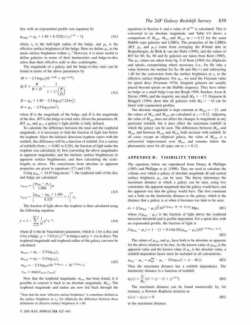
Figure 4. The observed distribution of the 2dFGRS data set mapped onto

the BBD, prior to volume and incompleteness correction. The contour lines

are set at 25, 100, 250, 500, 750, 1000, 1250, 1500 and 1750 galaxies per

bin. The minimum number of galaxies in a bin is 25.

Figure 5. The BBD of galaxies with m � 17:84 ^ 0:1 and mappe �

22:31 ^ 0:1: The contour lines are set at 0.01, 0.05, 0.10, 0.15 and 0.20

chance of the galaxy being in that bin.

The 2dF Galaxy Redshift Survey 831

q 2001 RAS, MNRAS 324, 825±841

5.3 Deriving V(M,m)

To convert the number of observed galaxies to number density per

Mpc3, a Malmquist correction is required, i.e., V(M,m). This

matrix reflects the volumes over which each M,m bin can be

observed. One option is to use visibility theory as prescribed by

Phillipps et al. (1990), and used to construct the constant volume

line in Fig. 3. While visibility is clearly a step in the right

direction, and preferable to applying a correction dependent on

magnitude only, its limitation is that it assumes idealized galaxy

profiles (i.e., it neglects the bulge component, seeing, star±galaxy

separation and other complications). Ideally, one would like to

extract the volume information from the data itself, and this is

possible by using a 1/Vmax type prescription, i.e., within each

O(M,m) bin, the maximum redshift at which a galaxy is seen is

determined and the volume derived from this redshift. The

advantages of using the data set rather than theory is that it

naturally incorporates all redshift-dependent selection biases.

However, the maximum redshift is susceptible to scattering from

higher visibility bins. An improved version is therefore to use the

90th percentile redshift, and to adjust O(M,m ) and I(M,m)

accordingly.

Although this requires rejecting 10 per cent of the data, it has

two distinct advantages. First, it ensures that the redshift

distribution in each bin has a sharp cut-off (as opposed to a

distribution which peters out). Secondly, it uses the entire data set

as opposed to the maximum redshift only. In the case where the

90th percentile is not exact, we take the galaxy nearest. Using

these redshifts, the volume can be calculated independently for

each bin, assuming an Einstein±de Sitter cosmology as follows:

V�M;m� � Vz90�M;m�zmin�M;m�; �19�

where

Vz90�M;m�zmin�M;m� �

�z90�M;m�

zmin�M;m�

scd2l

H0�1 1 z�3:5 dz; �20�

and s is the solid angle in steradians on the sky. dl is the

luminosity distance to the galaxy, and zmin is the minimum

distance over which a galaxy can be detected. zmin is calculated

from visibility theory (Phillipps et al. 1990; see also Appendix B),

adopting values for the maximum magnitude and maximum size

of mB � 14:00 mag and u � 200 arcsec respectively.

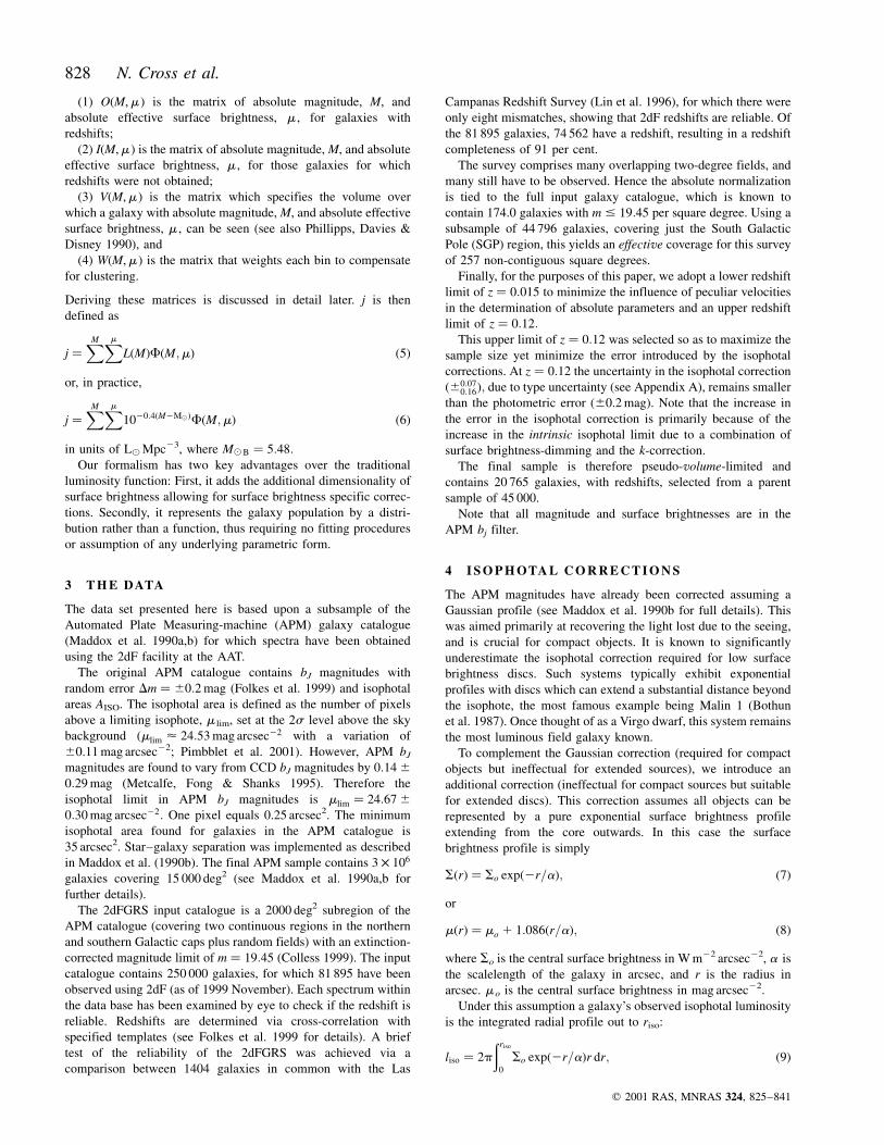
Fig. 8 shows the matrix 1V�M;m� : Note that squares containing

fewer than 25 galaxies are not shaded. This matrix is flat-

bottomed due to the cut-off at z � 0:12: Fig. 8 shows a strong

dependency upon magnitude (i.e., classical Malmquist bias as

expected) and also upon surface brightness. This surface bright-

ness dependency is particularly strong near the 104 Mpc3 volume

limit, as the data become sparse. Inside this volume limit the

contour lines generally mimic the curve of the visibility-derived

volume boundary. This suggests that visibility theory provides a

good description of the combined volume dependency. The sharp

cut-off along the high surface brightness edge may be real, but it

could also be a manifestation of the complex star±galaxy

Figure 6. The bivariate number distribution of those galaxies without

redshifts, i.e., I(M,m ). The contour lines are set at 10, 25, 50, 75, 100, 125

and 150 galaxies bin21.

Figure 7. The ratio of galaxies without redshifts to galaxies with redshifts.

The contour lines are set at 0.01, 0.05, 0.10, 0.15, 0.20, 0.25, 0.30, 0.35,

0.40, 0.45 and 0.50.

832 N. Cross et al.

q 2001 RAS, MNRAS 324, 825±841

separation algorithm (see Maddox et al. 1990a). Given that a

galaxy seen over a larger distance appears more compact, and that

local dwarfs have smaller scalelengths than giants (cf. Mateo

1998), this seems reasonable. We will investigate this further

through high-resolution imaging.

The main point to take away from Fig. 8 is that the visibility

surface of the 2dFGRS input catalogue is complex and dependent

on both M and me (though predominantly M). Any methodology

which ignores surface brightness information and implements a

volume-bias correction in luminosity only is implicitly assuming

uniform visibility in surface brightness. The 2dFGRS data clearly

show that this is not the case.

5.4 Clustering

Structure is seen on the largest measurable scales (e.g. de

Lapparent, Geller & Huchra 1986). To determine whether the

effects of clustering are significant, we constructed a radial

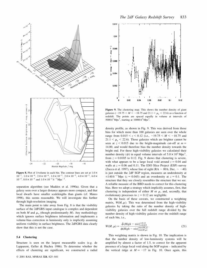
density profile, as shown in Fig. 9. This was derived from those

bins for which more than 100 galaxies are seen over the whole

range from 0:015 , z , 0:12 (i.e., 219:75 , M , 218:75 and

21:1 , me , 22:6�: Those galaxies which are brighter cannot be

seen at z , 0:015 due to the bright-magnitude cut-off at m �14:00; and would therefore bias the number density towards the

bright end. For these high-visibility galaxies we calculated their

number density (f) in equal volume intervals of 5:0 � 103 Mpc3;from z � 0:0185 to 0.12. Fig. 9 shows that clustering is severe,

with what appears to be a large local void around z � 0:04 and

walls at z � 0:06 and 0.11. The ESO Slice Project (ESP) survey

(Zucca et al. 1997), whose line of sight �RA , 00 h; Dec: , 240�is just outside the 2dF SGP region, measures an underdensity at

#140 h21 Mpc �z < 0:045� and an overdensity at z < 0:1: The

structure that they see closely resembles the structure that we see.

A reliable measure of the BBD needs to correct for this clustering

bias. Here we adopt a strategy which implicitly assumes, first, that

clustering is independent of either M or m, and, secondly, that

evolutionary processes to z � 0:12 are negligible.

On the basis of these caveats, we constructed a weighting

matrix, W(M,m). This was determined from the high-visibility

galaxies by taking the ratio of the number density of high-

visibility galaxies over the full redshift range divided by the

number density of high-visibility galaxies over the redshift range

of each bin, i.e.,

W�M;m� ��f �High 2 vis�z�0:12

z�0:015

f�High 2 vis�zmax�M;m�zmin�M;m�

: �21�

This weighting matrix is shown in Fig. 10. The implication is

that the number density of low-luminosity systems will be

amplified by almost a factor of 1.5, to correct for the apparent

presence of a large local void along the SGP region ± indicated by

the vertical ridge at M � 217 in Fig. 10. Once again, this

Figure 8. Plot of 1/volume in each bin. The contour lines are set at 1:0 �1027; 1:0 � 1026; 2:0 � 1026; 1:0 � 1025; 2:0 � 1025; 4:0 � 1025; 6:0 �1025; 8:0 � 1025 and 1:0 � 1024 h23 Mpc23:

Figure 9. The clustering map. This shows the number density of giant

galaxies �219:75 , M , 218:75 and 21:1 , me , 22:6� as a function of

redshift. The points are spaced equally in volume at intervals of

5000 h3 Mpc3, starting at 10000 h3 Mpc3.

The 2dF Galaxy Redshift Survey 833

q 2001 RAS, MNRAS 324, 825±841

implicitly assumes that the clustering of dwarf and giant systems

is correlated.

6 T H E 2 D F G R S B B D

Finally, we can combine the four matrices, O(M,m), I(M,m),

V(M,m ) and W(M,m) (see equation 4), to generate the 2dFGRS

bivariate brightness distribution, as shown in Fig. 11. This depicts

the underlying local galaxy number density distribution, inclusive

of surface brightness selection effects. Only those bins which are

based upon 25 or more galaxies are shown. Note that by summing

the BBD along the surface brightness axis, one recovers the

luminosity distribution of galaxies. By summing along the magni-

tude axis, one obtains the surface brightness distribution of

galaxies (see Section 8).

Fig. 12 shows the errors in the BBD. These were initially

determined via Monte Carlo simulations, assuming a Gaussian

error distribution of ^0.2 mag in the APM magnitudes. This

showed that the errors were proportional to�������������1=N�p

and, since

�������������1=N�pis much faster to calculate, this is the result that is used

throughout the calculations. These errors were then combined in

quadrature with the additional error in the volume estimate,

assuming Poisson statistics. The total error is given by

sf ��������������������������������������������������������

1

N tot�M;m�� �

11

Nz�M;m�� �s

: �22�

The errors become significant (. 20 per cent) when M . 216

and around the boundaries of the BBD shown in Fig. 11. The data

and associated errors are tabulated in Table C2. From Figs 11 and

12 we note the following.

6.1 A luminosity±surface brightness relation

The BBD shows evidence of a luminosity±surface brightness

Figure 10. The weighting map. The contours are at 0.8, 0.9, 1.0, 1.1, 1.2,

1.3, 1.4 and 1.5.

Figure 11. The 2dFGRS bivariate brightness distribution. The contour

lines are set at 1:0 � 1027; 1:0 � 1023; 2:5 � 1023; 5:0 � 1023; 7:5 � 1023;

1:0 � 1022; 1:25 � 1022; 1:5 � 1022; 1:75 � 1022; 2:0 � 1022; and 2:25 �1022 galaxies Mpc23 bin21: The thick lines represent the selection

boundaries calculated from visibility theory.

834 N. Cross et al.

q 2001 RAS, MNRAS 324, 825±841

relation similar to that seen in Virgo �MB / 1:6mo; Binggeli 1993)

in the Hubble Deep Field �MF450W / 1:5me; Driver 1999) and in

Sdm galaxies �MB / 2:02 ^ 0:16me; de Jong & Lacey 2000). A

formal fit to the 2dFGRS data yields MB / �2:4^1:50:5�me: While

confirming the general trend, this result appears significantly

steeper than the Virgo and HDF results. Both the Virgo and HDF

results are based on lower luminosity systems, and so this might

be indicative of a second-order dependency of the relation upon

luminosity. Alternatively, it may reflect slight differences in the

data/analysis, as neither the Virgo nor HDF data include isophotal

corrections, whereas the 2dFGRS data are more susceptible to

atmospheric seeing. The gradient is slightly steeper than the de

Jong & Lacey result, but is well within the errors.

The presence of a luminosity±surface brightness relation

highlights concerns over the completeness of galaxy surveys, as

surveys with bright isophotal limits will preferentially exclude

dwarf systems, leading to an underestimate of their space densities

and variations such as those seen in Fig. 1.

The confirmation of this luminosity±surface brightness relation

within such an extensive data set is an important step forward, and

any credible model of galaxy formation must now be required to

reproduce this relation.

6.2 A dearth of luminous, low surface brightness galaxies

Within each magnitude interval there appears to be a preferred

range in surface brightness over which galaxies may exist. While

the high surface brightness limit may be due, in part or whole, to

star±galaxy separation and/or fibre-positioning accuracy, the low

surface brightness limit appears to be real. It cannot be a selection

limit, as one requires a mechanism which hides luminous LSBGs

yet allows dwarf galaxies of similar surface brightness to be

detected within the same volume. The implications are that these

galaxy types (luminous LSBGs) are rare, with densities less than

1024 galaxies Mpc23. This result is important, as it directly

addresses the issues raised in the introduction, and implies that

existing surveys have not missed large populations of luminous

LSBGs. Perhaps more importantly, it confirms that the 2dFGRS is

complete for giant galaxies, and that the postulate that the

Universe might be dominated by luminous LSBGs (Disney 1976)

is ruled out.

One caveat, however, is that luminous LSBGs could be

masquerading as dwarfs. For example, consider the case of

Malin 1 (Bothun et al. 1987), which has a huge extended disc

(55 kpc scalelength) of very low surface brightness �mo � 26:5�:This system is actually readily detectable because of its high

surface brightness active core; however, within the 2dFGRS limits

it would have been misclassified as a dwarf system with M �217:9; me � 21:8: Hence Figs 11 and 12 rule out luminous disc

systems only. To determine whether objects such as Malin 1 are

hidden amongst the dwarf population will require either ultradeep

CCD imaging or cross-correlation with H i-surveys which would

exhibit very high H i mass-to-light ratios for such systems.

6.3 The rising dwarf population

The galaxy population shows a steady increase in number density

with decreasing luminosity. This continues to the survey limits at

M � 216; whereupon the volume limit and surface brightness

selection effects impinge upon our sample. The expectation is that

the distribution continues to rise, and hence the location of the

peak in the number density distribution remains unknown.

However, we do note that the increase seen within our selection

limits is insufficient for the dwarf population to dominate the

luminosity density, as shown in the next section.

Perhaps more surprising is the lack of substructure, indicating

either a continuity between the giant and dwarf populations or that

any substructure is erased by the random errors. The former case

is strongly indicative of a hierarchical merger scenario for galaxy

formation which one expects to lead towards a smooth number

density distribution between the dwarf and giant systems (White

& Rees 1978). This is contrary to the change in the luminosity

distribution of galaxies seen in cluster environments (e.g. Smith,

Driver & Phillipps 1997). In a later paper we intend to explore the

dependency of the BBD upon environment.

7 T H E VA L U E O F jB A N D VM

The luminosity density matrix j(M,m) is constructed from

LF(M,m) in units of L( Mpc23, and is shown as Fig. 13. The

distribution is strongly peaked close to the conventional Mpparameter derived in previous surveys (see Table C1). The peak

lies at M � 219:5 mag and me � 22:12 mag arcsec22: The final

value obtained is jB � �2:49 ^ 0:20� � 108 h100 L( Mpc23: The

sharp peak sits firmly in the centre of our observable region of

the 2dFGRS BBD, and drops rapidly off on all sides towards the

2dFGRS BBD boundaries. This implies that while the 2dFGRS

does not survey the entire parameter space of the known BBD, it

does effectively contain the full galaxy contribution to the local

luminosity density. Redoing the calculations using galaxies with

redshifts also results in jB � �2:49 ^ 0:20� � 108 h100 L( Mpc23:This demonstrates that there is no dependency of the results upon

the assumption made for the distribution of galaxies without

redshifts.

We note that j derived via a direct 1/Vmax estimate, without

any surface brightness or clustering corrections, (equation 1)

gives a value of j � 1:82 ^ 0:07 � 108 h100 L( Mpc23: Including

the isophotal magnitude correction only leads to a value of

Figure 12. The errors in the BBD. The contour lines are set at 1:0 � 1027;

1:0 � 1024; 5:0 � 1024; 1:0 � 1023; 1:5 � 1023; 2:0 � 1023; 2:5 � 1023;3:0 � 1023; 3:5 � 1023 and 4:0 � 1023 galaxies Mpc23 bin21:

The 2dF Galaxy Redshift Survey 835

q 2001 RAS, MNRAS 324, 825±841

j � 2:28 ^ 0:09 � 108 h100 L( Mpc23. Hence a more detailed

analysis leads to a 36.8 per cent increase in j, of which 25.3 per

cent is due to the isophotal correction, 10.4 per cent is due to the

Malmquist bias correction, and 1.1 per cent is due to the clustering

correction.

The final value agrees well with that obtained from the recent

ESO Slice Project (Zucca et al. 1997). The method that they used

corrects for clustering, but not surface brightness ± although their

photometry is based on aperture rather than isophotal magnitudes.

However, it is worth pointing out that j is sensitive to the exact

value of m lim. The quoted error in m lim is ^0.3 (for plate-to-plate

variations, see Metcalfe et al. 1995 and Pimblett et al. 2000).

Table C3 shows a summary of results when repeating the entire

analysis using the upper and lower error limits. It therefore seems

likely that a combination of surface brightness biases and large-

scale structure can indeed lead to the type of variations seen in

Table C1.

Finally, following the method of Carlberg, Yee & Ellingson

(1997), we can obtain a crude ball-park figure for the total local

mass density by adopting a universal mass-to-light ratio based on

that observed in clusters. While this method neglects biasing

(White, Tully & Davis 1988), it does provide a useful crude upper

limit to the mass density. From Carlberg et al. (1997) we find:

MDyn/LR � 289 ^ 50 h100 M(/L(: Assuming a mean colour of

�B 2 R� � 1:1 and a solar colour index of 1.17, this converts to:

MDyn/LB � 271 ^ 47 h100 M(/L(: Multiplying the luminosity

density by the mass-to-light ratio yields a value for the local

mass density of VM < 0:24: We note that this is consistent with

the current constraints from the combination of SN Ia results with

the recent Boomerang and Maxima-1 results (Balbi et al. 2000;

de Bernardis et al. 2000).

8 C O M PA R I S O N S W I T H OT H E R S U RV E Y S

As this work represents the first detailed measure of the field

BBD, there is no previous work with which to compare. However,

as mentioned earlier, it is trivial to convert the BBD into either a

luminosity distribution and/or a surface brightness distribution,

both of which have been determined by numerous groups. This is

achieved by summing across either luminosity or surface bright-

ness intervals. For those bins containing fewer than 25 galaxies for

which a volume- and clustering-bias correction were not obtained

we use the volume-bias correction from the nearest bin with 25 or

more galaxies. This will lead to a slight underestimate in the

number-densities; however, as the number density peak is well

defined, this effect is negligible.

8.1 The luminosity distribution

Fig. 14 shows a compendium of luminosity function measures (see

Table C1 and Fig. 1). Superimposed on the previous Schechter

function fits (dotted lines) are the results from the 2dFGRS. Three

results are shown, the luminosity distribution neglecting surface

brightness and clustering (short-dashed line), the luminosity

distribution inclusive of surface brightness corrections (long-

dashed line), and finally the luminosity distribution inclusive of

surface brightness and clustering corrections (solid line). The inset

shows the 2sx2 error eclipse for the last case, yielding Schechter

function parameters of Mp � 219:75 ^ 0:05; a � 21:09 ^ 0:03

Figure 13. Plot of the luminosity density distribution. The contour lines

are set at 100, 1:0 � 106; 5:0 � 106; 1:0 � 107; 2:0 � 107; 3:0 � 107; 4:0 �107; 5:0 � 107 and 6:0 � 107 L( Mpc23 bin21:

Figure 14. The solid line shows the final luminosity function, with all

corrections taken into account. The long-dashed line shows the LF with

surface brightness corrections only, and the short-dashed line shows the LF

ignoring surface brightness and clustering corrections. Also shown, as

dotted lines, are the LFs from Fig. 1. The shaded region denotes the limit

of reliability based on visibility theory.

836 N. Cross et al.

q 2001 RAS, MNRAS 324, 825±841

and fp � 0:0202 ^ 0:0002; in close agreement with the ESO

Slice Project (ESP) (see Table C1).

Comparing the 2dFGRS result with other surveys suggests that

the main effects of the surface brightness correction are to shift

Mp brightwards by the mean isophotal correction of 0.33 mag and

to increase the number density by a factor of 1.2. The clustering

correction has little effect at bright magnitudes, almost by

definition, but significantly amplifies the dwarf population. This

is a direct consequence of an apparent local void at z � 0:04 along

the full range of the 2dF SGP region.

We note that the combination of these two corrections closely

mimics the discrepancies between various Schechter function fits.

For example, the shallower SSRS2, APM and Durham/UKST

surveys are biased at all magnitudes by the apparent local void,

while the deeper ESP and Autofib surveys (which employ

clustering independent methods) probe beyond the void. Similarly,

because of the luminosity±surface brightness relation, those

surveys which probe to lower surface brightnesses will yield

higher dwarf-to-giant ratios.

The shaded region shows the point at which our data start to

become highly uncertain because of the small volume surveyed

�V , 10 000 Mpc3�: As this is the first statistically significant

investigation into the bivariate brightness distribution, we can

conclude that as yet no survey contains any direct census of the

space density of MB . 216:0 mag galaxies.

8.2 The surface brightness distribution

There have been a few surface brightness functions (SBFs)

published over the years. The first was the Freeman (1970) result,

which showed a Gaussian distribution with �m � 21:65 and sm �0:3: Since then, however, many galaxies have been found at

greater than 10s from the mean. The probability of a galaxy

occurring at 10s or greater is <1 � 10220: The total number of

galaxies in the Universe is in the range of 1011±1012, so the

Freeman SBF must be underestimating the LSBGs. The distribu-

tion seen by Freeman is almost certainly due to the relatively

bright isophotal detection threshold that the observations were

taken at, around 22±23 mag arcsec22. A more recent measure of

the SBF comes from O'Neil & Bothun (2000), who also show a

compendium of results from other groups. The O'Neil & Bothun

data, in contrast to the Freeman result, show a flat distribution

over the range 22 , mo , 25; albeit with substantial scatter.

Fig. 15 reproduces fig. 1. of O'Neil & Bothun, but now includes

the final 2dFGRS results. In order to compare our results directly

with the O'Neil & Bothun data, we assumed a mean bulge-to-total

ratio of 0.4 (see Kent 1985), resulting in a uniform offset of

0.55 mag arcsec22.

The 2dFGRS data are substantially broader than the Freeman

distribution, and appear to agree well with the compendium of

data summarized in O'Neil & Bothun (2000). From visibility

theory (see Fig. 3) our data are complete (i.e., the volume

observed is greater than 104 Mpc3 and therefore statistically

representative) in central surface brightness from 18:0 , mo , 23

for M , 216: Assuming that the luminosity±surface brightness

relation continues as reported in Driver (1999) and Driver & Cross

(2000), the expectation is that the surface brightness distribution

will steepen as galaxies with lower luminosities are included.

9 C O N C L U S I O N S

We have introduced the bivariate brightness distribution (BBD) as

a means by which the effect of surface brightness selection biases

in large galaxy catalogues can be investigated. By correcting for

the light below the isophote and including a surface brightness-

dependent Malmquist correction, we find that the measurement of

the luminosity density is increased by ,37 per cent over the

traditional 1/Vmax method of evaluation. The majority (25 per

cent) of this increase comes from the isophotal correction, with 10

per cent due to incorporating a surface brightness-dependent

Malmquist correction, and 1 per cent due to the clustering

correction.

We have shown that our isophotal correction is suitable for all

galaxy types, and that isophotal magnitudes without correction

severely underestimate the magnitudes for specific galaxy types.

We also note that the redshift incompleteness suggests that

predominantly low surface brightness galaxies are being missed;

however, we also show that these systems are predominantly low-

luminosity and hence contribute little to the overall luminosity

density. This is in part due to the high completeness of the

2dFGRS (,91 per cent).

We rule out the possibility of the 2dFGRS missing a significant

population of luminous giant galaxies down to me � 24:5 mag

arcsec22 (or mo � 23:5 mag arcsec22�; and note that the contribu-

tion at surface brightness limits below me � 23 mag arcsec22 is

small and declining. Dwarf galaxies greatly outnumber the giants,

and the peak in the number density occurs at the low-luminosity

selection boundary. The implication is that the most numerous

galaxy type lies at M . 216:0 mag: The galaxy population as a

whole follows a luminosity±surface brightness relation �M /�2:4^1:5

0:5�me� similar (but slightly steeper) to that seen in Virgo, in

the Hubble Deep Field and in SdM galaxies. This relation

provides an additional constraint which galaxy formation models

must satisfy.

We conclude that our measure of the galaxy contribution to the

luminosity density is robust and dominated by conventional giant

galaxies, with only a small (,10 per cent) contribution from

dwarf �M . 217:5 mag� and/or low surface brightness giants

�me . 23 mag arcsec22� within the selection boundaries �224 ,MB , 215:5 mag; 18:0 , me , 24:5 mag arcsec22�: However,

we cannot rule out the possibility of a contribution from an

Figure 15. The solid line shows the final surface brightness function, with

all the surface brightness and clustering corrections. The points are offset

towards the low surface brightness direction by 0.55 mag to crudely correct

for the bulge. Also shown are the O'Neil & Bothun (2000) data, as crosses

with error bars. The shaded region is where the visibility line shown in the

previous diagrams starts to cross the data, and so the data are no longer

completely reliable.

The 2dF Galaxy Redshift Survey 837

q 2001 RAS, MNRAS 324, 825±841

independent population outside of our optical selection

boundaries.

Our measurement of the luminosity density is j � 2:49 ^

0:20 � 108 h100 L( Mpc23; and using a typical cluster mass-to-

light ratio leads to an estimate of the matter density of order

VM , 0:24; in agreement with more robust measures.

Finally, we note that the bivariate brightness distribution offers

a means of studying the galaxy population and luminosity density

as a function of environment and epoch fully inclusive of surface

brightness selection biases. Future extensions to this work will

include the measurement of BBDs and `population peaks' for

individual spectral/morphological types, and as a function of

redshift and environment. This step forward has become possible

only because of the recent availability of large redshift survey data

bases such as that provided by the 2dFGRS.

AC K N OW L E D G M E N T S

The data shown here were obtained via the two-degree field

facility on the 3.9-m Anglo-Australian Observatory. We thank all

those involved in the smooth running and continued success of the

2dF and the AAO.

R E F E R E N C E S

Babul A., Ferguson H. C., 1996, ApJ, 458, 100

Babul A., Rees M., 1992, MNRAS, 255, 346

Balbi A. et al., 2000, ApJ, 545, L1

Beijersbergen M., de Blok W. J. G., van der Hulst J. M., 1999, A&A, 351,

903

Binggeli B., 1993, in Meylan G., Prugniel P., eds, ESO/OHP Workshop on

Dwarf Galaxies. ESO, Garching, p. 13

Binggeli B., Sandage A., Tammann G. A., 1988, ARA&A, 26, 509

Bothun G. D., Impey C. D., Malin D. F., Mould J. R., 1987, AJ, 94, 23

Boyce P. J., Phillipps S., 1995, A&A, 296, 26

Bristow P. D., Phillipps S., 1994, MNRAS, 267, 13

Carlberg R. G., Yee H. K. C., Ellingson E., Abraham R., Gravel P., Morris

S., Pritchet C. J., 1996, ApJ, 462, 32

Carlberg R. G., Yee H. K. C., Ellingson E., 1997, ApJ, 478, 462

Colless M., 1999, Phil. Trans. R. Soc., 357, 105

Dalcanton J. J., 1998, ApJ, 495, 251

Dalcanton J. J., Spergel D. N., Gunn J. E., Schmidt M., Schneider D. P.,

1997, AJ, 114, 635

de Bernardis P. et al., 2000, Nat, 404, 955

de Propris R., Pritchet C. J., Harris W. E., McClure R. D., 1995, ApJ, 450,

534

de Jong R., Lacey C., 2000, ApJ, 545, 781

de Lapparent V., Geller M. J., Huchra J. P., 1986, ApJ, 304, 585

de Vaucouleurs G., 1948, Ann. Astrophys., 11, 247

Disney M., 1976, Nat, 263, 573

Disney M., Phillipps S., 1983, MNRAS, 205, 1253

Driver S. P., 1999, ApJ, 526, L69

Driver S. P., Cross N. J. G., 2000, in Kraan-Korteweg R., Henning P.,

Andernach H., eds, ASP Conf. Ser. Vol. 218, Mapping the Hidden

Universe. Kluwer, Dordrecht, p. 309

Driver S. P., Phillips S., Davies J. I., Morgan I., Disney M. J., 1994,

MNRAS, 266, 155

Driver S. P., Windhorst R. A., Griffiths R. E., 1995, ApJ, 453, 48

Driver S. P., Couch W. J., Phillipps S., 1998, MNRAS, 301, 369

Efstathiou G., Ellis R., Peterson B., 1988, MNRAS, 232, 431

Ellis R. S., 1997, ARA&A, 35, 389

Ellis R. S., Colless M., Broadhurst T., Heyl J., Glazebrook K., 1996,

MNRAS, 280, 235

Felten J. E., 1985, Comments Astrophys., 11, 53

Ferguson H. C., Binggeli B., 1994, A&AR, 6, 67

FernaÂndez-Soto A., Lanzetta K., Yahil A., 1999, ApJ, 513, 34

Folkes S. et al., 1999, MNRAS, 308, 459

Freeman K., 1970, ApJ, 160, 811

Fukugita M., Hogan C. J., Peebles P. J. E., 1998, ApJ, 503, 518

Gaztanaga E., Dalton G. B., 2000, MNRAS, 312, 417

Impey C., Bothun G., 1997, ARA&A, 35, 267

Kent S. M., 1985, ApJS, 59, 115

Koo D. C., Kron R. G., 1992, ARA&A, 30, 613

Lilly S. J., Le FeÁvre O., Hammer F., Crampton D., 1996, ApJ, 460, 1

Lin H., Kirshner R., Shectman S., Landy S., Oemler A., Tucker D.,

Schechter P., 1996, ApJ, 464, 60

Loveday J., 1997, ApJ, 489, 29

Loveday J., 2000, MNRAS, 312, 557

Loveday J., Peterson B. A., Efstathiou G., Maddox S. J., 1992, ApJ, 390,

338

Madau P., Della Valle M., Panagia N., 1998, ApJ, 498, 106

Maddox S. J., Sutherland W. J., Efstathiou G., Loveday J., 1990a,

MNRAS, 243, 692

Maddox S. J., Efstathiou G., Sutherland W. J., 1990b, MNRAS, 246,

433

Margon B., 1999, Phil. Trans. R. Soc., 357, 105

Marzke R., Huchra J., Geller M., 1994, ApJ, 428, 43

Marzke R., Da Costa N., Pelligrini P., Willmer C., Geller M., 1998, ApJ,

503, 617

Mateo M. L., 1998, ARA&A, 36, 435

McGaugh S. S., 1996, MNRAS, 280, 337

Metcalfe N., Fong R., Shanks T., 1995, MNRAS, 274, 769

Minchin R. F., 1999, Publ. Astron. Soc. Aust., 16, 12

O'Neil K., Bothun G. D., 2000, ApJ, 529, 811

Persic M., Salucci P., 1992, MNRAS, 258, 14p

Petrosian V., 1998, ApJ, 507, 1

Phillipps S., Disney M., 1986, MNRAS, 221, 1039

Phillipps S., Driver S. P., 1995, MNRAS, 274, 832

Phillipps S., Davies J., Disney M., 1990, MNRAS, 242, 235

Phillipps S., Driver S. P., Couch W. J., Smith R. M., 1998, ApJ, 498, L119

Pimbblet K. A., Smail I., Edge A. C., Couch W. J., O'Hely E., Zabludoff

A. I., 2001, MNRAS, submitted

Ratcliffe A., Shanks T., Parker Q., Fong R., 1998, MNRAS, 293, 197

Schechter P., 1976, ApJ, 203, 297

Shanks T., 1990, in Bowyer S. C., Leinert C., eds, Proc. IAU Symp. 139,

Extragalactic Background Radiation. Kluwer, Dordrecht, p. 269

Smith R. M., Driver S. P., Phillipps S., 1997, MNRAS, 287, 415

Smoker J. V., Axon D. J., Davies R. D., 1999, A&A, 341, 725

Sodre L., Jr, Lahav O., 1993, MNRAS, 260, 285

Sprayberry D., Impey C., Irwin M., 1996, ApJ, 463, 535

Taylor K., Cannon R. D., Parker Q., 1998, in McLean B. J., Golembek

D. A., Haynes J. J. E., Payne H. E., eds, Proc. IAU Symp. 179, New

Horizons from Multi Wavelength Sky Surveys. Kluwer, Dordrecht,

p. 135

Trentham N., 1998, MNRAS, 294, 193

van den Bergh S., 1998, Galaxy Morphology and Classification.

Cambridge Univ. Press, Cambridge

Williams R. E. et al., 1996, AJ, 112, 1335

Willmer C. N. A., 1997, AJ, 114, 898

White S. D. M., Rees M. J., 1978, MNRAS, 183, 341

White S. D. M., Tully B., Davis M., 1988, ApJ, 333, L45

Zucca E. et al., 1997, A&A, 326, 477

A P P E N D I X A : T E S T I N G T H E I S O P H OTA L

C O R R E C T I O N S

It is possible to model several different types of galaxy, and to

compare the isophotal magnitude and the total magnitude as

calculated in Section 4 with the `true' magnitude. The models are

simple, assuming a face on circular galaxy, and composed of a

bulge with a de Vaucouleurs r14 law (de Vaucouleurs 1948) and a

838 N. Cross et al.

q 2001 RAS, MNRAS 324, 825±841

disc with an exponential profile (see equation 8):

mbulge � me 1 1:40 1 8:325��r=re�1=4 2 1�; �A1�where re is the half-light radius of the bulge, and me is the

effective surface brightness of the bulge. Here we define me as the

mean surface brightness within re.3 However, it is more useful to

define galaxies in terms of their luminosities and bulge-to-disc

ratios than their effective radii or disc scalelengths.

The magnitude of a galaxy and the bulge-to-disc ratio can be

found in terms of the above parameters by

M � 22:5 log10�1020:4B 1 1020:4D�

B=T � B

B 1 D� 1

1 1 1=B

D

� �B � me 1 1:40 2 2:5 log10�7:22pr2

e�D � mo 2 2:5 log10�pa2�;

�A2�

where B is the magnitude of the bulge, and D is the magnitude

of the disc. B/T is the bulge-to-total ratio. Given the parameters M,

B/T, me and mo, a galaxy's light profile is fully defined.

To calculate the difference between the total and the isophotal

magnitude, it is necessary to find the fraction of light lost below

the isophote. Since the intrinsic detection isophote varies with the

redshift, this difference will be a function of redshift. For a variety

of redshifts from z � 0:001 to 0.201, the fraction of light under the

isophote was calculated, by first converting the above magnitudes

to apparent magnitudes, and the intrinsic surface brightnesses to

apparent surface brightnesses, and then calculating the scale-

lengths as above. The conversions from absolute to apparent

properties are given in equations (17) and (18).

Using mlim � 24:67 mag arcsec22; the isophotal radii of the disc

and bulge are calculated:

riso;d � mlim 2 mo

1:086

� �a

riso;b � mlim 2 �me 1 1:40�8:325

1 1

� �4

re:

�A3�

The fraction of light above the isophote is then calculated using

the following equation:

f � 1 2X2b21

n�0

1

n!gn e2g; �A4�

where b is the de Vaucouleurs parameter, which is 1 for a disc and

4 for a bulge. g � 7:67 r/re� �1=4 in bulges and g � r/a in discs. The

isophotal magnitude and isophotal radius of the galaxy can now be

calculated:

miso;b � mb 2 2:5 log10 f b

miso;d � md 2 2:5 log10 f d

miso � 22:5 log10�1020:4miso;b 1 1020:4miso;d �riso � max�riso;b; riso;d�

: �A5�

Now that the isophotal magnitude, miso, has been found, it is

possible to convert it back to an absolute magnitude, Miso. The

isophotal magnitude and radius are now fed back through the

equations in Section 4, and a value of mcorr is calculated. This is

converted to an absolute magnitude, and Table C4 shows a

comparison of Mtrue, Miso and Mcorr at z � 0:12 for the main

Hubble type galaxies and LSBGs. The properties of the LSBGs

(B/T, me and mo) come from averaging the B-band data in

Beijersbergen, de Blok & van der Hulst (1999), and the values of

B/T for S0, Sa, Sb and Sc galaxies are taken from Kent (1985).

The me values are taken from fig. 5 of Kent (1985) for ellipticals

and spirals, extrapolating where necessary (i.e., for Sb, take a

value between the median for Sa±Sb and Sbc1) and subtracting

1.40 for the conversion from the surface brightness at re to the

effective surface brightness. For mo, we used the Freeman value

for spiral discs (Freeman 1970). Irregular galaxies are usually

placed beyond spirals on the Hubble sequence. They have either

no bulge or a small bulge (van den Bergh 1998; Smoker, Axon &

Davies 1999), and the majority are small MB . 217: Ferguson &

Binggeli (1994) show that all galaxies with MB . 216 can be

fitted with exponential profiles.

The absolute magnitude is kept constant at Mtrue � 221; and

the values of Miso and Mcorr are calculated at z � 0:12: Adjusting

the value of Mtrue does not affect the changes in magnitude at any

particular redshift, but it does effect the maximum redshift at

which the galaxy can be seen. The differences between Miso and

Mtrue and between Mcorr and Mtrue both increase with redshift. In

all cases except an elliptical galaxy, the value of Mcorr is a

substantial improvement over Miso, and remains below the

photometric error for all types out to z � 0:12:

A P P E N D I X B : V I S I B I L I T Y T H E O RY

The equations below are reproduced from Disney & Phillipps

(1983) and Phillipps et al. (1990). They are used to calculate the

volume over which a galaxy of absolute magnitude M and central

surface brightness mo can be seen. The theory determines the

maximum distance at which a galaxy can be seen, using two

constraints: the apparent magnitude that the galaxy would have, and

the apparent size that the galaxy would have. The first constraint

sets a limit on the luminosity distance to the galaxy, which is the

distance that a galaxy is at when it becomes too faint to be seen:

d1 � �f �mlim 2 mo��1210{0:2�mlim2M2252K�z��} Mpc; �B1�

where f �mlim 2 mo� is the fraction of light above the isophotal

detection threshold and is profile-dependent. For a spiral disc with

an exponential profile, the fraction of light is

f �mlim 2 mo� � 1 2 �1 1 0:4 ln�10��mlim 2 mo��10�20:4�mlim2mo��:�B2�

The values of m lim and mo have both to be absolute or apparent

for the above relation to be true. As the known value of m lim is the

apparent value and the known value of mo is the absolute value, a

redshift-dependent factor must be included in all calculations:

mlim 2 mo ! mapplim 2 mo 2 10 log10�1 1 z�2 K�z�: �B3�

Thus the maximum distance has a redshift dependence. The

luminosity distance is a function of redshift:

dL�z� � 2c

H0

��1 1 z�2 �1 1 z�10:5�: �B4�The maximum distance can be found numerically by, for

instance, a Newton±Raphson iteration as

d1�z�2 dL�z� � 0 �B5�at the maximum distance.

3 Note that the term `effective surface brightness' is sometimes defined as

the surface brightness at re; for ellipticals the difference between these

definitions of effective surface brightness is 1.40.

The 2dF Galaxy Redshift Survey 839

q 2001 RAS, MNRAS 324, 825±841

The second constraint, the size limit, is found by a similar

methodology. The formulation of the size limit is

d2 � Cg�mlim 2 mo�10�0:2�mo2M��=ulim Mpc; �B6�where C is a profile-dependent constant. g�mlim 2 mo� is the

isophotal radius in scalelengths. u lim is the minimum apparent

diameter. For a spiral disc with an exponential profile

C � 2������2pp 1025 �B7�

g�mlim 2 mo� � 0:4 ln�10��mapplim 2 mo 2 10 log10�1 1 z�2 K�z��:

�B8�In this case d2 is an angular-diameter distance, not a luminosity

distance:

dA�z� � 2c

H0

��1 1 z�21 2 �1 1 z�21:5� �B9�

d2�z�2 dA�z� � 0: �B10�Once the redshifts z1 and z2, which are the solutions of

equations (B5) and (B10), have been found, the maximum redshift

at which the galaxy can be seen is the minimum of z1 and z2:

zmax � min�z1; z2�: �B11�For the 2dFGRS, the parameters above are mlim �

24:67 mag arcsec22; mlim � 19:45 mag; and ulim � 7:2 arcsec:zmax # 0:12 is another limit imposed on this survey.

There are also limits on the minimum redshift. These are

also caused by selection effects in the survey. One limit comes

from the maximum apparent brightness of galaxies in the

sample, which is m � 14:00: The minimum redshift, z3, is

calculated just as z1. There is a also a maximum radius for

galaxies, which is umax � 200 arcsec: This comes from the sky-

subtraction process. This leads to z4, calculated in the same

way as z2:

zmin � max�z3; z4�; �B12�where zmin $ 0:015: This limit is to prevent peculiar velocities

dominating over the Hubble flow velocity. Also,

V�M;mo� ��zmax�M;mo�

zmin�M;mo�

scd2L

H0�1 1 z�3:5 dz; �B13�

where s is the area on the sky in steradians, c is the speed of light,

and H0 is Hubble's constant. The visibility V(M,mo) represents the

volume over which a spiral disc galaxy of absolute magnitude M

and central surface brightness mo can be observed. The central

surface brightness can be converted to effective surface brightness

using the following formula:

me � mo 1 1:124: �B14�

A P P E N D I X C : TA B L E S

Table C1. A comparison of the local luminosity density from recent magnitude-limited redshift surveys.

Survey Reference M* f* a jB/108 h100 L( Mpc23

SSRS2 Marzke et al. (1998) 219.43 1.28� 1022 21.12 1.28Durham/UKST Ratcliffe et al. (1998) 219.68 1.7� 1022 21.04 2.02ESP Zucca et al. (1997) 219.61 2.0� 1022 21.22 2.58LCRS* Lin et al. (1996) 219.19 1.9� 1022 20.70 1.26EEP Efstathiou et al. (1988) 219.68 1.56� 1022 21.07 1.89Stromlo/APM Loveday et al. (1992) 219.50 1.40� 1022 20.97 1.35Autofib Ellis et al. (1996) 219.20 2.6� 1022 21.09 2.05CfA*2 Marzke et al. (1994) 219.15 2.4� 1022 21.00 1.71

* The LCRS used a Gunn r filter. The value of M* has been converted to MB using kbj 2 Rlo � 1:1 for theJohnson B band (Lin et al. 1996). *2 The CfA used Zwicky magnitudes. The value of M* has beenconverted to MB using kbj 2 MZ lo � 20:35 for the Johnson B band, and f* has been reduced by 60 percent (Gaztanaga & Dalton 2000).

840 N. Cross et al.

q 2001 RAS, MNRAS 324, 825±841

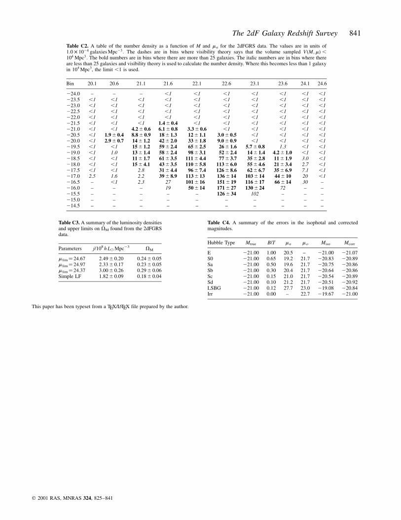
This paper has been typeset from a TEX/LATEX file prepared by the author.

Table C2. A table of the number density as a function of M and me for the 2dFGRS data. The values are in units of1:0 � 1024 galaxies Mpc23: The dashes are in bins where visibility theory says that the volume sampled V�M;m� ,104 Mpc3: The bold numbers are in bins where there are more than 25 galaxies. The italic numbers are in bins where thereare less than 25 galaxies and visibility theory is used to calculate the number density. Where this becomes less than 1 galaxyin 104 Mpc3, the limit ,1 is used.

Bin 20.1 20.6 21.1 21.6 22.1 22.6 23.1 23.6 24.1 24.6

224.0 ± ± ± ,1 ,1 ,1 ,1 ,1 ,1 ,1223.5 ,1 ,1 ,1 ,1 ,1 ,1 ,1 ,1 ,1 ,1223.0 ,1 ,1 ,1 ,1 ,1 ,1 ,1 ,1 ,1 ,1222.5 ,1 ,1 ,1 ,1 ,1 ,1 ,1 ,1 ,1 ,1222.0 ,1 ,1 ,1 ,1 ,1 ,1 ,1 ,1 ,1 ,1221.5 ,1 ,1 ,1 1.4^ 0.4 ,1 ,1 ,1 ,1 ,1 ,1221.0 ,1 ,1 4.2^ 0.6 6.1^ 0.8 3.3^ 0.6 ,1 ,1 ,1 ,1 ,1220.5 ,1 1.9^ 0.4 8.8^ 0.9 18^ 1.3 12^ 1.1 3.0^ 0.5 ,1 ,1 ,1 ,1220.0 ,1 2.9^ 0.7 14^ 1.2 42^ 2.0 33^ 1.8 9.0^ 0.9 ,1 ,1 ,1 ,1219.5 ,1 ,1 15^ 1.2 59^ 2.4 65^ 2.5 26^ 1.6 5.7^ 0.8 1.3 ,1 ,1219.0 ,1 1.0 13^ 1.4 58^ 2.4 98^ 3.1 52^ 2.4 14^ 1.4 4.2^ 1.0 ,1 ,1218.5 ,1 ,1 11^ 1.7 61^ 3.5 111^ 4.4 77^ 3.7 35^ 2.8 11^ 1.9 3.0 ,1218.0 ,1 ,1 15^ 4.1 43^ 3.5 110^ 5.8 113^ 6.0 55^ 4.6 21^ 3.4 2.7 ,1217.5 ,1 ,1 2.8 31^ 4.4 96^ 7.4 126^ 8.6 62^ 6.7 35^ 6.9 7.1 ,1217.0 2.5 1.6 2.2 39^ 8.9 113^ 13 136^ 14 103^ 14 44^ 10 20 ,1216.5 ± ,1 2.3 27 101^ 16 151^ 19 116^ 17 66^ 14 30 ±216.0 ± ± ± 19 50^ 14 171^ 27 130^ 24 72 ± ±215.5 ± ± ± ± ± 126^ 34 102 ± ± ±215.0 ± ± ± ± ± ± ± ± ± ±214.5 ± ± ± ± ± ± ± ± ± ±

Table C3. A summary of the luminosity densitiesand upper limits on VM found from the 2dFGRSdata.

Parameters j/108 h L( Mpc23 VM

m lim� 24.67 2.49^ 0.20 0.24^ 0.05m lim� 24.97 2.33^ 0.17 0.23^ 0.05m lim� 24.37 3.00^ 0.26 0.29^ 0.06Simple LF 1.82^ 0.09 0.18^ 0.04

Table C4. A summary of the errors in the isophotal and correctedmagnitudes.

Hubble Type Mtrue B/T me mo Miso Mcorr

E 221.00 1.00 20.5 ± 221.00 221.07S0 221.00 0.65 19.2 21.7 220.83 220.89Sa 221.00 0.50 19.6 21.7 220.75 220.86Sb 221.00 0.30 20.4 21.7 220.64 220.86Sc 221.00 0.15 21.0 21.7 220.54 220.89Sd 221.00 0.10 21.2 21.7 220.51 220.92LSBG 221.00 0.12 27.7 23.0 219.08 220.84Irr 221.00 0.00 ± 22.7 219.67 221.00

The 2dF Galaxy Redshift Survey 841

q 2001 RAS, MNRAS 324, 825±841