The 2-Coordinate Descent Method for Solving Double-Sided ...
28
J Optim Theory Appl (2014) 162:892–919 DOI 10.1007/s10957-013-0491-5 The 2-Coordinate Descent Method for Solving Double-Sided Simplex Constrained Minimization Problems Amir Beck Received: 11 November 2012 / Accepted: 19 November 2013 / Published online: 3 December 2013 © Springer Science+Business Media New York 2013 Abstract This paper considers the problem of minimizing a continuously differen- tiable function with a Lipschitz continuous gradient subject to a single linear equal- ity constraint and additional bound constraints on the decision variables. We intro- duce and analyze several variants of a 2-coordinate descent method: a block descent method that performs an optimization step with respect to only two variables at each iteration. Based on two new optimality measures, we establish convergence to station- arity points for general nonconvex objective functions. In the convex case, when all the variables are lower bounded but not upper bounded, we show that the sequence of function values converges at a sublinear rate. Several illustrative numerical examples demonstrate the effectiveness of the method. Keywords Nonconvex optimization · Simplex-type constraints · Block descent method · Rate of convergence 1 Introduction Block descent algorithms are methods in which an optimization problem is solved by performing at each iteration a minimization step with respect to a small number of de- cision variables while keeping all other variables fixed. This kind of approach is also referred to in the literature as a “decomposition” approach. One of the first variable decomposition methods for solving general minimization problems was the so-called alternating minimization method [1, 2], which is based on successive global mini- mization with respect to each component vector in a cyclic order. This fundamental Communicated by Gianni Di Pillo. A. Beck (B ) Faculty of Industrial Engineering and Management, Technion—Israel Institute of Technology, Haifa 32000, Israel e-mail: [email protected]
Transcript of The 2-Coordinate Descent Method for Solving Double-Sided ...
J Optim Theory Appl (2014) 162:892–919DOI 10.1007/s10957-013-0491-5
The 2-Coordinate Descent Methodfor Solving Double-Sided SimplexConstrained Minimization Problems
Amir Beck
Received: 11 November 2012 / Accepted: 19 November 2013 / Published online: 3 December 2013© Springer Science+Business Media New York 2013
Abstract This paper considers the problem of minimizing a continuously differen-tiable function with a Lipschitz continuous gradient subject to a single linear equal-ity constraint and additional bound constraints on the decision variables. We intro-duce and analyze several variants of a 2-coordinate descent method: a block descentmethod that performs an optimization step with respect to only two variables at eachiteration. Based on two new optimality measures, we establish convergence to station-arity points for general nonconvex objective functions. In the convex case, when allthe variables are lower bounded but not upper bounded, we show that the sequence offunction values converges at a sublinear rate. Several illustrative numerical examplesdemonstrate the effectiveness of the method.
Keywords Nonconvex optimization · Simplex-type constraints · Block descentmethod · Rate of convergence
1 Introduction
Block descent algorithms are methods in which an optimization problem is solved byperforming at each iteration a minimization step with respect to a small number of de-cision variables while keeping all other variables fixed. This kind of approach is alsoreferred to in the literature as a “decomposition” approach. One of the first variabledecomposition methods for solving general minimization problems was the so-calledalternating minimization method [1, 2], which is based on successive global mini-mization with respect to each component vector in a cyclic order. This fundamental
Communicated by Gianni Di Pillo.
A. Beck (B)Faculty of Industrial Engineering and Management, Technion—Israel Institute of Technology,Haifa 32000, Israele-mail: [email protected]
J Optim Theory Appl (2014) 162:892–919 893
method appears in the literature under various names such as the block-nonlinearGauss-Seidel method or the block coordinate descent method (see, e.g., [3–11]). Theconvergence of the method was extensively studied in the aforementioned papers un-der various assumptions such as the existence of error bounds, strict/strong convexitywith respect to each block, or uniqueness of minimizers with respect to each block.
Other block descent methods, that do not require a full minimization step at eachiteration, are for example those who employ at each iteration a gradient projectionstep with respect to the chosen indices subset. These methods have a clear advantageover alternating minimization when exact minimization with respect to each of thecomponent blocks is not an easy task. In [12] Luo and Tseng studied the convergenceof such a block gradient descent method for specially structured convex problemswith strict convexity assumptions on some of the elements of the objective functionand with box constraints. More general descent directions were studied by Polak etal. in [13] and also by Sargent and Sebastian in [14]. Convergence to stationary pointswas established by Tseng and Yun [15] for the nonconvex case when the objectivefunction has separable nonsmooth components. There seem to be only a few resultsin the literature on the rate of convergence of the sequence of function values in theabsence of assumptions such as strong/strict convexity or the existence of an errorbound. One such result was obtained by Nesterov in [16], where he showed that ifthe blocks are randomly chosen, then a sublinear rate of convergence of the expectedsequence of function values can be derived. Later on in [17] it was shown that if theblock selection is done in a cyclic manner, a sublinear rate of convergence can bederived.
All the mentioned works assume that the problem is either unconstrained or con-sists of block-wise constraints. When additional linear constraints are imposed, theblock-wise structure collapses and a different line of analysis is required. The firstalgorithms for this class of problems were proposed for solving the dual of the sup-port vector machine (SVM) optimization problem [18]. Hence, they are defined forthe subclass of quadratic convex functions. In the quadratic case, part of the strengthof 2-coordinate descent methods is in the fact that exact minimization can be ana-lytically performed. Platt’s sequential minimal optimization (SMO) algorithm [19]was the first 2-coordinate descent method with exact minimization. The simplicityand practical efficiency of the method motivated a vast amount of theoretical andpractical research on the convergence of the method, as well as modifications andimprovements. Later, Keerthi et al. in [20, 21] proposed a modified SMO methodbased on a kind of “most descent” choice of the coordinates. The so-called SVMlight
method proposed in [22] uses the same index selection strategy; in fact, it is more gen-eral in the sense that the method performs the optimization with respect to q chosenvariables—q being an even positive integer. Convergence was proved in [23, 24] forthe quadratic convex problem. A decomposition method based on the same selectionrule for a block of variables was defined for more general smooth functions in [25],also allowing inexact minimization of the subproblems and odd values of q . Latermethods for the more general (and even nonconvex) smooth problem were proposed;these methods are based on different selection rules and use either first order infor-mation [25–27], and might not require any ordering (e.g., cyclic selection rule) [28],or second order rules [29, 30]. All these methods are proved to have asymptotic con-vergence under quite mild assumptions. In [31–33], methods based on the projected
894 J Optim Theory Appl (2014) 162:892–919
gradient (PG) direction have been proposed. Later, Tseng and Yun [34] studied theconvergence of a coordinate (projected) gradient descent method for solving the gen-eral model of linearly constrained smooth minimization problems, which includes thedual SVM problem as a special case. A possible distributed version of a block-typemethod has also been proposed in [35].
In this paper, we consider the problem of minimizing a continuously differentiablefunction subject to a single linear constraint with additional bound constraints on thedecision variables; a precise definition of the problem is presented in Sect. 2. We con-sider several variations of a block descent method, which we call the 2-coordinatedescent method, that involves at each iteration the (possible approximated) solutionof the optimization problem with respect to only two variables while keeping allother variables fixed; the two-dimensional minimization subproblems can also bereduced into one-dimensional optimization problems. After discussing several nec-essary mathematical preliminaries in Sect. 3, that lay the ground for the basic ter-minology in the paper, we present and analyze in Sect. 4 two “optimality measures”which will be the basis for the construction and analysis of the 2-coordinate descentmethods devised in Sect. 5. The different variants of the method are dictated by theindex selection strategy (i.e., which indices are chosen at iteration) and by the step-size selection strategy (full or partial). We show the convergence of the correspondingoptimality measures in the nonconvex case. In the convex case, when all the variablesare lower bounded but not upper bounded (as in the case of the unit simplex), weshow in Sect. 6 a sublinear rate of convergence of the sequence of function values.The paper ends in Sect. 7, where several numerical experiments demonstrate the po-tential of the method.
2 Problem Formulation and Setting
We begin by describing some of the notation that will be used throughout the paper.For a positive integer i, the vector ei denotes the i-th canonical basis vector, that is, itconsists of zeros except for the i-th entry which is equal to one. For a differentiablefunction f , the gradient is denoted by ∇f and we use the notation ∇if for the i-thpartial derivative. For a closed and convex set X, the orthogonal projection onto theset X is denoted by PX(·) and defined by PX(y) := argmin{‖x − y‖ : x ∈ X}. Vectorsare denoted by boldface lowercase letters, and matrices by boldface uppercase letters.
The main problem we consider in this paper is
(P) min{f (x) : x ∈ �K,l,u
n
},
where the feasible set is given by:
�K,l,un :=
{
x ∈ Rn :
n∑
i=1
xi = K, li ≤ xi ≤ ui
}
.
Here K ∈R and for each i, ui ∈R∪ {∞} and li ∈R∪ {−∞}. We will call such a seta double-sided simplex set. We assume that li < ui for all i and, in order to ensure

J Optim Theory Appl (2014) 162:892–919 895
feasibility, we also assume that∑n
i=1 li ≤ K ≤ ∑ni=1 ui . Note that we do allow some
or all of the upper and lower bounds to be infinite, and we will use the usual arithmeticof infinite numbers (e.g., ∞ + a = ∞ for all a ∈R).
We will also be interested in the special case when there are no finite upper bounds,that is, ui = ∞ for all i = 1,2, . . . , n. In this case, the set will be called a one-sidedsimplex set and is given by (the superscript u can be omitted in this case):
�K,ln :=
{
x ∈Rn :
n∑
i=1
xi = K,xi ≥ li , i = 1, . . . , n
}
.
When K = 1 and l = 0, the one-sided simplex �1,0n is called the unit simplex:
�n :={
x ∈ Rn :
n∑
i=1
xi = 1, x1, . . . , xn ≥ 0
}
.
Despite the fact that a one-sided simplex set is also a two-sided simplex set, we willsee that in some parts of the analysis it is worthwhile to take special care for thissubclass of problems, since the results for the one-sided setting are sometimes simplerand stronger than those that can be obtained in the more general two-sided setting.
The following set of assumptions is made throughout the paper.
Assumption 1
• The objective function f : �K,l,un → R is continuously differentiable with Lipschitz
continuous gradient with constant L over �K,l,un , that is,
‖∇f (x) − ∇f (y)‖ ≤ L‖x − y‖ for all x,y ∈ �K,l,un .
• Problem (P) is solvable, that is, it has a nonempty optimal solution set denoted byX∗. The optimal value will be denoted by f ∗.
There are numerous minimization problems over two-sided simplex domains.Among them is the dual problem associated with the problem of training an SVM,which is a convex quadratic programming problem [18]. Another problem of type(P) is the standard quadratic programming problem (StQP), which requires the mini-mization of a quadratic function over the unit simplex, which arises, for example, inthe Markowitz portfolio optimization problem [36] and as the continuous formula-tion of combinatorial problems [37]. Another interesting problem is the dual of theChebyshev center problem [38]. Some of these examples will be discussed in detailin Sect. 7.
2.1 General Linear Constraint
A seemingly more general problem than (P) is
min
{
g(y) :n∑
i=1
aiyi = K,mi ≤ yi ≤ Mi, i = 1,2, . . . , n
}
, (1)
896 J Optim Theory Appl (2014) 162:892–919
where ai �= 0 for all i = 1,2, . . . , n and mi,Mi, i = 1,2, . . . , n are such that thefeasible set is nonempty. However, problem (1) is not actually more general sincewe can easily recast it in the form of model (P) by making the change of variablesxi = aiyi, i = 1,2, . . . , n, resulting in the problem:
min
{
g
(x1
a1, . . . ,
xn
an
):
n∑
i=1
xi = K,mi ≤ xi ≤ Mi, i = 1,2, . . . , n
}
, (2)
where
mi ={ mi
aiai > 0
Mi
aiai < 0,
Mi ={
Mi
aiai > 0
mi
aiai < 0.
Problem (2) fits model (P) with li = mi, ui = Mi and f (x) := g(x1a1
, . . . , xn
an). For
simplicity of presentation we will analyze the model (P); however, as will be shownin the sequel, the results and algorithms can be described also for the more generalmodel (1) by using the simple transformation just described.
3 Mathematical Preliminaries
Our main objective is to construct a block descent method that performs a minimiza-tion step with respect to two variables at each iteration. The coupling constraint (thatis, the constant sum constraint) prevents the development of an algorithm that per-forms a minimization with respect to only one variable at each iteration. We willtherefore be interested in the restriction of the objective function f on feasible direc-tions consisting of only two nonzero components.
Since we are interested in the feasible directions with two nonzero components,we will define for any z ∈ �
K,l,un and any two different indices the following function:
φi,j,z(t) := f(z + t (ei − ej )
), t ∈ Ii,j,z,
where the interval Ii,j,z comprises the feasible steps, that is,
Ii,j,z := {t : z + t (ei − ej ) ∈ �K,l,u
n
}.
A simple computation shows that Ii,j,z can be written explicitly as
Ii,j,z = [max{li − zi, zj − uj },min{ui − zi, zj − lj }
].
The derivative of φi,j,z(t) is given by
φ′i,j,z(t) = ∇if
(z + t (ei − ej )
) − ∇j f(z + t (ei − ej )
). (3)
The Lipschitz continuity of ∇f implies the Lipschitz continuity of φ′i,j,z(t) over
Ii,j,z, and for any i, j we will denote by Li,j the constant for which:
∣∣φ′i,j,z(t) − φ′
i,j,z(s)∣∣ ≤ Li,j |t − s|, for all z ∈ �K,l,u
n , t, s ∈ Ii,j,z.

J Optim Theory Appl (2014) 162:892–919 897
The constants Li,j will be called the local Lipschitz constants, and they satisfy thefollowing bound:
Li,j ≤ 2L.
Indeed, note that by (3) we have that
∣∣φ′i,j,z(t) − φ′
i,j,z(s)∣∣ = ∣∣(ei − ej )∇f (z + t (ei − ej ) − (ei − ej )∇f (z + s(ei − ej )
∣∣
≤ ‖ei − ej‖∥∥∇f (z + t (ei − ej ) − ∇f (z + s(ei − ej )
∥∥
≤ ‖ei − ej‖ · L|t − s| · ‖ei − ej‖ = L‖ei − ej‖2 · |t − s|= 2L|t − s|.
Example 3.1 Suppose that the objective function is a quadratic function of the form
f (x) = 1
2xT Qx + bT x,
where b ∈Rn and Q = QT ∈R
n×n. Then denoting d = ei −ej , after some rearrange-ment of terms, we have that
φi,j,z(t) = f (z + td)
= 1
2
(dT Qd
)t2 + dT (Qz + b)t + 1
2zT Qz + bT z.
Therefore,
φ′i,j,z(t) = (
dT Qd)t + dT (Qz + b) = (Qii + Qjj − 2Qij )t + dT (Qz + b),
and thus
Li,j = Qii + Qjj − 2Qij . (4)
4 Optimality Conditions and Measures
4.1 Conditions for Stationarity
We recall some well-known elementary concepts on optimality conditions for linearlyconstrained differentiable problems; for more details see, e.g., [6]. A vector x∗ ∈�
K,l,un is called stationary if
⟨∇f(x∗),x − x∗⟩ ≥ 0 for all x ∈ �K,l,u
n .
If x∗ is an optimal solution of (P), then it is also stationary. Therefore, stationarity isa necessary condition for optimality. When f is in addition convex, then stationarityis a necessary and sufficient condition for optimality. Since the problem at hand is

898 J Optim Theory Appl (2014) 162:892–919
linearly constrained, it follows that x∗ is a stationary point if and only if the Karush-Kuhn-Tucker (KKT) conditions are satisfied, meaning that x∗ ∈ �
K,l,un is a stationary
point of (P) if and only if there exists λ ∈R for which
∇if(x∗) =
⎧⎨
⎩
= λ li < x∗i < ui,
≤ λ x∗i = ui,
≥ λ x∗i = li ,
i = 1,2, . . . , n.
The above characterization of optimality is stated in terms of a dual variable. It is alsopossible to rewrite the exact same condition solely in terms of the primal decisionvariables vector: x∗ is a stationary point of (P) if and only if
minj :x∗
j <uj
∇j f(x∗) ≥ max
i:x∗i >li
∇if(x∗). (5)
Remark 4.1 When the feasible set is the unit simplex (K = 1, l = 0, ui = ∞, i =1, . . . , n), condition (5) takes the form
minj=1,...,n
∇j f(x∗) ≥ max
i:x∗i >0
∇if(x∗), (6)
and when there are no finite bounds, that is, when li = −∞ and ui = ∞ for alli = 1, . . . , n, condition (5) takes the form
minj=1,...,n
∇j f(x∗) ≥ max
i=1,...,n∇if
(x∗), (7)
which of course just means that all the partial derivatives ∇if (x∗) have the samevalue.
4.2 The Double-Sided Optimality Measure
The optimality condition (5) naturally calls for the following “optimality measure”(see also [39]):
R(x) = max{
maxi:x∗
i >li
∇if(x∗) − min
j :x∗j <uj
∇j f(x∗),0
}.
The above quantity is an optimality measure in the sense that it is positive for allnonstationary feasible points and zero for stationary points. However, it is actuallya rather poor optimality measure because it is not even continuous, as the followingexample illustrates.
Example 4.1 Consider the problem
min{(x1 + 2x2)
2 : x1 + x2 = 1, x1, x2 ≥ 0}. (8)
The optimal solution of problem (8) is x∗ = (1,0)T with corresponding gra-dient ∇f (x∗) = (2,4)T . The optimality condition is satisfied since R(x∗) =
J Optim Theory Appl (2014) 162:892–919 899
max{∇1f (x∗) − ∇2f (x∗),0} = max{−2,0} = 0. Now, for any α ∈ (0,0.5) considerthe perturbed optimal solution
x∗α = (1 − α,α).
Obviously x∗α → x∗ as α → 0. Since
∇f (x∗α) =
(2(1 + α)
4(1 + α)
),
it follows that
R(x∗α
) = max{4(1 + α) − 2(1 + α),0
} = 2(1 + α),
which immediately implies that R(x∗α) → 2 (�= R(x∗)) as α → 0.
The discontinuity of R(·) is an evident drawback. Despite this, the optimality mea-sure R(·) is essentially the basis of SMO methods for solving SVM training prob-lems; see, e.g., [19, 20, 22, 25–28, 40], where at iteration k the two indices chosenare related to those that cause the worst violation of optimality in terms of the valueof R, namely,
j ∈ argminj :xk
j <uj
∇j f(xk
), i ∈ argmax
i:xki >li
∇if(xk
). (9)
In this paper, we will consider the following optimality measure, which we willcall the double-sided optimality measure (the subscript 2 and the “mysterious” squareroot will be clarified later on):
S2(x) = maxi �=j
{√Li,j min
{1
Li,j
[∇if (x) − ∇j f (x)], xi − li , uj − xj
}}, (10)
where for any i �= j , Li,j is an upper bound on the local Lipschitz constant Li,j . Notethat, as opposed to R(x), the double-sided optimality measure is continuous, whichis a clear advantage.
We will now show two basic properties associated to S2(·): (a) it is nonnegativeand equal to zero only at stationary points, and (b) it can be computed by restrictingthe pairs of indices (i, j) to those for which ∇if (x) ≥ ∇j f (x).
Lemma 4.1 For any i �= j let Li,j be an upper bound on Li,j . Then
(a) For any x ∈ �K,l,un we have S2(x) ≥ 0 and S2(x) = 0 if and only if x is a station-
ary point of (P).(b) For any x ∈ �
K,l,un
S2(x) = maxi �=j :∇if (x)≥∇j f (x)
{√Li,j min
{1
Li,j
[∇if (x) − ∇j f (x)], xi − li , uj − xj
}}.
(11)
900 J Optim Theory Appl (2014) 162:892–919
Proof (a) Let i0, j0 be two arbitrary different indices for which ∇i0f (x) ≥ ∇j0f (x)
(of course, such indices exist since for any i �= j , either (i, j) or (j, i) satisfy theinequality between the partial derivatives). Then since x ∈ �
K,l,un , we also have that
xi0 ≥ li0 and xj0 ≤ uj0 , so that
min{∇i0f (x) − ∇j0f (x), xi0 − li0, uj0 − xj0
} ≥ 0,
which immediately implies that S2(x) ≥ 0. Therefore, S2(x) = 0 if and only ifS2(x) ≤ 0, which by the definition of S2 is the same as the statement
min
{1
Li,j
[∇if (x) − ∇j f (x)], xi − li , uj − xj
}≤ 0, for all i �= j.
If either xi = li or xj = uj , then the latter inequality is obvious. We can thereforerewrite the condition as:
min
{1
Li,j
[∇if (x) − ∇j f (x)], xi − li , uj − xj
}≤ 0,
for all i : xi > li and j : xj < uj ,
which is the same as
∇if (x) − ∇j f (x) ≤ 0, for all i : xi > li and j : xj < uj ,
that is,
maxi:xi>li
∇if (x) ≤ minj :xj <uj
∇j f (x),
meaning that x is a stationary point.(b) If for some i0, j0 the inequality ∇i0f (x) < ∇j0f (x) is satisfied, then
min
{1
Li0,j0
[∇i0f (x) − ∇j0f (x)], xi0 − li0, uj0 − xj0
}< 0. (12)
Since S2(x) ≥ 0, inequality (12) implies that the maximum in the definition (10)of the optimality measure S2(·) is not attained at (i0, j0), and therefore this pair ofindices can be discarded in the maximization. The consequence is that the identity(11) is valid. �
4.3 The One-Sided Optimality Measure
Since one-sided simplex sets are special cases of two-sided simplex sets, we can alsouse S2(·) as a measure for optimality for one-sided simplex sets. However, in this casewe can also define a different optimality measure, which will be called the one-sidedmeasure and is given by:
S1(x) = maxi=1,...,n
{√Li,J (x) min
{1
Li,J (x)
[∇if (x) − ∇J (x)f (x)], xi − li
}}, (13)
J Optim Theory Appl (2014) 162:892–919 901
where here again Li,j (i �= j) is an upper bound on Li,j . The index J (·) is defined bythe relation
J (x) ∈ argminj=1,2,...,n
∇j f (x). (14)
The measure S1, similarly to S2, is nonnegative and equal to zero only at stationarypoints, as the following lemma states.
Lemma 4.2 Consider the one-sided simplex set �K,ln . For any x ∈ �
K,ln the inequal-
ity S1(x) ≥ 0 is satisfied and S1(x) = 0 if and only if x is a stationary point of (P).
Proof By the definition of J (relation (14)), it follows that ∇if (x) ≥ ∇J (x)f (x) forany i ∈ {1,2, . . . , n}, which readily establishes the nonnegativity of S1. Therefore,for any x ∈ �
K,ln , we have S1(x) = 0 if and only if S1(x) ≤ 0, which is equivalent to
the relation
∇if (x) ≤ ∇J (x)f (x)
for all i satisfying xi > li . That is, S1(x) = 0 if and only if
maxi:xi>li
∇if (x) ≤ minj=1,2,...,n
∇j f (x),
meaning that x is a stationary point of (P). �
Note that despite the fact that the optimal i was not chosen a priori in the definitionof S1 to be different from J (x), the optimal i will be different than J (x) whenever xis not a stationary point.
4.4 S2 Versus S1
From now on, we will assume that there are two possible settings which correspondto a parameter M that takes the values 1 and 2.
The Two Settings:
– One-sided setting (M = 1): The feasible set is �K,ln (ui = ∞ ∀i)
– Two-sided setting (M = 2): The feasible set is �K,l,un .
The measure S2 is also relevant in the one-sided case, in which it takes the form:
maxi �=j :∇if (x)≥∇j f (x)
{√Li,j min
{1
Li,j
[∇if (x) − ∇j f (x)], xi − li
}}.
However, in the one-sided case we will be more interested in the measure S1 for tworeasons. First of all, it is easier to compute—it requires only O(n) computations andnot O(n2) as is required by S2. In addition, as will be clarified later on, some resultson the one-sided setting can be obtained only when exploiting the measure S1 ratherthan S2 (cf. Sect. 6). At this point, we also note that the idea of reducing the cost ofindices selection from O(n2) to O(n) by choosing jk = J (xk) can be traced back to[29].
902 J Optim Theory Appl (2014) 162:892–919
5 The 2-Coordinate Descent Method for Solving (P)
5.1 Description of the Method
Motivated by the definition of the new optimality measures S1(·) and S2(·), we nowdefine a schematic coordinate descent method where at each iteration a descent step isperformed with respect to only two variables while keeping all other variables fixed.
The 2-Coordinate Descent Method
Input: Li,j —an upper bound on Li,j (i, j ∈ {1,2, . . . , n}, i �= j)
Initialization: x0 ∈ �K,l,un .
General Step (k = 0,1, . . .):
(a) Choose two different indices (ik, jk) for which ∇ik f (xk) − ∇jkf (xk) ≥ 0.
(b) Set
xk+1 = xk + Tk(eik − ejk),
where Tk ∈ [max{lik − xkik, xk
jk− ujk
},0].There are two important details that are missing in the above description. First, the
index selection strategy of (ik, jk) was not given, and second, the choice of stepsize Tk
should be made precise. The index selection strategy depends on the specific setting(i.e., M = 1 or M = 2), and the two chosen indices are those that cause the largestviolation of optimality in terms of the optimality measures S1 and S2:
– Double-sided index selection strategy (M = 2):
(ik, jk) ∈ argmaxi �=j :∇if (x)≥∇j f (x)
{√Li,j min
{1
Li,j
[∇if(xk
)−∇j f(xk
)], xk
i − li , uj −xkj
}}.
(15)– One-sided index selection strategy (M = 1):
jk = J(xk
) ∈ argminj=1,...,n
∇j f(xk
), (16)
ik ∈ argmaxi=1,...,n
{√Li,jk
min
{1
Li,jk
[∇if(xk
) − ∇jkf
(xk
)], xk
i − li
}}. (17)
As for the stepsize Tk , note that since ∇ik f (xk) − ∇jkf (xk) ≥ 0, it follows that
φ′ik,jk,xk (0) ≥ 0, which means that the directional derivative of f at xk in the di-
rection eik − ejkis nonnegative. This enforces (to ensure the nonincreasing property
of the objective function values sequence) that Tk is nonpositive. In addition, in or-der to guarantee feasibility of the next iterate, we also assume that Tk ∈ Iik,jk,xk ,which combined with the nonpositivity of Tk implies that Tk resides in the interval[max{lik − xk
ik, xk
jk− ujk
},0]. Two specific choices of stepsize selection methods thatwe will consider are:
J Optim Theory Appl (2014) 162:892–919 903
– Full Minimization Step. In this case Tk is chosen to minimize the objective func-tion in the direction d = −(eik − ejk
):
Tk ∈ argmint
{f
(xk + t (eik − ejk
)) : t ∈ [
max{lik − xk
ik, xk
jk− ujk
},0
]}.
– Partial Minimization Step. In this case Tk is chosen as
Tk = max
{− 1
Lik,jk
(∇ik f(xk
) − ∇jkf
(xk
)), lik − xk
ik, xk
jk− ujk
}. (18)
In general, given the k-th iterate xk and the gradient ∇f (xk), the determination ofthe two indices ik and jk in the double-sided setting requires O(n2) computations.This is in contrast to the one-sided setting in which only O(n) computations arerequired. A reduction of computations when M = 2 can be made by noting that wecan restrict ourselves only to indices (i, j) for which xi > li and xj < uj :
(ik, jk) ∈ argmaxi �=j :∇if (x)≥∇j f (x),xk
i >li ,xkj <uj
{√Li,j min
{1
Li,j
[∇if(xk
) − ∇j f(xk
)],
xki − li , uj − xk
j
}}.
Therefore, it is enough to perform O(pr) computations, where p = #{i : xki > li}
and r = #{j : xkj < uj }. This observation is the basis of a significant reduction in the
amount of computations required to find the two indices (ik, jk), for example whenthe lower bounds are all zero (li = 0) and the iterates are sparse. This is the typicalsituation in the SVM problem which will be described in Sect. 7.3.
Since we deal with two different settings (M = 1 and M = 2), and each setting hastwo possibilities for the stepsize selection strategy (full or partial), it follows that weactually consider four different algorithms. However, the basic convergence resultsfor the four algorithms are derived in a unified manner.
5.2 Convergence
We begin the convergence analysis by first recalling the following fundamental resultwhich is frequently used in order to establish convergence of gradient-based methods[41, 42].
Lemma 5.1 Consider the problem
min{g(x) : x ∈ X
},
where X ⊆ Rd is a closed and convex set and g : Rd → R is continuously differen-
tiable with a Lipschitz gradient. Let Lg be an upper bound on the Lipschitz constantof ∇g. Then
g(x) − g
(PX
[x − 1
Lg
∇g(x)
])≥ Lg
2
∥∥∥∥x − PX
[x − 1
Lg
∇g(x)
]∥∥∥∥
2
(19)
for any x ∈ X.
904 J Optim Theory Appl (2014) 162:892–919
Relying on Lemma 5.1, we will now show that the 2-coordinate descent methodis guaranteed to achieve at each iteration a decrease of the objective function whichis at least half of the squared optimality measure.
Theorem 5.1 Let {xk} be the sequence generated by the 2-coordinate descent methodwith either full or partial stepsize selection strategies. Then the following relationholds for every k = 0,1, . . .:
f(xk
) − f(xk+1) ≥ 1
2S2
M
(xk
). (20)
Proof The partial minimization stepsize now denoted by Tpk is given by (see (18)):
Tpk = −min
{1
Lik,jk
(∇ik f(xk
) − ∇jkf
(xk
)), xk
ik− lik , ujk
− xkjk
}.
Substituting X = [max{lij − xkik, xjk
− ujk},0], g := φik,jk,xk ,x = 0 and Lg = Lik,jk
into (19), we obtain that
φik,jk,xk (0) − φik,jk,xk
(0 − PX
(0 − 1
Lik,jk
φ′ik,jk,xk (0)
))
≥ Lik,jk
2
∣∣∣∣0 − PX
(0 − 1
Lik,jk
φ′ik,jk,xk (0)
)∣∣∣∣
2
. (21)
Recall that by (3)
φ′ik,jk,xk (0) = ∇ik f
(xk
) − ∇jkf
(xk
) ≥ 0, (22)
φik,jk,xk (0) = f(xk
). (23)
Also, since φ′ik,jk,xk (0) ≥ 0, it follows that
PX
(0 − 1
Lik,jk
φ′ik,jk,xk (0)
)
= max
{− 1
Lik,jk
φ′ik,jk,xk (0),max
{lij − xk
ik, xjk
− ujk
}}
= −min
{1
Lik,jk
(∇ik f(xk
) − ∇jkf
(xk
)), xk
ik− lik , ujk
− xkjk
}
= Tpk . (24)
Using (22), (23), and (24), the inequality (21) becomes
φik,jk,xk (0) − φik,jk,xk
(T
pk
)
≥ Lik,jk
2min
{1
Lik,jk
(∇ik f(xk
) − ∇jkf
(xk
)), xk
ik− lik , ujk
− xkjk
}2
= 1
2S2
M
(xk
),
J Optim Theory Appl (2014) 162:892–919 905
where the last equality follows from the relations (15), (16), and (17) defining (ik, jk).Therefore,
f(xk
) − f(xk + T
pk (eik − ejk
)) ≥ 1
2S2
M
(xk
), (25)
which is exactly inequality (20) for the partial minimization stepsize case. When thestepsize is chosen via the full minimization strategy, (20) follows by combining theobvious relation f (xk+1) ≤ f (xk + T
pk (eik − ejk
)) with (25). �
We can now establish the main convergence result of the 2-coordinate descentmethod in the nonconvex case.
Theorem 5.2 Let {xk} be the sequence generated by the 2-coordinate descent methodwith either full or partial minimization stepsize. Then
a. SM(xk) → 0 as k → ∞.b. For every n = 0,1,2, . . . ,
mink=0,1,...,n
SM
(xk
) ≤√
2(f
(x0
) − f ∗) 1√n + 1
. (26)
c. Any accumulation point of the sequence {xk} is a stationary point.d. If the objective function is convex and the level set
L(f,f(x0) = {
x ∈ �K,l,un : f (x) ≤ f
(x0)}
is bounded, then f (xk) → f ∗ where f ∗ is the optimal value of problem (P).
Proof a. The sequence {f (xk)} is nonincreasing and bounded below and thus con-verges. Therefore, by inequality (20), it follows that SM(xk) → 0 as k → ∞.
b. Summing inequality (20) over k = 0,1, . . . , n, we obtain that
n∑
k=0
(f
(xk
) − f(xk+1)) ≥ 1
2
n∑
k=0
S2M
(xk
) ≥ n + 1
2min
k=0,1,...,nS2
M
(xk
).
Thus,
f(x0) − f
(xn+1) ≥ n + 1
2min
k=0,1,...,nS2
M
(xk
),
which combined with the inequality f (xn+1) ≥ f ∗, establishes the desired result(26).
c. By part a, and the continuity of the optimality measure SM(·), it follows that if xis an accumulation point of the sequence, then SM(x) = 0, which implies by Lemma4.2 and by part a of Lemma 4.1 that x is a stationary point of (P).
d. Since the sequence {f (xk)} is nonincreasing, it follows that it is bounded as it iscontained in the bounded level set L(f,f (x0)). Therefore, it has a subsequence {xkn}that converges to an accumulation point x∗, which by part c is a stationary point. Theconvexity of f implies that x∗ is an optimal solution of (P). Finally, the continuityof f yields that f (x∗) = f ∗, meaning that {f (xk)} converges to the optimal value ofthe problem. �
906 J Optim Theory Appl (2014) 162:892–919
Remark 5.1 Asymptotic results such as the one established in part c of Theorem 5.2were obtained for other decomposition methods designed to solve the general prob-lem (P) in the works [24, 25, 27–31]; see the introduction for further details. The Lip-schitz continuity of the gradient is not assumed in these works, and the key propertyused in the latter works is that the objective function is continuously differentiable.
6 The Convex Case: Rate of Convergence in the One-Sided Setting
In this section, we consider the one-sided setting (M = 1) in the case when theobjective function is convex and the lower bounds are finite (li > −∞ for alli = 1,2, . . . , n). In this case the feasible set �
K,ln is bounded, and the following soon-
to-be useful notation is well defined:
B = maxx∈�
K,ln
‖∇f (x)‖∞. (27)
Our main objective is to establish a nonasymptotic sublinear rate of convergenceof the sequence of function values. We begin with the following useful lemma.
Lemma 6.1 Suppose that f is convex and M = 1. Let {xk} be the sequence gener-ated by the 2-coordinate descent method with either full or partial stepsize selectionstrategies. Then
f(xk
) − f ∗ ≤ A(n − 1)S1(xk
), (28)
where
A = max
{√LmaxR,
2B√
Lmin
}, (29)
and R, Lmin, Lmax are defined by
Lmax = maxi �=j
Lij , Lmin = mini �=j
Lij , (30)
R = K − mini=1,...,n
{li}. (31)
Proof To simplify the presentation of the proof, we will assume without loss of gen-erality that jk = J (xk) = n, so that
S1(x) = maxi=1,...,n
{√Li,n min
{1
Li,n
[∇if (x) − ∇nf (x)], xi − li
}}.
Consider the n × (n − 1) matrix defined by
L =(
In−1
−eT
).
By the definition of L we have that
�K,ln = {
xk + Lλ : λ ∈ Rn−1,xk + Lλ ≥ l
}. (32)
J Optim Theory Appl (2014) 162:892–919 907
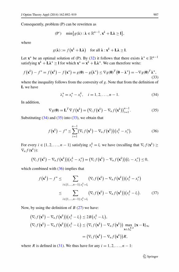
Consequently, problem (P) can be rewritten as
(P’) min{g(λ) : λ ∈ R
n−1,xk + Lλ ≥ l},
where
g(λ) := f(xk + Lλ
)for all λ : xk + Lλ ≥ l.
Let x∗ be an optimal solution of (P). By (32) it follows that there exists λ∗ ∈ Rn−1
satisfying xk + Lλ∗ ≥ l for which x∗ = xk + Lλ∗. We can therefore write:
f(xk
) − f ∗ = f(xk
) − f(x∗) = g(0) − g
(λ∗) ≤ ∇g(0)T
(0 − λ∗) = −∇g(0)T λ∗,
(33)where the inequality follows from the convexity of g. Note that from the definition ofL we have
λ∗i = x∗
i − xki , i = 1,2, . . . , n − 1. (34)
In addition,
∇g(0) = LT ∇f(xk
) = (∇if(xk
) − ∇nf(xk
))n−1i=1 . (35)
Substituting (34) and (35) into (33), we obtain that
f(xk
) − f ∗ ≤n−1∑
i=1
(∇if(xk
) − ∇nf(xk
))(xki − x∗
i
). (36)
For every i ∈ {1,2, . . . , n − 1} satisfying xki = li we have (recalling that ∇if (xk) ≥
∇nf (xk)):
(∇if(xk
) − ∇nf(xk
))(xki − x∗
i
) = (∇if(xk
) − ∇nf(xk
))(li − x∗
i
) ≤ 0,
which combined with (36) implies that
f(xk
) − f ∗ ≤∑
i∈{1,...,n−1}:xki >li
(∇if(xk
) − ∇nf(xk
))(xki − x∗
i
)
≤∑
i∈{1,...,n−1}:xki >li
(∇if(xk
) − ∇nf(xk
))(xki − li
). (37)
Now, by using the definition of B (27) we have:
(∇if(xk
) − ∇nf(xk
))(xki − li
) ≤ 2B(xki − li
),
(∇if(xk
) − ∇nf(xk
))(xki − li
) ≤ (∇if(xk
) − ∇nf(xk
))max
x∈�K,ln
‖x − l‖∞
= (∇if(xk
) − ∇nf(xk
))R,
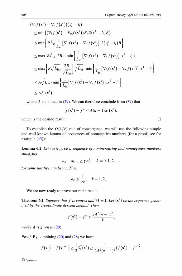
where R is defined in (31). We thus have for any i = 1,2, . . . , n − 1:
908 J Optim Theory Appl (2014) 162:892–919
(∇if(xk
) − ∇nf(xk
))(xki − li
)
≤ min{(∇if
(xk
) − ∇nf(xk
))R,2
(xki − li
)B
}
≤ min
{RLin
1
Lin
[∇if(xk
) − ∇nf(xk
)],2
(xki − li
)B
}
≤ max{RLin,2B} · min
{1
Lin
[∇if(xk
) − ∇nf(xk
)], xk
i − li
}
≤ max
{R
√Lin,
2B√
Lin
}√Lin · min
{1
Lin
[∇if(xk
) − ∇nf(xk
)], xk
i − li
}
≤ A
√Lin · min
{1
Lin
[∇if(xk
) − ∇nf(xk
)], xk
i − li
}
≤ AS1(xk
),
where A is defined in (29). We can therefore conclude from (37) that
f(xk
) − f ∗ ≤ A(n − 1)S1(xk
),
which is the desired result. �
To establish the O(1/k) rate of convergence, we will use the following simpleand well-known lemma on sequences of nonnegative numbers (for a proof, see forexample [43]):
Lemma 6.2 Let {ak}k≥0 be a sequence of nonincreasing and nonnegative numberssatisfying
ak − ak+1 ≥ γ a2k , k = 0,1,2, . . .
for some positive number γ . Then
ak ≤ 1
γ k, k = 1,2, . . .
We are now ready to prove our main result.
Theorem 6.1 Suppose that f is convex and M = 1. Let {xk} be the sequence gener-ated by the 2-coordinate descent method. Then
f(xk
) − f ∗ ≤ 2A2(n − 1)2
k,
where A is given in (29).
Proof By combining (20) and (28) we have
f(xk
) − f(xk+1) ≥ 1
2S2
1
(xk
) ≥ 1
2A2(n − 1)2
(f
(xk
) − f ∗)2.
J Optim Theory Appl (2014) 162:892–919 909
Therefore,
(f
(xk
) − f ∗) − (f
(xk+1) − f ∗) ≥ 1
2A2(n − 1)2
(f
(xk
) − f ∗)2.
Invoking Lemma 6.2 with ak := f (xk) − f ∗ and γ = 12A2(n−1)2 , the desired result
follows. �
Remark 6.1 It is not difficult to see that the proof of Lemma 6.1 can be refined andthe inequality (28) can be replaced with
f(xk
) − f ∗ ≤ A(‖xk − l‖0 − 1
)S1
(xk
),
where for a vector y, ‖y‖0 stands for the number of nonzero elements in y. Therefore,if for example the feasible set is the unit simplex and the sparsity of all the iteratesis bounded via ‖xk‖0 ≤ p, then f (xk) − f ∗ ≤ A(p − 1)S1(xk), and the complexityresult will be replaced by
f(xk
) − f ∗ ≤ 2A2(p − 1)2
k,
which is a significant improvement when p � n. This sparsity property is rathercommon in several applications such as the Chebyshev center problem, which willbe described in Sect. 7.1.
Remark 6.2 We note that for the dual SVM problem, an asymptotic linear rate ofconvergence was established in [44] under the assumption that Q is positive definiteand that strict complementarity holds at the optimal primal-dual solution. This re-sult was also used in order to show the asymptotic linear rate of convergence of thedecomposition method derived in [29], which exploits second order information inthe index selection strategy. Our objective here was to derive a nonasymptotic rate ofconvergence result, i.e., establish the fact that the accuracy of an iterative optimiza-tion algorithm can be guaranteed to hold from the first iteration and not only for alarge enough value of the iteration counter k.
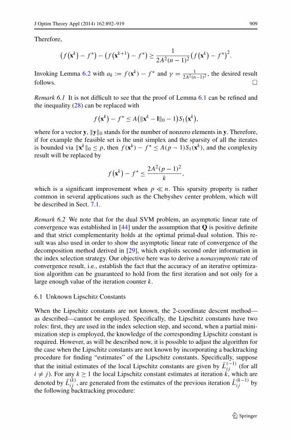
6.1 Unknown Lipschitz Constants
When the Lipschitz constants are not known, the 2-coordinate descent method—as described—cannot be employed. Specifically, the Lipschitz constants have tworoles: first, they are used in the index selection step, and second, when a partial mini-mization step is employed, the knowledge of the corresponding Lipschitz constant isrequired. However, as will be described now, it is possible to adjust the algorithm forthe case when the Lipschitz constants are not known by incorporating a backtrackingprocedure for finding “estimates” of the Lipschitz constants. Specifically, supposethat the initial estimates of the local Lipschitz constants are given by L
(−1)ij (for all
i �= j ). For any k ≥ 1 the local Lipschitz constant estimates at iteration k, which aredenoted by L
(k)ij , are generated from the estimates of the previous iteration L
(k−1)ij by
the following backtracking procedure:
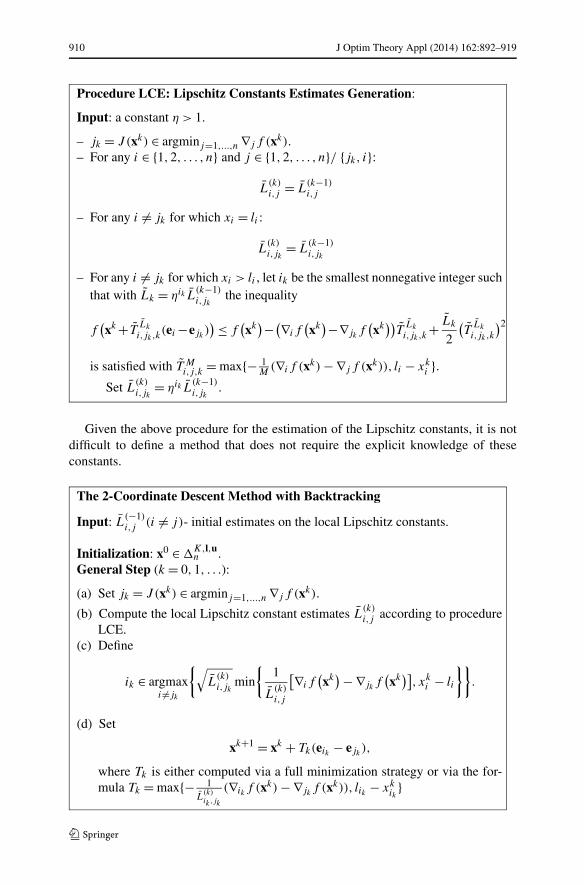
910 J Optim Theory Appl (2014) 162:892–919
Procedure LCE: Lipschitz Constants Estimates Generation:
Input: a constant η > 1.
– jk = J (xk) ∈ argminj=1,...,n ∇j f (xk).– For any i ∈ {1,2, . . . , n} and j ∈ {1,2, . . . , n}/ {jk, i}:
L(k)i,j = L
(k−1)i,j
– For any i �= jk for which xi = li :
L(k)i,jk
= L(k−1)i,jk
– For any i �= jk for which xi > li , let ik be the smallest nonnegative integer suchthat with Lk = ηik L
(k−1)i,jk
the inequality
f(xk + T
Lk
i,jk,k(ei −ejk
)) ≤ f
(xk
)−(∇if(xk
)−∇jkf
(xk
))T
Lk
i,jk,k+ Lk
2
(T
Lk
i,jk,k
)2
is satisfied with T Mi,j,k = max{− 1
M(∇if (xk) − ∇j f (xk)), li − xk
i }.Set L
(k)i,jk
= ηik L(k−1)i,jk
.
Given the above procedure for the estimation of the Lipschitz constants, it is notdifficult to define a method that does not require the explicit knowledge of theseconstants.
The 2-Coordinate Descent Method with Backtracking
Input: L(−1)i,j (i �= j)- initial estimates on the local Lipschitz constants.
Initialization: x0 ∈ �K,l,un .
General Step (k = 0,1, . . .):
(a) Set jk = J (xk) ∈ argminj=1,...,n ∇j f (xk).
(b) Compute the local Lipschitz constant estimates L(k)i,j according to procedure
LCE.(c) Define
ik ∈ argmaxi �=jk
{√L
(k)i,jk
min
{1
L(k)i,j
[∇if(xk
) − ∇jkf
(xk
)], xk
i − li
}}.
(d) Set
xk+1 = xk + Tk(eik − ejk),
where Tk is either computed via a full minimization strategy or via the for-mula Tk = max{− 1
L(k)ik ,jk
(∇ik f (xk) − ∇jkf (xk)), lik − xk
ik}

J Optim Theory Appl (2014) 162:892–919 911
The analysis of the above method is very technical, and is based on the analysisemployed in the known Lipschitz constants case. We will therefore state the mainconvergence result without a proof.
Theorem 6.2 Suppose that f is convex and M = 1. Let {xk} be the sequence gener-ated by the 2-coordinate descent method with backtracking. Then
f(xk
) − f ∗ ≤ max
{√ηLmaxR,
2B√
L(−1)min
}2
(n − 1)2 1
2k, k = 1,2, . . .
where
Lmax = maxi �=j
Li,j ,
L(−1)min = min
i �=jL
(−1)i,j .
7 Examples and Numerical Illustrations
In order to demonstrate the potential of the 2-coordinate descent methods described inthe paper, we give two illustrative examples and report several experiments on someSVM training problems. All the experiments are performed on the class of quadraticconvex objective functions for which the Lipschitz constant can be easily obtainedfrom the maximum eigenvalue of the Hessian matrix. We use the acronym 2cd forthe 2-coordinate descent method.
7.1 A Chebyshev Center Example
Given a set of points a1,a2, . . . ,am ∈ Rd , a known geometrical problem is to find
their Chebyshev center, which is the center of the minimum radius ball enclosing allthe points. There exist many algorithms for solving the Chebyshev center problem;see for example the paper [38], which also contains an overview of the problem aswell as many relevant references. Mathematically, the problem can be directly formu-lated as the following convex optimization problem (r stands for the squared radiusand x is the Chebyshev center):
minr∈R,x∈Rd
{r : ‖x − ai‖2 ≤ r, i = 1, . . . ,m
}, (38)
which is of course not of the form (P). However, a standard computation shows thatthe dual of (38) is of the form of problem (P) with a quadratic objective and a unitsimplex as the feasible set:
max
{
−‖Aλ‖2 +m∑
i=1
‖ai‖2λi : λ ∈ �m
}
, (39)
912 J Optim Theory Appl (2014) 162:892–919
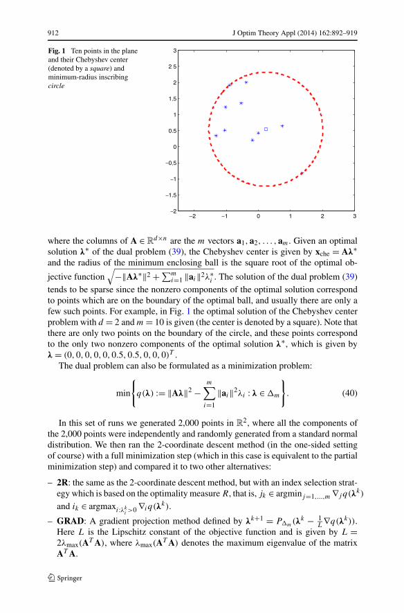
Fig. 1 Ten points in the planeand their Chebyshev center(denoted by a square) andminimum-radius inscribingcircle
where the columns of A ∈ Rd×n are the m vectors a1,a2, . . . ,am. Given an optimal
solution λ∗ of the dual problem (39), the Chebyshev center is given by xche = Aλ∗and the radius of the minimum enclosing ball is the square root of the optimal ob-
jective function√
−‖Aλ∗‖2 + ∑mi=1 ‖ai‖2λ∗
i . The solution of the dual problem (39)tends to be sparse since the nonzero components of the optimal solution correspondto points which are on the boundary of the optimal ball, and usually there are only afew such points. For example, in Fig. 1 the optimal solution of the Chebyshev centerproblem with d = 2 and m = 10 is given (the center is denoted by a square). Note thatthere are only two points on the boundary of the circle, and these points correspondto the only two nonzero components of the optimal solution λ∗, which is given byλ = (0,0,0,0,0,0.5,0.5,0,0,0)T .
The dual problem can also be formulated as a minimization problem:
min
{
q(λ) := ‖Aλ‖2 −m∑
i=1
‖ai‖2λi : λ ∈ �m
}
. (40)
In this set of runs we generated 2,000 points in R2, where all the components of
the 2,000 points were independently and randomly generated from a standard normaldistribution. We then ran the 2-coordinate descent method (in the one-sided settingof course) with a full minimization step (which in this case is equivalent to the partialminimization step) and compared it to two other alternatives:
– 2R: the same as the 2-coordinate descent method, but with an index selection strat-egy which is based on the optimality measure R, that is, jk ∈ argminj=1,...,m ∇j q(λk)
and ik ∈ argmaxi:λki >0 ∇iq(λk).
– GRAD: A gradient projection method defined by λk+1 = P�m(λk − 1L∇q(λk)).
Here L is the Lipschitz constant of the objective function and is given by L =2λmax(AT A), where λmax(AT A) denotes the maximum eigenvalue of the matrixAT A.

J Optim Theory Appl (2014) 162:892–919 913
Fig. 2 The resulting Chebyshev center and circle for different solvers
All the algorithms were initialized with the vector λ0 = e1 and ran for only 10iterations. In addition, we present the result of 100 iterations of the gradient projectionmethod; this experiment was denoted by GRAD(100). The resulting circles can beseen in Fig. 2.
We also ran CVX [45] with the SeDuMi solver [46] and found that the optimalradius is 3.6848 and the solution is extremely sparse—it has only three nonzero com-ponents in the optimal solution, which correspond to the three points on the boundaryof the resulting circle. As can be clearly seen in the four images, the best result wasobtained by the 2-coordinate descent method (top left image) with a radius of 3.7001.It can be seen in this image that there are three points on the border of the circle. Theresult of 2R is clearly worse (radius 3.9382), and the resulting circle is obviously notthe minimal one. The gradient projection method GRAD produced a circle which isvery far from the optimal one (radius 4.3819), and even when 100 iterations wereemployed, the result was not satisfactory.
7.2 A Random Example
Consider the quadratic minimization problem
min
{1
2xT Qx + bT x : x ∈ �100
},
914 J Optim Theory Appl (2014) 162:892–919
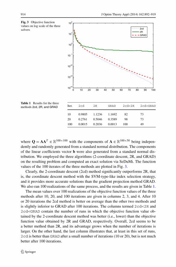
Fig. 3 Objective functionvalues on log scale of the threesolvers
Table 1 Results for the threemethods 2cd, 2R, and GRAD Iter. 2cd 2R GRAD 2cd<2R 2cd<GRAD
10 0.9805 1.1236 1.1692 82 73
20 0.2761 0.5046 0.3589 98 73
100 0.0015 0.2036 0.0013 100 49
where Q = AAT ∈ R100×100 with the components of A ∈ R
100×50 being indepen-dently and randomly generated from a standard normal distribution. The componentsof the linear coefficients vector b were also generated from a standard normal dis-tribution. We employed the three algorithms (2-coordinate descent, 2R, and GRAD)on the resulting problem and computed an exact solution via SeDuMi. The functionvalues of the 100 iterates of the three methods are plotted in Fig. 3.
Clearly, the 2-coordinate descent (2cd) method significantly outperforms 2R, thatis, the coordinate descent method with the SVM-type-like index selection strategy,and it provides more accurate solutions than the gradient projection method GRAD.We also ran 100 realizations of the same process, and the results are given in Table 1.
The mean values over 100 realizations of the objective function values of the threemethods after 10, 20, and 100 iterations are given in columns 2, 3, and 4. After 10or 20 iterations the 2cd method is better on average than the other two methods andis slightly inferior to GRAD after 100 iterations. The columns termed 2cd<2R and2cd<GRAD contain the number of runs in which the objective function value ob-tained by the 2-coordinate descent method was better (i.e., lower) than the objectivefunction value obtained by 2R and GRAD, respectively. Overall, 2cd seems to bea better method than 2R, and its advantage grows when the number of iterations islarger. On the other hand, the last column illustrates that, at least in this set of runs,2cd is better than GRAD after a small number of iterations (10 or 20), but is not muchbetter after 100 iterations.
J Optim Theory Appl (2014) 162:892–919 915
7.3 Experiments on SVM Training Problems
A well-known problem in classification is the problem of training a support vectormachine (SVM) in which one seeks to separate two sets of vectors (or their transfor-mations) by a hyperplane. The dual problem associated with the problem of trainingan SVM is given by the following convex quadratic programming problem (see [18,19, 21] for more details):
max
{n∑
i=1
αi − 1
2
∑
i,j
αiαj yiyj k(xi ,xj ) :n∑
i=1
αiyi = 0,0 ≤ αi ≤ C
}
, (41)
where the vectors x1, . . . ,xn ∈ Rd and their corresponding classes y1, . . . , yn ∈
{−1,1} are the given “training data” and k(·, ·) is called the kernel function; it isassumed that the matrix (k(xi ,xj ))i,j is positive semidefinite. Obviously, problem(41) is of the form of model (1), and indeed many of the methods developed tosolve it apply to this model, such as those in [19–24, 29, 40, 44]. In this sectionwe report the results of experiments conducted on some SVM training test problems.The problem that we actually solve is the dual-SVM problem (41). Before applyingthe algorithm, we transformed it into a problem over a double-sided simplex set bythe linear change of variables described in Sect. 2.1. Since the 2-coordinate descentmethod in the double-sided setting cannot handle large-scale problems, we used animplementable variant of the method, which we call 2cd-hybrid. The index selectionstrategy in the hybrid method is defined as follows: the index j is predetermined tobe chosen as in the maximum violation criteria (9), while the index i is chosen tomaximize the same term as in S2. Explicitly, this can be written as:
jk ∈ argminj :xj <uj
∇j f(xk
), (42)
ik ∈ argmaxi=1,...,n
{√Li,jk
min
{1
Li,jk
[∇if(xk
) − ∇jkf
(xk
)], xk
i − li , ujk− xk
jk
}}. (43)
Note that the index selection strategy coincides with the one-sided index selectionstrategy when the feasible set is indeed a one-sided simplex set. All the data sets havebeen taken from the LIBSVM database [47]. The problems that were tested alongwith their dimension are described below:
– a1a (n = 1605);– a4a (n = 4781);– mushrooms (n = 8124);– w5a (n = 9888);– w7a (n = 4692);
To evaluate the performance of the method cd-hybrid, we compared it to two other2-coordinate descent type methods that differ only in their index selection strategy:(1) the 2R method described in the Chebyshev center example, which is essentiallythe same as the SVMlight method with q = 2, although our implementation is proba-bly not as efficient as the implementation in LIBSVM [48], and (2) the method we call
916 J Optim Theory Appl (2014) 162:892–919
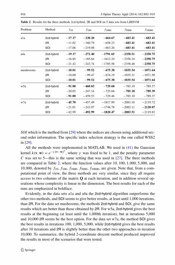
Table 2 Results for the three methods 2cd-hybrid, 2R and SOI on 5 data sets from LIBSVM
Problem Method f10 f100 f1000 f5000 f10000
a1a 2cd-hybrid −17.17 −230.20 −664.67 −683.41 −683.41
2R −11.02 −160.79 −658.23 −683.41 −683.41
SOI −17.06 −219.08 −663.26 −683.41 −683.41
a4a 2cd-hybrid −19.17 −272.40 −1791.65 −2358.51 −2358.75
2R −16.85 −185.64 −1612.24 −2358.34 −2358.75
SOI −21.42 −243.74 −1785.58 −2358.48 −2358.75
mushrooms 2cd-hybrid −10.01 −99.52 −675.38 −1035.54 −1071.64
2R −10.00 −99.47 −674.19 −1035.31 −1071.50
SOI −10.01 −99.52 −675.38 −1035.54 −1071.64
w5a 2cd-hybrid −91.00 −460.03 −729.68 −785.10 −789.37
2R −20.05 −247.14 −725.04 −785.18 −789.39
SOI −91.00 −459.53 −729.46 −785.10 −789.37
w7a 2cd-hybrid −45.70 −457.49 −1817.99 −2083.18 −2119.72
2R −21.01 −243.97 −1748.78 −2082.11 −2120.07
SOI −42.99 −492.99 −1820.47 −2083.51 −2119.83
SOI which is the method from [29] where the indices are chosen using additional sec-ond order information. The specific index selection strategy is the one called WSS2in [29].
All the methods were implemented in MATLAB. We used in (41) the Gaussiankernel k(v,w) = e−γ ‖v−w‖2
, where γ was fixed to be 1, and the penalty parameterC was set to 5—this is the same setting that was used in [27]. The three methodsare compared in Table 2, where the function values after 10,100,1,000,5,000, and10,000, denoted by f10, f100, f1000, f5000, f10000, are given. Note that, from a com-putational point of view, the three methods are very similar, since they all requireaccess to two columns of the matrix Q at each iteration, and in addition several op-erations whose complexity is linear in the dimension. The best results for each of theruns are emphasized in boldface.
Evidently, in the data sets a1a and a4a the 2cd-hybrid algorithm outperforms theother two methods, and SOI seems to give better results, at least until 1,000 iterations,than 2R. For the data set mushrooms, the methods 2cd-hybrid and SOI, give the sameresults which are better than those obtained by 2R. For w5a, 2cd-hybrid gives the bestresults at the beginning (at least until the 1,000th iteration), but at iterations 5,000and 10,000 2R seems be the best option. For the data set w7a, the method SOI givesthe best results in iterations 100, 1,000, 5,000, while 2cd-hybrid gives the best resultsafter 10 iterations and 2R is slightly better than the other two approaches in iteration10,000. To summarize, the hybrid 2-coordinate descent method produced improvedthe results in most of the scenarios that were tested.

J Optim Theory Appl (2014) 162:892–919 917
8 Conclusions
In this paper, we considered the problem of minimizing a continuously differentiablefunction with a Lipschitz continuous gradient over a single linear equality constraintand bound constraints. Based on new optimality measures, we were able to derivenew block descent methods that perform at each iteration an optimization procedureon two chosen decision variables. In the convex case, the main result is a nonasymp-totic sublinear rate of convergence of the function values. There are still several openand interesting research questions that can be investigated. First, can the analysis begeneralized to the interesting and general case, where the constraint set consists of anarbitrary number of equality constraints? This will require a generalization of boththe optimality measures, the index selection strategies and the convergence analysis.Second, the rate of convergence analysis is restricted to the one-sided setting, and ageneralization to the two-sided setting does not seem to be straightforward; therefore,the question that arises is: Does there exist another proof technique that will enable usto analyze this important setting as well? A final important open question is: Can thedependency of the efficiency estimate in the dimension of the problem (Theorem 6.1)be removed?
Acknowledgements I would like to thank the three anonymous reviewers for their useful commentsand additional references which helped to improve the presentation of the paper. This work was partiallysupported by ISF grant #25312 and by BSF grant 2008100.
References
1. Bertsekas, D.P., Tsitsiklis, J.N.: Parallel and Distributed Computation. Prentice-Hall, EnglewoodCliffs (1989)
2. Ortega, J.M., Rheinboldt, W.C.: Iterative Solution of Nonlinear Equations in Several Variables. Aca-demic Press, New York (1970)
3. Auslender, A.: Méthodes numériques pour la décomposition et la minimisation de fonctions non dif-férentiables. Numer. Math. 18, 213–223 (1971/72)
4. Auslender, A.: Optimisation. Méthodes Numériques, Maîtrise de Mathématiques et Applications Fon-damentales. Masson, Paris (1976)
5. Auslender, A., Martinet, B.: Méthodes de décomposition pour la minimisation d’une fonctionnellesur un espace produit. C. R. Acad. Sci. Paris Sér. A-B 274, A632–A635 (1972)
6. Bertsekas, D.P.: Nonlinear Programming, 2nd edn. Athena Scientific, Belmont (1999)7. Cassioli, A., Lorenzo, D.D., Sciandrone, M.: On the convergence of inexact block coordinate descent
methods for constrained optimization. Eur. J. Oper. Res. 231(2), 274–281 (2013)8. Cassioli, A., Sciandrone, M.: A convergent decomposition method for box constrained optimization
problems. Optim. Lett. 3(3), 397–409 (2009)9. Grippo, L., Sciandrone, M.: Globally convergent block-coordinate techniques for unconstrained opti-
mization. Optim. Methods Softw. 10, 587–637 (1999)10. Luo, T., Tseng, P.: Error bounds and convergence analysis of feasible descent methods: a general
approach. Ann. Oper. Reas. 46, 157–178 (1993)11. Powell, M.J.D.: On search directions for minimization algorithms. Math. Program. 4, 193–201 (1973)12. Luo, T., Tseng, P.: On the convergence of the coordinate descent method for convex differentiable
minimization. J. Optim. Theory Appl. (1992)13. Polak, E., Sargent, R.W.H., Sebastian, D.J.: On the convergence of sequential minimization algo-
rithms. J. Optim. Theory Appl. 14, 439–442 (1974)14. Sargent, R.W.H., Sebastian, D.J.: On the convergence of sequential minimization algorithms. J. Op-
tim. Theory Appl. 12, 567–575 (1973)
918 J Optim Theory Appl (2014) 162:892–919
15. Tseng, P., Yun, S.: A coordinate gradient descent method for nonsmooth separable minimization.Math. Program. 117, 387–423 (2009)
16. Nesterov, Y.: Efficiency of coordinate descent methods on huge-scale optimization problems (2010).CORE Discussion paper 2010/2
17. Beck, A., Tetruashvili, L.: On the convergence of block coordinate descent type methods. SIAM J.Optim. 23(2), 2037–2060 (2013)
18. Burges, C.J.C.: A tutorial on support vector machines for pattern recognition. Data Min. Knowl.Discov. 2, 121–167 (1998)
19. Platt, J.C.: Sequential minimal optimization: a fast algorithm for training support vector machines.In: Scholkopf, B., Burges, C.J.C., Smola, A.J. (eds.) Advances in Kernel Methods—Support VectorLearning, pp. 185–208. MIT Press, Cambridge (1999)
20. Keerthi, S., Gilbert, E.: Convergence of a generalized SMO algorithm for SVM. Mach. Learn. 46,351–360 (2002)
21. Keerthi, S.S., Shevade, S.K., Bhattacharyya, C., Murthy, K.R.K.: Improvements to Platt’s SMO algo-rithm for SVM classifier design. Neural Comput. 13(3), 637–649 (2001)
22. Joachims, T.: Making large-scale SVM learning practical. In: Scholkopf, B., Burges, C.J.C., Smola,A.J. (eds.) Advances in Kernel Methods—Support Vector Learning, B, pp. 169–184. MIT Press, Cam-bridge (1999)
23. Lin, C.J.: On the convergence of the decomposition method for support vector machines. IEEE Trans.Neural Netw. 12, 1288–1298 (2001)
24. Lin, C.J.: Asymptotic convergence of an SMO algorithm without any assumptions. IEEE Trans. Neu-ral Netw. 13, 248–250 (2002)
25. Palagi, L., Sciandrone, M.: On the convergence of a modified version of SVMlight algorithm. Optim.Methods Softw. 20(2–3), 317–334 (2005)
26. Lucidi, S., Palagi, L., Risi, A., Sciandrone, M.: A convergent hybrid decomposition algorithm modelfor SVM training. IEEE Trans. Neural Netw. 20(6), 1055–1060 (2009)
27. Lin, C.J., Lucidi, S., Palagi, L., Risi, A., Sciandrone, M.: Decomposition algorithm model for singlylinearly-constrained problems subject to lower and upper bounds. J. Optim. Theory Appl. 141(1),107–126 (2009)
28. Lucidi, S., Palagi, L., Risi, A., Sciandrone, M.: A convergent decomposition algorithm for supportvector machines. Comput. Optim. Appl. 38(2), 217–234 (2007)
29. Chen, P.H., Fan, R.E., Lin, C.J.: Working set selection using second order information for trainingsupport vector machines. J. Mach. Learn. Res. 6, 1889–1918 (2005)
30. Glasmachers, T., Igel, C.: Maximum-gain working set selection for SVMs. J. Mach. Learn. Res. 7,1437–1466 (2006)
31. Chang, C.C., Hsu, C.W., Lin, C.J.: The analysis of decomposition methods for support vector ma-chines. IEEE Trans. Neural Netw. 11, 1003–1008 (2000)
32. Dai, Y.H., Fletcher, R.: New algorithms for singly linearly constrained quadratic programs subject tolower and upper bounds. Math. Program., Ser. A 106(3), 403–421 (2006)
33. Serafini, T., Zanghirati, G., Zanni, L.: Gradient projection methods for quadratic programs and appli-cations in training support vector machines. Optim. Methods Softw. 20, 353–378 (2005)
34. Tseng, P., Yun, S.: A coordinate gradient descent method for linearly constrained smooth optimizationand support vector machines training. Comput. Optim. Appl. 47(2), 179–206 (2010)
35. Liuzzi, G., Palagi, L., Piacentini, M.: On the convergence of a Jacobi-type algorithm for singlylinearly-constrained problems subject to simple bounds. Optim. Lett. 5(2), 347–362 (2011)
36. Markowitz, H.: Portfolio selection. J. Finance 7, 77–91 (1952)37. Bomze, I.M.: Evolution towards the maximum clique. J. Glob. Optim. 10(2), 143–164 (1997)38. Xu, S., Freund, R.M., Sun, J.: Solution methodologies for the smallest enclosing circle problem.
Comput. Optim. Appl. 25(1–3), 283–292 (2003). A tribute to Elijah (Lucien) Polak39. Lin, C.J.: A formal analysis of stopping criteria of decomposition methods for support vector ma-
chines. IEEE Trans. Neural Netw. 13(5), 1045–1052 (2002)40. Hush, D., Scovel, C.: Polynomial-time decomposition algorithms for support vector machines. Mach.
Learn. 51(1), 51–71 (2003)41. Beck, A., Teboulle, M.: Gradient-based algorithms with applications to signal recovery problems.
In: Eldar, Y., Palomar, D. (eds.) Convex Optimization in Signal Processing and Communications.Cambridge University Press, Cambridge (2010)
42. Nesterov, Y.: Introductory Lectures on Convex Optimization. Kluwer, Boston (2004)43. Polyak, B.T.: Introduction to Optimization. Translations Series in Mathematics and Engineering. Op-
timization Software, New York (1987)

J Optim Theory Appl (2014) 162:892–919 919
44. Chen, P.H., Fan, R.E., Lin, C.J.: A study on SMO-type decomposition methods for support vectormachines. IEEE Trans. Neural Netw. 17(4), 893–908 (2006)
45. Grant, M., Boyd, S.: CVX: Matlab software for disciplined convex programming, version 1.21.http://cvxr.com/cvx (2011)
46. Sturm, F.J.: Using SeDuMi 1.02, a Matlab toolbox for optimization over symmetric cones. Optim.Methods Softw. 11–12, 625–653 (1999)
47. Chang, C.C., Lin, C.J.: LIBSVM data: Classification, regression, and multi-label. http://www.csie.ntu.edu.tw/~cjlin/libsvmtools/datasets/
48. Chang, C.C., Lin, C.J.: LIBSVM: a library for support vector machines. ACM Trans. Intell. Syst.Technol. 2(3), 1–27 (2011). Software available at http://www.csie.ntu.edu.tw/~cjlin/libsvm