TEZA DE ABILITARE

DR. RADU PURICE

OCTOMBRIE 2013

INSTITUTUL DE MATEMATICA “SIMION STOILOW” AL ACADEMIEI ROMANE

CALEA GRIVITEI NR. 21, 010702, BUCURESTI, ROMANIA Tel: +40 21 319 65 06; Fax: +40 21 319 65 05

SUMMARYAfter the defence of my PhD thesis in 1990 I have continued to investigate several as-

pects concerning the mathematical description of different quantum systems, publishing over40 scientific papers either in mathematical journals or in books or proceedings of internationalconferences. My interest has focussed on the basic mathematical structures and concepts in-volved in the mathematical description of the qualitative behaviour of the quantum systems, inorder to contribute to the elaboration of a complete and coherent mathematical understandingof this class of physical systems. The main directions involved in this research have been: thetheory of unbounded linear operators in Hilbert spaces, the theory of elliptic differential oper-ators, the pseudodifferential calculus, the theory of local convex spaces, harmonic analysis andthe theory of operator algebras.

In a first period, I have studied the method of positive commutators for a detailed spectralanalysis of differential and pseudodifferential operators. The idea of using positive commuta-tors in spectral analysis, by defining H-smooth operators, originated in the papers of Putnam[145] and Kato [102] and was largely developed by Lavine[113], [114], [115]. Much later, Mourre[135] pointed out the idea of a ”conjugate operator” which requires considerably weaker posi-tivity or regularity conditions. The abstract nature of the method elaborated by Mourre andlargely developed in [100], [144], [68], [6] and many others, has a wide range of applications,starting with quantum Hamiltonians of very different kinds: various two-body systems, N-bodyHamiltonians, long-range perturbations, random potentials and continuing with propagation ofwaves, Laplace operators on non-compact manifolds and many others. This method providesmainly four types of information: discreteness of the pure point spectrum on given intervals;absence of singularly continuous spectrum; control of the boundary values of the resolvent onthe real axis (the so-called Limiting Absorption Principle) and existence and completeness forthe wave operators associated to a given pair of operators for which the difference satisfiessome regularity condition and some ”short-range” type behaviour at infinity. In [29, 30, 94, 36]we have proposed some conjugate operators that provide good commutator inequalities withsome classes of quantum Hamiltonians (like perturbed Dirac operators, Schrodinger operatorswith short-range magnetic fields and N-body Hamiltonians with short-range magnetic fields).Using then the abstract version of the commutator method from [6] we have obtained LimitingAbsorption Principles and detailed spectral properties for these classes of operators.

In [123, 124, 125, 130], in collaboration with Marius Mantoiu, we have obtained a classof weighted, Hardy type estimations, starting from commutator estimations and used theseweighted estimations in order to obtain decay properties of eigenfunctions of some pseudodif-ferential operators. We obtained among other things a generalization of Theorem 14.5.2 in [85]and of Theorem 30.2.9 in [87], for non-local convolution operators and exponential weights.

In the period 1998 - 2004, together with Marius Mantoiu we have studied the recent researchdirection opened by some papers by Vladimir I. Georgescu and his co-workers (mainly [71, 56,72]) and by the paper [15] by Jean Bellissard proposing methods from the theory of C∗-algebrasfor the study of the essential spectrum of very large classes of quantum Hamiltonians. Thismethod was based on the very natural connection between the essential spectrum and the”localizations at infinity” for a pseudodifferential operator and on a cross-product structure ofthe C∗-subalgebra to which the given operator may be affiliated. In this context, in [7] we haveintroduced some operator ideals strictly containing the compact operators, and we have usedthem in order to obtain very general ”non-propagation” theorems. The idea of using twistedcrossed-products in order to deal with Hamiltonians with magnetic fields lead us to put intoevidence a ”twisted Weyl system” and a ”twisted” pseudodifferential calculus associated to it,

1

that allowed us to develop a magnetic quantization to which we have devoted a large part ofthe following papers [127, 128, 90, 92, 131, 132, 133, 96]. Applying this calculus to differentmodels and problems is my main concern for the near future.

In [121] we consider a two dimensional Hamiltonian with a magnetic field depending onlyon one of the two spatial variables, introduced in [97], and obtain some detailed propagationestimations for its evolution.

Another research direction, suggested by Gheorghe Nenciu, started from a problem left openin the study presented in [141]: the completeness of the wave operators for a Dirac Hamiltonianwith a time dependent potential defined as the solution of the free Maxwell equations withregular and compactly supported initial data. This problem is of interest in connection withthe study of the Dirac Quantum Field in interaction with an external electromagnetic field. Itcan be shown [164] that if the ”one-particle ” scattering matrix exists and satisfies a specialproperty, then the scattering matrix for the quantum field also exists and can be computed bythe second quantization procedure. This problem is considered in [P] but only partial results areobtained and nothing is said concerning the completeness of the ”one-particle” wave operators.In [33, 35] we prove that the wave operators exist and are unitary for specific initial values ofthe solutions of the Maxwell equations. Related to this research direction is also our paper [34]in which we generalize the results of [45] to the case of perturbations that do not preserve theoperator domain and can be defined only in the sense of sums of quadratic forms.

In our papers [49, 50] we have addressed the description of the currents that characterizesome classes of non-equilibrium stationary states in quantum statistical mechanics. More pre-cisely we have considered the problem of computing the current through a small system as thetime derivative of the charge operator averaged in a non-equilibrium steady state of the systemcoupled to a number of reservoirs (leads) at different values of the chemical potential. Weconsider that at t = −∞ the full system is in a Gibbs equilibrium state at a given temperatureand chemical potential. Then we adiabatically turn on a potential bias between the leads,modelling in this way a gradual appearance of a difference in the chemical potentials. Thestatistical density matrix is found as the solution of a quantum Liouville equation. The currentcoming out of a given lead is defined to be the time derivative at t = 0 of its mean charge.Then one performs the linear response approximation with respect to the bias thus obtaininga Kubo-like formula [24], and finally the thermodynamic and adiabatic limits. The currentis given by the Landauer-Buttiker formula, specialized to the linear response case. Note thatthe perturbation introduced by the electrical bias is not spatially localized (as in other casesexisting in the literature), and this makes the adiabatic limit for the full state (i.e. without thelinear response approximation) rather difficult. In [49] we greatly improve the method of proofof [51], which also allows us to extend the results to the continuous case. In [50] we deal withthe rigorous construction of the adiabatic non-equilibrium state.

Most of my research activity has been done in collaboration with colleagues from IMAR,University of Geneva, University Paris 6, CPT-Marseille, University of Aalborg and Universityof Chile at Santiago de Chile. Let me also point out that the PhD thesis of Dr. Max Leinat the Technische Universitat Munchen, under the supervision of Prof. Herbert Spohn, anddealing with an application of the ’twisted’ pseudodifferential calculus developed by our team inBucharest, has been elaborated also under my partial supervision. The same is true concerningthe PhD thesis of Dr. Nassim Athmouni at the University of Sfax (Tunisia), under the commonsupervision of Prof. Mondher Damak and myself. In the last years I have been invited to givelecture series for PhD students at the Universities of Aalborg, Santiago de Chile and Tunis.

2

REZUMATDupa sustinerea Tezei de Doctorat in 1990 am continuat cercetarile mele privind descrierea

matematica a diferitelor sisteme cuantice, publicand peste 40 de lucrari stiintifice atat in revistede matematica cat si in carti sau in proceeding-uri ale unor conferinte internationale. Interesulmeu s-a axat asupra structurilor matematice de baza si asupra conceptelor implicate de fun-damentarea matematica a descrierii calitative a sistemelor cuantice, avand ca scop intelegereamatematica completa si coerenta a acestei clase de sisteme fizice. Principalele directii implicatein aceasta cercetare au fost: teoria operatorilor lineari nemarginiti in spatii Hilbert, teoria op-eratorilor diferentiali eliptici, calculul pseudodiferential, teoria spatiilor local convexe, analizaarmonica si teoria algebrelor de operatori.

Intr-o prima perioada am studiat metoda comuntatorilor pozitivi pentru analiza spectraladetaliata a operatorilor diferentiali si pseudodiferentiali. Ideia folosirii comutatorilor pozitiviin analiza spectrala, prin introducerea clasei operatorii H-netezi, are la origine lucrarile luiPutnam [145] si Kato [102] si a fost dezvoltata pe larg de catre Lavine [113, 114, 115]. Multmai tarziu, Mourre [135] a emis ideia unui operator conjugat care implica conditii considerabilmai slabe de regularitate si de pozitivitate. Natura abstracta a metodei elaborate de Mourresi mult dezvoltata apoi in lucrarile [100], [144], [68], [6]], precum si multe altele, are un largdomeniu de aplicatii, incepand cu Hamiltonienii cuantici de diferite feluri: diferite sisteme de 2corpuri, Hamiltonieni de N corpuri, perturbatii cu raza lunga, potentiale aleatoare si continuandcu propagarea undelor, oparatorii Laplace pe varietati necompacte si multe altele. Aceasatmetoda aduce in principal patru tipuri de informatiI: discretitudinea spectrului pur punctualpe anumite intervale; absenta spectrului singular continuu; controlul valorilor la frontiera alrezolventelor pe axa reala (asa numitul principiu de absorbtie limita (Limiting AbsorptionPrinciple) si existenta si completitudinea operatorilor de unda asociati unei perechi date deoperatori pentru care diferenta satisface unele conditii de regularitate si o comportare de tip”short-range” la infinit. In lucrarile [29, 30, 94, 36] am propus operatori conjugati care sa asigureinegalitati de comutatori bune cu unele clase de Hamiltonieni cuantici (cum ar fi operatorii Diracperturbati, operatorii Schrdingerc in camp magnetic de tip ”short range” si Hamiltonieni de Ncorpuri in camp magnetic de tip ”short range”. Folosind astfel versiunea abstracta a metodeicomutatorilor din [6] am obtinut principii de absorbtie limita (Limiting Absorption Principles)si apoi proprietati spectrale detaliate pentru aceste clase de operatori.

In lucrarile [123, 124, 125, 130], in colaborare cu Marius Mantoiu, am obtinut o clasa deestimari de tip Hardy ponderate, pornind de la estimari pe comutatori si le-am folosit pentru aobtine proprietati de descrestere ale functiilor proprii ale unor operatori pseudodiferentiali. Pelanga alte lucruri, am obtinut o generalizare a teoremei 14.5.2 din [85] si a teoremei 30.2.9 din[87], pentru operatori nelocali de convolutie si ponderi exponentiale.

In perioada 1998-2004, impreuna cu Marius Mantoiu, am studiat directiile noi de cercetaredeschise de lucrarile lui Vladimir I. Georgescu si colaboratorii (in special [71, 56, 72]) si delucrarea lui Jean Bellissard [15] ce propuneau metode din teoria C∗-algebrelor pentru studiulspectrului esential al unor clase foarte mari de Hamiltonieni cuantici. Aceasta metoda sebazeaza pe o legatura foarte naturala intre spectrul esential si localizarile la infinit pentruun operator pseudodiferential si pe structura de produs incrucusat a unor sub C∗-algebre lacare operatorul dat poate fi afiliat. In acest context, in lucrarea [7] am introdus niste idealede operatori ce contin strict operatorii compacti si le-am folosit pentru a obtine teorme foartegenerale de nepropagare. Ideea de a utiliza structura de produs incrucisat ’torsionat’ pentrustudiul hamiltonienilor cuantici in camp magnetic ne-a condus la punerea in evidenta a unuisistem Weyl ’torsionat’ si al unui calcul pseudo-diferential ’torsionat’ asociat lui, care ne-a

3

permis sa dezvoltam o cuantificare magnetica, subiect caruia i-am dedicat o mare parte dinurmatoarele lucrari [127, 128, 90, 92, 131, 132, 133, 96]. Aplicarea acestui calcul la diferitemodele si probleme este principalul scop pe care mi l-am propus in viitorul apropiat. In lucrarea[121], consideram un Hamiltonian in doua dimensiuni, cu un camp magnetic dependent doarde una dintra variabilele spatiale, model introdus in [97] si obtinem unele estimari detaliate depropagare pentru evolutia sa.

O alta directie de cercetare sugerata de Gheorghe Nenciu a pornit de la o problema ramasadeschisa in studiul prezentat in lucrarea [141] si anume completitudinea operatorilor de undapentru un hamiltonuian Dirac cu un potential dependent de timp, definit ca solutie a ecuatiilorMaxwell libere cu date initiale avand anumite proprietati de de regularitate si descrestere .Aceasta problema este de interes pentru studiul camplului Dirac cuantic in interactie cu uncamp electromagnetic extern. Se poate arata [164] ca daca exista matricea de imprastiere uni-particula si daca satisface o anumita proprietate speciala, atunci exista de asemenea si matriceade imprastiere pentru campul cuantic si ea poate fi calculata prin procedura standard de a douacuantificare. Aceasta problema este considerata in [141], insa se obtin doar rezultate partialesi nu se spune nimic in ceea ce priveste completitudinea operatorului de unda uniparticula. Inlucrarile [33, 35] demonstram ca operatorii de unda exista si sunt unitari pentru valori initialespecifice ale ecuatiilor lui Maxwell. In cadrul aceastei directii de cercetare se inscrie si articolulnostru [34], in care generalizam rezultatele obtinute in [45] pentru cazul perturbatiilor care nupastreaza domeniul operatorului si pot fi definite doar in sensul sumei de forme patratice.

In lucrarile noastre [49, 50] ne-am ocupat de descriera curentilor ce caracterizeaza unele clasede stari stationare de neechilibru in mecanica statistica cuantica. Mai precis am consideratcalcularea curnetului printr-un sistem ”mic”, ca derivata in raport cu timpul a operatoruluide saracina mediat pe o stare stationara de neechilibru cuplat cu un numar de rezervoare ladiferite valori ale potentialului chimic. Am considerat ca la t = −∞ intregul sistem este intr-ostare de echilibru Gibbs la o temperatura si la un potetial chimic date. Apoi, am considerato introducere adiabatica a unei diferente de potential intre rezervoare, modeland in acest fel oaparitia graduala a unei diferente de potential chimic. Curentul ce iese dintr-un conductor dat,este definit ca fiind derivata in raport cu timpul la t = 0 a sarcinii sale medii. In continuare sestudiaza doar aproximarea de raspuns linear in functie de diferenta de potential, si se obtineastfel o formula de tip Kubo [24] si se studiaza in final limitele termodinamica si adiabatica.Pentru curent se obtine o formula de tip Landauer-Buttiker specifica aproximatiei de raspunslinear. Este de notat faptul ca perturbatia introdusa de diferenta de potential electric nu estelocalizata spatial (ca in alte cazuri existente in literatura) si aceasta face ca limita adiabaticaa starii (i.e fara aproximarea de raspuns linear) sa fie o problema destul de dificila. In lucrarea[49] am imbunatatit in mod considerabil metoda de demonstratie din [51] care ne permite deasemenea sa extindem rezultatele la cazul continuu. In lucrarea [50] ne ocupam de constructiariguroasa a starii de neechilibru in limita adiabatica.

Cea mai mare parte a activitatii mele de cercetare a fost facuta in colaborare cu colegiide la IMAR, Universitatea din Geneva,Universitatea Paris 6, CPT-Marsilia, Universitate dinAalborg si Universitatea de Chile din Santiago de Chile. As vrea de asemenea sa subliniez cateza de doctorat a Dr. Max Lein de la Technische Universitat din Munchen, de sub conducereaProf. Herbert Spohn si care se ocupa de o aplicatie a calculului pseudiferential ’torsionat’dezvoltata de grupul nostru de la Bucuresti, a fost eloaborata sub partiala mea coordonare. Lafel si teza de doctorat a Dr. Nassim Athmouni de la Universitatea din Sfax (Tunisia), elaboratasub supervizarea comuna a Prof. Mondher Damak si a mea. In ultimii ani, am fost invitat satin o serie de cursuri pentru studetii aflati la doctorat la Universitatile din Aalborg, Santiago

4

de Chile si Tunis.

5

In my thesis I make explicit use of existing printed materials from my ownreview papers and from my original research papers specifying each time the exactreferences.

Part I

The Research ActivityAfter the defence of my PhD thesis in 1990, dealing with some mathematical aspects in thequantum field theory, I have continued to investigate several aspects concerning the mathe-matical description of different quantum systems, publishing a number of 43 scientific paperseither in mathematical journals or in books or proceedings of international conferences. Withone exception, these papers may be considered as belonging to four main directions of research:

1. the conjugate operator method in spectral analysis;

2. some propagation properties for the Dirac operator;

3. the mathematical description of quantum systems in magnetic fields;

4. the study of non-equilibrium steady states for some classes of quantum systems.

1 An abstract non-propagation result

The paper [7] remains somehow outside the above classification. In fact, in the period 1998- 2004, together with Marius Mantoiu we have studied the recent research direction openedby some papers by Vladimir I. Georgescu and his co-workers (mainly [71, 56, 72]) and by thepaper [15] by Jean Bellissard proposing methods from the theory of C∗-algebras for the studyof the essential spectrum of very large classes of quantum Hamiltonians. This method wasbased on the very natural connection between the essential spectrum and the ”localizations atinfinity” for a pseudodifferential operator and on a cross-product structure of the C∗-subalgebrato which the given operator may be affiliated. In this context, in [7] we have introduced someoperator ideals strictly containing the compact operators, and we have used them in order toobtain very general ”non-propagation” theorems. The idea of using twisted crossed-productsin order to deal with Hamiltonians with magnetic fields lead us to put into evidence a ”twistedWeyl system” and a ”twisted” pseudodifferential calculus associated to it, that allowed us todevelop a magnetic quantization to which we have devoted a large part of the following papers.

But let me come back to [7] and briefly describe the main result we have proved; I am usingprinted materials from [7].

We start our analysis from operators of the form H = −∆ + V acting in L2(Rn), withpotentials V having different asymptotics in different directions, generalizing the situationstudied by Brian E. Davies and Barry Simon in [57]. Typically the potential V to be consideredis an element of a C*-algebra A of bounded, continuous functions on Rn. The functions in A arecharacterized by a specific asymptotic behaviour (for example asymptotic periodicity in certaincones). Then, by invoking the Neumann series for (H − z)−1 (which is convergent for =z large

6

enough), one finds that the resolvent of the operator H = −∆ + V belongs to a C*-algebraCA generated by products of elements of A (viewed as multiplication operators in L2(Rn)) andsuitable functions of momentum. We shall say that H is affiliated to CA. A central concept isthat of the essential spectrum of H relative to an ideal K of CA of the form K = CK, where Kis an ideal of A and CK is defined similarly to CA (just replace A by K in the definition of CA).Let us denote this spectrum by σK(H) and call it the essential spectrum associated with theideal K, (a precise definition is given below). For K = 0, σK(H) is the usual spectrum of H;for K = C0(Rn) (the space of continuous functions converging to zero at infinity), K will be theideal of compact operators and σK(H) the essential spectrum σess(H) of H. For an ideal K ofA such that C0(Rn) ⊂ K, σK(H) is a subset of σess(H). A typical non-propagation result willassert that scattering states of H with spectral support disjoint from σK(H) will essentiallynever be localized in certain spatial domains W determined by K. Using the essential spectrumassociated with such ideals to characterize some geometric properties for quantum Hamiltoniansseems to be new, although in the literature ideals have been used in connection with spectraltheory.Definition 1.0.1. (a) An observable affiliated to a C*-algebra C is a ∗-homomorphism fromthe C*-algebra C0(R) to C (i.e. a linear mapping Φ : C0(R) → C satisfying Φ(ξη) = Φ(ξ)Φ(η)and Φ(η)∗ = Φ(η) if ξ, η ∈ C0(R)).

(b) The spectrum σ(Φ) of the observable Φ is defined as the set of real numbers λ such thatΦ(η) 6= 0 whenever η(λ) 6= 0. σ(Φ) is a closed subset of R.

Now let K be a (closed, self-adjoint, bilateral) ideal in C. We denote by C ≡ C/K theassociated quotient C*-algebra and by Π the canonical ∗-homomorphism of C onto C. If Φ isan observable affiliated to C, then clearly Π Φ determines an observable affiliated to C.Definition 1.0.2. The spectrum σ(Π Φ) of the observable Π Φ (relative to C) is called theK-essential spectrum of Φ and will be denoted by σK(Φ): σK(Φ) ≡ σ(ΠΦ). Equivalently, a realnumber λ belongs to σK(Φ) if and only if Φ(η) /∈ K whenever η ∈ C0(R) is such that η(λ) 6= 0.

If Y is a locally compact, Hausdorff space, we denote by Cb(Y ) the abelian C*-algebra ofall bounded, continuous complex functions defined on Y . If G is a closed subset of Y , we setCG(Y ) = ϕ ∈ Cb(Y ) | ϕ(y) = 0, ∀y ∈ G. Certain C*-subalgebras of Cb(Y ) will be importantfurther on, in particular the algebras Cu

b (Y ) and C0(Y ) consisting respectively of all bounded,uniformly continuous functions and of all continuous functions vanishing at infinity. In factC0(Y ) is an ideal of Cb(Y ). We set X = Rn. Let Y be as above and assume that X acts on Yas a group of homeomorphisms: so if αx denotes the homeomorphism in Y associated with theelement x ∈ X, we have αxαx′ = αx+x′ . The mapping X×Y 3 (x, y) 7→ αx(y) ∈ Y is assumedcontinuous. Then α induces a representation of the group X by ∗-automorphisms of Cb(Y ) aswell as of various C*-subalgebras of Cb(Y ): for ϕ ∈ Cb(Y ) and x ∈ X, define ax(ϕ) ∈ Cb(Y ) by[ax(ϕ)](y) = ϕ(αx(y)) (y ∈ Y ).

Let A be a unital C*-subalgebra of Cb(X) containing C0(X). We denote its character spaceΩ(A) by X and we recall that X is a compactification of X, i.e. X is a compact topologicalspace and there is a homeomorphism i from X to a dense subset of X . For x ∈ X, the characteri(x) is given by the formula [i(x)](ϕ) = ϕ(x), for ϕ ∈ A. We write Z = X \ i(X) and call itthe frontier of X in X . By the Gelfand Theorem, A is isomorphic to the C*-algebra C(X ) ofcontinuous functions on Ω(A). We shall use the notation G : C(X )→ A for the inverse of theGelfand isomorphism. The C*-subalgebra CZ(X ) (consisting of continuous functions on X thatvanish on the frontier Z of X ) can be naturally identified with C0(X). There is a one-to-onecorrespondence between (self-adjoint, closed) ideals K of A and closed subsets G of X , givenby K = GCG(X ). In particular each closed subset F of the frontier Z determines an ideal KF

7

in A, viz. KF = GCF (X ). It is clear that such an ideal contains C0(X). Suppose now that theC*-algebra A considered above is contained in Cu

b (X) and invariant under translations. SinceA ⊂ Cu

b (X), the mapping x 7→ ax(ϕ) is norm continuous for each ϕ ∈ A. Furthermore theaction of X on itself (given as αx(y) = x + y) induces a continuous representation ρ of X byhomeomorphisms of the character space X = Ω(A): for τ ∈ X the character ρxτ is defined as[ρxτ ](ϕ) = τ [ax(ϕ)]. For y ∈ X, set τy = i(y); then ρxτy = τx+y (x ∈ X).

We consider some C*-subalgebras of the space B(H) of all bounded, linear operators in theHilbert space H = L2(X). If ϕ : X → C is a bounded, measurable function, we denote by ϕ(Q)the operator of multiplication by ϕ in H and by ϕ(P ) the operator F∗ϕ(Q)F (the operatorof multiplication by ϕ in the momentum space), where F is the Fourier transformation. AC*-subalgebra A of Cu

b (X) will be identified with the subalgebra of B(H) consisting of allmultiplication operators ϕ(Q) with ϕ ∈ A.

If A is a C*-subalgebra of Cbu(X), we write CA for the norm closure in B(H) of the set of

finite sums of the form ϕ1(Q)ψ1(P ) + · · · + ϕN(Q)ψN(P ) with ϕk ∈ A and ψk ∈ C0(X). Wemention the fact that, if A = C0(X), then CA is the ideal of all compact operators in L2(X).

If A is invariant under translations, then CA is a C*-algebra isomorphic to the crossedproduct algebra AoX defined in terms of the action ax of X on A. We use the following resultfrom the theory of crossed products: If K is an ideal in A that is invariant under translations,then the quotient C*-algebra CA/CK is isomorphic to [A/K]oX. The point is that the generaltheory allows us to define the crossed product [A/K]oX only by using the continuous action ofX by ∗-automorphisms of A/K (the quotient action); the fact that A/K is not a C*-subalgebraof B(H) does not matter.

Framework. A is a unital C*-subalgebra of Cub (X), invariant under translations and such

that C0(X) ⊂ A, and CA is the associated C*-subalgebra of B(H) introduced above (withH = L2(X)). X = Ω(A) is the character space of A, F a translation invariant, closedsubset of Z = X \ i(X) and CF (X ) the ideal in C(X ) determined by F . We set KF ≡GCF (X ), which is a translation invariant ideal in A. Then KF ≡ CKF is an ideal in CAthat contains all the compact operators in H.

Then, our main result is the following.Theorem 1.0.3. Let A and F be as in the Framework and let WWW be a filter base in X that isadjacent to F . Let H be a self-adjoint operator in H affiliated to CA. Let ε > 0 and η ∈ C0(R)with supp(η) ∩ σKF (ΦH) = ∅. Then there is a W ∈WWW such that

‖ χW (Q)η(H) ‖≤ ε.

Corollary 1.0.4. Let A, F , WWW and H be as in the Theorem. Then for each ε > 0 and eachη ∈ C0(R) with suppη ⊂ R \ σKF (ΦH), there exists W ∈WWW such that

‖ χW (Q)e−itHη(H)f ‖≤ ε ‖ f ‖

for all t ∈ R and all f ∈ L2(X).In [7] we give a number of examples of anisotropic problems as described above, having an

interesting physical interpretation and generalizing the results of [57].

8

I shall divide the rest of this part of the thesis in 4 sections devoted to the above 4 researchsubjects that I have developed in my scientific publications.

2 The Conjugate Operator Method in Spectral Analysis

I shall begin by presenting the main ideas of this method, some of its applications in spec-tral analysis of quantum Hamiltonians and some of the developments made by me and somecollaborators. I shall use the text in the introduction to [36].

The idea of using positive commutators in spectral analysis, by defining H-smooth oper-ators originated in the papers of Putnam [145] and Kato [102] and was largely developed byLavine[113], [114], [115]. Much later, Mourre [135] pointed out the idea of a ”conjugate opera-tor” which requires considerably weaker positivity or regularity conditions.

A specific feature of Mourre’s method is the use of a differential inequality which necessitatessome control on the second commutator of the operator with its conjugate; this kind of regularityhypothesis is to be found in all applications of the method. The abstract nature of the methodelaborated by Mourre and largely developed in [100], [144], [68] and many others, has a widerange of applications, starting with quantum Hamiltonians of very different kinds: varioustwo-body systems, N-body Hamiltonians, long-range perturbations, random potentials andcontinuing with propagation of waves, Laplace operators on non-compact manifolds and manyothers. This method provides mainly four types of information:

1. discreteness of the pure point spectrum on given intervals;

2. absence of singularly continuous spectrum;

3. control of the boundary values of the resolvent on the real axis (the so-called LimitingAbsorption Principle);

4. existence and completeness for the wave operators associated to a given pair of operatorsfor which the difference satisfies some regularity condition and some ”short-range” typebehaviour at infinity.

Let us make some comments upon the Limiting Absorption Principle for a self-adjointoperator H in a Hilbert space H. If we denote:

C± := z ∈ C | ±Imz > 0 (2.0.1)

then the function z 7−→ (H − z)−1is well defined, takes its values in the space of boundedoperators in H and is holomorphic separately on C+ and on C−, with respect to the operatornorm topology, but surely diverges when one approaches the spectrum of H. Suppose there isa Banach space E continuously and densely embedded in H, i.e. there is given a continuousinjection: E → H with dense image, so that at the algebraic level we may consider E alinear subspace of H equipped with a finer topology than that induced from H. IdentifyingH to its antidual by means of the Riesz lemma, we obtain a continuous injection with denserange: H → E∗ where E∗ is the adjoint of E . Let us denote by B(H;K) the linear spaceof bounded linear operators from the Banach space H to the Banach space K and we denoteB(H) := B(H;H). Then we have an obvious inclusion: B(H) ⊂ B(E ; E∗). Proving a ”limitingabsorption principle” consists in identifying a subset S of the absolutely continuous part of the

9

spectrum of H (as large as possible) and a Banach space E continuously and densely embeddedin H (also as large as possible) such that the two holomorphic applications:

C± 3 z 7−→ (H − z)−1 ∈ B(H) ⊂ B(E ; E∗) (2.0.2)

extend to two continuous applications:

C± ∪ S 3 z 7−→ (H − z)−1 ∈ B(E ; E∗). (2.0.3)

with (H − x− i0)−1 the limit at x ∈ S coming from C+ and (H − x+ i0)−1coming from C−.Usually we have continuity with respect to the weak∗ topology of B(E ; E∗) , that means thatfor any ϕ and ψ in E , the applications:

C± ∪ S 3 z 7−→< ϕ, (H − z)−1ψ >∈ C (2.0.4)

are continuous. Let us observe that one can consider a space E that is not comparable withH as long as for Imz 6= 0 one has that (H − z)−1 ∈ B(E ; E∗).

Let us also make some comments concerning the regularity hypothesis that are necessaryto apply the method of Mourre. One has to think about the conjugate operator A as beingthe operator of derivation in the spectral representation of H, so that the ”good behaviour” ofthe commutator [A,H] means that the spectrum of H is sufficiently regular. A very effectivemethod for analysing this regularity is proposed in [6] and consists in looking at the unitarygroup generated by the conjugate operator A:

W (t) := eitA, (2.0.5)

for t ∈ R, and to study the regularity of the application:

R 3 t 7−→ W (t)∗HW (t) (2.0.6)

with respect to a suitable topology to be defined (for example, if H ∈ B(H), it is reasonable toequip B(H) with the strong operator topology). In this way a bound on the second commutator[A, [A,H]], means that the application (2.0.6) is twice differentiable.

We insisted on the Limiting Absorption Principle and on the regularity condition becausethey are the main features of the abstract theory that we want to present. In fact in a series ofpapers by A. Boutet de Monvel and V. Georgescu (see [25], [26], [27], [28] and the monography[6]), using ideas from real interpolation theory [164] and the theory of interpolation for thedomains of the powers of a positive operator [103], a very efficient abstract method is elaboratedthat allows minimal regularity conditions and at the same time provides optimal spaces forthe Limiting Absorption Principle. A very important feature of this abstract method is thatit also provides a general procedure for verifying the regularity condition, by separating theHamiltonian into a regular and a singular parts and allowing an optimal balance between localsingularities and behaviour at infinity [26]. Due to this fact, the abstract method can be veryefficiently used in several concrete situations and allows important improvements.

In [29] we prove a variant of the conjugate operator method which can be used whenthe group generated by the conjugate operator leaves invariant only the form domain of theHamiltonian. We use then this result in order to obtain detailed spectral properties of a largeclass of two-bodies Scrodinger Hamiltonians with form relatively compact potentials.Hypothesis 2.0.1. Let ξ ∈ C∞(R) be a positive function that is equal to 0 on a neighbourhoodof the origin and is equal to 1 on a neighbourhood of infinity.

10

2.1 Limiting absorption principle for perturbed Dirac Hamiltonians

In [30] we continue the study of the conjugate operator method by defining a good conjugateoperator for perturbed Dirac Hamiltonians and obtain a detailed spectral analysis of a class ofsuch operators. We shall insert here the section of [36] devoted to the review of these results.

Let us consider the Hilbert space:

H := L2(R3)⊗ C4 ∼= L2(R3;C4) (2.1.1)

the four Dirac matrices: α1, α2, α3, β that satisfy the relations:

αjαk + αkαj = 2δjk, αjβ + βαj = 0, β2 = 1 (2.1.2)

and the free Dirac Hamiltonian:

H0 :=3∑j=1

αjPj +mβ (2.1.3)

with m > 0. We denote:

Hs := Hs(R3)⊗ C4 (2.1.4)

Hst := Hs

t (R3)⊗ C4 (2.1.5)

and the corresponding spaces Hst,p obtained by real interpolation. By Fourier transform we

see that H0 is unitarily equivalent to the following matrix valued multiplication operator inL2( R3)⊗ C4:

H0 := µ(p) Π+(p)− Π−(p) , ∀p ∈ R3 (2.1.6)

µ(p) :=√m2 + p2 (2.1.7)

with Π±(p) two orthogonal projections in C4 given by the relations:

Π±(p) :=1

2

1± µ(p)−1(α · p+mβ)

. (2.1.8)

One can see immediately that the form domain of H0 is G = H1/2. In order to define a conjugateoperator for H0 we consider the operator:

A :=1

4

3∑j=1

QjFj(P ) + Fj(P )Qj (2.1.9)

Fj(p) := µ2(p) (θ µ) (p)pj

|p|2(2.1.10)

with θ ∈ C∞0 (R) a positive function equal to 1 on some interval J . In order to take into accountthe algebraic structure of H0 one has to modify A and consider as conjugate operator:

A := Π+(P )AΠ+(P ) + Π−(P )AΠ−(P ) (2.1.11)

Hypothesis 3.13: Let X = B(H1/2;H−1/2), let ξ be a function like in Hypothesis 2.0.1and let V be a symmetric operator in X such that:

11

1. the sum of the sesquilinear forms on H1/2 associated to H0 and V defines a self-adjointoperator in H that we denote by H, with form domain H1/2;

2. limr→∞‖ξ(r−1 |Q|)V ‖X = 0;

3. V = VL + VS and:

∞∫1

∥∥ξ(r−1 |Q|)VS∥∥X dr +

3∑j=1

∞∫1

∥∥ξ(r−1 |Q|) [αjβ, VL]∥∥Xdr

r+

+3∑j=1

∞∫1

∥∥ξ(r−1 |Q|) [Qj, VL]∥∥X +

∥∥ξ(r−1 |Q|) < Q > [Pj, VL]∥∥X

drr<∞.

Theorem 2.1.1. Let H0 be given by 2.1.3, let V satisfy hypothesis 3.13 and let H be theself-adjoint operator defined by the sum of their sesquilinear forms. Then:

1. H has no singular continuous spectrum;

2. the eigenvalues of H that are different of ±m have finite multiplicity and can accumulateonly at ±m or at infinity;

3. the holomorphic function: C± 3 z 7−→ (H − z)−1 ∈ B(H−1/21/2,1;H1/2

−1/2,∞) admits a weak∗-

continuous extension to C± ∪ R \ (−m,m ∪ σp(H)).

Theorem 2.1.2. Let V1 and V2 be two operators in X satisfying both the hypothesis 3.13.

Assume that V1 − V2 ∈ X extends to an operator in B(H

1/2

−1/2,∞;H−1/21/2,1) where

H

1/2

−1/2,∞ denotes

the closure of H1/2 in H1/2−1/2,∞. Let H1 and H2 be the self-adjoint Dirac Hamiltonians defined

as above. Then the wave operators associated to the couple (H1, H2) exist and are complete

2.2 Limiting absorption principle for perturbed Schrodinger opera-tors with magnetic fields

In [31, 94] we continue the study of the conjugate operator method by defining a good conju-gate operator for Schrodinger operators with short-range magnetic fields and obtain a detailedspectral analysis of a class of such operators. We shall insert here the section of [36] devotedto the review of these results.

Let us consider a magnetic field on Rn, defined by an antisymmetric matrix Bjk(x)j,k=1,...,n

with L1loc(R

n) entries that satisfy the following cocycle conditions as distributions on Rn:

∂jBkl + ∂kBlj + ∂lBjk = 0 (2.2.1)

Hypothesis A: Let r = max 2, 4n(n+ 4)−1 and let ξ ∈ C∞(R) be as in Hypothesis 2.0.1.Suppose that:

1. for j,k=1,...,n: Bjk ∈ Lrloc(Rn);

2.√

1 + |x|2Bjk(x) defines an operator in B(H2(Rn);L2(Rn));

12

3.1∫0

‖< Q > ξ(r−1 |Q|)Bjk‖B(H2(Rn);L2( Rn

))drr<∞.

The following result allows to define the two-body Hamiltonian, given a magnetic fieldsatisfying Hypothesis A.Proposition 2.2.1. If B is a magnetic field on Rn (n ≥ 2) satisfying Hypothesis A, thenthere exists a vector field A : Rn −→ Rn with components of class L4

loc(Rn) and generating the

magnetic field: Bjk = ∂jAk − ∂kAj for j,k=1,...,n.Once we defined a vector potential A for the magnetic field B, we can define the ”magnetic

momentum”, as the symmetric operator defined on C∞0 (Rn):

Πj := Pj −Aj (2.2.2)

and the Hamiltonian [117], [116]:

H :=n∑j=1

Π∗jΠj (2.2.3)

that is essential self-adjoint on C∞0 (Rn) and has the form domain:

G =f ∈ L2(Rn) | Πjf ∈ L2(Rn),∀j = 1, ..., n

. (2.2.4)

Because the structure of functions in G is complicated it is difficult to find a conjugateoperator such that the generated unitary group leaves G invariant. Moreover it is interesting tohave a physically relevant conjugate operator making it possible to impose regularity conditionsonly on B, not just expressed in terms of A which is not uniquely defined in terms of B. Inorder to do that, we use the method of [27], described by us in paragraph 2.6, dealing with theresolvent of H (which clearly has a spectral gap since it is a positive operator). We define thefollowing conjugate operator for the Hamiltonian 2.2.3:

A :=1

2(1 +H)−1

n∑j=1

(QjΠj + ΠjQj)

(1 +H)−1 (2.2.5)

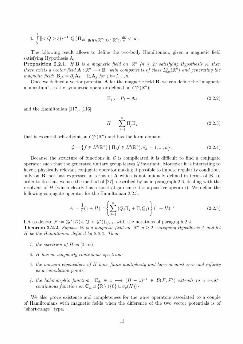
Let us denote F := (G∗;D(< Q >;G∗))1/2,1, with the notations of paragraph 2.4.Theorem 2.2.2. Suppose B is a magnetic field on Rn, n ≥ 2, satisfying Hypothesis A and letH be the Hamiltonian defined by 2.2.3. Then:

1. the spectrum of H is [0,∞);

2. H has no singularly continuous spectrum;

3. the nonzero eigenvalues of H have finite multiplicity and have at most zero and infinityas accumulation points;

4. the holomorphic function: C± 3 z 7−→ (H − z)−1 ∈ B(F ;F∗) extends to a weak∗-continuous function on C± ∪ R \ (0 ∪ σp(H)).

We also prove existence and completeness for the wave operators associated to a coupleof Hamiltonians with magnetic fields when the difference of the two vector potentials is of”short-range” type.

13

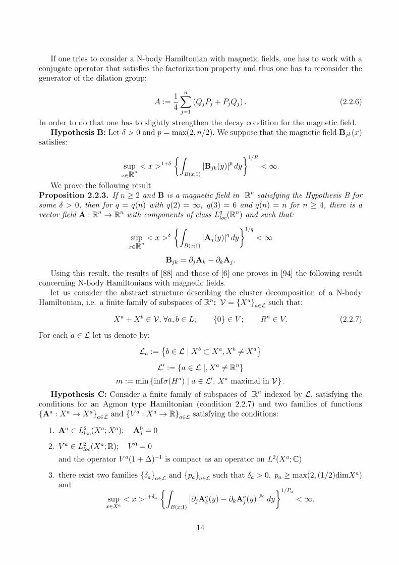
If one tries to consider a N-body Hamiltonian with magnetic fields, one has to work with aconjugate operator that satisfies the factorization property and thus one has to reconsider thegenerator of the dilation group:

A :=1

4

n∑j=1

(QjPj + PjQj) . (2.2.6)

In order to do that one has to slightly strengthen the decay condition for the magnetic field.Hypothesis B: Let δ > 0 and p = max(2, n/2). We suppose that the magnetic field Bjk(x)

satisfies:

supx∈Rn

< x >1+δ

∫B(x;1)

|Bjk(y)|p dy1/P

<∞.

We prove the following resultProposition 2.2.3. If n ≥ 2 and B is a magnetic field in Rn satisfying the Hypothesis B forsome δ > 0, then for q = q(n) with q(2) = ∞, q(3) = 6 and q(n) = n for n ≥ 4, there is avector field A : Rn → Rn with components of class Lqloc(R

n) and such that:

supx∈Rn

< x >δ

∫B(x;1)

|Aj(y)|q dy1/q

<∞

Bjk = ∂jAk − ∂kAj.

Using this result, the results of [88] and those of [6] one proves in [94] the following resultconcerning N-body Hamiltonians with magnetic fields.

let us consider the abstract structure describing the cluster decomposition of a N-bodyHamiltonian, i.e. a finite family of subspaces of Rn: V = Xaa∈L such that:

Xa +Xb ∈ V , ∀a, b ∈ L; 0 ∈ V ; Rn ∈ V. (2.2.7)

For each a ∈ L let us denote by:

La :=b ∈ L | Xb ⊂ Xa, Xb 6= Xa

L′ := a ∈ L |, Xa 6= Rn

m := min infσ(Ha) | a ∈ L′, Xa maximal in V .Hypothesis C: Consider a finite family of subspaces of Rn indexed by L, satisfying the

conditions for an Agmon type Hamiltonian (condition 2.2.7) and two families of functionsAa : Xa → Xaa∈L and V a : Xa → Ra∈L satisfying the conditions:

1. Aa ∈ L2loc(X

a;Xa); A0j = 0

2. V a ∈ L2loc(X

a;R); V 0 = 0

and the operator V a(1 + ∆)−1 is compact as an operator on L2(Xa;C)

3. there exist two families δaa∈L and paa∈L such that δa > 0, pa ≥ max(2, (1/2)dimXa)and

supx∈Xa

< x >1+δa

∫B(x;1)

∣∣∂jAak(y)− ∂kAa

j (y)∣∣pa dy1/Pa

<∞.

14

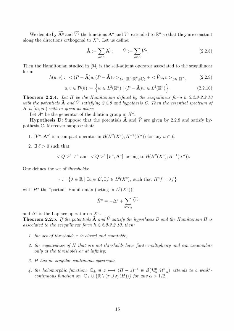
We denote by Aa and V a the functions Aa and V a extended to Rn so that they are constantalong the directions orthogonal to Xa. Let us define:

A :=∑a∈L

Aa; V :=∑a∈L

V a. (2.2.8)

Then the Hamiltonian studied in [94] is the self-adjoint operator associated to the sesquilinearform:

h(u, v) :=< (P − A)u, (P − A)v >L2( Rn

;Rn⊗C)

+ < V u, v >L2( Rn

)(2.2.9)

u, v ∈ D(h) :=w ∈ L2(Rn) | (P − A)w ∈ L2(Rn)

. (2.2.10)

Theorem 2.2.4. Let H be the Hamiltonian defined by the sesquilinear form h 2.2.9-2.2.10with the potentials A and V satisfying 2.2.8 and hypothesis C. Then the essential spectrum ofH is [m,∞) with m given as above.

Let Aa be the generator of the dilation group in Xa.Hypothesis D: Suppose that the potentials A and V are given by 2.2.8 and satisfy hy-

pothesis C. Moreover suppose that:

1. [V a,Aa] is a compact operator in B(H2(Xa);H−2(Xa)) for any a ∈ L

2. ∃ δ > 0 such that

< Q >δ V a and < Q >δ [V a,Aa] belong to B(H2(Xa);H−1(Xa)).

One defines the set of thresholds:

τ :=λ ∈ R | ∃a ∈ L′,∃f ∈ L2(Xa), such that Haf = λf

with Ha the ”partial” Hamiltonian (acting in L2(Xa)):

Ha = −∆a +∑b∈La

V b

and ∆a is the Laplace operator on Xa.Theorem 2.2.5. If the potentials A and V satisfy the hypothesis D and the Hamiltonian H isassociated to the sesquilinear form h 2.2.9-2.2.10, then:

1. the set of thresholds τ is closed and countable;

2. the eigenvalues of H that are not thresholds have finite multiplicity and can accumulateonly at the thresholds or at infinity;

3. H has no singular continuous spectrum;

4. the holomorphic function: C± 3 z 7−→ (H − z)−1 ∈ B(H0α,H0

−α) extends to a weak∗-continuous function on C± ∪ R \ (τ ∪ σp(H)) for any α > 1/2.

15

2.3 Obtaining Hardy type estimations from commutator estima-tions

Another direction of research that I have developed in collaboration with Marius Mantoiu,starting from the study of conjugate operators has been to obtain a class of weighted, HardyType estimations, starting from commutator estimations and to use this weighted estimationsin obtaining decay properties of eigenfunctions of some pseudodifferential operators. Theseresults are contained in [123, 124, 125, 130].

Let me present this type of results by using the text in the Introduction of [123].Given a self-adjoint operator H acting in L2(Rn) and a real number E one can consider the

problem of obtaining estimations of the type:

‖w1f‖ ≤ C ‖w2(H − E)f‖ (2.3.1)

for f in the domain of H and supported away from the origin and with w1 and w2 some givenweight functions. They allow one to deduce a given decay for f once that (H − E)f has aspecific decay. This kind of estimations already appeared in well-known papers as [1], [2], [42].Some of the works on this subject ([4], [5], [68], [69], [134], [143]) may indicate that one canprove such estimations using a special type of positivity condition associated with the existenceof a conjugate operator, an object very useful for the spectral analysis of the operator H. Moreprecisely, we say that H satisfies a Mourre estimation with respect to the conjugate operatorA, at a real value E, when (denoting by EJ(H) the spectral projection of H on an interval Jcontaining E) one has a strictly positive constant α such that:

iEJ(H)[H,A]ϕJ(H) ≥ αEJ(H). (2.3.2)

Let us outline our general argument leading from a Mourre estimation to a Hardy typeinequality (2.3.1) and use it for the special case H = λ(−i∇) with λ a sufficiently regularfunction defined on Rn (this choice is related to some applications to quantum Hamiltonians).

In proving (2.3.1), the position of the value E with respect to the spectrum of H playsan important role. For example, for simple differential operators, if E does not belong to thespectrum of the operator, then (2.3.1) reduces to an estimation on the resolvent of H andcan be proved by direct calculations involving the integral kernels. In this context we want toemphasize that the result we obtain is valid also for E belonging to the spectrum of H as longas it is in the complementary set of some critical values (see Definition 2.3.3); in the case of theLaplace operator for example, 0 is the only critical value. The idea of our method, as inspiredfrom the papers [5], [68], consists basically in reconsidering the proof of the main theorem in[2] starting not from a positivity condition but from a Mourre type estimation.

Let us first present the results obtained in [123] by using parts of this paper. Here are thedefinition of the framework and the precise statement of our main results. We work in Rn,with the Lebesgue measure denoted by dnx and with x · y, |x| denoting the Euclidean scalarproduct and norm. In order to simplify some formulae we denote the Fourier-Lebesgue measuredx:=(2π)−n/2dnx. We consider the Hilbert space

H := L2(Rn; dx) ≡L2(Rn)

and we denote by < f, g > and ‖f‖ the corresponding scalar product and norm. On L1(Rn; dx)we consider the Fourier transform:

F(f)(k) ≡ f(k) :=

∫Rne−ix·kf(x)dx (2.3.3)

16

and extend it to an isometry of L2(Rn). For the inverse Fourier transform we use the notations(F−1f)(x) ≡ f(x). We denote by δj the multiindex with 1 on position j ∈ 1, ...n and 0elsewhere. For a family of n commuting variables X := (X1, ..., Xn) we set:

Xα := Xα11 ...Xαn

n ; < X >:=

1 +

n∑j=1

X2j

1/2

. (2.3.4)

In H we shall work with the self-adjoint closures of:

(Qjf)(x) := xjf(x),∀f ∈ C∞0 ( Rn) (2.3.5)

Djf := −i ∂f∂xj

,∀f ∈ C∞0 (Rn). (2.3.6)

For a fixed y ∈ Rn we set y ·D :=∑n

j=1 yjDj.For any Borel function Φ : Rn → C we denote by Φ(Q), respectively by Φ(D) the operators

defined by the usual functional calculus for commuting families of self-adjoint operators and byD(Φ(Q)), respectively by D(Φ(D)) their domains in H.

Let BC(Rn) be the space of bounded, continuous functions on Rn and BC∞( Rn) thespace of indefinitely differentiable functions on Rn that are bounded together with all theirderivatives. S(Rn) will be the space of Schwarz functions on Rn with the usual local convextopology and S ′(Rn) its dual, the space of tempered distributions. We denote by: < ., . >:S ′(Rn) × S(Rn) → C the canonical antiduality (antilinear in the first factor and linear in thesecond one). This application restricts to the usual scalar product in L2(Rn) if one takes intoaccount the continuous inclusions: S(Rn) ⊂ L2(Rn) ⊂ S ′(Rn). For any function F ∈ L1

loc(Rn)we denote by the same letter its associated distribution. Sometimes we shall indicate by asubscript the variable in which a distribution acts. We set f−(x) := f(−x).

We shall mainly deal with analytic functions on a strip and we shall need some notations. LetCnδ := z ∈ Cn | |Imzj| < δ, j ∈ 1, ..., n and O(Cn

δ ) be the space of analytic functions in Cnδ .

Our intention is to study convolution operators with functions λ of class O(Cnδ ). Meanwhile, our

techniques involve the Fourier transform of λ and we have to ask it to be a bounded measure.For a finite complex measure ν on Rn let us denote by |ν| its total mass and by M( Rn)

the space of finite complex measures on Rn with the norm: ‖ν‖M := |ν| (Rn). FM(Rn) willbe the space of Borel functions on Rn that are Fourier transforms of measures in M(Rn).For a function µ ∈ FM( Rn) we denote by µ(dk) its Fourier transform with the convenientnormalization in order to have:

µ(x) =

∫Rneix·kµ(dk). (2.3.7)

Definition 2.3.1. Let O0(Cnδ ), be the set of analytic functions λ on the strip Cn

δ , such thatfor any y ∈ Rn with |yj| < δ the function Rn 3 x 7−→ λ(x+ iy) ∈ C is in FM( Rn).Proposition 2.3.2. If λ ∈ O0(Cn

δ ), let λy be the restriction of λ to the hyperplane Hy ≡ z ∈Cn | Imzj = yj. Then eγ|.|λ0 ∈M(Rn) for γ < δ.

Here is the main result of [123]. For simplicity of notation we shall systematically denoteby the same letter λ the restriction to Rn of the function λ ∈ O0(Cn

δ ).Definition 2.3.3. For a function λ ∈ O0(Cn

δ ) we define its set of regular values as

E(λ) :==t ∈ R | ∃ε > 0,∃κ > 0 s.t. |∇λ(k)| ≥ κ ∀k ∈ λ−1((t− ε, t+ ε))

.

We call generalized critical value a point in R \ E(λ).

17

Remark 2.3.4. It is obvious that E(λ) is open and that the image by λ of any zero of ∇λ isa generalized critical value. But λ may also have some other generalized critical values, due toits behaviour at infinity.Theorem 2.3.5. Let δ > 0, λ ∈ O0(Cn

δ ) and E ∈ E(λ). Then there is a strictly positiveconstant γ0 < δ such that for any γ ∈ (0, γ0) there is a positive constant C (depending on γand E) for which the following estimation holds for any f ∈ H:∥∥eγ<Q>f∥∥ ≤ C

∥∥∥√< Q >eγ<Q>(λ(D)− E)f∥∥∥ .

The inequality in the above statement is understood in the sense that if the function:

x 7−→√< x >eγ<x>((λ(D)− E)f)(x) (2.3.8)

is in L2( Rn) then the function eγ<x>f(x) is also in L2(Rn) and we have the stated estimation.Let us remark that in the above statement E may belong to the spectrum of the operator λ(D)as well as to its resolvent set as long as it remains a regular value.Theorem 2.3.6. Let λ and E be as in Theorem 2.3.5 and VI be the multiplication operatorwith a bounded function such that:

lim|x|→∞

< x > |VI(x)| = 0.

Let HI := H + VI , E be an eigenvalue of HI that belongs to E(λ) and g be an associatedeigenfunction. Then there exists a strictly positive constant γ such that eγ|x|g(x) is an L2(Rn)function.

In [130] we improve the above result of Theorem 2.3.5 by extending it to a class of convolutionoperators with Fourier transforms of polynomially growing functions analytic in a strip of theform |Imzj| < δ for j ∈ 1, ..., n. In fact most of the applications to the study of quantumHamiltonians, that one would like to consider, deal with this type of functions.

We consider convolution operators with functions λ of class O(Cnδ ) having a ”symbol-type”

behaviour for |Rezj| going to ∞. In order to cover analytic functions that grow at infinity inthe real directions we shall define the following function spaces.Notation 2.3.7. For any real s we define some function spaces:

Ss0(Rn) :=ρ ∈ C∞pol(Rn) |

|(∂αρ)(x)| ≤ Cα min< x >s−|α|, < ρ(x) >, ∀α ∈ Nn,

Os0(Cnδ ) := λ ∈ O(Cn

δ ) | λ(·+ iy) ∈ Ss0(Rn)

with uniform estimates for maxj|yj| < γ for any γ ∈ (0, δ).

We denote by G the domain of the self-adjoint operator λ(D) with the norm:

‖f‖2G := ‖f‖2 + ‖λ(D)f‖2 . (2.3.9)

We also setL := G ∩ L2

comp( Rn). (2.3.10)

Definition 2.3.8. For a function λ ∈ Os0(Cnδ ) we define its set of regular values:

E(λ) :=t ∈ R | ∃ε > 0,∃κ > 0 s.t. |∇λ(k)| ≥ κ ∀k ∈ λ−1((t− ε, t+ ε))

.

18

We call generalized critical value a point in the complementary set of E(λ) in R.Remark 2.3.9. It is obvious that E(λ) is open in R and that the image by λ of any point where∇λ = 0 is a generalized critical value; meanwhile it may happen that, due to its behaviour atinfinity, λ may also have some other generalized critical values.Theorem 2.3.10. Let δ > 0, λ ∈ Os0(Cn

δ ) and E ∈ E(λ). Then there is a strictly positiveconstant γ0 < δ such that for any γ ∈ (0, γ0) there is a positive constant C (depending on γand E) for which the following estimate holds for any f ∈ G:∥∥eγ<Q>f∥∥G ≤ C

∥∥∥√< Q >eγ<Q>(λ(D)− E)f∥∥∥ .

Remark 2.3.11.In the above statement E may belong to the spectrum of the operator λ(D)as well as to its resolvent set as long as it remains a regular value.Remark 2.3.12. The conclusion of Theorem 2.3.10 remains true if one replaces the operatorλ(D) by λ(D)+V for any real function V defined on Rn that is relatively bounded with respectto λ(D) and satisfies the decay condition:

limR→∞‖χ(|Q| > R) < Q > V (Q)(λ(D) + i)−1‖ = 0

From this result, by the argument in [123], one can deduce an a-priori decay estimate foreigenfunctions of λ(D) + V , associated to eigenvalues E ∈ E(λ).Remark 2.3.13. In fact one can prove a slightly more general form of our Theorem 2.3.10for functions of the form λ = µρ with µ analytic and being the Fourier transform of a finitemeasure and ρ ∈ Os0(Cn

δ ); this proof is a straightforward mixture of the arguments in [123] andthose of [130] but involve rather cumbersome formulae.Remark 2.3.14. The functions λ that we consider are not supposed to be polynomials (i.e.their Fourier transforms need not be supported in 0) and this is responsible for most of thecomplications we encounter. Let us mention in this direction that the only case of this typeappearing in the literature is the particular case λ(x) = (1 + |x|2)1/2 ([43], [78]).Remark 2.3.15. A rather obvious modification of our Theorem 2.3.6 allows to extend theresult of Theorem 2.3.10 to perturbations of “short range type” (with differential operatorswith nonconstant coefficients) obtaining a generalization of Theorem 14.5.2 in [85] for nonlocalconvolution operators and exponential weights. Moreover, by repeating the arguments in ourproof of Theorem 2.3.10 for an operator of the form λ(D)+V (Q,D) with V of “long range type”one could extend Theorem 30.2.9 in [87] for nonlocal convolution operators and exponentialweights.

2.3.1 Decay of eigenfunctions of perturbed periodic Hamiltonians

In [124] we consider the problem of using the above ideas for obtaining upper bounds for therate of decay at infinity for eigenfunctions of perturbed periodic Schrodinger operators. Moreprecisely, let us fix a Hamiltonian of the form HI := H + VI where H := −∆ + V is a periodicSchrodinger operator in dimension n and VI is a perturbation decaying at infinity (faster then|x|−1). We shall suppose that the spectrum of H has an isolated part at the bottom that can bedescribed by N analytic eigenvalues with analytic associated eigenprojectors (for example if thefirst band is isolated), more precisely we shall impose our Hypothesis 2.3.16 below. Under theseconditions we show that any eigenvalue of the perturbed Hamiltonian HI that is a regular value(more precisely see Definition 2.3.17), has eigenfunctions that decay exponentially at infinity,

19

with an exponent linear in |x| (see Theorem 2.3.19). Let us remark that our result covers alsothe case of embedded eigenvalues as long as they are regular.

Let us point out that the existence of embedded eigenvalues for perturbations of periodicSchrodinger operators has been subject to intensive work. In [119] it is shown that for anycontinuous V and any number E belonging to the spectrum of H, there exists a function VIwhich is O(< x >−1) at infinity such that E is an eigenvalue of H + VI . In more than onedimension the situation is less clear. Anyway, if n = 2 or 3, for some classes of periodic V ’s,eigenvalues embedded into the spectrum of H are forbidden if one imposes the very restrictivecondition

|VI(x)| ≤ Cexp(−|x|4/3+ε)

for a strictly positive ε (see [105]).We obtain our result (Theorem 2.3.19) by using our ideas and results presented above

and by first proving a weighted estimation of Hardy type (with exponential weights) for theunperturbed periodic HamiltonianH (Theorem 2.3.18). In our case we shall isolate the boundedenergy region of the first N bands for which we shall apply a generalization of our previousmethod and the rest of the spectrum for which we shall use a variant of the general method ofAgmon [2].

We shall denote by ∇ and ∆ the usual gradient and Laplace operators on C∞0 (Rn) and byH2(Rn) the Sobolev space of second order. Let p = 2 for n=1,2,3, p > n/2 for n ≥ 4 and letV ∈ Lploc(Rn;R) be Zn-periodic on Rn. By some obvious modifications one can also consider ageneral type of lattice. We consider the Hamiltonian:

H = −∆ + V (2.3.11)

to be the usual self-adjoint operator in L2(Rn) (having domain H2(Rn), see [152]). The well-known Floquet representation allows one to decompose H as a direct integral corresponding tothe representation: L2(Rn) ∼= L2(Tn;L2(Ω)) , where:

Tn := Rn/Zn ∼= (S1)n; Ω := [0, 1)n (2.3.12)

are the n-dimensional torus and the fundamental domain associated to Zn. In the following weidentify functions defined on Tn with periodic functions on Rn.

The Hamiltonian H is decomposable with respect to the above representation and each”fibre Hamiltonian” H(τ) (for τ ∈ Tn) has compact resolvent and thus a discrete spectrumλa(τ)a∈N, defining the so-called ”band functions”. Due to the fact that our procedure relieson the regularity of the functions: Tn 3 τ 7−→ λa(τ) and being well known that for n > 1 somedifficult problems appear in this context, we are obliged to impose some implicit conditionsthat we now formulate.

We shall denote by:

P(L2(Ω)) :=P ∈ B(L2(Ω)) | P 2 = P = P ∗

. (2.3.13)

Hypothesis 2.3.16. By denoting σ(H) the spectrum of the operator H, we assume:a) σ(H) = σ0 ∪ σ∞, where: (inf σ∞)− (supσ0) = d0 > 0;b) there is some N ∈ N∗ and for each a ∈ 1, ..., N two functions:

λa : Tn → R , πa : Tn → P(L2(Ω)) (2.3.14)

20

that are analytic (with respect to the uniform topology on P(L2(Ω)) in the second case) and admitholomorphic extensions to some strip Cn

δ for some δ > 0, such that the Hamiltonian H reducedto the spectral subspace associated to σ0 is unitarily equivalent, in the Floquet representation,to multiplication with the following operator-valued function of τ ∈ Tn:

N∑a=1

λa(τ)πa(τ). (2.3.15)

Let us remark that our Hypothesis covers the usual case in which the spectrum of H has anisolated band at its bottom, but also the situation of several bands, even overlapping, as longas one can assure the analyticity of the eigenvalues and of the eigenprojections.Definition 2.3.17. Let us denote by E0(H), the set of points t < inf σ∞ such that ∃ε >0, ∃α0 > 0 for which |(∇λa)(τ)| ≥ α0, ∀τ ∈ λ−1

a ((t− ε, t+ ε)) and ∀a ∈ 1, ..., N. We call thisset, the regular set of H below σ∞.

Let us remark that E0(H) is the complement in (−∞, inf σ∞) of the set of critical valuesof the functions λ1, ..., λN. With these notations we can state now the main results of ourwork, that will be proved in Section 3.Theorem 2.3.18. Let H be a periodic Schrodinger Hamiltonian satisfying the Hypothesis 2.3.16and let E ∈ E0(H). Then there exists a constant κ0 ∈ (0, 2πδ) such that for any κ ∈ (0, κ0)there exists a positive constant C (depending on E and κ) for which:∥∥eκ<Q>f∥∥D(H)

≤ C∥∥∥√< Q >eκ<Q>(H − E)f

∥∥∥ , ∀f ∈ D(H). (2.3.16)

We have denoted by ‖.‖D(H) the graph norm with respect to H.Theorem 2.3.19. Let H be a periodic Schrodinger operator (2.3.11) for which Hypothesis2.3.16 stands true. Let VI be a potential of class Lploc(Rn) (with p as defined before (2.3.11)),such that lim

|x|→∞< x > |VI(x)| = 0. Then for any eigenvalue E of the Hamiltonian HI := H+VI

that belongs to E0(H) there exists κ ∈ (0, δ) such that for any corresponding eigenvector g:

eκ<Q>g ∈ L2(Rn). (2.3.17)

3 Propagation properties for the Dirac operator

A second research direction, suggested by Gheorghe Nenciu, started from a problem left open inthe study presented in [141]: the completeness of the wave operators for a Dirac Hamiltonianwith a time dependent potential defined as the solution of the free Maxwell equations withregular and compactly supported initial data. This problem is of interest in connection withthe study of the Dirac Quantum Field in interaction with an external electromagnetic field.It can be shown [T] that if the ”one-particle ” scattering matrix exists and satisfies a specialproperty, then the scattering matrix for the quantum field also exists and can be computed bythe second quantization procedure. This problem is considered in [P] but only partial results areobtained and nothing is said concerning the completeness of the ”one-particle” wave operators.In [33] we restrict ourselves to the case of compactly supported electromagnetic fields and provethat the wave operators exist and are unitary.

We work in the Hilbert space H := L2(R3) ⊗ C4 and we shall denote by Qj the operatorof multiplication with xj in H and by Dj the operator −i∂/∂xj = −i∂j. We shall also use the

21

notations: D := −i∇, ∂t := ∂/∂t. We shall denote by < ξ >:= 1 + |ξ|21/2for ξ ∈ Rn and also

for n-tuples of commuting selfadjoint operators by using the functional calculus for selfadjointoperators. We shall denote by B(x0, R) the closed ball of radius R and center x0 and byS(x0, R) its surface. For any subset M in Rn we shall denote by χM its characteristic functionand by M c its complementary in Rn. Moreover we shall denote by χ(|Q| < R) the self-adjointoperator associated to the function χ|ξ|<R, by the functional calculus for selfadjoint operatorsand similarly for ”<” replaced by ”≤, >,≥”. We denote by B(H) the algebra of bounded linearoperators on H and by B(C4) the algebra of linear operators on C4. For any s ∈ R we denoteby Hs(R3) the Sobolev space of order s on R3 with the norm: ‖u‖s := ‖ < D >s u‖L2(R3) andHs := Hs(R3)⊗ C4. Let us consider a Dirac Hamiltonian describing an electron in interactionwith an external electromagnetic field without sources. We shall consider the light velocityc = l. The electromagnetic field in the Coulomb gauge is described by a three component realvector field Aj(x, t) with j ∈ 1, 2, 3 and x ∈ R3, t ∈ R that satisfies the homogeneous waveequation : (

∂2

∂t2−∆

)Aj = 0, for j = 1, 2, 3. (3.0.1)

We consider the following type of initial data:Aj(x, 0) := aj(x), with aj ∈ C∞0 (R3)(∂tAj

)(x, 0) := bj(x), with bj ∈ C∞0 (R3).

(3.0.2)

⋃j=1,2,3

(supp aj ∪ suppbj) ⊂ B(0, R). (3.0.3)

It is well-known that the solution of (3.0.1) in R3 can be written in the form :

Aj(x, t) =1

4π

∂

∂t

(t

∫|y|=1

aj(x+ ty) dσ(y)

)+ t

∫|y|=1

bj(x+ ty) dσ(y)

. (3.0.4)

Let αj for j = 1, 2, 3 and β be the Dirac matrices (complex hermitian 4 by 4 matrices) sothat the Dirac Hamiltonian will be :

H(t) = −iα · ∇ + mβ + eα · A = H0 + V (t)H0 = −iα · ∇ + mβV (t) = eα · A

(3.0.5)

where m > 0. Sometimes we shall denote the unit matrix in C4 by α0 in order to simplify somenotations. We shall be interested in the nonhomogeneous time evolution on H generated bythe family H(t)t∈R given by (3.0.5) i.e. the two parameter family U(t, s)(t,s)∈R2 of unitaryoperators on H, solution of the Cauchy problem :

i∂tU(t, s) = H(t)U(t, s)U(s, s) = 1l.

(3.0.6)

One can easily observe that for |t| → ∞, H(t) goes in norm resolvent sense to H0 and we wouldlike to compare the nonhomogeneous evolution U(t, s) with the free one generated by H0, i.e.U0(t, s) = exp−itH0. We shall define the operators:

Ws(t) := U(s, t)U0(t− s), W ∗s (T ) = U0(s− t)U(t, s). (3.0.7)

22

and we shall study the existence of their limits when |t| → ∞, with respect to the strongoperator topology on B(H). Our main result is that for t → ±∞ both the above operatorshave limits in the strong topology. We denote these limits by: W±

s and (W±s )∗ for any s ∈ R.

First we obtain some propagation estimations for the free evolution U0. Let us introducethe following notations. For k ∈ R3 we shall denote by v(k) ∈ R3 the classical velocity

corresponding to the momentum k, for the free movement, i.e. v(k) =(√|k|2 +m2

)−1k and

for K ∈ R+ we denote by u(K) := K(√

K2 +m2)−1

.

Proposition 3.0.1. Let f ∈ H be such that its Fourier transform satisfies f ∈ C∞0 (R3) ⊗ C4

with suppf ⊂ B(0, K), then for any N ∈ N there is some CN < ∞, depending on N and f ,such that for t > 0 one has:∥∥χ(|Q| ≥ u(2K)t

)U0(t)

∥∥ ≤ CN(1 + t)N

.

Proposition 3.0.2. Let f ∈ H such that f ∈ C∞0 (R3) ⊗ C4 with suppf ∈ B(0, r), then fort ∈ R+, u0 ∈ (0, 1) and x ∈ R3 with |x| > r+ ut and u ∈ [u0, l) we have that for any N ∈ N wecan find a constant CN <∞ depending only on N and u0 but not on f , such that:∣∣(U0(t)f

)(x)∣∣ ≤ CN t

(1− u2

)N/2 ∥∥∥(1l−∆)(N+2)/2

f∥∥∥L2(R3

.

Using the asymptotic properties of the solutions of the free Maxwell equations we obtainsome propagation estimations for the perturbed, time-dependent, evolution.Proposition 3.0.3. For any f in the domain of the self-adjoint operator < Q > we have thefollowing estimation:

‖QjU(t, s)f‖ ≤ C ‖Qjf‖ + |t− s|‖f‖ .

Proposition 3.0.4. For any l ∈ N, if f ∈ Hl, we have the estimation:∥∥|D|lU(t, s)∥∥ ≤ C

‖|D|lf‖ +

(ln(1 + |t− s|)

)l‖f‖ .An important tool is the use of energetic inequalities in the same way as Chernoff [45] in

order to derive some propagation properties in the regions where there is no field. We shallstart with reviewing the inequality proven by Chernoff. We shall denote the scalar product inC4 by < ·, · >.Proposition 3.0.5. Let f ∈ H and let us denote by f(t, x) :=

(U(t, s)f

)(x). Then, for any

t ∈ R+, with t ≥ s, we have the estimation:∫B(x0,r)

〈f(t, x), f(t, x)〉d3x =

∫B(x0,r+t−s)

〈f(s, x), f(s, x)〉d3x.

Using these propagation estimations, we prove the following result.Theorem 3.0.6. The operators W±

0 exist and are unitary in H.In [35] we extend this result from the compactly supported smooth initial data for the

electromagnetic field to the case of initial data rapidly decaying in space.Related to this research direction is also our paper [34] in which we generalize the results of

[45] to the case of perturbations that do not preserve the operator domain and can be definedonly in the sense of sums of quadratic forms. For that we use a slightly different technique that

23

does not make use of the Kato-Trotter formula, and thus can be applied to our situation wherethe sum is defined only in the form-sense. We consider operators of the form H = H0 +V withH0 given as in (3.0.5) and

V : R3 → Bh(H) := A ∈ B(H) | A∗ = A . (3.0.8)

We shall consider three different hypotheses that V can satisfy.

Hypothesis H1 For any ϕ ∈ C∞0 (R3;R) we have ϕV ∈ B(H1/2;H−1/2

), so H0 + ϕV can be

defined as a sum of operators in B(H1/2;H−1/2

).

Hypothesis H2 For any ϕ ∈ C∞0 (R3;R) the operator Hϕ := H0 + ϕV defined on

Dϕ :=f ∈ H1/2 | Hϕf ∈ H

is a self-adjoint operator.

Hypothesis H3 The self-adjoint operator H, defined in hypothesis H2, is well defined andessentially self-adjoint on C∞0

(R3;C4

).

Theorem 3.0.7. Suppose H0 is given as in (3.0.5) and V : R3 → Bh(H) satisfies the HypothesisH1 and H2. Then there exists a unique self-adjoint operator H in H such that:

1. D(H) ⊂ H1/2loc ;

2. ∀f ∈ D(H), ∀g ∈ H1/2c , we have the equality

(Hf, g

)=(f,H0g

)+(f, V g

).

If the Hypothesis H1- H3 are satisfied, then H is essentially self-adjoint on C∞0(R3;C4

).

4 Mathematical description of quantum systems in mag-

netic fields

This section describes the research direction that has somehow followed my activity over theyears, revealing a diversity of aspects and problems that I continue to study and hopefullyto gather as a monography dedicated to the mathematical description of the quantum ”mag-netic dynamical systems’. I shall begin by presenting some material from [129] concerning the’classical’ dynamical systems in magnetic fields.

4.1 The classical particle in a magnetic field

In this section we shall give a classical background for our quantum formalism. We use thesetting and ideas in [120] but develop the gauge invariant Poisson algebra feature. We begin byvery briefly recalling the usual Hamiltonian formalism for classical motion in a magnetic fieldand then change the point of view by perturbing the canonical symplectic structure. We useprinted material from [129].

24

4.1.1 Two Hamiltonian formalisms.

The basic fact provided by physical measurements is that the magnetic field in R3 may bedescribed by a function B : R3 → R3 with divB = 0, such that the motion R 3 t 7→ q(t) ∈ R3

of a classical particle (mass m and electric charge e) is given by the equation of motion definedby the Lorentz force:

mq(t) = eq(t)×B(q(t)) (4.1.1)

where × is the antisymmetric vector product in R3 and the upper point denotes derivation withrespect to time. An important fact about this equation of motion is that it can be derived froma Hamilton function, the price to pay being the necessity of a vector potential, i.e. a vectorfield A : R3 → R3 such that B = rotA, that is unfortunately not uniquely determined (thegauge group of symmetries for the theory).

Let us very briefly recall the essential facts concerning the Hamiltonian formalism. Given asmooth manifold X we associate to it its “phase space” defined as the cotangent bundle T∗X onwhich we have a canonical symplectic form, that we shall denote by σ. If we set Π : T[T∗X]→T∗X and π : T∗X → X the canonical projections and π∗ : T[T∗X] → TX the tangent map ofπ, then σ := dβ where β(ξ) := [Π(ξ](π∗(ξ)), for ξ a smooth section in T[T∗X]. A Hamiltoniansystem is determined by a Hamilton function h : T∗X → R (supposed to be smooth) such thatthe vector field associated to the law of motion of the system (R 3 t 7→ x(t) ∈ T∗X) is given bythe following first order differential equation ξyσ − dh = 0, where ξyσ is the one-form definedby (ξyσ)(η) := σ(ξ,η), for any η smooth section in T[T∗X].

Let us take X = R3 such that all the above bundles are trivial and we have canonicalisomorphisms T∗X ∼= X × X∗ (that we shall also denote by Ξ) and T[T∗X] ∼= (X × X∗) ×(X × X∗), defined by the usual transitive action of translations on X; we can view any twosections ξ and η as functions ξ(q, p) = (x(q, p), k(q, p)), η(q, p) = (y(q, p), l(q, p)) and we caneasily verify that σ(ξ,η) = k · y− l ·x, with ξ · y the canonical pairing X∗×X → R. Moreover,the equations of motion defined by a Hamilton function h become:

qj = ∂h/∂pj,pj = −∂h/∂qj.

(4.1.2)

Then (4.1.1) may be written in the above form if one chooses a vector potential A such thatB = rotA and defines the Hamilton function

hA(q, p) := (2m)−1

3∑j=1

(pj − eAj(q))2.

Although very useful, this Hamiltonian description has the drawback of involving the choice ofa vector potential. Two different choices A and A′ have to satisfy rot(A−A′) = 0. Since R3 issimply connected, there exists a function ϕ : R3 → R with A′ = A+∇ϕ and any such choice isadmissible. We call these changes of descriptions “gauge transformations”; the “gauge group”is evidently C∞(X) and the action of the gauge group is given by hA → hA′ .

An interesting fact is that we can actually obtain an explicitly gauge invariant descriptionby using a perturbed symplectic form on T∗X [61]. For that it is important to notice that themagnetic field may in fact be described as a 2-form (a field of antisymmetric bilinear functionson R3), due to the obvious isomorphism between R3 and the space of antisymmetric matriceson R3 (just take Bjk := εjklBl with εjkl the completely antisymmetric tensor of rank 3 on R3).Thus from now on we shall consider the magnetic field B given by a smooth section of the vector

25

bundle Λ2X → X (the fibre at x being T∗xX ∧ T∗xX ∼= [TxX ∧ TxX]∗). Due to the canonicalglobal trivialisation discussed above (defined by translations) we can view B as a smooth mapB : X → X∗ ∧X∗ ∼= (X ∧X)∗. Then a vector potential is described by a 1-form A : X → X∗

such that B = dA where d is the exterior differential. This also allows us to consider the caseX = RN for any natural number N .

Any k-form on X may be considered as a k-form on T∗X. Explicitly, using the projectionπ : T∗X → X, we may canonically define the pull-back π∗B of B and the “perturbed symplecticform” on T∗X defined by the magnetic field B as σB := σ + eπ∗B.

Now let us briefly recall the construction of the Poisson algebra associated to a symplecticform. We start from the trivial fact that any nondegenerate bilinear form Σ on the vector spaceΞ defines a canonical isomorphism iΣ : Ξ → Ξ∗ by the equality [iΣ(x)](y) := Σ(x, y). Thenwe define the following composition law on C∞(X): f, gB := σB(i−1

σB(df), i−1

σB(dg)), called the

Poisson braket. The case B = 0 gives evidently the canonical Poisson braket ., . on thecotangent bundle. A computation gives immediately

f, gB =N∑j=1

(∂pjf ∂qjg − ∂qjf ∂pjg

)+ e

N∑j,k=1

Bjk(·) ∂pjf ∂pkg. (4.1.3)

For the usual Hamilton function of the free classical particle h(p) := (2m)−1N∑j=1

p2j , we can

write down the Poisson form of the equation of motion:qj = h, qjB = 1

mpj,

pj = −h, pjB = em

N∑k=1

Bkj(q)pk,(4.1.4)

that combine to the equation of motion (4.1.1) defined by the Lorentz force.We remark finally that in the present formulation the Hamilton function of the free particle

h(q, p) = (2m)−1∑p2j is no longer privileged; any Hamilton function is now a candidate for

a Hamiltonian system in a magnetic field just by considering it on the phase space endowedwith the magnetic symplectic form. The relativistic kinetic energy h(p) := (p2 + m2)1/2 is aphysically interesting example.

Remark. The real linear space C∞(Ξ;R) endowed with the usual product of functions andthe magnetic Poisson braket ., .B form a Poisson algebra (see [127], [107]), i.e. (C∞(Ξ;R), ·)is a real abelian algebra and ., .B : C∞(Ξ;R) × C∞(Ξ;R) → C∞(Ξ;R) is an antisymmetricbilinear composition law that satisfies the Jacobi identity and is a derivation with respect tothe usual product.

4.1.2 Magnetic translations.

For the perturbed symplectic form on T∗X, the usual translations are no longer symplectic.We intend to define “magnetic symplectic translations” and compute the associated momentummap. Using the canonical global trivialisation, we are thus looking for an action X 3 x 7→ αx ∈Diff(X ×X∗) having the form αx(q, p) = (q + x, p + τx(q, p)). A group action clearly imposesthe 1-cocycle condition: τx+y(q, p) = τx(q, p) + τy(q + x, p+ τx(q, p)). The symplectic conditionreads: (α−x)

∗σB = σB. A simple computation gives us for any (q, p) ∈ Ξ:

[α−x]∗ =

(1 0

[τ−x]∗X 1 + [τ−x]

∗X∗

)∧2

: Λ2(q,p)(Ξ)→ Λ2

(q+x,p+τx(q,p))(Ξ), (4.1.1)

26

where we identified all the cotangent fibres

T∗(q,p)Ξ ∼= T∗qX ⊕ T∗p(T∗qX) ∼= T∗qX ⊕ T∗pX∗ (4.1.2)

[τ−x]∗X : T∗X∗ → T∗X, [τ−x]

∗X∗ : T∗X∗ → T∗X∗. (4.1.3)

Finally we obtain:[α−x]∗ σB − σB|(q+x,p+τx(q,p)) = (4.1.4)

N∑j,k=1

[T−x(q, p)]jkdqj ∧ dqk + [S−x(q, p)]jkdqj ∧ dpk ,

with (T x(q, p))jk =

= (∂/∂qj)(τx(q, p))k − (∂/∂qk)(τx(q, p))j + eB(q)jk − eB(q + x)jk, (4.1.5)

(Sx(q, p))jk = (∂/∂pj)(τx(q, p))k. (4.1.6)

Asking for αx to be symplectic implies that S = 0, hence τx does not depend on p. If we fixa point q0 ∈ X we can define the function a(x) := τx(q0) ∈ X∗ and the condition imposed onτx(q) for having a group action leads to τx(q + q0) = a(x + q) − a(q). Choosing q0 = 0 and avector potential A for B, the first equation in (4.1.5) implies (τx(q)) := eA(q + x)− eA(q).

Let us compute the associate differential action. We set [(DA(q)) · x]j :=∑

k[∂kAj(q)]xkand for x ∈ X we define the vector field in T(X ×X∗):

tx(q, p) := (∂/∂t) |t=0 α−tx(q, p) = (4.1.7)

= (−x, (∂/∂t) |t=0 τ−tx(q)) = (−x, e(DA(q)) · x).

Let us find the associated momentum map. A computation using the definition above (see also[127]) gives: [iσB ](x, l) = (l + exyB,−x), where (xyB)(y) := B(x, y). Then we obtain

[iσB ](tBx )(q,p) = (e(DA(q)) · x− exyB, x)(q,p) = (−d(eA(q) · x), x)(q,p),

with A(q)·x =N∑j=1

Aj(q)xj. It follows then that [iσB ](tBx ) = dγAx , where γAx (q, p) := x·p−eA(q)·x

and thus for any direction ν ∈ X (|ν| = 1) we have defined the infinitesimal observable magneticmomentum along ν to be γAν (q, p) := ν · (p− eA(q)). The momentum map ([120]) is thus givenby

µA : T∗X → X∗, [µA(q, p)](x) := γAx (q, p), (4.1.8)

i.e. µA(q, p) = p− eA(q).

4.1.3 Quantizing Hamiltonian systems in magnetic fields. The standard procedure

We insert here the presentation we did in [127].General principles assert essentially that classical observables are functions in phase space,

while quantum observables should be self-adjoint operators in some Hilbert space. Ratheroften, for some basic observables (positions, momenta,...) the prescription is either essentiallyunique (may be due to some commutation relations), or at least generally accepted. Thus, formany physical systems, quantization of all phase-space functions could be regarded as a sortof functional calculus. But since, due to the Heisenberg principle, the basic observables do

27

not commute, one cannot rely on the usual spectral theory to define this functional calculus.Roughly, quantization may be seen as the mathematical problem of defining functions of severalnon-commuting self-adjoint operators. Of course, the features of the physical system bothimpose constrains and offer empirical suggestions with respect to this procedure.

In the absence of any magnetic field, a non-relativistic spinless particle moving in RN isquantized through the Weyl pseudodifferential calculus. If f is a suitable function (“symbol”)defined on the phase space R2N , the corresponding operator is defined to act in the Hilbertspace L2(RN) by the formula

[Op(f)u](x) :=

∫R2N

dy dp ei(x−y)·pf

(x+ y

2, p

)u(y). (4.1.1)

In a certain sense (which can be made precise and which will be discussed below), we maywrite Op(f) = f(Q,P ) and interpret it as the action on the symbol f of the functional calculusassociated to the family of operators (Q1, . . . , QN , P1, . . . , PN), where Qj is the multiplicationby the j’th coordinate and Pj := −i∂j. The well-known rules of commutation between theseposition and momentum quantum observables play a decisive role in determining the explicitformula above. They are thus also basic in deducing the explicit product rule (f, g) 7→ f gand involution f 7→ f leading to Op(f)Op(g) = Op(f g) and Op(f)∗ = Op(f ).

When a magnetic field B is turned on, we are faced with the problem of modifying theformula for Op(f) in a way taking into account the presence of the magnetic field in a correct,physical way. A mistaken procedure which appears from time to time in the literature is thefollowing: One chooses a vector potential A corresponding to the magnetic field (B = dA)and, by an (unjustified) application of the minimal coupling principle, one sets OpA(f) :=Op(fA), with fA(x, p) := f(x, p−A(x)). This is meant to be the action on f of the functionalcalculus associated with the family Q1, . . . , QN ,Π1, . . . ,ΠN , where Πj := Pj−Aj(Q) is the j’thcomponent of the vector potential. But the resulting formula

[OpA(f)u](x) :=

∫R2N

dy dk ei(x−y)·kf

(x+ y

2, k − A

(x+ y

2

))u(y) = (4.1.2)

=

∫R2N

dy dp ei(x−y)·pei(x−y)·A(x+y2 )f

(x+ y

2, p

)u(y) (4.1.3)

cannot be the right one, since it lacks gauge covariance: If one chooses another vector potentialA′ associated to B, differing from the initial one by the gradient of a scalar function, A′ =A+∇ρ, then the expected formula eiρOpA(f)e−iρ = OpA′(f) does not hold.

In order to introduce our proposal for magnetic quantization let us come back to (4.1.1) andtry to understand it better. The Weyl ’functional calculus’ we mentioned there is describedon the Hilbert space H = L2(X) in terms of the family of self-adjoint operators (Qj)j=1,...,N

and (Pj)j=1,...,N (here Qj is the operator of multiplication with the j-th component of thevariable in H and Pj := −i∂j). The operators (Qj, Pj)j=1,...,N are the quantum version of theclassical observables position and momenta, given by the the canonical variables in phase spaceq1, · · · , qN , p1, . . . , pN . These canonical variables satisfy the relations

qi, qj = 0, pi, pj = 0, pi, qj = δij, i, j = 1, . . . , N.

28

The Weyl system In principle, the choice of the Hilbert space L2(X) and of the explicitform of the operators Qj and Pj should be justified. It is widely accepted the vague prescriptionthat to the canonical variables qj and pj one should ascribe self-adjoint operators Op(qj) andOp(pj) acting in some Hilbert space H, satisfying

i[Op(qi),Op(qj)] = 0, i[Op(pi),Op(pj)] = 0, i[Op(pi),Op(qj)] = δij, i, j = 1, . . . , N. (4.1.4)

But an axiomatic approach relying on this formulae is hard to conceive. The typical difficultiesrelated to the (inevitable) non-boundedness of the operators Op(qj) and Op(pj) cannot besolved by a priori arguments.

For this and for several other reasons, it is preferable to rephrase all in term of boundedoperators. For q ∈ X and p ∈ X?, let us set U(q) := e−iq·P and V (p) := e−iQ·p. These areunitary operators in L2(X) given explicitly by

[U(q)u](y) = u(y − q) and [V (p)u](y) = e−iy·pu(y), u ∈ L2(X), y ∈ X. (4.1.5)

The maps q 7→ U(q) and p 7→ V (p) are strongly continuous unitary representations of X,respectively X∗, in L2(X) and the Weyl form of the canonical commutation relations

U(q)V (p) = eiq·p V (p)U(q), q ∈ X, p ∈ X? (4.1.6)

holds. Now there is no ambiguity in addressing the abstract problem of the classification oftriples (H, U, V ), where H is a Hilbert space and U : X → U(H), V : X? → U(H) are stronglycontinuous unitary representations satisfying (4.1.6). And there is a simple answer, given bythe Stone-von Neumann Theorem (for a more explicit statement and for the proof we send to[70]): If one also assumes irreducibility of the family U(q), V (p) | q ∈ X, p ∈ X?, then anysolution is unitarily equivalent to (4.1.5) (which is called the Schrodinger representation). Anda non-irreducible triple is just a multiple of this Schrodinger representation.

A convenient way to condense the two objects U and V into a single one is to define theWeyl system W (X) | X ∈ Ξ ⊂ U(H) by

W (q, p) := ei2q·p U(−q)V (p) = e−

i2q·p V (p)U(−q), q ∈ X, p ∈ X?. (4.1.7)

A short calculation shows that W satisfies

W (ξ)W (η) = ei2σ(ξ,η) W (ξ + η), ξ, η ∈ Ξ, (4.1.8)

i.e. W is a projective representation of the group Ξ with 2-cocycle (phase factor) ei2σ.

Of course, W can be defined for any abstract triple (H, U, V ). But, as a consequence of theStone-von Neumann Theorem, it is enough to work with the Schrodinger representation. Thecorresponding W will be called the Schrodinger Weyl system and is explicitly given on L2(X)by

[W (q, p)u](y) = e−i(12q+y)·p u(y + q). (4.1.9)

The representations U and V can be recovered easily from W by U(q) = W (−q, 0) and V (p) =W (0, p). One easily justifies the formula W (ξ) = e−iσ(ξ,R), where R = (Q,P ); σ(ξ, R) signifieshere the (suitable defined) self-adjoint operator Q · p− q · P .

The Weyl system is a convenient way to codify the commutation relations between the basicoperators Q and P . In the next paragraph, the quantization by pseudodifferential operatorswill be obtained as an integrated form of this Weyl system.

29

Pseudodifferential operators If a family of self-adjoint operators S1, . . . , Sm is given suchthat for any i, j, Si and Sj commute, then one can define a functional calculus for this familyby one of the two formulae

f(S) =

∫Rm

f(λ)dES(λ) =

∫Rm

dt f(t)e−it·S.

Here ES is the spectral measure (on Rm) of the family S1, . . . , Sm, under suitable assumptionst · S := t1S1 + · · · + tmSm is a well-defined self-adjoint operator and f is the inverse Fouriertransform of f , conveniently normalized.

If, once again, S1, . . . , Sm are self-adjoint, but they no longer commute, there is usually noreasonable spectral measure ES. One can try to use the operator version of the Fourier inversionformula to define a functional calculus. The key point would be the ability of defining a suitableanalogue of e−it·S. This strategy is outlined in [8] (see also [9]) for very general situations. Butthe properties of the resulting functional calculus are quite modest if the commutation relationsof the operators Sj have no interesting peculiarities.

We have proposed such a program for Sj = Qj if j = 1, . . . , N and Sj = ΠAj for j =

N+1, . . . , 2N , with ΠAj = Pj−Aj(Q) the j’th component of the magnetic momentum defined by

a vector potential A. But we stop for a moment to fix some conventions on Fourier transforms.Let us start with two arbitrary Haar measures dx on X and dp on X∗. One defines at the levelof tempered distributions

FX ,FX : S ′(X)→ S ′(X∗), FX? ,FX? : S ′(X?)→ S ′(X),

uniquely determined by the following actions on integrable functions:

(FXu)(p) =

∫X

dx e−ix·pu(x), (FXu)(p) =

∫X

dx eix·pu(x),

(FX?v)(x) =

∫X?

dp e−ix·pv(p), (FX?v)(p) =

∫X?

dp eix·pv(p).

It is easily shown that there exists c > 0 such that

FX∗ FX = c idS′(X) and FX FX? = c idS′(X?).

Thus, by redefining dx and dp, one gets F−1X = FX? and F−1

X? = FX . We fix such a choicefor dx and dp, but obviously dξ := dx ⊗ dp does not depend on this choice. We also set thesymplectic Fourier transforms

FΞ,F−1Ξ : S ′(Ξ)→ S ′(Ξ),

(FΞf)(ξ) :=

∫Ξ

dη e−iσ(ξ,η)f(η), (F−1Ξ f)(ξ) :=

∫Ξ

dη eiσ(ξ,η)f(η)

and note that FΞ = I (FX⊗FX?), where I : S ′(X?×X)→ S ′(X×X?), (Ig)(x, p) := g(p, x).Now, for any Weyl system (H,W ) we define (at least) for functions f : Ξ → C with

integrable symplectic Fourier transform

Op(f) :=

∫Ξ

dX (F−1Ξ f)(X) W (X). (4.1.10)

We do not insist on the precise interpretation of this formula; this will be done later on in themore complicated, magnetic case.

30

Once again, by the Stone-von Neumann Theorem, we are satisfied with the case of theSchrodinger representation. By introducing the explicit form of the Schrodinger Weyl system,one gets immediately (4.1.1).

We note that Op(f) is an integral operator with kernel Kf (x, y) := [(1⊗FX?)f ](x+y2, x−y).

Then, by an elementary application of Schwartz’s Kernel Theorem, one gives a sense to Op(f)for any f ∈ S ′(Ξ) as a continuous linear operator from S(X) to S ′(X). In fact all theseoperators are of the form Op(f) for some unique tempered distribution f .

The Moyal algebra We turn now to the symbolic calculus. It is easy to see that by setting

(f]g)(ξ) := 4N∫

Ξ

dη

∫Ξ

dζ e−2iσ(ξ−η,ξ−ζ)f(η)g(ζ) (4.1.11)

one will have Op(f)Op(g) = Op(f]g), and that Op(f)∗ = Op(f ]), with f ](x) := f(x).The non-commutative composition law ] is often called the Moyal product (or the Weyl

product). It makes sense for suitable symbols, say f, g ∈ S(Ξ). For many purposes it is usefulto extend it to larger classes of functions and distributions. The standard approach (see [70],[83], [86], [157] and many others) is via oscillatory integrals. Better suited to our setting is theapproach by duality of [10], [74] and [75] that we review now briefly.

Let us denote by (·, ·) the duality S ′(X)× S(X)→ C. By a simple calculation we see thatfor any three functions f , g and h in S(Ξ) we have

(f, g]h) = (f]g, h) = (h, f]g) = (h]f, g) = (g, h]f).

Thus, we can extend ] to mappings S(Ξ) × S ′(Ξ) → S ′(Ξ) and S ′(Ξ) × S(Ξ) → S ′(Ξ) by(f]G, h) := (G, h]f) and (F]g, h) := (F, g]h), for f, g, h ∈ S(Ξ) and F,G ∈ S ′(Ξ). This isalready useful and allows composing n symbols if all except one are in the Schwartz space.

Now set M(Ξ) := F ∈ S ′(Ξ) | F]S(Ξ) ⊂ S(Ξ) and S(Ξ)]F ⊂ S(Ξ). Just by someabstract nonsense one checks that M(Ξ) is a ∗-algebra under the (extension of) the Moyalproduct ] and the involution ]. In [74] M(Ξ) is called the Moyal algebra and some of itsproperties are studied. In particular it is shown that M(Ξ) is stable under all sort of Fouriertransforms, it contains all the distributions with compact support and (thus) large classes ofanalytic functions. It also contains the family of C∞ functions on Ξ with all the derivativesdominated by the same (arbitrary) polynomial.

4.2 The magnetic Weyl system

We present in this subsection the main constructions and results obtained in collaboration withMarius Mantoiu in [127] by using part of that printed material. We begin with two remarksand then continue with the definition of the magnetic Weyl system and the related magnetic(or twisted) functional calculus.

The magnetic translations have appeared since long in the physical literature (see [118] and[167] for example), especially in connection with problems in solid state physics. Most of thetimes they were used for the case of a constant field; some references are [16], [17], [81], [82]and [137].

We stress that the new objects appearing in the magnetic case are two phase factors: Oneis defined as the imaginary exponential of the circulation of the vector potential; it enters thedefinition of the magnetic translations, the magnetic Weyl system and (as a consequence) in

31

the expression of the magnetic pseudodifferential operators. The other one, an imaginary ex-ponential of the flux of the magnetic field, appears in connection with multiplicative propertiesof the magnetic translations and of the magnetic Weyl system and (as a consequence) in theexpression of the composition law defining the symbolic calculus. We hope that our treatmentwill constitute a source of unification of the various “non-integrable phase factors” scattered inthe literature on quantum magnetic fields.

Given a k-form C on X and a compact k-surface γ ⊂ X, we define

ΓC(γ) :=

∫γ

C

(this integral having a well-defined invariant meaning). We shall mainly encounter circulationsof 1-forms along linear segments (γ = [x, y]) and fluxes of 2-forms through triangles (γ =<x, y, z >).

As before, H denotes the Hilbert space L2(X). For each t ∈ R we define

WAt : Ξ→ U(H), WA

t (x, p) := e−it(Q+tx/2)·pΛA(Q; tx)eitx·P , (4.2.1)

where we introduced the exponential of the circulation of the vector potential

ΛA(q;x) := e−iΓA([q,q+x]) = e−ix·

∫ 10 ds A(q+sx). (4.2.2)

We make the convention that the vector potential will always be taken continuous. This is,indeed, always possible, since B is supposed continuous, by the transversal gauge

Ai(x) = −N∑j=1

∫ 1

0

ds Bij(sx)sxj. (4.2.3)

Non-continuous vector potentials are not really useful in our framework, but they could alsobe handled either directly or by exploiting gauge covariance.

The next Lemma says that WAt (x, p)t∈R is the evolution group of the self-adjoint operator

Q · p− x · ΠA, suitably defined by using Trotter’s formula (see [149], Th. VII.31).Lemma 4.2.1. We have WA

t (x, p) = e−itσ[(x,p),(Q,ΠA)], where the self-adjoint operatorσ[(x, p), (Q,ΠA)] is the closure of the restriction at S(X) of the sum S + T , with S =Q · p+ x · A(Q) and T = −x · P .

We note that WAt (ξ) = WA

1 (tξ); the operator WA1 (ξ) will be denoted simply by WA(ξ).

Definition 4.2.2. The family WA(ξ)ξ∈Ξ will be called the magnetic Weyl system associatedto the vector potential A. We write down here, for further use, the action of WA(ξ) on vectorsu ∈ H = L2(X): [

WA(x, p)u]

(y) = e−i(y+x/2)·pe−iΓA([y,y+x])u(y + x). (4.2.4)

The usual Weyl system was a projective representation of Ξ. Now the situation is of thesame nature, but more involved. For x, y, q ∈ X, let us define

ΩB(q;x, y) := e−iΓB(<q,q+x,q+x+y>). (4.2.5)

We note that this is a continuous function of q for fixed x and y, thus it defines a multiplicationoperator in H.

32

Proposition 4.2.3. For any ξ = (x, k), η = (y, l) ∈ Ξ one has

WA(ξ)WA(η) = ei2σ(ξ,η)ΩB(Q;x, y)WA(ξ + η). (4.2.6)

Let us denote by C(X;U(1)) the group (with pointwise multiplication) of all continuousfunctions on X, taking values in U(1), the multiplicative group of complex numbers of modulus1. One can interpret ΩB as a function ωB : X ×X → C(X;U(1)). This function satisfies thefollowing 2-cocycle conditions:

ΩB(q;x, 0) = ΩB(q; 0, y) = 1,ΩB(q;x+ y, z)ΩB(q;x, y) = ΩB(q + x; y, z)ΩB(q;x, y + z).

(4.2.7)

They follow easily by direct calculations (for the second one use Stokes Theorem for the closed2-form B and the tetrahedron of vertices q, q+x, q+x+ y and q+x+ y+ z), but are also easyconsequences of Proposition 4.2.3. We also note that ΩB(q;x,−x) = 1.

The magnetic canonical commutation relations By restricting to X, respectively X?,we recover the usual magnetic translations, respectively the unitary group generated by theposition operators:

UA(x) := WA(−x, 0) = ΛA(Q;−x)e−ix·P = ΛA(Q;−x)U(x),V (p) := WA(0, p) = e−iQ·p.

(4.2.8)

One has, analogously to (4.1.7),

WA(x, p) := ei2x·p UA(−x)V (p) = e−

i2x·p V (p)UA(−x), x ∈ X, p ∈ X?. (4.2.9)

We get easily from (4.2.6) (or by direct calculation) the commutation rules

V (p)V (k) = V (k)V (p), UA(x)V (p) = eix·pV (p)UA(x) (4.2.10)

andUA(x)UA(y) = ΩB(Q;−x,−y)UA(x+ y), (4.2.11)

that are the magnetic extension of the Weyl form of the canonical commutation relations.For any x ∈ X and any p ∈ X?, the applications R 3 t 7→ UA(tx) ∈ U(H) and R 3

t 7→ V (tp) ∈ U(H) are 1-parameter unitary groups on H. We define self-adjoint generators(choosing x = ej, resp. p = εj the j-th element of the canonical orthogonal basis in RN)

Qj := i ∂∂t

∣∣t=0

V (tεj),ΠAj := i ∂

∂t

∣∣t=0

UA(tej) = Pj − Aj(Q).(4.2.12)

On the common domain formed of C∞-functions with compact support we have the followingcommutation relations:

i[Qj, Qk] = 0, i[Qj,Πk] = 1, i[Πj,Πk] = Bjk(Q). (4.2.13)

If the magnetic field is not constant (or at least polynomial) they are much more complexthan in the non-magnetic case; the successive commutators of the components of B with themagnetic momenta are non-trivial.

33

The functional calculus We define the linear mapping

OpA : FΞL1(Ξ)→ B(L2(X)), OpA(f) :=

∫Ξ

dξ (F−1Ξ f)(ξ) WA(ξ) (4.2.14)

in weak sense: if u, v ∈ H := L2(X), then⟨v,OpA(f)u

⟩=∫

Ξdξ (F−1

Ξ f)(ξ)⟨v,WA(ξ)u

⟩. It

clearly satisfies the estimate ‖OpA(f)‖ ≤ ‖F−1Ξ f‖L1 .

Using the expression of the operators WA(ξ) given in (4.2.1) and (4.2.2) we obtain, at leastformally, the explicit form of the operators OpA(f):

(OpA(f)u

)(x) =

∫X

dy

∫X?

dk ei(x−y)·kΛA(x, y)f

(x+ y

2, k

)u(y), (4.2.15)

where ΛA(x, y) := e−iΓA([x,y]) = ΛA(x; y − x). For A = 0 this is the usual Weyl prescription

to quantize a classical symbol, encountered in the theory of pseudodifferential operators. Forgeneral (continuous) A this is, in our opinion, the right formula that should stand for f(Q,ΠA).

In fact, the precise sense of (4.2.14) and (4.2.15) and of their equivalence depend on ourassumptions on f and u. In the next paragraphs, under certain hypothesis on the magnetic field,we shall cover the very general case in which f is a tempered distribution; then both formulaewill make sense with a suitable reinterpretation and actually define the same object. If fis subject to suitable strong decay assumptions, then no special condition is needed (exceptour standing convention that A is continuous). All is smooth, for example, if f is in theSchwartz class S(Ξ). On the other hand, once again without any assumption on the magneticfield, (4.2.14) can be extended straightforwardly to f ’s that are Fourier transforms of boundedcomplex measures on Ξ. Now, of course, (4.2.15) needs a reinterpretation.

To advocate our choice of the mapping OpA, an important point is to note gauge covariance:Proposition 4.2.4. Let A and A′ be two continuous vector potentials defining the samecontinuous magnetic field: dA = B = dA′. Then there exists a real C1-function ρ on Xsuch that A′ = A + ∇ρ and we have eiρ(Q)WA(ξ)e−iρ(Q) = WA+∇ρ(ξ) for all ξ ∈ Ξ andeiρ(Q)OpA(f)e−iρ(Q) = OpA+∇ρ(f) for all f ∈ FΞL

1(X).Remark. One implements Plank’s constant at the level of the physical momentum, by

setting P = ~D := −i~∇. This gives for the magnetic Weyl system

WA~ (x, p) = e−i(Q+ ~

2x)·pe−

i~ΓA([Q,Q+~x])ei~x·D

and the ~-dependent magnetic 2-cocycle will be ΩB~ (q;x, y) = e−

i~ΓB(<q,q+~x,q+~x+~y>). We collect

here, for the convenience of the reader, formulae for the magnetic Weyl calculus

(OpA~ (f)u

)(x) = ~−N

∫X

dy

∫X?

dk ei~ (x−y)·ke−

i~ΓA([x,y])f

(x+ y

2, k

)u(y)

and for the magnetic Moyal product

(f]B~ g

)(ξ) =

(2

~

)2N ∫Ξ

dη

∫Ξ

dζ e−2 i~σ(ξ−η,ξ−ζ)e−i~ΓB(<q−y+x,x−q+y,y−x+q>)f(η)g(ζ). (4.2.16)

In the sequel ~ will always be 1.Remark. We have the property Op(f)∗ = Op(f).

34

The distribution kernel OpA(f) is an integral operator having a kernel that can be definedin terms of f and “the phase function” ΛA. In fact let us introduce the one-to-one linear changeof variables (x, y) 7→ S(x, y) :=

(x+ y

2, x− y

2

)and denote by the same symbol S the induced

transformation on functions (SΦ)(x, y) := Φ(S(x, y)) = Φ(x+ y/2, x− y/2). The explicit formof the inverse is S−1(x, y) =

(x+y

2, x− y

). We can now define (on S(Ξ) for instance) the map

KA := ΛAS−1(1⊗FX?), (4.2.17)

composed of a partial Fourier transform, a change of variables and a multiplication operator. Itis easy to verify that OpA(f) is the integral operator with kernel KAf . For functions Φ definedon X ×X we shall denote by Int(Φ) the integral operator on L2(X) with kernel Φ, so that onecan write OpA(f) = Int(KAf).

For further use we shall introduce two more notations, trying to emphasize the specialrole played by the phase factor ΛA. We define “the zero magnetic field analogue” of KA,the map K := S−1(1 ⊗ FX?) and the magnetic integral operator associated to a kernel Φ asIntA(Φ) := Int(ΛAΦ). With these notations one may write for any f ∈ S(Ξ)

OpA(f) = Int(KAf) = IntA(Kf). (4.2.18)

We use now these facts to extend the operation OpA to distributions. Let us assume thatthe components of the magnetic field are C∞pol functions, i.e. they are indefinitely derivableand any derivative is polynomially bounded. These type of functions are also called withtempered growth; their main virtue is that by multiplication they leave the Schwartz space Sinvariant, hence they define by duality multiplication operators on S ′. The formula (4.2.3)for the transversal gauge shows that the vector potential A can also be chosen of class C∞pol.

By easy calculations, ΛA will also be C∞pol in both variables. Then it is clear that KA defines

isomorphisms S(Ξ)∼→ S(X ×X) and S ′(Ξ)

∼→ S ′(X ×X).On the other hand, let us recall that for any finite dimensional vector space V , the spaces

S(V) and S ′(V) are nuclear and we have linear topological isomorphisms (see for example [163]Theorem 51.6 and its Corollary)

S(X)⊗ S(X) ∼= S(X ×X), S ′(X)⊗ S ′(X) ∼= S ′(X ×X). (4.2.19)

Here the tensor product is the closure of the algebraic tensor product for the injective orthe projective topologies, that coincide in this case (we refer to [163] Theorem 50.1). Weshall be interested in the following spaces of linear continuous operators: L[S(X),S ′(X)],L[S ′(X),S(X)] and L[S(X)] ∼= L[S ′(X)]. On all these spaces we consider the topology ofuniform convergence on bounded sets. It is easy to see that we have the continuous linearinjections

L[S ′(X),S(X)] ⊂ B[L2(X)] ⊂ L[S(X),S ′(X)]. (4.2.20)

The conclusions of Section 50 in [163] and the Corollary of Theorem 51.6 in [163] imply that,isomorphically,

Int : S(X ×X)∼→ L[S ′(X),S(X)], Int : S ′(X ×X)

∼→ L[S(X),S ′(X)]. (4.2.21)

By putting together the informations above about the operations KA and Int, we get thefollowing result concerning our functional calculus:

35

Proposition 4.2.5. If the potential vector A is of class C∞pol, the map OpA defines lineartopological isomorphisms

OpA : S(Ξ)∼→ L[S ′(X),S(X)], OpA : S ′(Ξ)

∼→ L[S(X),S ′(X)].

So “any” operator is (in a unique way) a magnetic pseudodifferential operator of the formOpA(f) for some tempered distribution f and the regularizing operators are exactly those withsymbol in the Schwartz space.

Let us emphasize here that the ’kernel’ formalism developed by G. Nenciu in [138] andthe ’magnetic’ pseudodifferential calculus developed in [127, 90, 92] are in fact two equivalentpoints of view related through the invertible map taking tempered distribution symbols intodistribution kernels.Proposition 4.2.6. Let A and A′ two vector potentials of class C∞pol defining the same magneticfield, dA = B = dA′. Then there exists a real function ρ ∈ C∞pol(X) such that A′ = A + ∇ρand eiρ(Q)OpA(f)e−iρ(Q) = OpA+∇ρ(f) for any f ∈ S ′(Ξ); this second identity is valid inL[S(X),S ′(X)].

The magnetic Fourier-Wigner transformation and special classes of operators

Definition 4.2.7. (a) For any pair of vectors u, v from H = L2(X) we define the function

WAu,v : Ξ→ C, WA

u,v(Ξ) :=< v,WA(Ξ)u >, (4.2.22)

called the magnetic Fourier-Wigner transform of the couple (u, v).(b) The map (v, u) 7→ WA

u,v will be called the magnetic Fourier-Wigner transformation(defined by the vector potential A).Proposition 4.2.8. (a) The magnetic Fourier-Wigner transformation extends to a unitaryoperator WA : L2(X ×X)→ L2(Ξ).

(b) If A is of class C∞pol then the magnetic Fourier-Wigner transformation defines isomor-phisms WA : S(X ×X)→ S(Ξ) and WA : S ′(X ×X)→ S ′(Ξ).

An important direct consequence of this result isCorollary 4.2.9. The Weyl system with magnetic field WA : Ξ→ U [L2(X)] is irreducible, i.e.there are no non-trivial subspaces of L2(X) invariant under all the operators WA(Ξ) | Ξ ∈ Ξ.

Remark. The Fourier-Wigner transformation also serves to express the operators OpA(F )in a convenient way. Let us stick, for example, to the case in which A has tempered growth.

Then for all u, v ∈ S(X) and F ∈ S ′(Ξ), one has⟨v,OpA(F )u

⟩=⟨WA

u,v,F−1Ξ F

⟩, the left-hand-

side being interpreted as the anti-duality between S(X) and S ′(X), while the right-hand-sideas the anti-duality between S(Ξ) (cf. Prop. 4.2.8, (b)) and S ′(Ξ).

We can identify now finite-rank, Hilbert-Schmidt and compact operators.Proposition 4.2.10. (a) For any u, v ∈ H we have |u >< v| = OpA

(FΞWA

u,v

).

(b) OpA induces a unitary map from L2(Ξ) to B2(H), the ideal of Hilbert-Schmidt operators.(c) The family OpA [FΞL

1(Ξ)] is dense in the closed ideal K(H) of compact operators in H.

The correct form of the minimal coupling principle The loose form of the minimalcoupling principle says that “when a magnetic field B = dA is turned on, one should replacethe canonical variable p with p − A(x)”. The question is, of course, at which stage shouldthis replacement be performed when quantization of a classical observable f is intended. The

36

wrong answer is to compose f : Ξ → C with the change of variables (x, p) 7→ (x, p − A(x))and then apply the Weyl calculus. As seen above, this would give a gauge non-covariantformula. The right approach is to apply to f itself a modified (magnetic) Weyl calculus. Andthis modification is governed actually by the sound, elementary form of the minimal couplingprinciple: the quantum observable P is replaced by ΠA = P −A(Q) and this object determinesthe expression of the Weyl system WA, used in the definition of f(Q,ΠA). However, one couldask for a more sophisticated form of the minimal coupling principle: find a transformationTA acting on phase-space functions such that, for any f , f(Q,ΠA) is obtained (also) by Weylquantizing the symbol TAf ≡ fA. A brief examination of this topic follows.

Let us assume, for convenience, that B and A are of class C∞pol. Both OpA and Op areone-to-one (even isomorphic) from S ′(Ξ) to L[S(X),S ′(X)]. Using notations from Subsection3.2, one has

OpA(f) = Op(fA)⇔ Int(KAf) = Int(KfA)⇔ fA = K−1KAf.

By using explicit formulae for KA and K and the identity SΛAS−1 = ΛAS, one gets fA = TAf ,with

TA : S ′(Ξ)→ S ′(Ξ), TA := (1⊗FX)(

ΛA S) (

1⊗FX?

).

Formally (or for suitable f ’s)

(TAf

)(x, p) =

∫X

∫X?

dydk eiy·

[k−p+

∫ 1/2−1/2

dt A(x+ty)]f(x, k) =

=

∫X

dy e−iy·

[p−

∫ 1/2−1/2

dt A(x+ty)](1⊗FX?)f ](x, y).

One should compare this rather complicated formula with(MAf

)(x, p) := f(x, p− A(x)) =

∫X

∫X?

dydk eiy·[k−p+A(x)]f(x, k).

The rigorous expression behind this formal integral is

MA : S ′(Ξ)→ S ′(Ξ), MA := (1⊗FX) ΣA(1⊗FX?

),

with ΣA(x, y) = eiy·A(x), x, y ∈ X.One has a complete characterization of the vector potentials for which the wrong quantiza-

tion is good:Lemma 4.2.11. One has TA = MA (which is equivalent to OpA(f) = Op(MAf), ∀f ∈ S ′(Ξ))if and only if A is linear.

One of the most important examples is the constant magnetic field. In this case, everybodywould choose a linear potential vector A and no care is needed in the choice of the quantizationprocedure. Most articles involving a functional calculus in a magnetic field are written forconstant B and linear A. Note, however, that the identity TA = MA is not gauge invariant.However, one can have TAf = MAf for any A for certain special functions f . This is obviouslytrue if f depends only on the variable x ∈ X. Actually, in this case OpA(f) = Op(MAf) =f(Q). Let us give some more interesting examples.Proposition 4.2.12. Let f be a polynomial of order m in p, not depending on the variable inX. If m ≤ 2, then TAf = MAf , hence OpA(f) = Op(MAf). This is no longer true for m = 3.

37

The magnetic Moyal ∗-algebras. We start extending by duality the magnetic Moyal prod-uct (4.2.16) with an asymmetric version: we shall compose a Schwartz test function with atempered distribution. The result is a priori a tempered distribution, but we shall be able toget more precise informations in certain cases. The components of the magnetic field will bealways considered to be in C∞pol and we can use the following result.Proposition 4.2.13. Assume that the components of the magnetic field B are of class C∞pol.

(a) For any f, g ∈ S(Ξ) one has f]Bg ∈ S(Ξ). The map ]B : S(Ξ) × S(Ξ) → S(Ξ) isbilinear and continuous.

(b) For any continuous vector potential A such that dA = B, one has OpA(f]Bg) =OpA(f)OpA(g).

The duality approach is facilitated by the next Lemma:Lemma 4.2.14. For any functions f and g in S(Ξ) we have∫

Ξ

dξ (f]Bg)(ξ) =

∫Ξ

dξ (g]Bf)(ξ) =

∫Ξ

dξ f(ξ)g(ξ) =< f, g >≡ (f, g).

Corollary 4.2.15. For any three functions f , g and h in S(Ξ) we have

(f]Bg, h) = (f, g]Bh) = (g, h]Bf).

Definition 4.2.16. For any distribution F ∈ S ′(Ξ) and any function f ∈ S(Ξ) we define

(F]Bf, h) := (F, f]Bh), (f]BF, h) := (F, h]Bf), ∀h ∈ S(Ξ).

By using Proposition 4.2.13 (a) and the Definition it is straightforward to see thatProposition 4.2.17. The above definition provides two bilinear continuous mappings S ′(Ξ)×S(Ξ)→ S ′(Ξ), resp. S(Ξ)× S ′(Ξ)→ S ′(Ξ).

One easily checks that (F]Bg) = g]BF and (g]BF ) = F ]Bg, for all F ∈ S ′(Ξ) andg ∈ S(Ξ). Associativity results as (f1]

BF )]Bf2 = f1]B(F]Bf2), for f1, f2 ∈ S(Ξ), F ∈ S ′(Ξ)

obviously hold, so one can define unambiguously f1]B · · · ]Bfn if one fj is a tempered distribution

and all the others are Schwartz test functions. Lemma 4.2.14 implies immediately that 1]Bf =f = f]B1, ∀f ∈ S(Ξ).Proposition 4.2.18. For any vector potential A with tempered growth, OpA is an involutivelinear continuous map : S ′(Ξ) 7→ L[S(X),S ′(X)], satisfying OpA(F]Bg) = OpA(F )OpA(g) andOpA(g]BF ) = OpA(g)OpA(F ) for all F ∈ S ′(Ξ) and g ∈ S(Ξ).Definition 4.2.19. (a) The spaces of distributions

ML(Ξ) :=F ∈ S ′(Ξ) | F]Bf ∈ S(Ξ), ∀f ∈ S(Ξ)

and

MR(Ξ) :=F ∈ S ′(Ξ) | f]BF ∈ S(Ξ), ∀f ∈ S(Ξ)

will be called, respectively, the left and the right magnetic Moyal algebra.

(b) Their intersectionM(Ξ) :=ML(Ξ) ∩MR(Ξ)

will be called the magnetic Moyal algebra.The three spaces above depend on the magnetic field so, in principle, they would deserve

an index B.

38

For any two distributions F and G inM(Ξ) we can extend the magnetic Moyal product by

(F]BG, h) := (F,G]Bh), ∀h ∈ S(Ξ).

Proposition 4.2.20. The set M(Ξ) together with the composition law ]B defined as aboveand the complex conjugation F 7→ F ] is an unital ∗-algebra, containing S(Ξ) as a self-adjointtwo-sided ideal.

Since the constant functions are obviously in M(Ξ), it is already clear that the ∗-algebraS(Ξ) is enlarged. We shall see that this enlargement is substantial. We study now the behaviourof OpA on symbols belonging to the magnetic Moyal algebra.Proposition 4.2.21. OpA is an isomorphism of ∗-algebras between M(Ξ) and L[S(X)] ∩L[S ′(X)].

Remark. Propositions 4.2.20 and 4.2.21 are the most important results. We note hererapidly some extra results concerning the magnetic Moyal algebras, all of an elementary nature.One also defines by duality products of the form F1]

BG]BF2 ∈ S ′(Ξ) for F1 ∈ MR(Ξ), F2 ∈ML(Ξ) and G ∈ S ′(Ξ); S ′(Ξ) is a (MR(Ξ),ML(Ξ))-bimodule. In fact ML]

BML ⊂ ML andMR]

BMR ⊂MR, hence ML and MR are algebras. But they are different and correspond toeach other by complex conjugation, so M is optimally defined as a ∗-algebra by the presentmethods. The proof of Proposition 4.2.21 also leads to OpAML(Ξ) = L(S) and OpAMR(Ξ) =L(S ′).

The next striking result shows once more the importance of the magnetic Moyal algebras.Proposition 4.2.22. One has S ′(Ξ)]BS(Ξ) ⊂MR(Ξ) and S(Ξ)]BS ′(Ξ) ⊂ML(Ξ).

We note that both the inclusions are strict. For zero magnetic field f G is smooth iff ∈ S(Ξ) and G ∈ S ′(Ξ), cf. [74].

Some important subclasses of the magnetic Moyal algebra. We keep the setting ofthe preceding paragraphs, i.e. the components of B (and those of A when necessary) are ofclass C∞pol. Simple examples show readily that M(Ξ) is much larger than S(Ξ). One shows

easily that if f(x, p) = f1(x) depends only on the variable in X, then OpA(f) = f1(Q). If f1

has tempered growth then f1(Q) ∈ L(S) ∩ L(S ′), thus f ∈ M(Ξ) by Proposition 4.2.21. Itis also quite obvious that FΞL

1(Ξ) ⊂ M(Ξ), since WA(ξ) is a continuous operator in S forall ξ ∈ Ξ. Actually, the same argument would also show that Fourier transforms of bounded,complex measures on Ξ are also in the magnetic Moyal algebra. In the sequel we shall outlinea less evident example.

Let C∞pol,u(Ξ) ⊂ S ′(Ξ) be the space of indefinitely derivable complex functions on Ξ havinguniform polynomial growth at infinity; i.e. f ∈ C∞pol,u(Ξ) when it is indefinitely derivableand there exists m ∈ N (depending on f) such that for any multi-index a ∈ N2N one has|(∂af)(ξ)| ≤ Ca < ξ >m for all ξ ∈ Ξ.Proposition 4.2.23. C∞pol,u(Ξ) ⊂M(Ξ).

The class C∞pol,u(Ξ) is indeed convenient. It has a very explicit definition and it containsall the polynomials in x and p. It also contains the classical symbol spaces Sm(Ξ) := f ∈C∞(Ξ) | |(∂af)(ξ)| ≤ Ca < ξ >m−|a|, ∀a ∈ N2N for all m.

The magnetic Moyal algebra is large indeed, but many distributions, even with a goodbehaviour at infinity, are not inside. The one-rank projection |u >< u| is in L(S) if and onlyif u ∈ S. Thus, by Proposition 4.2.21, there are plenty of elements in L2(Ξ) not belonging toM(Ξ).

39

4.3 The algebra of observables in the covariant magnetic quantiza-tion

Having in view the physical interpretation, we can consider the self-adjoint part of the magneticMoyal algebra, as the real algebra of physical observables of our quantum system in the givenmagnetic field and notice that, as we have seen, it is defined only in terms of the magneticfield B without any reference to a vector potential A for B. In [126, 131, 132] we have studiedthe structure of some C∗-algebras contained in the magnetic Moyal algebra and some resultsof affiliation to this C∗-algebras. Let me use some parts of these printed papers in order tosummarize the main results.

Let us consider the exponential in (4.2.5) as a mapping X × X 3 (x, y) 7→ ωB(x, y; ·) :=ΩB(·;x, y) ∈ Cu(X;U1) (where U1 is the multiplicative group of complex numbers of modulusone) and observe that:

ωB(x, y)ωB(x+ y, z) = θ(x)ωB(y, z)ωB(x, y + z), (4.3.1)

ωB(x, 0) = ωB(0, x) = 1, (4.3.2)

ω(x,−x) = ω(−x, x) = 1, (4.3.3)

where (θ(x)f)(y) := f(y + x) denotes the action of X by translations on BCu(X).Definition 4.3.1. We shall call a Twisted Quantum Dynamical System, shortened TQDS, aquadruplet X,A, θ, ω where: X is a second-countable locally compact abelian group, A is anabelian unital C∗-algebra, θ : X → Aut(A) is a continuous group homomorphism (taking thetopology of simple convergence on Aut(A)) and ω : X ×X → U(A) is a continuous mappinginto the group of unitary elements of A satisfying conditions (4.3.1, 4.3.2). We say that ω is aθ-2-cocycle. If the θ-2-cocycle ω also satisfies (4.3.3) we say that we have a Magnetic QuantumDynamical System, shortened a MQDS.

Let us notice that we do not ask for the C∗-algebra A to be separable, as is common inthe literature ([39], [140], [146], [147]). This difference comes from the fact that in the existingliterature, the study of the group of unitaries in which the twisting cocycle takes values is animportant point and it has a more familiar structure in the separable case. In our studies, theproperties of this group do not play an essential role and on the contrary, many of the interestingalgebras of uniformly continuous bounded functions we shall consider are not separable.Definition 4.3.2. A covariant representation of a TQDS X,A, θ, ω is a triple H, U, ρwhere H is a Hilbert space, U : X → U(H) is a strongly continuous mapping into the groupof unitary operators on H and ρ : A → B(H) a non-degenerate representation of A on H suchthat: U(x)U(y) = ρ[ω(x, y)]U(x+ y), U(x)ρ(A)U(x)∗ = ρ[θ(x)A] (by non-degenerate we meanthat the linear space generated by the family ρ(A)u | ∀A ∈ A,∀u ∈ H is dense in H).

The Twisted Convolution Algebra. Let us fix a Haar measure dx on X and consider thecomplex linear space L1(X;A) of Bochner integrable vector functions on X with values in A,with the L1-norm ‖f‖1,A :=

∫Xdx‖f(x)‖A. We define the composition given by the following

’twisted convolution’:

(f ?ωθ g)(x) :=

∫X

dy

θ

(y − x

2

)[f(y)]

θ(y

2

)[g(x− y)]

θ(−x

2

)ω(y, x− y)

and an involution defined by f ?(x) := f(−x)∗. We shall denote the structure thus defined byL1θ(X;A)ω and call it the twisted convolution algebra associated to the TQDS; it is not difficult

40

to verify that it forms a Banach ∗-algebra. Let us observe that we use an isomorphic form ofthe usual twisted crossed product, that in the absence of the magnetic field leads to the Weylform of the symbolic calculus.Remark 4.3.3. An important point is to notice that the application F := 1l⊗F−X transformsthe twisted convolution into the Moyal product.

Given a Banach ∗-algebra B, any C∗-semi-norm on it is bounded by the given norm, so thatthe supremum of these C∗-semi-norms exists and satisfies the same bound. We call the C∗-algebra obtained by separation and completion its enveloping C∗-algebra [62], denoted byC∗[B];let j : B → C∗[B] be the natural morphism thus obtained. Then C∗ [L1

θ(X;A)ω] ≡ A oωθ X

is called the twisted crossed product of A by X. In this case the application j is injective sothat L1

θ(X;A)ω is isomorphic to a dense ∗-subalgebra of A oωθ X. Let us observe that in the

literature there are equivalent definitions of this structure but we do not want to insist uponthis point. We shall denote by BB

A := C∗ [FL1θ(X;A)ω] . It will be a C∗-algebra of symbols

for the Moyal product.It is known that the non-degenerate representations of A oω

θ X are in a one-to-one corre-spondence with the covariant representations of the TQDS X,A, θ, ω. For a covariant rep-resentation H, U, ρ we denote by ρ o U the associated representation of the twisted crossedproduct and we have:

(ρo U)(f) :=

∫X

dx ρ(θ(x

2)f(x)

)U(x), ∀f ∈ L1(X;A).

Proposition 4.3.4. For any TQDS:

1. The representation U : X → U(H) induces a linear contraction U : L1(X)→ B(H), withL1(X) considered as a complex Banach space; U(φ) :=

∫Xdx φ(x)U(x);

2. The image (ρoU)Aoωθ X is equal to the norm closure of the linear space generated by

the set ρ(a)U(φ) | ∀a ∈ A, ∀φ ∈ L1(X). The statement remains true for the linearspace generated by the set of products taken in the reversed order.

The second one follows by rephrasing the proof in [72] for the untwisted case.

The Schrodinger Representation. To a quantum particle in a magnetic field one canassociate in a natural way a MQDS and, once a vector potential A is chosen, a covariantrepresentation of it. In fact one takes: X := Rn the group of translations; A := BCu(Rn)(a subalgebra of observables associated to the position operator); (θ(x)a)(y) := a(y + x) thestandard representation of translations on this algebra; ω := ωB the θ-2-cocycle defined by themagnetic field; H := L2(Rn), (ρ(a)u)(x) ≡ (a(Q)u)(x) := a(x)u(x), UA(x) = ΛA(x)T (x) (themagnetic translation), where: (T (x)u)(y) := u(y + x), ΛA(x) := exp−iΓA[Q,Q+ x] ∈ B(H)with ΓA[x, y] :=

∫[x,y]

A(z) · dz (the circulation of A along the line segment [x, y]). We call this

covariant representation the Schrodinger representation with vector potential A. We denoteRA ≡ ρo UA and we have

RA(f)u :=

∫X

dxf(x,Q+

x

2

)ΛA(x)T (x)u. (4.3.4)

It is easy to verify that this representation is injective and the following ’gauge covariance’relation holds:

ρ(eiλ)RA(f)ρ(e−iλ) = RA+∇λ(f), ∀λ ∈ C1(X;R).

41

If H is a Hilbert space and C is a C∗-subalgebra of B(H), then a self-adjoint operator Hin H defines an observable ΦH affiliated to C if and only if ΦH(η) := η(H) belongs to C for allη ∈ C0(R). A sufficient condition is that (H − z)−1 ∈ C for some z ∈ C with Im z 6= 0. Thus wemay consider an observable affiliated to a C∗-algebra as the abstract version of the functionalcalculus of a self-adjoint operator.

Given a magnetic field B whose components belong to A, a continuous vector potentialA that generates B and a suitable symbol h : X? → R, our aim is to show that the C0-functional calculus of the magnetic Schrodinger operator h(ΠA) belongs to the C∗-algebraOpA(BB

A ) ⊂ B(H). The proof of such a statement is rather difficult and we shall do it undersome smoothness conditions on the magnetic field B and on the symbol h. We point out thatwe prove in fact a stronger result, Theorem 4.3.6, that does not depend on the choice of anyparticular vector potential.Definition 4.3.5.

(a) For s ∈ R, a function h ∈ C∞(X?) is a symbol of type s if the following condition issatisfied:

∀α ∈ NN , ∃cα > 0 such that |(∂αh)(p)| ≤ cα〈p〉s−|α| for all p ∈ X?,

where 〈p〉 :=√

1 + p2.

(b) The symbol h is called elliptic if there exist R > 0 and c > 0 such that

c〈p〉s ≤ h(p) for all p ∈ X? and |p| ≥ R.

We denote by Ssel(X?) the family of elliptic symbols of type s, and set S∞el (X?) := ∪sSsel(X?).

Note that all the classes Ss(X?) are naturally contained in C∞pol,u(Ξ), thus in M(Ξ). For anyz 6∈ R, we also set rz : R→ C by rz(t) := (t− z)−1.

We are in a position to state the results about affiliation.Theorem 4.3.6. Assume that B is a magnetic field whose components belong to A∩BC∞(X).Then each real h ∈ S∞el (X?) defines an observable ΦB

h affiliated to BBA , such that for any z 6∈ R

one has(h− z)]BΦB

h (rz) = 1 = ΦBh (rz)]

B(h− z). (4.3.5)

In fact one even has ΦBh (rz) ∈ F

(L1(X;A)

)⊂ S ′(Ξ), so the compositions can be interpreted as

M(Ξ)× S ′(Ξ)→ S ′(Ξ) and S ′(Ξ)×M(Ξ)→ S ′(Ξ).We shall now consider a scalar potential V ∈ A. It is a standard fact that A consists of mul-

tipliers of the algebra F(L1(X;A)

)(as constant functions). A straightforward reformulation of

the arguments in [6, p. 365–366] allows then to define the observable ΦBh,V := ΦB

h+V . Consideringnow h+V ∈ S ′(Ξ) we remark that we can compute the Moyal product (h+V −z)]BΦB

h,V (rz) =(h− z)]BΦB

h,V (rz) + V ΦBh,V (rz) = 1 (by the explicit formula of ΦB

h,V given in [6]). This leadsto the following statement:Corollary 4.3.7. We are in the framework of Theorem 4.3.6. Let also V be a real function inA. Then ΦB

h,V is an observable affiliated to BBA , such that for any z 6∈ R one has

(h+ V − z)]BΦBh,V (rz) = 1 = ΦB

h,V (rz)]B(h+ V − z).

These statements are elegant, being abstract, but in applications one also needs the repre-sented version:

42

Corollary 4.3.8. We are in the framework of Corollary 4.3.7. Let A be a continuous vectorpotential that generates B. Then OpA(h) + V (Q) defines a self-adjoint operator Hh(A, V ) inH with domain given by the image of the operator OpA [(h− z)−1] (which do not depend onz /∈ R). This operator is affiliated to OpA(BB

A ) = RepA(CBA ).In [126] we have given an affiliation result for h(p) = |p|2 and A = BCu(X). In this case we

only needed that the derivatives ∂αBjk are bounded for |α| ≤ 2.

The study of the essential spectrum. We shall give now a description of the essentialspectrum of any observable affiliated to the C∗-algebra CBA . For the generalised magneticSchrodinger operators of Theorem 4.3.6, this is expressed in terms of the spectra of so-calledasymptotic operators. The affiliation criterion and the algebraic formalism introduced aboveplay an essential role in the proof of this result. We start by recalling some definitions inrelation with topological dynamical systems.

By Gelfand theory, the abelian C∗-algebra A is isomorphic to the C∗-algebra C0(SA), whereSA is the spectrum of A (also the ’Hull’ appearing in [15], [17]). Since A was assumed unital andcontains C0(X), SA is a compactification of X. We shall therefore identify X with a dense opensubset of SA. The group law θ : X×X → X extends then to a continuous map θ : X×SA → SA,because A was also assumed to be stable under translations. Thus the complement FA of Xin SA is closed and invariant; it is the space of a compact topological dynamical system. Forany z ∈ FA, let us call the set θ(x, z) | x ∈ X the orbit generated by z, and its closure aquasi-orbit. Usually there exist many elements of FA that generate the same quasi-orbit. In thesequel, we shall often encounter the restriction aF of an element a ∈ A ≡ C(SA) to a quasi-orbitF . Naturally aF is an element of C(F ), but we have proved in [132] that this algebra can berealized as a subalgebra of BCu(X). By a slight abuse of notation, we shall identify aF with afunction defined on X, thus inducing a multiplication operator in H.Proposition 4.3.9. Let Fνν be a covering of FA by quasi-orbits.

(i) There exists an injective morphism

AoωθX / C0(X)oω

θX →∏ν

C(Fν)oωFνθ X .

(ii) If Φ is an observable affiliated to AoωθX and πFν denotes the canonical surjective morphism

AoωθX → C(Fν)o

ωFνθ X, then, with K := C0(X)oω

θX, we have

σK(Φ) =⋃ν

σ(πFν [Φ]) . (4.3.6)

We now introduce a represented version of this proposition in the Hilbert space H.Theorem 4.3.10. Let B be a magnetic field whose components belong to A ∩ BC∞(X) andlet V ∈ A be a real function. Assume that Fνν is a covering of FA by quasi-orbits. Then foreach real h ∈ S∞el (X?) one has

σess

[Hh(A, V )

]=⋃ν

σ[Hh(Aν , Vν)], (4.3.7)

where A, Aν are continuous vector potentials for B, Bν ≡ BFν , and Vν ≡ VFν .The operators Hh(Aν , Vν) ≡ h

(ΠAν

)+ Vν are the asymptotic operators mentioned earlier.

We proved in [132] that these operators are affiliated to faithful representations in B(H) ofquotients of CBA by corresponding natural ideals. All the spectra appearing in (4.3.7) are onlydepending on the respective magnetic fields, by gauge covariance.

43

Non-propagation results for magnetic Hamiltonians. We finally describe how the local-ization results we have proved in [7] in the case of Schrodinger operators without magnetic fieldcan be extended to the situation where a magnetic field is present. Once again, the algebraicformalism and the affiliation criterion introduced above play an essential role in the proofs. Wefirst introduce the trace on X of a base of neighbourhoods of an arbitrary quasi-orbit in SA.For any quasi-orbit F , let NF be the family of sets W =W ∩X, where W is any element of abase of neighbourhoods of F in SA. We write χW for the characteristic function of W .Theorem 4.3.11. Let B be a magnetic field whose components belong to A∩BC∞(X), let Vbe a real scalar potential that belongs to A and let h be a real element of S∞el (X?). Assume thatF ⊂ FA is a quasi-orbit. Let A, AF be continuous vector potentials for B and BF . If η ∈ C0(R)with supp (η) ∩ σ[Hh(AF , VF )] = ∅, then for any ε > 0 there exists W ∈ NF such that∥∥χW (Q)η[Hh(A, V )]

∥∥ ≤ ε.

In particular, the inequality∥∥χW (Q)e−itHh(A,V ) η[Hh(A, V )]u∥∥ ≤ ε‖u‖

holds, uniformly in t ∈ R and u ∈ H.The last statement of this theorem gives a precise meaning to the notion of non-propagation.

Heuristically, if the spectral support of u ∈ H with respect to the operator Hh(A, V ) does notmeet the spectrum of the asymptotic operator corresponding to a quasi-orbit, then the state ucannot propagate under the evolution given by e−itHh(A,V ) in the direction of this quasi-orbit.We refer to the remarks in [7] for physical explanations and interpretations of this result.

Continuity of the norm. We shall make use of parts of the text in our paper [12].It is known [13, 136, 88, 38], that ”the spectrum of a Schrodinger operator with magnetic

field B is continuous in B” under some assumptions on the regularity of the magnetic field.Following some ideas in [18] and [19], we would like to put this result in a more general(abstract) perspective. In fact we shall consider classical Hamiltonians h : Ξ→ R (not havinga simple specific form), defined on the phase space Ξ := X ×X∗ ≡ Rn ×Rn, smooth magneticfields B (closed 2-forms with bounded derivatives of any order) and quantum HamiltoniansHA ≡ OpA(h) defined by a choice of a vector potential A (with B = dA) [127, 129]. Our aimis to study the continuity properties of the spectrum σ(HA) as a subset of R when both thesymbol and the magnetic field B depend on a parameter ε belonging to some interval I.

The main obstacles are the general form of the symbols hε and the fact that HAε is definedusing the vector potential Aε which can be rather bad behaved even for bounded and smoothmagnetic fields Bε. To overcome this, we work only with the magnetic symbol of the operatorsHAε and we obtain affiliation [6, 71] of the classical Hamiltonians hε to a certain (not locallytrivial) continuous field [62] of twisted crossed-product C∗-algebras [146], defined only in termsof the magnetic fields Bεε∈I [131]. In this way, the problem is reduced to the study of thecontinuity properties in ε of the magnetic symbols rε defining resolvent families of the operatorsHAε . Then the results in [153] directly imply the outer continuity of the spectrum (i.e. the’stability of the spectral gaps’) and the strong continuity in the regular representation (thatwe proved in [12]) implies the inner continuity of the spectrum (i.e. the ’stability of spectralislands’).Hypothesis 4.3.12. Consider a family of Hamiltonians hεε∈I with I ⊂ R a compact interval,such that

44

• hε ∈ Sm1,ell(Ξ) with m > 0, for each ε ∈ I,

• the map I 3 ε 7→ hε ∈ Sm1 (Ξ) is continuous for the Frechet topology on Sm1 (Ξ).

• there exist C ∈ R such that hε ≥ −C, ∀ ε ∈ I.

Hypothesis 4.3.13. We are given a family of magnetic fields Bεε∈I with the componentsBεjk ∈ BC∞(X ) such that the map I 3 ε 7→ Bε

jk ∈ BC∞(X ) is continuous for the Frechettopology on BC∞(X ).

It has been shown in [90] that real elliptic elements f of Sm1 (Ξ) define self-adjoint operatorsOpA(f) in the Hilbert space H := L2(X), having as domain a suitable magnetic analogue of them’th order Sobolev space. The semi-norms on BC∞(X) can be obtained from the expressionsabove for ‖ · ‖(Ξ,m,N,M), by replacing Ξ with X and by setting m = 0.

In order to state our main result we recall some notions of continuity of subsets [18, 19].Definition 4.3.14. Let I be a compact interval and suppose given a family σεε∈I of closedsubsets of R.

1. The family σεε∈I is called outer continuous at ε0 ∈ I if for any compact subset K of Rsuch that K ∩ σε0 = ∅, there exists a neighbourhood V ε0

K of ε0 with K ∩ σε = ∅, ∀ε ∈ V ε0K .

2. The family σεε∈I is called inner continuous at ε0 ∈ I if for any open subset O of R suchthat O ∩ σε0 6= ∅, there exists a neighbourhood V ε0

O ⊂ I of ε0 with O ∩ σε 6= ∅, ∀ε ∈ V ε0O .

Theorem 4.3.15. Suppose given a compact interval I ⊂ R, a family of classical Hamiltonianshεε∈I satisfying Hypothesis 4.3.12 and a family of magnetic fields Bεε∈I satisfying Hypoth-esis 4.3.13. Let us consider the family of quantum Hamiltonians Hε := OpA

ε

(hε) for somechoice of a vector potential Aε for Bε. Then the spectra σε := σ(Hε) ⊂ R form an outer andinner continuous family at any point ε ∈ I.

Of course, if one only asks continuity conditions on the families Bεε∈I and hεε∈I at somepoint ε0 ∈ I, the (outer and inner) continuity of the family of spectra will only be guaranteedat ε0.

Let us briefly comment upon the significance of Theorem 4.3.15:

• It extends the results in [65, 18] to the case of continuous models (with configuration spaceX = Rn) and non-constant magnetic fields. We mention in this context that our objectsare no longer elements of a crossed product but only unbounded observables affiliated totwisted crossed-products.

• It extends the known results [136, 88] to the class of elliptic symbols of any form and of anystrictly positive order. Notice that for Schrodinger type operators (hε(x, ξ) = ξ2 +V ε(x))the condition that the components of the magnetic field should be smooth may be verymuch weakened (in a way similar with the situation presented in [126]).

• It is the first step in the study of the regularity of the spectral bands and gaps withrespect to variation of the magnetic field (see [18]).

45

4.4 The property of strict deformation quantization

The quantum and classical descriptions we have given for a particle in a magnetic field, can begathered into a common “continuous” structure indexed by the Plank’ constant ~ ∈ [0, ~0], bythe procedure of strict deformation quantization. I have addressed this problem (in collabora-tion with Marius Mantoiu and partially with Serge Richard) in the papers [128, 133]. In [128]we consider the family of observables indexed by the Plank constant and in [133] we consideralso the family of states indexed by the same Plank constant. Our strategy follows [107].

The main idea in [128] is to define for each value of ~ ∈ [0, ~0] an algebra of bounded ob-servables and using a common dense subalgebra, to prove that the family is in fact a continuousfield of C∗-algebras (see [154], [155]).

Let us make the notation AB~ ≡ BB

C0(X)(~).

So far we have defined for ~ > 0 a C∗-algebra AB~ describing the observables of the quantum

particle in a magnetic field B. Let us define now for ~ = 0 the C∗-algebra AB0 := C(X∗;A)

with the usual commutative product of functions (f 0B g := fg) and the involution defined

by complex conjugation. Setting A∞ := a ∈ A ∩ C∞(X) | ∂αa ∈ A,∀α ∈ NN one verifiesthat the linear space A := S(X∗;A) is closed for any Moyal product ~B, also for ~ = 0. For~ ∈ [0, ~0] we denote by ‖.‖~ the C∗-norm in AB

~ .Moreover let us remark that the real algebra A0 := f ∈ A | f = f is a Poisson sub-algebra

of C∞(Ξ;R) endowed with the magnetic Poisson braket associated to the magnetic field B. In[128] we prove that one has the following properties:

• Completeness condition: A = C⊗ A0 is dense in each C∗-algebra AB~ .

• von Neumann condition: For f and g in A0 one has

lim~→0‖1

2

(f]B~ g + g]B~ f

)− fg‖~ = 0.

• Dirac condition: For f and g in A0 one has

lim~→0‖ 1

i~(f]B~ g − g]B~ f

)− f, gB‖~ = 0.

• Rieffel condition: For f ∈ A0 the map [0, ~0] 3 ~ 7→ ‖f‖~ ∈ R is continuous.

Following [107], [154], [155] we say that we have a strict deformation quantization of thePoisson algebra A0. Now, the complete formalism involves coupling the classical and the quan-tum observables to states. We refer to [107, 108, 109, 110] and to references therein for a generalpresentation and justification of the concept of state quantization. We simply recall that thespace of pure states of both classical and quantum mechanical systems are Poisson spaces witha transition probability [115, Def. I.3.1.4]. In the magnetic case, the classical setting consists inthe phase space Ξ := R2N endowed with the magnetic symplectic form σB and the transitionprobability defined by

pcl : Ξ× Ξ→ [0, 1], pcl(X, Y ) := δXY .

In the quantum case, the pure states space of K(H) (the C∗-algebra of all the compact operatorsin the Hilbert space H) with the w∗-topology is homeomorphic to the projective space P(H)with its natural topology, see [115, Prop. I.2.5.2] and [115, Corol. I.2.5.3]. The latter space is

46

also endowed with the ~-dependent Fubini-Study symplectic form Σ′~. With the interpretationof elements ϕ of P(H) as one dimensional orthogonal projections |v〉〈v| defined by unit vectorsv ∈ H, the quantum transition probability is given by

pqu : P(H)× P(H)→ [0, 1], pqu(u, ϕ) := Tr(|u〉〈u|·|v〉〈v|) = |〈u, v〉|2 . (4.4.1)

A pure state quantization corresponds then to a family of injective embeddings ϕ~ : Ξ →P(H)~∈(0,1] satisfying a certain set of axioms [115, Def. II.1.3.3]. In particular, the transitionprobabilities and the symplectic structures of Ξ and P(H) are respectively connected in thelimit ~→ 0. In our case the embeddings ϕ~ ≡ ϕA~ are defined in Definition 4.4.1 by the choiceof a vector potential A generating the magnetic field. When composed with the magnetic Weylcalculus, they furnish pure states ϕB~ on a C∗-algebra defined intrinsically by the magneticcomposition law. At this level the pure states only depend on the magnetic field and not onany vector potential. In Theorem 4.4.10 we sum up how such a pure state quantization can beachieved in the magnetic case.

In conformity with [115, Def. II.1.5.1] this pure state quantization is coherent, i.e. it can bededuced from a family of continuous injections vA~ : Ξ → H. In Definition 4.4.2, this family isreferred to as a family of magnetic coherent states.

The magnetic coherent states. Let us fix a unit vector v ∈ H := L2(X), and for any~ ∈ I := (0, 1] we define the unit vector v~ ∈ H by v~(x) := ~−N/4v

(x√~

). Using the non-

magnetic Weyl system, for every Y ∈ Ξ we set v~(Y ) := W~(−Y/~) v~. For any choice of acontinuous vector potential A generating the magnetic field B, we then define

vA~ (Z) := ei~ ΓA[z,Q] v~(Z) = e

i~ ΓA[z,Q]W~(−Z/~)v~,

where Q = (Q1, . . . , QN) and Qj is the operator of multiplication by the coordinate functionxj. Explicitly, this means [

vA~ (Z)]

(x) = ei~ (x− z

2)·ζ e

i~ΓA[z,x] v~(x− z). (4.4.2)

The pure state space of K(H) can be identified with the projective space P(H); consideringthe isomorphism Op : AB

~ → K(H), it is natural to introduce the following families of purestates on the two C∗-algebras:Definition 4.4.1. For any Z ∈ Ξ we define ϕA~ (Z) : K(H)→ C by[

ϕA~ (Z)]

(S) := Tr( ∣∣vA~ (Z)

⟩ ⟨vA~ (Z)

∣∣S) ≡ ⟨vA~ (Z), S vA~ (Z)⟩,

for any S ∈ K(H), and ϕB~ (Z) : AB~ → C by[

ϕB~ (Z)]

(f) :=[ϕA~ (Z)

] (Op(f)

)=⟨vA~ (Z),Op(f)vA~ (Z)

⟩for any f ∈ AB

~ .The intrinsic notation φB~ (Z) is justified by a straightforward computation leading for Z =

(z, ζ) to [ϕB~ (Z)

](f) = (4.4.3)

(2π~)−N∫X

∫X

∫X∗dx dydη e

i~ (x−y)·(η−ζ)f

(x+y

2, η)e−

i~ΓB〈z,x,y〉 v~(x− z)v~(y − z).

47

Definition 4.4.2. The family vA~ (Z) |Z ∈ Ξ, ~ ∈ I given by (4.4.2) is called the familyof magnetic coherent vectors associated with the pair (A, v). The elements of the familiesϕA~ (Z) |Z ∈ Ξ, ~ ∈ I and ϕB~ (Z) |Z ∈ Ξ, ~ ∈ I will be called the coherent states.Remark 4.4.3. Our strategy for defining coherent states is quite remote of the standard one,consisting in propagating a given state along the orbit of a (projective) representation, cf. forexample [142]. Our main concern was to define a A-independent family of states on the intrinsicC∗-algebras AB

~ and to end up with objects which converge to their classical magnetic analoguesin the limit ~→ 0. It is not clear to us how to put our approach in the perspective of covariantquantization of phase space [3, 110] or to compare our coherent states with the ones proposedin [104] in the special case of a constant magnetic field.Remark 4.4.4. Note however that for the standard Gaussian v(x) = π−N/4e−x

2/2 and for A = 0one gets the usual coherent states of Quantum Mechanics (see for example [3]). We insist onthe fact that the state corresponding to Z = 0 is built upon an arbitrary unit vector of H. Thestandard Gaussian choice (generating a holomorphic setting in the absence of a magnetic field)has no relevance at this stage. For part of our results, however, some smoothness or decayproperties will be needed.

The first result, basic to any theory involving coherent states, says that∫Ξ

dY

(2π~)N|vA~ (Y )〉〈vA~ (Y )| = 1.

In [133] we have proven the following properties of these magnetic coherent states:Proposition 4.4.5. Assume that the magnetic field B is continuous and let v be a unit vectorin H. For any ~ ∈ I and u ∈ H with ‖u‖ = 1, one has∫

Ξ

dY

(2π~)N∣∣〈vA~ (Y ), u〉

∣∣2 = 1. (4.4.4)

Proposition 4.4.6. Assume that the magnetic field B is continuous and let v be a unit vectorin H. For any Y, Z ∈ Ξ, one has

lim~→0

∣∣〈vA~ (Z), vA~ (Y )〉∣∣2 = δZY .

Proposition 4.4.7. Let Bjk ∈ BC∞(X) for j, k ∈ 1, . . . , N and assume that v ∈ S(X). Forany g : Ξ→ C bounded continuous function and any Z ∈ Ξ one has

lim~→0

∫Ξ

dY

(2π~)N∣∣〈vA~ (Z), vA~ (Y )〉

∣∣2 g(Y ) = g(Z) .

We now take into consideration the maps vA~ :(Ξ, σB

)→ (H,Σ~) and ϕA~ :

(Ξ, σB

)→

(P(H),Σ′~) between symplectic manifolds. We refer to [115, Sec. I.2.5] for a detailed presentationof the symplectic structures of H and of the projective space P(H) and simply recall some keyelements. Note that our convention differs from that reference by a minus sign.

On the Hilbert space H, the (constant) symplectic form is defined at the point w ∈ H by

Σ~,w(u, v) := −2~ Im〈u, v〉

for each u, v ∈ H and ~ ∈ I. For the space P(H), recall first that each of its elements canbe identified with the one-dimensional orthogonal projections ϕ = |v〉〈v| defined by some unit

48

vector v ∈ H, with the known phase ambiguity. Then, the Fubini-Study symplectic form Σ′~ isexplicitly given at the point ϕ ∈ P(H) by

Σ′~,ϕ(iSv, iTv) = i~ϕ([S, T ]) = i~〈v, [S, T ]v〉

for any self-adjoint element S, T of B(H). This relies among others on identifying the tangentspace TϕP(H) to a quotient (depending on v) of the real vector space iSv | S = S∗ ∈ B(H)of hermitian bounded operators.

We would like now to show that the pull-back by ϕA~ of the form Σ′~ converges to σB when~ → 0. But Σ~ is already the pull-back of Σ′~ by the canonical map : H → P(H), so we onlyneed to show the next result:Proposition 4.4.8. Let Bjk ∈ BC∞(X) for j, k ∈ 1, . . . , N and assume that v ∈ S(X).The pull-back by vA~ of Σ~ converges to σB in the limit ~→ 0.

The following result can be interpreted as the convergence of the quantum pure state ϕB~ (Z)to a corresponding classical pure states in the semiclassical limit. For that purpose, we shallconsider functions g : I × Ξ and write g~(X) for g(~, X). We assume that ~ 7→ g~(X) iscontinuous for any X ∈ Ξ and that g~ ∈ S(Ξ) for all ~.Proposition 4.4.9. Let Bjk ∈ BC∞(X) for j, k ∈ 1, . . . , N and assume that v ∈ S(X).Then for any g as above and any Z ∈ Ξ one has

lim~→0

[ϕB~ (Z)

](g~) = δZ(g0) = g0(Z) . (4.4.5)

The pure state quantization. In our framework, a pure state quantization would be afamily of smooth injections ϕ~ : Ξ → P(H)~∈I satisfying the three axioms stated in [115,Def. II.1.3.3]. In fact, by setting

ϕ~(X) := ϕA~ (X) ≡ |vA~ (X)〉〈vA~ (X)| (4.4.6)

for any suitable unit vector v ∈ H and any X ∈ Ξ, the three axioms correspond to ourPropositions 4.4.5, 4.4.7 and 4.4.8. Actually, it seems to us that that the content of Proposition4.4.6 is more intuitive than the one of Proposition 4.4.7, and could replace the latter statement.

Recalling the definition (4.4.1) of the quantum transition probabilities, let us still rewritesome of the results obtained so far in this language. In that framework, Proposition 4.4.5 reads∫

Ξ

dY

(2π~)Npqu(ϕA~ (Y ), u

)= 1 (4.4.7)

for any unit vector v ∈ H, ∀~ ∈ I and ∀u ∈ P(H). Proposition 4.4.6 is then equivalent to

lim~→0

pqu(ϕA~ (Z), ϕA~ (Y )

)= pcl(Z, Y ) (4.4.8)

for any Y, Z ∈ Ξ. Finally, under the stated conditions on Bjk and v, Proposition 4.4.7 reads

lim~→0

∫Ξ

dY

(2π~)Npqu(ϕA~ (Z), ϕA~ (Y )

)g(Y ) = g(Z)

for any Z ∈ Ξ and g ∈ BC(Ξ). Obviously, these relations could be rewritten on the purestates space of the intrinsic algebra AB

~ simply by transporting the transition probability onthis structure and by replacing ϕA~ with ϕB~ .

49

By collecting these results together we have obtained :Theorem 4.4.10. If Bjk ∈ BC∞(X) and v ∈ S(X), the family ϕA~ ~∈I forms a pure statequantization of the Poisson space with transition probabilities (Ξ, σB, pcl).Remark 4.4.11. We stress that the conditions (4.4.7) and (4.4.8) have been obtained for everycontinuous magnetic field and for every unit vector v. We also mention that the reference [115]imposes the axiom on the symplectic forms as a limit for ~→ 0, but says on page 114 that inall the examples of this book the equality holds without the limit. In might be interesting thatwe really need a limit.

We also set ϕB~=0(Z) := δZ . Let us now show that the family ϕB~ (Z) | ~ ∈ I, Z ∈ Ξ formsa continuous field of pure states associated with a continuous field of C∗-algebras, see [115,Sec. II.1.2 & II.1.3] for the abstract presentation.

For ~ ∈ I the C∗-algebra AB~ is isomorphic to CB~ , the twisted crossed product algebras

C0(X)×ωB~θ~X, where the group 2-cocycle ωB~ is defined in terms of ΓB and [θ~(x)f ](y) = f(y+~x)

for any x, y ∈ X and f ∈ C0(X). Furthermore, let us consider the twisted action(Θ,ΩB

)of X

on C0(I ×X), where [Θ(x)g](~, y) := g(~, y + ~x) for all g ∈ C0(I ×X) and [ΩB(x, y)](~, z) :=ωB~ (z;x, y). The corresponding twisted crossed product algebra C0(I × X) oΩB

Θ X is simplydenoted by CB. Now, it is proved in [128, Sec. VI] that

(CB, CB~ , ϕ~~∈I

)is a continuous field

of C∗-algebras, where ϕ~ : CB → CB~ is the surjective morphism corresponding to the evaluationmap [ϕ~(Φ)](x) = Φ(x, ~) ∈ C0(X) for any Φ ∈ L1

(X;C0(I × X)

). By performing a partial

Fourier transform, with respect to the variable in L1(X), one again obtains a continuous fieldof C∗-algebras

(AB, AB

~ , ψ~~∈I). In this representation, the C∗-algebra AB0 corresponding to

~ = 0 is simply equal to C0(Ξ).Proposition 4.4.12. Let Bjk ∈ BC∞(X) for j, k ∈ 1, . . . , N and assume that v ∈ S(X).Then the family ϕB~ (Z) | ~ ∈ I, Z ∈ Ξ forms a continuous field of pure states relative to thecontinuous field of C∗-algebras

(AB, AB

~ , ψ~~∈I).

4.5 The magnetic pseudodifferential calculus

Starting from the above results, in [90, 92, 91, 96] we have developed the ’twisted’ pseudodif-ferential calculus obtained from the ’twisted’ functional calculus defined in (4.2.14) and I shalluse parts of these texts in order to present it below. I shall start with the summary presentedin [91]. In this subsection I shall constantly use the following notation: X ∼= Rn for the config-uration space, X ∗ for its dual and X = (x, ξ) ∈ Ξ = X × X ∗ (similarly Y = (y, η), Z = (z, ζ)and so on). We are going to work systematically under the assumption that the magnetic fieldB has components of class BC∞(X ), i.e. they are smooth and all the derivatives are bounded.

For m ∈ R, 0 ≤ δ ≤ ρ ≤ 1 and f ∈ C∞(Ξ), we introduce the family of semi-norms

|f |(m;ρ,δ)(a,α) := sup

(x,ξ)∈Ξ

< ξ >−m+ρ|α|−δ|a| ∣∣(∂ax∂αξ f)(x, ξ)∣∣ ,

and define the Hormander symbol classes (they are Frechet spaces)

Smρ,δ(Ξ) :=f ∈ C∞(Ξ) | ∀(a, α), |f |(m;ρ,δ)

(a,α) <∞.

Choosing any vector potential A for B, we define the associated class of magnetic pseudodif-ferential operators on H := L2(X ):

Ψmρ,δ(A) := OpA[Smρ,δ(Ξ)].

50

Magnetic composition of symbols. In [90] we prove the following result.Theorem 4.5.1. For any m1 and m2 in R and for any 0 ≤ δ ≤ ρ ≤ 1 we have

Sm1ρ,δ (Ξ) ]B Sm2

ρ,δ (Ξ) ⊂ Sm1+m2ρ,δ (Ξ).

Thus we haveΨm1ρ,δ (A) ·Ψm2

ρ,δ (A) ⊂ Ψm1+m2ρ,δ (A).

If δ = 0 we also have an asymptotic development of the composed symbol.

L2-continuity The following result proven in [90] can be regarded as an extension of theCalderon-Vaillancourt Theorem to the twisted Weyl calculus.Theorem 4.5.2. Assume that the magnetic field B has components of class BC∞(X ). In anySchrodinger representation of the form OpA, the operator corresponding to f ∈ S0

ρ,ρ(Ξ), with0 ≤ ρ < 1, defines a bounded operator in H = L2(X ). There exist two constants c(n) ∈ R+ andp(n) ∈ N, depending only on the dimension n of the space X , such that

‖OpA(f)‖B(H) ≤ c(n) max‖∂ax∂αξ f‖∞ | |a| ≤ p(n), |α| ≤ p(n).

Using previous notations, we can rephrase saying that S0ρ,ρ(Ξ) ⊂ AB(Ξ).

Remark 4.5.3. Theorem 4.5.2 remains true also for symbols of class S0ρ,δ(Ξ) with 0 ≤ δ < ρ ≤

1, due to the obvious inclusion S0ρ,δ(Ξ) ⊂ S0

δ,δ(Ξ)

Magnetic Sobolev spaces Under our hypothesis on the magnetic field B we have definedthe scale of Sobolev spaces starting from a special set of symbols; for any m > 0 we definepm(x, ξ) :=< ξ >m≡ (1 + |ξ|2)m/2, so that pm ∈ Sm1,0(Ξ) ⊂MB(Ξ). For any potential vector A

we set pAm := OpA(pm). Let A be a vector potential for B. For any m > 0 we define the linearspace

HmA (X ) :=

u ∈ L2(X ) | pAmu ∈ L2(X )

and call it the magnetic Sobolev space of order m associated to A. The spaceHm

A (X ) is a Hilbertspace for the scalar product

< u, v >(m,A):=< pAmu, pAmv > + < u, v > .

Definition 4.5.4. Suppose chosen a vector potential A. For any m > 0 we define the spaceH−mA (X ) as the dual space of Hm

A (X ) with the dual norm

‖φ‖(−m,A) := supu∈HmA (X )\0

| < φ, u > |‖u‖(m,A)

,

that induces a scalar product. We also set H0A(X ) := L2(X ).

As proven in [90] the spaces HmA (X ) | m ∈ R serve as domains for elliptic self-adjoint

magnetic pseudodifferential operators.For m > 0 a symbol f ∈ Smρ,δ(Ξ) is said to be elliptic if there exist two positive constants R

and C such that for |ξ| ≥ R one has

|f(x, ξ)| ≥ C < ξ >m .

51

Theorem 4.5.5. Let B belong to BC∞(X ), m ≥ 0, with either 0 ≤ δ < ρ ≤ 1 or δ = ρ ∈ [0, 1).Let f ∈ Smρ,δ(Ξ), real and elliptic if m > 0. Then for any vector potential A defining B, theoperator

OpA(f) : HmA (X )→ L2(X )

is self-adjoint in L2(X ).If f ≥ 0 then OpA(f) is lower semibounded, by an extension of the Garding inequality to

the magnetic case.Theorem 4.5.6. Let B be a magnetic field with components of class BC∞(X ). Let m ∈ R,0 ≤ δ < ρ ≤ 1, p ∈ Smρ,δ(Ξ). Suppose that there exist two constants R and C such that

Re p(x, ξ) ≥ C|ξ|m for |ξ| ≥ R. Let us set P := OpA(p) in any Schrodinger representationdefined by a vector potential A associated to B, whose components are of class C∞pol(X ). Then∀s ∈ R there exist two finite positive constants C0 and C1 such that

Re(Pu, u)L2 ≥ C0‖u‖2m/2,A − C1‖u‖2

s,A, ∀u ∈H∞A (X ).

The Beals type criterion. Let us very briefly recall [18, 76] the Beals’ criterion in the usualpseudodifferential calculus, that may be obtained from our Theorem 4.5.7 by taking B = 0 andA = 0. We introduce the following notations:

adQjT := QjT − TQj, adDjT := DjT − TDj, ∀T ∈ B[L2(X )]

as sesquilinear forms on the domain of Qj, resp. Dj. Then T has the form T = Op(f), withf ∈ S0

0,0(Ξ), if and only if for any family a1, . . . , an, α1, . . . , αn ∈ N2n the sesquilinear formada1Q1

. . . adanQnadα1D1. . . adαnDn [T ] defined on an obvious dense domain is continuous with respect to

the L2(X )-norm.Given a magnetic field B, in [92] we formulate a similar criterion for a bounded operator T

to be in Ψ00,0(A). It is rather natural to consider the following strategy:

• Replace the operators Dj1≤j≤n with the magnetic momenta ΠAj 1≤j≤n.

• Formulate the criterion in a gauge invariant way by using the symbolic calculus developedabove.

Theorem 4.5.7. Assume that the magnetic field B has components of class BC∞(X ). Withrespect to a vector potential A defining B, an operator T ∈ B[L2(X )] has the form T = OpA(f),with f ∈ S0

0,0(Ξ), if and only if for any family a1, . . . , an, α1, . . . , αn ∈ N2n the sesquilinearform ada1Q1

. . . adanQnadα1

ΠA1. . . adαn

ΠAn[T ] is continuous with respect to the L2(X )-norm.

In fact the above theorem is the ”represented version” of a result concerning the intrinsicalgebra AB(Ξ), that we have proven in [92]. In order to define the ’linear monomials’ on Ξ we usethe canonical symplectic form σ on Ξ and consider for any X ∈ Ξ the function: lX : Ξ 3 Y 7→σ(X, Y ) ∈ R. Then we can introduce the algebraic Weyl system: eX := exp−ilX, indexedby X ∈ Ξ. We define the following twisted action of the phase space Ξ by automorphisms(magnetic translations) of AB(Ξ):

Ξ 3 X 7→ TBX ∈ Aut[AB(Ξ)], TBX [f ] := e−X]Bf B eX .

Some computations give −i∂tTBtX [f ]∣∣t=0

= adBX [f ], where adBX [f ] := lX]Bf − f]BlX is the

magnetic derivative of f in the direction X.

52

The space of TB-regular vectors at the origin is

VB,∞ :=f ∈ AB(Ξ) | adBX1

. . . adBXN [f ] ∈ AB(Ξ),

where N ∈ N and X1, . . . , XN ⊂ Ξ are arbitrary. The family of semi-norms

|f |X1,...,XN := ‖adBX1. . . adBXN [f ]‖B

indexed by all the families X1, . . . , XN ⊂ Ξ, N ∈ N define on VB,∞ a Frechet space structure.We also recall the usual action of Ξ through translations on the C∗-algebra BCu(Ξ) (endowed

with the usual norm ‖.‖∞):

Ξ 3 X 7→ TX ∈ Aut[BCu(Ξ)], (TX [f ])(Y ) := f(Y +X).

The space of associated T -regular vectors is BC∞(Ξ) with the family of semi-norms

|f |(N) := max|a|+|α|≤N

‖∂ax∂αξ f‖∞,

indexed by N ∈ N, that also induce a Frechet space structure on BC∞(Ξ).Theorem 4.5.7 is a straightforward consequence of the following result (just remark that

S00,0(Ξ) = BC∞(Ξ)).

Theorem 4.5.8. If the magnetic field B has components of class BC∞(X ), then the twoFrechet spaces VB,∞ and BC∞(Ξ) coincide (as subspaces of S ′(Ξ)).

We pass now to the case m 6= 0. For (m, a) ∈ R+ × R+ let

pm,a(X) := a+ pm(X) = a+ < ξ >m .

One shows that, for a large enough, pm,a is invertible with respect to the magnetic Weyl

composition law ]B. We denote by p(−1)Bm,a ∈ AB(Ξ) this inverse and set

s0 := 1,

sm := pm,a for m > 0,

sm := p(−1)B|m|,a for m < 0.

Theorem 4.5.9. A distribution f ∈ S ′(Ξ) is a symbol of type Smρ,0(Ξ) (with 0 ≤ ρ ≤ 1) if andonly if for any p, q ∈ N and for any u1, . . . , up ∈ X and any µ1, . . . , µq ∈ X ∗, the following istrue:

s−m+qρ ]B(adBu1 · . . . · ad

Bupad

Bµ1· . . . · adBµq [f ]

)∈ AB(Ξ). (4.5.1)

The Bony type criterion. For certain purposes it is preferable to reformulate our maintheorem by replacing the commutators with the linear functions lX by more general symbols.In the absence of a magnetic field, but for very general symbol classes defined by metrics andweights, this has been done in [20, 23].Definition 4.5.10. Let ρ ∈ [0, 1]; we define

S+ρ (Ξ) :=

ϕ ∈ C∞(Ξ) |

∣∣(∂ax∂αξ ϕ) (X)∣∣ ≤ Caα < ξ >ρ(1−|α|), for |a|+ |α| ≥ 1

.

For any ϕ ∈ S+ρ (Ξ) ⊂MB(Ξ), in [92] we introduce the magnetic derivations

adBϕ [f ] := ϕ ]Bf − f ]Bϕ, ∀f ∈MB(Ξ) (4.5.2)

and prove the following result.Theorem 4.5.11. f ∈ S ′(Ξ) belongs to Smρ (Ξ) if and only if for any ϕ1, . . . , ϕN ⊂ S+

ρ (Ξ)one has

s−m ]BadBϕ1

. . . adBϕN [f ] ∈ AB(Ξ). (4.5.3)

53

Inversion By using the magnetic Bony criterion and the behaviour of inversion under prod-ucts of derivations of the form adBϕ , in [92] we prove the following inversion result.Proposition 4.5.12. If f ∈ S0

ρ,0(Ξ) is invertible in the C∗-algebra AB(Ξ), then the inverse

f (−1)B also belongs to S0ρ,0(Ξ).

We recall (cf. [112] and references therein) that a Ψ∗-algebra is a Frechet ∗-algebra contin-uously embedded in a C∗-algebra, which is spectrally invariant (i.e. stable under inversion).Our Proposition 4.5.12 says that S0

ρ,0(Ξ) is a Ψ∗-algebra in the C∗-algebra AB(Ξ).By some simple abstract nonsense one extends the result to unbounded symbols:

Proposition 4.5.13. Let m > 0 and ρ ∈ [0, 1]. If g ∈ Smρ (Ξ) is invertible in MB(Ξ), with

sm]Bg(−1)B ∈ AB(Ξ), then g(−1)B ∈ S−mρ (Ξ).We can apply Proposition 4.5.13 to elliptic symbols of strictly positive order by using The-

orem 4.5.5. The spectrum σ[f ] of the operator OpA does not depend on the choice of A (bygauge covariance). Thus, for any z /∈ σ[f ], the operator OpA(f)−z1 = OpA(f −z) is invertiblewith bounded inverse. This means that the inverse (f − z1)(−1)B exists in MB(Ξ) and belongsto AB(Ξ). It is easy to show that pm]

B(f − z)(−1)B ∈ AB(Ξ). This allows us to conclude:Proposition 4.5.14. Given a real elliptic symbol f ∈ Smρ,0(Ξ), for any z /∈ σ[f ] the inverse

(f − z)(−1)B exists and it is a symbol of class S−mρ,0 (Ξ).

Functional calculus. Propositions 4.5.12 and 4.5.14 imply results concerning the functionalcalculus of elliptic magnetic self-adjoint operators. The formula

Φ(OpA[f ]

)=: OpA

[ΦB(f)

]gives an intrinsic meaning to the functional calculus for Borel functions Φ.

First, Ψ∗-algebras are stable under the holomorphic functional calculus, so we prove in [92]the following consequence of Proposition 4.5.12:Proposition 4.5.15. If f ∈ S0

ρ,0(Ξ) and Φ is a function holomorphic on some neighbourhoodof the spectrum of f , then ΦB(f) ∈ S0

ρ,0(Ξ).If Φ ∈ C∞0 (R), then ΦB(f) can be written using the Helffer-Sjostrand formula

ΦB(f) =1

π

∫Cdz ∂zΦ(z)(f − z)(−1)B , (4.5.4)

Φ being a quasi-analytic extension of Φ (cf. [81]). This allows applying Proposition 4.5.14 andwe prove in [92] thatTheorem 4.5.16. If Φ ∈ C∞0 (R), f ∈ Smρ,0(Ξ), elliptic if m > 0, then ΦB(f) ∈ S−mρ,0 (Ξ).

Choosing a vector potential A for the magnetic field B, in [92] we prove the following resultabout the fractional powers of the operator OpA(f):Theorem 4.5.17. Given a lower bounded f ∈ Smρ,0(Ξ) with m ≥ 0, elliptic if m > 0, let OpA[f ]be the associated self-adjoint, semi-bounded operator on H given by Theorem 4.5.5. Let t0 ∈ R+

such that for f0 := f + t01 the operator OpA[f0] is strictly positive. Then for any s ∈ R the

power s of OpA[f0] is a magnetic pseudodifferential operator with symbol f[s]B0 ∈ Ssmρ (Ξ), i.e.(

OpA[f0])s

= OpA[f

[s]B0

].

4.5.1 Semiclassical trace formulas

We refer here to our paper [79] from which we reprint part of the Introduction.

54

Let us consider the magnetic Schrodinger operator on Rd defined by

PA(h) =d∑j=1

(hDxj − Aj(x))2 + V (x), (4.5.5)

where Dxj := −i∂xj and we assume:Hypothesis 4.5.18.

• h ∈ 1I ⊂]0,+∞[, with 1I a bounded set having 0 as accumulation point,

• A = (A1, . . . , Ad) with Aj ∈ C∞(Rd),

• V ∈ C∞, V ≥ −C.

It is known that the operator associated with PA(h) on C∞0 (Rd) admits a unique self-adjoint

extension on L2(Rd), which can be defined as the Friedrichs extension. We denote by PA(h)

this extension. For any function g ∈ C∞0 (R), we can define g(PA(h)

)by the functional calculus.

Hypothesis 4.5.19. We shall also make the following assumption concerning the potentialfunction V :

ΣV := lim inf|x|→∞

V (x) > inf V .

It is known in this case by Persson’s Theorem (see for example [2]) that the spectrum isdiscrete in ] − ∞,ΣV [ and using the max-min principle one shows easily that the spectrumis non empty for h small enough. In particular, for supp g ⊂⊂] − ∞,ΣV [, one can consider

Trg(PA(h)

). Our goal is to analyse the expansion of this trace as a power series in h and the

dependence of the coefficients on the magnetic field, i.e. the two-form B := d(∑

j Ajdxj). Of

course if we have two vector potentials A and A, such that dA = dA = B, we know that thereexists φ ∈ C∞(Rd) such that : A = A+ dφ, and the conjugation by the multiplication operator

by exp i~φ gives a unitary equivalence between PA(h) and P A(h). Hence Trg

(PA(h)

)and its ex-

pansion should depend only on B. We would like to investigate how it depends effectively on B.

Our main theorem in [79] is the following.Theorem 4.5.20.Under the previous assumptions on A and V and with Hh = PA(h), there exists a sequence ofdistributions TBj ∈ D′(R), (j ∈ N) such that for any g ∈ C∞0 (R) with supp g ⊂] −∞,ΣV [ andfor any N ∈ N, there exist CN and hN , such that:∣∣∣∣∣(2πh)dTr g(Hh) −

∑0≤j≤N

hjTBj (g)

∣∣∣∣∣ ≤ CNhN+1 , ∀h ∈]0, hN ] ∩ 1I . (4.5.6)

More precisely there exists kj ∈ N and universal polynomials P`(uα, vβ,j,k) depending on a finitenumber of variables, indexed by α ∈ N2d and β ∈ Nd, such that the distributions:

TBj (g) =∑

0≤`≤kj

∫g(`)(F (x, ξ))P`(∂

αx,ξF (x, ξ), ∂βxBjk(x)) dxdξ , (4.5.7)

where F (x, ξ) = ξ2 + V (x), satisfy (4.5.6). Finally, TBj = 0 for j odd.

55

This theorem was obtained under stronger assumptions in [80], but the main difference withthe statement above was that the expression of TBj (g) was given in terms of a vector potential Asuch that dA = B. Tricky calculations permitted after to recover a gauge invariant expressionfor the three first terms :

TB0 (g) :=

∫Ξ

dx dξg(F (x, ξ)), TB1 (g) := 0, (4.5.8)

TB2 (g) := − 1

12

∫Ξ

dx dξg′′(F (x, ξ))[(

∆V)(x) + ‖B(x)‖2

].

The approach of [80] did not permit to recover the same kind of result for any term of theexpansion. On the contrary, we will show that, when it can be applied the magnetic calculuspermits to give naturally this expression. To state the results at the intersection of the domainsof validity of the two calculi is actually unnecessary. Following essentially arguments presentedin [77] in the case without magnetic potential, we have shown in [79] how we can use theAgmon exponential decay estimates in order to modify the behaviour of V and A at infinity,

without changing the asymptotic behaviour of Trg(PA(h)), in order to enter simultaneously inHelffer-Robert’s class and in the magnetic pseudodifferential calculus of [90, 92, 127, 132].

4.5.2 Eigenfunctions decay for magnetic pseudodifferential operators

In [96] we prove rapid decay (and under some more assumptions even exponential decay) for theeigenfunctions associated to isolated finite multiplicity eigenvalues of the self-adjoint realizationsin L2(Rd) of the “magnetic” pseudodifferential operators introduced above.

Let us recall that the magnetic field B is supposed to have components of class BC∞(Rn)and that using the “transversal” gauge one can easily define a vector potential A such that

A =∑

1≤j≤d

Aj dxj, Aj ∈ C∞pol(Rd), B = dA (4.5.9)

with C∞pol(Rd) the space of infinitely differentiable functions with at most polynomial growthtogether with all their derivatives. We shall use the notation

ΛA(x, y) := exp

(−i∫

[x,y]

A

), ∀(x, y) ∈ Rd × Rd. (4.5.10)

Hypothesis 4.5.21. We shall always assume that a ∈ Sm(Rd) is a real valued function andfor m > 0 we shall suppose it to be elliptic also.Remark 4.5.22. Under the above Hypothesis we have proved that OpA(a), considered aslinear operator in L2(Rd) with domain S(Rd), is essentially self-adjoint. Its closure that weshall denote by H is a self-adjoint operator with domain D(H) = L2(Rd) for m ≤ 0 andrespectively D(H) = Hm

A (Rd) for m > 0. In this last case the topology of HmA (Rd) coincides

with the graph-norm of H.In [96] we prove that the eigenfunctions associated to the discrete spectrum of H have rapid

decay.Theorem 4.5.23. Let us suppose that Hypothesis 4.5.21 is verified and let us denote by H theself-adjoint operator in L2(Rd) associated to OpA(a) as above (Remark 4.5.22). Let λ ∈ σdisc(H)and u ∈ Ker(H − λ). Then

56

1. < x >p u ∈⋂n∈N

D(Hn) ∀p ∈ N.

2. If m > 0 or if m < 0 and λ 6= 0 then u ∈ S(Rd).

In order to obtain exponential decay for the eigenfunctions we shall need to add a hypothesisimplying the existence of an analytic extension of the function a(x, ·), for any x ∈ Rd, to thedomain Dδ ∈ Cd, where for δ > 0 we denote by

Dδ :=ζ = (ζ1, . . . , ζd) ∈ Cd | |=ζj| < δ, 1 ≤ j ≤ d

. (4.5.11)

Hypothesis 4.5.24. Let a ∈ Sm(Rd) and suppose that there exists δ > 0 and a functiona : Rd ×Dδ → C such that:

1. for any x ∈ Rd the function a(x, ·) : Dδ → C is analytic;

2. the map Rd×Rd 3 (x, η) 7→ a(x, η+ iξ) ∈ C is of class Sm(Rd) uniformly (for the Frechettopology) with respect to ξ = (ξ1, . . . , ξd) ∈ Rd for |ξj| < δ, 1 ≤ j ≤ d;

3. we have: a = a|Rd×Rd .

Remark 4.5.25. Using the Cauchy formula for a poly-disc, one can easily prove that if a(x, ·)has an analytic extension to a “conic” neighbourhood Γδ of Rd ⊂ Cd defined as

Γδ :=ζ = (ζ1, . . . , ζd) ∈ Cd | |=ζj| < δ < <ζ >, 1 ≤ j ≤ d

,

then Hypothesis 4.5.24 is a consequence of the following simpler hypothesis:Hypothesis 4.5.26. Let a ∈ Sm(Rd) and suppose that there exist δ > 0 and a functiona ∈ C∞(Rd × Γδ) such that:

1. for any x ∈ Rd the function a(x, ·) : Dδ → C is analytic on Γδ;

2. for any α ∈ Nd there exists a constant Cα > 0 such that∣∣(∂αx a)(x, ξ)∣∣ ≤ Cα < <ζ >m on

Rd × Γδ;

3. we have: a = a|Rd×Rd .

Evidently the symbols a that are polynomials in the second variable with coefficients ofclass BC∞(Rd) and the symbols ps (for s ∈ R) satisfy Hypothesis 4.5.26.Theorem 4.5.27. Let us suppose that Hypothesis 4.5.21 and 4.5.24 are verified. Let us denoteby H the self-adjoint operator in L2(Rd) associated to OpA(a) as above (Remark 4.5.22). Letλ ∈ σdisc(H) and u ∈ Ker(H − λ). Then there exists ε0 > 0 such that for any ε ∈ (0, ε0] wehave that

1. eε<x>u ∈⋂n∈N

D(Hn).

2. If m > 0 or if m < 0 and λ 6= 0 then eε<x>u ∈ S(Rd).

Results similar to the above two Theorems can also be obtained for singular perturbationsof some magnetic pseudodifferential operators. Let us illustrate this procedure on the case ofoperators of the form P1 + V with P1 = OpA(p1) with p1(η) =< η >. Let us notice that forB = 0 this is just the relativistic Schrodinger operator and has been studied in [43, 78].

57

As we have already noticed the symbol p1 verifies the Hypothesis 4.5.21 and 4.5.24. As inour Remark 4.5.22 we shall denote by HA the self-adjoint operator in L2(Rd) associated to P1,having the domain H1

A(Rd). Concerning V we shall use the following Hypothesis.Hypothesis 4.5.28. We suppose that V : Rd → R has the decomposition V = V+ − V− withV± ≥ 0, V± ∈ L1

loc(Rd) and that multiplication with V− on L2(Rd) is a form relatively boundedoperator with respect to H0 =

√1−∆ with relative bound strictly less then 1.

In [93], under the Hypothesis 4.5.28 and the above assumptions on B, we have proven thatone can define the “form sum” H := HA+V . The domain of the form h associated to H is then

D(h) =u ∈ H1/2

A (Rd) | V+u ∈ L2(Rd).

An element u ∈ D(h) is then also in D(H) if and only if P1u + V u ∈ L2(Rd), and in this casewe have that Hu = P1u+ V u.

Under the above Hypothesis 4.5.28 one can prove L2 exponential decay for the eigenfunctionsof H associated to the discrete spectrum. In order to obtain pointwise exponential decay onehas to suppose that V− is of Kato class Kd associated to the operator H0. Let us briefly recall itsdefinition; following [89] and [43] we consider the semigroup generated by H0 that is explicitlygiven as convolution with the function

Pt(x) := (2π)−d+12 2tet

(|x|2 + t2

)− d+14 K d+1

2

(√|x|2 + t2

), ∀x ∈ Rd, t > 0,

with K d+12

the modified Bessel function of 3-rd type and order d+12

. Then a positive function

W ∈ L1loc(Rd) belongs to Kd when it verifies the following equality:

limt0

supx∈Rd

∫ t

0

(∫Rd

Ps(x− y)W (y)dy

)ds = 0.

As proved in [165, 43, 58], if W ∈ Kd, then multiplication by W in L2(Rd) is form relativelybounded with respect to H0 with relative bound 0.Theorem 4.5.29. Under the Hypothesis 4.5.28 let H = HA+V (as above), let λ ∈ σdisc(H)and u ∈ Ker(H − λ). Then there exists a constant ε0 ∈ (0, 1) such that for any ε ∈ (0, ε0] onehas that:

1. e<εx>u ∈⋂n∈N

D(Hn).

2. If V− ∈ Kd then e<εx>u ∈ L∞(Rd).

The proof of the point 2 of Theorem 4.5.29 needs also a ’diamagnetic’ type inequality thatwe obtained in [93].

4.6 Magnetic Fourier Integral Operators

In [92] we have defined Magnetic Fourier Integral Operators following a method proposed byJ.-M. Bony and we have used them in order to study the evolution group of a class of quantumHamiltonians.

Let us consider one-to one mappings V,W, · · · : Ξ → Ξ. For complex functions ϕ definedin phase space, we introduce formally twisted magnetic commutators, generalizing our previouscommutators adBϕ :

adB,Vϕ [f ] := ϕ]Bf − f]B(ϕ V ). (4.6.1)

58

They satisfy simple algebraic properties, that will be basic in the sequel:

adB,Vϕ [λf + µg] = λadB,Vϕ [f ] + µadB,Vϕ [g], (4.6.2)

adB,V Wϕ [f]Bg] = adB,Vϕ [f ]]Bg + f]BadB,WϕV [g], (4.6.3)

adB,Vϕ [f ∗] = −adB,V−1

ϕ∗V [f ]∗. (4.6.4)

Definition 4.6.1. Let V : Ξ→ Ξ be given and let R be a vector subspace of MB(Ξ), supposed(for simplicity) closed under complex conjugation and such that R V ⊂MB(Ξ). We set

S(B, V ;R) :=f ∈MB(Ξ) | adB,Vϕ1

. . . adB,VϕN[f ] ∈ CB(Ξ), ∀N ∈ N, ∀ϕ1, . . . , ϕN ∈ R

.

Clearly Theorem 4.5.11 implies that S(B, id;S+ρ (Ξ)) = S0

ρ(Ξ). In the framework of [22] (cf.Definitions 4.3 and 3.1), for B = 0 and under some assumptions connecting the diffeomorphismV and the metrics g1, g2, one has

Op[S(0, V ;S+(1, g2))

]= FIO(V ; g1, g2) and S(0, id;S+(1; g) = S(1; g)).

We shall consider a class of diffeomorphisms Φ : Ξ → Ξ and we shall denote Φ(X) ≡(y(X), η(X)

)(for any X = x, ξ) ∈ Ξ). We shall also consider on Ξ the metric g(x,ξ)(y, η) :=

|y|2+ < ξ >−2 |η|2. We shall suppose that Φ satisfies the following conditions:Hypothesis 4.6.2.

1. Φ : Ξ→ Ξ is of class C∞ and symplectic for the canonical symplectic form on Ξ;

2. there exists C > 0 such that (< η(x, ξ) >

< ξ >

)±1

≤ C;

3. the derivatives of order higher then 1 of Φ and Φ−1 are bounded with respect to the metricg introduced above.

One can easily prove that under our Hypothesis 4.6.2 the class of symbols S+1 (Ξ) is stable

for the composition with Φ. Thus we can define the class S(B,Φ;S+1 (Ξ)) as above.

For a magnetic field B with components of class BC∞(X ) we shall consider the class ofsymbols S(B,Φ;S+

1 (Ξ)). Moreover, choosing a vector potential A for B having componentsof class C∞pol(X ) we shall consider the class of ’magnetic Fourier integral operators’, in theSchrodinger representation associated to A:

FIOA(Φ) := OpA[S(B,Φ;S+

1 (Ξ))].

In fact we shall prove that for a class of Hamiltonians, the unitary evolution group they generateare of class FIOA(Φ) for a diffeomorphism Φ given by a Hamiltonian flow.

Given any Hamiltonian described by a symbol h ∈ Sm1 (Ξ) we shall define its associated flowΦt : Ξ → Ξ, that we shall also denote by Y (t;X) ≡ Φt(X), that is defined by the Cauchyproblem:

Y (t;X) = Xh [Y (t;X)] , Y (0;X) = X, (4.6.5)

with Xh the Hamiltonian field associated to h with respect to the canonical symplectic form σon Ξ. Explicitly we have

Xh := (∂ξh,−∂xh) .

Hypothesis 4.6.3. Suppose h ∈ Sm1 (Ξ) is real elliptic and 0 < m ≤ 1.Lemma 4.6.4. Under the above Hypothesis 4.6.3 for the Hamiltonian h we have:

59

1. the Cauchy problem (4.6.5) has a unique solution Y (t;X) and the map

R× Ξ 3 (t,X) 7→ Y (t : X) ∈ Ξ

is of class C∞.

2. for any given t ∈ R the flow Φt satisfies the Hypothesis 4.6.2.

Theorem 4.6.5. We suppose given a magnetic field with components of class BC∞(X ) anda Hamiltonian h satisfying Hypothesis 4.6.3. In the Schrodinger representation associated toa vector potential A of class C∞pol(X we have that OpA(h) defines a self-adjoint operator and

its unitary evolution group Pt := exp−itOpA(h) is of class FIOA(Φt) with Φt the solution ofproblem (4.6.5) associated to h.

The proof of this Theorem is based on the following two Lemmas that we have proven in[90, 92].Lemma 4.6.6. Let a ∈ Sm1 (Ξ) and c ∈ S+

1 (Ξ). We consider on S+1 (Ξ) the natural Frechet

topology. We denote by ., . the Poisson bracket defined by the canonical symplectic form σ onΞ. Then we have the following statements.

1. For any t ∈ R we have that c Φt ∈ S+1 (Ξ) and the map

R 3 t 7→ c Φt ∈ S+1 (Ξ)

is of class C∞(R).

2. We have thatc]Ba− a]Bc− i−1c, a ∈ Sm−1

1 (Ξ)

and in particular c]Ba− a]Bc ∈ Sm1 (Ξ).

3. For m ≤ 1 the map

(c Φt)]Ba− a]B(c Φt)− i−1(c Φt), a ∈ S0

1(Ξ)

is of class C∞(R).

Lemma 4.6.7. The unitary evolution group Pt generated by OpA(h) satisfies the followingrelations.

1. For any f ∈ S(X ) and any t ∈ R we have that Ptf ∈ S(X ) uniformly for t in boundedsets.

2. Pt ∈ B(S(X )) for any t ∈ R.

3. The map R 3 t 7→ Pt ∈ B(S(X )) is differentiable for the strong operatorial topology onB(S(X )).

60

4.6.1 An integral representation

An important problem is the study of the unitary group e−itPt∈R generated by a self-adjointpseudodifferential operator P , and for such a study an integral representation may be veryuseful. Having in mind other versions of pseudodifferential operators we expect that at leastfor |t| small the operator e−itP should be a ’Fourier Integral Operator’, where the definition ofsuch an object should depend on the magnetic field B and should be gauge covariant. In factwe have obtained such a representation in [92], where we have proved that e−itP verifies thehypothesis of a very implicit definition of Fourier Integral Operators based on commutationproperties (in the spirit of Bony [22]). For applications, an explicit integral representation isneeded and this has been the object of our paper [96].Hypothesis 4.6.8. We shall always work with a real function U ∈ C∞(Rd×Rd) verifying thefollowing properties:

1. U(x, η) =< x, η > + d(x, η), with d ∈ S+ real, ∀(x, η) ∈ Rd × Rd,

2. ∃δ ∈ [0, 1) such that∥∥(∇2

x,ηd)(x, η)

∥∥ ≤ δ, ∀(x, η) ∈ Rd × Rd.

Remark 4.6.9. The properties (1) and (2) in the Hypothesis 4.6.8 above imply the inequality:∥∥(∇2x,ηU

)(x, η)

∥∥ ≥ 1− δ > 0, ∀(x, η) ∈ Rd × Rd, (4.6.6)

so that U is a generating function for a symplectomorphism Φ : T∗Rd → T∗Rd, being uniquelydetermined (modulo an additive constant) by this one.Remark 4.6.10. If we consider the phase function φ : R3d → R given by φ(x, y, η) :=

U(x, η)− < y, η > for all (x, y, η) ∈[Rd]3

, then the canonical relation Λφ defined by the phasefunction φ coincides with graphΦ. In fact we have that:

Λφ :=(x,(∇xφ

)(x, y, η), y,−

(∇yφ

)(x, y, η)

);(∇ηφ

)(x, y, η) = 0, ∀(x, y, η) ∈

[Rd]3

=

=(x,(∇xU

)(x, η),

(∇ηU

)(x, η), η

); ∀(x, η) ∈

[Rd]2

= graphΦ.

To a real elliptic symbol a ∈ Sm(Rd), for 0 < m ≤ 1 we associate the following Hamiltoniansystem: X(t) = Ha

(X(t)

), ∀t ∈ R,

X(0) = Y ∈ T∗Rd,(4.6.7)

where we have used the notations Y := (y, η), X(t) :=(x(t), ξ(t)

), and Ha :=

(∇ξa,−∇xa

)(the Hamiltonian field associated to a by the symplectic form σ). It is well-known that for anyY ∈ T∗Rd the system (4.6.7) has a unique global solution X(t;Y ) and the map

R× T∗Rd 3 (t, Y ) 7→ X(t;Y ) ∈ T∗Rd

is of class C∞ (see for example [143, 92]). The Hamiltonian flow of a defined as:

Φt : T∗Rd → T∗Rd, Φt(Y ) := X(t;Y ),

is a symplectomorphism for any t ∈ R.

61

Suppose given a magnetic field B on Rd with components of class BC∞(Rd) to whichwe associate a vector potential A with components of class C∞pol(Rd) and the function ΛA ∈C∞pol(R2d) defined as above.

Lemma 4.6.11. Let us choose Φ and φ as in the Remarks 4.6.9 and 4.6.10 and a ∈ Sm(Rd)for some m ∈ R. Then for any u ∈ S(Rd) and for any x ∈ Rd the following oscillating integral[

OpAΦ(a)u]

(x) :=

∫Rd

∫Rdeiφ(x,y,η)ωA(x, y)a(x, η)u(y) dy dη (4.6.8)

is well defined, OpAΦ(a)u ∈ S(Rd) and the map S(Rd) 3 u 7→ OpAΦ(a)u ∈ S(Rd) is linear andcontinuous.Definition 4.6.12. The operator OpAΦ(a) ∈ B

(S(Rd)

)is called the magnetic Fourier Integral

Operator associated to the symplectomorphism Φ, the magnetic field B and the symbol a ∈Sm(Rd).Lemma 4.6.13. The map Sm(Rd) 3 a 7→ OpAΦ(a) ∈ B

(S(Rd)

)is injective.

Definition 4.6.14. We call the principal symbol of OpAΦ(a) any representative of the classof a ∈ Sm(Rd) in the quotient Sm(Rd)/Sm−1(Rd). The number m ∈ R is called the order ofOpAΦ(a).Definition 4.6.15. We say that a symbol a ∈ Sm(Rd) has a homogeneous principal parta0 ∈ C∞

(Rd × (Rd \ 0)

)when the following facts hold:

• a0(x, λξ) = λma0(x, ξ) for any (x, ξ) ∈ Rd × (Rd \ 0) and any λ > 0;

• ∂αx∂βξ a0 are bounded on the set Rd × ξ ∈ Rd | |ξ| = 1 for any (α, β) ∈ N2d;

• for any cut-off function χ ∈ C∞(Rd) with χ(ξ) = 0 for |ξ| ≤ 1 and χ(ξ) = 1 for |ξ| ≥ 2,we have

a− χa0 ∈ Sm−1(Rd).

Remark 4.6.16. If Φ = Id, the identity map on T∗Rd, then U(x, η) =< x, η > (modulo anadditive constant) and thus we have that OpAId(a) is a magnetic ΨDO with principal symbol a.Remark 4.6.17. The definition of the operator OpAΦ(a) is gauge covariant, in the sense thatfor any real function ψ ∈ C∞pol(Rd), if A′ = A+ dψ then OpA

′

Φ (a) = eiψOpAΦ(a)e−iψ.By the standard integration by parts procedure we have proved in [96] the following Lemma.

Lemma 4.6.18. Under the assumptions of Lemma 4.6.11, for any v ∈ S(Rd) and for anyy ∈ Rd the following oscillating integral(

Sv)(y) :=

∫Rd

∫Rde−iφ(x,y,η)ωA(y, x)a(x, η)v(x) dx dη (4.6.9)

is well defined, Sv ∈ S(Rd) and the map S(Rd) 3 v 7→ Sv ∈ S(Rd) is linear and continu-ous. Moreover we have that S =

[OpAΦ(a)

]∗(the formal adjoint of the operator OpAΦ(a)); thus

OpAΦ(a) ∈ B(S ′(Rd)

).

In [96] we prove a number of composition theorems.Theorem 4.6.19. Suppose given a ∈ Sm′′(Rd) and b ∈ Sm′(Rd). Then

OpA(a) OpAΦ(b) = OpAΦ(c)

with c ∈ Sm′+m′′(Rd) andc − (c0 + eB) ∈ Sm+m′+m′′−2(Rd) (4.6.10)

62

with

c0(x, ξ) := a(x,∇xU(x, ξ)

)b(x, ξ) − i

⟨(∇ζa

)(x,∇xU(x, ξ)

),(∇zb

)(x, ξ)

⟩− (4.6.11)

− (i/2)Tr[(∇2ζ,ζa)(x,∇xU(x, ξ)

)·(∇2x,xU

)(x, ξ)

]b((x, ξ)

andeB(x, ξ) :=

⟨M(x, ξ) ·

(∇ζa

)(x,∇xU(x, ξ)

),(∇ξd

)(x, ξ)

⟩b(x, ξ), (4.6.12)

M(x, ξ) =

∫ 1

0

(1− t)B(x+ t∇ξd(x, ξ)

)dt. (4.6.13)

Theorem 4.6.20. Suppose that a ∈ Sm′′(Rd) and b ∈ Sm′(Rd), then OpAΦ(a)OpA(b) = OpAΦ(c)with c ∈ Sm′+m′′(Rd). Moreover we have that

c(x, ξ) − a(x, ξ)b(∇ξU(x, ξ), ξ

)∈ Sm

′+m′′−1(Rd). (4.6.14)

Theorem 4.6.21. If a ∈ Sm′′(Rd) and b ∈ Sm′(Rd), then OpAΦ(a) [OpAΦ(b)

]∗= OpA(c) with

c ∈ Sm′+m′′(Rd). Moreover, for λ(x, 0, ξ) defined above, we have

c(x, ξ)−a(x, λ(x, 0, ξ)

)b(x, λ(x, 0, ξ)

) ∣∣det(∇2ξ,xU

) (x, λ(x, 0, ξ)

)∣∣−1 ∈ Sm′+m′′−1(Rd). (4.6.15)

Theorem 4.6.22. If a ∈ Sm′′(Rd) and b ∈ Sm′(Rd), then[OpAΦ(a)

]∗ OpAΦ(b) = OpA(c) with

c ∈ Sm′+m′′(Rd). Moreover

c(x, ξ)− a(V (x, ξ), ξ

)b(V (x, ξ), ξ

) ∣∣det(∇2x,ξU

) (V (x, ξ), ξ

)∣∣−1 ∈ Sm′+m′′−1(Rd), (4.6.16)

with y := V (x, ξ) the unique solution of the equation(∇ξU

)(y, ξ) = x and we have that V (x, ξ)−

x ∈ S0(Rd).

The evolution group. In this section we shall denote by a a symbol on Rd satisfying thefollowing properties.Hypothesis 4.6.23.

1. a is a real symbol of class S1(Rd),

2. a has a homogeneous principal part a0 (in the sense of Definition 4.6.15),

3. the principal part a0 is real and inf(x,ξ)∈T∗Rd,|ξ|=1

a0(x, ξ) > 0.

Under the above assumptions a is a real elliptic symbol of order 1 and OpA(a) defines aself-adjoint operator P in L2(Rd) with domain H1

A. Our aim in this section is to prove thatfor some T > 0 suitable chosen the evolution group Gt := e−itP is of the form OpAΦt(bt) forany t ∈ (−T, T ), where Φt : T∗Rd → T∗Rd is a symplectomorphism depending only on a0, andbt ∈ S0(Rd) is an asymptotic sum of a series of symbols that are solutions of a specific familyof transport equations.

Let us now define Φt. We fix some real function χ ∈ C∞(Rd) such that χ(ξ) = 0 for |ξ| ≤ 1and χ(ξ) = 1 for |ξ| ≥ 2. For any ρ > 0 we denote by χρ(ξ) := χ(ρ−1ξ), ∀ξ ∈ Rd. We definethe real symbol a0 ∈ S1(Rd) by the following

a0(x, ξ) := χ(ξ)a0(x, ξ), ∀(x, ξ) ∈ T∗Rd. (4.6.17)

63

We denote byb0 := b− a0 ∈ S0(Rd). (4.6.18)

We shall define Φt to be the Hamiltonian flow generated by a0, i.e.

Φt(Y ) =(x(t;Y ), ξ(t;Y )

), for Y = (y, η) ∈ T∗Rd (4.6.19)

is the solution of (4.6.7) with a0 replacing a.For T > 0 small enough we prove the existence of a real function dt ∈ C∞

((−T, T );S1(Rd)

)such that the following two facts are verified:

Ut(x, η) =< x, η > +dt(x, η), ∀(x, η) ∈ R2d, ∀t ∈ (−T, T ), (4.6.20)

∃δ ∈ [0, 1), such that∥∥∇2

x,ηdt(x, η)∥∥ ≤ δ, ∀(x, η) ∈ R2d, ∀t ∈ (−T, T ). (4.6.21)

Thus, the function Ut defined as above can be used in the construction of a magnetic FIOassociated to Φt and the magnetic field B. The symbol bt ∈ C1

((−T, T );S0(Rd)

)of this

operator is looked upon as an asymptotic sum of the form:

bt ∼∞∑k=0

bt,k, bt,k ∈ C1((−T, T );S−k(Rd)

), ∀k ∈ N. (4.6.22)

The symbols bt,k will be defined recurrently as solutions of transport equations associated to thefollowing first order differential operator suggested by the product formula in Theorem 4.6.19:

∀ϕ ∈ S(R2d), LBϕ := −i⟨(∇ξa0)

(x,(∇xUt

)(x, ξ)

),∇xϕ

⟩+ b0

(x,∇xUt(x, ξ)

)ϕ−

−(

i

2

)Tr[(∇2ξ,ξb)(x,∇xUt(x, ξ)

)·(∇2x,xUt

)(x, ξ)

)]− (4.6.23)

−⟨Mt(x, ξ) ·

(∇ξb

)(x,∇xUt(x, ξ)

),(∇ξdt

)(x, ξ)

⟩ϕ,

where Mt is defined by:

M(x, ξ) := C(x, x,∇ξU(x, ξ)

)=

∫ 1

0

(1− t)B(x+ t∇ξdt(x, ξ)

)dt. (4.6.24)

The first transport equation verified by bt,0 is:i∂tbt,0 = LBbt,0, ∀(x, ξ) ∈ T∗Rd, ∀t ∈ (−T, T ),bt,0|t=0 = 1.

(4.6.25)

Suppose that for some k ≥ 1 we have already determined the family of symbols bt,j ∈C1((−T, T );S−j(Rd)

), for 0 ≤ j ≤ d. We prove the existence of the functions

ct,j ∈ C0((−T, T );S1−j(Rd)

)such that

OpA(b) OpAΦt(bt,j) = OpAΦt(ct,j), 0 ≤ j ≤ k − 1. (4.6.26)

Theorem 4.6.19 implies that ct,j − a0bt,j − LBbt,j ∈ C((−T, T );S−j−1(Rd)

), for 0 ≤ j ≤ k − 1.

We define then bt,k ∈ C1((−T, T );S−k(Rd)

)as the solution of the following transport problem:

i∂tbt,k = LBbt,k + ft,k, ∀(x, ξ) ∈ T∗Rd, ∀t ∈ (−T, T ),bt,k|t=0 = 0,

(4.6.27)

64

where ft,k := ct,k−1 − a0bt,k−1 − LBbt,k−1 ∈ C((−T, T );S−k(Rd)

).

We mention the following result concerning the existence and uniqueness of the solutions ofthe transport problems (4.6.25) and (4.6.27), (see Lemma IV-29 in [143]).Lemma 4.6.24. For any k ∈ N and ht ∈ C

((−T, T );S−k(Rd)

)the problem:

i∂tut = LBut + ht, ∀(x, ξ) ∈ T∗Rd, ∀t ∈ (−T, T ),ut|t=0 = δ0,k,

(4.6.28)

has a unique solution ut ∈ C1((−T, T );S−k(Rd)

).

Theorem 4.6.25. Suppose given a symbol a ∈ S1(Rd) verifying Hypothesis 4.6.23 and let Pbe the self-adjoint operator in L2(Rd) defined by OpA(a) and Φt for t ∈ R be the Hamiltonianflow defined by a0, the principal part of a defined by (4.6.17). Then there exist T > 0 andgt ∈ C1

((−T, T );S0(Rd)

)such that:

1. Gt := e−itP = OpAΦt(gt), ∀t ∈ (−T, T ).

2. gt ∼∑∞

k=0 bt,k, where bt,k ∈ C1((−T, T );S−k(Rd)

), ∀k ∈ N, are the solutions of the

transport equations (4.6.25) and (4.6.27).

Applications

Theorem 4.6.26. Suppose given a symplectomorphism Φ : T∗Rd → T∗Rd defined by a gener-ating function U that satisfies Hypothesis 4.6.8. Then for any a ∈ Sm(Rd) and for any s ∈ Rwe have that OpAΦ(a) ∈ B

(Hs+mA ;Hs

A

).

Theorem 4.6.27.[An Egorov type theorem.] Suppose given a symplectomorphism Φ : T∗Rd →T∗Rd defined by a generating function U that satisfies Hypothesis 4.6.8. Let s ∈ R and letb± ∈ S±s(Rd) be two symbols such that there exists a symbol e ∈ S−1(Rd) satisfying

OpAΦ(b+) [OpAΦ(b−)

]∗ − 1 = OpA(e), (4.6.29)

i.e. the formal adjoint of OpAΦ(b−) is an approximate right inverse of OpAΦ(b+). Then, for anym ∈ R and any a ∈ Sm(Rd) there exists a symbol a ∈ Sm(Rd) such that

OpAΦ(b+) OpA(a) [OpAΦ(b−)

]∗= OpA(a), (4.6.30)

a − a Φ−1 ∈ Sm−1(Rd). (4.6.31)

We shall use the following notations:

d(t;x, y) := inf|η|=1|x− x0(t; y, η)| , (4.6.32)

Dε :=

(t, x, y) ∈ (−T, T )× Rd × Rd ; d(t;x, y) > ε, ε > 0, (4.6.33)

D :=⋃ε>0

Dε =

(t, x, y) ∈ (−T, T )× Rd × Rd ; x0(t; y, η) 6= x ∀η ∈ Rd, |η| = 1. (4.6.34)

Evidently the sets Dε and D are open subsets of (−T, T )× Rd × Rd.Theorem 4.6.28. Let Kt(x, y) be the distribution kernel of the operator Gt := e−itP for somet ∈ (−T, T ). The following properties are true:

65

1. For j ∈ 0, 1 and for any (α, β) ∈ [Nd]2, the distributions ∂jt ∂αx∂

βyKt are continuous

functions on the domain D defined in (4.6.34).

2. There exists q ∈ N such that for any T0 ∈ (0, T ) and any ε > 0 there exists a constantC > 0 such that the following estimation is verified:

|Kt(x, y)| ≤ Cd(t;x, y)−q, ∀(t, x, y) ∈ D \Dε, |t| ≤ T0. (4.6.35)

3. For any k ∈ N, any T0 ∈ (0, T ) and any ε > 0 there exists a constant C > 0 such that thefollowing estimation is verified:

|Kt(x, y)| ≤ Cd(t;x, y)−k, ∀(t, x, y) ∈ Dε, |t| ≤ T0. (4.6.36)

4. All the derivatives of ωB(y, x)Kt(x, y) of the type considered in point (1) of this Theoremverify estimations of the type (4.6.35) and (4.6.36).

4.7 Propagation estimations in the Iwatsuka model

In [121] we consider a two-dimensional situation with a smooth two dimensional magnetic fieldthat depends only on the first variable in R2; hence it is described by a function B ∈ C∞ (R;R) .Such a magnetic field may be obtained with a vector potential of the form b(x, y) := (0, β(x))where:

β(x) =

x∫0

B(t)dt. (4.7.1)

We assign to it a self-adjoint Schrodinger operator acting in H = L2(R2), given by:

H := −∂2x + (−i∂y − β(x))2. (4.7.2)

It is essentially self-adjoint on C∞0 (R2) (see for instance [55]). We shall work systematicallyunder the assumption:Hypothesis 4.7.1. There are constants M± such that 0 < M− ≤ B(x) ≤ M+ < ∞ for everyx ∈ R.

Taking profit of the fact that H commutes with the translations in the y direction, it iseasy to see that H is unitarily equivalent to a direct integral in L2 (Rξ;L

2(Rx)) of a family of

self-adjoint operatorsH(ξ)

ξ∈R

in L2(Rx), of the form:

H(ξ) := −∂2x + (ξ − β(x))2, (4.7.3)

having compact resolvent and depending analytically on ξ. The spectrum of H(ξ) is thusdiscrete and consists of a sequence of non-degenerate eigenvalues:

0 < λ0(ξ) < λ1(ξ) < ...

such that limn→∞

λn(ξ) =∞. In order to show that H is purely absolutely continuous, it is enough

to prove that for all natural n λn(ξ) is not a constant function of ξ (see Theorem XIII.86 in[151]). Iwatsuka ([97]) succeeds to do this under any of the following hypothesis:

66

Hypothesis 4.7.2. The hypothesis 4.7.1 holds true and moreover one of the following condi-tions is also verified:

lim supx→−∞

B(x) < lim infx→+∞

B(x) or lim supx→+∞

B(x) < lim infx→−∞

B(x)

Hypothesis 4.7.3. The hypothesis 4.7.1 holds true and there exists a constant B0 ∈ R suchthat B −B0 is not identically zero, has compact support and there is a point x ∈ R such thatB′(x−)B′(x+) ≤ 0 for any x− ≤ x ≤ x+.

The proof of Iwatsuka makes use basically of the min-max principle. One of our results in[121] is the proof that the eigenvalues λn(ξ) are not constant under an alternate assumption,namely:Hypothesis 4.7.4. The hypothesis 4.7.1 holds true and moreover the function B is not constantand there is a point x0 ∈ R such that, for all points x1 and x2 with x1 ≤ x0 ≤ x2, one has oneof the two conditions below:

B(x1) ≤ B(x0) ≤ B(x2) or B(x1) ≥ B(x0) ≥ B(x2).

Our proof makes use of a very simple argument relying on a version of the Virial Theorem.Notice that assumption 4.7.4 is much weaker than 4.7.3. There is some overlap of the hypothesis4.7.2 and 4.7.4. Actually, by coupling our theorem 4.7.12 with lemma 4.1 of [97], one mayenlarge sensibly the range of assumptions under which λn(ξ) are not constant. Anyhow, we arefar from proving the conjecture in [55], claiming that H must be purely absolutely continuousas soon as B is not constant.

There is an extra feature that makes the reference [55] interesting in our context. Namely,in section 6.3 of [55], a heuristic argument is given suggesting the type of propagation expectedin situations as those described above. A simple model is chosen, with a magnetic field Btaking only two distinct values B+ and B− respectively in the upper and the lower halfplane.Having in mind that a classical particle in a constant magnetic field moves along a circle withthe radius inversely proportional to the intensity of the field, for suitable initial conditionsthe particle will go from one halfplane to the other changing the radius of its trajectory andby a cumulative effect it will practically propagate along the y axis towards infinity. Let usnotice however that there are plenty of initial conditions for which the particle will remain forever in a halfplane of constant magnetic field and thus move on a fixed circle. This showsthat the absolute continuity of the quantum Hamiltonian is due to quantum delocalization.Moreover, for a more complicated situation it is very difficult to predict the form of the classicaltrajectories. Motivated by these facts, we have proven estimations on the evolution group e−itH ,valid under rather wide conditions imposed on the magnetic field, supporting the assertion thatthe quantum particle goes to infinity in the y direction. These estimations are of the form ofminimal and maximal velocity bounds of the type given by Sigal and Soffer in a series of paperstreating the N-body problem, [158] being the most convenient reference for us. Part of the proofof our theorem 4.7.18 will consist of an adaptation to our situation of lemma 4.1 and theorem4.2 from [158]. Our problem has been to convert the usual estimation into one for physicallyinteresting objects and in doing that we relied on the technical lemma 4.7.10. Moreover weprove the existence of an asymptotic velocity in the y direction and a precise formula for it.For all these results we shall need the following hypothesis concerning the magnetic field:Hypothesis 4.7.5. The hypothesis 4.7.1 holds true and moreover the following limits exist:

B± := limx→±∞

B(x).

67

Let us denote by F the Fourier transform on S(R) and let us denote by J the operatorof reflection in S(R) : (Jϕ)(x) := ϕ(−x) and also its extension to S ′(R). Thus we have theidentity: F−1 = JF .

Let us now describe some useful representations of the Hilbert space H associated to ourmodel. In order to keep track of the variables we have in mind, we shall use them to index thesets R to which we associate them. As usual we consider H to be the spectral representationof the position operators so that:

H := L2(Rx × Ry) ∼=L2(Rx)⊗ L2(Ry).

Considering the derivative −i∂y with respect to the second variable in Rx × Ry and its spectralrepresentation, we also define:

H := L2(Rx × Rξ) ∼=L2(Rx)⊗ L2(Rξ)

so that the operator 1 ⊗ F can be considered as an unitary map from H to H. In fact weshall use a slightly different interpretation, by denoting K := L2(Rx) and using the followingcanonical isomorphisms:

H ∼= L2(Ry;K); H ∼= L2(Rξ;K).

In this setting, we denote by F the operator 1⊗F acting on K-valued L2-functions and observethat it is the restriction to L2(R;K) of the Fourier transform on S ′(R;K), the space of K-valuedtempered distributions, satisfying the relation:

(FT )ϕ := T (Fϕ) ∈ K (4.7.4)

for any T ∈ S ′(R;K) and any ϕ ∈ S(R).Let H be the self-adjoint operator given by (4.7.2) and acting in H and let H := FHF−1

considered as a self-adjoint operator acting in H. Then for any ξ ∈ R we can define the self-adjoint operator H(ξ), given by the formula (4.7.3) and acting in K such that H is the direct

integral of the family:H(ξ)

ξ∈R

. Our hypothesis 4.7.1 implies that lim|x|→∞

|β(x)| =∞ so that

H(ξ) has compact resolvent and hence a purely discrete spectrum:

σ(H(ξ)) = λn(ξ)n∈ N

with λn(ξ) ≤ λn+1(ξ) for any ξ ∈ R and any n ∈ N.In the sequel we shall constantly denote with an upper dot the derivative with respect to

the variable ξ (i.e. ∂ξf ≡ f). The next two propositions gather a collection of technical results

concerning the familyH(ξ)

ξ∈ R

, taken from the lemmas 2.3 and 2.4 in [97]:

Proposition 4.7.6. Under the hypothesis 4.7.1 we have:

1.H(ξ)

ξ∈R

defines an analytic family of type (A) on a complex neighbourhood of the real

axis (see section XII.2 in [152]);

2. the eigenvalues λn(ξ) are nondegenerate for any ξ ∈ R;

3. the functions λn : R→ R are analytic for any n ∈ N;

68

4. if we denote by A the closure of the set A, we have the inclusions:

λn(R) ⊂ (2n+ 1)B(R) ⊂ [(2n+ 1)M−, (2n+ 1)M+] ;

5. for any ξ ∈ R, we can choose an orthonormal basis Ψn(ξ)n∈N in K such that:

H(ξ)Ψn(ξ) = λn(ξ)Ψn(ξ)

in such a way that for any n ∈ N the function Ψn is indefinitely derivable in x for fixed ξand analytic in ξ as an element of K.

Proposition 4.7.7. Under hypothesis 4.7.5 the following limits exist and satisfy the equalities:

limξ→±∞

λn(ξ) = (2n+ 1)B±.

Let us make now some comments concerning these results in order to fix the ideas for furtherdevelopments. First let us consider the operator domains D(H(ξ)) for ξ ∈ R. We evidentlyhave the following relations on C∞0 (Rx):

H(ξ) = H(0)− 2ξβ + ξ2, (4.7.5)

‖βϕ‖2 =⟨ϕ, β2ϕ

⟩≤⟨ϕ, H(0)ϕ

⟩≤ ε

∥∥∥H(0)ϕ∥∥∥2

+ (1/ε) ‖ϕ‖2 (4.7.6)

so that for any ξ ∈ R : D(H(ξ)) = D(H(0)) ≡ D and we shall consider D as a Hilbert spacewith the graph-scalar product associated to H(0).

The second comment we make concerns the eigenprojections of the operators H(ξ). Forany n ∈ N and any ξ ∈ R let us choose a contour Γn in the complex plane surrounding λn(ξ)and no other point of σ(H(ξ)). Evidently, this property of Γn stays true for any ξ′ in a smallneighbourhood of ξ. Then for Pn(ξ), the eigenprojection of H(ξ) associated to λn(ξ), we havethe formula:

Pn(ξ) = − 1

2πi

∫Γn

(H(ξ)− z)−1dz. (4.7.7)

Lemma 4.7.8. Under the hypothesis 4.7.5, for any n ∈ N and any p ∈ N there exist constantsCn,p such that:

supξ∈R

∥∥∥∥ dpdξpPn(ξ)

∥∥∥∥B(K)

≤ Cn,p.

Following Section II.4.2 in [101] we can define for each n ∈ N an analytic function Un(ξ)taking values in the set of unitary operators on K and such that:

Pn(ξ) = Un(ξ)Pn(0)Un(ξ)−1.

Kato’s choice, that we shall also use, is to take for Un(ξ) the unique solution of the Cauchyproblem:

Un(ξ) =[Pn(ξ), Pn(ξ)

]Un(ξ)

Un(0) = 1.(4.7.8)

We can now make a precise choice of the eigenvectors Ψn(ξ) for each ξ ∈ R. We set:

Ψn(ξ) := Un(ξ)Ψn(0)

69

and observe that for any ξ ∈ RPn(ξ)Pn(ξ)Pn(ξ) = 0,

so that for any n ∈ N and any ξ ∈ R⟨Ψn(ξ), Ψn(ξ)

⟩= 0.

Let us study now the regularity properties of the functions λn(ξ) and Ψn(ξ).Lemma 4.7.9. Under the hypothesis 4.7.5, we have for any n ∈ N the estimations:

1. supξ∈R

λn(ξ) ≤ (2n+ 1) ‖B‖L∞(Rx) ;

2.∣∣∣λn(ξ)

∣∣∣ ≤ 2√λn(ξ),∀ξ ∈ R;

3. ∀p ∈ N : supξ∈R

∣∣∣ dpdξpλn(ξ)∣∣∣ ≤ cn,p;

4. ∀p ∈ N : supξ∈R

∥∥∥ dp

dξpΨn(ξ)

∥∥∥K≤ cn,p.

For any ξ ∈ R we have the direct sum decomposition of K associated to the orthonormalbasis Ψn(ξ)n∈N :

K = ⊕n∈N

CΨn(ξ).

Let us consider now an element f ∈ H = L2(Rξ;K) and define:

fn(ξ) :=

∫Rf(ξ, x)Ψn(ξ, x)dx = 〈Ψn(ξ), f(ξ)〉K

so that: f =∑n∈N

fnΨn, where for each fixed ξ ∈ R the series converges in K. Let us observe

that: ∫R fn(ξ)fn(ξ)dξ =

∫R 〈Ψn(ξ), f(ξ)〉K 〈f(ξ),Ψn(ξ)〉K dξ ≤

≤∫R ‖f(ξ)‖2

K ‖Ψn(ξ)‖2K dξ =

∫R

(∫R |f(ξ, x)|2 dx

)dξ = ‖f‖2

H

so that fn ∈ L2(Rξ). Moreover:∑n≤N

∫Rfn(ξ)fn(ξ)dξ =

∫R

∑n≤N

〈Ψn(ξ), f(ξ)〉K 〈f(ξ),Ψn(ξ)〉K dξ

and using the Lebesgue dominated convergence theorem one proves that this series convergesfor N →∞ and has the limit:∑

n∈N

∫Rfn(ξ)fn(ξ)dξ =

∫R‖f(ξ)‖2

K dξ = ‖f‖2H .

Thus, if we denote: Hn := fΨn | f ∈ L2(Rξ), we have that Hn ⊂ H for any n ∈ N andmoreover:

H = ⊕n∈NHn.

70

We easily can see that each Hn is invariant under H and:

H(fΨn) = (λnfn)Ψn, (4.7.9)

so that H is bounded by (2n+1) ‖B‖L∞(Rx) on each Hn and H = ⊕n∈N

Hn with Hn the restriction

of H to Hn given by the above formula.Let us denote now: Hn := F−1Hn, Hn := F−1HnF , so that we have H = ⊕

n∈NHn and

H = ⊕n∈N

Hn. For any function ρ ∈ L∞(Rξ) let ρ be the operator on L2(Ry) given by:

ρ(F−1(u)) := F−1((ρu)). (4.7.10)

The elements of Hn are of the form F−1(gnΨn) and we shall now develop a little bit the studyof their structure.

Let us start by reminding that Ψn ∈ L∞(R;K) ∩ C∞(R;K) so that it may be considered tobe a tempered K-valued distribution, i.e. for any χ ∈ S(R) we can define:

Ψn(χ) :=

∫R

Ψn(ξ)χ(ξ)dξ

as an element of K and there exist a constant c and a semi-norm ‖|.|‖ on S(R) such that:‖Ψn(χ)‖K ≤ c ‖|χ|‖. We observe that in fact we have the relation:

‖Ψn(χ)‖K ≤ ‖Ψn‖∞K ‖χ‖L1 ,

where: ‖Ψn‖∞K := supξ∈R‖Ψn(ξ)‖K.

Now let us consider the extension of the Fourier transform F to S ′(R;K), as explained before(4.7.4). Thus we can define F−1(Ψn) ≡ Φn ∈ S ′(Ry;K). But for any χ ∈ S(R):

‖Φn(χ)‖K =∥∥Ψn(F−1χ)

∥∥K ≤ ‖Ψn‖∞K

∥∥F−1χ∥∥L1 .

Thus we have extended Φn to a bounded linear application from FL1(R) to K.In order to study the element F−1(gnΨn) for gn ∈ L2(R), let us define the convolution η∗Φn

for any η ∈ C∞0 (R) and let us denote by η the function defined by η(x) := η(−x). Then, forany χ ∈ S(R), we have:

(η ∗ Φn)(χ) = Φn(η ∗ χ).

Using the Holder inequality and the Plancherel theorem we get:

‖(η ∗ Φn)(χ)‖K ≤ ‖Ψn‖∞K ‖η‖L2 ‖χ‖L2 .

We conclude that: η ∗ Φn ∈ L2(R;K) and its L2-norm is bounded by ‖Ψn‖∞K ‖η‖L2 . Approxi-

mating F−1gn in L2-norm with elements from C∞0 (R), we get:

F−1(gnΨn) =(F−1gn

)∗ Φn

where for any χ ∈ S(R) we have the following relation allowing for explicit calculations:(F−1(gnΨn)

)(χ) =

((F−1gn

)∗ Φn

)(χ) = Φn((Fgn) ∗ χ).

71

This relation allows one to work formally with the usual formula for convolutions, having inmind the above interpretation. In connection with the above analysis, one can easily provethat:

〈fn ∗ Φn, gn ∗ Φn〉H = 〈fn, gn〉L2(Ry) (4.7.11)

and with the above notations:

Hn(fn ∗ Φn) = (λnfn) ∗ Φn. (4.7.12)

Let us now briefly describe the spectrum of H. Since each Hn is unitarily equivalent with theoperator of multiplication by the analytic function λn, its spectrum is λn(R). In consequencethe spectrum of H is a union of ”bands”:

σ(H) = ∪n∈N

λn(R).

Remark that these bands may overlap. If B is constant, the n-th band consists of the singlepoint (2n + 1)B. If B is strictly monotonous (increasing for instance), the formula (5.2.49)shows that the bands surely overlap at least for large n.

In order to obtain our propagation estimate for the y variable we shall need a technicalresult relating the operator of multiplication with y in H with some operator associated to theabove decomposition of H. Let us denote by qy the operator of multiplication by the variable inL2(Ry) and by Qy the operator of multiplication with the second variable in H = L2(Rx × Ry).Related to qy there is an interesting operator defined on suitable elements from Hn:

Y (fn ∗ Φn) := (qyfn) ∗ Φn.

Of course, it may be extended to an (unbounded) operator in H. Remark that Qy is thesecond component of the position operator. Because of the simple manner (4.7.12) in whichHn acts on Hn, it is quite easy to get estimates on e−itHn in which the operator Y appears.Since the physically relevant object is associated to the operator Qy, we need a way to turnthese estimations in terms of Qy. The next lemma states that what we loose when going fromfunctions of Y/t to functions of Qy/t is asymptotically small in t. We shall denote by H1 theSobolev space of order 1 on R and we shall use the following norm on it:

‖f‖H1 :=‖f‖2

L2 + ‖∂yf‖2L2

1/2. (4.7.13)

Lemma 4.7.10. Let L : R→ R be a C2 function such that L and its first and second derivativesare bounded on R. Then there is a constant Cn such that for any f ∈ H1 one has:∥∥∥∥L(Qy

t

)− L

(Y

t

)(f ∗ Φn)

∥∥∥∥H≤ Cn

t‖f‖H1 .

In [121] we prove the following form of the Virial Theorem (see [6]):Lemma 4.7.11. Let K,A be two self-adjoint operators in the Hilbert space K and M a corefor K such that:

1. eitAM⊂M for all t ∈ R;

2. sup|t|≤1

∥∥KeitAu∥∥ = c(u) <∞ for all u ∈M;

72

3. the derivatived

dt

(e−itAKeitAu

)t=0≡ i [K,A]u

exists weakly in K for every u ∈M and satisfy:

‖i [K,A]u‖2 ≤ a(‖u‖2 + ‖Ku‖2) ,

where a is independent of u.

Then we have: 〈v, i [K,A] v〉 = 0 for every v ∈ D(K) (the domain of K) such that Kv = λvfor a real λ.

This Lemme is used in order to prove the following result.Theorem 4.7.12. If B satisfies the hypothesis 4.7.4, then λn is not constant for all n ∈ N, sothat H has purely absolutely continuous spectrum.

4.7.1 Asymptotic velocity

From now on we shall always suppose that for any n ∈ N the function λn(ξ) is not constant andthat hypothesis 4.7.5 holds true. With respect to the non-constancy of the functions λn(ξ), letus remark that in the preceding section we have discussed an explicit case when this happens;for more aspects concerning this condition one can look in [97]. Moreover, by proposition 4.7.7the following limits exist:

λ±n := limξ→±∞

λn(ξ) = (2n+ 1)B±,

so that if B+ 6= B− then the functions λn(ξ) are surely not constant.Let us start by reminding that proving existence of an asymptotic velocity for a quantum

system whose evolution is described by an unitary group e−itH with H self-adjoint in L2(Rn)means to show the existence of the limits: lim

t→±∞eitH

(Qt

)e−itH in a suitable sense, where Q is

some component of the position observable (see [66], [60]). In our specific situation, the relation(4.7.12) suggests that we look first at the existence of an asymptotic velocity for convolutionoperators as (4.7.10). Such results exist ([6], [84]) and we shall make use of Appendix 7.C from[6], weakened suitably to fit our framework:Lemma 4.7.13. Let G : R→ R be a bounded Borel function. Then one has the followingrelation in L2(R):

s− lim|t|→∞

eitλnG(qy/t)e−itλn = G(λn). (4.7.14)

We denote by G(Hn) the bounded operator acting on Hn and given by the formula:

G(Hn)(f ∗ Φn) :=(G(λn)f

)∗ Φn,

where G(λn), appearing already in (4.7.14), is defined by:

FG(λn)f := G(λn)(Ff).

The next result says that the role of the asymptotic velocity in the direction y, for the dynamicsgenerated by H, is played by the operator H := ⊕Hn. We remark that this operator is intimatelyconnected with the ”band” structure of H and has a very complicated form in the initialrepresentation L2(Rx × Ry).

73

Theorem 4.7.14. Let G ∈ C2(R;R) be bounded and have bounded derivatives of first andsecond order; then one has the following relation in H:

s− lim|t|→∞

eitHG(Qy/t)e−itH = G(H). (4.7.15)

An interesting situation occurs when the right-hand side in (4.7.15) is zero. This happenswhen G is supported outside the spectrum of H. Due to the direct sum decomposition of Hand the form of each Hn, one can prove the following statement:Corollary 4.7.15. Assume that G : R→ R is a C2 function that is bounded and has boundedderivatives of first and second order and satisfies the condition:

suppG ∩

⋃n∈N

λn(R)

= ∅.

Then:s− lim

|t|→∞eitHG(Qy/t)e

−itH = 0. (4.7.16)

Unfortunately, the hypothesis of the above corollary is implicit as soon as there are no good

evaluations for the sets λn(R). Due to points (1) and (2) of the lemma 4.7.9 , we get (usingalso the hypothesis 4.7.1):

−2√

(2n+ 1)M+ ≤ λn(ξ) ≤ 2√

(2n+ 1)M+, (4.7.17)

estimates that are unfortunately useless for our corollary because the union of all the intervalsappearing in the above relation is the whole real axis. Anyhow, these estimations may becomeuseful if we localize in energy. Let us choose a real interval I contained in the union of the firstN bands of the form λn(R). Then, denoting by E the spectral measure associated to H, anyvector ϕ ∈ E(I)H may be written as:

ϕ =N∑n=0

fn ∗ Φn

and we have:

G(H)ϕ =N∑n=0

(G(λn)fn

)∗ Φn.

This expression is zero if:

suppG ∩[−2√

(2N + 1)M+, 2√

(2N + 1)M+

]= ∅.

The formula (4.7.16) in the case of the situation just described might be interpreted as amaximal velocity bound. It is less precise then the results of the next subsection (especiallywhen estimation (4.7.17) is far from being optimal), but it has the advantage of being true evenwhen the interval I contains ”critical energies” belonging to the set τ defined below. However,there is an interesting global result that may be stated in the monotonic case:Corollary 4.7.16. Assume that B satisfies hypothesis 4.7.1 and is strictly increasing and Gis as in the hypothesis of theorem 4.7.14 and also satisfies the conditions: G(x) = 0 if x < −εand G(x) = 1 if x ≥ 0, for a strictly positive ε. Then the equality (4.7.16) holds.

74

4.7.2 Minimal and maximal velocity bounds

We begin with some notations:

c(λn) :=λ ∈ R | ∃ξ ∈ R such that λn(ξ) = λ and λn(ξ) = 0

τ(λn) := c(λn) ∪

λ−n , λ

+n

τ :=

⋃n∈N

τ(λn)

and call c(λn) the set of ”critical values” of the function λn. Let us fix an open intervalJ = (a, b), whose closure is disjoint from τ . Remark that the endpoints of the intervals λn(R)are in τ(λn) and in consequence, for a given n, either J ⊂ λn(R) or J ∩ λn(R) = ∅. Then wedenote:

N(J) := n ∈ N | J ⊂ λn(R) .

Assuming J included in the spectrum of H, N(J) will be a non-void finite set. We also use thenotations:

ρn := infλn(ξ) | λn(ξ) ∈ J

,

θn := supλn(ξ) | λn(ξ) ∈ J

,

ρ := minn∈N(J)

ρn,

θ := maxn∈N(J)

θn.

By our assumptions on J, one has: 0 < ρ < θ <∞.For any f ∈ S(R) we set:

an f := (1/2)

λn(qyf) + qy(λnf)

and observe that it defines an essentially self-adjoint operator (using also point (3) from lemma4.7.9), whose closure we shall denote by:

an = (1/2)λnqy + qyλn

.

It is easy to see that:

i[λn, an

]= λn

2

ρ2nφ(λn)2 ≤ φ(λn)i

[λn, an

]φ(λn) ≤ θ2

nφ(λn)2 (4.7.18)

for any φ ∈ C∞0 (R) with support included in J. The first inequality is a ”Mourre estimate” forλn with respect to the conjugate operator an.Remark 4.7.17. Setting A :=

⊕n∈N

an, one proves easily that:

ρ2φ(H)2 ≤ φ(H)i [H,A]φ(H) ≤ θ2φ(H)2.

In particular, H satisfies a ”Mourre estimate” with respect to A and this fact has useful conse-quences, for example in the spectral analysis and scattering theory for some classes of pertur-bations of H. But (4.7.18) will suffice for our purpose, that is to prove the next theorem.

75

Theorem 4.7.18. Let hypothesis 4.7.5 be satisfied and let J be an interval of the real axischosen as above. For any function F ∈ C∞(R;R+) with support disjoint from the interval [ρ, θ]and for any function φ ∈ C∞0 (R;R+) with support included in J, there is a finite constant Csuch that for any f ∈ H:∫ ∞

1

dt

t

∥∥F (|Qy| /t)e−itHφ(H)f∥∥2

H ≤ C ‖φ(H)f‖2H . (4.7.19)

Remark 4.7.19. Let us set Mt(J) := (x, y) ∈ R2 | |y| ∈ [ρnt, θnt]. The estimation (4.7.19)means (in a certain weak sense) that at energies belonging to the interval J, the evolution isconcentrated in Mt(J), asymptotically for t → +∞. Of course, a similar result is true fort→ −∞.Remark 4.7.20. Suppose that B is strictly increasing; then:

τ =⋃n∈N

λ−n , λ

+n

and for λn one may use the simpler conjugate operator qy. By a similar argument (but somewhatsimpler) one gets (4.7.19) with F (|Qy| /t) replaced by F (Qy/t), i.e. the propagation also has adefinite sense, not only a direction (one may compare this result with corollary 4.7.16). Thisparticular case is treated in [122].

5 Non-equilibrium steady states

In our papers [49, 50] we have considered the problem of computing the current through a smallsystem as the time derivative of the charge operator averaged in the non-equilibrium steadystate defined by the system being coupled to a number of reservoirs with different values of thechemical potential. Having a good quantum description of various conductivity coefficients isa priority in any experiment which involves running a current through a microscopic sample.Such a description has been first derived by Landauer [106] and then generalized by Buttiker[41]; this is what one now calls the Landauer-Buttiker formalism. The main idea is that theconductivity of mesoscopic samples connected to ideal leads where the carriers are quasi freefermions, is completely characterized by a one particle scattering matrix. Many people havesince contributed to the justification of this formalism, starting from the first principles ofnon-equilibrium quantum statistical mechanics. In this respect, there are two different ways tomodel such a conduction problem, and let us briefly discuss both of them. The first approachis the one in which one starts with several decoupled semi-infinite leads, each of them beingat equilibrium [98]. Let us assume for simplicity that they are in grand canonical Gibbs stateshaving the same temperature but different chemical potentials. Then at t = 0 they are suddenlyjoint together with a sample, and the new composed system is allowed to evolve freely until itreaches a steady state at t =∞. Then one can define a current as the (Cesaro limit of the) timederivative of a regularized charge operator, and after lifting this regularization one obtains theL-B formula. This procedure is by now very well understood and completely solved in a seriesof works (see [11, 139] and references therein). Let us mention that in this approach a crucialingredient is the fact that the perturbation introduced by the sample and coupling is localizedin space. One can even allow the carriers to interact in the sample [99], and the theory stillworks (even though the L-B formula must be replaced by something more complicated). Note

76

that even if we choose to adiabatically turn on the coupling between the semi-infinite leads,the result will be the same.

The second approach is the one in which the leads (long, but finite) are already coupledwith the sample, and at t = −∞ the full system is in a Gibbs equilibrium state at a giventemperature and chemical potential. Then we adiabatically turn on a potential bias betweenthe leads, modelling in this way a gradual appearance of a difference in the chemical potentials.The statistical density matrix is found as the solution of a quantum Liouville equation. Thecurrent coming out of a given lead is defined to be the time derivative at t = 0 of its meancharge. Then one performs the linear response approximation with respect to the bias thusobtaining a Kubo-like formula [24], and finally the thermodynamic and adiabatic limits. Thecurrent is given by the same L-B formula, specialized to the linear response case. Note thatin contrast to the previously discussed approach, the perturbation introduced by the electricalbias is not spatially localized, and this makes the adiabatic limit for the full state (i.e. withoutthe linear response approximation) rather difficult. Some significant papers from the physicsliterature which initiated the second approach are [47, 159, 160, 67, 111, 14]. They containmany nice and interesting physical ideas, even for systems which allow local self-interactions,but with no real mathematical substance, also due to the fact that many techniques were notyet available at this time. A first mathematically sound derivation of the L-B formula in such aconfiguration, but on a discrete model, was obtained in [51] and further investigated in [52]. In[49] we greatly improve the method of proof of [51], which also allows us to extend the resultsto the continuous case.

In contrast with the above described partition-free setting, the ’partitioned procedure’ isthe one in which one starts with several decoupled reservoirs, each of them being at differentequilibrium states. Let us assume for simplicity that they are in grand canonical Gibbs stateshaving the same temperature but different chemical potentials. Then at t = 0 they are suddenlyjoined together with a sample, and the newly composed system is allowed to freely evolve untilit reaches a steady state at t =∞. From a mathematical point of view this approach is by nowvery well understood, see for example [11, 98, 156, 139, 37] and references therein. One canallow the carriers to interact in the sample [99], and the theory still works. Note that even ifwe choose to turn on the coupling between the reservoirs in a time dependent way, the resultwill be the same [54].

One can ask which approach is more physical; here is a quote from a paper by Caroli etal [44] from 1971 -maybe the first very influential paper on the subject- who came with thefollowing observation about the partitioned procedure: One might raise a major objection tothe above procedure; it amounts to establishing first the dc bias, and only later the couplingbetween the barrier and the electrode. Physically, it is the reverse that is true; the transfermatrix elements are always there, and the dc bias is established afterwards; it is not obviousthat the corresponding limits can be interchanged.

Our major achievement in [50] is that we can now construct an adiabatic NESS in thepartition free setting; let us explain how. The leads are already coupled with the sample, andat t = −∞ the full system is in a Gibbs equilibrium state at a given temperature and chemicalpotential. Then we adiabatically turn on a potential bias V χ(ηt) between the leads, modellingin this way a gradual appearance of a difference in the chemical potentials (here χ(−∞) = 0,χ(0) = 1 and η > 0 is the adiabatic parameter). The final bias V does not need to be small;our results are beyond the linear response theory. The statistical density matrix ρη(t) is foundas the solution of a quantum Liouville equation, with the initial condition at t = −∞ given bythe global Gibbs state.

77

In Theorem 5.2.5 we show the existence and compute the strong limit ρad := limη0 ρη(t).The limit is t independent, and contains - as in the partitioned procedure- two contributions:one from the discrete, and one from the continuous subspaces. Note that we do not have to takethe Cesaro limit in order to insure convergence for the discrete part. The adiabatic limit takescare of the oscillations. The price we pay is that we need to demand that the point spectrumof certain Hamiltonians only consists from finitely many discrete eigenvalues. Most probablythis condition is too strong, and getting rid of it remains an interesting open problem.

Even though the stationary density matrix of the partitioned procedure has a similar struc-ture, it is different from the one we construct in [50]. A discussion of this fact is given rightafter the statement of Theorem 5.2.5 in Remark 5.2.6.

Let us briefly describe the model we are studying. Take two identical semi-infinite cylindersand couple them smoothly through a finite domain. The cylinders will model the leads (our’reservoirs’), while the connecting domain will represent the region where the interesting physicstakes place. The total configuration space L is a subset of Rd+1 with d ≥ 0. In order to simplifypresentation, we will assume that L is cylinder-like, which means that for each value of thelongitudinal coordinate x|| ∈ R the transverse coordinate x⊥ belongs to a bounded cross-sectionD(x||) ⊂ Rd. Again for the sake of simplicity, we assume that the boundary

S := ∂L (5.0.1)

defines a regular C∞-surface embedded in Rd+1.Let us start with the description of the configuration space associated to one of our d +

1 dimensional leads, namely the left one. Let a > 0. We let 1I− := (−∞,−a) model itslongitudinal dimension. Then we assume that:

L ∩ 1I− × Rd =: 1I− ×D,

where the transverse section D ⊂ Rd is supposed to be a bounded and simply connected open setwith a regular C∞-boundary ∂D. Thus the configuration space of the left cylinder is modelledin a natural way by the set 1I− ×D. Similarly, if 1I+ := (a,∞), the configuration space of the

right cylinder is modelled by 1I+ ×D.Now define:

C := L ∩ [−a, a]× Rd. (5.0.2)

Thus the small sample is contained by a bounded and simply connected set C ⊂ Rd+1 whichis smoothly glued to the two leads. With these notations, the one particle configuration spacecan be decomposed as:

L =(1I− ×D

)∪ C ∪

(1I+ ×D

). (5.0.3)

When we refer to the ”coupled system”, we mean that there are no internal walls between thesample and leads. A particle will be free to flow inside the system, and to pass from one leadto another via the sample. But it is not allowed to get out of L.

Now let us introduce the one particle Hamiltonian of the coupled system. In the sample Cwe assume the existence of a potential w ∈ C∞0 (C), which will be considered positive withoutloss of generality. The kinetic energy of a particle living in L will be modelled by the Laplaceoperator −∆D with Dirichlet boundary conditions on ∂L and having the domain HD(L) :=H1

0 (L) ∩H2(L). Thus the one-particle Hamiltonian is of the form:

H := −∆D + w, (5.0.4)

78

with the same domain.Let H := L2(L), and let a > a. Define

L− := L ∩ (−∞,−a)×D, L+ := L ∩ (a,∞)×D, C := L ∩ (−a, a)× Rd. (5.0.5)

We introduce three orthogonal projections:

Π− : H → H− := L2(L−), Π+ : H → H+ := L2(L+),

Π0 : H → H0 := L2(C). (5.0.6)

Note that C is completely included in the open set C, and L± are ”shorter” than the corre-sponding leads.

5.1 The current in the linear approximation

In [49] we consider d + 1 = 3 and study also the problem of the thermodynamic limit. Moreprecisely, we start with a finite system XL := L∩−L ≤ x1 ≤ L with an one particle Hamiltonoperator given by HL := −∆L+w, where −∆L is the Laplace operator with Dirichlet boundaryconditions in XL. The potential w is smooth and compactly supported in the region where thesample is located, i.e. XL∩x ∈ R3 : −a < x1 < a. Without loss of generality, we put w ≥ 0.The one particle Hilbert space is HL := L2(XL).

Denote by HD(XL) := H10 (XL)∩H2(XL), where H1

0 (XL) and H2(XL) are the usual Sobolevspaces on the open domain XL ⊂ R3. Since we assumed enough regularity on the boundary ofXL, the operators:

−∆L : HD(XL)→ HL (5.1.1)

HL := −∆L + w(Q) : HD(XL)→ HL (5.1.2)

are self-adjoint. It is also very well known that their spectrum is purely discrete and accumulatesto +∞. Due to our assumptions on w, the Hamiltonian HL in (5.1.2) is a positive operatorand its resolvent is denoted by

RL(z) := (HL − z)−1 (5.1.3)

for all z ∈ C \ R+; we shall simply denote RL := RL(−1).We only consider the grand-canonical ensemble. In the remote past, t→ −∞, the electron

gas is in thermodynamic equilibrium at a temperature T = 1β> 0 and a chemical potential µ.

The quantum system is described by the second quantization [37]. Here the Hilbert space isFL := ⊕

n∈N(HL)∧n, where (HL)∧n is the n times antisymmetric tensor product of HL with itself.

Let nL = dΓ(1L) be the number operator (where 1L is the identity operator on HL).The second quantization of HL is denoted by hL := dΓ(HL). Let

uL(t) := Γ(e−itHL) = e−ithL

be the associated evolution of the system. Under our conditions, the operator e−βHL ∈ B1[HL],the ideal of trace-class operators onHL, and this property extends itself to the second quantizedoperators. The associated Gibbs equilibrium state is (see [37]):

pL :=e−β(hL−µnL)

Tr e−β(hL−µnL). (5.1.4)

79

It is a standard fact (see [37]) that if we denote by ρ(λ) :=(eβ(λ−µ) + 1

)−1, then for any bounded

operator T ∈ B[HL] we have:

TrFL pL dΓ(T) = TrHL ρ(HL) T . (5.1.5)

Let us also introduce the three projections defined by natural restrictions on the left lead,sample, and right lead respectively for the finite system:

Π− : HL → L2(XL ∩ x ∈ R3 : −L− a < x1 < −a),Π+ : HL → L2(XL ∩ x ∈ R3 : a < x1 < L+ a),Π0 : HL → L2(XL ∩ x ∈ R3 : −a < x1 < a). (5.1.6)

If v± ∈ R, define the bias between leads as

V := v−Π− + v+Π+. (5.1.7)

We will now consider the Hamiltonian describing the evolution under an adiabatic intro-duction of the electric bias. Consider a smooth switch-on function χ which fulfils χ, χ′ ∈L1((−∞, 0)), χ(0) = 1 (note that the first two conditions imply limt→−∞ χ(t) = 0). Let η > 0be the adiabatic parameter, and define χη(t) := χ(ηt), Vη(t, x) := χη(t)V (x). At the one-bodylevel we have

KL,η(t) := HL + Vη(t, Q) = HL + χ(ηt)V (Q) (5.1.8)

where V (Q) denotes the bounded self-adjoint operator of multiplication with the step functionV (x). We shall use the notation KL,η := KL,η(0) = HL + V (Q). The evolution defined by thistime-dependent Hamiltonian is described by a unitary propagator W (t, s), strong solution onthe domain of HL of the following Cauchy problem:

−i∂tWL,η(t, s) = −KL,η(t)WL,η(t, s)WL,η(s, s) = 1

(5.1.9)

for (s, t) ∈ R2.Remark 5.1.1. For any L <∞ and η > 0, the operators KL,η(t)t∈R are self-adjoint in HL,having a common domain equal to HD(XL). They are strongly differentiable with respect tot ∈ R with a bounded self-adjoint derivative

∂tKL,η(t) = η χ(ηt)V (Q).

Now using the results of [151] we state without proof the following proposition:Proposition 5.1.2. The problem (5.1.9) has a unique solution which is unitary and leaves thedomain HD(XL) invariant for any pair (s, t) ∈ R2. For any triple (s, r, t) ∈ R3 it satisfies therelation WL,η(t, r)WL,η(r, s) = WL,η(t, s). Moreover it also satisfies the equation

−i∂sWL,η(t, s) = WL,η(t, s)KL,η(s). (5.1.10)

Later on we will need the following simple but important result:Proposition 5.1.3. Let us define the commutator

[HL,WL,η(t, s)] = HLWL,η(t, s)−WL,η(t, s)HL

80

on the dense domain HD(XL) (left invariant by the evolution). Then the commutator can beextended by continuity to a bounded operator on HL such that:

sup(s,t)∈R2

−

‖[HL,WL,η(t, s)]‖ <∞, (5.1.11)

sup(s,t)∈R2

−

∥∥(HL + 1)WL,η(t, s)(HL + 1)−1∥∥ <∞. (5.1.12)

Now let us consider the second quantization of the above time-dependent evolution.

dΓ(KL,η(t)) = hL + χη(t)dΓ(V (Q)).

Let us first observe that the perturbation dΓ(V (Q)) is no longer bounded on FL. It is rather easyto verify that the family wL,η(t, s)(s,t)∈R2 , that is well defined by wL,η(t, s) := Γ(WL,η(t, s))gives the unique (and unitary) solution of the Cauchy problem:

−i∂twL,η(t, s) = −dΓ (KL,η(t))wL,η(t, s)wL,η(s, s) = 1.

(5.1.13)

The non-equilibrium state of the finite system. In our adiabatic approach, the non-equilibrium state is completely characterized by a density matrix which solves the Liouvilleequation. Its initial condition at t = −∞ is the Gibbs equilibrium state pL, associated tothe Hamiltonian hL at temperature β−1 and chemical potential µ. We let the state evolvewith the adiabatic time-dependent Hamiltonian KL,η(t) up to t = 0. Then we perform thethermodynamic limit L → ∞, and finally we should take the adiabatic limit η → 0. Thislast step raises some important technical difficulties and we will avoid it for the moment byonly considering the linear response behaviour, i.e. the contribution linear in the bias v+− v−.The proof of the existence of the adiabatic limit for the full density matrix is done in [50] andpresented in the next subsection.

Now let us formulate and solve the ’finite volume’ Liouville equation. We first want to finda weak solution to the equation:

i∂tpL,η(t) = [dΓ (KL,η(t)) , pL,η(t)], t < 0,limt→−∞ pL,η(t) = pL.

(5.1.14)

Let us note that for a fixed s, the operator (see also (5.1.13))

wL,η(t, s)pLwL,η(t, s)∗

solves the differential equation, but does not obey the initial condition. What we do next is totake care of this.

The state pL being defined in (5.1.4) commutes with any function of hL. Thus we can write:

wL,η(t, s)pLwL,η(t, s)∗ = wL,η(t, s)e

i(t−s)hLpLe−i(t−s)hLwL,η(t, s)

∗

= Γ(WL,η(t, s)e

i(t−s)HL)pLΓ

(WL,η(t, s)e

−i(t−s)HL)∗, (5.1.15)

and we can consider the two-parameter family of unitaries:

ΩL,η(t, s) := WL,η(t, s)ei(t−s)HL , (s, t) ∈ R2. (5.1.16)

81

We will now show that the solution at time t is given by the following strong limit (norm limiton each sector of fixed number of particles):

pL,η(t) = lims→−∞

Γ(ΩL,η(t, s))pLΓ(ΩL,η(t, s))∗. (5.1.17)

Let us first show that the limit exists. Due to the continuity of the application Γ, it is enoughto prove the existence of the norm limit lim

s→−∞ΩL,η(t, s) in the one particle sector. For that we

use the following differential equality, valid in strong sense on the domain of HL:

−i∂sΩL,η(t, s) = WL,η(t, s)(KL,η(s)−HL)ei(t−s)HL . (5.1.18)

If we denote V (r) := eirHLV (Q)e−irHL we observe that−i∂sΩL,η(t, s) = χ(ηs)ΩL,η(t, s)V (s− t)Ω(s, s) = 1,

(5.1.19)

and thus

ΩL,η(t, s) = 1 − i

∫ t

s

χ(ηr)ΩL,η(t, r)V (r − t)dr. (5.1.20)

Since ΩL,η(t, r) is unitary for any pair (s, t) ∈ R2−, ‖V (r − t)‖ is uniformly bounded in r, and

χ is integrable, we conclude that the limit

lims→−∞

ΩL,η(t, s) =: ΩL,η(t) (5.1.21)

exists in the norm topology of B[HL] and thus defines a unitary operator.Proposition 5.1.4. The operator ΩL,η(t) preserves the domain of HL, and the densely definedcommutator [HL,ΩL,η(t)] can be extended to a bounded operator on HL, with a norm which isuniform in t ≤ 0.

Up to now we have shown that pL,η is a weak solution to the Liouville equation (5.1.14).This density matrix is a trace class operator. The key identity which gives the expectation ofa one-body bounded observable T ∈ B(HL) lifted to the Fock space is (see also (5.1.5)):

TrFL (pL,η(t)dΓ(T)) = TrFL (pLΓ(ΩL,η(t))∗dΓ(T)Γ(ΩL,η(t)))

= TrFL(pLdΓΩ∗L,η(t)TΩL,η(t)

)= TrHL

(ΩL,η(t)ρ(HL)Ω∗L,η(t)T

). (5.1.22)

We stress that all this works because XL is finite. The main conclusion is that if we are onlyinterested in expectations of one body observables, the effective one-particle density matrix is:

ρL,η(t) := ΩL,η(t)ρ(HL)Ω∗L,η(t) ∈ B1(HL). (5.1.23)

We can now prove that the above mapping is differentiable with respect to t in the trace normtopology. We write:

ρL,η(t) = lims→−∞

ΩL,η(t, s)ρ(HL)Ω∗L,η(t, s) = lims→−∞

WL,η(t, s)ρ(HL)W ∗L,η(t, s)

= WL,η(t, 0)

lim

s→−∞WL,η(0, s)e

−isHLρ(HL)eisHLW ∗L,η(0, s)

WL,η(t, 0)∗

= WL,η(t, 0)ρL,η(0)WL,η(t, 0)∗ = WL,η(t, 0)ΩL,η(0)ρ(HL)Ω∗L,η(0)W ∗L,η(t, 0). (5.1.24)

82

We have HLρ(HL)HL ∈ B1[HL] because of the exponential decay of ρ and we obtain thatHLρL,η(0)HL is also trace class. Then using (5.1.9) and (5.1.12) we conclude that t 7→ ρL,η(t) ∈B1[HL] is differentiable and:

∂t ρL,η(t) |t=0 = −i [KL,η, ρL,η] ∈ B1[HL]. (5.1.25)

Studying the limits L→∞ and η → 0 on the above formula for the whole state are ratherdifficult, and we will only consider the first order correction with respect to the potential bias,obtained by considering the equation (5.1.20) in the limit s→ −∞:

ΩL,η(t) = 1 − i

∫ t

−∞χ(ηr)ΩL,η(t, r)V (r − t) dr

∼ 1 − i

∫ t

−∞χ(ηr)V (r − t) dr +O(V 2). (5.1.26)

Let us point out here that a control of the above rest O(V 2) is a difficult task that we will notconsider for the moment.

Having in mind the above argument, we define as the linear response state at time 0:

ρL,η := ρ(HL)− [Vη, ρ(HL)] , (5.1.27)

where:

Vη := i

∫ 0

−∞χ(ηr)V (r) dr. (5.1.28)

The current. The main advantage of our approach is that we can define the current comingout of a lead as the time derivative of its charge. We define the charge operators at finitevolume, to be the second quantization of projections Π± (see (5.1.6)):

Q± := dΓ(Π±). (5.1.29)

The average charge at time t is given by:

q(t) := TrFL (pL,η(t)Q±) = TrHL (ρL,η(t)Π±) . (5.1.30)

By differentiating with respect to t and using the conclusion of the previous subsection weobtain the average current at time t = 0:

jL,η = −iTrHL ([KL,η, ρL,η] Π±)

= −iTrHL ([HL, ρL,η] Π±)− iTrHL ([V (Q), ρL,η] Π±) . (5.1.31)

But (see (5.1.7)) TrHL ([V (Q), ρL,η] Π±) = TrHL (ρL,η [V (Q), Π±]) = 0 and we deduce that:

jL,η = −iTrHL ([HL, ρL,η] Π±)

= −iTrHL ((HL + 1)ρL,η(HL + 1)RLΠ± − RL(HL + 1)ρL,η(HL + 1)Π±)

= −iTrHL ((HL + 1)ρL,η(HL + 1) [RL,Π±]) . (5.1.32)

83

Because we only are interested in the linear response, we will use (5.1.27). Remember thatρ(HL)H2

L ∈ B1[HL]. An important observation is that the following commutator defined as asesquilinear form on HD(XL)2, can be extended to a bounded operator on L2(XL) since:

[HL,Vη] =

∫ 0

−∞χ(ηs)

∂s e

isHLV e−isHLds

= V − η∫ 0

−∞χ′(ηs)eisHLV e−isHL ds. (5.1.33)

Note that we do not have to commute HL with V in order to get this result. In fact [HL, V ] isquite singular due to the sharp characteristic functions from the definition of V .

After some computations we obtain that the linear response average current at time t = 0is given by:

jL,η = −iη∫ 0

−∞χ′(ηs) TrHL

(eisHLV (Q)e−isHL [ρ(HL),Π±]

)ds. (5.1.34)

The thermodynamic limit. For different values of L, the Hamiltonians HL are definedon different Hilbert spaces HL := L2(XL). In order to study their behaviour for L → ∞ weembed them in the unique Hilbert space H := L2(X∞) (i.e. with infinitely long leads), usingthe orthogonal projection ΠL : H → HL and its dual, which outside X L just extends anyfunction ϕ ∈ HL by 0, so that it becomes an element of H. Each operator HL has the domainHD(XL) (see (5.1.2)), and the resolvent RL(z) vanishes on Π⊥LH together with its C∞-functionalcalculus.

Let us denote byH := −∆ + w(Q) (5.1.35)

with −∆ minus the usual Laplacian with Dirichlet boundary conditions defined on the Sobolevspace H2(X∞). We denote by R(z) the resolvent (H− z)−1 (and with R := R(−1)).Proposition 5.1.5. The sequence HLL>1 converges in strong resolvent sense to H.Corollary 5.1.6. The sequence of unitary operators eitHLL>a (extended as the identity onΠ⊥LH) converges in the strong topology to eitH, uniformly for t in any compact subset of R.

Let us fix some small enough r > 0 and consider the positively oriented contour:

Cr = λ+ ir | λ ∈ R+ ∪reiθ | θ ∈ [π/2, 3π/2]

∪ λ− ir | λ ∈ R+ ⊂ C. (5.1.36)

Then by analytic functional calculus we can write (due to the analyticity and the decay prop-erties of the function ρ):

ρ(HL) =i

2π

∫Crρ(z) RL(z) dz. (5.1.37)

Proposition 5.1.7. The operators [ρ(HL),Π+], 1 < L ≤ ∞, are trace class. Moreover, forevery n > 1 there exists C > 0 such that for L > 1 we have:

‖[ρ(H),Π+]− [ρ(HL),Π+]‖B1(R3) ≤ CL−n.

Corollary 5.1.8. The linear response contribution to the current admits the thermodynamiclimit and

limL→∞

jL,η = −iη∫ 0

−∞χ′(ηs)TrH

(eisHV (Q)e−isH [ρ(H),Π±]

)ds. (5.1.38)

84

The adiabatic limit. From now on, the thermodynamic limit having been taken, in (5.1.6)one has to interpret L as infinite. The adiabatic limit η → 0 in the formula (5.1.38) will infact be an Abel limit once we can show that the limit lim

s→∞eisHV (Q)e−isH exists, at least for

the strong topology and on a certain subspace of B[H]. In view of the definition of V (Q) (see(5.1.7)) we are reduced to studying the limits lim

s→∞eisHΠ±e

−isH.

The idea is to consider the Hamiltonian H as the perturbation of a decoupled HamiltonianHa that commutes with the projections Π±. We define a decoupled Hilbert space

Ha := (Π−H)⊕

(Π0H) ⊕ (Π+H). The decoupled Hamiltonian is simply H with two extra Dirichlet boundaryconditions defined by the previous splitting. We assume that the internal boundary defined bythe condition x1 = ±a is smooth enough; it is so in the cylinder case. It is important to notethat:

[Ha,Π±] = 0. (5.1.39)

With these notations and definitions we now have:

eisHΠ±e−isH = eisHe−is

HΠ±e

isHe−isH. (5.1.40)

Under our assumptions, the Hamiltonian H in (5.1.41) is nonnegative and has no singularcontinuous spectrum. Let us further assume that H has no embedded eigenvalues, and only afinite number of discrete eigenvalues of finite multiplicity located below the essential spectrum(which can arise from the geometry we chose for our system X∞, [64]). Then let us denote byEα the finite dimensional orthogonal projection corresponding to a discrete eigenvalue λα ofH, by E∞ the projection corresponding to its absolutely continuous spectrum, and by E0 :=⊕α≤N

Eα = 1− E∞ the finite dimensional projection on its discrete spectrum. We can write:

TrH(eisHV (Q)e−isH [ρ(H),Π±]

)= TrH

(E∞e

isHV (Q)e−isHE∞ [ρ(H),Π±])

+∑α≤N

TrH(Eαe

isHV (Q)e−isHE∞ [ρ(H),Π±])

+∑α≤N

TrH(E∞e

isHV (Q)e−isHEα [ρ(H),Π±])

+∑

α≤N,β≤N

TrH(Eαe

isHV (Q)e−isHEβ [ρ(H),Π±]). (5.1.41)

Some computations prove that only the first term in (5.1.41) gives a contribution and let us

compute it. Denote by Pac(H) = Π−⊕Π+ the projector on the absolutely continuous subspace

ofH. We note that the incoming wave operators at −∞ associated to the pair of Hamiltonians

(H,H) exist and are complete. This can be shown in a number of different ways, but here

we choose to invoke the invariance principle and the Kato-Rosenblum theorem. Indeed, thefunction −ρ is admissible (see Thm. XI.23 [151]), and we have:

Ω+(H,H) = Ω+(−ρ(

H),−ρ(H)) = Ω+(−ρ(

H),−ρ(

H)−∆ρ), (5.1.42)

where the operator ∆ρ := ρ(H)− ρ(H) is trace class. Thus:

Ω+ := s− lims→−∞

eisHe−isHPac(

H), Ran(Ω+) = E∞. (5.1.43)

85

Finally we obtain that:

j± = v−iTrE∞H(Ω+Π−Ω∗+ [∆ρ,Π±]

)+ v+iTrE∞H

(Ω+Π+Ω∗+ [∆ρ,Π±]

). (5.1.44)

At this point we can show that if v+ = v−, then the current is zero. Indeed, this follows fromthe fact that Ω+(Π+ + Π−)Ω∗+ = 1 on E∞H, and because the trace of a commutator is zero(one of the factors is trace class and the other one is bounded). Therefore we can write:

j+ = (v− − v+)iTrE∞H(Ω+Π−Ω∗+ [∆ρ,Π+]

). (5.1.45)

The Landauer-Buttiker formula. We will now compute the trace appearing in equation

(5.1.45) using a spectral representation ofH. We can prove the following facts (we prove the

first statement in [49] and the rest are standard facts in stationary scattering theory):Proposition 5.1.9. Consider some n > 1/2.

1. The operator ∆ρ = ρ(H)− ρ(H) is trace class, and if 〈x〉 :=

√1 + x2

1 we have:

〈·〉n(∆ρ)〈·〉n ∈ B(H). (5.1.46)

2. Denote by E0 ≥ 0 the infimum of the essential spectrum ofH. Then σac(

H) = [E0,∞).

Moreover, the spectrum of H in [E0,∞) is absolutely continuous, with finitely many (pos-sibly none) eigenvalues. The set of thresholds T (points where we do not have a Mourreestimate, see [Mourre]) is discrete and contains infinitely many points. If n is largeenough then the mapping

A : [E0,∞) \ T 7→ B(H), (5.1.47)

A(λ) := limε0〈·〉−n(H− λ− iε)−1〈·〉−n

is continuously differentiable.

3. For n large enough, the mapping

Aρ : [0, ρ(E0)] \ ρ(T ) 7→ B(H), (5.1.48)

Aρ(t) := limε0〈·〉−n(ρ(H)− t− iε)−1〈·〉−n

is continuously differentiable.

4. We can choose a family of generalized eigenfunctions for the absolutely continuous part of

the operatorH, which in the case of our cylinder-like semi-infinite leads can be explicitly

written down. The multiplicity of the absolutely continuous spectrum is finite when theenergy is restricted to compacts, but it is not constant and increases with the energy. Agiven channel will be indexed by (α, σ), where σ ∈ ±1 shows the left/right lead, and αindexes all other quantum numbers at a given energy. Hence for n > 1/2 we have :

〈·〉−n ϕ(α,±)

E ∈ H,Hϕ

(α,±)

E ” = ”Eϕ

(α,±)

E , E ∈ [E0,∞) \ T . (5.1.49)

86

5. With this choice, we can define the corresponding generalized eigenfunctions of H eitherwith the help of the limiting absorption principle:

〈·〉−nϕ(α,±)E = 〈·〉−n ϕ

(α,±)

E − Aρ(ρ(E)) 〈·〉n∆ρ〈·〉n〈·〉−n ϕ

(α,±)

E

, (5.1.50)

E ∈ [E0,∞) \ T ,

or as solutions of the Lippmann-Schwinger equation (with the usual abuse of notation):

ϕ(α,±)E =

ϕ

(α,±)

E − (ρ(H)− ρ(E)− i0+)−1(∆ρ)ϕ

(α,±)E , (5.1.51)

E ∈ [E0,∞) \ T .

If n is large enough, then the map

[E0,∞) \ T 3 E 7→ 〈·〉−nϕ(α,±)E ∈ H (5.1.52)

is continuously differentiable.

The main idea is to compute the integral kernels of the two trace class operators in (5.1.44),and then to compute the trace as the integral of the diagonal values of their kernels. We use forthis the generalized eigenvalues of H. Let us choose two energies E,E ′ ∈ σac(H) \ T . Denoteby (α,±) and (α′,±) the quantum numbers describing the spectral multiplicity of H at E andE ′. Then in the spectral representation of H, an operator like E∞Ω+Π−Ω∗+(∆ρ)Π+ will havethe integral kernel (here σ, σ′ ∈ +,− indicate the leads):

I(E,α, σ;E ′, α′, σ′) = δσ,+〈(∆ρ)Π+ϕ(α′,σ′)E′ , ϕ

(α,+)E 〉. (5.1.53)

In deriving this equation we formally used the ”intertwining” property

Ω∗+ϕ(α,σ)E ” = ”

ϕ

(α,σ)

E (5.1.54)

since the wave operators are unitary between the absolutely continuous subspaces ofH and H.

The scalar product is in fact a duality bracket between weighted spaces, and we used (5.1.47).This integral kernel is jointly continuous in its energy variables outside the set of thresholds,due to (5.1.52). Thus when we compute the trace of E∞Ω+Π−Ω∗+(∆ρ)Π+, we may write:

TrE∞Ω+Π−Ω∗+(∆ρ)Π+ = limS→σac(H)\T

∫S

∑α,σ

I(E,α, σ;E,α, σ)dE, (5.1.55)

where S denotes compact sets included in σac(H) \ T , and the limit means that the Lebesguemeasure of σac(H) \ (T ∪ S) goes to zero. We obtain

j+ = 2π(v+ − v−)

∫ ∞E0

∑α,α′

1

ρ′(E)

∣∣∣∣⟨(∆ρ)ϕ(α,−)E ,

ϕ

(α′,+)

E

⟩∣∣∣∣2 dE. (5.1.56)

We now have to relate the above integrand with the scattering matrix. We know that the S

matrix commutes withH, and so does the T matrix defined as 1

2πi(1 − S). In the spectral

87

representation ofH induced by ϕ

(α,σ)

E α,σ, the T operator is a direct integral with a fibrewhich is a finite dimensional matrix. Now using the correspondence principle (see (5.1.42)),and formula (4)±, page 233 in [Yafaev] we can write (see also Thm. XI.42 in [RS III]):

Tα,σ;α′,σ′(E) =1

ρ′(E)

⟨(∆ρ)ϕ

(α′,σ′)E ,

ϕ

(α,σ)

E

⟩. (5.1.57)

The Landauer-Buttiker formula becomes:

j+ = 2π(v+ − v−)

∫ ∞E0

∑α,α′

ρ′(E) |Tα′,+;α,−(E)|2 dE. (5.1.58)

5.2 The non-equilibrium state of the infinite system

Let us discuss now the results obtained in [50]. Here, we no longer consider the thermodynamiclimit and deal directly with the ’infinite volume’ system. We consider that in the remote pastt → −∞ the electron gas is at equilibrium at a temperature T > 0 and a chemical potentialµ, moving in all the volume L. The gas is described by a quasi-free state, having as two-pointfunction the usual Fermi-Dirac equilibrium density matrix operator:

ρeq(H) :=1

1 + e(H−µ)/kT. (5.2.1)

The system is driven out of equilibrium by slowly turning on an electric bias

V = v−Π− + v+Π+, (5.2.2)

where v± are real constants. We want to introduce the bias adiabatically with an adiabaticparameter η > 0, as a time-dependent potential Vη(t) := χ(ηt)V . One should have in mindχ(t) = et, but only a few abstract properties of this function are really needed, namely:

0 < χ(t) < 1 and χ′(t) > 0 if t < 0; χ(0) = 1; (5.2.3)

χ, |χ′′| ∈ L1(R−).

We also need to consider the ’bias’ with a fixed coupling constant κ ∈ [0, 1]. We introduce afamily of operators:

K(κ) := H + κV. (5.2.4)

Epp(A) and Eac(A) will denote respectively the projector on the pure point and absolutelycontinuous spectral subspace of the self-adjoint operator A. In [50] we prove that the singularcontinuous spectrum of K(κ) is empty. We now make the following assumptions concerningthe point spectrum

We assume that the pure point spectrum consists of discrete and finitely many eigenvalues:

σpp(H) = σdisc(H), #σpp(H) <∞. (5.2.5)

Moreover, we impose three further conditions on the spectrum of K(κ) :Hypothesis 5.2.1.

1. ∀κ ∈ [0, 1] the Hamiltonian K(κ) has no eigenvalues embedded in the continuous spec-trum;

88

2. dimEpp(K(κ)) = N <∞, ∀κ ∈ [0, 1], σpp(K(κ)) = εj(κ)Nj=1;

3. minκ∈[0,1]

dist (σpp(K(κ)), σac(K(κ))) ≥ δ > 0.

Remark 5.2.2. In [50] we have given an one dimensional example where all these conditionsare satisfied with N = 2, and moreover, we can make the two eigenvalues to intersect eachother when κ varies from 0 to 1. The most interesting situation occurs when we have at leastone crossing. At the same time, wanting to keep the notation at a minimum, we decided tofully prove the main theorem just for N = 2 and for just one crossing. Our proof method caneasily be generalized to an arbitrary but finite number of eigenvalues and crossings.

Accordingly, here is the last assumption:Hypothesis 5.2.3. Assume that N = 2. The eigenvalues εj(κ)j∈1,2 (which are real analyticfunctions of κ ∈ [0, 1]) can cross at most at one point κ0 ∈ (0, 1). This κ0 corresponds to someunique t0 < 0 where χ(t0) = κ0 and χ′(t0) > 0.

The time dependent Hamiltonian will be

K(χ(ηt)) := H + χ(ηt)V, (5.2.6)

having the constant domain equal to the domain of H, i.e. HD(L). The evolution defined bythe time-dependent Hamiltonian K(χ(ηt)) is described by a unitary propagator Wη(t), solutionof the following Cauchy problem:

i∂tWη(t) = K(χ(ηt))Wη(t)Wη(0) = 1,

(5.2.7)

for t ∈ R. For any η > 0, the family K(χ(ηt))t∈R consists of self-adjoint operators in Hhaving a common domain equal to HD(L) and strongly differentiable with respect to t ∈ Rwith a bounded self-adjoint norm derivative ∂tK(χ(ηt)) = η χ′(ηt)V .

Now using well known results quoted in [150, Th. X.70] we easily obtain that the problem(5.2.7) has a unique solution which is unitary and leaves the domain HD(L) invariant for anyt ∈ R. Moreover, its adjoint satisfies the equation:

i∂tW∗η (t) = −W ∗

η (t)K(χη(t)). (5.2.8)

The object we are interested in is the time evolved density matrix ρη(t) which must be asolution of the Liouville equation, starting from the initial value ρeq(H) at t→ −∞:

i∂tρη(t) = [K(χ(ηt)), ρη(t)], n− limt→−∞

ρη(t) = ρeq(H). (5.2.9)

In the remaining part of our paper we will show that the unique solution ρη(t) of the Liouvilleequation has a strong limit when η 0, and compute it. In particular, we will see that theadiabatic limit is t independent.

The main result In order to formulate our main result we need to define some new objects.First, in a way similar to our paper [49], we introduce the decoupled Hamiltonian obtainedfrom H by introducing Dirichlet walls where the bias is discontinuous (x|| = ±a). Remember

that the decomposition (5.0.5) depends on a, and the walls are inside the leads. Let∆D be the

89

self-adjoint Laplace operator defined in L2(L) with Dirichlet conditions on ∂L± ∪ ∂C; we have∆D =

∆D,− ⊕

∆D,0 ⊕

∆D,+, where their domains are denoted as follows:

HD(L±) := H10 (L±) ∩H2(L±), HD(C) := H1

0 (C) ∩H2(C),HD(L) := HD(L−)⊕HD(C)⊕HD(L+). (5.2.10)

Let us note that due to the cylindrical symmetry of the regions L± where the bias is piecewiseconstant, we can write

∆D,± = l± ⊗ 1 + 1⊗ LD (5.2.11)

with LD the Laplacean on the bounded domain D ⊂ Rd with Dirichlet conditions on theboundary ∂D, and l± the operator of second derivative on 1I± with Dirichlet conditions at ±a.The decoupled one particle Hamiltonian will be:

H := −

∆D + w, (5.2.12)

which is self-adjoint on the domainHD(L), having Dirichlet conditions on ∂L±∪ ∂C. As in the

coupled case, we need to consider the bias with a fixed coupling constant κ ∈ [0, 1] and defineK(κ) :=

H + κV . In order to formulate our main theorem we need the following lemma:

Lemma 5.2.4.The stationary wave operator Ξ0 associated to the pair K(1), K(1):

Ξ0 := s− lims−∞

eisK(1)e−isK(1)Eac(

K(1)),

exists and is a unitary operator from Eac(K(1))H to Eac(K(1))H. Moreover, the singular

continuous spectrum of K(κ) is empty for all κ ∈ [0, 1].And here is the main result:

Theorem 5.2.5.The adiabatic limit of the density matrix exists in the strong operator topologyon B(H), is independent of t and given by:

ρad := s− limη0

ρη(t) = Ξ0ρeq(H)Ξ∗0 +

N∑j=1

ρeq(εj(0))Ej(K(1)), (5.2.13)

where εj(0)Nj=1 are the eigenvalues of H = K(0) in ascending order, while Ej(K(1))Nj=1 arethe eigenprojections of H + V = K(1) obtained by analytically continuing Ej(K(κ))Nj=1 fromκ = 0 to κ = 1.Remark 5.2.6. In the ’partitioned’ setting, one starts with a reference state which consists ofa direct sum of equilibrium sub-states. Denote by H± the Dirichlet operators −∆D defined inL2(L±), and let ρS be any positive bounded operator in L2(C). Assuming that the temperaturesof the two reservoirs are the same while their chemical potentials are v±, a typical initial stateis given by:

ρ0 := (eβ(H−−v−) + 1)−1 ⊕ ρS ⊕ (eβ(H+−v+) + 1)−1,

where one identifies L2(L) with L2(L−) ⊕ L2(C) ⊕ L2(L+). The total evolution at t > 0 isgiven by the coupled operator H = −∆D + w in L2(L), and the density matrix is given byρ(t) = e−iHtρ0e

iHt. After the ergodic limit we obtain (see e.g. [11]):

s− limT→∞

1

T

∫ T

0

ρ(t)dt = Ω(eβ(H−−v−) + 1)−1 ⊕ 0⊕ (eβ(H+−v+) + 1)−1Ω∗ +N∑j=1

Ej(H)ρ0Ej(H),

90

where Ω is the wave operator s− lims−∞

eisHe−isHEac(

H), and Ej(H) is the projector correspond-

ing to the j-th discrete eigenvalue of H in ascending order. There are several notable differencesbetween this state and ρad, most importantly the one induced by the completely different de-pendence on v±. In the partition free case, the wave operator Ξ0 depends on the bias, and thisinfluences the current in a non-trivial way, see e.g. formula (2.16) in [53].

The second component coming from the discrete part part of the spectrum is also completelydifferent; this term describes the particle density near the sample.Remark 5.2.7. Lemma 5.2.4 is not surprising, but its proof is not straightforward. We alsonote that the adiabatic limit ρad commutes with K(1) = H + V , but it is not a function ofK(1). Even though ρη(t) is a solution of a Liouville equation involving operators with nointernal Dirichlet boundaries at ±a, the limit ρad is expressed with the help of a comparison

operatorH + V , depending on a, and which appears naturally in the proof.

Remark 5.2.8. Our main achievement is related to the adiabatic evolution of the continuousspectrum, and the fact that we prove an ’adiabatic asymptotic completeness’ for the adiabaticwave operators. The novelty consists in a clever use of the plain Cook-method in the case oftime dependent singular perturbations, where no a priori propagation estimates are available.Remark 5.2.9. During the proof we will assume N = 2, but the result holds true for any finiteN . The point is that when the instantaneous eigenvalues are far from each other, a standardadiabatic theory can be applied. When we are close to a crossing, we use the κ-analyticity ofthe eigenprojectors. Another interesting situation (which we do not treat) is the one in whichwe have a degeneracy at κ = 0; this problem is related to the Gell-Mann and Low theorem fordegenerate unperturbed states.Remark 5.2.10. Another interesting open problem is to study the case N =∞ and/or whenthe eigenvalues can enter the continuous spectrum while κ grows from 0 to 1.

Before actually starting the study of the adiabatic limit, let us very quickly show that (5.2.9)has a solution, which can be put into a form which is particularly convenient for taking theadiabatic limit.

Define the unitary adiabatic wave operators

ωη := n− limt→−∞

W ∗η (t)e−itH , ω∗η = n− lim

t→−∞eitHWη(t). (5.2.14)

They converge in norm due to the following estimate (s < t):∥∥W ∗η (t)e−itH − W ∗

η (s)e−isH∥∥ ≤ ∫ t

s

∥∥∥∥ ddτ W ∗η (τ)e−iτH

∥∥∥∥ dτ ≤ ||V ||∫ t

s

χ(ητ), (5.2.15)

where we use that χ ∈ L1(R−). Then by direct computation we can prove that the operator

ρη(t) := Wη(t)ωηρeq(H)ω∗ηW∗η (t) (5.2.16)

solves the Liouville equation. It also obeys the initial condition because we can write:

0 = limt→−∞

∥∥ρη(t)− e−itH eitHWη(t)ωηρeq(H)ω∗η

W ∗η (t)e−itH

eitH

∥∥= lim

t→−∞

∥∥ρη(t)− e−itHρeq(H)eitH∥∥ = lim

t→−∞‖ρη(t)− ρeq(H)‖ . (5.2.17)

The above solution can be rewritten as:

ρη(t) = Wη(t)ρη(0)W ∗η (t), (5.2.18)

91

whereρη(0) = ωηρeq(H)ω∗η. (5.2.19)

Now let us show that it is enough to prove (5.2.13) for t = 0. Indeed, once this formulais proved for t = 0 it shows that the strong limit of ρη(0) when η 0 is commuting withK(1) = H + V . It is elementary to check that Wη(t) and W ∗

η (t) converge in norm to e−itK(1)

and respectively eitK(1) when η 0 (with t fixed). Since e±itK(1) commutes with s− limη0

ρη(0)

it follows that the adiabatic strong limit of ρη(t) must also exist and equal the r.h.s of (5.2.13).Moreover, due to the fact that the limits in (5.2.14) are in operator norm, it is easy to show

that we have the identity:

ρη(0) = n− lims→−∞

W ∗η (s)ρeq(H)Wη(s). (5.2.20)

It is important to note that the above norm limit is not uniform in η, and this is the reasonwhy the adiabatic limit is not straightforward. Formula (5.2.20) will be the starting point inwhat follows, and we will be interested in computing the double limit:

ρad = s− limη0

ρη(0) = s− limη0

n− lims→−∞

W ∗η (s)ρeq(H)Wη(s)

. (5.2.21)

A road map of the proof of the adiabatic limit. The two terms of (5.2.13) are com-ing from different spectral subspaces of H + V : the first one from the absolutely continuousspectrum, and the second one from the discrete spectrum.

In [50] we prove the absence of singular continuous spectrum for K(κ), thus we can considerthe orthogonal decompositions

H = Eac(κ)H⊕⊕

1≤j≤NEj(κ)H

, (5.2.22)

where Eac(κ) := Eac(K(κ)) and Ej(κ) := Ej(K(κ)). Let us remark here the important factthat due to the Rellich Theorem (Theorem II.61 in [101]) we can choose the eigenprojectionsof K(κ) to be real analytic functions of κ on the interval [0, 1]. Then we can write

W ∗η (s)ρeq(H)Wη(s) = W ∗

η (s)ρeq(H)Eac(0)Wη(s) +

∑1≤j≤N

ρeq(εj(0)) W ∗η (s)Ej(0)Wη(s)

.

We will separately take the double limit as in (5.2.21) for both above terms.

The contribution of the discrete spectrum. Let us start our analysis with the pure-point part and compute

s− limη0

[n− lims−∞

Wη(s)∗Ej(0)Wη(s)

].

As V is a bounded analytic perturbation of H, the map [0, 1] 3 κ 7→ Ej(κ) is, in particular,Lipschitz continuous in the uniform topology. Thus there exists a constant C > 0 such that:∥∥W ∗

η (s)Ej(0)Wη(s)−W ∗η (s)Ej(χ(ηs))Wη(s)

∥∥ ≤ Cχ(ηs), s ≤ 0. (5.2.23)

92

Thus we can replace Ej(0) with the analytically continued projection Ej(χ(ηs)) and the limitdoes not change. We prove the following result (a weaker version of the gap-less adiabatictheorem, see [161] and references therein):

Proposition 5.2.11. Under our Hypothesis 5.2.1 the following limit exists in the uniformtopology and we have the equality:

n− limη0

[n− lims−∞

W ∗η (s)Ej(χ(ηs))Wη(s)

]= Ej(1),

which combined with (5.2.23) immediately gives:

Corollary 5.2.12.

n− limη0

[n− lims−∞

W ∗η (s)Ej(0)Wη(s)

]= Ej(1) (5.2.24)

and

n− limη0

[n− lims−∞

eisHEac(H)Wη(s)Epp(K(1))

]= 0. (5.2.25)

While (5.2.24) concludes the proof of the adiabatic limit for the discrete part of the spectrum(even in the uniform topology), the limit in (5.2.25) is a technical result which will play a rolein the contribution of the continuous spectrum.

The contribution of the continuous spectrum. We will then focus our attention onthe term coming from the absolutely continuous part of the spectrum:

s− limη0

[s− lims−∞

W ∗η (s)ρeq(H)Eac(H)Wη(s)

]. (5.2.26)

Due to (5.2.25) we may conclude that

s− limη0

[s− lims−∞

W ∗η (s)ρeq(H)Eac(H)Wη(s)

]= s− lim

η0

[s− lims−∞

W ∗η (s)Eac(H)e−isHρeq(H)eisHEac(H)Wη(s)

]= s− lim

η0

[s− lims−∞

Eac(K(1))W ∗η (s)ρeq(H)Eac(H)Wη(s)Eac(K(1))

], (5.2.27)

provided that the last double strong limit exists. Note that all errors go to zero in the uniformnorm.

The next step in the proof is to replace ρeq(H) with ρeq(H)Eac(

H) in (5.2.27). In order to

show that we can do that replacement, let us write the identity:

ρeq(H)Eac(

H)− ρeq(H)Eac(H)Wη(s) (5.2.28)

= −ρeq(H)Epp(

H)e−isHEac(H)

eisHWη(s)

+ ρeq(

H)− ρeq(H)e−isHEac(H)

eisHWη(s)

.

When s → −∞ both terms on the right hand side converge to zero due to the fact thateisHWη(s) is convergent in the operator norm, Ce−itAPac(A) converges strongly to 0 for any A

93

self-adjoint and C compact [166, Lem.1,I §4.4] and using the fact that ρeq(H)Epp(

H) is compact

and the following result:Proposition 5.2.13. For any continuous function Φ ∈ C(R) which tends to zero to infinity,

we have that Φ(H)− Φ(H) is a compact operator.

Up to now we have shown that the limit in (5.2.27) must equal:

s− limη0

s− lims−∞

Eac(K(1))W ∗η (s)Eac(H)ρeq(

H)Eac(

H)Eac(H)Wη(s)Eac(K(1))

. (5.2.29)

For the next step we will need a comparison dynamics for Wη(t), generated by the operatorwith internal Dirichlet walls. To the decoupled Hamiltonian we can associate:

K(χ(ηt)) :=

H + χ(ηt)V. (5.2.30)

The associated evolutionW η(t) is defined as the solution of the following Cauchy problem:

i∂tW η(t) =

Kη(t)

W η(t)

W η(0) = 1

(its existence results by arguments similar to those concerning the existence of Wη(t)).

An important observation is the fact that∆D commutes with V so that we have

W η(t) = e−it

H[1 + Π−

(e−iv−

∫ t0 χ(ηu)du − 1

)+ Π+

(e−iv+

∫ t0 χ(ηu)du − 1

)](5.2.31)

with the exponentials in the second factor being just complex numbers. All terms commutewhich each other. Therefore the limit in (5.2.29) must equal:

s− limη0

s− lims−∞

Eac(K(1))W ∗η (s)Eac(H)

W η(s)ρeq(

H)Eac(

H)

W∗

η(s)Eac(H)Wη(s)Eac(K(1))

.

(5.2.32)We prove the following result:

Proposition 5.2.14. The following limits exist in the strong operator topology:

Ξη := lims−∞

Eac(K(1))W ∗η (s)Eac(H)

W η(s)Eac(

H). (5.2.33)

One can see that the product of operators in the limit (5.2.33) coincides with the product

of operators placed at the left of ρeq(H) in (5.2.32). At the same time, at the right of ρeq(

H)

is the adjoint of the same product.Now if we can prove that Ξ∗η can be written in the following way:

Ξ∗η = s− lims−∞

Eac(H)

W∗

η(s)Eac(H)Wη(s)Eac(K(1)), (5.2.34)

then the limit s→ −∞ in (5.2.32) would give:

Ξηρ(H)Ξ∗η. (5.2.35)

94

Indeed, since Proposition 5.2.14 implies the existence of the weak limit:

Ξ∗η = w − lims−∞

Eac(H)

W∗

η(s)Eac(H)Wη(s)Eac(K(1)),

then (5.2.34) holds if we can prove the existence of a strong limit. Now in order to prove thata strong limit exists, let us insert some operators in the following way:

Eac(H)

W∗

η(s)Eac(H)Wη(s)Eac(K(1))

= Eac(H)

W∗

η(s)e−isHEac(H)

eisHWη(s)

Eac(K(1))

= Eac(H)

W∗

η(s)e−is

H

eisHe−isHEac(H)

eisHWη(s)

Eac(K(1)). (5.2.36)

Let us investigate each curly bracket. The couple eisHWη(s) converges in norm to ω∗η when

s → −∞. The factorW∗

η(s)e−is

H converges in norm too, see (5.2.31). Finally, the factor

eisHe−isHEac(H) converges strongly to the wave operator associated to the pair of Hamiltonians

H,H as stated by the following proposition:

Proposition 5.2.15.The wave operator ω− := s− lims−∞

eisHe−isHEac(H) exists as a unitary map

from Eac(H)H onto Eac(H)H and one has:

s− lims−∞

eisHe−isHEac(

H) = ω∗− = Eac(H)ω∗−.

Now we can introduce (5.2.33) and (5.2.34) in (5.2.32), and see that the contribution comingfrom the continuous part of the spectrum will be:

s− limη0

Ξηρ(H)Ξ∗η. (5.2.37)

The next step in our strategy is to prove that the strong limits of Ξη and Ξ∗η exist when η 0,

and they will equal the wave operators associated to the pair of Hamiltonians K(1), K(1).

First, we need to be sure that these limiting operators exist and are complete, and this is statedby the following proposition:Proposition 5.2.16.

1. For any κ ∈ [0, 1] we have Eac(K(κ)) = Eac(

H).

2. The following limits exist:

s− lims−∞

eisK(1)e−isK(1)Eac(

H) =: Ξ0 = Eac(K(1))Ξ0Eac(

H);

s− lims−∞

eisK(1)e−isK(1)Eac(K(1)) = Ξ∗0 = Eac(

H)Ξ∗0Eac(K(1)). (5.2.38)

Thus the wave operators associated to the pair K(1), K(1) exist and are complete.

95

The next technical result establishes the adiabatic limit for the wave operators Ξη; note thatDollard [63] investigated a related problem in the case of short range and relatively boundedperturbations.Proposition 5.2.17. Ξη has a strong limit when η 0 and moreover s− lim

η0Ξη = Ξ0, where

Ξ0 is the stationary wave operator associated to the pair K(1), K(1) and is unitary as a map

from Eac(H) onto Eac(K(1))..

We see that the very last thing to be shown in order to finish the computation of theadiabatic limit in (5.2.37), is the strong convergence of Ξ∗η to Ξ∗0 when η 0. Due to thecompleteness of the wave operator Ξ0 (point (2) in Proposition 5.2.16), we have that Ξ∗0 :

Eac(K(1))H → Eac(H)H is a unitary operator. Then:∥∥[Ξ∗0 − Ξ∗η

]f∥∥2

H ≤ 2‖f‖2H − 2<

(〈ΞηΞ

∗0f, f〉

)→η0

2‖f‖2H − 2<

(〈Ξ0Ξ∗0f, f〉

)= 0

for any f ∈ Eac(K(1))H and thus we have strong convergence of Ξ∗η to Ξ∗0 when η 0 onEac(K1)H.

With this, the proof of the adiabatic limit in (5.2.13) is concluded.

96

Part II

Research ProjectsThe main research projects that I have for the near future concern the applications of the’magnetic’ pseudodifferential calculus I have developed together with Viorel Iftimie and MariusMantoiu for different problems and models related to the description of quantum systems.

Spectral analysis of a periodic Hamiltonian with magnetic field in the neighbour-hood of a minimum of an isolated spectral band. I intend to study the structure of thespectrum near the border of a simple isolated band function of a periodic Schrodinger operatorin a constant magnetic field, in the region of weak magnetic field intensity. One would expectto find a number of gaps centred around the Landau level of a ’model’ Hamiltonian defined bythe quadratic form associated to the minimum value of the spectral band with the constantmagnetic field, their number growing while the magnetic field goes to 0. I intend to make useof the results in [137] and of the formalism and results we have developed in connection withthe quantization in the presence of a magnetic field [127, 90, 92].

Let us use the notations < v >:=√

1 + |v|2 for any vector v and sp(ξ) :=< ξ >p, for anyp ∈ R and ξ ∈ X ∗.

Let us consider in a two dimensional configuration space a regular lattice: R2 ' X ⊃Γ := e1Z ⊕ e2Z ' Z2. Let T2

∗ be the 2-dimensional dual torus associated to the dual latticeΓ∗ := e∗1Z⊕ e∗2Z, where < e∗j , ek >:= 2πδjk. Let also consider the unit cells in the configurationspace and in the dual:

E :=x ∈ R2 | x = x1e1 + x2e2, xj ∈ [−1/2, 1/2), j = 1, 2

. (5.2.39)

E∗ :=x ∈ R2 | ξ = ξ1e

∗1 + ξ2e

∗2, ξj ∈ [−1/2, 1/2), j = 1, 2

. (5.2.40)

Let us denote by τx the translation with x ∈ X on S ′(X ) and by τξ the translation with ξ ∈ X ∗on S ′(X ∗). We define the spaces of periodic distributions S ′Γ(X ) := F ∈ S ′(X ) | τγF =F, ∀γ ∈ Γ and S ′Γ∗(X

∗) := F ∈ S ′(X ∗) | τγ∗F = F, ∀γ∗ ∈ Γ∗.Let us consider a constant magnetic field B and associated to it a vector potential A in the

radial gauge A1(x) := (1/2)Bx2, A2(x) := −(1/2)Bx1.We study the Schrodinger operator”

HA = − (∂x1 − iA1(x))2 − (∂x2 − iA2(x))2 + V (x) (5.2.41)

where V ∈ L2loc,unif(R2;R) is periodic with respect to the lattice Γ ⊂ R2. Let us notice here

that, in the frame of the magnetic quantization ([127]), we have HA = OpA(hV ) for hV (x, ξ) =ξ2 + V (x). Let us denote by H0 := −∆ + V (x) = Op(hV ).

Suppose that H0 has a simple, isolated spectral band σ0 (see [152] for the spectral analysisof H0). Thus there exists a, b ⊂ ρ(H0) such that a < b, σ0 = σ(H0) ∩ [a, b] the distance fromσ0 to σ(H0) \ σ0 is equal to d0 > 0 and σ0 is connected. Moreover, we have that the spectralprojection of H0 associated to σ0 is given by the formula

P0 =1

2πi

∫C0

(H0 − z1l

)−1dz =

∫ ⊕E

pθdθ, (5.2.42)

97

where C0 is a circle containing σ0 in its interior domain at a finite distance d > 0 and for eachθ ∈ E we have a 1-dimensional orthogonal projection pθ in L2(E) varying analytically withθ ∈ E and the ”band Hamiltonian” is given by

H00 := P0H0P0 = − 1

2πi

∫C0

(H0 − z1l

)−1zdz =

∫ ⊕E

λ0(θ)pθdθ (5.2.43)

with λ0 an analytic, periodic real function.Then Theorem 3.1 in [137] implies that for all sufficiently small B > 0, for any vector

potential A defining the constant magnetic field B we have that a, b ⊂ ρ(HA) and σB0 :=σ(HA) ∩ [a, b] 6= ∅. We conclude that we may choose our contour C0 ⊂ C such that it containsσB0 in its interior region at a finite distance d/2 > 0 for any small enough B > 0. Let us denoteby

PA0 :=

1

2πi

∫C0

(HA − z1l

)−1dz, (5.2.44)

and notice that it is the spectral projection of HA associated to σB0 and we can define the”reduced” or ”band” magnetic Hamiltonian:

HA0 := PA

0 HAPA0 = − 1

2πi

∫C0

(HA − z1l

)−1zdz. (5.2.45)

Let us consider now Theorem 5.2 in [137] and try to reformulate it a little bit, noticing thatit evidently remains true for dimension 2. We also notice that the magnetic translations Tγ,B :=Gγ,Bτγ withGγ,B(x) := e−i(B/2)(γ1x2−γ2x1) from [137] are exactly our magnetic translations UA(γ)from [127, 90] and continue to use these last notations.

Theorem 5.2 in [137] There exists B0 > 0 such that for any 0 ≤ B < B0 we have that:

i) There exist α > 0 and wB ∈ L2(R2) such that

eαwB ∈ L2(R2), for eα(x) := eα|x|,

and the family wγ,Bγ∈Γ with wγ,B := UA(γ)wB form an orthonormal basis forPBL

2(R2).

ii) HAwγ,B =∑α∈Γ

ηγ,α,BΛB(γ − α)wα,B with

ηγ,α,B := ei(B/2)(γ1α2−γ2α1),

ΛB(β) := (HAwB, wβ,B)L2(R2) .

iii) ΛB(β) has an asymptotic expansion in B ∈ (0, B0) of the form ΛB(β) = Λ0(β) +BΛ(1)(β) + ... with Λ0(β) := (H0w0, τβw0)L2(R2).

Considering Lemma 5.4 and 5.7 and the relations (3.33-3.36), (3.71-3.74), (5,63), (5.77),(5.100) (from [137]) we conclude that:

P0w0 = w0,(UΓH0w0

)(θ) = λ0(θ)

(UΓw0

)(θ),

Λ0(γ − α) = (H0w0, τγ−αw0)L2(R2) = (ταH0w0, τγw0)L2(R2) = (H0ταw0, τγw0)L2(R2) =

98

= |E|−1

∫E

λ0(θ)ei<θ,γ−α>‖(UΓw0

)(θ)‖2

L2(E)dθ =(F−Γ λ0

)(γ − α).

Moreover we notice that for any x ∈ X

ηγ,α,BGγ−α,B(x)τγ−α = η−α,γ,BGγ−α,B(x)τγ−α = G−α,B(x)τ−αGγ,B(x)τγ.

Let us notice that we are interested only in two-dimensional constant magnetic fields thatare supposed to be ”small” and thus we shall denote the strength of the magnetic field by ε ≥ 0and treat it as a small parameter. We are thus interested in the study of the lower part of thespectrum of IKε(λε) with λε(θ) := λ0(θ) + ελ1(θ; ε) for ε ∈ (−ε0, ε0). Let us suppose that λ0

has a non-degenerate minimum in θ = 0. We shall moreover suppose that there exists a strictlypositive definite matrix a such that

λ0(θ) ∼θ→0

∑1≤j,k≤2

ajkθjθk + O((θ2)2

), λ1(0; ε) = 0.

Our main purpose is to prove that while the spectrum of 1I(Λ0) is absolutely continuous andequal to a compact interval [0, E] = λ(T2

∗), for small values of ε 6= 0 the spectrum of IKε(λε)presents a number of spectral gaps in the neighbourhood of 0.

Peierls-Onsager effective Hamiltonians We consider once again the construction of aneffective Hamiltonian for a particle described by a periodic Hamiltonian and subject also toa magnetic field that will be considered bounded and smooth but neither periodic nor slowlyvarying. Our aim is to use some of the ideas in [40, 73] in conjunction with the magnetic pseu-dodifferential calculus developed in [127, 90, 92, 132] and obtain the following improvements:

1. cover also the case of pseudodifferential operators, as for example the relativistic Schrodingeroperators with principal symbol < η >;

2. consider magnetic fields that are neither constant nor slowly variable, and thus working ina manifestly covariant form and obtain results that clearly depend only on the magneticfield;

3. give up the adiabatic hypothesis (slowly variable fields) and consider only the intensityof the magnetic field as a small parameter;

4. consider hypothesis formulated only in terms of the magnetic field and not of the vectorpotential one uses.

At a first step, as in [73] we intend construct an effective Hamiltonian associated to any compactinterval of the energy spectrum but its significance concerns only the description of the realspectrum as a subset of R. In a second step our covariant magnetic pseudodifferential calculuswill be used in order to construct an effective dynamics associated to any spectral band of theperiodic Hamiltonian. Let us mention here that the magnetic pseudodifferential calculus hasbeen used in the Peierls-Onsager problem in [59] where some improvements of the results in[148] are obtained but still in an adiabatic setting. We intend to extend the results in [59] andconstruct a more natural framework for the definition of the Peierls-Onsager effective dynamicsassociated to a spectral band.

99

The Foldy-Wouthuysen transform. Let us consider the Dirac Hamiltonian in 3-dimensionalspace with an electromagnetic field present. Let us begin by recalling some notations and basicdefinitions. The basic Hilbert space is

H := L2(R3)⊗ C4 = L2(R3;C4

). (5.2.46)

For any linear space V and any pair (p, q) ∈ N2 we shall use the notation Mp,q(V) for thelinear space of p × q matrices (p lines and q columns) with entries from V ; for p = q we shallsimply denote Mp(V). With these notations we have H = M4,1(L2(R3)). We shall also usethe notation Hp :=Mp,1

(L2(R3)

).

On C4 let us consider the Dirac matrices: αjj∈0,1,2,3 in M4(C4), verifying the anti-commutation relations:

αjαk + αkαj = 2δjk14, ∀(j, k) ∈ 0, 1, 2, 32. (5.2.47)

As above, 1d will always mean the identity operator in d dimensions. Let us also notice thatthe standard notation is α0 = β and depending on the context we shall use one or the other ofthese two equivalent notations. We shall mostly work in the following representation for thesematrices:

αj = σ1 ⊗ σj =

(02 iσj−iσj 02

), for j ∈ 1, 2, 3, β = σ3 ⊗ 12 =

(12 02

02 −12

),

(5.2.48)where 0d is the null operator in d dimensions and for j ∈ 1, 2, 3, σj are the Pauli matrices:

σ1 =

(0 i−i 0

), σ2 =

(0 11 0

), σ3 =

(1 00 −1

). (5.2.49)

Let us recall their algebraic properties:

σ∗j = σj, σjσk + σkσj = 2δjk12, ∀j ∈ 1, 2, 3, ∀k ∈ 1, 2, 3, (5.2.50)

σ1σ2 + σ2σ1 = iσ3, σ2σ3 + σ3σ2 = iσ1, σ3σ1 + σ1σ3 = iσ2.

Let us consider a time independent electromagnetic field described by a magnetic fieldB = (B1, B2, B3) ∈ C∞

(R3;R3

)and an electric potential V ∈ C∞

(R3;R

). As usual we

shall choose a regular vector potential for B, i.e. A = (A1, A2, A3) ∈ C∞(R3;R

)such that

Bj := εjkl∂kAl with εjkl a completely antisymmetric tensor on R3 defined by ε123 = 1.Then Dirac proposes the following relativistic covariant Hamiltonian:

HA,V :=3∑j=1

(Dj − Aj)αj + β + V 14, (5.2.51)

with Dj := −i∂j as usual and acting on C∞0 (R3) C4 ≡ M4,1

(C∞0 (R3)

)≡[C∞0 (R3)

]4. It is

well-known that under the above assumptions, the operator (5.2.51) is essentially self-adjoint([46]), and we shall use the same notation for its closure in H.

Let us notice that for V = 0 we have σ(HA,0) ⊂ (−∞, 1] ∪ [1,∞) and under very generalconditions on the electromagnetic field (see [164]) we have σess(HA,V ) = σess(H0,V ) ⊂ (−∞, 1]∪[1,∞). Thus we are faced with a non semi-bounded operator as candidate for the Hamiltonianof the relativistic electron.

100

The well-known strategy to deal with this difficulty, as initiated by Dirac himself, is toconsider that our Hilbert space H contains in fact the states of two different particles: theelectron and its antiparticle having apparently a negative energy. Some special ideas allowafter a second quantization to restore the positivity of the total energy, but we do not intendto deal with these aspects. What is important is that we have to consider our Hilbert spaceas containing the states of one entity that describes jointly the particle and its anti-particle.Thus our Hilbert space has to be thought as an orthogonal sum of the space of the “electronicstates” and of the space of the “anti-electronic states” or “positronic states”. While for the”free” case this is an easy, standard fact, in the presence of the electromagnetic field the problemis more complicated. In the purely magnetic case, (V = 0) the previous arguments may berepeated, either using the functional calculus for a self-adjoint operator (see [164]) or the usualpseudodifferential calculus (see [48]). In this last calculus one replaces the operator ξ · σ thatplayed a central role in the computations done for the free situation, by a pseudodifferentialoperator. The conditions imposed for this calculus in [48] are rather strong and not gaugecovariant, in conclusion not very natural. If one wants to consider also an electric potential,things become more involved even in the situations when the essential spectrum remains thesame (i.e. (−∞,−1]∪ [1,∞)). The difficulty comes from the states associated with the discretespectrum contained in the gap (−1, 1) that is no longer clear how to be distributed between“electrons” and “positrons”. In [48] a partition is described for any decomposition R = (∞, λ)∪[λ,∞) with λ ∈ (−1, 1) arbitrary. This result is obtained using usual pseudodifferential calculusand hypothesis of the following type:

|∂αAj(x)| ≤ Cα < x >−1−|α|, |∂αV (x)| ≤ Cα < x >−1−|α|, (5.2.52)

for j ∈ 1, 2, 3, α ∈ N3, x ∈ R3 and with the notation < x >:=√

1 + |x|2.We propose to use the magnetic pseudodifferential calculus introduced independently in

[127] and developed in [90] and [92] in order to make hypothesis only on the magnetic fieldB and we also propose to compare the operators obtained by modifying the construction ofCordes, with the separation in “electronic’ and ”positronic“ states proposed by an ’adiabatic’procedure.

101

Part III

References

References

[1] S.Agmon: ”Spectral Properties of Schrodinger Operators and Scattering Theory”, Ann.Scuola Norm. Sup. di Pisa, Cl. Sci. (4) 2, 151-218, (1975).

[2] S.Agmon: ”Lectures on Exponential Decay of Solutions of Second Order Elliptic Equa-tions”, Princeton Univ. Press, (1982).

[3] S.T. Ali, J-P. Antoine, J-P. Gazeau and U.A. Muller: Coherent states and their general-izations: a mathematical overview, Rev. Math. Phys. 7 (1995), 1013–1104.

[4] W.Amrein, Anne Boutet de Monvel, V.Georgescu: ”Hardy and Carleman type Estimatesfor Second Order Differential Operators with Operator-Valued Coefficients”, preprintUGVA-DPT 1983, 12-414.

[5] W.Amrein, Anne Boutet de Monvel, V.Georgescu: ”Hardy type Inequalities for AbstractDifferential Operators”, Memoirs of the American Mathematical Society, (375) 70, 1-119,(1987).

[6] Amrein, Werner O.; Boutet de Monvel, Anne; Georgescu, Vladimir: C0-Groups, Com-mutator Methods and Spectral Theory of N-Body Hamiltonians. Birkhauser-Verlag, Basel-Boston-Berlin, 1996.

[7] Amrein, W. O.; Mantoiu, M.; Purice, R.: Propagation properties for Schrdinger operatorsaffiliated with certain C[[∗-algebras. Ann. Henri Poincar 3 (2002), no. 6, 1215–1232.

[8] Anderson, R. F., The Weyl Functional Calculus, J. Funct. Anal. 4, 240-267, (1969).

[9] Anderson, R. F., The Multiplicative Weyl Functional Calculus, J. Funct. Anal. 9, 423-440,(1972).

[10] Antonets, M. A., The Classical Limit for the Weyl Quantization, Lett. Math. Phys. 2,241-245, (1978).

[11] Aschbacher, W., Jaksic, V., Pautrat, Y., Pillet, C.-A.: Transport properties of quasi-freefermions, J. Math. Phys. 48, (2007), 032101

[12] Athmouni, Nassim; Mntoiu, Marius; Purice, Radu: On the continuity of spectra for familiesof magnetic pseudodifferential operators. Journal of Mathematical Physics 51, 083517(2010); doi:10.1063/1.3470118 (15 pages).

[13] J. Avron and B. Simon: Stability of Gaps for Periodic Potentials Under a Variation of theMagnetic Field, J. Phys. A: Math. Gen. 18, 2199–2205, (1985).

[14] Baranger, H. U. and A. D. Stone, A. D., Electrical linear-response theory in an arbitrarymagnetic field: A new Fermi-surface formulation, Phys. Rev. B 40, 8169-8193 (1989).

102

[15] Bellissard, Jean: K-Theory of C∗-algebras in Solid State Physics. In ”Statistical Mechanicsand Field The- ory, Mathematical Aspects”. Lecture Notes in Physics 257 (1986), pp.99–156.

[16] Bellissard, J., C∗-Algebras in Solid State Physics: 2D-Electrons in a Uniform MagneticField in Operator Algebras and Applications, vol. 2, D. E. Evans and M. Takesaki Eds.,Cambridge University Press, 1988.

[17] Bellissard, J., Gap Labbeling Theorems for Schrodinger Operators in Number Theory andPhysics, J.-M. Luck, P. Moussa and M. Waldschmidt Eds., Springer Preceedings in Physics,47, Springer, Berlin, Heidelberg, New York, 1993.

[18] J. Bellissard: Lipschitz Continuity of Gap Boundaries for Hofstadter-like Spectra, Com-mun. Math. Phys. 160, 599–613, (1994).

[19] J. Bellissard, B. Iochum and D. Testard: Continuity Properties of the Electronic Spectrumof 1D Quasicristals, Commun. Math. Phys. 141, 353–380, (1991).

[20] J. M. Bony: Caracterisation des operateurs pseudo-differentiels, Ecole Polytechnique,Seminaire E.D.P. (1996-1997), Expose no. XXIII.

[21] J. M. Bony: Weyl Quantization and Fourier Integral Operators, in Partial DifferentialEquations and Mathematical Physics (L. Hormander and A. Melin, eds), Birkhauser, 45–57, 1995.

[22] J. M. Bony: Fourier Integral Operators and Weyl-Hormander Calculus, Journees Equationsaux derivees partielles, exposee IX (1994), 1–14.

[23] J. M. Bony and Y. Chemin: Espaces functionelles associes au calcul de Weyl-Hormander,Bull Soc. Math. France, 122, (1994), 77–118.

[24] Bouclet, J-M, Germinet, F., Klein, A., and Schenker, J.H.: Linear response theory formag- netic Schr odinger operators in disordered media, J. Funct. Anal. 226, no.2, (2005)p. 301.

[25] A.Boutet de Monvel and V.Georgescu: Locally conjugate operator, boundary values of theresolvent and wave operators, C.R.Acad.Sci.Paris, 313, Serie I (1991), 13-18.

[26] A.Boutet de Monvel and V.Georgescu: Spectral theory and scattering theory by the con-jugate operator method St.Petersburg Math.J. 4 (1993), 469-501, (=Algebra i Analyz 4,1992, 73-116).

[27] A.Boutet de Monvel and V.Georgescu: Some developments and applications of the abstractMourre theory in ”Methodes Semiclassiques” vol.2 (Colloque international, Nantes, juin1991), Asterisque 210 (1992), 27-48.

[28] A.Boutet de Monvel, V.Georgescu and M.Mantoiu: Locally smooth operators and the lim-iting absorption principle for N-body Hamiltonians, Rev.Math.Phys. 5 (1993), no.1

[29] Boutet de Monvel-Berthier, Anne; Manda, Dragos; Purice, Radu The commutator methodfor form-relatively compact perturbations. Lett. Math. Phys. 22 (1991), no. 3, 211–223.

103

[30] Boutet de Monvel-Berthier, Anne; Manda, Dragos; Purice, Radu: Limiting absorptionprinciple for the Dirac operator. Ann. Inst. H. Poincar Phys. Thor. 58 (1993), no. 4,413–431.

[31] Boutet de Monvel-Berthier, Anne; Purice, Radu: The conjugate operator method for mag-netic Hamiltonians. C. R. Acad. Sci. Paris Sr. I Math. 316 (1993), no. 3, 239–244.

[32] Boutet de Monvel, Anne; Purice, Radu: Limiting absorption principle for SchrdingerHamiltonians with magnetic fields. Comm. Partial Differential Equations 19 (1994),no. 1-2, 89–117.

[33] Boutet de Monvel-Berthier, Anne; Purice: Radu The Dirac evolution equation in the pres-ence of an electromagnetic wave. Helv. Phys. Acta 67 (1994), no. 2, 167–187.

[34] Boutet de Monvel, Anne Marie; Purice, Radu: A distinguished self-adjoint extension forthe Dirac operator with strong local singularities and arbitrary behaviour at infinity. Rep.Math. Phys. 34 (1994), no. 3, 351–360.

[35] Boutet de Monvel, Anne; Purice, Radu: A propagation estimate for the Dirac Hamiltonianin the field of an electromagnetic wave. In ”Algebraic and geometric methods in mathe-matical physics” (Kaciveli, 1993), 395–401, Math. Phys. Stud., 19, Kluwer Acad. Publ.,Dordrecht, 1996.

[36] Boutet de Monvel, Anne; Purice, Radu: The conjugate operator method: application toDirac operators and to stratified media. In ”Evolution equations, Feshbach resonances,singular Hodge theory”, 243–286, Math. Top., 16, Wiley- VCH, Berlin, 1999.

[37] Bratelli, O., Robinson, D.W.: Operator Algebras and Quantum Statistical Mechanics 2(Springer-Verlag: Berlin, Heidelberg, New York, Second Edition, 1997).

[38] Ph. Briet and H.D. Cornean: Locating the Spectrum for Magnetid Schrodinger and DiracOperators, Commun. in P. D. E., 27, no. 5-6, 1079–1101, (2002).

[39] R. Busby and H. Smith: Representations of Twisted Group Algebras, Trans. Amer. Math.Soc. 149, 503-537, 1970.

[40] V.S. Buslaev: Semiclassical approximation for equations with periodic coefficients. Russ.Math. Surv. 42 (6),97-125 (1987)

[41] Buttiker, M., Absence of backscattering in the quantum Hall effect in multiprobe conductors,Phys. Rev. B 38, 9375 (1988).

[42] T. Carleman: Sur un Probleme d’Unicite pour les Systemes d’Equations aux DeriveesPartielles a deux Variables Independentes, Ark. Mat. Astr. Fys., 26B, 1-9, (1939).

[43] R.Carmona, W.C.Masters, B.Simon: ”Relativistic Schrodinger Operators: AsymptoticBehaviour of the Eigenfunctions”, J. Func. Anal., 91, 117-142, (1990).

[44] Caroli,C., Combescot, R., Nozieres, P., Saint-James,D.: ”Direct calculation of the tunnel-ing current”, J. Phys. C: Solid State Phys. 4 (8), 916-929 (1971)

104

[45] Chernoff, Paul: Essential Self-Adjointness of Powers of Generators of Hyperbolic Equation,J. Fund. Anal. 12, (1973), 401-414.

[46] P.R. Chernoff: , Pacific Journal of Mathematics 72, 361–382, 1977.

[47] Cini, M.: Time-dependent approach to electron transport through junctions: Generaltheory and simple applications, Phys. Rev. B. 22, 5887 - 5899 (1980)

[48] Cordes, Heinz Otto: Precisely predictable Dirac observables. Fundamental Theories ofPhysics, 154. Springer, Dordrecht, 2007. xx+268 pp.

[49] Cornean, H. D.; Duclos, P.; Nenciu, G.; Purice, R.: Adiabatically switched-on electricalbias and the Landauer-Bttiker formula. J. Math. Phys. 49 (2008), no. 10, 102106, 20 pp.

[50] Cornean, H. D.; Duclos, P.; Purice, R. : Adiabatic Non-Equilibrium Steady States in thePartition Free Approach. Annales Henri Poincar 13 (2012), no. 4, 826857.

[51] Cornean, H.D, Jensen, A., Moldoveanu, V.: A rigorous proof of the Landauer-Bu ttikerformula, J. Math. Phys. 46, no. 4, 042106, (2005)

[52] Cornean H.D., Jensen, A., Moldoveanu, V.: The Landauer-Bu ttiker formula and reso-nant quantum transport, in ”Mathematical physics of quantum mechanics”, 4553, LectureNotes in Phys. 690, Springer, Berlin, 2006.

[53] Cornean, H.D., Gianesello, C., Zagrebnov, V.: A partition-free approach to transient andsteady-state charge currents, J. Phys. A: Math. Theor. 43 474011, (2010)

[54] Cornean, H.D., Neidhardt, H., Zagrebnov, V.: ”Time-dependent coupling does not changethe steady state”, Annales Henri Poincare 10 (1), 61-93 (2009)

[55] Cycon H.L., Froese R.G., Kirsch W., Simon B., Schrodinger Operators with Applicationsto Quantum Mechanics and Global Geometry, Springer-Verlag, 1987.

[56] Damak, Mondher; Georgescu, Vladimir, I.: Self-adjoint operators affiliated to C∗-algebras.Reviews in Mathematical Physics 16 (2004), no. 16, pp. 257 –280.

[57] Davies, Brian E.; Simon, Barry: Scattering Theory for Systems with Different SpatialAsymptotics on the Left and Right. Commun. Math. Phys. 63 (1978), pp. 277-301.

[58] M. Demuth, J.A. van Casteren: Stochastic spectral theory for self-adjoint Feller operators,Birkhauser, 2000.

[59] G. De Nittis, M. Lein.:Applications of Magnetic PsiDO Techniques to Space-adiabatic Per-turbation Theory. Rev. Math. Phys. 23 (3), 233-260, 2011.

[60] Derezinsky J., ”Algebraic approach to the N-body long range scattering”, Rev. Math.Phys., 3, 1-62, 1991.

[61] M. Dimassi, G. D. Raikov: Cubo Mat. Educ. 3 (2001), no. 2, pp 317–391.

[62] J. Dixmier: C∗-algebras, North Holland, Amsterdam, 1977.

105

[63] Dollard, J.D.: ”Adiabatic Switching in the Schrdinger Theory of Scattering”, J. Math.Phys. 7 (5), 802-810 (1966)

[64] Duclos, P., Exner, P.: Curvature-induced bound states in quantum waveguides in two andthree dimensions, Rev. Math. Phys. 7 no. 1, 73-102 (1995)

[65] G. Elliott: Gaps in the Spectrum of an Almost Periodic Schrodinger Operator, C. R. Math.Rep. Acad. Sci. Canada, 4, 255–259, (1982).

[66] Enss V., ”Asymptotic observables on scattering states”, Comm. Math. Phys., 89, 245-268,1983.

[67] Fisher, D.S., Lee, P.A., Relation between conductivity and transmission matrix, Phys.Rev. B 23, 6851-6854 (1981).

[68] R.G.Froese and I.Herbst: Exponential bounds and absence of positive eigenvalues for N-body Schrodinger operators, Comm.Math.Phys., 87, (1982), 429-447.

[69] R.Froese, I.Herbst, Maria Hoffmann - Ostenhof, T. Hoffmann - Ostenhof: ”L2-ExponentialLower Bounds to Solutions of the Schrodinger Equation”, Comm. Math. Phys., 87, 265-286, (1982).

[70] Folland, G. B., Harmonic Analysis in Phase Space, Princeton University Press, Princeton,New Jersey, 1989.

[71] Georgescu, Vladimir, I.; Iftimovici, Andrei: Crossed Products of C*-Algebras and SpectralAnalysis of Quantum Hamiltonians. Communications in Mathematical Physics 228(2002), no. 3, pp 519-560.

[72] Georgescu, Vladimir, I.; Iftimovici, Andrei: Localization at infinity and essential spectrumof quantum Hamiltonians: I General theory. Reviews in Mathematical Physics 18(2065), no. 4, pp 417 – 483.

[73] C. Gerard, A. Martinez and J. Sjostrand: A mathematical approach to the effective Hamil-tonian in perturbed periodic problems. Comm. Math. Phys. 142, 217–244, 1991.

[74] Gracia-Bondıa, J. M., Varilly, J. C., Algebra of Distributions Suitable for Phase-SpaceQuantum Mechanics. I, J. Math. Phys. 29(4), 869-879, (1988).

[75] Gracia-Bondıa, J. M., Varilly, J. C., Algebra of Distributions Suitable for Phase-SpaceQuantum Mechanics. II. Topologies on the Moyal Algebra, J. Math. Phys. 29(4), 880-887,(1988).

[76] B. Helffer: Theorie spectrale pour des operateurs globalement eliptiques, Asterisque, Soc.Math. France, 112, (1984).

[77] B. Helffer, A. Martinez and D. Robert: Ergodicite et limite semi-classique, Commun. inMath. Physics 109, p. 313-326, (1987).

[78] B. Helffer, B. Parisse: ”Comparison entre la Decroissance de Fonctions Propres pour lesOperateurs de Dirac et de Klein-Gordon. Application a l’Etude de l’Effet Tunnel”, Ann.Inst. H. Poincare A, 60, 147-187, (1994).

106

[79] Bernard Helffer and Radu Purice: Magnetic calculus and semiclassical trace formulas.Journal of Physics A: Mathematical and Theoretical 43 (2010) 474028 (21pp).

[80] B. Helffer and D. Robert: Calcul fonctionnel par la transformee de Mellin et applications,Journal of Functional Analysis, Vol.53, No 3, oct. 1983.

[81] Helffer, B., Sjostrand, J., Equation de Schrodinger avec champ magnetique et equation deHarper, in Springer Lecture Notes in Physics, 345, 118-197, (1989).

[82] Helffer, B., Sjostrand, J., On Diamagnetism and de Haas-van Alphen Effect, Ann. I.H.P.,52, 303-375, (1990).

[83] Hormander, L., The Weyl Calculus of Pseudo-differential Operators, Comm. Pure Appl.Math. 32, 359-443, (1979).

[84] L. Hormander: ”The Analysis of Linear Partial Differential Operators I”, Springer - Verlag,1983.

[85] L. Hormander: ”The Analysis of Linear Partial Differential Operators II”, Springer -Verlag, 1983.

[86] Hormander, L., The Analysis of Partial Differential Operators, vol. III, Springer-Verlag,New York, 1985.

[87] L. Hormander: ”The Analysis of Linear Partial Differential Operators IV”, Springer -Verlag, 1985.

[88] V. Iftimie: Operateurs differentiels magnetiques: stabilite des trous dans le spectre, invari-ance du spectre essentiel et applications, Comm.Part.Diff.Eq., 18, (1993), 651-686.

[89] T. Ichinose, H. Tamura: Imaginary-time path integral for a relativistic spinless particle inan electromagnetic field, Comm. Math. Phys. 105, 2, 239–257, 1986.

[90] Viorel Iftimie; Mantoiu, Marius; Purice, Radu Magnetic pseudodifferential operators, Pub-lications of RIMS, 43 (2007), no. 3, 585623.

[91] Viorel Iftimie, Marius Mantoiu, Radu Purice: The magnetic formalism; new results. Con-temporary Mathematics 500 (2009), American Mathematical Society, p. 123 138.

[92] Viorel Iftimie, Marius Mantoiu, Radu Purice: Commutator Criteria for Magnetic Pseu-dodifferential Operators. Comm. Partial Diff. Eq. 35 (2010), 10581094.

[93] V. Iftimie, M. Mantoiu and R. Purice: Unicity of the Integrated Density of States forRelativistic Schrodinger Operators with Regular Magnetic Fields and Singular Electric Po-tentials, Int. Eq. Op. Theory, DOI: 10.1007/s00020-010-1777-8 (2010).

[94] Iftimie, Viorel; Purice, Radu: Hamiltoniens N corps avec champs magntiques trs sin-guliers du type ”courte portee”. (French) [N-body Hamiltonians with singular short-rangepotentials] Lett. Math. Phys. 33 (1995), no. 2, 127–138.

[95] Viorel Iftimie, Radu Purice: Eigenfunctions decay for magnetic pseudodifferential opera-tors, Journal of Mathematical Physics, 52 (9) (2011), doi:10.1063/ 1.3642622 (11 pages)

107

[96] Viorel Iftimie, Radu Purice: Magnetic Fourier integral operators, Journal of Pseudo-Differential Operators and Applications, 2 (2)(2011), 141 218;

[97] Iwatsuka A., ”Examples of absolutely continuous Schrodinger operators in magnetic fields”,Publ. RIMS, Kyoto Univ., 21, 385-401, 1985.

[98] Jaksic, V., Pillet, C.-A.: ”Mathematical theory of non-equilibrium quantum statisticalmechanics”, J. Statist. Phys. 108, no. 5-6, (2002) pp. 787–829

[99] Jaksic, V., Ogata, Y., Pillet, C.-A.: The Green-Kubo formula for locally interactingfermionic open systems, Ann. Henri Poincare 8 (6), (2007) 1013–1036

[100] A.Jensen, E.Mourre and P.Perry: Multiple commutator estimates and resolvent smooth-ness in quantum scattering theory, Ann.I.H.Poincare, 41, (1984), 207-225.

[101] Kato, T.: Perturbations of Linear Operators, Springer, 1966

[102] T.Kato: Smooth operators and commutators, Studia Math., 31 (1968), 535-546.

[103] H.Komatsu: Fractional powers of operators II, Pacific J.Math., 21 (1967), 89-111.

[104] K. Kowalski and J. Rembielinski: Coherent states of a charged particle in a uniformmagnetic field, J. Phys. A 38 (2005), 8247–8258.

[105] P. Kuchment, B. Vainberg: ”On Embedded Eigenvalues of Perturbed PeriodicSchrodinger Operators”, in Spectral and Scattering Theory (Newark, DE, 1997), Plenum,New York, 67 - 75, 1998.

[106] Landauer, R., Electrical Resistance of Disordered One-Dimensional Lattices, Philos.Mag. 21, 863 (1970).

[107] N. P. Landsman: Mathematical Topics Between Classical and Quantum Mechanics,(Springer-Verlag, New-York, 1998).

[108] N.P. Landsman: Poisson spaces with a transition probability, Rev. Math. Phys. 9 (1997),29–57.

[109] N.P. Landsman: Mathematical topics between classical and quantum mechanics, Springer-Verlag, New-York, 1998.

[110] N.P. Landsman: Quantum mechanics on phase space, Stud. Hist. Phil. Mod. Phys. 30no. 2 (1999), 287–305.

[111] Langreth, D. C., Abrahams E., Derivation of the Landauer conductance formula, Phys.Rev. B 24, 2978-2984 (1981)

[112] R. Lauter, B. Monthubert and V. Nistor, Spectral Invariance for Certain Algebras ofPseudodifferential Operators, J. Inst. Math. Jussieu 4 no. 3 (2005), 405–442.

[113] R.Lavine: Absolute continuity of Hamiltonian operators with repulsive potentials,Proc.Amer.Math.Soc., 22 (1969), 55-60.

108

[114] R.Lavine: Commutators and scattering theory. I Repulsive interactions,Comm.Math.Phys., 20 (1971), 301-323.

[115] R.Lavine: Completeness of wave operators in the repulsive N-body problem, J.Math.Phys.,14 (1973), 376-379.

[116] H.Leinfelder: Gauge invariance of Schrodinger operators and related spectral properties,J.Op.Th., 9, (1983), 163-179.

[117] H.Leinfelder and C.G.Simader: Schrodinger operators with singular magnetic vector po-tentials, Math.Z., 176 (1981), 1-19.

[118] Luttinger J. M., The Effect of the Magnetic Field on Electrons in a Periodic Potential,Phys. Rev., 84, 814-817, (1951).

[119] L.A. Malozemov: ”On the Eigenvalues of a Perturbed Almost Periodic Operator that areImmersed in the Continuous Spectrum”, Usp. Mat. Nauk 43, no. 4 (262), 211 - 212, 1988.

[120] J. E. Marsden, T. S. Ratiu: Introduction to Mechanics and Symmetry, Texts in AppliedMath. 17, (Springer-Verlag, Berlin, New York, 1994).

[121] Mantoiu, Marius; Purice, Radu: Some propagation properties of the Iwatsuka model.Comm. Math. Phys. 188 (1997), no. 3, 691–708.

[122] Mantoiu M., Purice R., ”Propagation in a magnetic field model by Iwatsuka”, Proceedingsof the Conference on Partial Differential Equations, Potsdam 1996, eds. Demuth M. andSchulze W., Akademie-Verlag, 1997.

[123] Mantoiu, Marius; Purice, Radu: Weighted estimations from a conjugate operator. Lett.Math. Phys. 51 (2000), no. 1, 17–35.

[124] Mantoiu, Marius; Purice, Radu: A-priori decay for eigenfunctions of perturbed periodicSchrdinger operators. Ann. Henri Poincar 2 (2001), no. 3, 525–551.

[125] Mantoiu, Marius; Purice, Radu: Hardy type inequalities, Mourre estimate and aprioridecay for eigenfunctions. In ”Partial differential equations and spectral theory” (Clausthal,2000), 223–228, Oper. Theory Adv. Appl., 126, Birkhuser, Basel, 2001.

[126] Mantoiu, Marius; Purice, Radu: The algebra of observables in a magnetic field. In ”Math-ematical results in quantum mechanics” (Taxco, 2001), 239–245, Contemp. Math., 307,Amer. Math. Soc., Providence, RI, 2002.

[127] Mantoiu, Marius; Purice, Radu: The magnetic Weyl calculus. J. Math. Phys. 45 (2004),no. 4, 1394–1417.

[128] Mantoiu, Marius; Purice, Radu: Strict deformation quantization for a particle in a mag-netic field. J. Math. Phys. 46 (2005), no. 5, 052105, 15 pp.

[129] Mantoiu, Marius; Purice, Radu: The mathematical formalism of a particle in a magneticfield. In ”Mathematical physics of quantum mechanics”, 417–434, Lecture Notes inPhys., 690, Springer, Berlin, 2006.

109

[130] Mantoiu, Marius; Purice, Radu: Hardy type inequalities with exponential weights for aclass of convolution operators, Arkiv foer Matematik, 45 (2007), 83–103.

[131] Mantoiu, Marius; Purice, Radu; Richard, Serge: Twisted crossed products and magneticpseudodifferential operators. In ”Advances in operator algebras and mathematical physics”,137–172, Theta Ser. Adv. Math., 5, Theta, Bucharest, 2005.

[132] Mantoiu, Marius; Purice, Radu; Richard, Serge: Spectral and propagation results for mag-netic Schodinger operators; a C*-Algebraic framework, Journal of Functional Analysis,250 (2007), 42–67.

[133] Mantoiu, Marius; Purice, Radu; Richard, Serge: Coherent states and pure state quantiza-tion in the presence of a variable magnetic field, International Journal of GeometricMethods in Modern Physics, 8 (1)(2011), 187–202;

[134] K. Mochizuki: ”Growth Properties of Solutions of Second Order Elliptic DifferentialEquations”, J. Math. Kyoto Univ., 16, 351-373, (1976).

[135] E.Mourre: Absence of singular continuous spectrum for certain self-adjoint operators,Comm.Math.Phys., 78 (1980), 391-408.

[136] G. Nenciu: Stability of Energy Gaps Under Variations of the Magnetic Field, Letters inMat. Phys. 11, 127–132, (1986).

[137] Nenciu, G., Dynamics of Band Electrons in Electric and Magnetic Fields: Rigorous Jus-tification of the Effective Hamiltonians, Rev. Mod. Phys, 63, 91-128, (1991).

[138] Nenciu, Gheorghe: On the smoothness of gap boundaries for generalized Harper operators.In ”Advances in operator algebras and mathematical physics”, 173182, Theta Ser. Adv.Math., 5, Theta, Bucharest, 2005.

[139] Nenciu, G.: Independent electrons model for open quantum systems: Landauer-Buettikerformula and strict positivity of the entropy production, J. Math. Phys. 48, (2007) 033302

[140] J.A. Packer: Transformation Group C∗-Algebras: A Selective Survey, C[[∗-Algebras:1943–1993 (San Antonio, TX, 1993), Contemp. Math. 167, Amer. Math. Soc., Providence,RI, 182–217, 1994.

[141] G. Pasztor-Kraus: Scattering theory in external fields slowly decaying in time, Helv.Phys. Acta 63, (1990), 86-106.

[142] A. Perelomov: Generalized coherent states and their applications, Texts and Monographsin Physics, Springer-Verlag, Berlin, 1986.

[143] S.N. Roze: ”On the Spectrum of an Elliptic Operator of Second Order”, Mat. Sbornik,80, 183-197, (1969), (english translation).

[144] P.Perry, I.M.Sigal and B.Simon: Spectral analysis of N-body Schrodinger operators,Ann.Math., 114, (1981), 519-567.

[145] C.R.Putnam: Commutation Properties of Hilbert Space Operators and Related Topics,Springer-Verlag, Berlin, 1967.

110

[146] J.A. Packer and I. Raeburn: Twisted Crossed Products of C∗-Algebras, Math. Proc. Camb.Phyl. Soc. 106, 293-311, 1989.

[147] J.A. Packer and I. Raeburn: Twisted Crossed Products of C∗-Algebras II, Math. Ann.287, 595-612, 1990.

[148] G. Panati, H. Spohn, S. Teufel: Effective dynamics for Bloch electrons: Peierls substitu-tion and beyond. Comm. Math. Phys. 242 (2003), no. 3, 547578.

[149] Reed, M., Simon, B., Methods of Modern Mathematical Physics, I: Functional Analysis,Academic Press, New York and London, 1972.

[150] Reed, M., Simon, B., Methods of Modern Mathematical Physics, II: Fourier Analysis,Self-Adjointness, Academic Press, New York and London, 1975.

[151] M. Reed, B. Simon: Methods of Modern Mathematical Physics, Vol.III: Scattering Theory,Academic Press, 1979.

[152] M. Reed, B. Simon: ”Methods of Modern Mathematical Physics, Vol.IV: Analysis ofOperators”, Academic Press, 1978.

[153] M. A. Rieffel, Continuous Fields of C∗-algebras Coming from Group Cocycles and Actions,Math. Ann. 283, 631–643, (1989).

[154] M. Rieffel: Memoirs of the AMS, 106, (1993).

[155] M. Rieffel: Quantization and C[[∗-Algebras. In C[[∗-algebras: 1943–1993 (San Antonio,TX, 1993), Contemp. Math. 167, (Amer. Math. Soc., Providence, RI, 1994), pp 66-97.

[156] Ruelle, D.: ”Natural Nonequilibrium States in Quantum Statistical Mechanics”, J. Stat.Phys. 98 (1-2), 57-75 (2000)

[157] Shubin, M. A., Pseudodifferential Operators and Spectral Theory. Springer Series in SovietMathematics, Springer-Verlag, Berlin, 1987.

[158] Sigal I.M., Soffer A., ”Long-range many-body scattering. Asymptotic clustering forCoulomb-type potentials”, Invent. Math., 99, 115-143, 1990.

[159] Stefanucci, G.: Bound states in ab initio approaches to quantum transport: A time-dependent formulation, Phys. Rev. B. 75, 195115 (2007)

[160] Stefanucci, G., and Almbladh, C.-O.: Time-dependent partition-free approach in resonanttunneling systems, Phys. Rev. B. 69, 195318 (2004)

[161] Teufel S.: A Note on the Adiabatic Theorem Without Gap Condition Letters in Mathe-matical Physics 58: 261-266, (2001)

[162] Thaller, Bernd: The Dirac Equation, Springer-Verlag, Berlin 1992.

[163] Treves, F., Topological Vector Spaces, Distributions and Kernels, Academic Press, NewYork, London, 1967.

111

[164] H.Triebel: Interpolation theory, function spaces, differential operators, North Holland,Amsterdam 1978.

[165] J. A. van Casteren: A pointwise inequality for generalized Schrodinger semigroups, Sym-posium “Partial Differential Equations”, Holzhau 1988, Teubner Texte zur Mathematik,298 – 312.

[166] Yafaev, D. R.: ”Mathematical scattering theory. General theory”, Translations of Math-ematical Monographs 105, American Mathematical Society, Providence, RI, 1992.

[167] Zak, J., Magnetic Translation Groups, Phys. Rev. A, 134, 1602-1607 and 1607-1611,(1965).

112