Texture Mapped Ellipsoids for Human Animation

Texture Mapped Ellipsoids for Human Animation

by

John Chapman

An essaypresented to the University of Waterloo

in fulfillment of the essay requirement for the degree of

Master of Mathematics in

Computer Science

Waterloo. Ontario. 1986.

® John Chapman 1986

Abstract

The animation of humanoid (and other) figures is desirable in several applications, including art. kinesiology, kinematic testing, motion studies and commercial animation. A persistent problem in this area is the development of time- and space-efficient algorithms for the realistic rendering of these figures. The NUDES system (Numerical U tility for the Display of Ellipsoid Solids), developed by D. Herbison-Evans at the University of Sydney, is a suite of programs to provide for the construction, animation and display of figures composed of ellipsoidal solids. In the original implementation, a NUDES ellipsoid may be any single colour, and may have arbitrary orientation and size of axes.

The work reported here translated NUDES into the C language and provided for the rendering of each ellipsoid using arbitrary texture maps in a time- and space- efficient manner. This essay describes these modifications to NUDES as well as previous and ongoing work at other sites interested in the area of human animation.

Acknowledgements

Thanks to everyone who helped. Particular thanks go to Stewart Kingdon for always being ready to help out in (the numerous) emergencies, and to Mert Cramer for being a good example. This essay is dedicated with love and appreciation to Sue Cox.

John Chapman University of Waterloo April 1986

Animation of the Human Body

i .

Introduction

This chapter surveys the work of four of the leading researchers in the field of human animation. They came to concentrate on human animation from fields as diverse as aeronautic engineering, biomechanics, and modern dance. As such, their research has generally been of much wider scope than the summaries presented here, which are intended to concentrate on aspects of their research involving the animation and rendering of human bodies. It should be noted that there are other researchers involved in the field of human animation. Their absence here is due to limitations of time and space rather than intent. Much of the material in this chapter is abstracted from the survey “Modelling The Human Body for Animation" that appeared in IEEE Computer Graphics and Applications. Vol. 2. No. 9. Nov. 1982.

1

Animation of the Human Body 2

1.1.

K. D. W illmert

W illmert began work at Clarkson College in 1973 with the goal of providing a postprocessor, for use with pre-existing occupant crash simulation systems, which would provide a graphic representation of humanoid bodies and their environments *. The first stage of this work lasted until mid 1974, by which time he had developed a two dimensional display system employing a seven-segment stick figure (Figure 1) as the underlying body model, with the intended output device being a storage tube display (such as the Tektronix 4013) 2. In addition to the seven segments of the body. W illmert defined an additional 105 data points at fixed relative distances from the distal joint/point of the corresponding stick body part. These data points were scaled and rotated by the same amounts as the corresponding body part to maintain their position and size relative to the body part (Figure 2). This allowed the size and shape of the body to be redefined without having to modify the point database.

The major portion of Willmert s work was in producing an algorithm to automatically construct the necessary connections between parts of the body in an aesthetically pleasing manner. The problem was to render the connections ■‘smoothly” for any possible orientation of the parts. In order to accomplish this he defined two types of joints. The first type was a straight line connection in which lines were extrapolated from the two limbs in question until the lines met (Figure 3). This type of joint was successfu lly used to model the underside of the knee, the inside of the elbow, and the connection between the upper leg and the lower torso. The second type of joint employed a circular arc originating at one of the limbs and. if necessary, a straight line extrapolated from the other limb to join the arc (Figure 4). This type of joint was used to model the connection between the head and upper torso, the upper and lower torso, the buttocks, and the outer portion of the knee and elbow joints. At this stage no hidden line processing was performed, however, the display could be restricted to only one half of the bilaterally symmetric figure which produced fairly pleasing results (Figures 5, 6). This was acceptable in many instances since simulation programs would often treat each half of the body identically.

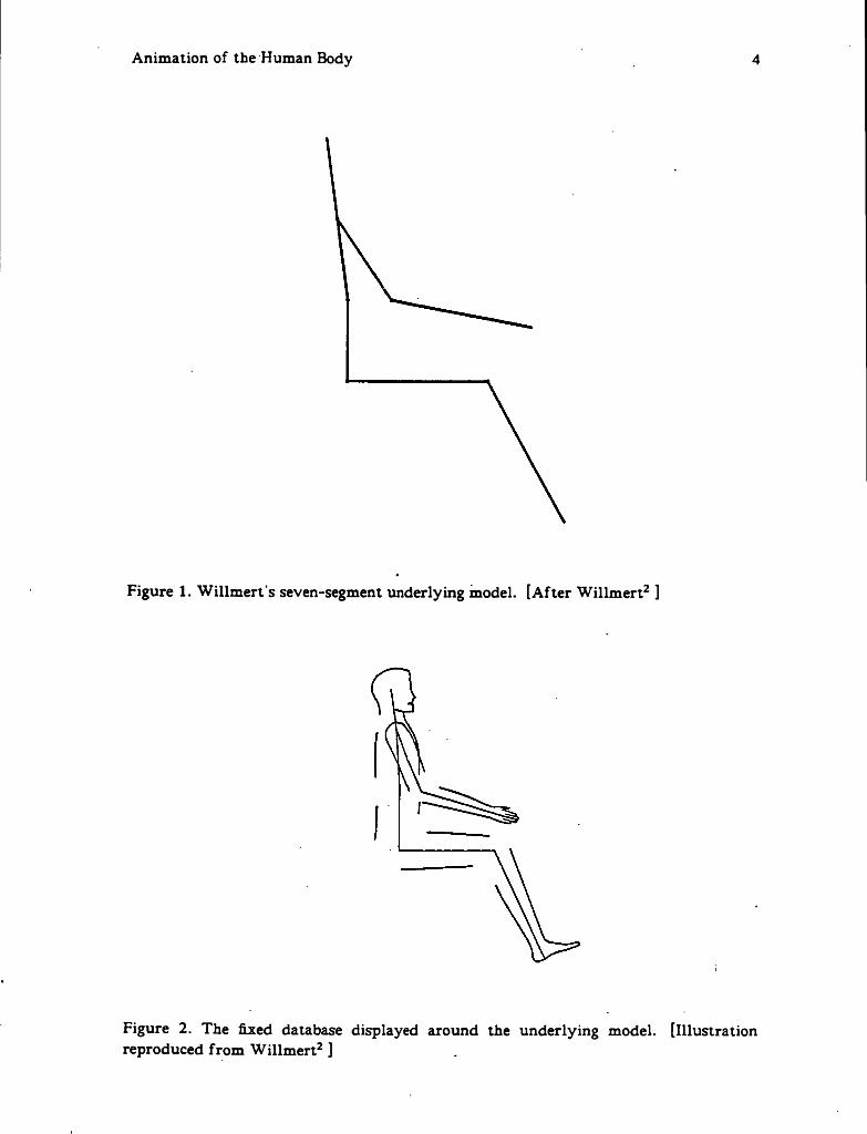
W illmert was later joined by T. E Potter and in 1975 the system had been extended to a three-dimensional body which could be viewed from any position in space3. The extended model of the body employed fifteen different segments corresponding to those in the occupant crash simulation programs in use at the time. Each body segment was defined to be a non-uniform elliptic cylinder (a cylinder capped by parallel ellipses which could have differing centres and major and minor axes. Figure 7). For example, the foot would be a cylinder with an ellipse with a relatively small vertical axis at one end (the toes) and a more circular ellipse at the other end (the ankle) *. A fter projection, the 2-d and 3-d outlines (shadow lines) of the cylinders were drawn and connections between segments formed.

Two new types of joint were employed in addition to those previously described. The first type was the clip and crease, employed where two shadow lines intersect (e.g., at the underside of the knee). The post intersection segments (segments X X —X^Yi and X Y - X 2,Y2 in Figure 8a) are not drawn (clipped) but a crease is added which is drawn


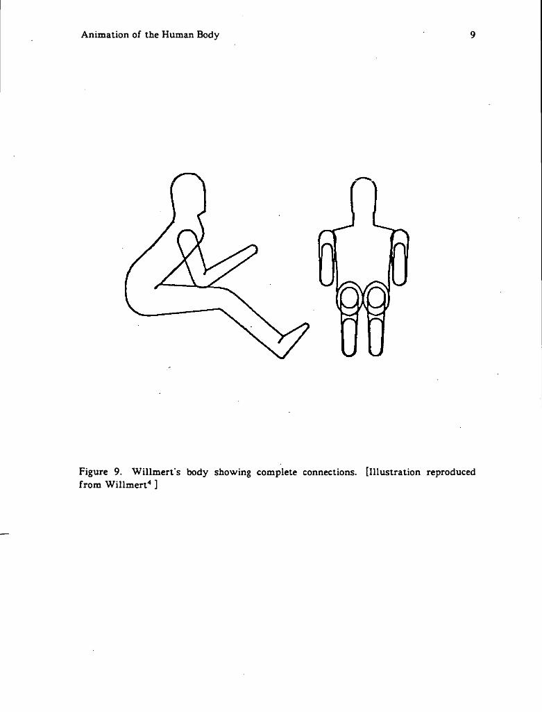
from the intersection to the midpoint of the base of a triangle whose vertices are the shadow line intersection and the two clipped end points (Figure 8b). The fourth type of connection was used when there were more or less than two shadow lines for a segment. This occurs when the radial axis of the cylinder is orthogonal, or nearly so, to the viewing surface. In this case the end ellipses were drawn in their entirety (Figure 9).

According to Willmert. the system occasionally had problems deciding which two shadow lines to join. The solution was to refine the connection criteria to use the surface normals of the plane defined by the two shadow lines of a segment 4. Joining of pairs was then determined by comparing the signs of the surface normals. There was still no hidden line removal employed in the system at that stage.

Later work on the system by Willmert and Potter included conversion to a raster display employing a simple priority algorithm for hidden surface removal (available only in the two dimensional simulations) and the addition of several more joints at the neck for use w ith more sophisticated simulation programs.


Figure 1. W illm ert’s seven-segment underlying model. [After W illmert2 ]

Figure 2. The fixed database displayed around the underlying model, [illustrationreproduced from W illmert2 ]


*3.y3

Figure 3. Linear connection between body parts. [After W illmert2 ]

Figure 4. Circular connection between body parts, [illustration reproduced from W illm ert2 ]


Figure 5. W illm ert’s body displayed with no hidden line processing. [Illustration reproduced from W illmert2 ]

Figure 6. W illm ert's body with only one. lateral, half displayed. [Illustration reproduced from W illm ert2 ]


Figure 7. Top and front views of non-uniform elliptic cylinder. [After W illmert3 ]


8a. Location of points before clipping.

8b. Completed connection.

Figure 8. W illmert's "clip and crease” connection. [After W illmert3 ]


Figure 9. W illmert's body showing complete connections, [illustration reproduced from W illmert4 ]


1.2.

W. A. Fetter

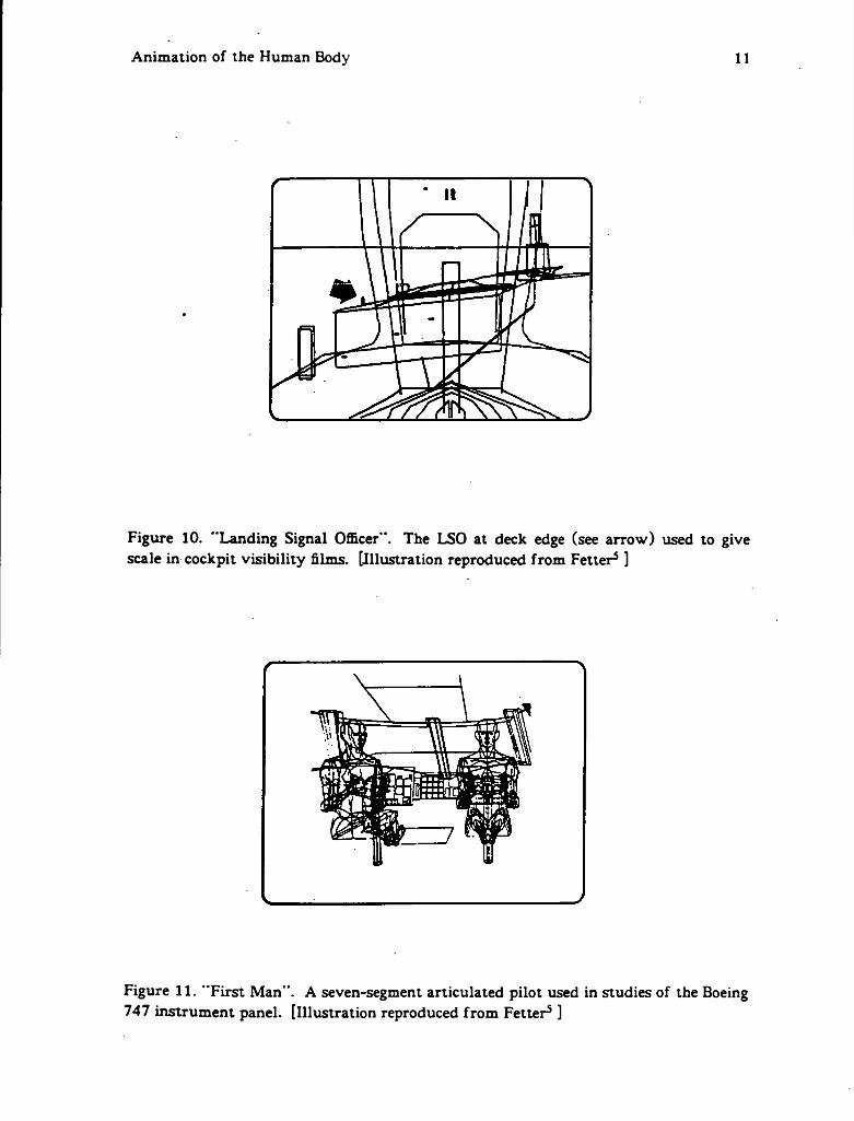
Fetter 5 began work in 1959 on computer generated perspective drawings for the Boeing corporation. His first project, the “Landing Signal Officer", used a fixed database giving the location and scale of the landing signal officer on an aircraft carrier for motion pictures simulating cockpit visibility during landing. This figure was drawn as a crude twelve point silhouette of two dimensional edges (Figure 10). A thirty point figure was available for use in queuing studies. This work culminated in 1968 in the "First Man", which was a figure with seven movable segments articulated at the pelvis, neck, shoulders and elbows (Figure 11). "First Man” was drawn with 3-d surface traces and presented a sufficiently realistic visage to be employed in a 1970 Norelco television commercial (Figure 12).

This work was continued, developing the "Second Man", a refined version of "First Man", which had 19 movable segments and was used to produce movies of running, high jumping, and operating an aircraft control panel (Figure 13).

Fetter then moved to the Carbondale Department of Design at Southern Illinois University where he created the "Third Man” and "Third Woman”. These were a hierarchical series of figures; each element of the series being separated from it's predecessor by an order of magnitude increase in model and visual complexity. The most complex figure (1000 points) was connected as contour lines, the 100-point figure was drawn as boxes, the 10-point figure as a stick figure, and the one-point figure as a dot

.(Figures 14. 15).

While at Carbondale. Fetter used contours to produce the “Fourth Man” and "Fourth Woman”. This system provided for the automatic construction of polygons between contours and could vary the number of contours to produce figures of different complexity. The number of polygons was primarily based on image size and viewing distance, making it possible to construct images having apparently equal visual mass on plotters and equal polygon size on raster displays (Figure 16). The output for raster displays used the Gouraud and (optionally) the Phong shading models.


Figure 10. "Landing Signal Officer". The LSO at deck edge (see arrow) used to give scale in cockpit visibility films. [Illustration reproduced from Fetter5 ]

Figure 11. "First Man”. A seven-segment articulated pilot used in studies of the Boeing 747 instrum ent panel, [illustration reproduced from Fetter5 ]


Figure 12. "First Man". Used in a 1970 Norelco TV commercial, this may have been the first perspective computer graphics television commercial, [illustration reproduced from Fetter5 1

Figure 13. "Second Man”, a more fully articulated 19-segment figure. [Illustration reproduced from Fetter5 ]


Figure 14. “Third Man” a system with an order-of-magnitude progression of complexity. [Illustration reproduced from Fetter5 ]

Figure 15. "Third Woman” used in a 1000-point contour figure. [Illustration reproduced from Fetter5 ]


Figure 16. "Fourth Woman” maintains constant visual density as figure size varies. [Illustration reproduced from Fetter5 ]


13.

T. W. Calvert

Calvert's work began as an effort to provide a more useful display from the output of W olofsky's 6 program to perform computer interpretation of Labanotation 1. The original program, written in Fortran for the IBM S/370. used a 21-joint stick figure (Figure 17) to produce full perspective plots on a Calcomp plotter. The software, translated to Pascal, was running on a PDP-11/34 equipped with an Evans and Sutherland Picture System One by 1978 8.

Since the 11/34 was not equipped with a hardware floating point unit, the frame calculation time was on the order of one frame per second. While this was too slow for real-time display during calculation, it was possible to display precalculated sequences in real-time on the Picture System. It is interesting to note that the stick figure did not suffer from the usual visual ambiguities noted by Herbison-Evans 14 since the modeling software output was a sequence of three dimensional coordinates and the Picture System allowed for the real-time manipulation of the viewing transform. The user could change the position and direction of view and the magnification merely by turning the appropriate dials during viewing, thus providing effective depth queing.

The system was successfully ported to both Apple and Pascal Microengine microcomputers. which, however, were unable to provide the same degree of visual disambiguation because of their limited ability for real-time manipulation. Since it was desirable to use the system in clinical and end user environments (specifically without access to costly, high performance display devices) Calvert then undertook to experiment with alternative output models 9,1 °.

A wire frame polyhedral representation of limbs was tested, but proved to worsen the ambiguity problem when used without real-time perspective capabilities. The next attempt was to use Herbison-Evans’s ellipsoid outline technique, which, while it produced pleasing still pictures (Figure 18). proved computationally too intensive for use on the target hardware. It required approximately two minutes of calculation per frame I0.

The last and most successful approach was to use "Badler's Bubbleman" n . The bubbleman is composed of a jointed stick figure as an underlying model with spheres arranged along the limbs when the figure is rendered (Figure 19). This approach is attractive for a number of reasons. When the output is for previewing purposes or on low capacity equipment, the spheres can be treated as monotone disks with the use of shadow disks employed to provide disambiguation of limb positions, (e.g.. an arm placed in front of the torso is rendered with a darkened outline (Figure 20)). Alternatively when high quality output is desired, the spheres can be rendered efficiently since they are symmetrical in three dimensions. The current model in use employs over eight hundred spheres for high quality output, which is sufficient to faithfully render the contours of the human body.

The polyhedral figure mentioned above is suitable for the purpose of scoring a movement sequence, since this is done on a Silicon Graphics Iris workstation which is fully capable of modifying the viewing transformation and. if desired, filling the polygons, in real-time (providing depth queing) but doesn’t handle spheres as primitive


objects.

_I 'X -iH ^ N |0 $ 9 W P

Figure 17. Calvert's 21-joint stick figure. [Illustration reproduced from Calvert10 ]

Figure 18. Calvert’s "Sausage Person” produced using Herbison-Evans’s NUDES program. [Illustration reproduced from Calvert10 ]


Figure 19. Calvert's "Bubble Person" on an Apple microcomputer. [Illustration reproduced from Calvert10 ]

Figure 20. Calvert’s bubble model using shadow disks to provide visual disambiguation.[Illustration reproduced from Calvert10 ]


1.4.

D. Herbison-Evans

Herbison-Evans's work began with the desire to produce an output processor suitable for a system which would use a computer to interpret dance notation 13. The result of his work was the NUDES system, in which the human body is modelled using ellipsoids that are drawn in outline. NUDES performs hidden line removal but does not draw the actual intersection of ellipsoids. The hidden line algorithm employed consists of solving the quartic equations arising from pairs of ellipsoids

Herbison-Evans notes 13 that ellipsoids provide an efficient representation of humanoids: only 20 ellipsoids, of 100 chords each, requiring the solution of at most

2*202=800

quartic equations, are needed to render a plausible looking humanoid figure. He further notes that this is in contrast to a polyhedral representation which would require

20*i*1002=1052faces and

i.*10104

comparisons using a naive hidden line algorithm. Some of the comparisons can be eliminated by comparing the square of the separation of centres of two candidate ellipsoids w ith the square of the sum of the maximum semi-axis lengths, thus detecting nonintersecting ellipsoid pairs. The complexity is further reduced by detecting completely obscured ellipsoids. Clipping to the viewing surface is done by defining an elliptical viewport. Clipping then becomes just another ellipsoid pair intersection test.

Herbison-Evans has shown 14 that the worst case for a 20-ellipsoid figure is 135,640 m ultiply and divide operations (a test showed the actual number to be 30,325) requiring an estimated ten megaflop computational capacity for real-time calculation and display, or. alternatively, a 150k baud communications channel to a suitably powerful host.

The second phase of Herbison-Evans's work began with the goal of implementing the efficient rendering of shaded ellipsoid solids to model the human body 15. The problem was subdivided into two portions, the identification for each pixel of the visible ellipsoid and the determination of the shade for that pixel given the visible ellipsoid.

The first problem was solved by using an osculating box to first determine at each scan line which ellipsoids might colour pixels of the scanline and then at each pixel to determine which of the reduced set of ellipsoids might colour the pixel. A box was chosen rather than a sphere since tests with a box required no multiplication (versus three for a sphere) and could be more restrictive in many cases.

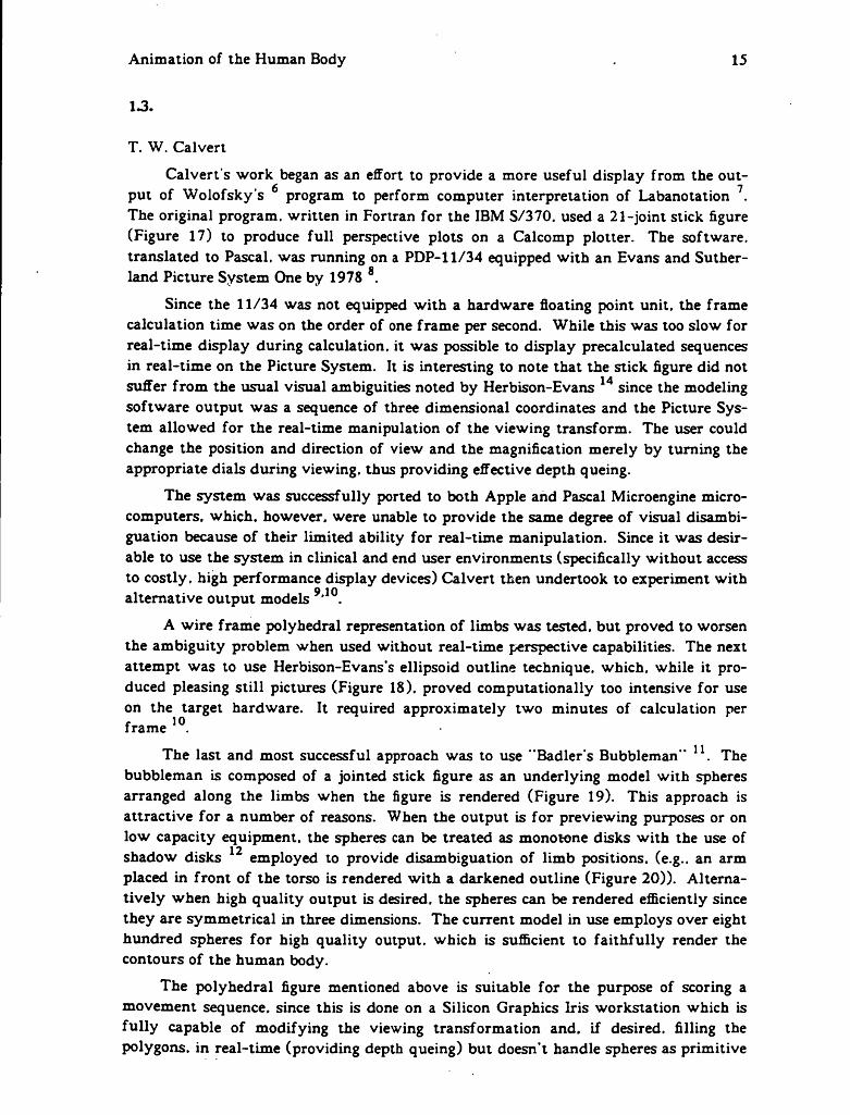
In solving the second problem, he noted that using a vertical illumination source, i.e.. using the Y component of the surface normals rather than the Z component, produced a more natural shading. Efficiency was enhanced by choosing an approximation


for shading that used the moduli of the surface normal components rather than the square root of the sum of squares of the surface normal components (which would have been required to find the true surface normal) which still produced aesthetically acceptable images (Figure 21). Further details of this calculation are given in section 2.8 of this essay.

Figure 21. Ballerina and companion modelled with shaded ellipsoids. [Illustration courtesy of Herbison-Evans]


1.5.

Summary

The general trend of the groups described in this chapter has been a movement away from simple wire frame figures toward rendered surfaces composed of one simple geometric building block (polygons, spheres, or ellipsoids). None of the systems allow the mixing of geometric types, (e.g., a figure composed of both ellipsoids and polyhe- dra). None of the algorithms have the capability of making allowance for, or displaying, the dynamic shape of the body, (e.g., the calves changing shape as steps are taken, which would be desirable in any realistic rendering of human motion). A substantial portion of the intended users of such systems have access only to modest computing resources, however, none of the algorithms/systems described here provide satisfactory performance for this audience.

NUDES

2.1.

Introduction

Herbison-Evans's suite of programs, known collectively as NUDES, allows a user to specify a sequence of movements, for one or more figures constructed of ellipsoids, in a high level language. The user may then view an animation of the movement sequence on a variety of output devices. This chapter describes the major programs which are the components of NUDES, with particular emphasis on the details of RASEL. the program responsible for rendering ellipsoid solids. The general flow of information through the NUDES suite from high level specification to graphics output is given in Figure 22. Further details on the actual use of the programs are given in the UNIX man entry NUDES(lG) available on watcgl in the Computer Graphics Laboratory at the University of Waterloo.

NUDES 22

Figure 22. Flow of information in the NUDES system.

NUDES 23

2.2.

COMPL

COMPL accepts as input a language consisting of high level descriptions of ellipsoids and their movements, similar to the movement description language proposed by Calvert 8. The language is more than a static specification. It provides features necessary for a deterministic simulation of the required movement sequences. COMPL performs syntactic processing of the language and produces a stream of tokens representing the desired sequence that is to be performed by PRFRM. Notable features of the input language are:

- user designated symbolic names for ellipsoids and figures- figures may be joined to other figures and subsequently detached making

such movements as lifts easier to specify- provision is made for parameterized subroutines- movements may have linear and quadratic acceleration profiles- common movements such as spinning, bending, and flexing are available as

atomic operations- basic arithmetic capabilities and user defined variables are provided- Cartesian and angular positions of ellipsoids are available for calculation

purposes in movement procedures during simulation —- the viewing position is specified by the user

23.

PRFRM

PRFRM takes the token stream emitted by COMPL and performs a frame by frame simulation in three space of the movements of the various ellipsoids comprising the scene. The output of PRFRM is a sequence of frames specifying the size, position, and rotation of each ellipsoid during that frame.

2A.

HIDE. VISIB

These programs take the output of PRFRM and project the ellipsoids in each frame to two dimensional outlines. The output of both programs is the position, size and rotation of each ellipse outline for each frame. HIDE also calculates and outputs the arcs of

The interested reader can find further details in “The NUDES Animation Command Language", Don Herbison-Evans, University of Sydney, unpublished.

NUDES 24

ellipsoids which are obscured by other ellipsoids. Figure 18 is an example of the output w ith hidden arcs removed.

2.5.-

SKEL

SKEL takes the output of PRFRM and produces a sequence of frames with stick figures replacing the ellipsoid figures. This is primarily useful for debugging motion sequences where the higher quality and more computationally intensive ellipsoid display is not required.

2.6.

BABY. PLOTL. PRINEL

These programs are primarily output filters that take two dimensional information describing frames as input and prepare output files suited to particular output devices such as printers, plotters, and vector displays.

2.7.

RASEL

RASEL takes the output of PRFRM as input and produces output for display on an AED512 colour raster display. Ellipsoids may interpenetrate and otherwise obscure all or part of the surfaces of other ellipsoids. Hidden surface detection is performed at each pixel and the appropriate surface is rendered according to a simple lighting model. A colour map is also simultaneously calculated and the output is suitable for direct transmission to an AED512.

2.7.1.

Input

The information describing each frame is input to RASEL as a sequence of lines of text, each line describing a single ellipsoid. A line gives the position of the ellipsoid centre in Cartesian coordinates, the length of the three ellipsoid axes and the three Eulerian angles of rotation (latitude, longitude and twist). Numbers are scaled integers with ten Cartesian units corresponding to a one pixel width and one angular unit being equal to one tenth of a degree.

NUDES 25

2.7.2.

Ellipsoid Preprocessing

Prior to a frame being rendered certain preprocessing is performed for each ellipsoid. A rotation matrix R and it's inverse Æ-1 (since R is orthogonal this is trivially given by R -1 = Rr) is determined for each ellipsoid. This is then initially used to determine a bounding box for the rotated ellipsoid by treating the semi-axis lengths as orthogonal vectors and applying R. A diagonal matrix. 1. representing the quadratic form of the unrotated ellipsoid is used in a similarity transform to determine the matrix. L. of the quadratic form of the rotated ellipsoid.

1? 0 00 \ 0 a\

0 0 Xat

L — R l R~l

where ai> a2, and a3 are the lengths of the semiaxes. The coefficients of the polynomial representation of the ellipsoid are then easily calculated from the elements of this matrix as:

Ci — ¿ i.i—

C2 — ¿ 2.2”

¿3.3

(¿2.3)2¿ 3.3

C3 = 7 iL i2- h l h ± )-̂ 3.3

C4 — —2 CiCj — C 3 C 2

C5 — 2C2c2 C3C1

C6 = C1C1 + C2C2 + C3CJC2—1.0

where Cj and c2 are the x and y coordinates of the centre of the ellipse and the following must hold for a point with coordinates x.y to be within the ellipse.

C1X2 + C^y1 + C3xy + C4x + Ctf+Cf,¿ 3,3

In the simple case of an unrotated ellipsoid (R= I. L= 0 this reduces to the familiar

(cj + x)(ci - x) (c2 + y)(c2 - y ) n-----------5--------- + -----------3--------- 1 < va\ ai

Further details of this processing are available both in the RASEL source listing and in

NUDES 26

Herbison-Evans 15. Having performed as much global preprocessing as possible, line by line rendering of the frame is begun.

2.8.

Scan Line Processing

When a new scan line is begun the Y values of each ellipsoid's bounding box are examined and a list is generated specifying all ellipsoids which potentially intercept the scan line. At this point the polynomial representation of each ellipsoid is evaluated as far as possible. As each pixel is rendered in turn the X values of the bounding boxes of each ellipsoid on the list are examined to determine candidacy for the rendering of the pixel. When a candidate ellipsoid is found, the remainder of the polynomial representation is evaluated to determine if the surface of the ellipsoid actually colours the pixel. If this test is passed then the corresponding Z value is determined. A single pixel Z- buffer is used to determine if this Z value is closer to the view point than the Z value for any previous ellipsoid passing the test and, if so. it becomes the new choice for rendering the pixel. This process continues till all candidates have been tested at which point the ellipsoid to be used for rendering (if any) is known.

2.9.

Pixel Rendering

The scheme for determining illumination at the current pixel is computationally simple, yet provides pleasing results. Rather than determine the complete surface normal and then take its product with the illumination vector. RASEL calculates the gradient G at the point and applies the formula

I = A + (1 - A XGy + IIGII

2 IIGII )

where I is the light intensity. A is the ambient light intensity, and Gy is the Y component of the gradient. This provides a smooth transition from the highest intensity point at the "top” of the ellipsoid to the lowest intensity point at the "bottom” of the ellipsoid. The overall intensity is given a small random perturbation in order to reduce contouring problems on displays with a limited number of intensity levels (Herbison- Evans 15) and then combined with the colour information for the ellipsoid to finally render the pixel.

MRASEL

3.1.

Introduction

Having reached the stage of displaying figures constructed of coloured shaded ellipsoids, the natural next step was to add the ability to texture the surface of ellipsoids using arbitrary texture maps. This would allow a more convincing display of figures which appear to be clothed, as well as simplifying the depiction of anatomical features such as hair. The program RASEL served as the base of this effort. This chapter describes the work done to construct MRASEL. an enhanced version of RASEL with texture mapping capabilities.

3.2.

Minor Improvements in RASEL

One subsidiary goal of the work was to have a version of RASEL which was w ritten in the C language (the original being in FORTRAN). While this conversion was being done, minor improvements to the efficiency and functionality of RASEL were implemented. The actual conversion to C was made quite straightforward and relatively painless by the construction of C macros to provide array access with syntax and semantics identical to that of FORTRAN. The use of FORTRAN common blocks was simulated with global static variables in C.

RASEL filled the background with two horizontal bands whose colour and position were fixed at compile time. The C version of RASEL was altered to allow the run-time specification of the number of bands, their position, and their colour(s) to allow for the construction of (slightly) more interesting backdrops. A minor gain in efficiency was effected by moving the lighting calculation out of the loop testing for ellipsoid visibility at each pixel. The lighting calculation is now performed only after the identity of the ellipsoid which colours the pixel has been determined.

While the implementation of complete antialaising of the entire image was beyond the scope of this project, it did prove a simple matter to perform limited antialiasing for the intersection of interpenetrating ellipsoids. When the nearest ellipsoid is determined, a test of the other ellipsoids which also colour the pixel is performed. A cube is defined with faces of the same size as a single pixel and whose near face is at the same position

MRASEL 28

as the ellipsoid which would normally have been chosen to colour the pixel. All ellipsoids whose surfaces lie within this cube are deemed to colour the pixel. The colour for the pixel is arbitrarily chosen as the average of the colours of these ellipsoids at the point of intersection. While this is not correct (the contributions should not be equally weighted), it does provide reasonable results at very low cost. Figure 23 shows two magnified intersecting ellipsoids before and after this processing.

23a. Interpenetrating ellipsoids with no antialiasing.

23b. Interpenetrating ellipsoids with intersection antialiased.Figure 23. An approximation is employed to antialias the intersection of interpenetrating ellipsoids.

MRASEL 29

The final enhancement to RASEL was the provision for device independent output. The FORTRAN version was specifically designed to drive an AED512 raster display. Rather than adapt the code for some specific device existing in the Computer Graphics Laboratory the C version was designed to provide output suitable for use as input to Alan Paeth's suite of raster image manipulation programs 16. This suite of programs provides for output to a variety of raster displays and hardcopy devices, as well as providing facilities for the cropping, rotating, positioning, scaling, etc., of raster images. This has the effect not only of making RASEL somewhat more portable and versatile, but it also resulted in a reduction and simplification of the code.

3 3 .

Texture Mapping

Texture mapping is a technique, first introduced by Catmull . of introducing an arbitrary texture to a surface while it is being rendered. A data object, the texture map. is used to store information about a texture which is then mapped to the surface as it is being rendered. Texture mapping can be conceptually divided into two processes, the definition of a mapping function / between texture space and image space, and filtering the resulting image. Typically the texture map is thought of as a unit square w ith positions on the surface of the square given by two indices, u and v. The texture information, p. at a position (u.v) on the square is then given by

p = p(u.v)

A mapping function. N. is then defined to convert positions in the three dimensional space of the surface being rendered to equivalent positions on the unit square.

(u.v) = N(x.y.z)

The function / . giving the texture information for a given point (x.y,z) is then

f i x . y j ) = />( N ( x . y j ) )

Filtering must then be employed to prevent aliasing artifacts introduced by sampling the texture map.

18Blinn provides an introduction to the use of texture maps for rendering bicubicpatches and the use of lighting models with texture maps. Blinn notes the failure of texture maps to interact suitably with the lighting model used to render a scene which results in textures appearing as if they have been "painted on” an object. He developed the use of texture maps as "bump functions", which produce perturbations in the surface normals of the rendered surface. This results in a realistic rendition of non-smooth three dimensional surfaces even when the underlying surface being mapped is smooth. Dungan 18 * 20 has explored the use of repetitive tiling of portions of an image with a single texture. This has proven useful in. for example, producing scenes of grass and aerial views of forests. He also introduced the technique of variable resolution texture maps

MRASEL 30

(each map differing in size by a power of two from it’s neighbours) as an efficient aid in filtering. Peachey 21 has taken texture mapping a step further through the introduction of texture maps which are defined throughout a region of three-space, thus allowing the depiction of objects whose appearance depends on their internal structure (e.g., a piece of carved wood). His techniques also provide good results when the object being mapped is nonplanar (e.g., a sphere), avoiding the problems of map distortion in regions of curvature. Since the amount of storage required is relatively large if the maps are defined as a three dimensional table the technique realistically requires procedurally defined maps.

A f urther problem with texture mapping is obtaining the maps themselves. While for many purposes it suffices merely to digitize the image of an existing object, or to construct artificial patterns with simple programs, this is not suitable in many cases. Fu22 has investigated syntactic approachs to the generation of texture maps and has demonstrated viable results in the generation of synthetic textures using trees. Fu’s techniques also permit the introduction of local noise emulating the randomness of natural textures. Schweitzer23 has avoided the use of table defined maps altogether and uses simple procedurally defined maps for the purpose of providing depth cues in images through texture mapping. In this case the purpose of the mapping is not to persuade viewers that they are observing a convincing rendition of some real-world object but rather to aid the viewer in percieving the spatial characteristics of the object.

3.4.

Reducing the Problem

A range of techniques are amenable for use in the texture mapping of ellipsoids. A so called "nearest pixel" approach might be employed with, for example, the latitude and longitude of a given position on an ellipsoid surface being used to directly index a simple rectangular map of colour values. While this is attractive since it would be computationally inexpensive, it would be subject to severe aliasing problems at or near the poles of an ellipsoid. More sophisticated methods such as those described in Gardner24 provide good results for actual textures, however they are both computationally expensive and not amenable to producing arbitrary designs such as might be required to simulate the presence of clothing on humanoids constructed of ellipsoids.

As an initial approach it was decided to reduce the problem of texture mapping points on an ellipsoid surface to that of texture mapping points on the surface of a sphere of unit radius. Given an arbitrary pixel at position XeX t on the raster which intersects an ellipsoid surface at Ze. the mapping to the equivalent point Xs. Ys. Zs on the sphere is accomplished in the following manner:

X' = Xe - c 1

r = y.-c2Z‘ = Zf — C3

MRASEL 31

[rrz"] = [ x ' / z ' ] r1

[ xs ys zs ] = [ x r ? ]

1 0 0

0 1a2

0

0 0 1a3

i.e., first the position of the point relative to the ellipsoid centre is determined, then this is “unrotated" using the (already known) inverse of the ellipsoid rotation matrix R. Finally, the point is scaled using the lengths of the ellipsoid semi-axes. Although texture mapping a single known entity, the unit sphere, is substantially simpler than texture mapping an arbitrary ellipsoidal entity, it was still necessary to find a computationally efficient method which would not present severe aliasing problems.

3.5.

MIP Maps

Mip maps are both a data structure and a technique developed by Lance Williams in use at the NYIT Computer Graphics Laboratory since 1979. Mip is an acronym for the latin phrase “multum in parvo” (many things in a small place). When a pixel is rendered using a single simple texture map it may be that the pixel extends over an area of n by m texture map elements. Filtering must be performed to ensure that aliasing does not occur. If a relatively detailed (large) map is being used to texture a small (few pixels) object, the effort required to perform the filtering can be large. Mip mapping is a way of ensuring that n s n ^ l by generating prefiltered texture maps and selecting the appropriate map when a pixel is to be rendered.

The basic idea is to take a base texture map of a size which is a power of two and generate a map of half the size (one quarter the number of elements) be filtering the original map. This process is repeated to generate successively smaller prefiltered maps until a single element map is produced. When an object is to be mapped its size (in pixels) can be used to select an appropriate map such that no more than four map elements need be examined to determine the rendering of the pixel. If the largest map which is smaller than the apparent size of the object is used, the object may be rendered with a slight unnecessary blurring. If the next largest map is employed using simple single element sampling, minor aliasing may occur. Alternatively both interpolation within a map and linear interpolation between the two maps (using the “distance" of the object between the two maps as the interpolation parameter) can be used to ameliorate both the blurring and the aliasing.

MRASE1. 32

As mentioned above, a mip map has a particular structure within memory. The colour components of each map are separated into individual maps such that for a three component colour system all submaps in total have the same storage requirements as the map for a single component at the current level. This allows the submaps to be stored in a single quadrant of a rectangular map and the process can be repeated recursively until the final single element map is generated and only a single element of storage is wasted by the scheme. Figure 24 is a diagrammatic representation of the storage layout used. This scheme is important because given two indices u and v into a particular map. the address of corresponding elements in other maps can be generated using only binary shifts, thus making the technique simple to realize in hardware. It should be obvious from the diagram that the total storage cost of the mip map scheme isonly — greater than that of single map approaches. Further information on mip maps

and their use in both texture mapping and other computer graphics applications can be found in Williams 2S. A variation of mip maps was implemented to perform texture mapping in MRASEL as described below.

MRASEL

Figure 24. Layout of a four level MIP map. [After Williams18 ]

MRASEL 34

3.6.

MRASEL

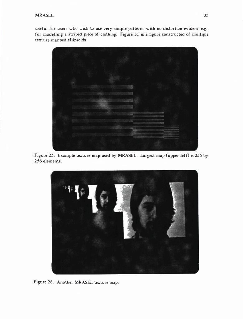
In order to place a practical limit on the secondary storage space occupied by the texture maps an arbitrary decision was made to limit the visual size of all ellipsoids to no greater than 512 pixels. All base maps in use by MRASEL are then of size 512 by 512 by 3 (three byte rgb triples). Since the time required to generate a mip map from a base map of this size is not inconsequential, but the extra space for a mip map is modest. the mip maps were generated by a separate program. MTEXTURE. and kept in a library for use by MRASEL. The maps are actually stored as physically contiguous rgb triples since the time savings provided in element access by the mip map storage scheme are inconsequential compared to the other computations occurring in MRASEL. Each submap is stored separately from the other submaps both in memory and in the file system. This has the advantage of making the maps suitable objects for manipulation by Paeth’s raster programs previously described. Figures 25 and 26 are two examples of maps generated. Each input line to MRASEL specifies a map name rather than a colour for the ellipsoid. As each line is processed, the maximum visual size of the ellipsoid is determined and only the submaps which will be required are loaded into memory, e.g. if an ellipsoids maximum dimension is 55 pixels then only the sub maps of size 64 and smaller are loaded.

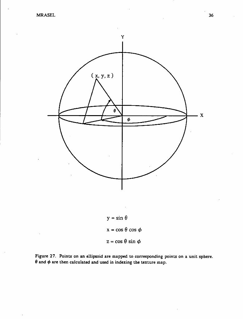
When a pixel is rendered the point on the ellipsoid is mapped to a corresponding point on the unit sphere as previously described. Once this point is known two map indices. 0 and 0 . corresponding to latitude and longitude are generated (Figure 27) as follows.

9 = sin 1 y

0 = s m - - - - - - 75-cos 9

default values are supplied for 0 when cos 0 = 0.

The size of the submap to use is then chosen by

size = min{cos 0. sin 0) maxiaj. a2. <23)

which gives the maximum number of pixels in a vertical line and horizontal line passing through the point. The smallest submap which has size greater than this value is the one chosen to texture the pixel. A simple nearest pixel scheme is then used with 0 and 0 being used as indices into the table to select the value to colour the pixel. Figure 28 and 29 are examples of ellipsoids mapped in this manner. A second mapping is available (selected at compile time) which provides a linear mapping to the sphere by using

0 = sin-1 x

which causes a successively smaller lateral (and central) portion of the map to be used as the poles of the sphere are approached. Figure 30 shows an ellipsoid textured in this manner w ith the same map as used for Figure 28. This alternate mapping seemed

MRASEL 35

useful for users who wish lo use very simple patterns with no distortion evident, e.g.. for modelling a striped piece of clothing. Figure 31 is a figure constructed of multiple texture mapped ellipsoids.

Figure 25. Example texture map used by MRASEL. Largest map (upper left) is 256 by 256 elements.

Figure 26. Another MRASEL texture map.

MRASEL 36

Y

y = sin 9

x = cos 9 cos 0

z = cos 9 sin 0

Figure 27. Points on an ellipsoid are mapped to corresponding points on a unit sphere. 6 and <f> are then calculated and used in indexing the texture map.

MRASE1. 37

Figure 28. Vertical stripes mapped to an almost spherical ellipsoid.

Figure 29. A map of finer vertical stripes mapped to a rotated ellipsoid.

MRASEL 38

Figure 30. The same texture map and ellipsoid as in Figure 28 but using the alternate mapping described in section 3.5.

Figure 31. A caterpillar rendered using texture maps generated by digitizing the coat of a dog.

MRASEI 39

3.7.

Future Improvements

There are a number of potential areas for improving the performance and functionality of MRASEL. The functions responsible for allocating texture table storage and reading in the texture maps are overly simplistic. No attempt is made to determine if two or more ellipsoids employ the same texture map. Storage is not freed once an ellipsoid has been completely processed. Ideally, the program would recognize cases where the same map is employed by two or more ellipsoids and only create one instance of the map. As well, a map need not be allocated storage until the first scan line is processed where it is used. When the map is no longer needed it’s storage should be freed. Since the mip maps employed can be up to 780k in size, this could afford substantial storage economies as well as decreasing I/O requirements. The use of simple bands for background is limiting; it would not be difficult to allow a file containing an arbitrary raster image to be used as the source of the background.

The trigonometric evaluations required to determine the correct texture map entry for a given point on the unit sphere are relatively expensive. However, the degree of accuracy required in this application is relatively low and the use of modestly sized tables should allow for substantial speedup in this area.

Since actual ellipsoid intersections are antialiased, the only remaining cases requiring antialiasing are the intersection of the background with an ellipsoid, and two or more ellipsoids overlapping at a pixel but not interpenetrating. In both cases at least one edge of an ellipsoid projection is involved. Since every ellipsoid which is active on a scan line has on its edges the first and last pixel it intersects on the scan line, it would be relatively easy to maintain two flags for each ellipsoid that would be initialized at the beginning of each scan line and updated when its first and last pixels are processed. In this manner the edge intersections could be recognized efficiently and the antialiasing accomplished relatively cheaply.

Inter- and intra-level interpolation in the mip map was not deemed to be necessary in this initial attempt at providing texture mapping for NUDES. Finally, the one drawback to mip maps is that they employ a symmetrical filter — each of the submaps is filtered equally in X and Y. Crow 26 has proposed an alternative, summed area tables, that allows for asymmetrical filtering at no significant increase in computational cost. However this technique places much higher demands on storage facilities, a 512 by 512 rgb map would require a 512 by 512 map for each colour component, where each entry would require 26 bits for a total increase in storage requirements of 3.25 as compared to 1.33 for mip maps. Given the size of the tables, and the fact that unless the ellipsoid’s semiaxes were aligned with the axes of the coordinate system the access to the texture map would be essentially random (from the point of view of a virtual memory system paging algorithm), this could lead to thrashing. Since both the changes mentioned in this paragraph would increase time and/or space requirements significantly, they should probably not be implemented until sufficient use of the system is made to determine their desirability — the facilities already provided may prove adequate for the relatively limited texture mapping requirements of the system.

REFERENCES

1K. D. W illmert. "Visualizing Human Body Motion Simulations”. IEEE Computer Graphics and applications. Vol. 2, No. 9, Nov. 1982. pp. 35-38.

2K. D. W illmert. "Occupant Model For Human Motion", Dept, of Mechanical and Industrial Engineering. Clarkson College. Potsdam. N.Y. Report No. MIE-009, July 1974.

3T. E. Potter and K. D. Willmert. "Three Dimensional Human Display Model” . Dept, of Mechanical and Industrial Engineering. Clarkson College, Potsdam. N.Y. Report No. MIE-010. July 1975.

4 -K. D. W illmert and T. E. Potter. "An Improved Human Display Model for Occupant Crash Simulation Programs", Dept, of Mechanical and Industrial Engineering, Clarkson College. Potsdam. N.Y., Report No. MIE-018, April 1976.

5W. A. Fetter. "A Progression of Human Figures Simulated by Computer Graphics". IEEE Computer Graphics and applications. Vol. 2. No. 9. Nov. 1982, pp 9-13.

6Z. Wolofsky. "Computer Interpretation of Selected Labanotation Commands". MSc. thesis. Kinesiology Dept., Simon Fraser University. 1974.

7A. Hutchinson, "Labanotation", 2nd Ed.. Theatre Arts Books. New York 1960.

8T. W. Calvert and J. Chapman. "Notation of Movement with Computer Assistance", Proc. ACM Annual Conf.. Vol. 2, 1978. pp 731-736.

REFERENCES 41

9T. W. Calvert. J. Chapman, and A. Patla. "The Integration of Subjective and Objective Data In Animation of Human Movement". Computer Graphics. Vol. 14. No. 3. Aug. 1980. pp 198-205.

10T. W. Calvert. J. Chapman, and A. Patla. “Aspects of the Kinematic Simulation of Human Movement” , IEEE Computer Graphics and applications. Vol. 2. No. 9. Nov. 1982. pp 41-50.

11N. I. Badler, J. O’Rourke, and H. Toltzis. “A Spherical Representation of a Human Body for Visualizing Movement”. Proc. IEEE. Vol. 67. No. 10. Oct. 1979. pp 1397-1402.

12K. Knowlton. “Computer-Aided Definition. Manipulation, and Depiction of Objects Composed of Spheres” . Computer Graphics, Vol. 15, No. 2. Apr. 1981, pp 48-71.

13D. Herbison-Evans. "NUDES 2: A Numeric U tility Displaying Ellipsoid Solids. Version 2” . Computer Graphics, Vol. 12. No. 3. Aug. 1978. pp 354-356.

14D. Herbison-Evans. “Real-Time Animation of Human- Figure Drawings with Hidden Lines Omitted". IEEE Computer Graphics and applications. Vol. 2. No. 9, Nov. 1982, pp 27-33.

15D. Herbison-Evans. "Rapid Raster Ellipsoid Shading” , Computer Graphics. Vol. 13, No. 4. Feb. 1980. pp 355-361.

16A. W. Paeth. “A Comprehensive Raster Toolkit Presented through Design and Example”. M. Math Essay, University of Waterloo. April 1985.

17E. Cat mull. "A Subdivision Algorithm for Computer Display of Curved Surfaces", Ph.D. dissertation. University of Utah. 1974.

18J. F. Blinn and M. E. Newell. "Texture and Reflection in Computer Generated Images” . Communications o f the ACM. Vol. 19. No. 10. Oct. 1976. pp 542-547.

19J. F. Blinn. Simulation of Wrinkled Surfaces”. Computer Graphics. Vol. 12. No. 3, Aug. 1978, pp 286-292.

REFERENCES 42

20W. Dungan Jr., A. Stenger. and G. Sutty. "Texture Tile Considerations for Raster Graphics". Computer Graphics. Vol. 12. No. 3, Aug. 1978. pp 130-134.

21D. R. Peachey. “Solid Texturing of Complex Surfaces” . Computer Graphics, Vol. 19, No. 3. July 1985. pp 279-286.

22K. S. Fu and S. Y. Lu. "Computer Generation of Texture Using a Syntactic Approach", ComputerGraphics. Vol. 12. No. 3. Aug. 1978, pp 147-152.

23D. Schweitzer. "Artificial Texturing: An Aid to Surface Visualization” , Computer Graphics. Vol. 17. No. 3. July 1983. pp 23-29.

24G. Y. Gardner. "Simulation of Natural Scenes Using Textured Quadric Surfaces", Computer Graphics. Vol. 18. No. 3. July 1984. pp 11-20.

25L. Williams. "Pyramidal Parametrics”. Computer Graphics. Vol. 17. No. 3. July 1983,pp 1- 1 1 .

26F. C. Crow. "Summed-Area Tables for Texture Mapping” . Computer Graphics. Vol. 18. No. 3. July 1984. pp 207-212.

APPENDIX I : Creating An Image W ith MRASEL

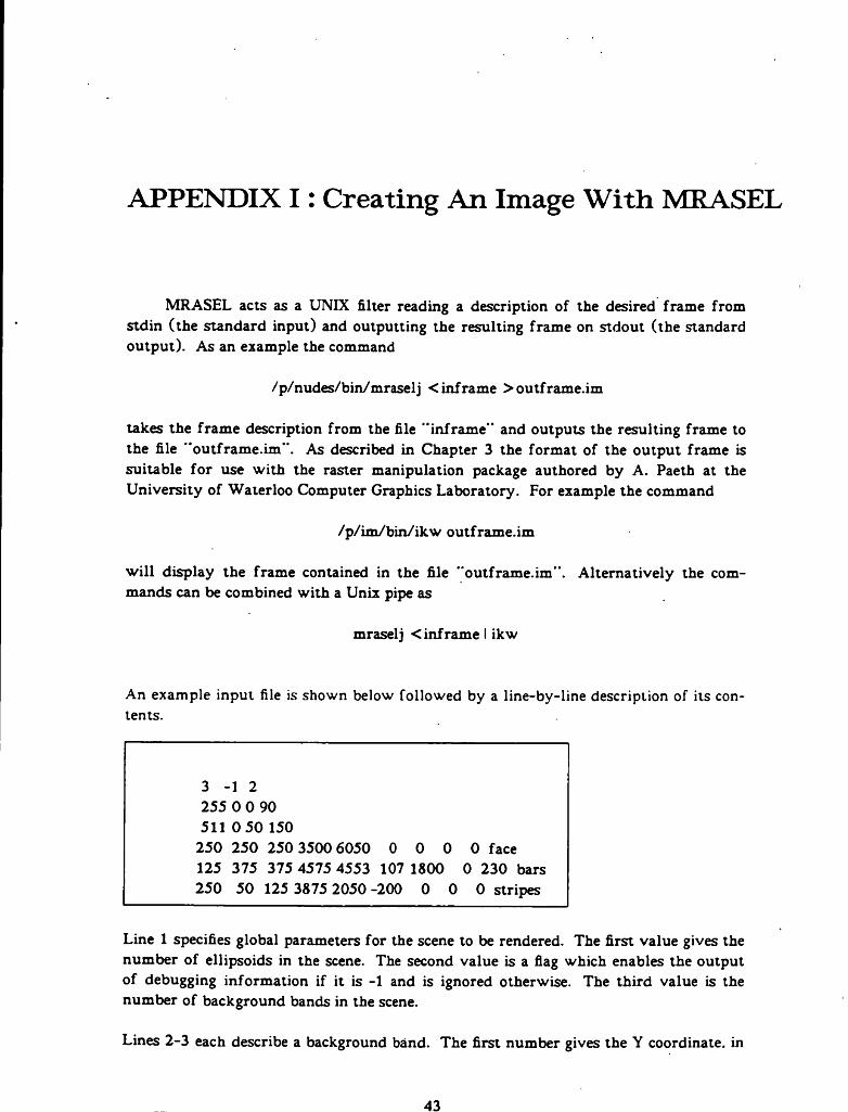
MRASEL acts as a UNIX filter reading a description of the desired frame from stdin (the standard input) and outputting the resulting frame on stdout (the standard output). As an example the command

/p/nudes/bin/mraselj < inframe >outframe.im

takes the frame description from the file "inframe” and outputs the resulting frame to the file "outframe.im". As described in Chapter 3 the format of the output frame is suitable for use with the raster manipulation package authored by A. Paeth at the University of Waterloo Computer Graphics Laboratory. For example the command

/p/im /bin/ikw outframe.im

will display the frame contained in the file "outframe.im". Alternatively the commands can be combined with a Unix pipe as

mraselj < inframe I ikw

An example input file is shown below followed by a line-by-line description of its contents.

3 - 1 2 255 0 0 90 511 0 50 150

250 250 250 3500 6050 0 0 0 0 face125 375 375 4575 4553 107 1800 0 230 bars250 50 125 3875 2050 -200 0 0 0 stripes

Line 1 specifies global parameters for the scene to be rendered. The first value gives the number of ellipsoids in the scene. The second value is a flag which enables the output of debugging information if it is -1 and is ignored otherwise. The third value is the number of background bands in the scene.

Lines 2-3 each describe a background band. The first number gives the Y coordinate, in

43

APPENDIX I : Creating An Image With MRASEL 44

the range 0 to 511. of the last position at which the band should be displayed. The last three numbers give the red, green, and blue components of the band colour, each in the range 0 to 255. In the example there will be a dark blue band in the top half of the screen and a lighter greenish-blue in the bottom half of the screen.

Lines 4-6 each describe an ellipsoid. The first three numbers give the lengths of the three semiaxes of the ellipsoid, in pixels. The next three numbers specify the position on the screen of the centre of the ellipsoid in tenths of pixels. The next three numbers give the Eulerian rotation of the ellipsoid in tenths of degrees. The name at the end of the line is name of the map to be used to texture the ellipsoid.

MRASEL expects the maps named in the input file to be found in the current working directory. The program MTEXTURE is used to generate a set of maps from an input base map. MTEXTURE is used as follows:

mtexture < basemap mapname

The file "basemap” is an input map consisting of 262,154 (5122) three byte rgb triples. The first triple corresponds to the upper left comer of the map and the last triple to the lower right comer of the map. Files of this format can be generated from standard Iko- nas image files by Alan Paeth’s raster manipulation program "imheadoff” . MTEXTURE creates ten files ( mapname.512, mapname.256.... , mapname.l containing the appropriate antialiased texture maps) in the current working directory.

The utility program SHOWMAP can be used to create a single file of the ninesmallest maps (mapname.256. mapname.128........ mapname.l ) which is suitable fordirect display by Paeth’s raster programs. This can be useful to see the extent to which antialiasing has blurred the original image. SHOWMAP is used as follows:

showmap mapname >outfile

The input files should be in the current working directory.

APPENDIX n : Source Code

The necessary files to build the programs are located on watcgl in the University of Waterloo Computer Graphics Lab. The files are:

/ p/nudes/sources/raselj.c — C version of RASEL.

/p/nudes/sources/mraselj.c — MRASEL source code.

/p/nudes/sources/mtexture.c — MTEXTURE source code.

/p/nudes/sources/showmap.c — SHOWMAP source code.

/p/nudes/sources/makefile — Makefile for producing the various programs (see below)

Each of these programs is simply compiled using the C compiler.

Additionally. MRASEL may be compiled with two different flags defined. If DEBUG is defined then a number of statements are compiled which send status information to stderr when the program is run. If LINEAR is defined then the linear mapping described in chapter 3 is implemented. These two flags may be defined singly or in combination. It is also necessary to include the math library. As an example, the following command

cc -DDEBUG mraseli.c -lm -o DMRASEL

compiles a version of MRASEL that produces debugging information and names the executable DMRASEL. The following page shows a makefile suitable lo r producing all versions of the program.

APPENDIX II : Source Code 46

## This makefile produces executable programs from (the C version of)# RASEL, MRASEL and the associated utility programs. Sources are# expected to be in the current working directory and the resulting# executables are left in the current working directory.#CFLAGS = -O

RASEL : raseli.c -cc $(CFLAGS) raseli.c -o RASEL

# produce executable of MTEXTURE (program to make texture maps) MTEXTURE: mtexture.c

cc $(CFLAGS) mtexture.c -o maps/MTEXTURE

# produce executable of SHOWMAP (program to display texture maps) SHOWMAP: showmap.c

cc $(CFLAGS) maps/showmap.c -o maps/SHOWMAP

#produce executable of MRASEL MRASEL : mraseli.c

cc $( CFLAGS) mraseli.c -o MRASEL

#produce executable of MRASEL with the debugging option enabled MRASELD : mraseli.c

cc -DDEBUG mraseli.c -o MRASELD

#produce executable of MRASEL with LINEAR mapping option enabled MRASELL : mraseli.c

cc $(CFLAGS) -DLINEAR mraseli.c -o MRASELL

#produce executable of MRASEL with both LINEAR and debugging options #enabledMRASELLD : mraseli.c

cc -DLINEAR -DDEBUG mraseli.c -o MRASELLD

Texture Mapped Ellipsoids for Human Animation

Documents

Transcript of Texture Mapped Ellipsoids for Human Animation