Av. Bandeirantes, 3900 - Monte Alegre - CEP: 14040-905 - Ribeirão Preto-SP

Fone (16) 3602-4331/Fax (16) 3602-3884 - e-mail: cebelima@usp.br site:www.fearp.usp.br

Faculdade de Economia,

Administração e Contabilidade

de Ribeirão Preto

Universidade de São Paulo

Texto para Discussão

Série Economia

TD-E 05 / 2014

More of Less isn’t Less of More: Assessing Environmental Impacts

of Genetically Modified Seeds

in Brazilian Agriculture Renato Nunes de Lima Seixas

Av. Bandeirantes, 3900 - Monte Alegre - CEP: 14040-905 - Ribeirão Preto - SP

Fone (16) 3602-4331/Fax (16) 3602-3884 - e-mail: cebelima@usp.br site: www.fearp.usp.br

Av. Bandeirantes, 3900 - Monte Alegre - CEP: 14040-905 - Ribeirão Preto-SP

Fone (16) 3602-4331/Fax (16) 3602-3884 - e-mail: cebelima@usp.br site:www.fearp.usp.br

Universidade de São Paulo

Faculdade de Economia, Administração e Contabilidade

de Ribeirão Preto

Reitor da Universidade de São Paulo

Marco Antonio Zago

Diretor da FEA-RP/USP

Sigismundo Bialoskorski Neto

Chefe do Departamento de Administração

Sonia Valle Walter Borges de Oliveira

Chefe do Departamento de Contabilidade

Adriana Maria Procópio de Araújo

Chefe do Departamento de Economia

Renato Leite Marcondes

CONSELHO EDITORIAL

Comissão de Pesquisa da FEA-RP/USP

Faculdade de Economia, Administração e Contabilidade de Ribeirão Preto

Avenida dos Bandeirantes,3900

14040-905 Ribeirão Preto – SP A série TEXTO PARA DISCUSSÃO tem como objetivo divulgar: i) resultados de trabalhos em desenvolvimento na FEA-RP/USP; ii) trabalhos de pesquisadores de outras instituições considerados de relevância dadas as linhas de pesquisa da instituição. Veja o site da Comissão de Pesquisa em www.cpq.fearp.usp.br. Informações: e-mail: cpq@fearp.usp.br

More of Less isn’t Less of More: Assessing

Environmental Impacts of Genetically Modified Seeds

in Brazilian Agriculture

Job Market Paper

Renato Seixas

José Maria Silveira

We investigate the environmental effects due to pesticides for two different genetically modified (GM) seeds: insect resistant (IR) cotton and herbicide tolerant (HT) soybeans. Using an agricultural production model of a profit maximizing competitive farm, we derive predictions that IR trait decreases the amount of insecticides used and HT trait increases the amount of less toxic herbicides. While the environmental impact of pesticides for IR seeds is lower, for the HT seeds the testable predictions are ambiguous: scale as substitution effects can lead to higher environmental impacts. We use a dataset on commercial farms use of pesticides and biotechnology in Brazil to document environmental effects of GM traits. We explore within-farm variation for farmers planting conventional and GM seeds to identify the effect of adoption on the environmental impact of pesticides measured as quantity of active ingredients of chemicals and the Environmental Impact Quotient index. The findings show that the IR trait reduces the environmental impact of insecticides and the HT trait increases environmental impact due to weak substitution among herbicides of different toxicity levels. Keywords: Brazil, Agriculture, Environmental Impact, Genetically Modified Seeds, Herbicide Tolerant Soybeans, Insect Resistant Cotton, Pesticides

May, 2014

We thank Anderson Galvão from Celeres, for kindly providing the dataset, and comments from David Zilberman, Sofia Villas Boas, Max Auffhammer, Christian Traeger, Jeff Perloff, Avery Cohn, Marieke Kleemans, Manuel Barron, Kyle Emerick, Sam Heft-Neal, participants in the ERE seminar and development lunch at UC Berkeley and at the 17th ICABR conference “Innovation and Policy for the Bioeconomy”. Financial support from CAPES/Fulbright PhD fellowship (grant 2256-08-8) is greatly acknowledged. All remaining errors are ours. PhD candidate at ARE/UC Berkeley. Corresponding author: rnlseixas@berkeley.edu . IE/UNICAMP

1

1 INTRODUCTION

The research agenda on food supply has received increased attention since the global food crisis

of 2008. In this context, genetically modified (GM) seeds have been considered one of the

major breakthroughs in technological innovation for agricultural systems and have been

promoted as an effective tool for control of agricultural pests and food supply expansion. Their

relevance can also be measured by the wide spam of controversial issues that have been raised

in the related literature since their introduction. Those involve: intellectual property rights over

organisms, productivity effects, economic returns, consumer safety, welfare and income

distribution, and environmental effects (Qaim, 2009). Potential sources of related economic

gains include reduced crop losses, reduced expenditure on pest control, farmworker safety and

health conditions, and lower variability of output (Sexton & Zilberman, 2012).

In the environmental front, benefits from adoption of GM seeds have been argued based

on findings about pesticide use and agricultural practices. Insect resistant (IR) cotton has been

found to reduce the use of insecticides and therefore to produce environmental, health and

safety gains (Qaim & Zilberman, 2003; Qaim & de Janvry, 2005; Huang, Hu, Rozelle, Qiao, &

Pray, 2002). Herbicide tolerant (HT) soybeans have been found to change the mix of herbicides

applied towards less toxic products and to allow the use of no-till cultivation techniques, leading

researchers to conclude (tentatively) that they also produce environmental benefits (Fernandez-

Cornejo, Klotz-Ingram, & Jans, 2002; Qaim & Traxler, 2005; Brookes & Barfoot, 2012).

This paper addresses the environmental impacts, associated with the use of pesticides,

resulting from adoption of GM seeds in Brazil. First, we use a model of a profit maximizing

competitive farm to show how the interaction of different GM traits (HT and IR) affects the

optimal use of pesticides, more specifically herbicides and insecticides. We show that the IR

trait works as substitute for insecticides and hence reduces the optimal use of these products.

The resulting environmental effect is straightforward: less insecticide usage leads to lower

environmental impact. The HT trait, on the other hand, works as a complement to herbicides,

2

specifically to glyphosate1, and induces an increase in the use of this product. The resulting

environmental impact is ambiguous and we argue that it depends on the interplay of a

substitution effect, between herbicides of different toxicity levels, and a scale effect, of

increased use of glyphosate.

In the empirical analysis, we use a unique farm-level dataset that documents adoption of

GM seeds and pesticide use between 2009 and 2011 for cotton, maize and soybeans cultivation

by commercial farms in Brazil to present the first reduced form models estimates of

environmental effects of two different biotechnology traits: IR cotton and HT soybeans. The

dataset is disaggregated by fields, within a farm, cultivated with conventional or GM seeds. In

other words, for each farm, we have potentially multiple observations related to fields cultivated

with conventional or GM seeds. This setup allows us to use within-farm variation for farmers

that plant both conventional and GM seeds to identify the effect of adoption on the

environmental impact of pesticides.

We measure the environment impact as two outcome variables: quantity (kg/ha) of active

ingredients of chemicals and the Environmental Impact Quotient (EIQ) index (Kovach,

Petzoldt, Degnil, & Tette, 1992). This measure of environmental impact of pesticides was

designed to capture risks associated with both toxicity levels and exposure to chemical

pesticides on three components of agricultural systems: farmworker, consumer and ecological.

Hence, the EIQ index gives a more complete picture than just the composition of the mix of

pesticides used allowing for an adequate weighting of pesticides of different toxicity levels.

This represents a big advancement over previous studies that only documents increased use of

less toxic pesticides for HT soybeans and so cannot capture environmental effects due to

substation and scale effects. Concretely, if the increase in the use of less toxic herbicides is not

accompanied by a sufficient decrease in more toxic ones (substitution effect) or if the increase

1 The United States Environmental Protection Agency (EPA) considers glyphosate as a pesticide of toxicity level III, in a scale from I (most toxic) to IV (practically nontoxic), requiring products that carry it as active ingredients to obey safety conditions for manipulation such as protective clothing and no re-entrance in treated fields for 4 hours (United States Environmental Protection Agency, 1993). In the classification of environmental impacts, glyphosate is in the 145o position out of 178 active ingredients classified (Kovach, Petzoldt, Degnil, & Tette, 1992).

3

in less toxic is much higher than the decrease in more toxic ones (scale effect), them the new

mix of herbicides induced by HT seeds can be more harmful than the one induced by

conventional seeds. The EIQ index calculated for field operations allows us to adequately

weight pesticides of different toxicity levels and gets around the difficulties of looking only at

the mix of pesticides used.

Our findings show that, as expected, adoption of cotton seeds with IR trait reduces the

amount of insecticides used by 24.2% and, consequently, the environmental impact index by

23.4% when compared with fields cultivated with conventional seeds. For soybean seeds with

HT traits, however, although farmers use more of less toxic herbicides, we estimate that the net

environmental impact is higher than for conventional seeds. We find that adoption of these

seeds cause an increase of 44.2% of herbicides use and a corresponding 35.6% increase in the

EIQ index when compared with fields cultivated with conventional seeds. Moreover, we

estimate that the increase in the use of herbicides of low toxicity levels is twelvefold the

decrease in the use of herbicides of high toxicity levels. This result indicates that the main

mechanism driving the findings on the EIQ index is the weak substitution among herbicides of

different toxicity levels.

Those results are not inconsistent with the literature on environmental effects of GM

seeds. For IR cotton, Qaim & Zilberman (2003), Qaim & de Janvry (2005) and Huan et al.

(2005) find significant reductions in average use of insecticides in India, Argentina and China,

respectively. For HT soybeans, Fernandez-Cornejo et al. (2002) and Qaim & Traxler (2005)

find increases in the use of glyphosate and some reduction in the use of more toxic herbicides,

which leads them to conclude for environmental benefits due to the adoption of this type of

seed. Our results confirm the environmental gains from IR cotton but suggest that the findings

on the environmental effects of HT soybeans have been misled by relying solely on the change

in the mix of herbicides used.

The rest of the paper is organized as follows. Section 2 introduces a quick background on

biotechnology and its regulation in Brazil. Section 3 describes the theoretical framework that

4

informs the testable hypotheses. Section 4 describes the dataset and presents the empirical

strategy. Section 5 shows the results obtained and section 6 concludes.

2. SOME BACKGROUND ON BIOTECHNOLOGY AND REGULATION

Since the mid 1990’s, when first-generation GM seeds were commercially introduced, adoption

by farmers has grown steadily in industrialized and developing countries as they provide an

alternative and more convenient way of reducing pest damage2 (Figure 1). By 2008, 13.3

million farmers dedicated 8% of total cropland (12.5 million ha) to the cultivation of GM seeds.

The leading countries in terms of share of cultivated are in 2009 were the US (50%), Argentina

(17%), Brazil (13%), India (6%), Canada (6%) and China (3%) (James, 2008).

The main traits that have been introduced in first generation GM seeds correspond to the

herbicide tolerant (HT) and insect resistant (IR) technologies. The focus of this paper relies on

HT soybeans and IR cotton.

Soybeans are an annual crop, which means the plant life cycle (seed-flower-seed) last one

season only. Weeds are strong competitors with soybean plants for nutrients, water and sunlight.

Field infestation can produce yield losses since soybeans are sensitive to moisture and light

deficiency, especially in the emergency phase before the plant canopy closes and puts it in

advantage against weeds. Weed control techniques have evolved from traditional mechanical

methods to herbicides applications introduced in the 1960’s (Carpenter & Gianessi, 1999). The

first generation of herbicides were known as pre-emergence since they have to applied before

planting as weed burn down. Following application, farmers still had to rely on mechanical

control until soybean canopy closes and shades competing weeds. Starting in the 1980’s,

postemergence herbicides were introduced and allowed growers to use chemical control of

weeds instead of mechanical tillage over the growing season. This change made possible to

increase the planted acreage since herbicide-based weed control is more efficient than

2 Second-generation GM seeds display quality improvements in nutritional contents and third generation are designed for pharmaceutical (vaccines and antibodies) and industrial (enzymes and biodegradable plastics) applications.

5

mechanical tillage. Postemergence herbicides also make possible to narrow the space between

plant rows in the fields which increases yields as a result of a more efficient use of space.

Nevertheless, postemergence herbicides also have drawbacks that limit their application

and effectiveness in highly infested areas. These include: potential for crop injury in the form of

stunted growth or yellowing/burning leaves, development of herbicide resistant weeds and

residual effects on soil that might be deleterious to rotation of crops (Carpenter & Gianessi,

1999).

Soybean seeds engineered with HT traits were introduced in 1996 under the commercial

name Roundup Ready. They’re the result of the transfer of part of the genetic code of a soil

bacterium, Agrobacterium tumefaciens, which allow the plant to metabolize the herbicide

glyphosate (Roundup). In 1998, soybean varieties tolerant to the herbicide glufosinate were

introduced under the commercial name Liberty Link. Those herbicides target a large variety of

broad-leaf and grass weeds species but cause severe damages to conventional crops when

applied after germination (post-emergent weed control). The primary reason given for the rapid

diffusion rated of those seeds, notably the Roundup Ready ones, is the simplicity of the

glyphosate-based weed control, which allows farmers to concentrate on one herbicide to control

a wide range of weeds. In addition, it also proved more convenient for farmers since the timing

of application can be extended beyond soybean flowering and the maximum size of weeds that

are effectively controlled is higher compared with other postemergence herbicides (Carpenter &

Gianessi, 1999). Herbicide related cost savings have also been pointed as one of the reasons for

adoption, since glyphosate patent expired in the year of 2000, allowing the entry of new

suppliers and lowering the price of glyphosate-based herbicides (Qaim, 2009). Hence, from the

point of view of farmers, HT soybeans have been shown to be both technically and

economically advantageous, which explains the rapid diffusion that they have displayed.

IR seeds3 are engineered to produce a natural toxin produced by the soil bacterium

Bacillus thuringiensis (Bt), which is lethal to a number of bollworms pests but not to mammals.

IR crops have also been deemed technically and economically efficient for producers. The most

3 Also referred in the literature as Bt seeds.

6

straightforward reason is related to savings in insecticides applications (which spams from labor

time to savings in machinery use, aerial spraying etc.) targeted to bollworm killing. Specifically,

in regions with high insect infestation, typical less developed countries in tropical weather

regions, and high rates of insecticide use, the potential for reduction is conversely high (Qaim &

Zilberman, 2003). Positive yield effects have also been noted since the Bt toxin compound on

the insecticide effect reducing losses due to insect attack (Qaim, 2009). In fact, it has been

argued that yield and insecticide reduction effects are closely related: farmers facing high pest

pressure and still using low rates of insecticides

Besides, it has also been considered a more efficient tool for managing the risk of pest

attack than reactive application of insecticides (Crost & Shankar, 2008) which has been

translated in reduced crop insurance premium (Brookes & Barfoot, 2012). Other benefits

pointed relate to improve safety conditions for farm workers and shorter growing season

(Brookes & Barfoot, 2012).

Crops that have been engineered with the above traits are: cotton, maize, rapeseed and

soybean. More recently, some crops have also been engineered with both HT and IR traits and

are commonly referred as stacked varieties. The most used technology is HT in soybeans, which

corresponded to 53% of GM seeds planted area in 2008 and is grown mostly in US, Argentina

and Brazil. The second-most used technology is HT and IR maize, which accounted for 30% of

GM seeds planted area in 2008 (James, 2008).

Despite the production benefits, consumers have shown suspicious attitudes regarding the

health and environmental safety of products originated from GM seeds and government

regulation has ranged from cautionary permission to complete ban. The European Union, for

instance, imposed a ban on GM seeds that was lifted in 2008. Also, GM seeds uses have been

restricted to animal feed and fiber uses and producers are required to segregate GM crops output

throughout the supply chain (Sexton & Zilberman, 2012). Other concerns relate to the

undermining of traditional knowledge systems in developing countries and the possibility of

monopolization of seed markets by large multinational companies and exploitation of small

farmers (Sharma, 2004).

7

The regulation of GM seeds in Brazil originates in the first Biosafety Law from 1995,

which ruled that commercialization of GM seeds is subject to approval by the National

Technical Biosafety Commission (CTNBio). After a decision from CTNBio in favor of

Monsanto’s Roundup Ready seed (a type of HT soybean seed) that waved the company from

releasing environmental impact studies was judicially contested in 1998, a period of ban of

commercialization of GM seeds was imposed by the judiciary system, on the grounds that

CTNBio’s decision violated the principle of precaution espoused by the Brazilian constitution.

The judiciary decision, nevertheless, wasn’t fully implemented as competitive pressure by

farmers from neighbor countries Argentina and Paraguay stimulated the smuggling and illegal

adoption of soybean HT seeds by farmers in the southern states that bordered those countries.

Also, the executive branch took a mostly favorable stance towards farmers and loosened

repression of GM seeds adoption on the grounds that it would impose huge losses on southern

producers, responsible for a significant share of soybean production in Brazil. After a series of

temporary provisional measures designed to work around the legal ban, a new biosafety law was

passed in 2005 that settled the issue in favor of the discretion of CTNBio’s power to require

environmental impact studies for commercial release of GM seeds (Pelaez, 2009).

In spite of the delay caused by the regulatory issues that took seven years to be resolved,

adoption of GM seeds in Brazil spread rapidly and reached a level similar to neighbor country

Argentina, which has a longer history of liberal policy towards adoption of GM seeds. Figure 2

illustrates the steady growth in the rates of adoption of GM seeds in cotton, maize and soybean

crops. Adoption of HT soybeans increased from 45.2% in 2008 to 91.8 % of planted area.

Cotton crops also observed growth in GE seeds adoption rates, ranging from 6.6% of the

planted area in 2008 to 29.6% in 2011. It’s worth noting the rapid adoption of GM Maize seeds,

which were introduced in 2008 and reached an adoption rate of almost 80% of planted area by

2011 (Céleres, 2012). In terms of area, this equivalent to approximately 31.16 million ha of the

total planted area with those crops in 2010.4

4 Approximately equivalent to 73% of California.

8

3. THEORETICAL FRAMEWORK

We present a heuristic model that illustrates the effects of different GM traits on choices of

pesticides inputs by a competitive profit maximizing farm. The model allows us to derive

testable predictions that are going to guide us on in the empirical analysis. Building on previous

work (Ameden, Qaim, & Zilberman, 2005) we show that the IR trait works as substitute for

insecticides and hence reduce the optimal amount used whereas the HT trait works as

complement for herbicides and induce more intense use of those products. The net

environmental impact, which is the outcome we are ultimately interested in, will be different for

each trait. For the IR trait, the result is unequivocal: less insecticide usage reduces

environmental impact. For the HT trait, on the other hand, the environmental impact can’t be

determined a priori. HT trait makes the plant more resistant to glyphosate, which leads to a

more intensive usage of this chemical. The net environmental effect will depend on how strong

is the substitution between different types of herbicides.

The set-up of the model uses a damage control framework (Lichtenberg & Zilberman,

1986) that distinguishes between inputs that directly affect production, like labor, land and

fertilizers and inputs that indirectly affect output by reducing the damage caused by pests like

pesticides, biological control or GM seeds. Total output is given by the interaction between

potential output, represented as a conventional production function of direct inputs, and a

damage abatement function of indirect inputs that represents the share of output not lost by

action of pests. We represent the total output function as:

� = ��[1 − �(��)], � = 0, 1 (eq. 1)

where ��represents potential output, determined by direct inputs, �(��) is a damage function

that depends on the size of the pest infestation and the subscript i represents conventional or

GM seeds respectively. We make the following regularity assumptions on the damage function:

(i) 0 < �(��) < 1 and

(ii) �� > 0 and ��� ≥ 0.

9

Pest infestation depends on the size of initial population and the fraction that survive the

application of chemicals and biotechnology. It is represented by:

�� = �ℎ(�)�� , (eq. 2)

Where N is the initial population, ℎ(�) is the fraction of survival after application of pesticide

quantity x and Bi is a parameter for the biotechnology effect. We also make the following

regularity assumptions:

(i) ℎ� < 0 and ℎ�� > 0,

(ii) �� = 1 ≥ ��.

Letting p denote the market price for the crop and w the unit cost of application of

pesticide, the choice of chemical input (x) for a competitive farm, for each trait i = 0, 1, is the

result of the following program:

max� ���[1 − �(�ℎ(�)��)] − ��. (eq. 3)

The first order condition for an interior solution is given by:

−������ℎ�(��

∗)�� = �. (eq. 4)

Equation four represents the solution to the usual profit maximization problem where the left-

hand side represents the value of marginal product of the pesticide and the right-hand side its

unit cost. The interaction of the effects of different traits will determine the comparative statics

of the optimal choice ��∗.

The IR trait exerts a compound effect with the application of insecticide represented by:

�� = 1 > �� and �� = ��. The effect of adoption is them to reduce (shift down) the value of

the marginal product of insecticide and, consequently, the amount of insecticide used. In this

sense, the IR trait works as a substitute for insecticides. The left panel of figure 3 illustrates this

effect.

The HT trait, on the other hand, allows tolerance to the non-selective herbicide

glyphosate5 which avoids damage to the plant. We interpret this property as an increase in

potential output that can be obtained from regular inputs and is represented by: �� = �� and

5 More recently, traits that allow resistance to other herbicides like ammonium-glufosinate have been introduced or are on the pipeline (Bidraban, et al., 2009).

10

�� > ��6. This effect increases the value of marginal product of the specific herbicide that the

plant becomes tolerant to and the amount of herbicide applied. The right panel of figure 3

depicts this effect graphically.

The environmental impact that follows biotechnology adoption can be differentiated by

the type of trait. For the IR trait, the effect is unequivocal: since the amount of insecticides is

reduced, environmental impact is reduced with adoption.

For the HT trait the net environmental impact depends on two factors. First, it depends on

the degree of substitution between different types of herbicides. Glyphosate is considered a low

toxicity chemical. Hence, substitution of more toxic herbicides that are designed for specific

weeds for less toxic general purpose herbicides can reduce the environmental impact of

chemicals. On the other hand, there is also a scale effect: if the increase in the amount of low

toxicity herbicides is much larger than the decrease in high toxicity herbicides, the net effect can

be a higher environmental impact due to the use of chemicals. In a nutshell, weak substitution

and large scale effect renders the net effect on environmental impact ambiguous.

Economists that studied the issue have focused on the substitution between herbicides to

conclude (somewhat tentatively) that there are environmental gains allowed by the use of HT

traits (Fernandez-Cornejo, Klotz-Ingram, & Jans, 2002; Qaim & Traxler, 2005). Nevertheless,

we argue that weak substitution effect and strong scale effect might undermine this conclusion

as we show in the analysis that follows on the next sections.

4. DATASET AND EMPIRICAL STRATEGY

The dataset originates from a survey conducted by a private firm in Brazil among 1,143 farmers

distributed in 10 states for harvest seasons 2008-2011. Information on pesticide use was

collected for harvest seasons 2009-2011 and covers 839 farms. The data are disaggregated at the

trait level. Hence, each observation correspond to a farm i, on year t, producing crop j, with trait

k. This separation is possible since the Brazilian agricultural regulation requires segregation of

6 We should point here that this is a comparative statics result, i.e., all other factors are held constant. More importantly we’re holding constant the variety of the seed in which the GM trait is being inserted.

11

fields cultivated with conventional and GM seeds, as required by the Cartagena Protocol ratified

by the Brazilian government in 2004 (Oliveira, Silveira, & Alvim, 2012). The crops covered are

cotton maize (summer and winter crops) and soybean. The traits used are conventional (for all

crops), HT (soybean) and IR (cotton and maize). For reasons of space, we show results for

soybean and cotton crops since these corresponds to the different biotechnology traits analyzed

in the theoretical model7.

The dataset contains information on physical production and input expenditures separated

by type of crop and traits for each farmer. The variables available are:

1. Production (kg) and planted area (ha) for each field cultivated with different seed

trait (conventional and GM);

2. Monetary measures by trait of seed: total and net revenue, gross operating

income, expenditures on fuel, pesticides, other chemicals, fertilizers and

correctives, direct labor, seeds and planting materials, royalties and fees,

outsourced services (planting, defensives application, harvesting and transport),

storage and processing, other direct costs,

3. Demographic aspects of farmers8 (sex, age, schooling, years of experience with

the crop);

4. Property structure of the farm: whether it’s managed by owner or manager,

5. Dose (kg/ha), number of applications and formulation (percentage of active

ingredients) of pesticides used (acaricides, formicides, fungicides, insecticides

and herbicides).

The environmental impact of pesticides is measured by an index designed by scientists

from the Integrated Pest Management program from Cornell University (NY): the

Environmental Impact Quotient (EIQ). The EIQ index (Kovach, Petzoldt, Degnil, & Tette,

1992) organizes information on toxicological and environmental impact generated as

requirement for registration in the United States Environmental Protection Agency and assesses

7 Results for IR maize are qualitatively very similar to the ones obtained for IR cotton and are available upon request. 8 Collected only in 2010.

12

the environmental impact associated with pesticides by considering three different components

of agricultural systems with equal weight: farmworker (picker and applicator), consumers and

ecological (terrestrial and aquatic animals). The general principle that guides the index is that

the environmental impact for each component is given by the product of the toxicity level of the

chemical substance (active ingredient), rated in a scale of one to 5, and the risk of exposure (e.g.

half-life of substance on ground and plant surface, leaching potential), ranked in a scale of 1 for

low risk, 2 for medium and 3 for high risk of exposure. Figure 4 gives a schematic description

of the different components of the index.

The researchers propose an index that weights all those components in a single measure

of environmental impact for each active ingredient contained in pesticides9. Starting with this

measure, a field EIQ for pesticide is obtained in two steps:

1. For each pesticide j, the EIQ is the interaction of the active ingredients’ (����)

and the percentage content in the formulation (% of active ingredient per unit of

weight): ���� = ∑ ��� × ����� , where i represents the active ingredient, j the

pesticide and ���is the percentage content of active ingredient i in the formulation

of pesticide j. Inactive ingredients are assigned an EIQ value of zero.

2. For each field f, the EIQ is the interaction of the EIQ of each pesticide j

(calculated in one) applied to field f (�����) multiplied by the dose (kg/ha) of

pesticide required to provide adequate pest control (���) and the number of

applications (���): ���� = ∑ ��� × ��� × ������ .

The field EIQ index captures a non-monotonic effect due to scale (dose and number of

applications) and substitution effect (mix of active ingredients used). In other words, a pest

management strategy that uses less toxic pesticides but in very large amounts can have a higher

EIQ than a pest management strategy that uses small amounts of a high toxic pesticide. This

represents a clear advantage over comparing variations in quantities of pesticides of different

toxicity levels without any proper weighting that takes into account the two aforementioned

9 The updated list of pesticides (active ingredients) and their respective indexes can be found at: http://www.nysipm.cornell.edu/publications/eiq/equation.asp#table2 .

13

effects10. Since the survey collects information on dose, number of applications and formulation

of pesticides used for each seed trait used, we can calculate field EIQ indexes for conventional

and GM seeds.

Figures 5 and 6 map the cities where the cotton and soybeans farms where surveyed in the

years 2009-2011. They are spread over 8 states which comprise a total area of 3,564.8

thousands Km2, equivalent to 41.8% of the Brazilian territory. Tables one, two and three show

the regional distribution of the surveyed farms and descriptive statistics for the surveyed farms

that cultivated cotton and soybeans between 2009-201111. We can see, for example, that those

are on average large operations in terms of total planted area, which also includes other crops,

and net revenue. For cotton growers, the average total planted area is 2.521 ha, ranging from

60ha to 28,374 ha. For Soybean growers, the average total planted area is 1,240 ha ranging from

8ha to 13,500 ha. In terms of experience, we notice that famers report an average of 22.4 and

29.4 years for cotton and soybeans respectively. This can be interpreted as a quite high level of

accumulated human capital accumulated in the activity. The variable owner indicates whether

the farm is managed12 by the owner of by some other agent (e.g. a manager). This variable

documents farms that belong to a business group (eg. some investor that decides to diversify her

portfolio) or to an independent farmer13. We see that for cotton farms, only two percent are

managed by owners, while for soybean we have 25%. In terms of geographical concentration,

the region with most observation is the Central-West in both crops. This is not surprising since

this is one of the largest geographical regions in terms of agricultural land in Brazil. Finally, in

terms of education, we can see that the sample corresponds to farmers with quite high schooling

level for cotton growers, 68% have at least a college degree, while for soybean growers 48% of

them have at least a college degree.

10 We should also recognize that the EIQ index is not free of criticism, notably about the simplicity of the linear functional form assumed and the ordinal nature of the toxicity and risk of exposure measures. Other indexes of environmental impact have been proposed in the scientific literature that are more comprehensive and more difficult to apply than the EIQ (Levitan, Merwin, & Kovach, 1995). 11 The different number of observations corresponds to variables that weren’t surveyed every year. 12 By managed we mean, the person that has decision power on biotechnology use. 13 It has been documented that soybean production, especially in the Central-West region has taken place predominately in large agricultural enterprises (Weihold, Killick, & Reis, 2013).

14

Another interesting statistic is the rates of biotechnology adoption for each crop. For

cotton, we see that 43% of the farmers surveyed used some type of GM seed between 2009 and

2011, while 26% reported having used IR seeds. For soybeans, virtually all surveyed farmers

used HT seeds in some year between 2009 and 2011. Hence, soybean growers can be divided in

groups of partial adopters and complete adopters.

As participation in the survey is voluntary, attrition rates are very high; hence, use of

panel data techniques cannot be applied to the data. Nevertheless we can use other sources of

variation to identify the effect of adoption on the use of pesticides. The level of data

disaggregation – fields with conventional and GM traits – allows us to explore within farm

variation between fields cultivated with conventional and GM seeds to identify the effect of

biotechnology traits on the use of pesticides and corresponding environmental impact. This

empirical strategy holds constant all farm-level characteristics that might affect simultaneously

the choices of pesticide use and biotechnology adoption such as: management skills,

input/output prices, location, weather shocks, etc. Hence, for instance, if soybean farmers that

adopt biotechnology have some intrinsic preference for pest management strategies that are

more intensive in herbicides than mechanical control (like tillage) the effect of GM traits could

be overestimated. Likewise, if cotton farmers that adopt IR traits are more efficient and also use

less insecticide in their pest management strategies, the effect of IR trait will be underestimated.

The use of within farm variation, i.e., comparing the pesticide use and corresponding

environmental impact for farmers that cultivate fields with conventional and fields with GM

seeds, gets around these sources of bias on the coefficient that measures the effect of the GM

trait.

Two main caveats still need to be addressed. First, there may be systematic differences

across fields within the farm that might affect adoption and use of pesticides. This can be

particularly important in the case of soybean HT seeds if the presence of weeds is related to soil

quality, for example, and if farmers tend to use GM seeds fields with more weed infestation,

which would introduce an upward bias in the coefficient of the GM trait. Also, if farmers use

15

no-till farming in fields that are cultivated with HT seeds, the coefficient on HT trait will be

upward biased as well since the effect of no-till will be confounded with the effect of HT trait14.

To address the issues related to differences in fields we rely on two findings. First, we

compare levels of expenditure per hectare on inputs across fields with conventional and GM

seeds to look for evidence of soil quality that might drive more intense use of inputs.

Specifically we look at expenditures on fertilizers as evidence of systematic differences in soil

quality. Tables 4 and 5 show that, for cotton and soybeans crops respectively, we don’t observe

statistically significant differences in the average expenditure on inputs for fields cultivated with

conventional and GM seeds. The results for expenditures on fertilizers give us some confidence

that systematic differences in soil quality are not introducing significant bias in our results15.

With respect to the use of no-tillage farming, since the survey collects information on the

planting system used for each field, we control for the use of conventional versus no-till in the

equations for soybean, the crop associated with the use of herbicides. We also estimate the

model considering only farmers that don’t use different farming systems across fields.

The third possible systematic difference across fields refers to the level of weed

infestation in the fields which farmers apply HT seeds. If use of HT seeds is positively

correlated with the level of infestation, i.e., knowledge that a field has a high level of weed

infestation leads the farmer to use HT seed, so that she can rely on chemical treatment instead of

labor demanding mechanical weeding, we would have an upward bias in our coefficient, since

part of the increase in herbicide use would be due to the higher weed infestation and not because

of the HT trait.

Unfortunately, we don’t have a direct measure of weed infestation in the fields cultivated

with HT seeds. Nevertheless, we can address this source of bias by relying on two arguments.

First, in order to prevent development of weed resistance to herbicides, farmers have to rotate

the fields in which they plant conventional and GM soybeans, as well as soybeans and other

14 In no-till cultivation systems, farmers substitute soil tillage for burndown chemical treatment of weeds before planting. Hence, in no-till systems, farmers tend to use more herbicides. 15 Even if those expenditures don’t correspond to pre-treatment observations, we believe that this is the best evidence we can provide on the degree the relative homogeneity of fields cultivated with conventional and GM seeds.

16

crops, most commonly maize. Hence, in a given year, rotation introduces a random component

to weed infestation in the fields cultivated with HT soybeans that might alleviate the bias due to

weed infestation. Second, as we’re going to show in the results section, we observe small or

even non-significant differences in the levels of utilization of herbicides of higher toxicity levels

across fields cultivated with conventional or HT soybeans, which might be another indication

that weed infestation is, on average, similar in both kinds of fields.

The second caveat relates to the sample of farmers chosen to perform the estimation, i.e.,

farmers that cultivate both conventional and GM seeds. This choice can potentially introduce a

selection bias since it only considers adopters. In fact, tables 6 and 7 show that there are

significant differences between farmers included and excluded from the regression samples. For

cotton farms, the sample is more concentrated in the northeastern region and less in the Central-

West. With respect to schooling, we see that farmers in the sample tend to have more of college

(not statistically significant) and graduate degrees and less of basic and high school. For

soybean farms, we see statistically significant differences for more variables. Specifically, they

have larger operations (planted area), spend more on fertilizers, are younger and less

experienced, although with in a still high level, more concentrated in the northeastern and

southeastern regions and less in the southern region and are also more educated (less

concentrated in basic school).

To alleviate this issue we rely on the observation that the farmers in the sample are more

educated than the excluded ones. Hence, we can conjecture that the selection bias is in the

downward direction. If more educated farmers are also more efficient, them the effect of

adoption will be smaller for them than the effect for the whole population. In other words, the

results are underestimating the true value of the effect of adopting GM seeds on the outcome

variables of interest: pesticides quantities and environmental impact. Another characteristic of

the soybean farms is that virtually all farmers are adopters of HT seeds: there’s exactly one

observation corresponding to a farmer that uses only conventional soybeans. Hence, in the case

of soybeans, the distinction between farms included and excluded from the sample refers to

complete adopters, excluded, and partial adopters. Hence, the selection problem is also

17

alleviated as unobservable characteristics between these two groups might not be as different as

if the excluded farms were comprised of adopters and non-adopters.16

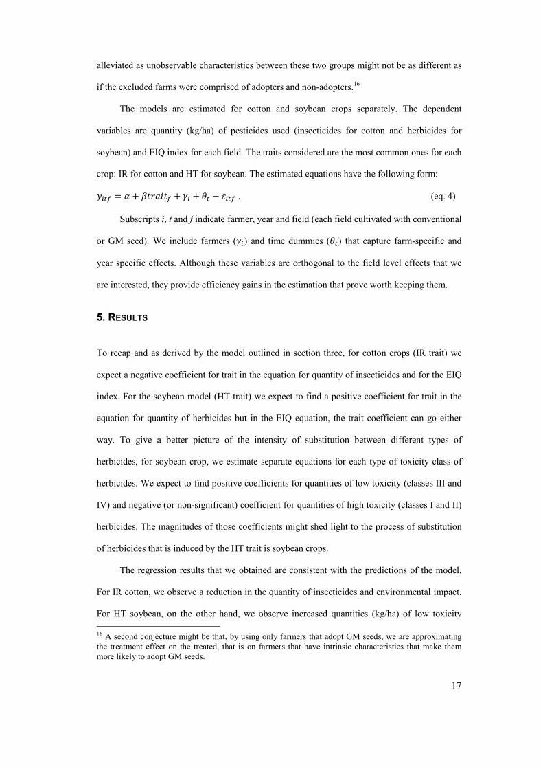
The models are estimated for cotton and soybean crops separately. The dependent

variables are quantity (kg/ha) of pesticides used (insecticides for cotton and herbicides for

soybean) and EIQ index for each field. The traits considered are the most common ones for each

crop: IR for cotton and HT for soybean. The estimated equations have the following form:

���� = � + ������� + �� + �� + ���� . (eq. 4)

Subscripts i, t and f indicate farmer, year and field (each field cultivated with conventional

or GM seed). We include farmers (��) and time dummies (��) that capture farm-specific and

year specific effects. Although these variables are orthogonal to the field level effects that we

are interested, they provide efficiency gains in the estimation that prove worth keeping them.

5. RESULTS

To recap and as derived by the model outlined in section three, for cotton crops (IR trait) we

expect a negative coefficient for trait in the equation for quantity of insecticides and for the EIQ

index. For the soybean model (HT trait) we expect to find a positive coefficient for trait in the

equation for quantity of herbicides but in the EIQ equation, the trait coefficient can go either

way. To give a better picture of the intensity of substitution between different types of

herbicides, for soybean crop, we estimate separate equations for each type of toxicity class of

herbicides. We expect to find positive coefficients for quantities of low toxicity (classes III and

IV) and negative (or non-significant) coefficient for quantities of high toxicity (classes I and II)

herbicides. The magnitudes of those coefficients might shed light to the process of substitution

of herbicides that is induced by the HT trait is soybean crops.

The regression results that we obtained are consistent with the predictions of the model.

For IR cotton, we observe a reduction in the quantity of insecticides and environmental impact.

For HT soybean, on the other hand, we observe increased quantities (kg/ha) of low toxicity

16 A second conjecture might be that, by using only farmers that adopt GM seeds, we are approximating the treatment effect on the treated, that is on farmers that have intrinsic characteristics that make them more likely to adopt GM seeds.

18

herbicides and no corresponding reduction for high toxicity ones. The net result is an increase in

EIQ index of herbicides applied.

Insect Resistant Cotton

Table 8 shows estimates of the effect of adoption of IR trait in cotton crops for quantities

(Kg/ha) of active ingredients of insecticides and total pesticides applied, considering all farms in

the survey and the restricted sample respectively. The point estimates in the restricted sample

are lower (in absolute terms) than the ones in the full sample, which indicates that bias due to

uncontrolled unobserved variables is an issue. The coefficient of the IR trait indicates that it

allows a reduction of 0.956Kg/ha of active ingredients of insecticides. Table 9 shows the results

estimated with farm and year fixed effects, which shows efficiency gains reflected in lower

standard errors obtained, and a log-linear specification that estimates the proportional effect of

adoption on the dependent variable. The result shows a decrease of 24% in the amount of

insecticides17 used and 9.2% in total quantity of active ingredients.

Table 10 is the counterpart of table 9 for the EIQ index. Consistent with the reduction in

quantity of insecticides, the coefficient indicates a reduction of 34.225 EIQ points. To gain

some perspective on this magnitude, in comparison with the general classification of active

ingredients for insecticides, this is higher than the median EIQ index of 32.07. Also, the Mean

EIQ for insecticides is 145.8 and for all pesticides 304.4. The log-linear specification shows a

proportional reduction of 23.4% in the EIQ index for insecticides. Hence, it can be considered a

significant reduction in terms of environmental index.

As a robustness check for our results, we perform a falsification test that consists on

regressing quantities (Kg/ha) of pesticides that should not be affected by the introduction of IR

trait: acaricides, fungicides and herbicides. Table 11 shows the results using all cotton farms and

the restricted sample and it can be seen that none of the coefficients are statistically significant.

The results so far are all consistent with the current state of the literature on

environmental effects of IR seeds. Studying IR cotton seeds in India, Qaim & Zilberman (2003)

17 We also estimate similar models per toxicity class (I-IV in decreasing level of toxicity) which indicate reductions in all classes, the most prominent effect being for class III (medium-low level of toxicity) with a proportional decrease of 40%. Those results are available upon request.

19

found reduction of 1 kg/ha on average use of insecticides (70% compared with the baseline

conventional field) while Qaim & de Janvry(2005) found reductions between 1.2kg/ha and

2.6Kg/ha of active ingredients used in Argentina, which represents about 50% reduction in

comparison with conventional plots. For China, Huan et al. (2005) found even bigger reductions

of about 49kg/ha of average insecticide use (80.5% compared to the average of 60.7 Kg/ha in

conventional fields).

Herbicide Tolerant Soybeans

For soybeans, the regression estimates on table 12 show that adoption of HT trait

increases the quantities (Kg/ha) of active ingredients of herbicides used. The point estimate for

the coefficient of the HT trait effect on the use of herbicides in the restricted sample is bigger

than the one in the full sample and indicates that it causes an increase of 0.996Kg/ha of active

ingredients of herbicides Table 13 shows the results including year and farmer fixed effects,

which provide efficiency gains in the estimation and a log-linear specification that shows a

proportionate increase of 44.2% in the quantity of active ingredients of herbicides and 26.2% in

total.

Table 14 breaks the effects on herbicides by categories of toxicity level (1 to 4 in

decreasing order). Categories 3 and 4 show significant increases of 0.64 and 0.44 kg/ha of active

ingredients respectively while categories 1 and 2 show reductions of 0.084 and 0.005 (not

statistically significant) respectively. Hence, the increases in less toxic herbicides is twelve fold

the reduction in more toxic herbicides. This result reflects two points on the pattern of herbicide

use. First, the substitution effect among different toxicity classes is very low, which indicates

that this channel of environmental benefits is very limited. Second, the scale effect is not so big

as compared to the effect found in other countries. Nevertheless, these results show that farmers

are increasing the use less toxic herbicides on top of the more toxic ones, which suggests more

environmental impact as a result of adoption of HT seeds.

The environmental effect is shown in Table 15 that reports the results for HT trait

coefficient on the EIQ index equation. The weakness of the substitution among herbicides of

20

different toxicity categories is reflected in higher environmental impact as shown by the

coefficient that indicates an increase of 13.847 EIQ points. In comparison with the general EIQ

classification for herbicides, this is lower than the median value for EIQ index of 19.5. The EIQ

for glyphosate is also larger than this result: 15.33. In the sample, the mean EIQ for herbicides

is 37.8 and for all pesticides 91.3. The proportional effect on the EIQ index is shows an increase

of 35.6% in the EIQ index for herbicides and 16.2% in total. Hence, we can conclude for a

relatively modest increase in environmental impact caused by HT soybeans.

We conduct two robustness checks for our results on HT soybeans. First, as with the case

of IR cotton, we run a falsification test that consists on regressing quantities (Kg/ha) of

pesticides that should not be affected by the introduction of HT trait: fungicides and

insecticides. Table 16 shows the results using all soybean farms and the restricted sample and it

can be seen that none of the coefficients are statistically significant. Additionally, we estimate

the models for quantities and environmental impact controlling for the use of no-tillage

cultivation in each field. This cultivation method requires more herbicides since it doesn’t use

tillage to clean the soil from weed infestation before the planting. Since this variable varies

between fields, it might capture an important characteristic that should be controlled for. Tables

17 and 18 show the results for quantity of active ingredients and environmental impact,

respectively, that are qualitatively and quantitatively very similar to the ones obtained before.

The results suggest that previous findings on the environmental effects of HT soybeans

might have been biased by the qualitative nature of the mix of herbicides. Fernandez-Cornejo et

al. (2002) found evidence of reduction in the use of acetamide herbicides and increase in the use

of glyphosate in USA. Qaim and Traxler (2005) studying HT seeds in Argentina found a total

increase of 107% in the use of herbicides, which are divided in a decreases of 87% and 100% in

toxicity classes two and three, respectively, and an increase of 248% in toxicity class four. The

authors suggest that this change is basically due to the use of no-till farming by adopters of HT

soybeans.

Our results are not incompatible with those previous findings. In fact, we also observe a

change in the composition of the mix of herbicides used towards less toxic products. This

21

movement is predicted by the theoretical analysis that shows how the HT trait increases the

value of marginal product of herbicide (glyphosate) and, therefore, the optimal amount used. On

the other hand, we also find very weak substitution among herbicides of different toxicity

classes, which suggests that the environmental impact of herbicides in being magnified. The

analysis with the EIQ index confirms that this is not only a possibility: even inducing more use

of a less toxic herbicide, HT seeds cause higher environmental impact, even when controlling

for the use of no-till farming.

6. CONCLUSION

In this paper we analyze the environmental effects related to the use of pesticides arising from

adoption of GM seeds in cotton and soybean crops. Cotton crops are genetically engineered to

display IR traits that make the plant produce a natural toxin that helps fight certain types of

harmful bollworms. Soybeans are modified to display HT trait that make the plant resistant to

glyphosate, a general purpose low toxicity herbicide. We use a model of profit maximizing

competitive farm to show how the introduction of these traits affects the optimal choices of

pesticides. We show that the IR trait works as a substitute for insecticides and reduces the

quantity used whereas the HT trait works as a complement for the herbicide glyphosate and so

induces more usage of this product.

The environmental effects are also different for each type of trait. The IR trait has

unequivocal benefits since it’s basically a chemical saving technology. The HT trait, on the

other hand, has ambiguous effects: it induces more usage of a less toxic herbicide but we argue

that the total effect depends on the substitution among herbicides of different toxicity classes

and on the scale of additional usage of glyphosate. Increased environmental impact can arise

from a combination of low substitution and high scale effect.

Using within-farm variation across fields treated with conventional and GM seeds, we

find that the IR trait reduces the amount of insecticides applied to cotton crops, measured by

kg/ha of active ingredients applied to the fields. HT trait, on the other hand, leads to more usage

of herbicides. Specifically, we see increased usage of herbicides from lower toxicity classes (3

22

and 4) and very small reductions in herbicides from higher toxicity classes (1 and 2). This

finding evidences a very weak substitution among herbicides which raises the possibility of

higher environmental impact.

To assess the environmental effect of GM traits due to the use of pesticides, we use a

measure developed by integrated pest management scientists that takes into account levels of

toxicity of active ingredients, risk of exposure and application in the field (dose and number of

applications): the EIQ index. Within-farm analysis shows that IR trait reduces the

environmental impact by about 23% in the treated fields compared to fields cultivated with

conventional seeds. This is consistent with the previous result on kg/ha of insecticides and

confirms the environmental impact saving nature of the IR technology.

The resulting environmental impact for HT trait, on the other hand, is found to be

positive. The estimates imply an increase of 35.6% on the impact of herbicides compared to

fields cultivated with conventional seeds. This finding confirms that the weak substitution

among herbicides makes adoption of HT seeds to increase the environmental impact from

pesticide use.

We believe this to be an important result for three reasons. First, it contributes to uncover

environmental effects that have been hidden by the qualitative nature of the mix of herbicides

induced by HT trait. Second, environmental policy makers designing policies for biotechnology

adoption might consider this new evidence to differentiate among GM traits that produce

positive or negative externalities. Finally, as the composition of the EIQ index suggests, the

environmental impact of pesticides can have multiple dimensions that might involve

farmworker health and safety, consumer safety and ecological impacts. Hence, the results on HT

soybeans points to additional avenues of work that should be taken to evaluate each of these

possible channels since they can also affect other important outcomes such as human capital

accumulation.

REFERENCES

Ameden, H., Qaim, M., & Zilberman, D. (2005). Adoption of Biotechnology in Developing Countries. In J. Cooper, L. Lipper, & D. Zilberman, Agricultural

23

Biodiversity and Biotechnology in Economic Development (pp. 329-357). New York: Springer.

Bidraban, P., Franke, A., Ferraro, D., Ghersa, C., Lotz, L., Nepomuceno, A., . . . van de Wiel, C. (2009). GM-related sustainability: agro-ecological impacts, risks and opportunities of soy production in Argentina and Brazil. Wageningen: Plant Research International B.V.

Brookes, G., & Barfoot, P. (2012). GM Crops: Global Socioeconomic and Environmental Inpacts 1996 - 2010. Dorchester: P.G. Economics.

Carpenter, J., & Gianessi, L. (1999). Herbicide Tolerant Soybeans: Why Growers are Adopting Roundup Ready Varieties. AgBioforum, 2(2), 65-72.

Céleres. (2012). The Economic Benefits from Crop Biotechnology in Brazil: 1996 - 2011. Report prepared for the Brazilian Association of Seeds Producers (ABRASEM), Uberlândia (MG). Retrieved June 2012, from http://www.cib.org.br/estudos/Rel_BiotechBenefits_2009_Economico_Eng.pdf

Crost, B., & Shankar, B. (2008). Bt-Cotton and Production Risk: Panel Data Estimates. International Journal of Biotechnology, 10, 122-131.

Fernandez-Cornejo, J., Klotz-Ingram, C., & Jans, S. (2002). Farm-level effects of adopting herbicide-tolerant soybeans in the U.S.A. Journal of Agricultural and Applied Economics, 149-163.

Huang, J., Hu, R., Rozelle, S., Qiao, F., & Pray, C. (2002). Transgenic Varieties and Productivity of Small-Holder Cotton Farmers in China. The Australian Journal of Agricultural and Resource Economics, 46, 367 - 387.

James, C. (2008). Global Status of commercialized Biothech/GM Crops: 2008. Int. Serv. Acquis. Agri-Biothech Appl., ISAAA, Ithaca, NY.

Kovach, J., Petzoldt, C., Degnil, J., & Tette, J. (1992). A method to measure the environmental impact of pesticides. Ithaca, NY: New York State Agricultural Experiment Station, a division of the New York State College of Agriculture and Life Sciences, Cornell University.

Levitan, J., Merwin, I., & Kovach, J. (1995). Assessing the Relative Environmental Impacts of Agricultural Pesticides: the Quest for a Holistic Method. Agriculture, Ecosystems and Environment, 55, 153-168.

Lichtenberg, E., & Zilberman, D. (1986). The Econometrics of Damage Control: Why Specification Matters. American Journal of Agricultural Economics, 68(3), 261 - 273.

Oliveira, A., Silveira, J., & Alvim, A. (2012, March). Cartagena Protocol, Biosafety and Grain Segregation: The Effects on the Soybean Logistics in Brazil. Jounal of Agricultural Research and Developmento, 2(1), 17-30.

Pelaez, V. (2009). State of Exception in the Regulation of Genetically Modified Organisms in Brazil. Science and Public Policy, 36(1), 61 - 71.

Qaim, M. (2009). The Economics of Genetically Modified Crops. Annual Review of Resource Economics, 1, 665 - 694. Retrieved from http://www.annualreviews.org/doi/abs/10.1146/annurev.resource.050708.144203

Qaim, M., & de Janvry, A. (2005). Bt Cotton and Pesticide use in Argentina: Economic and Environmental Effects. Environment and Development Economics, 10, 179 - 200.

Qaim, M., & Traxler, G. (2005). Roundup Ready soybeans in Argentina: farm level and aggregate welfare effects. Agricultural Economics, 73-86.

Qaim, M., & Zilberman, D. (2003). Yield Effects of Genetically Modified Crops in Developing Countries. Science, 299(5608), 900 - 902.

24

Sexton, S., & Zilberman, D. (2012). Land for Food and Fuel Production: The Role of Agricultural Biotechnology. In J. Zivin , & J. Perloff, The Intended and Unintended Effects of U.S. Agricultural and Biotechnology Policies (pp. 269 - 288). Chicago: University of Chicago Press.

Sharma, D. (2004). Food and Hunger: a View from the South. Forum on Biotechnology and Food Security. New Delhi.

United States Environmental Protection Agency. (1993). Registration Decision Fact Sheet for Glyphosate (EPA-738-F-93-011). Retrieved 11 02, 2013, from http://www.epa.gov/oppsrrd1/REDs/factsheets/0178fact.pdf

Weihold, D., Killick, E., & Reis, E. (2013). Soybeans, Poverty and Inequality in the Brazilian Amazon. World Development, 52, 132-143.

25

Tables and Figures Figure 1: Steady Increase in Global Planted Area Using GM Crops

Source: Qaim (2009). Figure 2: Share of Planted Area with Genetically Modified Seeds for Cotton, Maize and Soybeans (2008-2011)

Source: own elaboration based on Celeres (2012)

0.0%

10.0%

20.0%

30.0%

40.0%

50.0%

60.0%

70.0%

80.0%

90.0%

100.0%

2008 2009 2010 2011

6.6%11.2%

35.9%29.6%

0.0%

23.2%

60.1%

79.2%

45.2%

60.3%

76.9%

91.8%

Cotton Maize Soybeans

26

Left panel: IR trait reduces the value of marginal product of insecticides (from VMP0 to VMP1) due to compound effect over insects and so reduces the optimal quantity of insecticides (from ��

∗ to ��∗).

Right panel: HT trait increases the value of marginal product of herbicide (from ���� to ����) due to reduction of harmful side-effects and so increases the optimal quantity of herbicide (from ��

∗ to ��∗).

Figure 4: EIQ Components

EIQ for active ingredient: average of ecological, consumer and farmworker components:

• ���������� = (� × �) + �� ×���

�× 3� + (� × � × 3) + (� × � × 5), F = fish toxicity, R =

surface runoff potential, D = bird toxicity, S = soil half-life, P = plant surface half-life, D = bird toxicity, Z = bee toxicity and B = beneficial arthropod toxicity;

• �������� = � × ����

�� × �� + �, C = chronical toxicity, SY = systemicity (potential of

absorption, by plant) L = leaching potential, S = soil half-life and P = plant surface half-life • ���������� = � × [(�� × 5) + (�� × �)], C = chronical toxicity, P = plant surface half-life

and DT = dermal toxicity.

EIQ

Ecological Component

Terrestrial Effects

Beneficial Arthropod

Bees

Bird

Aquatic Effects

Fish

Surface Loss

Consumer Component

Consumer

Chronic Toxicity

Systemicity

Soil Half-life, plant surface and

half-life

Groundwater

Leaching potential

Farmworker Component

Picker Effect

Chronic toxicity

Acute toxicity

Plant surface half-life

Applicator

Chronic toxicity

Acute toxicity

Figure 3: Effect of GM Traits on Pesticide Use

VMP1 VMP0

��∗ ��

∗

w

VMP0 VMP1

��∗ ��

∗

w

x x

IR trait HT trait

27

Figure 5: Cities with Cotton Farms Surveyed

28

Figure 6: Cities with Soybean Farms Surveyed

Table 1: Distribution of Cotton and Soybean Farms by Region

Cotton Soybean Region N pct. N pct. Central-West 145 67.44 124 48.06 Northeast 62 28.84 25 9.69 South - - 95 36.82 Southeast 8 3.72 14 5.43 Total 215 100.00 258 100.00 Note: farms are spread over 8 states (figs. 5 and 6) which comprise a total area of 3,564.8 thousands Km2, equivalent to 41.8% of Brazilian territory.

29

Table 2: Farm-Level Descriptive Statistics for Cotton Growers

mean sd min max count Planted Area (ha) 2,521.0 3,538.5 60.0 28,374.0 255 Net Rev. (US$/ha) 3,344.1 1,364.9 791.6 7,171.2 255 Gross Margin (US$/ha) 1,495.5 1,112.4 -6.2 4.988.8 255 Costs (US$/ha) 1,848.6 412.0 604.6 2,586.7 255 Pesticides (US$/ha) 588.2 194.9 99.9 1,144.9 255 Fertilizers (US$/ha) 1,007.2 270.7 304.5 1,927.5 255 Central-West 0.67 0.47 0.0 1.0 215 Northeast 0.29 0.45 0.0 1.0 215 South 0.00 0.00 0.0 0.0 215 Southeast 0.04 0.19 0.0 1.0 215 Basic School 0.07 0.26 0.0 1.0 83 High School 0.29 0.46 0.0 1.0 83 College 0.53 0.50 0.0 1.0 83 Graduate Degree 0.11 0.31 0.0 1.0 83 Age 38.08 9.14 23.0 57.0 75 Experience 25.80 14.60 2.0 58.0 75 Owner 0.02 0.15 0.0 1.0 215 Biotech User 0.43 0.50 0.0 1.0 215 IR user 0.26 0.44 0.0 1.0 255 Sample: 2009 – 2011. Area, revenue, expenditures and IR trait use statistics consider each farm/year as a separate observation since they can change over the years for farms that are surveyed more than once. Other statistics consider each farm as a separate observation and are not influenced by farms that appear in more than one survey. Age and experience correspond to the maximum value of that variable observed. “Biotech User” shows whether the farmer adopted any type of GM seed over the surveyed years. The value is different than “IR user” since there are other types of GM seeds for cotton.

30

Table 3 Farm-Level Descriptive Statistics for Soybean Growers

mean sd min max count Planted Area (ha) 1,240.3 1,771.8 8.0 13,500.0 291 Net Rev. (US$/ha) 1,164.8 484.9 334.3 3,711.6 291 Gross Margin (US$/ha) 499.3 352.7 -140.4 2,115.5 291 Costs (US$/ha) 665.6 248.2 283.6 1998.2 291 Pesticides (US$/ha) 135.5 86.8 17.0 630.1 291 Fertilizers (US$/ha) 478.3 190.2 0.0 1,383.4 291 Central-West 0.48 0.50 0.0 1.0 258 Northeast 0.10 0.30 0.0 1.0 258 South 0.37 0.48 0.0 1.0 258 Southeast 0.05 0.23 0.0 1.0 258 Basic School 0.28 0.45 0.0 1.0 120 High School 0.27 0.44 0.0 1.0 120 College 0.38 0.49 0.0 1.0 120 Graduate Degree 0.08 0.28 0.0 1.0 120 Age 43.97 12.41 24.0 74.0 118 Experience 32.46 17.10 5.0 75.0 118 Owner 0.22 0.42 0.0 1.0 258 HT User 1.00 0.06 0.0 1.0 258 Sample: 2009 – 2011. Area and expenditure statistics consider each farm/year as a separate observation since they can change over the years for farms that are surveyed more than once. Other statistics consider each farm as a separate observation and are not influenced by farms that appear in more than one survey. Age and experience correspond to the maximum value of that variable observed. “HT User” shows whether the farmer adopted HT seeds over the surveyed years. Since HT is the only GM seed for soybean, this table doesn’t display a variable “Biotech User”.

Table 4: Within-Farm Descriptive Statistics: Fields Cultivated with Conventional vs. Fields Cultivated with Insect Resistant Cotton

CO IR Total Diff. Area (ha) 1,741.9 1,087.2 1,414.6 654.7 [2,442.4] [1,948.8] [2,224.5] [1.62] Yield (Kg/ha) 3,871.8 3,560.2 3,716.0 311.6 [521.9] [1,120.3] [884.2] [1.95] Net Rev. (US$/ha) 5,980.2 6,077.3 6,027.5 -97.08 [2,253.7] [2,273.0] [2,253.9] [-0.23] Direct Costs (US$/ha) 3,563.3 3,533.3 3,548.7 30.03 [433.0] [480.6] [455.1] [0.36] Costs-Seed (US$/ha) 3,461.8 3,349.3 3,407.0 112.5 [440.1] [474.8] [458.8] [1.33] Gross Margin (US$/ha) 2,416.9 2,544.0 2,478.8 -127.1 [2156.2] [2178.2] [2158.5] [-0.32] Fertilizers (US$/ha) 992.1 981.4 986.9 10.63 [214.9] [219.7] [216.4] [0.26] Observations 60 60 120 60 Standard errors (columns CO and IR) and t statistics (column Diff.) in brackets. * p < 0.05, ** p < 0.01, *** p < 0.001 Cost-Seed: excludes expenditures with seeds and royalties.

31

Table 5: Within-Farm Descriptive Statistics: Fields Cultivated with Conventional vs. Fields Cultivated with Herbicide Tolerant Soybean

CO HT Total Diff. Area (ha) 692.6 706.6 699.6 -14.01 [992.0] [773.2] [886.7] [-0.10] Yield (Kg/ha) 3,148.1 3,146.8 3,147.5 1.240 [512.9] [603.6] [558.4] [0.01] Net Rev. (US$/ha) 1,865.3 1,850.9 1,858.0 14.42 [390.8] [419.2] [404.2] [0.23] Direct Costs (US$/ha) 1,180.3 1,193.3 1,186.8 -12.92 [241.4] [247.4] [243.8] [-0.34] Costs-Seed (US$/ha) 1,085.4 1,066.8 1,076.1 18.62 [243.3] [249.6] [245.9] [0.49] Gross Margin (US$/ha) 685.0 657.6 671.2 27.34 [439.7] [442.3] [439.9] [0.40] Fertilizers (US$/ha) 489.0 488.0 488.5 0.936 [180.3] [179.1] [179.2] [0.03] 85 85 170 85 Standard errors (columns CO and HT) and t statistics (column Diff.) in brackets. * p < 0.05, ** p < 0.01, *** p < 0.001 Cost-Seed: excludes expenditures with seeds and royalties.

32

Table 6: Differences Between Cotton Farms Included (Sample) and not Included (Non-Sample) in Regression Analysis

Non-Sample Sample Total Diff. Total Area (ha) 2,371.5 3,006.6 2,521.0 -635.1 [3,273.7] [4,284.0] [3,538.5] [-1.06] Net Rev. (US$/ha) 3,403.3 3,151.7 3,344.1 251.6 [1,323.3] [1,487.7] [1,364.9] [1.17] Gross Margin (US$/ha) 1,547.6 1,326.2 1,495.5 221.4 [1051.1] [1,286.9] [1,112.4] [1.21] Costs (US$/ha) 1,855.7 1,825.5 1,848.6 30.25 [429.7] [350.7] [412.0] [0.55] Pesticides (US$/ha) 592.1 575.5 588.2 16.55 [205.5] [156.0] [194.9] [0.66] Fertilizers (US$/ha) 1,001.8 1,024.7 1,007.2 -22.91 [279.9] [239.9] [270.7] [-0.62] Age 38.24 34.76 37.28 3.478 [9.165] [10.44] [9.611] [1.58] Experience 23.70 19.03 22.41 4.663 [15.93] [10.93] [14.82] [1.71] Owner 0.0103 0.0667 0.0235 -0.0564 [0.101] [0.252] [0.152] [-1.70] Central-West 0.749 0.317 0.647 0.432*** [0.435] [0.469] [0.479] [6.34] Northeast 0.241 0.567 0.318 -0.326*** [0.429] [0.500] [0.466] [-4.56] Southeast 0.0103 0.117 0.0353 -0.106* [0.101] [0.324] [0.185] [-2.51] Basic School 0.0595 0.0313 0.0517 0.0283 [0.238] [0.177] [0.222] [0.70] High School 0.321 0.125 0.267 0.196* [0.470] [0.336] [0.444] [2.50] College 0.571 0.594 0.578 -0.0223 [0.498] [0.499] [0.496] [-0.22] Graduate Degree 0.0476 0.250 0.103 -0.202* [0.214] [0.440] [0.306] [-2.49] Sample: farms that use both conventional and IR seeds and so are included in regression analysis. Non-Sample: farms that use only one type of seed (conventional or IR) and are not included in regression analysis. Total: all farms. Standard errors (columns Non-Sample, Sample and Total) and t statistics (column Diff.) in brackets. * p < 0.05, ** p < 0.01, *** p < 0.001

33

Table 7: Differences Between Soybean Farms Included (Sample) and not Included (Non-Sample) in Regression Analysis

Non-Sample Sample Total Diff. Total Area (ha) 868.2 2,142.3 1,240.3 -1,274.1*** [1,201.7] [2,480.1] [1,771.8] [-4.52] Net Rev. (US$/ha) 1,160.5 1,175.5 1,164.8 -14.99 [415.2] [625.2] [484.9] [-0.20] Gross Margin (US$/ha) 530.1 424.5 499.3 105.6* [344.6] [362.8] [352.7] [2.29] Costs (US$/ha) 630.4 750.9 665.6 -120.6** [192.3] [334.8] [248.2] [-3.12] Pesticides (US$/ha) 122.9 166.2 135.5 -43.38** [64.33] [120.6] [86.76] [-3.14] Fertilizers (US$/ha) 443.8 561.9 478.3 -118.1*** [159.7] [229.5] [190.2] [-4.33] Age 46.55 38.94 43.98 7.613*** [11.06] [12.65] [12.13] [3.57] Experience 34.20 20.08 29.43 14.12*** [15.53] [13.80] [16.35] [5.58] Owner 0.248 0.271 0.254 -0.0230 [0.433] [0.447] [0.436] [-0.40] Central-West 0.466 0.518 0.481 -0.0516 [0.500] [0.503] [0.501] [-0.80] Northeast 0.0291 0.235 0.0893 -0.206*** [0.169] [0.427] [0.286] [-4.32] South 0.490 0.118 0.381 0.373*** [0.501] [0.324] [0.487] [7.52] Southeast 0.0146 0.129 0.0481 -0.115** [0.120] [0.338] [0.214] [-3.06] Basic School 0.367 0.0612 0.265 0.306*** [0.485] [0.242] [0.443] [5.11] High School 0.235 0.306 0.259 -0.0714 [0.426] [0.466] [0.439] [-0.90] College 0.337 0.469 0.381 -0.133 [0.475] [0.504] [0.487] [-1.53] Graduate Degree 0.0612 0.163 0.0952 -0.102 [0.241] [0.373] [0.295] [-1.74] Sample: farms that use both conventional and HT seeds and so are included in regression analysis. Non-Sample: farms that use only one type of seed (conventional or HT) and are not included in regression analysis. Total: all farms. Standard errors (columns Non-Sample, Sample and Total) and t statistics (column Diff.) in brackets. * p < 0.05, ** p < 0.01, *** p < 0.001

34

Table 8 OLS Estimates of Effects of IR Trait on Quantity of Insecticides and Total Pesticides Dependent Variable: Active Ingredients (Kg/ha)

(1) (2) (3) (4) Insecticides+ Total+ Insecticides Total IR trait -1.279*** -1.790*** -0.956** -0.980 [0.264] [0.485] [0.362] [0.568] Constant 4.914*** 12.352*** 4.630*** 11.551*** [0.163] [0.314] [0.256] [0.413] N 312 312 120 120 r2 0.046 0.025 0.056 0.025 F 11.141 145.516 12.215 8.340 Mean of Dep. Var. 4.639 11.967 4.152 11.061 Models (1) and (2) include all cotton farms, models (3) and (4) only farms that use both conventional and IR seeds (within farm variation as source of identification). Models are in linear specification. + Robust standard errors in brackets. * p < 0.05, ** p < 0.01, *** p < 0.001 IR trait affects the quantity (Kg/ha) of insecticides. Total represents the sum of all pesticides used (acaricides, fungicides, herbicides and insecticides). Coefficients are smaller in magnitude in the restricted sample, but not statistically different than the ones in the model with all farms.

Table 9 OLS Estimates of Effects of IR Trait on Quantity of Insecticides and Total Pesticides (Restricted Sample) Dependent Variable: Active Ingredients (Kg/ha)

(1) (2) (3) (4) Insecticides+ Total+ Insecticides Total IR trait -0.956*** -0.980*** -0.242*** -0.092*** [0.155] [0.252] [0.037] [0.024] Constant 8.721*** 19.018*** 2.346*** 3.025*** [0.874] [0.644] [0.207] [0.134] N 120 120 120 120 r2 0.905 0.896 0.913 0.878 F 11.141 145.516 12.215 8.340 Mean of Dep. Var. 4.152 11.061 - - Models (1) and (2) are linear specifications, models (3) and (4) are log-linear specifications. All models include farm and year fixed-effects. Restricted saple: farms that use both conventional and IR seeds (within farm variation as source of identification). + Robust standard errors in brackets. * p < 0.05, ** p < 0.01, *** p < 0.001 Farmer and year fixed-effects don't affect coefficients since they are orthogonal to within-farm variables. Log-linear specifications show a reduction of 24% in the quantity of insecticides and 9.2% in total pesticides.

35

Table 10 OLS Estimates of Environmental Impact of IR Trait (Restricted Sample) Dependent Variable: EIQ

(1) (2) (3) (4) Insecticides+ Total+ Insecticides+ Total+ IR trait -34.225*** -36.856*** -0.234*** -0.120*** [5.525] [7.482] [0.035] [0.026] Constant 316.085*** 557.297*** 6.041*** 6.455*** [23.144] [42.071] [0.198] [0.082] N 120 120 120 120 r2 0.906 0.905 0.918 0.886 F 48.981 11.134 12.972 75.140 Mean of Dep. Var. 145.807 304.489 - - Models (1) and (2) are linear specifications, models (3) and (4) are log-linear specifications. All models include farm and year fixed-effects. Restricted saple: farms that use both conventional and IR seeds (within farm variation as source of identification). + Robust standard errors in brackets. * p < 0.05, ** p < 0.01, *** p < 0.001 Consistent with the reduction in quantity of insecticides, the coefficient indicates a reduction of 34.225 EIQ points. In comparison with the general classification of active ingredients for insecticides, this is higher than the median EIQ index of 32.07. The log-linear specification shows a proportional reduction of 23.4% in the EIQ index.

Table 11 Robustness Check: OLS Estimates of Effect of IR Trait on Other Pesticides. Dependent Variable: Active Ingredients (Kg/ha).

(1) (2) (3) (4) (5) (6) Acaricides Fungicides Herbicides Acaricides Fungicides Herbicides IR trait 0.003 -0.063 -0.346 -0.011 0.007 -0.056 [0.049] [0.091] [0.366] [0.027] [0.032] [0.191] Constant 0.428*** 0.956*** 4.933*** 0.544*** 1.283*** 7.723*** [0.023] [0.042] [0.170] [0.152] [0.181] [1.075] N 312 312 312 120 120 120 r2 0.000 0.002 0.003 0.906 0.950 0.840 F 0.003 0.481 0.894 11.185 22.264 6.123 Mean of Dep. Var.

0.429 0.942 4.858 0.455 0.869 4.608

Models (1)-(3) include all farms and models (4)-(6) only restricted sample (farms that use conventional and IR seeds) with farm and year fixed-effects. All models are linear specifications. + Robust standard errors in brackets. * p < 0.05, ** p < 0.01, *** p < 0.001 Falsification test shows that other pesticides are not affected by IR trait.

36

Table 12 OLS Estimates of Effects of HT Trait on Quantity of Herbicides and Total Pesticides Dependent Variable: Active Ingredients (Kg/ha)

(1) (2) (3) (4) Herbicides+ Total+ Herbicides+ Total+ HT Trait 0.762*** 0.546*** 0.996*** 0.995*** [0.099] [0.150] [0.138] [0.202] Constant 1.741*** 3.284*** 1.769*** 3.315*** [0.075] [0.121] [0.074] [0.122] N 376 376 170 170 r2 0.091 0.025 0.236 0.126 F 59.114 13.192 51.766 24.194 Mean of Dep. Var. 2.326 3.703 2.267 3.813 Models (1) and (2) include all soybean farms, models (3) and (4) only farms that use both conventional and HT seeds (within farm variation as source of identification). Models are in linear specification. + Robust standard errors in brackets. * p < 0.05, ** p < 0.01, *** p < 0.001 HT trait affects the quantity (Kg/ha) of herbicides. Total represents the sum of all pesticides used (fungicides and insecticides).

Table 13 OLS Estimates of Effects of HT Trait on Quantity of Herbicides and Total Pesticides (Restricted Sample) Dependent Variable: Active Ingredients (Kg/ha)

(1) (2) (3) (4) Herbicides+ Total+ Herbicides Total HT Trait 0.996*** 0.995*** 0.442*** 0.262*** [0.089] [0.096] [0.056] [0.027] Constant 4.518*** 5.930*** 2.206*** 1.848*** [0.880] [0.814] [0.486] [0.214] N 170 170 170 170 r2 0.836 0.899 0.755 0.888 F 90.919 249.438 3.278 144.793 Mean of Dep. Var. 2.267 3.813 - - Models (1) and (2) are linear specifications, models (3) and (4) are log-linear specifications. All models include farm and year fixed-effects. Restricted saple: farms that use both conventional and HT seeds (within farm variation as source of identification). + Robust standard errors in brackets. * p < 0.05, ** p < 0.01, *** p < 0.001 Farmer and year fixed-effects don't affect coefficients since they are orthogonal to within-farm variables. Log-linear specifications show as increase of 44.2% in the quantity of herbicides and 26.3% in total pesticides.

37

Table 14 OLS Estimates of Effects of HT Trait on Quantity of Herbicides per Toxicity Level (Restricted Sample) Dependent Variable: Active Ingredients (Kg/ha)

(1) (2) (3) (4) Herbicides 1 Herbicides 2 Herbicides 3 Herbicides 4 HT Trait -0.084*** -0.005 0.635*** 0.438*** [0.021] [0.054] [0.098] [0.090] Constant 0.444*** 0.053 2.103*** -0.499 [0.046] [0.344] [0.466] [0.523] N 168 168 168 168 r2 0.887 0.777 0.855 0.845 F 508.764 404.682 20.309 12.929 Mean of Dep. Var. 0.200 0.219 1.124 0.706 Restricted sample: farms that use both conventional and HT seeds (within farm variation as source of identification). Robust standard errors in brackets. * p < 0.05, ** p < 0.01, *** p < 0.001 Toxicity levels 1 - 4 in decreasing order (from more to less toxic). Herbicides based on Glyphosate are considered of lower toxicity level. Increases in less toxic herbicides (levels 3 and 4) are twelvefold the decreases in more toxic ones (levels 1 and 2).

Table 15 OLS Estimates of Environmental Impact of HT Trait (Restricted Sample) Dependent Variable: EIQ

(1) (2) (3) (4) Herbicides Total Herbicides Total HT Trait 13.847*** 14.329*** 0.356*** 0.162*** [1.639] [2.054] [0.049] [0.023] Constant 75.205*** 140.924*** 4.987*** 4.925*** [13.188] [12.379] [0.472] [0.136] N 170 170 170 170 r2 0.836 0.936 0.790 0.933 F 634.267 1378.593 142.869 556.876 Mean of Dep. Var. 37.875 91.337 - - Models (1) and (2) are linear specifications, models (3) and (4) are log-linear specifications. All models include farm and year fixed-effects. Restricted sample: farms that use both conventional and HT seeds (within farm variation as source of identification). Robust standard errors in brackets. * p < 0.05, ** p < 0.01, *** p < 0.001 Weakness of the substitution among herbicides of different toxicity categories is reflected in higher environmental impact as shown by the coefficient that indicates an increase of 13.847 EIQ points. Log-linear specifications show an increase of 35.6% in the EIQ index for herbicides and 16.2% in total. In comparison with the general EIQ classification for herbicides, this is lower than the median value for EIQ index of 19.5. The EIQ for glyphosate is also larger than this result: 15.33. Result can be interpreted as reflecting the weakness of substitution between high and low toxicity herbicides shown in table 14.

38

Table 16 Robustness Check: OLS Estimates of Effect of HT Trait on Other Pesticides Dependent Variable: Active Ingredients (Kg/ha)

(1) (2) (3) (4) Fungicides Insecticides Fungicides Insecticides HT Trait -0.047 -0.131* 0.021* -0.007 [0.047] [0.066] [0.009] [0.020] Constant 0.445*** 0.841*** 0.913*** -0.017 [0.042] [0.058] [0.045] [0.178] N 376 376 170 170 r2 0.003 0.011 0.989 0.970 F 0.975 3.955 1228.421 20622.927 Mean of Dep. Var. 0.409 0.740 0.454 0.840 Models (1)-(2) include all farms and models (3)-(4) only restricted sample (farms that use conventional and HT seeds) with farm and year fixed-effects. All models are linear specifications. Robust standard errors in brackets. * p < 0.05, ** p < 0.01, *** p < 0.001 Falsification test shows that other pesticides are not affected by HT trait.

Table 17 Robustness Check: OLS Estimates of Effects of HT Trait on Quantity of Herbicides and Total Pesticides and Controlling for No-Tillage Cultivation (Restricted Sample) Dependent Variable: Active Ingredients (Kg/ha)

(1) (2) (3) (4) Herbicides Total Herbicides Total HT Trait 0.983*** 0.983*** 0.892*** 0.876*** [0.089] [0.096] [0.089] [0.095] No Tillage 0.180 2.443*** [0.469] [0.469] Constant 2.272*** 3.095*** 1.038*** 4.069*** [0.328] [0.392] [0.096] [0.091] N 168 168 154 154 r2 0.833 0.899 0.829 0.887 F 248.083 363.742 864.663 4047.737 Mean of Dep. Var. 2.248 3.8 2.180 3.626 Restricted Sample: farms that use conventional and HT soybeans (within-farm variation as source of identification). All models use linear specifications and farm and year fixed-effects. Robust standard errors in brackets. * p < 0.05, ** p < 0.01, *** p < 0.001 Models (1) and (2) control for the use of no-tillage techniques that require more herbicides than conventional planting. Models (3) and (4) consider only farmers that use conventional planting.

39

Table 18 Robustness Check: OLS Estimates of Environmental Impact of HT Trait Controlling for No-Tillage Cultivation (Restricted Sample) Dependent Variable: EIQ

(1) (2) (3) (4) Herbicides Total Herbicides Total HT Trait 13.457*** 13.944*** 12.151*** 11.951*** [1.613] [2.043] [1.667] [2.047] No Tillage 3.160 69.325*** [6.713] [6.513] Constant 36.751*** 68.413*** 16.518*** 112.068*** [5.635] [9.850] [0.999] [1.119] N 168 168 154 154 r2 0.828 0.937 0.814 0.928 F 355.885 1213.411 308.650 1698.950 Mean of Dep. Var. 37.280 90.935 36.006 85.974 Restricted Sample: farms that use conventional and HT soybeans (within-farm variation as source of identification). All models use linear specifications and farm and year fixed-effects. Robust standard errors in brackets. * p < 0.05, ** p < 0.01, *** p < 0.001 Models (1) and (2) control for the use of no-tillage techniques that require more herbicides than conventional planting. Models (3) and (4) consider only farmers that use conventional planting.