Text Classification Chapter 2 of “Learning to Classify Text Using Support Vector Machines” by...

Text Classification

Chapter 2 of “Learning to Classify Text Using Support Vector Machines” by Thorsten Joachims, Kluwer, 2002.

Text Classification (TC) : Definition

• Infer a classification rule from a sample of labelled training documents (training set) so that it classifies new examples (test set) with high accuracy.

• Using the “ModApte” split, the ratio of training documents to test documents is 3:1

Three settings

• Binary setting (simplest). Only two classes, e.g. “relevant” and “non-relevant” in IR, “spam” vs. “legitimate” in spam filters.

• Multi-class setting, e.g. email routing at a service hotline to one out of ten customer representatives, Can be reduced into binary tasks: “one against the rest” strategy.

• Multi-label setting – e.g. semantic topic identifiers for indexing news articles. An article can be in one, many, or no categories. Can also be split into a set of binary classification tasks.

Representing text as example vectors

• The basic blocks for representing text will be called indexing terms

• Word-based are most common. Very effective in IR, even though words such as “bank” have more than one meaning.

• Advantage of simplicity – split the input text into words by white space.

• Assume the ordering of words is irrelevant – the “bag of words” model. Only the frequency of each word in the document is recorded.

• “bag of words” model ensures that each document is represented by a vector of fixed dimensionality. Each component of the vector represents the value (e.g. the frequency of that word in that document, TF) of one attribute.

Other levels of text representation

• More sophisticated representations than the “bag-of-words” have not yet shown consistent and substantial improvements

• Sub-word level, e.g. n-grams are robust against spelling errors. See Kjell’s neural network.

• Multi-word level. May use syntactic phrase indexing such as noun phrases (e.g. adjective-noun) followed by co-occurrence patterns (e.g. speed limit)

• Semantic level. Latent Semantic Indexing (LSI) aims to automatically generate semantic categories based on a bag of words representation. Another approach would make use of thesauri.

Feature Selection

• To remove irrelevant or inappropriate attributes from the representation.

• Advantages are protection against over-fitting, and increased computational efficiency with fewer dimensions to work with.

• 2 most common strategies:• a) Feature subset selection: use a subset of the

original features • b) Feature construction: new features are

introduced by combining original features.

Feature subset selection techniques

• Stopword elimination (removes high frequency words)

• Document frequency thresholding (remove infrequent words, e.g. those occurring less than m times in the training corpus)

• Mutual information• Chi-squared test (X²)• But: an appropriate learning algorithm should be

able to detect irrelevant features as part of the learning process.

Mutual Information

• We consider the association between a term t and a category c. How often do they occur together, compared with how common the term is, and how common is membership of the category?

• A is the number of times t occurs in c• B is the number of times t occurs outside c• C is the number of times t does not occur in c• D is the number of times t does not occur outside c• N = A + B + C + D. • MI(t,c) = log (A.N / ((A + C)(A + B)) )• If MI > 0 then there is a positive association between t and c• If MI = 0 there is no association between t and c• If MI < 0 then t and c are in complementary distribution• Units of MI are bits of information.

Chi-squared measure (X²)

• X²(t,c) = N.(AD-CB)² / (A+C).(B+D).(A+B).(C+D).• E.g. X² for words in US as opposed to UK English (1990s)• percent 485.2; U 383.3; toward 327.0; program 324.4;

Bush 319.1; Clinton 316.8; President 273.2; programs 262.0; American 224.9; S 222.0.

• These feature subset selection methods do not allow for dependencies between words, e.g. “click here”.

• See Yang and Pedersen (1997), A Comparative Study on Feature Selection in Text Categorisation.

Term Weighting

• A “soft” form of feature selection.• Does not remove attributes, but adjusts their relative

influence.• Three components:• Document component (e.g. binary, present in document =

1, absent = 0; term frequency (TF))• Collection component (e.g. inverse document frequency

log (N / DF))• Normalisation component, so that large and small

documents can be compared on the same scale e.g. 1 / sqrt(sum of xj²)

• The final weight is found by multiplying the 3 components

Feature Construction

• The new features should represent most of the information in the original representation while minimising the number of attributes.

• Examples of techniques are:• Stemming• Thesauri group words into semantic categories,

e.g. synonyms can be placed in equivalence classes.

• Latent Semantic Indexing• Term clustering

Learning Methods

• Naïve Bayes classifier

• Rocchio algorithm

• K-nearest neighbours

• Decision tree classifier

• Neural Nets

• Support Vector Machines

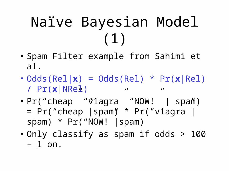
Naïve Bayesian model (2)

• Sahimi et al. use word indicators, and also the following non-word indicators:

• Phrases: free money, only $, over 21• Punctuation: !!!!• Domain name of sender: .edu less likely to be

spam than .com• Junk mail more likely to be sent at night than

legitimate mail.• Is recipient an individual user or a mailing list?

Our Work on the Enron Corpus- The PERC (George Ke)

Find a centroid ci for each category Ci

For each test document x:

Find k nearest neighbouring training documents to x

Similarity between x and the training document dj is added to similarity between x and ci

Sort similarity scores sim(x,Ci) in descending order

Decision to assign x to Ci can be made using various thresholding strategies

Rationale for the PERC Hybrid Approach

• Centroid method overcomes data sparseness: emails tend to be short.

• kNN allows the topic of a folder to drift over time. Considering the vector space locally allows matching against features which are currently dominant.

Kjell: A Stylometric Multi-Layer Perceptron

aa

ab

ac

ad

ae

h1

h2

h3

o1

o2

(Shakespeare)

(Marlowe)

input layer

“hidden” layer

output layer

w11

Performance Measures (PM)

• PM used for evaluating TC are often different from those optimised by the learning algorithms.

• Loss-based measures (error rate and cost models).

• Precision and recall-based measures.

Error Rate and Asymmetric Cost

• Error Rate is defined as the probability of the classification rule predicting the wrong class,

• Err = (f+- + f-+) / (f++ + f+- + f-+ + f--)• Problem: negative examples tend to outnumber positive

examples. So if we always guess “not in category”, it seems that we have a very low error rate.

• For many applications, predicting a positive example correctly is of higher utility than predicting a negative example correctly.

• We can incorporate this into the performance measure using a cost (or inversely, utility) matrix:

• Err = (C++f++ + C+-f+- + C-+f-+ + C--f--) / (f++ + f+- + f-+ + f--)

Precision and Recall

• The Recall of a classification rule is the probability that a document that should be in the category is classified correctly

• R = f++ / (f++ + f-+) • Precision is the probability that a document

classified into a category is indeed classified correctly

• P = f++ / (f++ + f+-)• F = 2PR / (P + R) if P and R are equally important

Micro- and macro- averaging

• Often it is useful to compute the average performance of a learning algorithm over multiple training/test sets or multiple classification tasks.

• In particular for the multi-label setting, one is usually interested in how well all the labels can be predicted, not only a single one.

• This leads to the question of how the results of m binary tasks can be averaged to get a single performance value.

• Macro-averaging: the performance measure (e.g. R or P) is computed separately for each of the m experiments. The average is computed as the arithmetic mean of the measure over all experiments

• Micro-averaging: instead average the contingency tables found for each of m experiments, to produce f++(ave), f+-(ave), f-+(ave), f--(ave). For recall, this implies

• R(micro) = f++(ave) / (f++ + f-+)

Text Classification Chapter 2 of “Learning to Classify Text Using Support Vector Machines” by...

Documents

Transcript of Text Classification Chapter 2 of “Learning to Classify Text Using Support Vector Machines” by...