TESTING THE SIGNIFICANCE OF CATEGORICAL PREDICTOR

VARIABLES IN NONPARAMETRIC REGRESSION MODELS

JEFF RACINEDEPARTMENT OF ECONOMICS, MCMASTER UNIVERSITY

HAMILTON, ON CAN L8S 4M4

JEFFREY HARTDEPARTMENT OF STATISTICS, TEXAS A&M UNIVERSITY

COLLEGE STATION, TX USA 77843-4228

QI LIDEPARTMENT OF ECONOMICS, TEXAS A&M UNIVERSITY

COLLEGE STATION, TX USA 77843-4228

Abstract. In this paper we propose a test for the significance of categorical predictorsin nonparametric regression models. The test is fully data-driven and employs cross-validated smoothing parameter selection while the null distribution of the test is obtainedvia bootstrapping. The proposed approach allows applied researchers to test hypothesesconcerning categorical variables in a fully nonparametric and robust framework, therebydeflecting potential criticism that a particular finding is driven by an arbitrary parametricspecification. Simulations reveal that the test performs well, having significantly betterpower than a conventional frequency-based nonparametric test. The test is appliedto determine whether OECD and non-OECD countries follow the same growth ratemodel or not. Our test suggests that OECD and non-OECD countries follow differentgrowth rate models, while the tests based on a popular parametric specification andthe conventional frequency-based nonparametric estimation method fail to detect anysignificant difference.

Date: March 20, 2006.The authors would like to thank but not implicate Essie Maasoumi, Mike Veall and three referees for theirhelpful comments. A preliminary draft of this paper was presented at the 2002 International Conferenceon Current Advances and Trends in Nonparametric Statistics held in Crete, and we would like to thanknumerous conference participants for their valuable input. Hart’s research was supported by NSF GrantDMS 99-71755. Li’s research was supported by the Bush Program in the Economics of Public Policy,and the Private Enterprises Research Center, Texas A&M University. Racine’s research was supportedby the NSERC, SSHRC, and SHARCNET.

1. Introduction

Though traditional nonparametric kernel methods presume that underlying data types

are continuous in nature, it is common to encounter a mix of continuous and categorical

data types in applied data analysis. Such encounters have spawned a growing literature

on semiparametric and nonparametric kernel estimation in the presence of mixed data

types, beginning with the seminal work of Aitchison and Aitken (1976) on through work

by Hall (1981), Grund and Hall (1993), Scott (1992), Simonoff (1996), and Li and Racine

(2003), to mention only a few.

The ‘test of significance’ is probably the most frequently used test in applied regression

analysis, and is often used to confirm or refute theories. Sound parametric inference hinges

on the correct functional specification of the underlying data generating process (DGP);

however, the likelihood of misspecification in a parametric framework cannot be ignored,

particularly in light of the fact that applied researchers tend to choose parametric models

on the basis of parsimony and tractability. Significance testing in a nonparametric kernel

framework would therefore have obvious appeal given that nonparametric techniques are

consistent under much less restrictive assumptions than those required for a parametric

approach. Fan and Li (1996), Racine (1997), Chen and Fan (1999), and Delgado and

Manteiga (2001) have considered nonparametric tests of significance of continuous vari-

ables in nonparametric regression models. While it is possible to extend these tests to

the case of testing the significance of a categorical variable using the conventional non-

parametric frequency estimation method, such a test is likely to suffer finite-sample power

loss because this conventional frequency approach splits the sample into a number of ‘dis-

crete cells’ or subsamples, and only uses those observations within each cell to generate

a nonparametric estimate. This efficiency loss is unfortunate because, under the null hy-

pothesis, some discrete variables are irrelevant regressors and should therefore be removed

from the regression model, i.e., the corresponding discrete cells should be ‘smoothed out’

1

or ‘pooled’ as opposed to splitting the sample into different cells. The sample splitting

method also suffers the unfortunate drawback that, when the number of discrete cells is

large relative to the sample size, the conventional frequency approach may even become

infeasible.

In this paper we smooth both the discrete and continuous variables, and we propose a

test for the significance of categorical variables in nonparametric regression models. The

test employs cross-validated smoothing parameter selection, while the null distribution of

the test is obtained via bootstrapping methods (Efron (1983), Hall (1992), Beran (1988),

Efron and Tibshirani (1993)). This approach results in a nonparametric test that is robust

to functional specification issues, while the sampling distribution of the statistic under

the null is also obtained in a nonparametric fashion, that is, there are neither unknown

parameters nor functional forms that need to be set by the applied researcher. Further-

more, the test can be applied whether or not there exist continuous regressors. Related

work includes Lavergne (2001) and the references therein, who considers a frequency-

based (non-smoothing) nonparametric test of regression constancy over subsamples. This

approach again involves estimation of separate frequency estimates on the remaining con-

tinuous variables in each sub-sample, and therefore suffers efficiency loss, particularly

when again the number of discrete cells is large relative to the sample size. Furthermore,

it requires the presence of at least one continuous regressor.

The paper proceeds as follows: Section 2 presents the proposed test statistic, Section

3 outlines a resampling approach for generating the test’s null distribution, Section 4

examines the finite-sample performance of the statistic, Section 5 compares the tests’

performance relative to the test of Lavergne (2001), Section 6 presents an application of

the method to the question of whether or not ‘convergence clubs’ exist, an issue which

arises in the economics of growth literature, while Section 7 concludes.

2

2. The Test Statistic

We consider a nonparametric regression model with mixed categorical and continuous

regressors, and we are interested in testing whether some of the categorical regressors are

‘irrelevant.’ Let z denote the categorical variables that might be redundant, let x be the

remaining explanatory variables in the regression model, and let y denote the dependent

variable. Then the null hypothesis can be written as

(1) H0 : E(y|x, z) = E(y|x) almost everywhere (a.e.).

The alternative hypothesis is the negation of H0. H1: E(y|x, z) 6= E(y|x) on a set

with positive measure. We allow x to contain both categorical (discrete) and continuous

variables. Let xc and xd denote the continuous and discrete components of x, respectively.

We assume that xc ∈ Rq and xd is of dimension k × 1. We will first focus on the case

where z is a univariate categorical variable. We discuss the multivariate z variable case

at the end of this section.

It is well known that bandwidth selection is of crucial importance for nonparametric es-

timation. The test statistic proposed in this paper depends on data-driven cross-validated

smoothing parameter selection for both the discrete variable z and the mixed variables x.

Given its importance, we briefly discuss the cross-validation method used herein.

Let g(x) = E(y|x) and m(x, z) = E(y|x, z). The null hypothesis is m(x, z) = g(x) a.e.

Suppose that the univariate z takes c different values: {0, 1, 2, . . . , c − 1}. If c = 2 then

z is a 0-1 dummy variable, which is probably the most commonly encountered case in

practice.

We assume that some of the discrete variables are ordinal (having a natural ordering),

examples of which would include preference orderings (like, indifference, dislike), health

conditions (excellent, good, poor) and so forth. Let xdi denote a k1 × 1 vector (say, the

3

first k1 components of xdi , 0 ≤ k1 ≤ k) of discrete regressors that have a natural ordering,

and let xdi denote the remaining k2 = k− k1 discrete regressors that are only nominal (no

natural ordering). We use xdi,t to denote the tth component of xd

i (t = 1, . . . , k). It should

be mentioned that Ahmad and Cerrito (1994) and Bierens (1983, 1987) also consider the

case of estimating a regression function with mixed categorical and continuous variables,

but they did not study the theoretical properties of the resulting estimator when using

data-driven methods such as cross-validation to select smoothing parameters.

For an ordered categorical variable, we use the following kernel function:

(2) l(xdi,t, x

dj,t, λ) =

1, if xdi,t = xd

j,t,

λ|xdi,t−xd

j,t|, if xdi,t 6= xd

j,t,

where λ is a smoothing parameter. Note that (i) when λ = 0, l(xdi,t, x

dj,t, λ = 0) becomes

an indicator function, and (ii) when λ = 1, l(xdi,t, x

dj,t, λ = 1) = 1 is a uniform weight

function. These two properties are of utmost importance when smoothing discrete vari-

ables. Property (i) is indispensable because otherwise the smoothing method may lead to

inconsistent nonparametric estimation, and (ii) is indispensable as it results in a kernel

estimator having the ability to smooth out (remove) an irrelevant discrete variable.

All of the existing (discrete variable) kernel functions satisfy (i), but many of them

do not satisfy (ii). For example, when xt ∈ {0, 1, . . . , ct−1}, Aitchison and Aitken (1976)

suggested the weighting function: l(xdi,t, x

dj,t, λ) =

(

ct

m

)

(1 − λ)ct−mλm if |xdi,t − xd

j,t| = m

(0 ≤ m ≤ ct). This kernel satisfies (i), but, it is easy to see that it cannot give a uniform

weight function for any choice of λ when ct ≥ 3. Thus, it lacks the ability to smooth out

an irrelevant discrete variable.

4

For an unordered categorical variable, we use a variation on Aitchison and Aitken’s

(1976) kernel function defined by

(3) l(xdi,t, x

dj,t) =

1, if xdi,t = xd

j,t,

λ, otherwise.

Again λ = 0 leads to an indicator function, and λ = 1 gives a uniform weight function.

Let 1(A) denote an indicator function that assumes the value 1 if the event A occurs

and 0 otherwise. Combining (2) and (3), we obtain the product kernel function given by

(4) L(xdi , x

dj , λ) =

[

k1∏

t=1

λ|xdi,t−xd

j,t|

][

k∏

t=k1+1

λ1−1(xdi,t=xd

j,t)

]

= λdxi,xj+dxi,xj = λdxi,xj ,

where dxi,xj=

∑k1

t=1 |xdi,t − xd

j,t| is the distance between xdi and xd

j , dxi,xj= k2 −

∑kt=k1+1 1(xd

t,i = xdj,t) is the number of disagreement components between xd

i and xdj ,

and dxi,xj= dxi,xj

+ dxi,xj.

It is fairly straightforward to generalize the above result to the case of a k-dimensional

vector of smoothing parameters λ. As noted earlier, for simplicity of presentation, only

the scalar λ case is treated here. Of course in practice one needs to allow each different

discrete variable (each component of zi) to have a different smoothing parameter just as

in the continuous variable case. For the simulations and application conducted herein we

allow λ to differ across variables.

Since we have assumed that z is a univariate categorical variable, the kernel function

for z is the same as (2). If z is an ordinal categorical variable, i.e.,

(5) l(zi, zj, λz) =

1, if zi = zj,

λ|zi−zj |z , if zi 6= zj,

5

where λz is the smoothing parameter. If z is nominal, then

(6) l(zi, zj, λz) =

1, if zi = zj,

λz, otherwise.

We use a different notation λz for the smoothing parameter for the z variable because

under H0, the statistical behavior of λz is quite different from λ, the smoothing parameter

associated with xd.

We use W (·) to denote the kernel function for a continuous variable and h to denote

the smoothing parameter for a continuous variable. We will use the shorthand notations

Wh,ij = h−qW ((xci − xc

j)/h), Lλ,ij = L(xdi , x

dj , λ), and lλz ,ij = l(zi, zj, λz). Then a leave-

one-out kernel estimator of m(xi, zi) ≡ m(xci , x

di , zi) is given by

(7) m−i(xi, zi) =

∑

j 6=i yjWh,ijLλ,ijlλz ,ij∑

j 6=i Wh,ijLλ,ijlλz ,ij

.

We point out that Ahmad and Cerrito (1994) consider using more general discrete

kernel functions, which include the kernel function used in (7) as a special case.

We choose (h, λ, λz) to minimize the following objective function:

(8) CV (h, λ, λz) =1

n

n∑

i=1

[yi − m−i(xi, zi)]2,

where m−i(xi, zi) is defined in (7).

We use (h, λ, λz) to denote the cross-validation choices of (h, λ, λz) that minimize (8).

When H1 is true (i.e., H0 is false), Racine and Li (2004) have shown that h = Op(n−1/(4+q)),

λ = Op(n−2/(4+q)), and λz = Op(n

−2/(4+q)). All the smoothing parameters converge to 0

under H1. Intuitively this is easy to understand as the nonparametric estimation bias is

of the order of O(h2 + λ + λz). Consistency of the nonparametric estimator requires that

h, λ, and λz should all converge to 0 as n → ∞. However, when H0 is true, it can be

shown that h and λ tend to zero in probability as n → ∞, but λz has a high probability of

6

being near its upper bound of 1, a fact confirmed by our simulations.1 This is also easy to

understand since, under H0, the regression function is not related to z and therefore it is

more efficient to estimate the regression function using λz = 1 rather than values of λz < 1.

In such cases, the cross-validation method correctly selects large values of λz with high

probability. Thus, our estimation method is much more efficient than the conventional

sample splitting method, especially under the null hypothesis, because our method tends

to smooth out the irrelevant discrete regressors while the conventional frequency method

splits the sample into a number of subsets even when the discrete variable is irrelevant.

For recent theoretical results on kernel estimation in the presence of irrelevant regressors,

see Hall, Racine and Li (forthcoming) and Hall, Li, and Racine (2004).

As a referee pointed out, another way to see why λz ≈ 1 under the null hypothesis

is as follows: Suppose that we want to test E(y|x) = E(y|α(x)) where α(x) is of lower

dimension than x. Let e = y−E(y|α(x)). Note that E(e|x) = 0 under the null hypothesis.

Now consider the infeasible conditional mean estimator

e(x) =

∑nj=1 ejWh,xc

j ,xcLλ,xdj ,xd

∑nj=1 Wh,xc

j ,xcLλ,xdj ,xd

.

Since E(ei|x1, . . . , xn) = 0 under the null hypothesis, it follows that e(x) is unbiased

estimator for zero under the null. Consequently, there is no bias-variance tradeoff under

the null hypothesis and hence cross validating∑n

j=1 e2(xj) rightly leads to a bandwidth

that minimizes only the variance: i.e., the CV algorithm picks out the largest allowable

value for λz. The same intuition applies when e is replaced by a feasible version.

We now discuss the test statistic that we use for testing the null hypothesis.

1Hart and Wehrly (1992) observe a similar phenomenon with a cross-validation-based test for linearitywith a univariate continuous variable. In their case h tends to take a large positive value when the nullof linearity is true. For a sample size of n = 100, they observe that 60 percent of the time the smoothingparameter assumes values larger than 1, 000.

7

Note that the null hypothesis H0 is equivalent to: m(x, z = l) = m(x, z = 0) almost

everywhere for l = 1, . . . , c − 1. Our test statistic is an estimator of

(9) I =c−1∑

l=1

E{

[m(x, z = l) − m(x, z = 0)]2}

.

Obviously I ≥ 0 and I = 0 if and only if H0 is true. Therefore, I serves as a proper

measure for testing H0. A feasible test statistic is given by

(10) In =1

n

n∑

i=1

c−1∑

l=1

[m(xi, zi = l) − m(xi, zi = 0)]2 ,

where

(11) m(xi, zi = l) =

∑nj=1 yjWh,ijLλ,ijlzj ,z=l,λz

∑2j=1 Wh,ijLλ,ijlzj ,z=l,λz

.

It is easy to show that In is a consistent estimator of I. Therefore, In → 0 in probability

under H0 and In → I > 0 in probability under H1. In practice one should reject H0 if In

takes ‘too large’ a value.

It is straightforward to generalize the test statistic (10) to handle the case where z is a

multivariate categorical variable. Suppose z is of dimension r. Let zl and zl,i denote the

lth components of z and zi, respectively, and assume that zl takes cl different values in

{0, 1, . . . , cl − 1} (l = 1, . . . , r). For multivariate z the test statistic In becomes

(12) In =1

n

n∑

i=1

∑

z

[m(xi, z) − m(xi, z1 = 0, . . . , zr = 0)]2 ,

where∑

z denotes summation over all possible values of z ∈ ∏rl=1{0, 1, . . . , cl − 1}.

The definition of m(xi, z) is similar to (11) except that the univariate kernel l(zi, zj, λz)

should be replaced by the product kernel∏r

s=1 l(zs,i, zs,j , λz,s), and the λz,s’s are the cross-

validated values of λz,s, the smoothing parameters associated with zs (s = 1, . . . , r). We

8

now turn our attention to using bootstrap methods to approximate the finite-sample null

distribution of the test statistic.

3. A Bootstrap Procedure

A conventional approach for determining when In assumes ‘too large’ a value involves

obtaining its asymptotic distribution under H0 and then using this to approximate the

finite-sample null distribution. However, in a nonparametric setting this approach is often

unsatisfactory. As shown by Li and Wang (1998) a nonparametric test usually converges

to its asymptotic distribution at an extremely slow rate.2 An additional difficult with

the asymptotic theory of our test is that the data-driven bandwidth λz converges in

distribution to a non-degenerate random variable under H0. This means that λz has a

first order effect on the limiting distribution of In. Determining this effect precisely is a

daunting theoretical problem. But even if it were straightforward to derive this limiting

distribution, one would still be skeptical of its accuracy as a small-sample approximation.

Therefore, we will forgo asymptotics altogether and instead use the bootstrap in order to

approximate critical values for our test.

Resampling, or bootstrap, methods (Efron (1983)) have been successfully used for ap-

proximating the finite-sample null distributions of test statistics in a range of settings, both

parametric and nonparametric. These methods have been shown to account remarkably

well for the effect of bandwidth on the null distribution of test statistics (Racine (1997)).

Note that in our testing problem one should not simply resample from {yi, xi, zi}ni=1 since

doing so does not impose H0. We therefore propose two bootstrap procedures, both of

which approximate the null distribution of In.

3.1. Bootstrap Method I.

2Li and Wang show that for a test based on an univariate (continuous variable) nonparametric kernel esti-mation, the rate of converges to its asymptotic distribution is of the order Op(h

1/2), which is Op(n−1/10)

if h ∼ n−1/5, where h is the smoothing parameter used in the kernel estimation.9

(1) Randomly select z∗i from {zj}n

j=1 with replacement, and call {yi, xi, z∗i }n

i=1 the

bootstrap sample.

(2) Use the bootstrap sample to compute the bootstrap statistic I∗n, where I∗

n is the

same as In except that zi is replaced by z∗i (using the same cross-validated smooth-

ing parameters of h, λ and λz obtained earlier).

(3) Repeat steps 1 and 2 a large number of times, say B times. Let {I∗n,j}B

j=1 be the

ordered (in an ascending order) statistic of the B bootstrap statistics, and let I∗n,(α)

denote the αth percentile of {I∗n,j}B

j=1. We reject H0 if In > I∗n,(α) at the level α.

The advantage of ‘Bootstrap Method I’ above is that it is computationally simple. This

follows simply because one does not re-compute the cross-validated smoothing parameters

for each bootstrap sample. The second method outlined below, ‘Bootstrap Method II,’ is

computationally more intensive than Bootstrap Method I outlined above.

3.2. Bootstrap Method II.

(1) Randomly select z∗i from {zj}n

j=1 with replacement, and call {yi, xi, z∗i }n

i=1 the

bootstrap sample.

(2) Use the bootstrap sample to find the least squares cross-validation smoothing

parameter λ∗z, i.e., choose λ∗

z to minimize

(13) CV (λz) =n

∑

i=1

[yi − g−i(xi, z∗i )]

2,

where g−i(xi, z∗i ) =

∑

j 6=i yjKhx,λxL(z∗

i , z∗j , λz)/

∑

j 6=i Khx,λxL(z∗

i , z∗j , λz). Compute

the bootstrap statistic I∗n in the same way as In except that zi and λz are replaced

by z∗i and λ∗, respectively.

Note that, in the above cross-validation procedure, only λz varies since hx and

λx are obtained at the initial estimation stage.10

(3) Repeat steps (i) and (ii) a large number of times, say B times. Let {I∗n,j}B

j=1 be

the ordered (in an ascending order) statistic of the B bootstrap statistics, and let

I∗n,(α) denote the αth percentile of {I∗

n,j}Bj=1. We reject H0 if In > I∗

n,(α) at the level

α.

Bootstrap Method I is computationally more attractive than Bootstrap Method II

because the latter uses the cross-validation method to select λ∗z at each bootstrap resample.

Results of Hall and Kang (2001) seem to suggest that there would be little (if any) benefit

to using the more computationally burdensome Bootstrap Method II. Their results show

that Edgeworth expansions of the distributions of kernel density estimators f(x|h0) and

f(x|h) have the same first terms, where h0 and h are optimal and (consistent) data-

driven bandwidths, respectively. An implication of this result is that computing h∗ on

each bootstrap sample has no impact on first-order accuracy of the bootstrap. However,

in contrast to the setting of Hall and Kang (2001), λz has a nondegenerate asymptotic

distribution, and we thus anticipate a marked improvement (at least asymptotically) from

using Bootstrap Method II. Simulations using both methods will be conducted in the next

section.

Finally, we note that the above two bootstrap procedures are not (asymptotically) piv-

otal. However, the simulation results presented below show that both testing procedures

work well even for small to moderate sample sizes. We have also computed a standardized

version of our test statistic as follows:

(14) tn =In

s(In),

where s(In) is the estimated standard error of In, which is itself obtained via nested

bootstrap resampling (e.g., Efron and Tibshirani (1993, page 162)). We discuss the finite

sample performance of tn in comparison to In in the next section.11

4. Monte Carlo Simulations

For all simulations that follow, we consider sample sizes of n = 50 and 100, while

1,000 Monte Carlo replications are conducted throughout. When bootstrapping the null

distribution of the test statistic, we employ 299 bootstrap replications. As noted, cross-

validation is used to obtain all smoothing parameters, while 2 restarts of the search

algorithm for different admissible random values of (h, λ, λz) are used throughout, with

those yielding the lowest value of the cross-validation function being retained. A second-

order Epanechnikov kernel was used for the continuous variable. Code was written in

ANSI C and simulations were run on a Beowulf cluster (see Racine (2002) for further

details).

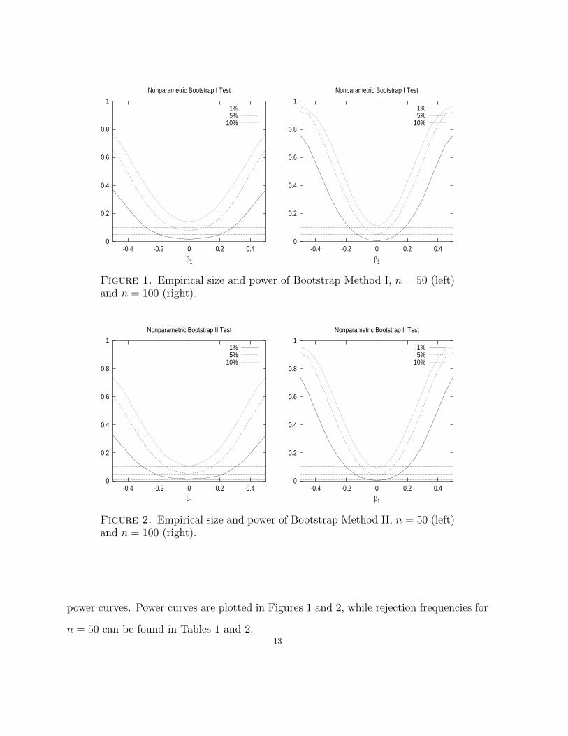
4.1. Size and Power of the Proposed Tests. In this section we report on a Monte

Carlo experiment designed to examine the finite-sample size and power of the proposed

test. The data generating process (DGP) we consider is a nonlinear function having

interaction between a discrete and continuous variable and is given by

(15) yi = β0 + β1zi1(1 + x2i ) + β2zi2 + β3xi + εi, i = 1, 2, . . . , n,

where z1 and z2 are both discrete binomial 0/1 random variables having Pr[zj = 1] = 0.5,

j = 1, 2, x ∼ N(0, 1), ε ∼ N(0, 1), and (β0, β1, β2, β3) = (1, β1, 1, 1).

We consider testing the significance of z1. Under the null (β1 = 0) that z1 is an irrelevant

regressor, the DGP is yi = β0 + β2zi2 + β3xi + εi. We assess the finite-sample size and

power of the test by varying β1, so that when β1 = 0 we can examine the test’s size while

when β1 6= 0 we can assess the test’s power.

We consider the performance of the proposed test using both bootstrap methods out-

lined above. We vary β1 in increments of 0.05 (0.0, 0.05, 0.10, . . . ) and compute the empir-

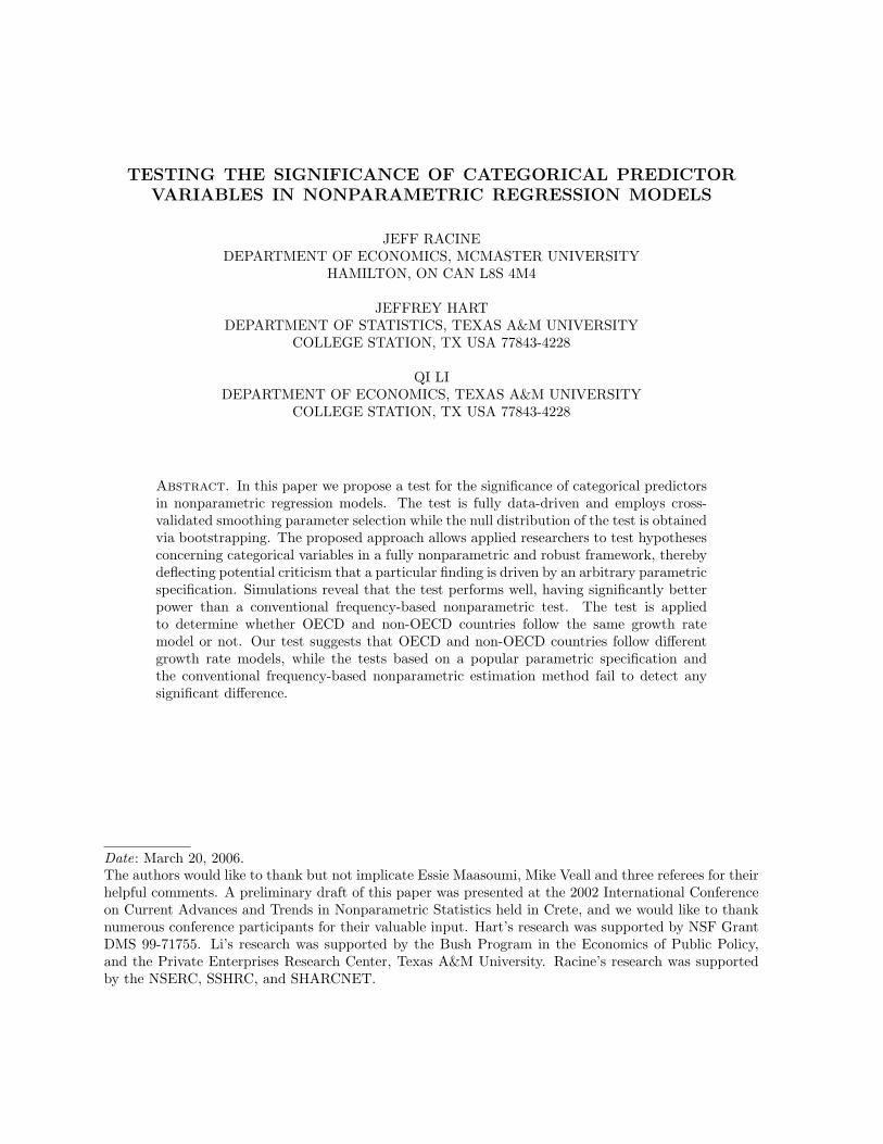
ical rejection frequency at nominal levels α = (0.01, 0.05, 0.10). We then construct smooth12

0

0.2

0.4

0.6

0.8

1

-0.4 -0.2 0 0.2 0.4β1

Nonparametric Bootstrap I Test

1% 5%

10%

0

0.2

0.4

0.6

0.8

1

-0.4 -0.2 0 0.2 0.4β1

Nonparametric Bootstrap I Test

1% 5%

10%

Figure 1. Empirical size and power of Bootstrap Method I, n = 50 (left)and n = 100 (right).

0

0.2

0.4

0.6

0.8

1

-0.4 -0.2 0 0.2 0.4β1

Nonparametric Bootstrap II Test

1% 5%

10%

0

0.2

0.4

0.6

0.8

1

-0.4 -0.2 0 0.2 0.4β1

Nonparametric Bootstrap II Test

1% 5%

10%

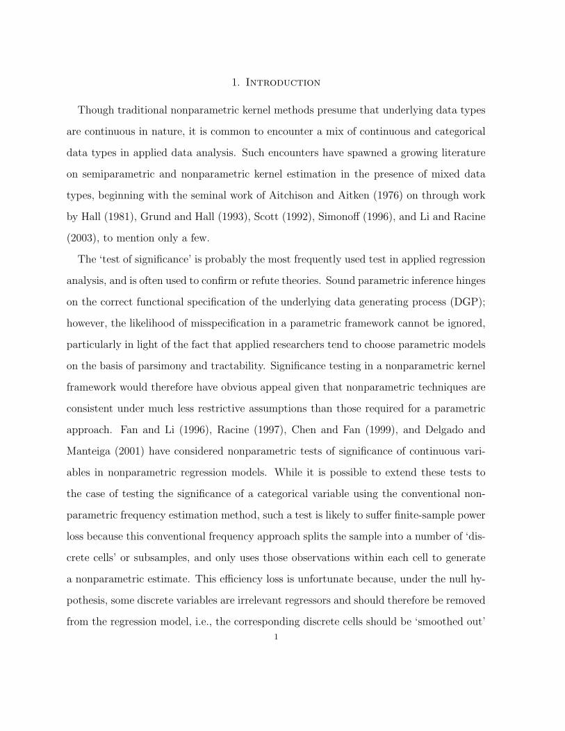
Figure 2. Empirical size and power of Bootstrap Method II, n = 50 (left)and n = 100 (right).

power curves. Power curves are plotted in Figures 1 and 2, while rejection frequencies for

n = 50 can be found in Tables 1 and 2.13

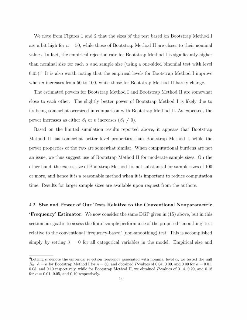
We note from Figures 1 and 2 that the sizes of the test based on Bootstrap Method I

are a bit high for n = 50, while those of Bootstrap Method II are closer to their nominal

values. In fact, the empirical rejection rate for Bootstrap Method I is significantly higher

than nominal size for each α and sample size (using a one-sided binomial test with level

0.05).3 It is also worth noting that the empirical levels for Bootstrap Method I improve

when n increases from 50 to 100, while those for Bootstrap Method II barely change.

The estimated powers for Bootstrap Method I and Bootstrap Method II are somewhat

close to each other. The slightly better power of Bootstrap Method I is likely due to

its being somewhat oversized in comparison with Bootstrap Method II. As expected, the

power increases as either β1 or n increases (β1 6= 0).

Based on the limited simulation results reported above, it appears that Bootstrap

Method II has somewhat better level properties than Bootstrap Method I, while the

power properties of the two are somewhat similar. When computational burdens are not

an issue, we thus suggest use of Bootstrap Method II for moderate sample sizes. On the

other hand, the excess size of Bootstrap Method I is not substantial for sample sizes of 100

or more, and hence it is a reasonable method when it is important to reduce computation

time. Results for larger sample sizes are available upon request from the authors.

4.2. Size and Power of Our Tests Relative to the Conventional Nonparametric

‘Frequency’ Estimator. We now consider the same DGP given in (15) above, but in this

section our goal is to assess the finite-sample performance of the proposed ‘smoothing’ test

relative to the conventional ‘frequency-based’ (non-smoothing) test. This is accomplished

simply by setting λ = 0 for all categorical variables in the model. Empirical size and

3Letting α denote the empirical rejection frequency associated with nominal level α, we tested the nullH0: α = α for Bootstrap Method I for n = 50, and obtained P -values of 0.04, 0.00, and 0.00 for α = 0.01,0.05, and 0.10 respectively, while for Bootstrap Method II, we obtained P -values of 0.14, 0.29, and 0.18for α = 0.01, 0.05, and 0.10 respectively.

14

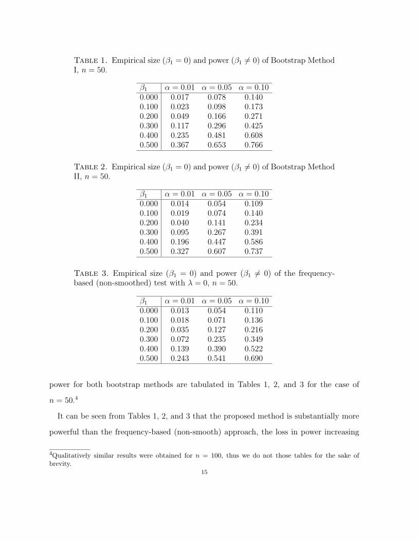
Table 1. Empirical size (β1 = 0) and power (β1 6= 0) of Bootstrap MethodI, n = 50.

β1 α = 0.01 α = 0.05 α = 0.100.000 0.017 0.078 0.1400.100 0.023 0.098 0.1730.200 0.049 0.166 0.2710.300 0.117 0.296 0.4250.400 0.235 0.481 0.6080.500 0.367 0.653 0.766

Table 2. Empirical size (β1 = 0) and power (β1 6= 0) of Bootstrap MethodII, n = 50.

β1 α = 0.01 α = 0.05 α = 0.100.000 0.014 0.054 0.1090.100 0.019 0.074 0.1400.200 0.040 0.141 0.2340.300 0.095 0.267 0.3910.400 0.196 0.447 0.5860.500 0.327 0.607 0.737

Table 3. Empirical size (β1 = 0) and power (β1 6= 0) of the frequency-based (non-smoothed) test with λ = 0, n = 50.

β1 α = 0.01 α = 0.05 α = 0.100.000 0.013 0.054 0.1100.100 0.018 0.071 0.1360.200 0.035 0.127 0.2160.300 0.072 0.235 0.3490.400 0.139 0.390 0.5220.500 0.243 0.541 0.690

power for both bootstrap methods are tabulated in Tables 1, 2, and 3 for the case of

n = 50.4

It can be seen from Tables 1, 2, and 3 that the proposed method is substantially more

powerful than the frequency-based (non-smooth) approach, the loss in power increasing

4Qualitatively similar results were obtained for n = 100, thus we do not those tables for the sake ofbrevity.

15

as β1 increases for the range considered herein. It would appear therefore that opti-

mal smoothing leads to finite-sample power gains for the proposed test relative to the

frequency-based (non-smoothed) version of the test.

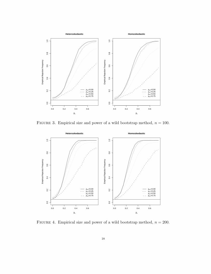
4.3. Size and Power Under Heteroskedastic Design and Correlated Regressors.

Next, we consider a modest Monte Carlo experiment designed to assess the performance

of the proposed test in two situations that one would expect to encounter in applied

settings:

• The relevant and irrelevant regressors are correlated, perhaps highly so.

• The disturbance vector is heteroskedastic,.

For this simulation, we consider another possible bootstrap scheme. Define the non-

parametric residuals

ei = yi − m(xi) − δ, i = 1, . . . , n,

where m(xi) = m(xi, zm), zm is the median of {zi}ni=1, and δ = n−1

∑ni=1(yi − m(xi)).

Let e∗1, . . . , e∗n be wild bootstrap errors generated by e∗i = [(1 −

√5)/2]ei with probability

r = (1 +√

5)/(2√

5), and e∗i = [(1 +√

5)/2]ei with probability 1 − r. If one wishes

to condition on the covariates, then a bootstrap sample would be (e∗i + m(xi), xi, zi),

i = 1, . . . , n, i.e, y∗i = m(xi) + e∗i , x∗

i = xi and z∗i = zi. If one wants to approximate the

unconditional distribution of the statistic, then the sample could be (e∗i + m(x∗i ), x

∗i , z

∗i ),

i = 1, . . . , n, where (x∗i , z

∗i ), i = 1, . . . , n, is a random sample from (xi, zi), i = 1, . . . , n.

The advantage of using a wild bootstrap, rather than the naıve resampling bootstrap, is

that the test will be robust to the presence of conditional heteroscedasticity.

We consider a simple linear DGP of the form

yi = α + βzzi + βxxi + εi, i = 1, 2, . . . , n,16

where zi ∈ {−1, 0, 1} with Pr(zi = l) = 1/3, l = 1, 2, 3, and where xi ∼ U [−2, 2] with

ρxz = 0.00, 0.25, 0.50, 0.75 being the correlation between xi and zi. We consider two error

processes, one with εi ∼ N(0, 1) and one with εi ∼ N(0, σ2i ) with σi = 1 + sin(xi)/4.

We arbitrarily set (α, βz, βx) = (1, βz, 1) and vary βz between 0 and 3/4 to examine

finite-sample size and power. We also consider a range of sample sizes.

In particular, we varied βz so that it assumed values (0.00, 0.05, . . . , 0.75). For each

Monte Carlo replication, bandwidths were selected via cross-validation, then 399 wild

bootstrap replications were conducted to obtain the null distribution for each test, at

which point the empirical P value was computed, which we denote P . The null was

rejected for nominal size α if P < α. There were 1,000 Monte Carlo replications conducted

for each value of βz. A range of sample sizes were considered, and results are presented

in the form of empirical half-power curves. By way of example, we present results for

α = 0.05. Qualitatively similar results were obtained for all conventional values of α.

Note that the results that follow use the same cross-validated bandwidths for each wild

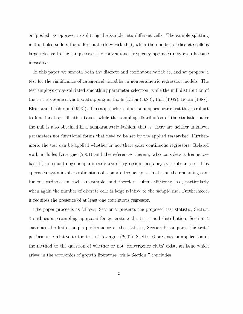
bootstrap replication (i.e., it is a Bootstrap I type test). Results are summarized in figures

3 and 4 .

As can be seen, the test appears to be robust to the presence of heteroskedasticity,

while correlation between the variable being tested and the remaining variables reduces

power as expected but do not affect empirical size. The test is slightly oversized for small

samples, but this disappears quite quickly.

4.4. The Standardized Test. In addition to the experiments reported above, we also

implemented a standardized version of our test, the tn test, as described at the end of

Section 3. Compared with the non-standardized test In using Bootstrap Method I, the use

of tn in this case yields small improvements in nominal size as expected and also appears17

0.0 0.2 0.4 0.6

0.0

0.2

0.4

0.6

0.8

1.0

Heteroskedastic

βz

Em

piric

al R

ejec

tion

Freq

uenc

y

ρxz=0.00ρxz=0.25ρxz=0.50ρxz=0.75

0.0 0.2 0.4 0.60.

00.

20.

40.

60.

81.

0

Homoskedastic

βz

Em

piric

al R

ejec

tion

Freq

uenc

y

ρxz=0.00ρxz=0.25ρxz=0.50ρxz=0.75

Figure 3. Empirical size and power of a wild bootstrap method, n = 100.

0.0 0.2 0.4 0.6

0.0

0.2

0.4

0.6

0.8

1.0

Heteroskedastic

βz

Em

piric

al R

ejec

tion

Freq

uenc

y

ρxz=0.00ρxz=0.25ρxz=0.50ρxz=0.75

0.0 0.2 0.4 0.6

0.0

0.2

0.4

0.6

0.8

1.0

Homoskedastic

βz

Em

piric

al R

ejec

tion

Freq

uenc

y

ρxz=0.00ρxz=0.25ρxz=0.50ρxz=0.75

Figure 4. Empirical size and power of a wild bootstrap method, n = 200.

18

to lead to a small reduction in power.5 Recall that the In test based on Bootstrap Method

I is slightly oversized. Thus, this power reduction may reflect the difference in estimated

sizes. Indeed simulations (not reported here) show that the size-adjusted powers of the

In and the tn tests are virtually identical. The use of tn based on a nested bootstrap

procedure increases the computational burden of the proposed approach by an order of

magnitude; hence, we conclude that standardizing the test does not appear to be necessary

to achieve reasonable size and power in this setting.

5. Comparison with Existing Tests

The only existing kernel-based test statistic we are aware of that can be compared

with the proposed test without modification is that of Lavergne (2001), who proposes a

nonparametric test for equality of regression across subsamples. We compare the power

of our smooth Bootstrap II test with his frequency-based (non-smooth) test which is

essentially a nonparametric Chow test (see Lavergne (2001) for details). Lavergne (2001)

presents a wide array of simulation results, and so for the sake of brevity we restrict

our attention to the first set of results he reports and consider a subset of his range of

alternatives. We implement the Monte Carlo experiment reported in Lavergne (2001)

(page 326, Table 1). Data was generated through

(16) yi = βx + γx3 + I(C = 0)d(X) + ε,

where conditional on C, x is N(C, 1), and ε is independently distributed as N(0, 1), with

β = −4, γ = 1, and d(X) = ηX with η = 0, 0.5, 1, 2 corresponding respectively to DGP0,

DGP1, DGP2, and DGP3. DGP0 corresponds to the null hypothesis d(X) ≡ 0, and DGP1

through DGP3 allow us to compare power. We also consider the parametric Chow test

reported in Lavergne (2001) which serves as a benchmark upper bound on performance.

5These simulation results are not reported here to save space. The results are available from the authorsupon request.

19

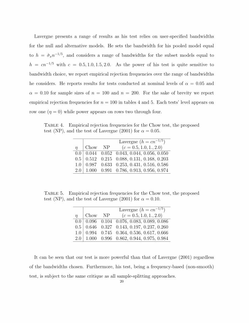
Lavergne presents a range of results as his test relies on user-specified bandwidths

for the null and alternative models. He sets the bandwidth for his pooled model equal

to h = σxn−1/5, and considers a range of bandwidths for the subset models equal to

h = cn−1/5 with c = 0.5, 1.0, 1.5, 2.0. As the power of his test is quite sensitive to

bandwidth choice, we report empirical rejection frequencies over the range of bandwidths

he considers. He reports results for tests conducted at nominal levels of α = 0.05 and

α = 0.10 for sample sizes of n = 100 and n = 200. For the sake of brevity we report

empirical rejection frequencies for n = 100 in tables 4 and 5. Each tests’ level appears on

row one (η = 0) while power appears on rows two through four.

Table 4. Empirical rejection frequencies for the Chow test, the proposedtest (NP), and the test of Lavergne (2001) for α = 0.05.

Lavergne (h = cn−1/5)η Chow NP (c = 0.5, 1.0, 1., 2.0)0.0 0.044 0.052 0.043, 0.044, 0.056, 0.0500.5 0.512 0.215 0.088, 0.131, 0.168, 0.2031.0 0.987 0.633 0.253, 0.431, 0.516, 0.5862.0 1.000 0.991 0.786, 0.913, 0.956, 0.974

Table 5. Empirical rejection frequencies for the Chow test, the proposedtest (NP), and the test of Lavergne (2001) for α = 0.10.

Lavergne (h = cn−1/5)η Chow NP (c = 0.5, 1.0, 1., 2.0)0.0 0.096 0.104 0.076, 0.083, 0.089, 0.0860.5 0.646 0.327 0.143, 0.197, 0.237, 0.2601.0 0.994 0.745 0.364, 0.536, 0.617, 0.6662.0 1.000 0.996 0.862, 0.944, 0.975, 0.984

It can be seen that our test is more powerful than that of Lavergne (2001) regardless

of the bandwidths chosen. Furthermore, his test, being a frequency-based (non-smooth)

test, is subject to the same critique as all sample-splitting approaches.20

6. Application - ‘Growth Convergence Clubs’

Quah (1997) and others have examined the issue of whether there exist ‘convergence

clubs,’ that is, whether growth rates differ for members of clubs such as the Organization

for Economic Cooperation and Development (OECD) among others. We do not attempt

to review this vast literature here; rather, we refer the interested reader to Mankiw et

al. (1992), Liu and Stengos (1999), Durlauf and Quah (1999) and the references therein.

We apply the proposed test to determine whether OECD countries and non-OECD

countries follow the same growth model. This is done by testing whether OECD member-

ship (a binary categorical variable) is a relevant regressor in a nonparametric framework.

The null hypothesis is that the OECD membership is an irrelevant regressor; thus, under

the null, OECD and non-OECD countries’ growth rates are all determined by the same

growth model. The alternative hypothesis is the negation of the null hypothesis. That is,

OECD and non-OECD countries have different growth rate (regression) models.

When using parametric methods, if the regression functional form is misspecified one

may obtain misleading conclusions. By using methods that are robust to functional

specification issues we hope to avoid criticism that findings are driven by a particular

functional form presumed.

Following Liu and Stengos (1999), we employ panel data for 88 countries over seven

(five-year average) periods (1960-1964, 1965-1969, 1970-1974, 1975-1979, 1980-1984, 1985-

1989 and 1990-1994) yielding a total of 88 × 7 = 616 observations in the panel. We then

construct our test based on the following model:

(17)

growthit = m(OECDit, DTt, ln(invit), ln(popgroit), ln(initgdpit), ln(humancapit))+εit,

21

where growthit refers to the growth rate of income per capita during each period, DTt the

seven period dummies, invit the ratio of investment to Gross Domestic Product (GDP),

popgroit growth of the labor force, initgdpit per capita income at the beginning of each

period, and humancapit human capital. Initial income estimates are from the Summers-

Heston (1988) data base, as are the estimates of the average investment/GDP ratio for

five-year periods. The average growth rate of per capita GDP and the average annual

population growth rate for each period are from the World Bank. Finally, human capital

(average years of schooling in the population above 15 years of age) is obtained from Barro

and Lee (2000).

Before we report results for our smoothing-based nonparametric test, we first consider

some popular parametric methods for approaching this problem. A common parametric

approach is to employ a linear regression model, with the OECD dummy variable being

one possible regressor, and then to test whether the coefficient on this dummy variable is

significant. We consider a parametric specification suggested by Liu and Stengos (1999),

which contains dummy variables for OECD status and is nonlinear in the initial GDP

and human capital variables.6

(18)

growthit = β0OECDit +7

∑

s=1

βsDTs + β8 ln(invit) + β9 ln(popgroit)

+4

∑

s=1

αs[ln(initgdpit)]s +

3∑

s=1

γs[ln(humancap)it)]s + εit.

Estimation results for model (18) are given in Table 6, while the t-statistic for the

OECD dummy is -0.973 having a P -value of 0.33.7 Thus, the parametric test fails to

reject the null.

6We are grateful to Thanasis Stengos for providing data and for suggesting this parametric specificationbased upon his work in this area.7R code and data needed for the replication of these parametric results are available from the authorsupon request.

22

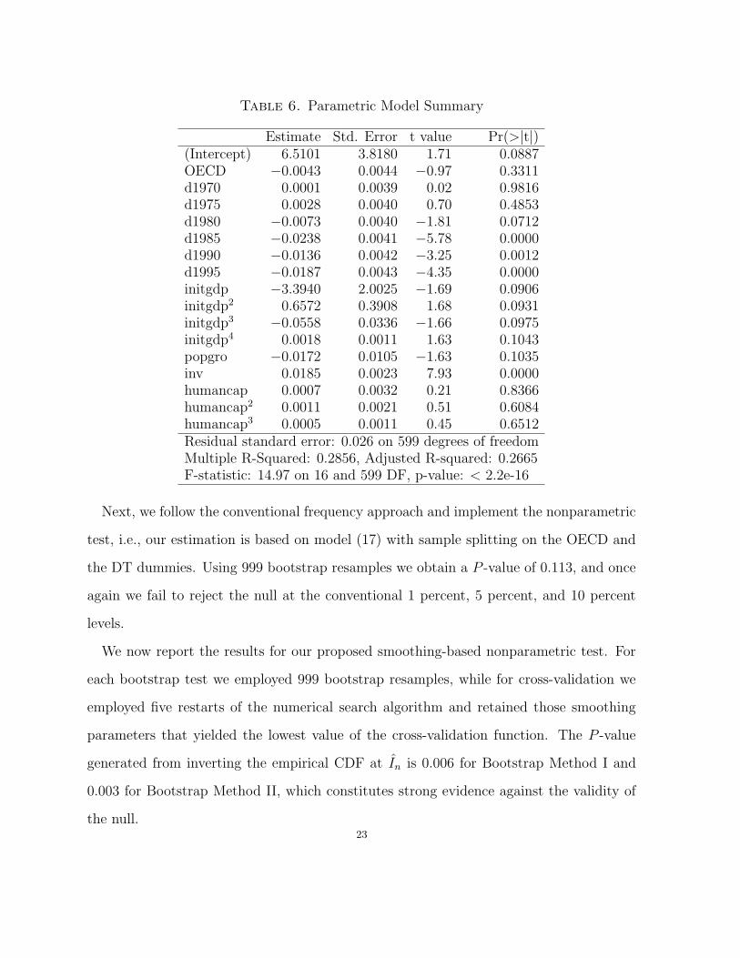
Table 6. Parametric Model Summary

Estimate Std. Error t value Pr(>|t|)(Intercept) 6.5101 3.8180 1.71 0.0887OECD −0.0043 0.0044 −0.97 0.3311d1970 0.0001 0.0039 0.02 0.9816d1975 0.0028 0.0040 0.70 0.4853d1980 −0.0073 0.0040 −1.81 0.0712d1985 −0.0238 0.0041 −5.78 0.0000d1990 −0.0136 0.0042 −3.25 0.0012d1995 −0.0187 0.0043 −4.35 0.0000initgdp −3.3940 2.0025 −1.69 0.0906initgdp2 0.6572 0.3908 1.68 0.0931initgdp3 −0.0558 0.0336 −1.66 0.0975initgdp4 0.0018 0.0011 1.63 0.1043popgro −0.0172 0.0105 −1.63 0.1035inv 0.0185 0.0023 7.93 0.0000humancap 0.0007 0.0032 0.21 0.8366humancap2 0.0011 0.0021 0.51 0.6084humancap3 0.0005 0.0011 0.45 0.6512Residual standard error: 0.026 on 599 degrees of freedomMultiple R-Squared: 0.2856, Adjusted R-squared: 0.2665F-statistic: 14.97 on 16 and 599 DF, p-value: < 2.2e-16

Next, we follow the conventional frequency approach and implement the nonparametric

test, i.e., our estimation is based on model (17) with sample splitting on the OECD and

the DT dummies. Using 999 bootstrap resamples we obtain a P -value of 0.113, and once

again we fail to reject the null at the conventional 1 percent, 5 percent, and 10 percent

levels.

We now report the results for our proposed smoothing-based nonparametric test. For

each bootstrap test we employed 999 bootstrap resamples, while for cross-validation we

employed five restarts of the numerical search algorithm and retained those smoothing

parameters that yielded the lowest value of the cross-validation function. The P -value

generated from inverting the empirical CDF at In is 0.006 for Bootstrap Method I and

0.003 for Bootstrap Method II, which constitutes strong evidence against the validity of

the null.23

The inconsistency of the parametric test and our proposed nonparametric test also

suggests that the parametric model is misspecified. Applying the parametric regression

specification error test for correct specification of Ramsey (1969) yields a test statistic

having a P -value of 0.0225 suggesting that functional form of the model is incorrect. We

also applied a consistent nonparametric test for correct specification of the parametric

model (see Hsiao, Li, and Racine (2003)). The P -value from this test was 0.0008 and we

again reject the null of correct parametric specification.

The reason why the conventional frequency based nonparametric test also fails to reject

the null is that it splits the sample into 2 × 7 = 14 parts (the number of discrete cells

from the discrete variables OECD and DT) when estimating the nonparametric regression

functions; thus, the much smaller (sub) sample sizes lead to substantial finite sample power

loss for a test based on the conventional frequency approach.

We conclude that there is robust nonparametric evidence in favor of the existence of

‘convergence clubs,’ a feature that may remain undetected when using both common

parametric specifications and conventional nonparametric approaches. That is, growth

rates for OECD countries appear to be different from those for non-OECD countries.

7. Conclusion

In this paper we propose a test for the significance of categorical variables for non-

parametric regression. The test is fully data-driven and uses resampling procedures for

obtaining the null distribution of the test statistic. Three resampling methods (Bootstrap

Methods I, II and the heteroskedastic robust bootstrap method) for generating the test

statistic’s null distribution are proposed, and all appear to perform well in finite-sample

settings. Monte Carlo simulations suggest that the test is well-behaved in finite samples,

having correct size and power that increases with the degree of departure from the null

and with the sample size. The test is more powerful (in finite-sample applications) than24

a conventional frequency-based (non-smoothing) version of the test, indicating that op-

timal smoothing of categorical variables is desirable not only for estimation but also for

inference. An application demonstrates how one can test economic hypotheses concern-

ing categorical variables in a fully nonparametric and robust framework, thereby parrying

the thrusts of critics who might argue that the outcome was driven by the choice of a

parametric specification.

References

Ahmad, I. A. and P. B. Cerrito (1994), “Nonparametric estimation of joint discrete-

continuous probability densities with applications,” Journal of Statistical Planning and

Inference, 41, 349-364.

Aitchison, J. and C. G. G. Aitken (1976), “Multivariate binary discrimination by the

kernel method,” Biometrika, 63, 413-420.

Barro, R. and J. W. Lee (2000), “International Data on Educational Attainment: Updates

and Implications,” Working paper No. 42, Center for International Development, Harvard

University.

Beran, R. (1988), “Prepivoting test statistics: A bootstrap view of asymptotic refine-

ments,” Journal of the American Statistical Association, 83, 687-697.

Chen, X. and Y. Fan (1999), “Consistent Hypothesis Tests in Nonparametric and Semi-

parametric Models for Econometric Time Series,” Journal of Econometrics, 91, 373-401.

Delgado, M.A. and W.G. Manteiga (2001), “Significance testing in nonparametric regres-

sion based on the bootstrap,” Annals of Statistics, 29, 1469-507.

Durlauf, S. N., and D. T. Quah (1999), “The New Empirics of Economic Growth,” Chapter

4, of J. B. Taylor and M. Woodford (eds.), Handbook of Macroeconomics I, Elsevier

Sciences, 235-308.

Efron, B. (1983), The Jackknife, the Bootstrap, and Other Resampling Plans, Philadel-

phia, Society for Industrial and Applied Mathematics.

Efron, B. and R. J. Tibshirani (1993), An Introduction to the Bootstrap, New York,

London, Chapman and Hall.25

Fan, Y. and Q. Li (1996), “Consistent model specification tests: omitted variables and

semiparametric functional forms,” Econometrica, 64, 865-890.

Hall, P. (1992), The Bootstrap and Edgeworth Expansion, New York, Springer Series in

Statistics, Springer-Verlag.

Hall, P. and K. H. Kang (2001), “Bootstrapping nonparametric density estimators with

empirically chosen bandwidths,” Annals of Statistics, 29, 1443-1468.

Hall, P. and J. Racine and Q. Li (forthcoming), “Cross-validation and the estimation of

conditional probability densities,” Journal of American Statistical Association.

Hall, P. and Q. Li and J. Racine (2004), “Nonparametric Estimation of Regression Func-

tions in the Presence of Irrelevant Regressors,” Manuscript.

Hart, J. and T. E. Wehrly (1992), “Kernel regression when the boundary region is large,

with an application to testing the adequacy of polynomial models,” Journal of American

Statistical Association, 87, 1018-1024.

Hsiao, C., Q. Li and J. S. Racine (2003), “A Consistent Model Specification Test with

Mixed Categorical and Continuous Data,” revised and resubmitted to the International

Economic Review.

Lavergne, P. (2001), “An Equality Test Across Nonparametric Regressions,” Journal of

Econometrics, 103, 307-344.

Li, Q. and J. S. Racine (2003), “Nonparametric estimation of distributions with categorical

and continuous data,” Journal of Multivariate Analysis, 86, 266-292.

Li, Q. and S. Wang (1998), “A Simple Bootstrap Test for a Parametric Regression Func-

tion,” Journal of Econometrics, 87, 145-165.

Liu, Z. and T. Stengos (1999), “Non-linearities in cross country growth regressions: a

semiparametric approach,” Journal of Applied Econometrics, 14, 527-538.

Mankiw, N., Romer, D. and D. Weil (1992), “A contribution to the empirics of economic

growth,” Quarterly Journal of Economics, 108, 407-437.

Quah, D. T. (1997), “Empirics for growth and distribution: stratification, polarization

and convergence clubs,” Journal of Economic Growth, 2, 27-59.

Ramsey J. B. (1969), “Tests for Specification Error in Classical Linear Least Squares

Regression Analysis,” Journal of the Royal Statistical Society, Series B 31, 350-371.26

Racine, J. S. (1997), “Consistent significance testing for nonparametric regression,” Jour-

nal of Business and Economic Statistics, 15 (3), 369-379.

Racine, J. S. (2002), “Parallel distributed kernel estimation,” Computational Statistics

and Data Analysis, 40 (2), 293–302.

Racine, J. S. and Q. Li (2004), “Nonparametric estimation of regression functions with

both categorical and continuous data,” Journal of Econometrics, 119 (1), 99-130.

Robinson, P. M. (1991), “Consistent nonparametric entropy-based testing,” Review of

Economic Studies, 58, 437-453.

Summers, R. and A. Heston (1988), “A new set of international comparisons of real

product and prices: Estimates for 130 countries,” Review of Income and Wealth, 34, 1-26.

27