S0ren Johansen

Anders Rygh Swensen

TESTING RATIONAL

EXPECTATIONS IN VECTOR

AUTOREGRESSIVE MODELS

Institute of Mathematical Statistics University of Copenhagen

Testing'rational expectations in vector autoregressive models" *

Soren J ohansen University of Copenhagen Anders Rygh Swensen Statistics Norway and University of Oslo

Abstract

Assuming that the solutions of a set of restrictions on the rational ex­pectations of future values can be represented as a vector autoregressive model, we study the implied restrictions on the coefficients. Nonstationary behavior of the variables is allowed, and the restrictions on· the cointegra­tion relationships are spelled out. In some interesting special cases it is shown that the likelihood ratio statistic can easily be computed.

1 Introduction

Expectations play a central role in many economic theories. But the incorpo­ration of this kind of variables in empirical models rises many problems. The variables are in many cases unobserved either because data on expectations are unavailable, or because there may often be reason to suspect that the available data on expectations are unreliable. There are also problems connected with the validity. Economic agents may benefit from not revealing their real expectations. Some sort of proxies must therefore be used.

One possibility when the models contain stochastic elements, is to use con­ditional expectations in the probabilistic sense given some previous information. When this information is all available past and present information contained in the variables of the model, rational expectation is the usual d~·nominatlon. Another, perhaps more precise, name is model consistent expectations. Then the aspect that the expectations mean conditional expectations in the model the analysis is based upon, is emphasized. This is an idea originally introduced by Muth [12J and [13J. However, since rational expectation seems to be the common name of this type of expectations, we shall stick to this usage in the following.

*We want to thank Niels Haldrup for drawing our attention to restrictions involving lagged variables and M. Hashem Pesaran for suggesting a simplification of the treatment of present value models.

1

It is well known that dynamic models containing rational expectations of fu­ture values have a multitude of solutions. In a recent paper Baillie [2J advocated a procedure for testing restrictions between future rational expectations of a set of variables by assuming that the solutions could be described by a vector au­toregressive (VAR) model. He then expressed the restrictions implied by the postulated relationships between the expectations as restrictions on the coeffi­cients of the VAR model.

In this paper we shall follow the same approach. However, Baillie also allowed for non-stationary behaviour of the variables that could be eliminated by first transforming the variables using known cointegrating relationships. Thus some knowledge about how the variables cointegrate is necessary. At this point we shall pursue another line. Starting out with the V AR model we only assume that the variables are integrated of order one. It turns out, as one can expect, that the restrictions on the expectations entail restrictions on the cointegration relationships. In addition some restrictions on the short run part of the model must be satisfied.

These implications can be tested by invoking the results of Johansen [8] and [9] and of Johansen and Juselius [10] and [11]. In general it seems that a two step procedure must be used, but in an interesting special case it is possible to find the likelihood ratio test. What is also of interest, is that this test is easy to compute involving by now well known reduced rank regression procedures.

The paper is organized as follows: In the next section we state the type of relationships between the expectations we shall consider, and derive the impli­cations for the VAR model when the expectations are considered to be rational in the sense described earlier. In section 3 we treat the special case where a likelihood ratio test can be developed. Finally, assuming that the variables are integrated of order 1 we discuss the asymptotic distribution of the tests.

2 The form of the restrictions.

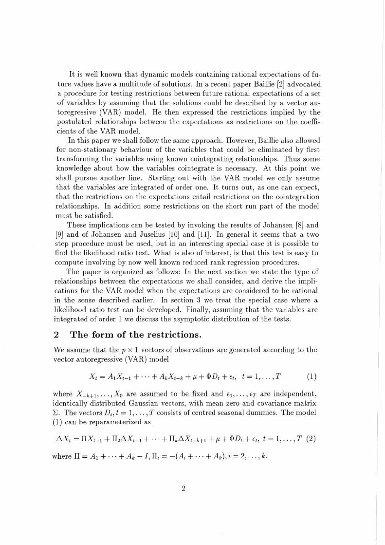
We assume that the p x 1 vectors of observations are generated according to the vector autoregressive (VAR) model

where X-HI, ... ,Xo are assumed to be fixed and El, ... , ET are independent, identically distributed Gaussian vectors, with mean zero and covariance matrix ~. The vectors D t , t = 1, ... ,T consists of centred seasonal dummies. The model (1) can be reparameterized as

where IT = Al + ... + Ak - I, ITi = -(Ai + ... + Ak), i = 2, ... ,k.

2

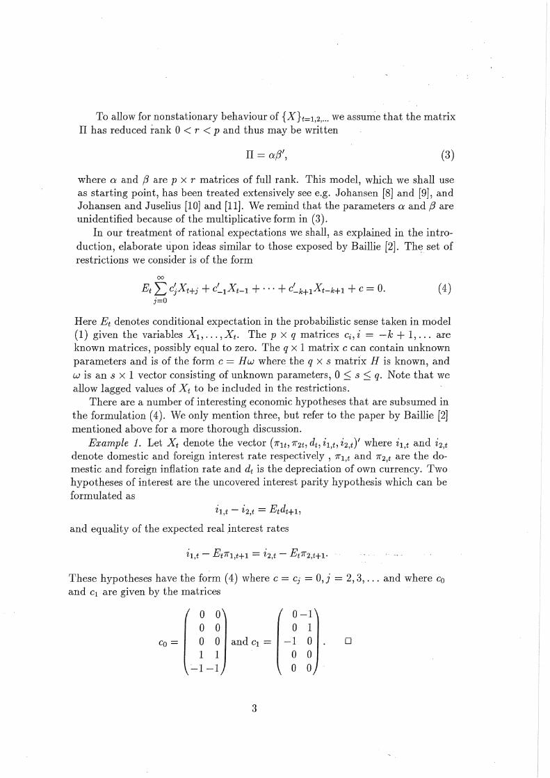
To allow for nonstationary behaviour of {X}t=I,2, ... we assume that the matrix IT has reduced rank 0 < r < p and thus may be written

IT = ex(3', (3)

where ex and (3 are p X r matrices of full rank. This model, which we shall use as starting point, has been treated extensively see e.g. Johansen [8] and [9], and Johansen and Juselius [10] and [11]. We remind that the parameters ex and (3 are unidentified because of the multiplicative form in (3).

In our treatment of rational expectations we shall, as explained in the intro­duction, elaborate upon ideas similar to those exposed by Baillie [2]. The set of restrictions we consider is of the form

00

Et 2: cjXt+j + c~IXt-1 + ... + C~k+IXt-k+1 + c = O. j=O

(4)

Here Et denotes conditional expectation in the probabilistic sense taken in model (1) given the variables Xl, .. . , Xt. The p x q matrices Ci, i = -k + 1, ... are known matrices, possibly equal to zero. The q X 1 matrix C can contain unknown parameters and is of the form C = Hw where the q X s matrix H is known, and w is an s X 1 vector consisting of unknown parameters, 0 :S s :S q. Note that we allow lagged values of X t to be included in the restrictions.

There are a number of interesting economic hypotheses that are subsumed in the formulation (4). We only mention three, but refer to the paper by Baillie [2] mentioned above for a more thorough discussion.

Example 1. Let X t denote the vector (1flt' 1f2t, dt , il,t, i2,t)' where il,t and i2,t denote domestic and foreign interest rate respectively, 1f1,t and 1f2,t are the do­mestic and foreign inflation rate and dt is the depreciation of own currency. Two hypotheses of interest are the uncovered interest parity hypothesis which can be formulated as

and equality of the expected real interest rates

These hypotheses have the form (4) where C = Cj = O,j = 2,3, ... and where Co

and Cl are given by the matrices

0 0 0-1 0 0 0 1

Co = 0 0 and Cl = -1 0 0

1 1 0 0 ~1-1 0 0

3

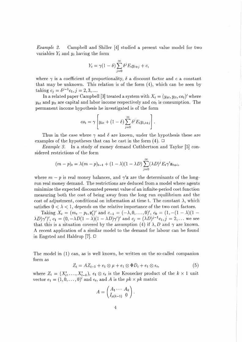
Example 2. Campbell and Shiller [4J studied a present value model for two variables Yt and Yt having the form

00

Yt = ,(I - 5) L 5j EtYHj + C,

j=O

where, is a coefficient of proportionality, 5 a discount factor and c a constant that may be unknown. This relation is of the form (4), which can be seen by taking Cj = 5j - l c!,] = 2,3, ....

In a related paper Campbell [3] treated a system with X t = (Ykt, Ylt, cot}' where Ykt and YZt are capital and labor income respectively and COt is consumption. The permanent income hypothesis he investigated is of the form

COt = "I [Ykt + (1 - 5) f 5j EtYZ,Hj]. J=O

Thus in the case where, and 5 are known, under the hypothesis these are examples of the hypotheses that can be cast in the form (4). 0

Example 3. In a study of money demand Cuthbertson and Taylor [5J con­sidered restrictions of the form

00

(m - p)t = A(m - P)t-l + (1 - A)(l - AD) L(AD)j Et1'ZHi, j=O

where m - P is real money balances, and ,'z are the determinants of the long­run real money demand. The restrictions are deduced from a model where agents minimize the expected discounted present value of an infinite-period cost function measuring both the cost of being away from the long run equilibrium and the cost of adjustment, conditional on information at time t. The constant A, which satisfies 0 < A < 1, depends on the relative importance of the two cost factors.

Taking X t = (mt - Pt, zD' and Cl = (-A, 0, ... ,0)', Co = (1, -(1 - A)(l -AD)"!')', Cl = (0, -AD(l - A)(l - AD)"!')' and Cj = (AD)j-lCI,] = 2, ... we see that this is a situation covered by the assumption (4) if A, D and, are known. A recent application of a similar model to the demand for labour can be found in Engsted and Haldrup [7J. 0

The model in (1) can, as is well known, be written on the so-called companion form as

(5)

where Zt = (X;, ... , X;_k)' el 0 Et is the Kronecker product of the k x 1 unit vector el = (1,0, ... ,0)' and Et, and A is the pk X pk matrix

( Al ... Ak) A = Ip(k-l) 0 .

4

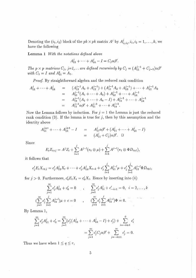
Denoting the (il' i2) block of the pk X pk matrix Aj by A{ i ,iI, i2 = 1, ... , k, we , 1, 2

have the following

Lemma 1 With the notations defined above

A{l + ... + A~k - I = Cj o:f3'.

The p X P matrices Cjl j=l}" .. are defined recursively by Cj = (A~ll + Cj - l )o:f3' with Cl = I and Atl = Al'

Proof. By straightforward algebra and the reduced rank condition

A~l + ... + A~k (A~ll Al + A~~l) + (A~ll A2 + A~31) + ... + A~ll Ak

A{11(A1 + ... + Ak) + A{~l + ... + Ai:;;l

A{ll(Al + ... + Ak - 1) + A{ll + ... + A~kl A{llo:f3' + A{ll + ... + A{kl .

Now the Lemma follows by induction. For j = 1 the Lemma is just the reduced rank condition (3). If the lemma is true for j, then by this assumption and the identity above

Since

A{tl + ... + A~tl - I A{lo:fJ' + (A{l + ... + Aik - I)

(A{t + Cj )o:f3'. 0

j j

EtZHj = Aj Zt + I: Aj-I (el ® f-l) + I: Aj-I (el ® <I> DH1 ), 1=1 1=1

it follows that j j

'E X 'Aj X + +' Aj X +' '\"""' Aj-I + ,'\"""' Aj-I ffiD Cj t Hj = Cj 11 t . . . cj lk t-k Cj L.t 11 f-l cj L.t 11 'J" Ht, 1=1 1=1

for j > O. Furthermore, c~EtXt = C~Xt. Hence by inserting into (4)

00 00

LcjA{l + c~ = 0 L cjA{i + C~i+t = 0, i = 2, ... ,k j=1 j=l

00 j 00 j

(I: cj I: A{ll)fL + c = 0 (I: cj I: A{ll).p = O. j=l 1=1 j=l 1=1

By Lemma 1,

00 00 0

I: cjA~l + C~ = I:(Cj(A{l + ... + A{k - 1) + cj) + L c~ j=l j=l i=-k+l

00 00

= L cjCjo:fJ' + L cj = O. j=l j=-k+l

Thus we have when 1 ::; q ::; r,

5

Proposition 1 . The restrictions on the coefficients in the reduced rank VAR model implied by the hypothesis {4} are equivalent to

(i) (6)

( ~~) ",00 'Aj - , '-2 k bb uj=l Cj 1i - -c-i+1' Z - , ... , ,

",00 I ",j Aj-l - H ",00 I ",j Aj-l ifi. - ° uj=l Cj ul=l 11 f1 - - w, uj=l Cj ul=l 11 '¥ - ,

where Cj and At, i = 1, ... ,k, j = 1,2, ... are as defined in Lemma 1 and A~l = I.

The infinite sums appearing in the expressions above are all assumed to exist. In case they do not converge, the restriction (6) does not make sense. In many special situations convergence is no problem. The eigenvalues of A then have all modulus less than or equal to 1, and the sum L~-k+1 Cj either consists of a finite sum of non-zero terms or of exponentially decreasing terms.

One can also remark that the conditions of the first part of the proposition may be formulated as L~-k+1 Cj E sp((3), i.e. the vector L~-k+1 Cj must belong to the space spanned by the columns of (3. Also by multiplying both sides with the matrix ((3'(3)-1 (3', one has the following restrictions on the adjustment parameters

. , "'00 C' - ((3'(3)-1(3' ",00 (Y. (Y uj=l jCj - - uj=-k+1 Cj.

The restrictions on the (Y parameters and the conditions in the second part of Proposition 1 are in general non-linear in terms of the parameters of the VAR model in (1) or (2). In the particular case where C2 = C3 = ... = 0, the conditions in Proposition 1 simplify since Cl = A~l = I and the terms involving the other Cjs disappear.

Corollary 1 If Ci = 0, i = 2, . "! the conditions of Proposition 1 take the form in terms of the model {2}:

(i) (3 ' - ",1 (Y Cl - - uj=-k+1 Cj (7)

(ii) c~IIi = Lj=i C~j+1' i = 2, ... , k,

C~f1 = -Hw and c~ <I> = 0.

That restrictions like those of example 1 are covered by Corollary 1 is evident. What may not be so obvious, is that the restrictions in the other two examples, where Cj = 8j - 1cl,j = 2, ... , are also covered. To see that, write the restrictions (4) as

00 k-1 C~Xt + EtC~Xt+1 + 8 L 8j- 2 Etc~Xt+j + L C~jXt_j + C = 0. (8)

j=2 j=l Using iterated conditional expectations in a similar expression at time t + 1,

multiplying by 8 and subtracting from (8) yields

(co - 8C1)'Xt + (Cl - bco)'EtX t+1 + k-2 2)c-j - 8c(j+1))'Xt- j + C~k+1Xt-k+l + (1 - 8)c = 0, j=l

6

which shows that also restrictions in examples 2 and 3 have a form covered by Corollary 1. .

In the next section we shall derive the likelihood ratio test for restrictions of this particular type. To discuss this problem the following result turns out to be useful. We introduce the notation that if a is a p X q matrix of full rank q, then a.L is a p X (p - q) matrix so that the square matrix (a, a.L) is non-singular. Also let a = a(a'a)-l. Then the result can be formulated as:

Proposition 2 The p x p matrix II has reduced rank r and satisfies

ll'b = d (9)

where band dare p X q matrices of full rank if and only if IT has the form

II = bd' + b.t1](d~ + b.L 8d' (10)

where ry and e are matrices of dimension (p - q) X (r - q) and of full rank (r - q).

Proof. Assuming that (9) is true we consider

, [b'lld b'lld.L 1 [d' dOl (b, b.L) II (d, d.L) = b~ lld b~ lld.L = b~ lld b~ lld.L .

If IT has rank r, then r 2:: q , which is the rank of d'd. Then b~IId.L must have rank r - q, and can be written b~ IId.L = rye for matrices of rank r - q. If we define the (p - q) X q matrix e as 8 = b~lld, we get the representation

II = (b, bd [ ~d ry~' 1 (d, d.L)' = bd' + b.L 8d' + b.L rye d/.

which proves one part of the proposition. Next assume that IT can be represented as in (10). Then bill = d'. That the

rank is reduced can be seen from

which has rank equal to rank(d'd) + rank(rye) = q + (r - q) = r.D

3 Derivation of the maximum likelihood estimators and the likelihood ratio test in a special case.

We consider a situation similar to the one covered by Corollary 1, i.e Cj = 0, j = 2,3, ... , and Co and Cl are known p x q matrices. For simplicity we also assume that C2 = ... = Ck = 0, so that the restrictions only involve one lagged variable. Also we make the additional assumption that b = Cl and d = -(Cl + Co + Cl)

are of full rank. Let a = b.L.

7

Using the results of Proposition 2 in model (2) with band d as just defined yields the equation

bd'Xt- 1 + arye'dJ..'Xt- 1 + a8a'Xt- 1 (11)

+ II26.Xt- 1 + ... + II k 6.Xt- k - 1 + f-l + 1> Dt + Et·

By multiplying (11) with a' and b' we get after taking the restrictions in Corollary 1 into account

+ +

rye d/ X t - 1 + 8a' X t - 1

a'II26.Xt- 1 + ... + a'IIk 6.Xt- k - 1

a' f-l + a'1>Dt + a' Et

d'Xt- 1 + C~l6.Xt-l - Hw + b'Et.

(12)

(13)

We thus end up with a model (12)-(13) being equivalent to the reduced rank model (2) satisfying the restrictions (i) and (ii) of Corollary 1. The (p-q) X (p-q) matrix rye (d~ dJ..)-l in front of d~ X t - 1 has rank r - q and is therefore of reduced rank. It contains (p - q)(r - q) + (p - q - r + q)(r - q) = 2(p - q)(r - q) - (r _ q)2 parameters. The matrix 8(d'd)-1 in front of d'Xt- 1 contains (p-q)q parameters. These correspond to the parameters of II of (2) taking the restrictions (i) of Corollary 1 into account. Also we see how the restrictions (ii) of Corollary 1 are incorporated, since no parameters except in the constant terms and the covariance matrix are allowed in (13).

The parameters of the VAR model (2) with the restrictions (3) and (4) im­posed can thus up to a reparametrization be estimated from the system (12)-(13) where the reduced rank matrix is of rank (1' - q).

In order to estimate the parameters of this model we consider the conditional model of a'6.Xt given b' 6.Xt and past information. Using similar results as in Johansen [9], this model may be written

+ rye'(d~dJ..tld~Xt-l + p(b'6.Xt - c~l6.Xt-l) (8(d'dtl - p)d'Xt- 1

+ a'II26.Xt_1 + ... + a'IIk 6.Xt- k - 1

+ (pHw + a'fl) + a'1>Dt + Ut,

(14)

where the (p - q) X q matrix p is defined by p = a'~b(b'~b)-l and the errors are Ut = (a' - pb')Et. Note that they are independent of the errors b'Et of (13).

We intend to find the maximum likelihood estimators and the maximal value of the likelihood by considering separately the marginal model given by (13), and the conditional model (14) described above. Due to the independence of the errors the likelihood factorizes. What must furthermore be established, is that the parameters of the two parts are variation free.

8

The parameters of the marginal model are wand b''£,b = '£,22. The param­eters of the co~ditional model are 71, e, p, "( = (8( d'd)-l - p), 'l/Ji = a'IIi, i = 2, ... , k, 1>0 = a'<Ii, cP = (pHw + a'j1) and '£,11.2 = a''£,a - a''£,b(b''£,b)-lb''£,a. It is well known that '£,22 is variation free with p and '£,11.2. What needs some closer attention is the parameter w which is common to both systems. Writing

j1 a(a'a)-la'j1 + b(b'bt1b' j1

a(a'at1 j11 - b(b'b)-1 Hw,

we see that j11 = a' j1 is independent of w. Since a' j1 = cP - pH w, any particular value w may have, will not influence the value j11 can take since cP will not be restricted in any way.

The estimation of the conditional system is carried out by first regressing the variables a'!lXt and d.l..'Xt- 1 on b'!lXt-C~l!lXt-I, d'Xt- 1 , !lXt-I, ... , .tlXt-k+I, Dt and 1, t = 1, ... ,T. In the case where r = q only the variable a'!lXt is used as regress and. Defining the residuals as RIt .2 and R2t.2 the equation (14 ) takes the form

R lt .2 = 71e'R2t.2 + error.

Define the (p - q) x (p - q) matrices Sij.2, i, j = 1,2 by

(15)

By now well known arguments the maximum likelihood estimators of e is given by [ = (VI, . .. ,vr - q) where VI, . .. ,Vp _ q are eigenvectors in the eigenvalue problem

(16)

which has solutions '\1 > .,. > '\p_q. Here the normalization [I S22.2[ = I r - q is used. The estimator of 71 is given by

We now consider the form of the likelihood ratio test of the restrictions (4) in the VAR model (2) with the reduced rank condition (3) imposed.

The part of the maximized likelihood function stemming from the conditional model is

r-q

L1.r;;,ax = /S11.2/ II(1- '\i)l/a'a/. i=1

The part stemming from the marginal model (13) follows from results for standard multivariate Gaussian models, and equals

9

where

I;22 = ~ t(b'fl.Xt-d'Xt_l-c~lfl.Xt-l +Hw)(b'fl.Xt-d'Xt_l -C~lfl.Xt-l +Hw)', t=l

(17) and w is the maximum likelihood estimator for w. Hence the maximum value of the likelihood function is given by LH~~:x = lij22Sll'21 TIi::HI - ~i)/Ib'b"a'al.

In Johansen and Juselius [10] it is shown that the maximum value of the likelihood in t~e reduced ran~ model defined by (2) and (3) is given by L~~~T =

I Soo I TIi=l (1 - Ai), where Soo, Ai, i = 1, ... , r arise from maximizing the likelihood in a manner similar to the one described above. In this case only the restriction (3) is taken into account.

Collecting the results above we have:

Proposition 3 Consider the rational expectation restrictions of the form (4) with Cl, Co and Cl known) and Ci = 0 otherwise. Assume that b = Cl, a = CH

and d = -( C-l + Co + Cl) have full rank. The likelihood ratio statistic of a test for the restrictions (4) in the reduced rank VAR model satisfying (3) against a VAR model satisfying only the reduced rank condition (3)) is

r

-21nQ TlnISll.21- L In(I - ~i) + TlnlI;~221 i=l

r-q

TlnlSool + L In(I - ~i) - Tln(lb'blla'al), i=l

where ij22, S11.2 and ~i' i = 1, ... , r - q are given by (15)1 (16) and (17)) and Soo, ~i' i = 1, ... ,r are estimates from the VAR model (2) satisfying (3).

It should be fairly clear how to cope with restrictions on further lags than one. The form of such restrictions will have an impact on (13) and (14) which means that one of the regressors must be redefined. Furthermore (17) has to be modified appropriately.

4 The asymptotic distribution of the test statistics.

So far no mention has been made of the distribution of the estimators and test statistics. To do so one has to introduce some further conditions. Let Il(z) denote the characteristic polynomial of the VAR model (2), i.e. Il(z) = (1 - z) - zIl - (1 - z )ZIl2 - ... + (1- Z )zk-l Ilk, and let - '" equal the derivative of Il evaluated at z = 1. Under the condition that IIl(z)1 = 0 implies that Izl > 1 or z = 1, the restriction (3) and the condition that a~ "',B.L has rank p - r, Johansen [8] derived an explicit representation of X t in terms of the errors. In particu­lar the vector fl.Xt and the rows of ,B'Xt are stationary vectors. Therefore, the columns of ,B are the cointegrating vectors in the sense of Engle and Granger [6].

10

Using these res~lts one can find the asymptotic distribution of the estimators of et, f3 and the other unknown parameters, see Johansen [8] or Ahn and Reinsel [1]. Properly normalized the distribution of the estimators of f3 converge at the rate T- 1 towards a mixed Gaussian distribution. The distributions of the estimators of the other parameters converge at a rate T-l/2. The asymptotic distribution of these estimators is a multivariate Gaussian distribution, except for the distri­bution of the estimator for the constant term, which is more complicated. The asymptotic covariance matrix of the estimators of f3 and of the other parameters is block diagonal.

This has the consequence that a test on the f3 parameters and the rest may be carried out separately. Since the conditions derived in Proposition 1 separate in conditions on f3 and in conditions on the rest of the parameters, it seems natural to proceed in two steps. First we test the restrictions on f3 ignoring the restrictions on the other parameters, i.e. we test whether (L~-k+l Cj) E sp(f3). This can be done by the maximum likelihood procedure developed by Johansen and Juselius [11], and amounts to carrying out a X2 test. If this hypothesis is not rejected, one can proceed to test the restrictions on the other parameters implied by Proposition 1 treating f3 as known. This means that the processes involved can be transformed to stationary processes. Hence this part of the testing can be carried out following well known procedures developed for inference in stationary time series. In general the restrictions are non-linear as pointed out in section 2.

As shown in the previous section there are interesting situations where it is possible to carry out the test in one step. We shall indicate the asymptotic distribution in the case covered by Proposition 3. By the results referred to above the asymptotic distribution is X2, and the degrees of freedom is the difference between the number of free parameters in the general case and the number of parameters under the hypothesis. Since there are pr + (p - r)r + (k - 1 )p2 + P + 3p + p(p + 1)/2 in the model (2) satisfying (3) when the seasonal pattern is quarterly, and the formulation (13)-(12) has (p-q)r+(p-r)(r-q)+(k-1)p(p­q) + s + (p - q) + 3(p - q) + p(p + 1)/2 parameters, the degrees of freedom are rq + (p - r)q + (k -l)pq - s + 4q.

References

[1] Ahn, S.K. and Reinsel, G.C. (1990). Estimation for partially non-stationary multivariate autoregressive models. Journal of the American Statistical As­sociation 85, 813-823.

[2] Baillie, R. T. (1989). Econometric tests of rationality and market efficiency. Econometric Reviews 8, 151-186.

[3] Campbell, J. Y. (1986). Does saving anticipate declining labour income? An alternative test of the permanent income hypotheses. Econometrica 55, 1249-1273.

[4] Campbell, J.Y. and RJ. Shiller (1987). Cointegration tests and present value

11

models. Journal of Political Economy 95, 1062-1088. [5] Cuthbertson, K. and M.P. Taylor (1990). Money demand, expectations, and

the forward-looking model. Journal of Policy Modelling 12, 289-315. [6] Engle, R.F. and C.W.J. Granger (1987). Co-integration and error correction:

Representation, estimation and testing. Econometrica 55, 251-276. [7] Engsted, T. and N. Haldrup (1994). The linear quadratic adjustment cost

model and the demand for labour. Forthcoming Journal of Applied Econo­metrics.

[8] Johansen, S. (1991) Estimation and hypothesis testing of cointegration in Gaussian vector autoregressive models. Econometrica 59, 1551-1580.

[9] Johansen, S. (1992). Cointegration in partial systems and the efficiency of single-equation analysis. Journal of Econometrics 52, 389-402.

[10] Johansen, S. and K. Juselius (1990). Maximum likelihood estimation and in­ference on cointegration - with application to the demand for money. Oxford Bulletin of Economics and Statistics 52, 169-210.

[11] Johansen, S. and K. Juselius (1992). Testing structural hypotheses in a mul­tivariate cointegration analysis of the PPP and the VIP for UK. Journal of Econometrics 53,211-244.

[12] Muth, J.F. (1960). Optimal properties of exponentially weighted forecasts. Journal of the American Statistical Association 55, 299-306.

[13] Muth, J.F. (1961). Rational expectations and the theory of price movements. Econometrica 29, 315-335.

12

Preprints1993

COPIES OF PREPRINTS ARE OBTAINABLE FROM THE AUTHOR

OR FROM THE INSTITUTE OF MATHEMATICAL STATISTICS,

UNIVERSITETSPARKEN 5, DK-2100 COPENHAGEN 0, DENMARK.

TELEPHONE +45 35 32 08 99.

No. 1

No. 2

No. 3

No. 4 No. 5

Hansen, Henrik and Johansen, Spren: Recursive Estimation in Cointegration VAR-Models.

Stockmarr, A. and Jacobsen, M.: Gaussian Diffusions and Autoregressive Processes: Weak Convergence and Statistical Inference.

Nishio, Atsushi: Testing for a Unit Root against Local Alternatives

Tjur, Tue: Stat Unit - An Alternative to Statistical Packages? Johansen, Spren: Likelihood Based Inference for Cointegration of

Non-Stationary Time Series.

Preprints 1994

COPIES OF PREPRINTS ARE OBTAINABLE FROM THE AUTHOR

OR FROM THE INSTITUTE OF MATHEMATICAL STATISTICS,

UNIVERSITETSPARKEN 5, DK-2100 COPENHAGEN 0, DENMARK.

TELEPHONE 45 35 32 08 99, FAX 45 35 32 07 72.

No. 1

No. 2

No. 3

No. 4 No. 5

No. 6

No. 7 No. 8

Jacobsen, Martin: Weak Convergence of Autoregressive Processes.

Larsson, Rolf: Bartlett Corrections for Unit Root Test Statistics.

Anthony W.F. Edwards, Anders Hald, George A. Barnard: Three Contributions to the History of Statistics.

Tjur, Tue: Some Paradoxes Related to Sequential Situations. Johansen, Soren: The Role of Ancillarity in Inference for

Non-Stationary Variables. Rahbek, Anders Christian: The Power of Some Multivariate

Cointegration Tests. Johansen, Soren: A Likelihood Analysis of the 1(2) Model. Johansen, Soren and Swensen, Soren Rygh: Testing Rational

Expectations in Vector Autoregressive Models.