Testing for the Validity of a Causal Structure - SPSS · Testing for the Validity of a Causal...

Testing for the Validityof a Causal StructureAn excerpt from the book,Structural Equation Modelingwith Amos by Barbara M. Byrne

SPSS is your one-stop

resource for

Structural Equation

Modeling

Go to: www.spss.com/amos

BR

0026-9/04

➤ Find out more about Amos software

➤ Purchase this book and manuals about SEM

➤ Discover valuable SEM resources

➤ Register for Amos training classes

142

CHAPTER

6

Application 4:Testing for the Validity of a Causal Structure

�

In this chapter, we take our first look at a full structural equation model (SEM).The hypothesis to be tested relates to the pattern of causal structure linking sever-al stressor variables that bear on the construct of burnout. The original study fromwhich this application is taken (Byrne, 1994b) tested and cross-validated theimpact of organizational and personality variables on three dimensions of burnoutfor elementary, intermediate, and secondary teachers. For purposes of illustrationhere, however, the application is limited to the calibration sample of elementaryteachers only.

As was the case with the factor analytic applications illustrated in chapters 3through 5, those structured as full SEMs are presumed to be of a confirmatorynature. That is to say, postulated causal relations among all variables in the hypoth-esized model must be grounded in theory and/or empirical research. Typically, thehypothesis to be tested argues for the validity of specified causal linkages amongthe variables of interest. Let’s turn now to an in-depth examination of the hypothe-sized model under study in the current chapter.

THE HYPOTHESIZED MODEL

Formulation of the hypothesized model shown in Fig. 6.1 derived from the con-sensus of findings from a review of the burnout literature, as it bears on the teach-ing profession. [Readers wishing a more detailed summary of this research arereferred to Byrne (1994b, 1999).] In reviewing this model, you will note thatburnout is represented as a multidimensional construct with emotional exhaustion

FIG. 6.1. Hypothesized model of causal structure related to teacher burnout. Reprinted from Byrne,B. M. (1994). Burnout: Testing for the validity, replication, and invariance of causal structure acrosselementary, intermediate, and secondary teachers. American Educational Research Journal, 31, pp.645–673 (Figure 1, p. 656). Copyright (1994) by the American Educational Research Association.Reprinted by permission of the publisher.

143

144 CHAPTER 6

(EE), depersonalization (DP), and personal accomplishment (PA) operating as con-ceptually distinct factors. This part of the model is based on the work of Leiter(1991) in conceptualizing burnout as a cognitive-emotional reaction to chronicstress. The paradigm argues that EE holds the central position because it is consid-ered to be the most responsive of the three facets to various stressors in theteacher’s work environment. Depersonalization and reduced PA, on the other hand,represent the cognitive aspects of burnout in that they are indicative of the extentto which teachers’ perceptions of their students, their colleagues, and themselvesbecome diminished. As indicated by the signs associated with each path in themodel, EE is hypothesized to impact positively on DP, but negatively on PA; DP ishypothesized to impact negatively on PA.

The paths (and their associated signs) leading from the organizational (roleambiguity, role conflict, work overload, classroom climate, decisionmaking, supe-rior support, peer support) and personality (self-esteem, external locus of control)variables to the three dimensions of burnout reflect findings in the literature.1 Forexample, high levels of role conflict are expected to cause high levels of emotion-al exhaustion; in contrast, high (i.e., good) levels of classroom climate are expect-ed to generate low levels of emotional exhaustion.

MODELING WITH AMOS GRAPHICS

In viewing the model shown in Fig. 6.1 we can see that it represents only the struc-tural portion of the full structural equation model. Thus, before being able to testthis model, we need to know the manner by which each of the constructs in thismodel is to be measured. In other words, we have to establish the measurement por-tion of the structural equation model (see chap. 1). In contrast to the CFA modelsstudied previously, the task involved in developing the measurement model of a fullSEM is twofold: (a) to determine the number of indicators to use in measuring eachconstruct, and (b) to identify which items to use in formulating each indicator.

Formulation of Indicator Variables

In the applications examined in chapters 3 through 5, the formulation of measure-ment indicators has been relatively straightforward; all examples have involvedCFA models and, as such, comprised only measurement models. In the measure-ment of multidimensional facets of self-concept (chap. 3), each indicator repre-sented a paired item score (i.e., all paired items designed to measure a particularself-concept facet). In chapters 4 and 5, our interest focused on the factorial valid-

1To facilitate interpretation, particular items were reflected such that high scores on role ambiguity,role conflict, work overload, EE, DP, and external locus of control represented negative perceptions, andhigh scores on the remaining constructs represented positive perceptions.

APPLICATION 4: VALIDITY OF CAUSAL STRUCTURE 145

ity of a measuring instrument. As such, we were concerned with the extent to whichitems loaded onto their targeted factor. Adequate assessment of this phenomenondemanded that each item be included in the model. Thus, the indicator variables inthese cases each represented one item in the measuring instrument under study.

In contrast to these previous examples, formulation of the indicator variablesin the present application was slightly more complex. Specifically, multiple indi-cators of each construct were formulated through the judicious combination ofparticular items. As such, items were carefully grouped according to content inorder to equalize the measurement weighting across indicators. For example, theClassroom Environment Scale (Bacharach, Bauer, & Conley, 1986), used tomeasure classroom climate, is comprised of items that tap classroom size, abili-ty/interest of students, and various types of abuse by students. Indicators of thisconstruct were formed such that each item in the composite of items measured adifferent aspect of classroom climate. In the measurement of classroom climate,self-esteem, and external locus of control, indicator variables comprised itemsfrom a single unidimensional scale; all other indicators comprised items fromsubscales of multidimensional scales. (For an extensive description of the meas-uring instruments, see Byrne, 1994b.) In total, 32 indicators were used to measurethe hypothesized structural model. A schematic presentation of the full structuralequation model is presented in Fig. 6.2. It is important to note that, in the interestof clarity, all double-headed arrows representing correlations among the independ-ent (i.e., exogenous) factors, as well as error terms associated with the observed(i.e., indicator) variables have been excluded from the figure.2 (For detailed dis-cussions regarding both the number and composition of indicator variables inSEM, see Little, Lindenberger, & Nesselroade, 1999, and Marsh, Hau, Balla, &Grayson, 1998.)

The hypothesized model in Fig. 6.2 is most appropriately presented within theframework of the landscape layout. In AMOS Graphics, this is accomplished by eitherclicking on the Interface Properties icon , or by making this selection from theView/Set drop-down menu. Once selected, the Interface Properties dialog box, asshown in Fig. 6.3, provides you with a number of options. Note that the landscapeorientation has been selected; portrait orientation is the default selection.

Confirmatory Factor Analyses

Because (a) the structural portion of a full structural equation model involves rela-tions among only latent variables, and (b) the primary concern in working with afull model is to assess the extent to which these relations are valid, it is critical thatthe measurement of each latent variable is psychometrically sound. Thus, an impor-

2Of course, given that AMOS Graphics operates on the WYSIWYG principle, these parametersmust be included in the model to be submitted for analysis.

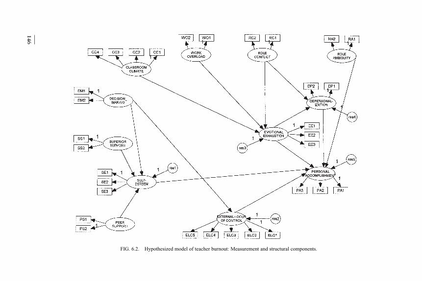
FIG. 6.2. Hypothesized model of teacher burnout: Measurement and structural components.

146


tant preliminary step in the analysis of full latent variable models is to test first forthe validity of the measurement model before making any attempt to evaluate thestructural model. Accordingly, CFA procedures are used in testing the validity ofthe indicator variables. Once it is known that the measurement model is operatingadequately,3 one can then have more confidence in findings related to the assess-ment of the hypothesized structural model.

In the present case, CFAs were conducted for indicator variables derived fromeach of the two multidimensional scales; these were the Teacher Stress Scale (TSS;Pettegrew & Wolf, 1982), which included all organizational indicator variablesexcept classroom climate, and the Maslach Burnout Inventory (MBI; Maslach &Jackson, 1986), measuring the three facets of burnout. The hypothesized CFAmodel of the TSS is portrayed in Fig. 6.4.

Of particular note here is the presence of double-headed arrows among all sixfactors. Recall from chapter 2 that, in contrast to AMOS Basic, AMOS Graphicsassumes no correlations among the factors. Thus, should you wish to estimate thesevalues in accordance with the related theory, they must be present in the model.Nonetheless, despite this requirement, AMOS Graphics will prompt you shouldyou neglect to include one or more factor correlations in the model. For example,

FIG. 6.3. AMOS Graphics: Inter-face Properties dialog box.

3For example, it may be that to attain a better fitting CFA model, the specification of a cross-load-ing is needed.

148 CHAPTER 6

FIG. 6.4. Hypothesized CFA model of the teacher stress scale.

Fig. 6.5 presents the error message triggered by my failure to include a correlationbetween Role Conflict (RoleC) and Decisionmaking (DecM).

Although goodness of fit for both the MBI (CFI = .98) and TSS (CFI = .97) wasfound to be exceptionally good, the solution for the TSS was somewhat problemat-ic. More specifically, an error message in the output warned that the covariancematrix among the factors was not positive definite; as a consequence, the solutionwas considered to be inadmissible. This message is shown in Table 6.1.

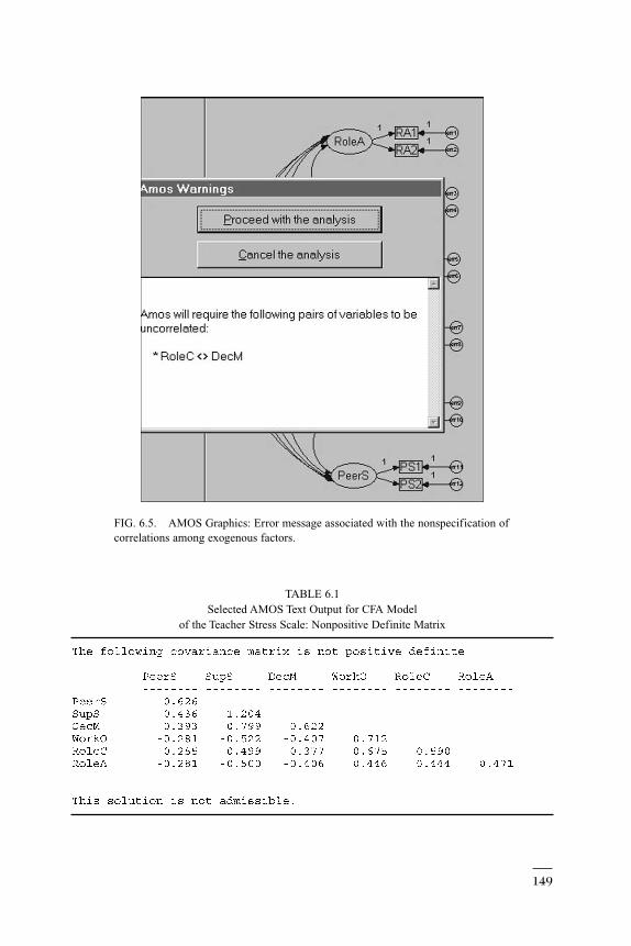
FIG. 6.5. AMOS Graphics: Error message associated with the nonspecification ofcorrelations among exogenous factors.

TABLE 6.1Selected AMOS Text Output for CFA Model

of the Teacher Stress Scale: Nonpositive Definite Matrix

149

150 CHAPTER 6

Multicollinearity is often the major contributing factor to the formulation of anonpositive definite matrix. This condition arises from the situation where two ormore variables are so highly correlated that they both, essentially, represent thesame underlying construct. Indeed, in checking out this possibility, I found the cor-relation between role conflict (RoleC) and work overload (WorkO) to be 1.041,which definitely signals a problem of multicollinearity. Substantively, this findingis not surprising as there appears to be substantial content overlap among TSSitems measuring role conflict and work overload. Of course, the very presence of acorrelation >1.00 is indicative of a solution that is clearly inadmissible. However,the flip side of the coin regarding inadmissible solutions is that they alert theresearcher to serious model misspecifications.

In an effort to address this problem of multicollinearity, a second CFA model ofthe TSS was specified in which the factor of work overload was deleted, but its twoobserved indicator variables were loaded onto the role conflict factor. Goodness of fitrelated to this five-factor model of the TSS (χ2

(44) = 152.37; CFI = .973; RMSEA =.064) was almost identical to the six-factor hypothesized model (χ2

(39) = 145.95; CFI= .973; RMSEA = .068). Furthermore, the factor covariance matrix was no longernonpositive definite. Thus, this five-factor structure served as the measurementmodel for the TSS throughout analyses related to the full causal model. However, asa consequence of this measurement restructuring, the revised model of burnoutshown in Fig. 6.6 replaced the originally hypothesized model (see Fig. 6.2) in serv-ing as the hypothesized model to be tested. Once again, in the interest of clarity, thefactor correlations and errors of measurement are not included.

AMOS Text Output: Hypothesized Model

Before examining the results of our testing of the hypothesized model, I considerit important to review, first, the status of all factors comprising this model. Turningto Table 6.2 we can see that there are five dependent factors in the model (deper-sonalization [DP], external locus of control [ELC], emotional exhaustion [EE],personal accomplishment [PA], self-esteem [SE]); each of these factors has single-headed arrows pointing at it, thereby easily identifying it as a dependent factor inthe model. The independent factors are those hypothesized as exerting an influenceon the dependent factors; these are role ambiguity (RA), role conflict (RC), deci-sion making (DM), superior support (SS), peer support (PS), and classroom cli-mate (CC). Additional information from this table informs us there are 599 cases,that the correct number of degrees of freedom is 436, and that the minimum wasachieved in reaching a convergent solution.

Model Assessment

Goodness-of-Fit Summary. Selected goodness-of-fit statistics related to thehypothesized model are presented in Table 6.3. Here, we see that the overall χ2

value, with 436 degrees of freedom, is 1030.892. Given the known sensitivity of

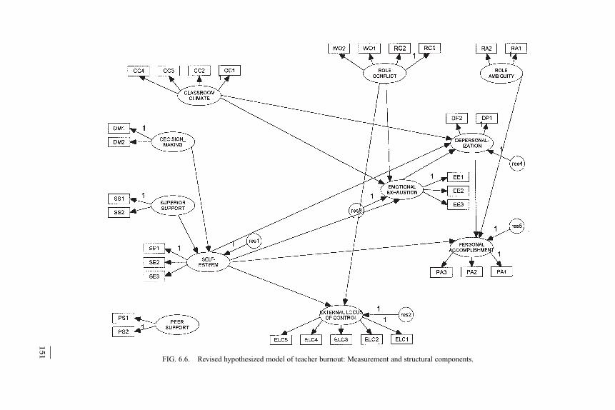
FIG. 6.6. Revised hypothesized model of teacher burnout: Measurement and structural components.

151

152 CHAPTER 6

this statistic to sample size, however, use of the χ2 index provides little guidance indetermining the extent to which the model does not fit. Thus, it is more beneficialto rely on other indexes of fit. Primary among these are the GFI, CFI, and RMSEA.Furthermore, given that we shall be comparing a series of models in our quest toobtain a final well-fitting model, the ECVI is also of interest.

Interestingly, although the GFI (.903) suggests that model fit was only margin-ally adequate, the CFI (.941) suggests that it is relatively well-fitting. In addition,the RMSEA value of .048 is well within the recommended range of acceptability(<.05 to .08). Finally, the ECVI value for this initially hypothesized model is 2.032.This value, as noted earlier in the book, has no substantive meaning; rather, it is

TABLE 6.2Selected AMOS Text Output for Hypothesized Model: Model Summary


used within a relative framework. (For a review of these rule-of-thumb guidelines,you may wish to consult chap. 3, where goodness-of-fit indexes are described inmore detail.)

Modification Indexes. Over and above the fit of the model as a whole, how-ever, a review of the modification indices reveals some evidence of misfit in themodel. Because we are interested solely in the causal paths of the model at thispoint, only a subset of indexes related to the regression weights is included in Table

TABLE 6.3Selected AMOS Output Text for Hypothesized Model: Goodness-of-Fit Statistics

154 CHAPTER 6

6.4. Turning to this table, you will note that the first 10 modification indexes (MIs)are enclosed in a rectangle. These parameters represent the structural (i.e., causal)paths in the model and are the only MIs of interest. Some of the remaining MIs inTable 6.4 represent the cross-loading of an indicator variable onto a factor otherthan the one it was designed to measure (EE3 ← CC). Others represent the regres-sion of one indicator variable on another; these MIs are substantively meaningless.4

In reviewing the information provided in the rectangle, note that the maximumMI is associated with the regression path flowing from classroom climate to deper-sonalization (DP ← CC). The value of 24.776 indicates that, if this parameter wereto be freely estimated in a subsequent model, the overall χ2 value would drop by atleast this amount. If you turn now to the expected parameter change statistic relat-ed to this parameter, you will find a value of −0.351; this value represents theapproximate value that the newly estimated parameter would assume.

In data preparation, the TSS items measuring classroom climate were reflectedsuch that low scores were indicative of a poor classroom milieu, and high scores, ofa good classroom milieu. From a substantive perspective, it would seem perfectly rea-sonable that elementary school teachers whose responses yielded low scores forclassroom climate should concomitantly display high levels of depersonalization.Given the meaningfulness of this influential flow, the model was reestimated with thepath from classroom climate to depersonalization specified as a free parameter; thismodel is subsequently labeled as Model 2. Results related to this respecified modelare discussed within the framework of post hoc analyses in the next section.

POST HOC ANALYSES

AMOS Text Output: Model 2

In the interest of space, only the final model of burnout, as determined from thefollowing post hoc model-fitting procedures, is displayed. However, relevant por-tions of the AMOS output, pertinent to each respecified model, are presented anddiscussed.

Model Assessment

Goodness-of-Fit Summary. The estimation of Model 2 yielded an overallχ2

(435) value of 995.019, a GFI of .906, a CFI of .945, and an RMSEA of .046; theECVI value was 1.975. Although the improvement in model fit for Model 2, com-pared with the originally hypothesized model, would appear to be trivial on thebasis of the GFI, CFI, and RMSEA values, the model difference nonetheless wasstatistically significant (∆χ2

(1) = 35.873). Moreover, the parameter estimate for the

4As previously noted, the present version of AMOS provides no mechanism for excluding MIs suchas these.

TABLE 6.4Selected AMOS Text Output for Hypothesized Model: Modification Indexes

155

156 CHAPTER 6

path from classroom climate to depersonalization was slightly higher than the onepredicted by the expected parameter change statistic (−0.479 vs. −0.351) and it wasstatistically significant (C.R. = −5.712). Modification indexes related to the struc-tural parameters for Model 2 are shown in Table 6.5.

TABLE 6.5Selected AMOS Text Output for Model 2: Modification Indexes


5Of course, had a nonrecursive model represented the hypothesized model, such feedback pathswould be of interest.

Modification Indexes. In reviewing the boxed statistics presented in Table6.5, we see that there are still nine MIs that can be taken into account in the deter-mination of a well-fitting model of burnout. The largest of these (MI = 20.311) isassociated with a path flowing from self-esteem to external locus of control (ELC← SE), and the expected value is estimated to be −0.184. Substantively, this pathagain makes good sense. Indeed, it seems likely that teachers who exhibit high lev-els of self-esteem also exhibit low levels of external locus of control. On the basisof this rationale, and despite the fact that the Expected Parameter Change statisticis larger for the DP ← SE path, we remain consistent in focusing on the path asso-ciated with the largest MI. (Recall Bentler’s 1995 caveat, noted in chap. 3, thatthese values can be affected by both the scaling and identification of factors andvariables.) Thus, the causal structure was again respecified—this time, with thepath from self-esteem to external locus of control freely estimated (Model 3).


Goodness-of-Fit Summary. Model 3 yielded an overall χ2(434) value of

967.244, with GFI = .909, CFI = .947, and RMSEA = .045; the ECVI was 1.932.Again, the χ2 difference between Model 2 and Model 3 was statistically significant(∆χ2

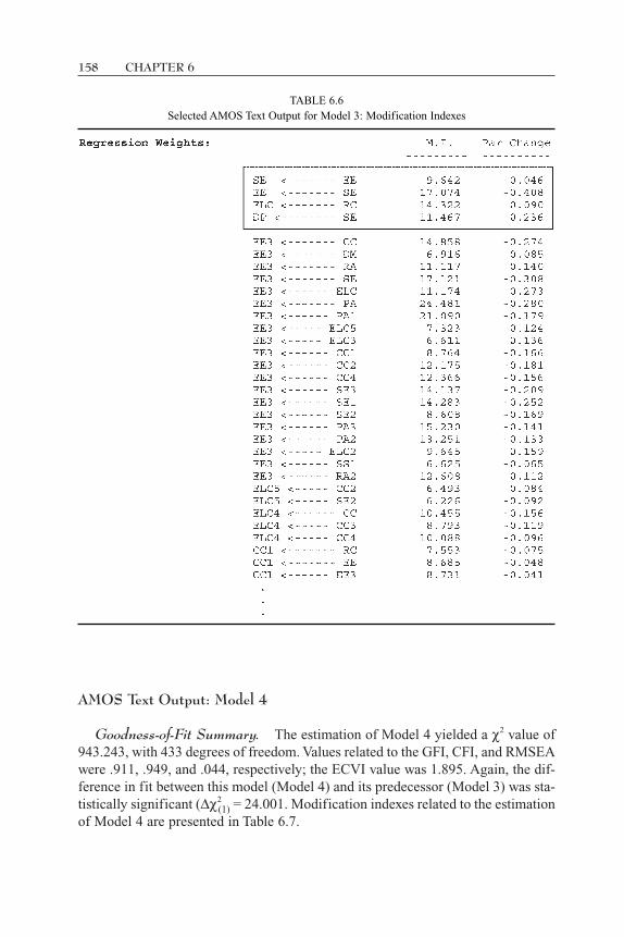
(1) = 27.775). Modification indexes related to Model 3 are shown in Table 6.6.Of initial import here is the fact that the number of MIs has now dropped from nineto only four. This discrepancy in the number of MI values between Model 2 andModel 3 serves as a perfect example of why the incorporation of additional param-eters into the model must be done one at a time.

Modification Indexes. Reviewing the boxed statistics here, we see that thelargest MI (17.074) is associated with a path from self-esteem to emotionalexhaustion (EE ← SE). However, it is important that you note that an MI (9.642)related to the reverse path involving these factors (SE ← EE) is also included asan MI. As emphasized in chapter 3, parameters identified by AMOS as belong-ing in a model are based on statistical criteria only; of more import is that theirinclusion be substantively meaningful. Within the context of the original study,the incorporation of this latter path (SE ← EE) into the model would make nosense whatsoever because its primary purpose was to validate the impact of orga-nizational and personality variables on burnout, and not the reverse. Thus, weignore this suggested model modification.5 Because it seems reasonable thatteachers who exhibit high levels of self-esteem may, concomitantly, exhibit lowlevels of emotional exhaustion, the model was reestimated once again, with thispath freely estimated (Model 4).

158 CHAPTER 6


Goodness-of-Fit Summary. The estimation of Model 4 yielded a χ2 value of943.243, with 433 degrees of freedom. Values related to the GFI, CFI, and RMSEAwere .911, .949, and .044, respectively; the ECVI value was 1.895. Again, the dif-ference in fit between this model (Model 4) and its predecessor (Model 3) was sta-tistically significant (∆χ2

(1) = 24.001. Modification indexes related to the estimationof Model 4 are presented in Table 6.7.



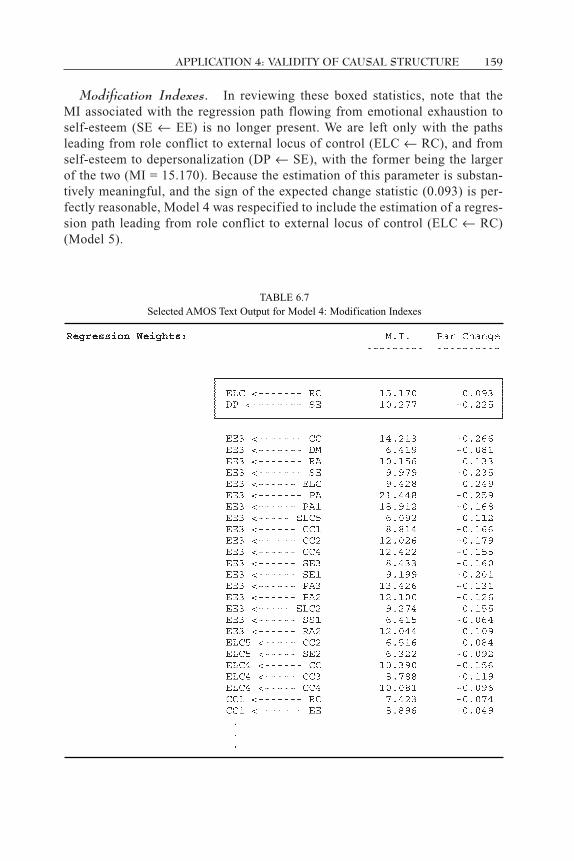
Modification Indexes. In reviewing these boxed statistics, note that theMI associated with the regression path flowing from emotional exhaustion toself-esteem (SE ← EE) is no longer present. We are left only with the pathsleading from role conflict to external locus of control (ELC ← RC), and fromself-esteem to depersonalization (DP ← SE), with the former being the largerof the two (MI = 15.170). Because the estimation of this parameter is substan-tively meaningful, and the sign of the expected change statistic (0.093) is per-fectly reasonable, Model 4 was respecified to include the estimation of a regres-sion path leading from role conflict to external locus of control (ELC ← RC)(Model 5).


160 CHAPTER 6


Goodness-of-Fit Summary. Results from the estimation of Model 5 yieldeda χ2

(432) value of 904.724, a GFI of .913, a CFI of .953, and an RMSEA of .043; theECVI value was 1.834. Again, the improvement in model fit was found to be sta-tistically significant (∆χ2

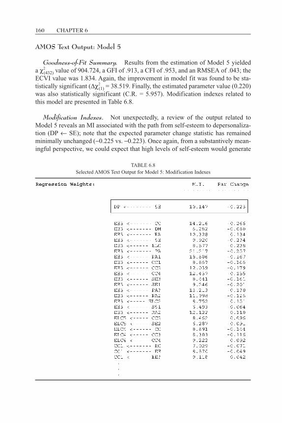
(1) = 38.519. Finally, the estimated parameter value (0.220)was also statistically significant (C.R. = 5.957). Modification indexes related tothis model are presented in Table 6.8.

Modification Indexes. Not unexpectedly, a review of the output related toModel 5 reveals an MI associated with the path from self-esteem to depersonaliza-tion (DP ← SE); note that the expected parameter change statistic has remainedminimally unchanged (−0.225 vs. −0.223). Once again, from a substantively mean-ingful perspective, we could expect that high levels of self-esteem would generate



low levels of depersonalization thereby yielding a negative expected parameterchange statistic value. Thus, Model 5 was respecified with the path (DP ← SE)freely estimated, and was labeled as Model 6.


Goodness-of-Fit Summary. Estimation of Model 6 yielded an overall χ2(431)

value of 890.619; again, the χ2 difference between Models 3 and 4 was statistical-ly significant (∆χ2

(1) = 14.105), as was the estimated parameter (−0.310, C.R. = −3.766). Furthermore, there was virtually no change in the GFI (.913), CFI (.953),and RMSEA (.043) values; the ECVI dropped a little further to 1.814, thereby indi-cating that Model 6 represented the best fit to the data thus far in the analyses. Asexpected, and as can be seen in Table 6.9, no MIs associated with structural pathswere present in the output; only MIs related to the regression weights of factorloadings were presented. As you will note, there are no outstanding values sugges-tive of model misfit. Taking each of these factors into account, no further consid-eration was given to the inclusion of additional parameters.

Model Parsimony. Thus far, discussion related to model fit has consideredonly the addition of parameters to the model. However, another side to the questionof fit, particularly as it pertains to a full model, is the extent to which certain ini-tially hypothesized paths may be irrelevant to the model. One way of determiningsuch irrelevancy is to examine the statistical significance of all structural parame-ter estimates. This information, as derived from the estimation of Model 6, is pre-sented in Table 6.10.

In reviewing the structural parameter estimates for Model 6, we can see fiveparameters that are nonsignificant; these parameters represent the paths from peersupport to self-esteem (SE ← PS; C.R. = −0.595); role conflict to depersonaliza-tion (DP ← RC; C.R. = −0.839); decision making to external locus of control (ELC← DM; −1.400); emotional exhaustion to personal accomplishment (PA ← EE;


162 CHAPTER 6

−1.773); external locus of control to personal accomplishment (PA ← ELC; −0.895). In the interest of parsimony, a final model of burnout was estimated withthese five structural paths deleted from the model.

Because standardized estimates are typically of interest in presenting resultsfrom structural equation models, it is usually of interest to request these statisticswhen you have determined your final model. Given that Model 7 will serve as ourfinal model of teacher burnout, this request was made by clicking on the AnalysisProperties icon, which, in turn, yielded the dialog box shown in Fig. 6.7; youobserve that I also requested the squared multiple correlations.


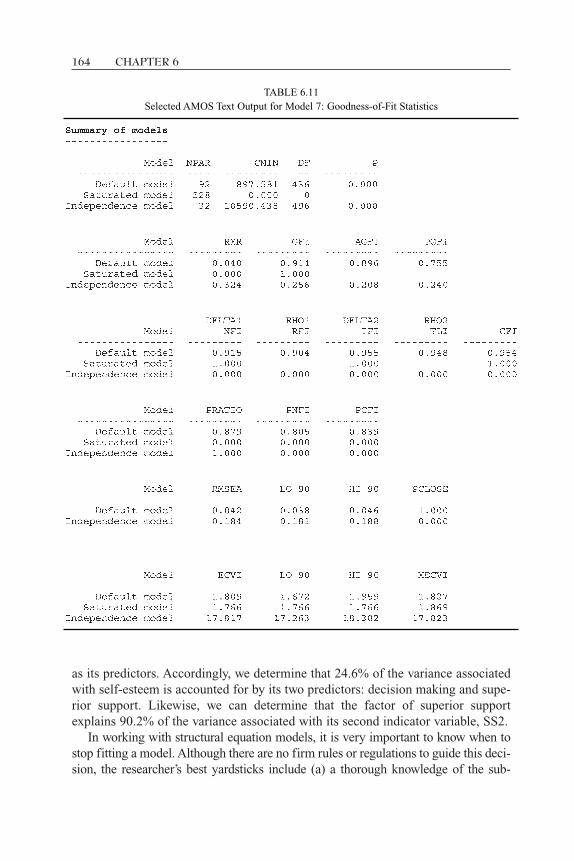
Goodness-of-Fit Summary. Estimation of this final model (Model 7) result-ed in an overall χ2

(436) value of 897.581. At this point, you may have some concernover the slight erosion in model fit from χ2

(431) = 890.619 for Model 4, to χ2(436) =

897.581 for Model 7, the final model. However, with deletion of any parametersfrom a model, such a change is to be expected. The important aspect of this changein model fit is that the χ2 difference between the two models is not significant(∆χ2

(5) = 6.962). Furthermore, from a review of the goodness-of-fit statistics inTable 6.11, you will note that values for the other fit indexes of interest remainedvirtually unchanged from those related to Model 6 (GFI = .914; CFI = .954;RMSEA = .042); the slight drop in the ECVI value signals that this final and mostparsimonious model represents the best fit to the data overall.

TABLE 6.10Selected AMOS Text Output for Model 6: Maximum Likelihood Estimates for Structural Paths


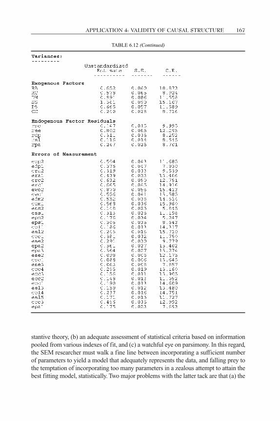
A schematic representation of this final model of burnout for elementary teach-ers is displayed in Fig. 6.8, and the unstandardized, as well as standardized, maxi-mum likelihood parameter estimates are presented in Table 6.12. It is important todraw your attention to the fact that all parameter estimates are statistically signifi-cant and substantively meaningful.

Taking one last look at this final model of burnout, let’s review the squared mul-tiple correlations (SMCs) shown in Table 6.13. The SMC is a useful statistic that isindependent of all units of measurement. Once it is requested, AMOS 4.0 will pro-vide a SMC for each endogenous variable in the model. Thus, in Table 6.13, yousee SMCs for the dependent factors in the model (SE, EE, DP, PA, ELC) and foreach of the factor loading regression paths (CC1–SS2). The SMC value representsthe proportion of variance that is explained by the predictors of the variable inquestion. For example, in order to interpret the SMC associated with self-esteem(SE), we need first to review Fig. 6.8 to ascertain which factors in the model serve

FIG. 6.7. AMOS Graphics: Analysis Properties dialog box.

164 CHAPTER 6

as its predictors. Accordingly, we determine that 24.6% of the variance associatedwith self-esteem is accounted for by its two predictors: decision making and supe-rior support. Likewise, we can determine that the factor of superior supportexplains 90.2% of the variance associated with its second indicator variable, SS2.

In working with structural equation models, it is very important to know when tostop fitting a model. Although there are no firm rules or regulations to guide this deci-sion, the researcher’s best yardsticks include (a) a thorough knowledge of the sub-

TABLE 6.11Selected AMOS Text Output for Model 7: Goodness-of-Fit Statistics

FIG. 6.8. Final model of burnout for elementary school teachers.

165

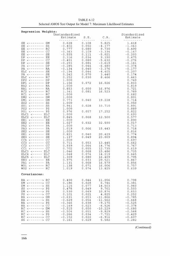
TABLE 6.12Selected AMOS Text Output for Model 7: Maximum Likelihood Estimates

(Continued)

166


stantive theory, (b) an adequate assessment of statistical criteria based on informationpooled from various indexes of fit, and (c) a watchful eye on parsimony. In this regard,the SEM researcher must walk a fine line between incorporating a sufficient numberof parameters to yield a model that adequately represents the data, and falling prey tothe temptation of incorporating too many parameters in a zealous attempt to attain thebest fitting model, statistically. Two major problems with the latter tack are that (a) the

TABLE 6.12 (Continued)

168 CHAPTER 6

model can comprise parameters that actually contribute only trivially to its structure,and (b) the more parameters there are in a model, the more difficult it is to replicateits structure should future validation research be conducted.

In the case of the model tested in this chapter, I considered the addition of fivestructural paths to be justified both substantively and statistically. From the statis-tical perspective, it was noted that the addition of each new parameter resulted in astatistically significant difference in fit from the previously specified model. Theinclusion of these five additional paths, and the deletion of five originally specifiedpaths, resulted in a final model that fitted the data well (GFI = .914; CFI = .954;RMSEA = .042). Furthermore, based on the ECVI index, it appears that the final

TABLE 6.13Selected AMOS Text Output for Model 7: Squared Multiple Correlations


model (Model 7) has the greatest potential for replication in other samples of ele-mentary teachers, compared with Models 1 through 6.

In concluding this chapter, let’s now summarize and review findings from the var-ious models tested. First, of 13 causal paths specified in the revised hypothesizedmodel (see Fig. 6.6), 8 were found to be statistically significant for elementary teach-ers. These paths reflected the impact of (a) classroom climate and role conflict onemotional exhaustion, (b) decision making and superior support on self-esteem, (c)self-esteem, role ambiguity, and depersonalization on perceived personal accom-plishment, and (d) emotional exhaustion on depersonalization. Second, five paths,not specified a priori (classroom climate → depersonalization; self-esteem → exter-nal locus of control; self-esteem → emotional exhaustion; role conflict → externallocus of control; self-esteem → depersonalization), proved to be essential compo-nents of the causal structure; they were therefore added to the model. Finally, fivehypothesized paths (peer support → self-esteem; role conflict → depersonalization;decision making → external locus of control; emotional exhaustion → personalaccomplishment; external locus of control → personal accomplishment) were notsignificant and were subsequently deleted from the model.

In general, we can conclude from this application that role ambiguity, role con-flict, classroom climate, participation in the decision-making process, and the sup-port of one’s superiors are potent organizational determinants of burnout for ele-mentary school teachers. The process, however, appears to be strongly tempered byones sense of self-worth.

MODELING WITH AMOS BASIC

For an example of an AMOS Basic file in this chapter, let’s examine one related tothe final model of burnout schematically displayed in Fig. 6.8. This input file ispresented in Table 6.14.

Although most of the setup here will be familiar to you at this point, a couple ofpoints are perhaps worthy of comment. First, note that the first three SEM linesrequest that the output be in text format, and that both the squared multiple correla-tions and the standardized estimates be included. The fourth SEM line identifies thefile “elind1l.txt” as the data source. Second, for purposes of clarity, I have separatedequations related to the measurement model (RA1–PA3) from those representing thestructural model. Finally, I wish to point out that, although I have located the paren-thesized values of 1, representing constrained parameters to precede the parameter inquestion, these values can also follow the related parameter; preference related to thisspecification in the structuring of an AMOS Basic input file is purely arbitrary.

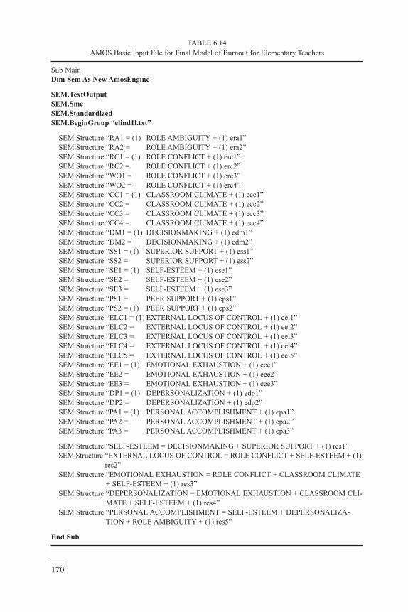
TABLE 6.14 AMOS Basic Input File for Final Model of Burnout for Elementary Teachers

Sub MainDim Sem As New AmosEngine

SEM.TextOutputSEM.SmcSEM.StandardizedSEM.BeginGroup “elind1l.txt”

SEM.Structure “RA1 = (1) ROLE AMBIGUITY + (1) era1”SEM.Structure “RA2 = ROLE AMBIGUITY + (1) era2”SEM.Structure “RC1 = (1) ROLE CONFLICT + (1) erc1”SEM.Structure “RC2 = ROLE CONFLICT + (1) erc2”SEM.Structure “WO1 = ROLE CONFLICT + (1) erc3”SEM.Structure “WO2 = ROLE CONFLICT + (1) erc4”SEM.Structure “CC1 = (1) CLASSROOM CLIMATE + (1) ecc1”SEM.Structure “CC2 = CLASSROOM CLIMATE + (1) ecc2”SEM.Structure “CC3 = CLASSROOM CLIMATE + (1) ecc3”SEM.Structure “CC4 = CLASSROOM CLIMATE + (1) ecc4”SEM.Structure “DM1 = (1) DECISIONMAKING + (1) edm1”SEM.Structure “DM2 = DECISIONMAKING + (1) edm2”SEM.Structure “SS1 = (1) SUPERIOR SUPPORT + (1) ess1”SEM.Structure “SS2 = SUPERIOR SUPPORT + (1) ess2”SEM.Structure “SE1 = (1) SELF-ESTEEM + (1) ese1”SEM.Structure “SE2 = SELF-ESTEEM + (1) ese2”SEM.Structure “SE3 = SELF-ESTEEM + (1) ese3”SEM.Structure “PS1 = PEER SUPPORT + (1) eps1”SEM.Structure “PS2 = (1) PEER SUPPORT + (1) eps2”SEM.Structure “ELC1 = (1) EXTERNAL LOCUS OF CONTROL + (1) eel1”SEM.Structure “ELC2 = EXTERNAL LOCUS OF CONTROL + (1) eel2”SEM.Structure “ELC3 = EXTERNAL LOCUS OF CONTROL + (1) eel3”SEM.Structure “ELC4 = EXTERNAL LOCUS OF CONTROL + (1) eel4”SEM.Structure “ELC5 = EXTERNAL LOCUS OF CONTROL + (1) eel5”SEM.Structure “EE1 = (1) EMOTIONAL EXHAUSTION + (1) eee1”SEM.Structure “EE2 = EMOTIONAL EXHAUSTION + (1) eee2”SEM.Structure “EE3 = EMOTIONAL EXHAUSTION + (1) eee3”SEM.Structure “DP1 = (1) DEPERSONALIZATION + (1) edp1”SEM.Structure “DP2 = DEPERSONALIZATION + (1) edp2”SEM.Structure “PA1 = (1) PERSONAL ACCOMPLISHMENT + (1) epa1”SEM.Structure “PA2 = PERSONAL ACCOMPLISHMENT + (1) epa2”SEM.Structure “PA3 = PERSONAL ACCOMPLISHMENT + (1) epa3”

SEM.Structure “SELF-ESTEEM = DECISIONMAKING + SUPERIOR SUPPORT + (1) res1”SEM.Structure “EXTERNAL LOCUS OF CONTROL = ROLE CONFLICT + SELF-ESTEEM + (1)

res2”SEM.Structure “EMOTIONAL EXHAUSTION = ROLE CONFLICT + CLASSROOM CLIMATE

+ SELF-ESTEEM + (1) res3”SEM.Structure “DEPERSONALIZATION = EMOTIONAL EXHAUSTION + CLASSROOM CLI-

MATE + SELF-ESTEEM + (1) res4”SEM.Structure “PERSONAL ACCOMPLISHMENT = SELF-ESTEEM + DEPERSONALIZA-

TION + ROLE AMBIGUITY + (1) res5”

End Sub

170

Testing for the Validity of a Causal Structure - SPSS · Testing for the Validity of a Causal...

Documents

Transcript of Testing for the Validity of a Causal Structure - SPSS · Testing for the Validity of a Causal...