Testing Closeness of Discrete...

Testing Closeness of Discrete Distributions

TUGKAN BATU

London School of Economics and Political Science

LANCE FORTNOW

Northwestern University

RONITT RUBINFELD

Massachusetts Institute of Technology and Tel Aviv University

WARREN D. SMITH

Center for Range Voting

and

PATRICK WHITE

Given samples from two distributions over an n-element set, we wish to test whether these dis-tributions are statistically close. We present an algorithm which uses sublinear in n, specifically,O(n2/3ǫ−8/3 log n), independent samples from each distribution, runs in time linear in the samplesize, makes no assumptions about the structure of the distributions, and distinguishes the caseswhen the distance between the distributions is small (less than maxǫ4/3n−1/3/32, ǫn−1/2/4) orlarge (more than ǫ) in ℓ1 distance. This result can be compared to the lower bound of Ω(n2/3ǫ−2/3)for this problem given by Valiant [2008].

Our algorithm has applications to the problem of testing whether a given Markov process israpidly mixing. We present sublinear algorithms for several variants of this problem as well.

Categories and Subject Descriptors: F.2.2 [Analysis of Algorithms and Problem Complex-ity]: Nonnumerical Algorithms and Problems; G.3 [Probability and Statistics]: StatisticalComputing

General Terms: Algorithms, Theory

Additional Key Words and Phrases: Testing properties of distributions, statistical distance, testingMarkov chains for mixing

A preliminary version of this paper [Batu et al. 2000] appeared in the 41st Symposium onFoundations of Computer Science, 2000, Redondo Beach, CA.T. Batu, Department of Mathematics, London School of Economics and Political Science,London, UK. Email: [email protected]. Fortnow, Department of Electrical Engineering and Computer Science, Northwestern Univer-sity, Chicago, IL, USA. Email: [email protected]. Research done while at NECResearch Institute.R. Rubinfeld, CSAIL, MIT, Cambridge, MA, USA and the Blavatnik School of ComputerScience, Tel Aviv University. Email: [email protected]. Research done while at NEC Research

Institute.W.D. Smith, 21 Shore Oaks Drive, Stony Brook, NY, USA. Email: [email protected] done while at NEC Research Institute.

Permission to make digital/hard copy of all or part of this material without fee for personalor classroom use provided that the copies are not made or distributed for profit or commercialadvantage, the ACM copyright/server notice, the title of the publication, and its date appear, andnotice is given that copying is by permission of the ACM, Inc. To copy otherwise, to republish,to post on servers, or to redistribute to lists requires prior specific permission and/or a fee.c© 20YY ACM 0004-5411/20YY/0100-0001 $5.00

Journal of the ACM, Vol. V, No. N, Month 20YY, Pages 1–0??.

2 · Tugkan Batu et al.

1. INTRODUCTION

Suppose we have two distributions over the same n-element set, such that we knownothing about their structure and the only access we have to these distributions isthe ability to take independent samples from them. Suppose further that we wantto know whether these two distributions are close to each other in ℓ1 norm.1 Afirst approach, which we refer to as the naive approach, would be to sample enoughelements from each distribution so that we can approximate the distribution andthen compare the approximations. It is easy to see (see Theorem 3.11 in Section 3.2)that this naive approach requires the number of samples to be at least linear in n.

In this paper, we develop a method of testing that the distance between twodistributions is at most ǫ using considerably fewer samples. If the distributionshave ℓ1 distance at most maxǫ4/3n−1/3/32, ǫn−1/2/4, then the algorithm willaccept with probability at least 1 − δ. If the distributions have ℓ1 distance morethan ǫ then the algorithm will accept with probability at most δ. The number ofsamples used is O(n2/3ǫ−8/3 log(n/δ)). In contrast, the methods of Valiant [2008],fixing the incomplete arguments in the original conference paper (see Section 3),yield an Ω(n2/3ǫ−2/3) lower bound for testing ℓ1 distance in this model.

Our test relies on a test for whether two distributions have small ℓ2 distance,which is considerably easier to test: we give an algorithm with sample complexityindependent of n. However, small ℓ2 distance does not in general give a goodmeasure of the closeness of two distributions according to ℓ1 distance. For example,two distributions can have disjoint support and still have ℓ2 distance of O(1/

√n).

Still, we can get a very good estimate of the ℓ2 distance, say to within O(1/√

n)additive error, and then use the fact that the ℓ1 distance is at most

√n times the

ℓ2 distance. Unfortunately, the number of queries required by this approach is toolarge in general. Because of this, our ℓ1 test is forced to distinguish between twocases.

For distributions with small ℓ2 norm, we show how to use the ℓ2 distance to get anefficient test for ℓ1 distance. For distributions with larger ℓ2 norm, we use the factthat such distributions must have elements which occur with relatively high proba-bility. We create a filtering test that partitions the domain into those elements withrelatively high probability and all the other elements (those with relatively low prob-ability). The test estimates the ℓ1 distance due to these high-probability elementsdirectly, using the naive approach mentioned above. The test then approximatesthe ℓ1 distance due to the low-probability elements using the test for ℓ2 distance.Optimizing the notion of “high probability” yields our O(n2/3ǫ−8/3 log(n/δ)) algo-rithm. The ℓ2 distance test uses O(ǫ−4 log(1/δ)) samples.

Applying our techniques to Markov chains, we use the above algorithm as a basisfor constructing tests for determining whether a Markov chain is rapidly mixing.We show how to test whether iterating a Markov chain for t steps causes it to reacha distribution close to the stationary distribution. Our testing algorithm works byfollowing O(tn5/3) edges in the chain. When the Markov chain is dense enoughand represented in a convenient way (such a representation can be computed inlinear time and we give an example representation in Section 4), this test remains

1Half of ℓ1 distance between two distributions is also referred to as total variation distance.

Journal of the ACM, Vol. V, No. N, Month 20YY.

Testing Closeness of Discrete Distributions · 3

sublinear in the size of the Markov chain for small t. We then investigate two notionsof being close to a rapidly mixing Markov chain that fall within the framework ofproperty testing, and show how to test that a given Markov chain is close to aMarkov chain that mixes in t steps by following only O(tn2/3) edges. In the caseof Markov chains that come from directed graphs and pass our test, our theoremsshow the existence of a directed graph that is both close to the original one andrapidly mixing.

1.1 Related Work

1.1.1 Testing Properties of Distributions. The use of collision statistics in asample has been proposed as a technique to test whether a distribution is uniform(see, for example, Knuth [1973]). Goldreich and Ron [2000] give the first formalanalysis that using O(

√n) samples to estimate the collision probability yields an

algorithm which gives a very good estimate of the ℓ2 distance between the givendistribution and the uniform distribution. Their “collision count” idea underlies thepresent paper. More recently, Paninski [2008] presents a test to determine whethera distribution is far from the uniform distribution with respect to ℓ1 distance us-ing Θ(

√n/ǫ2) samples. Ma [1981] also uses collisions to measure the entropy of a

distribution defined by particle trajectories. After the publication of the prelimi-nary version of this paper, a long line of publications appeared regarding testingproperties of distributions including independence, entropy, and monotonicity (see,for example, [Batu et al. 2001; Batu et al. 2004; Batu et al. 2005; Brautbar andSamorodnitsky 2007; Alon et al. 2007; Valiant 2008; Rubinfeld and Servedio 2009;Raskhodnikova et al. 2009; Rubinfeld and Xie 2010; Adamaszek et al. 2010]).

1.1.2 Expansion, Rapid Mixing, and Conductance. Goldreich and Ron [2000]present a test that they conjecture can be used to give an algorithm with O(

√n)

query complexity which tests whether a regular graph is close to being an expander,where by close they mean that by changing a small fraction of the edges theycan turn it into an expander. Their test is based on picking a random node andtesting whether random walks from this node reach a distribution that is close tothe uniform distribution on the nodes. Our tests for Markov chains are based onsimilar principles. Mixing and expansion are known to be related [Sinclair andJerrum 1989], but our techniques only apply to the mixing properties of randomwalks on directed graphs, since the notion of closeness we use does not preservethe symmetry of the adjacency matrix. More recently, a series of papers [Czumajand Sohler 2007; Kale and Seshadhri 2008; Nachmias and Shapira 2007] answerGoldreich and Ron’s conjecture in the affirmative. In a previous work, Goldreichand Ron [1997] show that testing that a graph is close to an expander requiresΩ(n1/2) queries.

The conductance [Sinclair and Jerrum 1989] of a graph is known to be closely re-lated to expansion and rapid-mixing properties of the graph [Kannan 1994; Sinclairand Jerrum 1989]. Frieze and Kannan [1999] show, given a graph G with n verticesand α, one can approximate the conductance of G to within additive error α in

time n ·2O(1/α2). Their techniques also yield an 2poly(1/ǫ)-time test that determineswhether the adjacency matrix of a graph can be changed in at most ǫ fraction of thelocations to get a graph with high conductance. However, for the purpose of testing



whether an n-vertex, m-edge graph is rapid mixing, we would need to approximateits conductance to within α = O(m/n2); thus, only when m = Θ(n2), would thealgorithm in [Frieze and Kannan 1999] run in O(n) time.

We now discuss some other known results for testing of rapid mixing througheigenvalue computations. It is known that mixing [Sinclair and Jerrum 1989; Kan-nan 1994] is related to the separation between the two largest eigenvalues [Alon1986]. Standard techniques for approximating the eigenvalues of a dense n × nmatrix run in Θ(n3) floating-point operations and consume Θ(n2) words of mem-ory [Golub and van Loan 1996]. However, for a sparse n × n symmetric matrixwith m nonzero entries, n ≤ m, “Lanczos algorithms” [Parlett 1998] accomplishthe same task in Θ(n(m + log n)) floating-point operations, consuming Θ(n + m)storage. Furthermore, it is found in practice that these algorithms can be run forfar fewer, even a constant number, of iterations while still obtaining highly accuratevalues for the outer and inner few eigenvalues.

1.1.3 Streaming. There is much work on the problem estimating the distancebetween distributions in data streaming models where space rather than time islimited (cf., [Gibbons and Matias 1999; Alon et al. 1999; Feigenbaum et al. 1999;Fong and Strauss 2000]). Another line of work [Broder et al. 2000] estimates the dis-tance in frequency count distributions on words between various documents, whereagain space is limited. Guha et al. [2009] have extended our result to estimatingthe closeness of distribution with respect to a range of f -divergences, which includeℓ1 distance. Testing distributions in streaming data models has been an active areaof research in the recent years (see, for example, [Bhuvanagiri and Ganguly 2006;Chakrabarti et al. 2006; Indyk and McGregor 2008; Guha et al. 2008; Chakrabartiet al. 2010; Chien et al. 2010; Braverman and Ostrovsky 2010a; 2010b]).

1.1.4 Other Related Models. In an interactive setting, Sahai and Vadhan [1997]show that, given distributions p and q generated by polynomial-size circuits, theproblem of distinguishing whether p and q are close or far in ℓ1 norm is completefor statistical zero knowledge. Kannan and Yao [1991] outlines a program checkingframework for certifying the randomness of a program’s output. In their model,one does not assume that samples from the input distribution are independent.

1.1.5 Computational Learning Theory. There is a vast literature on testing sta-tistical hypotheses. In these works, one is given examples chosen from the samedistribution out of two possible choices, say p and q. The goal is to decide whichof two distributions the examples are coming from. More generally, the goal canbe stated as deciding which of two known classes of distributions contains the dis-tribution generating the examples. This can be seen to be a generalization of ourmodel as follows: Let the first class of distributions be the set of distributions ofthe form q × q. Let the second class of distributions be the set of distributions ofthe form q1 × q2 where the ℓ1 difference of q1 and q2 is at least ǫ. Then, givenexamples from two distributions p1,p2, create a set of example pairs (x, y) wherex is chosen according to p1 and y according to p2 independently. Bounds and anoptimal algorithm for the general problem for various distance measures are givenin [Cover and Thomas 1991; Neyman and Pearson 1933; Cressie and Morgan 1989;Csiszar 1967; Lehmann 1986]. None of these give sublinear bounds in the domain



size for our problem. The specific model of singleton hypothesis classes is studiedby Yamanishi [1995].

1.2 Notation

We use the following notation. We denote the set 1, . . . , n with [n]. The notationx ∈R [n] denotes that x is chosen uniformly at random from the set [n]. The ℓ1

norm of a vector v is denoted by ‖v‖1 and is equal to∑n

i=1 |vi|. Similarly, the ℓ2

norm is denoted by ‖v‖2 and is equal to√∑n

i=1 v2i , and ‖v‖∞ = maxi |vi|. We

assume our distributions are discrete distributions over n elements, with labels in[n], and will represent such a distribution as a vector p = (p1, . . . , pn), where pi isthe probability of outputting element i.

The collision probability of two distributions p and q is the probability that asample from each of p and q yields the same element. Note that, for two distribu-tions p,q, the collision probability is p · q =

∑i piqi. To avoid ambiguity, we refer

to the collision probability of p and p as the self-collision probability of p. Notethat the self-collision probability of p is ‖p‖2

2.

2. TESTING CLOSENESS OF DISTRIBUTIONS

The main goal of this section is to show how to test whether two distributionsp and q are close in ℓ1 norm in sublinear time in the size of the domain of thedistributions. We are given access to these distributions via black boxes whichupon a query respond with an element of [n] generated according to the respectivedistribution. Our main theorem is:

Theorem 2.1. Given parameters δ and ǫ, and distributions p,q over a set ofn elements, there is a test which runs in time O(n2/3ǫ−8/3 log(n/δ)) such that, if

‖p− q‖1 ≤ max( ǫ4/3

32 3√

n, ǫ

4√

n), then the test accepts with probability at least 1 − δ

and, if ‖p− q‖1 > ǫ, then the test rejects with probability at least 1 − δ.

In order to prove this theorem, we give a test which determines whether p and q

are close in ℓ2 norm. The test is based on estimating the self-collision and collisionprobabilities of p and q. In particular, if p and q are close, one would expect thatthe self-collision probabilities of each are close to the collision probability of thepair. Formalizing this intuition, in Section 2.1, we prove:

Theorem 2.2. Given parameter δ and ǫ, and distributions p and q over a set ofn elements, there exists a test such that, if ‖p−q‖2 ≤ ǫ/2, then the test accepts withprobability at least 1 − δ and, if ‖p− q‖2 > ǫ, then the test rejects with probabilityat least 1 − δ. The running time of the test is O(ǫ−4 log(1/δ)).

The test used to prove Theorem 2.2 is given below in Figure 1. The number ofpairwise self-collisions in multiset F ⊆ [n] is the count of i < j such that the ithsample in F is same as the jth sample in F . Similarly, the number of collisionsbetween Qp ⊆ [n] and Qq ⊆ [n] is the count of (i, j) such that the ith sample in Qp

is same as the jth sample in Qq.We use the parameter m to indicate the number of samples needed by the test

to get constant confidence. In order to bound the ℓ2 distance between p and q

by ǫ, setting m = O( 1ǫ4 ) suffices. By maintaining arrays which count the numbers



ℓ2-Distance-Test(p, q, m, ǫ, δ)Repeat O(log(1/δ)) times

(1) Let Fp and Fq be multisets of m samples from p and q, respectively. Let rp and rq bethe numbers of pairwise self-collisions in Fp and Fq, respectively.

(2) Let Qp and Qq be multisets of m samples from p and q, respectively. Let spq bethe number of collisions between Qp and Qq.

(3) Let r = 2mm−1

(rp + rq). Let s = 2spq.

(4) If r − s > 3m2ǫ2/4, then reject the current iteration.

Reject if the majority of iterations reject, accept otherwise.

Fig. 1. Algorithm ℓ2-Distance-Test

of times, for example, Np(i) for Fp, that each element i is sampled and summing(Np(i)

2

)over all sampled i in the domain, one can achieve the claimed running

time bounds for computing an estimate of the collision probability. In this way,essentially m2 estimations of the collision probability can be performed in O(m)time.

Since ‖v‖1 ≤ √n · ‖v‖2, a simple way to extend the above test to an L1 distance

test is by setting ǫ′ = ǫ/√

n. This would give the correct output behavior for thetester. Unfortunately, due to the order of the dependence on ǫ in the ℓ2 distancetest, the resulting running time is quadratic in n. It is possible, though, to achievesublinear running times if the input distributions are known to be reasonably evenlydistributed. We make this precise by a closer analysis of the variance of the esti-mator in the test in Lemma 2.5. In particular, we analyze the dependence of thevariances of s and r on the parameter b = max(‖p‖∞, ‖q‖∞). There we show thatgiven p and q such that b = O(n−α), one can call ℓ2-Distance-Test with an errorparameter of ǫ√

nand achieve running time of O(ǫ−4(n1−α/2 +n2−2α)). Thus, when

the maximum probability of any element is bounded, the ℓ2 distance test can infact yield a sublinear-time algorithm for testing closeness in L1 distance.

In the previous paragraph, we have noted that, for distributions with a bound onthe maximum probability of any element, it is possible to test closeness with timeand queries sublinear in the domain size. On the other hand, when the minimumprobability element is quite large, the naive approach that we referred to in theintroduction can be significantly more efficient. This suggests a filtering algorithm,which separates the domain of the distributions being tested into two parts – thebig elements, or those elements to which the distributions assign relatively highprobability weight, and the small elements, which are all other elements. Then,the naive tester is applied to the distributions restricted to the big elements, andthe tester that is based on estimating the ℓ2 distance is applied to the distributionsrestricted to the small elements.

More specifically, we use the following definition to identify the elements withlarge weights.

Definition 2.3 Big element. An element i is called big with respect to a distribu-tion p if pi > (ǫ/n)2/3.

The complete test is given below in Figure 2. The proof of Theorem 2.1 is presentedin Section 2.2.



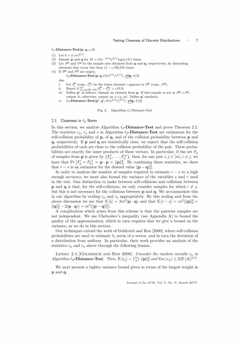
ℓ1-Distance-Test(p,q, ǫ, δ)

(1) Let b = (ǫ/n)2/3.(2) Sample p and q for M = O(ǫ−8/3n2/3 log(n/δ)) times.(3) Let Sp and Sq be the sample sets obtained from p and q, respectively, by discarding

elements that occur less than (1 − ǫ/26)Mb times.(4) If Sp and Sq are empty,

ℓ2-Distance-Test(p, q, O(n2/3/ǫ8/3), ǫ2√

n, δ/2)

elsei. Let ℓpi (resp., ℓqi ) be the times element i appears in Sp (resp., Sq).ii. Reject if

P

i∈Sp∪Sq |ℓpi − ℓqi | > ǫM/8.iii. Define p′ as follows: Sample an element from p. If this sample is not in Sp ∪ Sq,

output it; otherwise, output an x ∈R [n]. Define q′ similarly.iv. ℓ2-Distance-Test(p′, q′, O(n2/3/ǫ8/3), ǫ

2√

n, δ/2)

Fig. 2. Algorithm ℓ1-Distance-Test

2.1 Closeness in ℓ2 Norm

In this section, we analyze Algorithm ℓ2-Distance-Test and prove Theorem 2.2.The statistics rp, rq and s in Algorithm ℓ2-Distance-Test are estimators for theself-collision probability of p, of q, and of the collision probability between p andq, respectively. If p and q are statistically close, we expect that the self-collisionprobabilities of each are close to the collision probability of the pair. These proba-bilities are exactly the inner products of these vectors. In particular, if the set Fp

of samples from p is given by F 1p , . . . , Fm

p , then, for any pair i, j ∈ [m], i 6= j, we

have that Pr[F i

p = F jp

]= p · p = ‖p‖2

2. By combining these statistics, we showthat r − s is an estimator for the desired value ‖p− q‖2

2.In order to analyze the number of samples required to estimate r − s to a high

enough accuracy, we must also bound the variance of the variables s and r usedin the test. One distinction to make between self-collisions and collisions betweenp and q is that, for the self-collisions, we only consider samples for which i 6= j,but this is not necessary for the collisions between p and q. We accommodate thisin our algorithm by scaling rp and rq appropriately. By this scaling and from theabove discussion we see that E [s] = 2m2(p · q) and that E [r − s] = m2(‖p‖2

2 +‖q‖2

2 − 2(p · q)) = m2(‖p− q‖22).

A complication which arises from this scheme is that the pairwise samples arenot independent. We use Chebyshev’s inequality (see Appendix A) to bound thequality of the approximation, which in turn requires that we give a bound on thevariance, as we do in this section.

Our techniques extend the work of Goldreich and Ron [2000], where self-collisionprobabilities are used to estimate ℓ2 norm of a vector, and in turn the deviation ofa distribution from uniform. In particular, their work provides an analysis of thestatistics rp and rq above through the following lemma.

Lemma 2.4 [Goldreich and Ron 2000]. Consider the random variable rp inAlgorithm ℓ2-Distance-Test. Then, E [rp] =

(m2

)·‖p‖2

2 and Var (rp) ≤ 2(E [A])3/2.

We next present a tighter variance bound given in terms of the largest weight inp and q.



Lemma 2.5. There is a constant c such that

Var (rp) ≤ m2‖p‖22 + m3‖p‖3

2 ≤ c(m3b2 + m2b),

Var (rq) ≤ m2‖q‖22 + m3‖q‖3

2 ≤ c(m3b2 + m2b), and

Var (s) ≤ c(m3b2 + m2b),

where b = max(‖p‖∞, ‖q‖∞).

Proof. Let F be the set 1, . . . , m. For (i, j) ∈ F × F , define the indicatorvariable Ci,j = 1 if the ith element of Qp and the jth element of Qq are the same.Then, the variable from the algorithm spq =

∑i,j Ci,j . Also define the notation

Ci,j = Ci,j − E [Ci,j ]. Given these definitions, we can write

Var

∑

(i,j)∈F×F

Ci,j

= E

(

∑

(i,j)∈F×F

Ci,j)2

= E

∑

(i,j)∈F×F

(Ci,j)2 + 2

∑

(i,j) 6=(k,l)∈F×F

Ci,jCk,l

≤ E

∑

(i,j)∈F×F

Ci,j

+ 2 · E

∑

(i,j) 6=(k,l)∈F×F

Ci,jCk,l

= m2(p · q) + 2 · E

∑

(i,j) 6=(k,l)∈F×F

Ci,jCk,l

To analyze the last expectation, we use two facts. First, it is easy to see, by thedefinition of covariance, that E

[Ci,jCk,l

]≤ E [Ci,jCk,l]. Secondly, we note that

Ci,j and Ck,l are not independent only when i = k or j = l. Expanding the sum,we get

E

∑

(i,j),(k,l)∈F ×F

(i,j) 6=(k,l)

Ci,jCk,l

= E

∑

(i,j),(i,l)∈F ×F

j 6=l

Ci,jCi,l +∑

(i,j),(k,j)∈F ×F

i6=k

Ci,jCk,j

≤ E

∑

(i,j),(i,l)∈F ×F

j 6=l

Ci,jCi,l +∑

(i,j),(k,j)∈F ×F

i6=k

Ci,jCk,j

≤ cm3∑

ℓ∈[n]

pℓq2ℓ + p2

ℓqℓ ≤ cm3b2∑

ℓ∈[n]

qℓ ≤ cm3b2

for some constant c. Next, we bound Var (r) similarly to Var (s) using the argumentin the proof of Lemma 2.4 from [Goldreich and Ron 2000]. Consider an analogouscalculation to the preceding inequality for Var (rp) (similarly, for Var (rq)) whereXij = 1 for 1 ≤ i < j ≤ m if the ith and jth samples in Fp are the same. Similarly



to above, define Xij = Xij − E [Xij ]. Then, we get

Var (rp) = E

∑

1≤i<j≤m

Xij

2

=∑

1≤i<j≤m

E[X2

i,j

]+ 4

∑

1≤i<j<k≤m

E[Xi,jXi,k

]

≤(

m

2

)·

∑

t∈[n]

p2t + 4 ·

(m

3

) ∑

t∈[n]

p3t

≤ O(m2) · b + O(m3) · b2.

Thus, we get the upper bound for both variances.

Corollary 2.6. There is a constant c such that Var (r − s) ≤ c(m3b2 + m2b),where b = max(‖p‖∞, ‖q‖∞).

Proof. Since variance is additive for independent random variables, we getVar (r − s) ≤ c(m3b2 + m2b).

Now using Chebyshev’s inequality, it follows that if we choose m = O(ǫ−4), wecan achieve an error probability less than 1/3. It follows from standard techniquesthat with O(log 1

δ ) iterations we can achieve an error probability at most δ.Finally, we can analyze the behavior of the algorithm.

Theorem 2.7. Let p and q be two distributions such that b = max(‖p‖∞, ‖q‖∞)and let m = Ω((b2+ǫ2

√b)/ǫ4). If ‖p−q‖2 ≤ ǫ/2, then ℓ2-Distance-Test(p,q, m, ǫ, δ)

accepts with probability at least 1−δ. If ‖p−q‖2 > ǫ, then ℓ2-Distance-Test(p,q, m, ǫ, δ)accepts with probability less than δ. The running time is O(m log(1/δ)).

Proof. For our statistic A = (r − s), we can say, using Chebyshev’s inequalityand Corollary 2.6, that for some constant c,

Pr [|A − E [A]| > ρ] ≤ c(m3b2 + m2b)

ρ2.

Recalling that E [A] = m2(‖p−q‖22), we observe that the ℓ2-Distance-Test can

distinguish between the cases ‖p−q‖2 ≤ ǫ/2 and ‖p−q‖2 > ǫ if A is within m2ǫ2/4of its expectation. We can bound the error probability by

Pr[|A − E [A] | > m2ǫ2/4

]≤ 16c(m3b2 + m2b)

m4ǫ4.

Thus, for m = Ω((b2 + ǫ2√

b)/ǫ4), the probability above is bounded by a constant.This error probability can be reduced to δ by O(log(1/δ)) repetitions.

2.2 Closeness in L1 Norm

The ℓ1-Distance-Test proceeds in two phases. The first phase of the algorithm(lines 1–3 and 4(i)–(ii)) determines which elements of the domain are the big el-ements (as defined in Definition 2.3) and estimates their contribution to the dis-tance ‖p− q‖1. The second phase (lines 4(iii)–(iv)) filters out the big elements and



invokes the ℓ2-Distance-Test on the filtered distribution with closeness parame-ter ǫ/(2

√n). The correctness of this subroutine call is given by Theorem 2.7 with

b = 2ǫ2/3n−2/3. With these substitutions, the number of samples m is O(ǫ−8/3n2/3).The choice of threshold b in ℓ1-Distance-Test for the weight of the big elementsarises from optimizing the running-time trade-off between the two phases of thealgorithm.

We need to show that by using a sample of size O(ǫ−8/3n2/3 log(n/δ)), we canestimate the weights of each of the big elements to within a multiplicative factor of1 + O(ǫ), with probability at least 1 − δ/2.

Lemma 2.8. Let b = ǫ2/3n−2/3. In ℓ1-Distance-Test, given M = O(n2/3 log(n/δ)

ǫ8/3 )samples from a distribution p, we define pi = ℓpi /M . Then, with probability at least1 − δ/2, the following hold for all i: (1) if pi ≥ (1 − ǫ/13)b, then |pi − pi| <ǫ26 max(pi, b), (2) if pi < (1 − ǫ/13)b, then pi < (1 − ǫ/26)b.

Proof. We analyze two cases; we use Chernoff bounds to show that, for each i,the following holds: If pi > b, then

Pr [|pi − pi| > ǫpi/26] < exp(−O(ǫ2Mpi)) < exp(−O(ǫ2Mb)) ≤ δ

2n.

If pi ≤ b, then

Pr [|pi − pi| > ǫb/26] ≤ Pr

[|pi − pi| >

ǫb

26pipi

]

< exp(−O(ǫ2b2M/pi))

≤ exp(−O(ǫ2Mb))

≤ δ

2n.

The lemma follows by the union bound.

Now we are ready to prove our main theorem.

Theorem 2.9. For ǫ ≥ 1/√

n, ℓ1-Distance-Test accepts distributions p,q such

that ‖p− q‖1 ≤ max( ǫ4/3

32 3√

n, ǫ

4√

n), and rejects when ‖p− q‖1 > ǫ, with probability

at least 1 − δ. The running time of the test is O(ǫ−8/3n2/3 log(n/δ)).

Proof. Suppose items (1) and (2) from Lemma 2.8 hold for all i, and for bothp and q. By Lemma 2.8, this event happens with probability at least 1 − δ/2.

Let S = Sp∪Sq. By our assumption, all the big elements of both p and q are inS, and no element that has weight less than (1 − ǫ/13)b in both distributions is inS. Let ∆1 be the ℓ1 distance attributed to the elements in S; that is,

∑i∈S |pi−qi|.

Let ∆2 = ‖p′ − q′‖1 (in the case that S is empty, ∆1 = 0, p = p′ and q = q′). Notethat ∆1 ≤ ‖p− q‖1. We can show that ∆2 ≤ ‖p− q‖1, and ‖p− q‖1 ≤ 2∆1 +∆2.

Next, we show that the algorithm estimates ∆1 in a brute-force manner to withinan additive error of ǫ/9. By Lemma 2.8, the error on the ith term of the sum isbounded by

ǫ

26(max(pi, b) + max(qi, b)) ≤

ǫ

26(pi + qi + 2ǫb/13),



where the last inequality follows from that pi and qi are at least (1−ǫ/13)b. Considerthe sum over i of these error terms. Notice that this sum is over at most 2/((1 −ǫ/13)b) elements in S. Hence, the total additive error is bounded by

∑

i∈S

ǫ

26(pi + qi + 2ǫb/13) ≤ ǫ

26(2 + 4ǫ/(13 − ǫ)) ≤ ǫ/9

since ǫ ≤ 2.Note that max(‖p′‖∞, ‖q′‖∞) ≤ b + n−1 ≤ 2b for ǫ ≥ 1/

√n. So, we can use the

ℓ2-Distance-Test on p′ and q′ with m = O(ǫ−8/3n2/3) as shown by Theorem 2.7.

If ‖p− q‖1 < ǫ4/3

32 3√

n, then so are ∆1 and ∆2. The first phase of the algorithm

clearly accepts. Using the fact that, for any vector v, ‖v‖22 ≤ ‖v‖1 · ‖v‖∞, we get

‖p′ − q′‖2 ≤ ǫ4√

n. Therefore, the ℓ2-Distance-Test accepts with probability at

least 1 − δ/2. Similarly, if ‖p− q‖1 > ǫ, then either ∆1 > ǫ/4 or ∆2 > ǫ/2. Eitherthe first phase of the algorithm or the ℓ2-Distance-Test will reject.

To see the running time bound, note that the running time for the first phase isO(n2/3ǫ−8/3 log(n/δ)) and that for ℓ2-Distance-Test is O(n2/3ǫ−8/3 log 1

δ ). It iseasy to see that our algorithm makes an error either when it makes a bad estimationof ∆1 or when ℓ2-Distance-Test makes an error. So, the probability of error isbounded by δ.

The next theorem improves this result by looking at the dependence of the vari-ance calculation in Section 2.1 on L∞ norms of the distributions separately.

Theorem 2.10. Given two black-box distributions p,q over [n], with ‖p‖∞ ≤‖q‖∞, there is a test requiring O((n2‖p‖∞‖q‖∞ǫ−4 +n

√‖q‖∞ǫ−2) log(1/δ)) sam-

ples that (1) if ‖p− q‖1 ≤ ǫ23√

n, it accepts with probability at least 1 − δ and (2) if

‖p− q‖1 > ǫ, it rejects with probability at least 1 − δ.

2.3 Testing ℓ1 Distance from Uniformity

A special case of Theorem 2.2 gives a constant-time algorithm which provides anadditive approximation of the ℓ2 distance of a distribution from the uniform distri-bution. For the problem of testing that p is close to the uniform distribution in ℓ1

distance (i.e., testing closeness when q is the uniform distribution), one can get abetter sample complexity dependence on n.

Theorem 2.11. Given ǫ ≤ 1 and a black-box distribution p over [n], there is atest that takes O(ǫ−4 · √n · log (1/δ)) samples, accepts with probability at least 1− δif ‖p− U[n]‖1 ≤ ǫ/

√3n, and rejects with probability at least 1−δ if ‖p− U[n]‖1 > ǫ.

The proof of Theorem 2.11 relies on the following lemma, which can be proven usingtechniques from Goldreich and Ron [2000] (see also Lemma 2.5 in this paper).

Lemma 2.12. Given a black-box distribution p over [n], there is an algorithmthat takes O(ǫ−2 · √n · log (1/δ)) samples and estimates ‖p‖2

2 within an error ofǫ‖p‖2

2, with probability at least 1 − δ.

Proof of Lemma 2.12. Consider the random variable rp from the ℓ2-Distance-Test. Since E [rp] =

(m2

)·‖p‖2

2, we only need to show that it does not deviate from its



Uniformity-Distance-Test(p,m, ǫ, δ)

(1) Accept if GR-Uniformity-ℓ2-Distance-Test(p, ǫ2/5) returns an estimate at most(1 + 3ǫ2/5)/n.

(2) Otherwise, reject.

Fig. 3. Algorithm Uniformity-Distance-Test

expectation too much with high probability. Again, using Chebyshev’s inequalityand Lemma 2.5,

Pr [|rp − E [rp] | > ǫE [rp]] ≤O(m2‖p‖2

2 + m3‖p‖32)

ǫ2m4‖p‖42

≤ 1

4,

where the last inequality follows for m = O(ǫ−2√

n) from the fact that ‖p‖2 ≥n−1/2. The confidence can be boosted to 1 − δ using O(log(1/δ)) repetitions.

We note that, for an additive approximation of ‖p‖2, an analogous argument tothe proof above will yield an algorithm that uses O(ǫ−4) samples.

Proof of Theorem 2.11. The algorithm, given in Figure 3, estimates ‖p‖22

within ǫ2‖p‖22/5 using the algorithm from Lemma 2.12 and accepts only if the

estimate is below (1 + 3ǫ2/5)/n.First, observe the following relationship between the ℓ2 distance to the uniform

distribution and the collision probability.

‖p− U[n]‖22 =

∑

i

(pi −1

n)2 =

∑p2

i −2

n·∑

pi +1

n= ‖p‖2

2 −1

n(1)

If ‖p− U[n]‖1 ≤ ǫ/√

3n, then ‖p − U[n]‖22 ≤ ǫ2/3n. Using (1), we see that

‖p‖22 ≤ (1 + ǫ2/3)/n. Hence, for ǫ ≤ 1, the estimate will be below (1 + ǫ2/5)(1 +

ǫ2/3)/n ≤ (1 + 3ǫ2/5)/n with probability at least 1 − δ.Conversely, suppose the estimate of ‖p‖2

2 is below (1+3ǫ2/5)/n. By Lemma 2.12,‖p‖2

2 ≤ (1 + 3ǫ2/5)/((1− ǫ2/5)n) ≤ (1 + ǫ2)/n for ǫ ≤ 1. Therefore, by (1), we canwrite

‖p− U[n]‖22 = ‖p‖2

2 −1

n≤ ǫ2/n.

So, we have ‖p−U[n]‖2 ≤ ǫ/√

n. Finally, by the relation between ℓ1 and ℓ2 norms,‖p− U[n]‖1 ≤ ǫ.

The sample complexity of the procedure will be O(ǫ−4 · √n · log (1/δ)), arisingfrom the estimation of ‖p‖2

2 within ǫ2‖p‖22/5.

3. LOWER BOUNDING THE SAMPLE COMPLEXITY

In this section we consider lower bounds on the sample complexity of testing close-ness of distributions. In a previous version of this paper [Batu et al. 2000], weclaimed an almost matching Ω(n2/3) lower bound on the sample complexity fortesting the closeness of two arbitrary distributions. Although it was later deter-mined that there were gaps in the proofs, recent results of [Valiant 2008] have shownthat the in fact the almost matching lower bounds do hold. Although new prooftechniques were needed, certain technical ideas such as “Poissonization” and the



characterization of “canonical forms of testing algorithms” that first appeared inthe earlier version of this work did in fact turn out to be useful in the correct lowerbound proof of [Valiant 2008]. We will outline those ideas in this section.

We begin by discussing a characterization of canonical algorithms for testingproperties of distributions. Then we describe a pair of families of distributionsthat were suggested in the earlier version of this work, and were in fact used byValiant [2008] in showing the correct lower bound. Next, we investigate the requireddependence on ǫ. Finally, we briefly consider naive learning algorithms, whichcan be defined as algorithms that, given samples from a distribution, output adistribution with small distance to the input distribution. We show that naivelearning algorithms require Ω(n) samples. We also note that, more recently, thedependency of testing uniformity on distance parameter ǫ and n has been tightlycharacterized to be Θ(

√n/ǫ2) by Paninski [2008].

3.1 Characterization of Canonical Algorithms for Testing Properties of Distributions

In this section, we characterize canonical algorithms for testing properties of distri-butions defined by permutation-invariant functions. The argument hinges on theirrelevance of the labels of the domain elements for such a function. We obtainthis canonical form in two steps, corresponding to the two lemmas below. The firststep makes explicit the intuition that such an algorithm should be symmetric, thatis, the algorithm would not benefit from discriminating among the labels. In thesecond step, we remove the use of labels altogether, and show that we can presentthe sample to the algorithm in an aggregate fashion. Raskhodnikova et al. [2009]use this chararecterization of canonical algorithms for proving lower bounds on thesample complexity of distribution support size and element distinctness problems.

Characterizations of property testing algorithms have been studied in other set-tings. For example, using similar techniques, Alon et al. [1999] show a canonicalform for algorithms for testing graph properties. Later, Goldreich and Trevisan[2001] formally prove the result by Alon et al. In a different setting, Bar-Yossefet al. [2001] show a canonical form for sampling algorithms that approximate sym-metric functions of the form f : An → B where A and B are arbitrary sets. Inthe latter setting, the algorithm is given oracle access to the input vector and takessamples from the coordinate values of this vector.

Next, we give the definitions of basic concepts on which we build a character-ization of canonical algorithms for testing properties of distributions. Then, wedescribe and prove our characterization.

Definition 3.1 Permutation of a distribution. For a distribution p over [n] anda permutation π on [n], define π(p) to be the distribution such that for all i,π(p)π(i) = pi.

Definition 3.2 Symmetric Algorithm. Let A be an algorithm that takes samplesfrom k discrete black-box distributions over [n] as input. We say that A is symmetricif, once the distributions are fixed, the output distribution of A is identical for anypermutation of the distributions.

Definition 3.3 Permutation-invariant function. A k-ary function f on distribu-tions over [n] is permutation-invariant if for any permutation π on [n], and all



distributions (p(1), . . . ,p(k)),

f(p(1), . . . ,p(k)) = f(π(p(1)), . . . , π(p(k))).

Lemma 3.4. Let A be an arbitrary testing algorithm for a k-ary property Pdefined by a permutation-invariant function. Suppose A has sample complexitys(n), where n is the domain size of the distributions. Then, there exists a symmetricalgorithm that tests the same property of distributions with sample complexity s(n).

Proof. Given the algorithm A, construct a symmetric algorithm A′ as follows:Choose a random permutation of the domain elements. Upon taking s(n) samples,apply this permutation to each sample. Pass this (renamed) sample set to A andoutput according to A.

It is clear that the sample complexity of the algorithm does not change. We needto show that the new algorithm also maintains the testing features of A. Supposethat the input distributions (p(1), . . . ,p(k)) have the property P . Since the propertyis defined by a permutation-invariant function, any permutation of the distributionsmaintains this property. Therefore, the permutation of the distributions should beaccepted as well. Let Sn denote the set of all permutations on [n]. Then,

Pr[A′ accepts (p(1), . . . ,p(k))

]=

∑

π∈Sn

1

n!Pr

[A accepts (π(p(1)), . . . , π(p(k)))

],

which is at least 2/3 by the accepting probability of A.An analogous argument on the failure probability for the case of the distributions

(p(1), . . . ,p(k)) that should be rejected completes the proof.

In order to avoid introducing additional randomness in A′, we can try A on allpossible permutations and output the majority vote. This change would not affectthe sample complexity, and it can be shown that it maintains correctness.

Definition 3.5 Fingerprint of a sample. Let S1 and S2 be multisets of at mosts samples taken from two black-box distributions over [n], p and q, respectively.Let the random variable Cij , for 0 ≤ i, j ≤ s, denote the number of elements thatappear exactly i times in S1 and exactly j times in S2. The collection of valuesthat the random variables Cij0≤i,j≤s take is called the fingerprint of the sample.

For example, let sample sets be S1 = 5, 7, 3, 3, 4 and S2 = 2, 4, 3, 2, 6. Then,C10 = 2 (elements 5 and 7), C01 = 1 (element 6), C11 = 1 (element 4), C02 = 1(element 2), C21 = 1 (element 3), and for remaining i, j’s, Cij = 0.

Lemma 3.6. If there exists a symmetric algorithm A for testing a binary propertyof distributions defined by a permutation-invariant function, then there exist analgorithm for the same task that gets as input only the fingerprint of the samplethat A takes.

Proof. Fix a canonical order for Cij ’s in the fingerprint of a sample. Let usdefine the following transformation on the sample: Relabel the elements such thatthe elements that appear exactly the same number of times from each distribution(i.e., the ones that contribute to a single Cij in the fingerprint) have consecutivelabels and the labels are grouped to conform to the canonical order of Cij ’s. Let uscall this transformed sample the standard form of the sample. Since the algorithm



A is symmetric and the property is defined by a permutation-invariant function,such a transformation does not affect the output of A. So, we can further assumethat we always present the sample to the algorithm in the standard form.

It is clear that given a sample, we can easily write down the fingerprint of thesample. Moreover, given the fingerprint of a sample, we can always construct asample (S1, S2) in the standard form using the following algorithm: (1) InitializeS1 and S2 to be empty, and e = 1, (2) for every Cij in the canonical order, and forCij = kij times, include i and j copies of the element e in S1 and S2, respectively,then increment e. This algorithm shows a one-to-one and onto correspondencebetween all possible sample sets in the standard form and all possible Cij0≤i,j≤s

values.Consider the algorithm A′ that takes the fingerprint of a sample as input. Next,

by using algorithm from above, algorithm A′ constructs the sample in the standardform. Finally, A′ outputs what A outputs on this sample.

Remark 3.7. Note that the definition of the fingerprint from Definition 3.5 canbe generalized for a collection of k sample sets from k distributions for any k. Ananalogous lemma to Lemma 3.6 can be proven for testing algorithms for k-aryproperties of distributions defined by a permutation-invariant function. We fixedk = 2 for ease of notation.

3.2 Towards a Lower Bound on the Sample Complexity of Testing Closeness

In this section, we present techniques that were later used by Valiant [2008] toprove a lower bound on the sample complexity of testing closeness in ℓ1 distanceas a function of the size n of the domain of the distributions. We give a high-level description of the proof, indicate where our reasoning breaks down and whereValiant [2008] comes in.

Theorem 3.8 [Valiant 2008]. Given any algorithm using only o(n2/3) sam-ples from two discrete black-box distributions over [n], for all sufficiently large n,there exist distributions p and q with ℓ1 distance 1 such that the algorithm will beunable to distinguish the case where one distribution is p and the other is q fromthe case where both distributions are p.

By Lemma 3.4, we may restrict our attention to symmetric algorithms. Fix atesting algorithm A that uses o(n2/3) samples from each of the input distributions.

Let us assume, without loss of generality, that n is a multiple of four and n2/3 isan integer. We define the distributions p and q as follows: (1) For 1 ≤ i ≤ n2/3,pi = qi = 1

2n2/3 . We call these elements the heavy elements. (2) For n/2 < i ≤3n/4, pi = 2

n and qi = 0. We call these element the light elements of p. (3) For3n/4 < i ≤ n, qi = 2

n and pi = 0. We call these elements the light elements of q.(4) For the remaining i’s, pi = qi = 0. Note that these distributions do not dependon A.

The ℓ1 distance of p and q is 1. Now, consider the following two cases:

Case 1: The algorithm is given access to two black-box distributions:both of which output samples according to the distribution p.

Case 2: The algorithm is given access to two black-box distributions:the first one outputs samples according to the distribution p and



the second one outputs samples according to the distribution q.

To get a sense of why these distributions should be hard for any distance testingalgorithm, note that when restricted to the heavy elements, both distributions areidentical. The only difference between p and q comes from the light elements, andthe crux of the proof is to show that this difference will not change the relevantstatistics in a statistically significant way. For example, consider the statistic whichcounts the number of elements that occur exactly once from each distribution. Onewould like to show that this statistic has a very similar distribution when generatedby Case 1 and Case 2, because the expected number of such elements that are lightis much less than the standard deviation of the number of such elements that areheavy.

Our initial attempts at formalizing the intuition above were incomplete. However,completely formalizing this intuition, Valiant [2008] subsequently showed that asymmetric algorithm with sample complexity o(n2/3) can not distinguish betweenthese two cases. By Lemma 3.4, the theorem follows.

Poissonization. For simplifying the proof, it would be useful to have the fre-quency of each element be independent of the frequencies of the other elements.To achieve this, we assume that algorithm A first chooses two integers s1 and s2

independently from a Poisson distribution with the parameter λ = s = o(n2/3).The Poisson distribution with the positive parameter λ has the probability massfunction p(k) = exp(−λ)λk/k!. Then, after taking s1 samples from the first distri-bution and s2 samples from the second distribution, A decides whether to acceptor reject the distributions. In the following, we give an overview of the proof thatA cannot distinguish between Case 1 and Case 2 with success probability at least2/3. Since both s1 and s2 will have values larger than s/2 with probability at least1 − o(1) and the statistical distance of the distributions of two random variables(i.e., the distributions on the samples) is bounded, it will follow that no symmetricalgorithm with sample complexity s/2 can.

Let Fi be the random variable corresponding to the number of times the elementi appears in the sample from the first distribution. Define Gi analogously forthe second distribution. It is well known that Fi is distributed identically to thePoisson distribution with parameter λ = sr, where r is the probability of elementi (cf., Feller [1968], p. 216). Furthermore, it can also be shown that all Fi’s aremutually independent. Thus, the total number of samples from the heavy elementsand the total number of samples from the light elements are independent.

Canonical Testing Algorithms. Recall the definition of the fingerprint of a samplefrom Section 3.1. The random variable Cij , denotes the number of elements thatappear exactly i times in the sample from the first distribution and exactly j timesin the sample from the second distribution. We can then assume that the algorithmis only given the fingerprint of the sample, and apply Lemma 3.6.

Arguing in this way can lead to several subtle pitfalls, which Valiant’s proof [2008]circumvents by developing a body of additional, very nontrivial, technical machin-ery to show that the distributions on the fingerprint when the samples come fromCase 1 or Case 2 are indistinguishable.



3.3 Other Lower Bounds

In this section, we first give two lower bounds for the sample complexity of testingcloseness in terms of the distance parameter ǫ. Then, we show that a naive learningalgorithm for distributions require Ω(n) samples.

By appropriately modifying the distributions p and q from the proof, we cangive a stronger version of Theorem 3.8 with a dependence on ǫ.

Corollary 3.9. Given any test using only o(n2/3/ǫ2/3) samples, there existdistributions a and b of ℓ1 distance ǫ such that the test will be unable to distinguishthe case where one distribution is a and the other is b from the case where bothdistributions are a.

We can get a lower bound of Ω(ǫ−2) for testing the ℓ2 distance with a rathersimple proof.

Theorem 3.10. Given any test using only o(ǫ−2) samples, there exist distribu-tions a and b of ℓ2 distance ǫ such that the test will be unable to distinguish the casewhere one distribution is a and the other is b from the case where both distributionsare a.

Proof. Let n = 2, a1 = a2 = 1/2 and b1 = 1/2 − ǫ/√

2 and b2 = 1/2 + ǫ/√

2.Distinguishing these distributions is exactly the question of distinguishing a faircoin from a coin of bias Θ(ǫ) which is well known to require Θ(ǫ−2) coin flips.

The next theorem shows that learning a distribution using sublinear number ofsamples is not possible.

Theorem 3.11. Suppose we have an algorithm that draws o(n) samples fromsome unknown distribution b and outputs a distribution c. There is some distri-bution b for which the output c is such that b and c have ℓ1 distance close toone.

Proof. (Sketch) Let AS be the distribution that is uniform over S ⊆ 1, . . . , n.Pick S at random among sets of size n/2 and run the algorithm on AS . Thealgorithm only learns o(n) elements from S. So with high probability the ℓ1 distanceof whatever distribution the algorithm output will have ℓ1 distance from AS ofnearly one.

4. APPLICATIONS TO MARKOV CHAINS

Random walks on Markov chains generate probability distributions over the statesof the chain, induced by the endpoints of the random walks. We employ ℓ1-

Distance-Test, described in Section 2, to test mixing properties of Markov Chains.This application of ℓ1-Distance-Test is initially inspired by the work of Gol-

dreich and Ron [2000], which conjectured an algorithm for testing expansion ofbounded-degree graphs. Their algorithm is based on comparing the distribution ofthe endpoints of random walks on a graph to the uniform distribution via collisions.Subsequently to this work, Czumaj and Sohler [2007], Kale and Seshadhri [2008],and Nachmias and Shapira [2007] have independently concluded that the algorithmof Goldreich and Ron is provably a test for expansion property of graphs.



4.1 Preliminaries and Notation

Let M be a Markov chain represented by the transition probability matrix M. Thepoint distribution uth state of M corresponds to an n-vector eu = (0, . . . , 1, . . . , 0),with a one in only the uth location and zeroes elsewhere. The distribution generatedby t-step random walks starting at state u is denoted as a vector-matrix producteuM

t.Instead of computing such products in our algorithms, we assume that our ℓ1-

Distance-Test has access to an oracle, next node which on input of the stateu responds with the state v with probability M(u, v). Given such an oracle, thedistribution eT

uMt can be generated in O(t) steps. Furthermore, the oracle itself canbe realized in O(log n) time per query, given linear preprocessing time to compute

the cumulative sums Mc(j, k) =∑k

i=1 M(j, i). The oracle can be simulated oninput u by producing a random number α in [0, 1] and performing binary search overthe uth row of Mc to find v such that Mc(u, v) ≤ α ≤ Mc(u, v+1). It then outputsstate v. Note that when M is such that every row has at most d nonzero terms,slight modifications of this yield an O(log d) implementation consuming O(n + m)words of memory if M is n × n and has m nonzero entries. Improvements of thework given in [Walker 1977] can be used to prove that in fact constant query timeis achievable with space consumption O(n+m) for implementing next node, givenlinear preprocessing time.

We define a notion of closeness between states u and v, based on the distributionsof endpoints of t step random walks starting at u and v respectively.

Definition 4.1. We say that two states u and v are (ǫ, t)-close if the distributiongenerated by t-step random walks starting at u and v are within ǫ in the L1 norm,i.e. ‖euM

t − evMt‖1 < ǫ. Similarly we say that a state u and a distribution s are

(ǫ, t)-close if ‖euMt − s‖1 < ǫ.

We say M is (ǫ, t)-mixing if all states are (ǫ, t)-close to the same distribution:

Definition 4.2. A Markov chain M is (ǫ, t)-mixing if a distribution s exists suchthat for all states u, ‖euM

t − s‖1 ≤ ǫ.

For example, if M is (ǫ, O(log n log 1/ǫ))-mixing, then M is rapidly-mixing [Sinclairand Jerrum 1989]. It can be easily seen that if M is (ǫ, t0)-mixing then it is (ǫ, t)-mixing for all t > t0.

We now make the following definition:

Definition 4.3. The average t-step distribution, sM,t of a Markov chain M withn states is the distribution

sM,t =1

n

∑

u

euMt.

This distribution can be easily generated by picking u uniformly from [n] andwalking t steps from state u. In an (ǫ, t)-mixing Markov chain, the average t-stepdistribution is ǫ-close to the stationary distribution. In a Markov chain that is not(ǫ, t)-mixing, this is not necessarily the case.

Each test given below assumes access to an ℓ1 distance tester ℓ1-Distance-

Test(u, v, ǫ, δ) which given oracle access to distributions eu, ev over the same n



Mixing(M, t, ǫ, δ)

(1) For each state u in MReject if ℓ1-Distance-Test(euMt, sM,t, ǫ, δ/n) rejects.

(2) Otherwise, accept.

Fig. 4. Algorithm Mixing

AlmostMixing(M, t, ǫ, δ, ρ)Repeat O(1/ρ · ln(1/δ)) times

(1) Pick a state u in M uniformly at random.

(2) Reject if ℓ1-Distance-Test(euMt, sM,t, ǫ, δρ) rejects.

Accept if none of the tests above rejected.

Fig. 5. Algorithm AlmostMixing

element set decides whether ‖eu − ev‖1 ≤ f(ǫ) or if ‖eu − ev‖1 > ǫ with confi-dence 1 − δ. The time complexity of L1 test is T (n, ǫ, δ), and f is the gap of thetester. The implementation of ℓ1-Distance-Test given earlier in Section 2 has gapf(ǫ) = ǫ/(4

√n), and time complexity T = O(ǫ−8/3n2/3 log n

δ ).

4.2 A Test for Mixing and a Test for Almost-Mixing

We show how to decide if a Markov chain is (ǫ, t)-mixing; then, we define and solvea natural relaxation of that problem.

In order to test whether M is (ǫ, t)-mixing, one can use ℓ1-Distance-Test tocompare each distribution euM

t with sM,t, with error parameter ǫ and confidenceδ/n. The running time is O(nt · T (n, ǫ, δ/n)). The algorithm is given in Figure 4.

The behavior of the test is as follows: If every state is (f(ǫ)/2, t)-close to somedistribution s, then sM,t is f(ǫ)/2-close to s. Therefore every state is (ǫ, t)-close tosM,t and the tester passes. On the other hand, if there is no distribution that is(ǫ, t)-close to all states, then, in particular, sM,t is not (ǫ, t)-close to at least onestate and so the tester fails. Thus, we have shown the following theorem.

Theorem 4.4. Let M be a Markov chain. Given ℓ1-Distance-Test with timecomplexity T (n, ǫ, δ) and gap f and an oracle for next node, there exists a testwith time complexity O(nt · T (n, ǫ, δ/n)) with the following behavior: If M is(f(ǫ)/2, t)-mixing then Pr [M is accepted] > 1 − δ; if M is not (ǫ, t)-mixing thenPr [M is accepted] < δ.

For the implementation of ℓ1-Distance-Test given in Section 2, the running timeof Mixing algorithm is O(ǫ−8/3n5/3t log n

δ ). It distinguishes between chains whichare ǫ/(4

√n) mixing and those which are not ǫ-mixing. The running time is sublinear

in the size of M if t ∈ o(n1/3/ log(n)).A relaxation of this procedure is testing that most starting states reach the same

distribution after t steps. If (1 − ρ) fraction of the states u of a given M satisfy‖~s − euM

t‖1 ≤ ǫ, then we say that M is (ρ, ǫ, t)-almost mixing. The algorithm inFigure 5 tests whether a Markov chain is (ρ, ǫ, t)-almost mixing.

Thus, we obtain the following theorem.

Theorem 4.5. Let M be a Markov chain. Given ℓ1-Distance-Test with timecomplexity T (n, ǫ, δ) and gap f and an oracle for next node, there exists a test



with time complexity O( tρT (n, ǫ, δρ) log 1

δ ) with the following behavior: If M is

(ρ, f(ǫ)/2, t)-almost mixing then Pr [M is accepted] > 1 − δ; If M is not (ρ, ǫ, t)-almost mixing then Pr [M is accepted] < δ.

4.3 A Property Tester for Mixing

The main result of this section is a test that determines if a Markov chain’s matrixrepresentation can be changed in an ǫ fraction of the non-zero entries to turn itinto a (4ǫ, 2t)-mixing Markov chain. This notion falls within the scope of propertytesting [Rubinfeld and Sudan 1996; Goldreich et al. 1996; Goldreich and Ron 1997;Ergun et al. 1998; Parnas and Ron 1999], which in general takes a set S withdistance function ∆ and a subset P ⊆ S and decides if an elements x ∈ S is in P orif it is far from every element in P , according to ∆. For the Markov chain problem,we take as our set S all matrices M of size n × n with at most d non-zero entriesin each row. The distance function is given by the fraction of non-zero entries inwhich two matrices differ, and the difference in their average t-step distributions.

4.3.1 Preliminaries. We start with defining a distance function on a pair ofMarkov chains on the same state space.

Definition 4.6. Let M1 and M2 be n-state Markov chains with at most d non-zero entries in each row. Define distance function ∆(M1,M2) = (ǫ1, ǫ2) if and onlyif M1 and M2 differ on ǫ1dn entries and ‖sM1,t − sM2,t‖1 = ǫ2. We say that M1

and M2 are (ǫ1, ǫ2)-close if ∆(M1,M2) ≤ (ǫ1, ǫ2).2

A natural question is whether all Markov chains are ǫ-close to an (ǫ, t)-mixingMarkov chain, for certain parameters of ǫ. For example, given a strongly connectedand dense enough Markov chain, adding the edges of a constant-degree expandergraph and choosing t = Θ(log n) yields a Markov chain which (ǫ, t)-mixes. How-ever, for sparse Markov chains or small ǫ, such a transformation does not work.Furthermore, the situation changes when asking whether there is an (ǫ, t)-mixingMarkov chain that is close both in the matrix representation and in the average t-step distribution: specifically, it can be shown that there exist constants ǫ, ǫ1, ǫ2 < 1and Markov chain M for which no Markov chain is both (ǫ1, ǫ2)-close to M and(ǫ, log n)-mixing. In fact, when ǫ1 is small enough, the problem becomes nontrivialeven for ǫ2 = 1. The Markov chain corresponding to random walks on the n-cycleprovides an example which is not (t−1/2, 1)-close to any (ǫ, t)-mixing Markov chain.

Overview. As before, our algorithm proceeds by taking random walks on theMarkov chain and comparing final distributions by using the ℓ1-Distance-Test.We define three types of states. First, a normal state is one from which a randomwalk arrives at nearly the average t-step distribution. In the discussion whichfollows, t and ǫ denote constant parameters fixed as input to the algorithm.

Definition 4.7. Given a Markov Chain M, a state u of the chain is normal if itis (ǫ, t)-close to sM,t. That is if ‖euM

t − sM,t‖1 ≤ ǫ. A state is bad if it is notnormal.

2We say (x, y) ≤ (a, b) if x ≤ a and y ≤ b.



TestMixing(M, t, ǫ)

(1) Let k = Θ(1/ǫ).(2) Choose k states u1, . . . , uk uniformly at random.(3) Choose k states uk+1, . . . , u2k independently according to sM,t.(4) For i = 1 to 2k

(a) u = ~eui .(b) For w = 1 to O(1/ǫ) and j = 1 to 2t

i. u = next node(M, u)ii. ℓ1-Distance-Test(euMt, sM,t, ǫ,

16t

)

(c) For τ = t to 2t, ℓ1-Distance-Test(~euiMτ , sM,t, ǫ,

13t

)(5) Pass if all tests pass.

Fig. 6. Algorithm TestMixing

Testing normality requires time O(t · T (n, ǫ, δ)). Using this definition, the first twoalgorithms given in this section can be described as testing whether all (resp. most)states in M are normal. Additionally, we need to distinguish states which not onlyproduce random walks which arrive near sM,t but which have low probability ofvisiting a bad state. We call such states smooth states.

Definition 4.8. A state eu in a Markov chain M is smooth if (a) u is (ǫ, τ)-closeto sM,t for τ = t, . . . , 2t and (b) the probability that a 2t-step random walk startingat eu visits a bad state is at most ǫ.

Testing smoothness of a state requires O(t2 · T (n, ǫ, δ)) time. Our property testmerely verifies by random sampling that most states are smooth.

4.3.2 The Test. We present below algorithm TestMixing in Figure 6, whichon input Markov chain M and parameter ǫ determines whether at least (1 − ǫ)fraction of the states of M are smooth according to two distributions: uniformand the average t-step distribution. Assuming access to ℓ1-Distance-Test withcomplexity T (n, ǫ, δ), this test runs in time O(ǫ−2t2T (n, ǫ, 1

6t )).The main lemma of this section says that any Markov chain that is accepted by

our test is (2ǫ, 1.01ǫ)-close to a (4ǫ, 2t)-mixing Markov chain. First, we describe themodification of M that we later show is (4ǫ, 2t)-mixing.

Definition 4.9. F is a function from n× n matrices to n× n matrices such that

F (M) returns M by modifying the rows corresponding to bad states of M to eu,where u is any smooth state.

An important feature of the transformation F is that it does not affect the distri-bution of random walks originating from smooth states very much.

Lemma 4.10. Given a Markov chain M and any state u ∈ M which is smooth.

If M = F (M), then, for any time t ≤ τ ≤ 2t, ‖euMτ − euM

τ‖1 ≤ ǫ and

‖sM,t − euMτ‖1 ≤ 2ǫ.

Proof. Define Γ as the set of all walks of length τ from u in M. PartitionΓ into ΓB and ΓB where ΓB is the subset of walks which visit a bad state. Letχw,i be an indicator function which equals 1 if walk w ends at state i, and 0otherwise. Let weight function W (w) be defined as the probability that walk w

occurs. Finally, define the primed counterparts Γ′, etc. for the Markov chain M.



Now the ith element of euMτ is

∑w∈ΓB

χw,i · W (w) +∑

w∈ΓBχw,i · W (w). A

similar expression can be written for each element of euMτ . Since W (w) = W ′(w)

whenever w ∈ ΓB it follows that ‖euMτ − euM

τ‖1 ≤ ∑i

∑w∈ΓB

χw,i|W (w) −W ′(w)| ≤

∑i

∑w∈ΓB

χw,iW (w) ≤ ǫ.Additionally, since ‖sM,t − euM

τ‖1 ≤ ǫ by the definition of smooth, it follows

that ‖sM,t − euMτ‖1 ≤ ‖sM,t − euM

τ‖1 + ‖euMτ − euM

τ‖1 ≤ 2ǫ.

We can now prove the main lemma.

Lemma 4.11. If according to both the uniform distribution and the distributionsM,t, (1−ǫ) fraction of the states of a Markov chain M are smooth, then the matrix

M is (2ǫ, 1.01ǫ)-close to a matrix M which is (4ǫ, 2t)-mixing.

Proof. Let M = F (M). M and M differ on at most ǫn(d+1) entries. This givesthe first part of our distance bound. For the second we analyze ‖sM,t − sfM,t

‖1 =1n

∑u ‖euM

t − euMt‖1 as follows. The sum is split into two parts, over the nodes

which are smooth and those nodes which are not. For each of the smooth nodes u,

Lemma 4.10 says that ‖euMt − euM

t‖1 ≤ ǫ. Nodes which are not smooth accountfor at most ǫ fraction of the nodes in the sum, and thus can contribute no morethan ǫ absolute weight to the distribution sfM,t

. The sum can be bounded now by

‖sM,t − sfM,t‖1 ≤ 1

n ((1 − ǫ)nǫ + ǫn) ≤ 2ǫ.

In order to show that M is (4ǫ, 2t)-mixing, we prove that for every state u,‖sM,t − euM

2t‖1 ≤ 4ǫ. The proof considers three cases: u smooth, u bad, and unormal. The last case is the most involved.

If u is smooth in the Markov chain M, then Lemma 4.10 immediately tells us

that ‖sM,t − euM2t‖1 ≤ 2ǫ. Similarly if u is bad in the Markov chain M, then in

the chain M any path starting at u transitions to a smooth state v in one step.

Since ‖sM,t − evM2t−1‖1 ≤ 2ǫ by Lemma 4.10, the desired bound follows.

If eu is a normal state which is not smooth, then we need a more involved analysis

of the distribution euM2t. We divide Γ, the set of all 2t-step walks in M starting

at u, into three sets, which we consider separately.For the first set take ΓB ⊆ Γ to be the set of walks which visit a bad node

before time t. Let db be the distribution over endpoints of these walks, that is,let db assign to state i the probability that any walk w ∈ ΓB ends at state i. Letw ∈ ΓB be any such walk. If w visits a bad state at time τ < t, then in the new

Markov chain M, w visits a smooth state v at time τ + 1. Another application

of Lemma 4.10 implies that ‖evM2t−τ−1 − sM,t‖1 ≤ 2ǫ. Since this is true for all

walks w ∈ ΓB, we find ‖db − sM,t‖1 ≤ 2ǫ.For the second set, let ΓS ⊆ Γ \ ΓB be the set of walks not in ΓB which visit a

smooth state at time t. Let ds be the distribution over endpoints of these walks.

Any walk w ∈ ΓS is identical in the chains M and M up to time t, and then in the

chain M visits a smooth state v at time t. Thus since ‖evMt − sM,t‖1 ≤ 2ǫ, we

have ‖ds − sM,t‖1 ≤ 2ǫ.Finally, let ΓN = Γ \ (ΓB ∪ ΓS), and let dn be the distribution over endpoints of

walks in ΓN . ΓN consists of a subset of the walks from a normal node u which donot visit a smooth node at time t. By the definition of normal, u is (ǫ, t)-close to



sM,t in the Markov chain M. By assumption at most ǫ weight of sM,t is assignedto nodes which are not smooth. Therefore |ΓN |/|Γ| is at most ǫ + ǫ = 2ǫ.

Now define the weights of these distributions as ωb, ωs and ωn. That is ωb is theprobability that a walk from u in M visits a bad state before time t. Similarly ωs

is the probability that a walk does not visit a bad state before time t, but visits asmooth state at time t, and ωn is the probability that a walk does not visit a badstate but visits a normal, non-smooth state at time t. Then, ωb + ωs + ωn = 1.

Finally, ‖euM2t − sM,t‖1 = ‖ωbdb + ωsds + ωndn − sM,t‖1 ≤ ωb‖db − sM,t‖1 +

ωs‖ds − sM,t‖1 + ωn‖dn − sM,t‖1 ≤ (ωb + ωs)max‖db − sM,t‖1, ‖ds − sM,t‖1 +ωn‖dn − sM,t‖1 ≤ 4ǫ.

Given this, we finally can show our main theorem.

Theorem 4.12. Let M be a Markov chain. Given ℓ1-Distance-Test with timecomplexity T (n, ǫ, δ) and gap f and an oracle for next node, there exists a testsuch that if M is (f(ǫ), t)-mixing then the test accepts with probability at least 2/3.

If M is not (2ǫ, 1.01ǫ)-close to any M which is (4ǫ, 2t)-mixing then the test rejectswith probability at least 2/3. The runtime of the test is O( 1

ǫ2 · t2 · T (n, ǫ, 16t )).

Proof. Since in any Markov chain M which is (ǫ, t)-mixing all states are smooth,M accepts this test with probability at least (1−δ). Furthermore, any Markov chainwith at least (1− ǫ) fraction of smooth states is (2ǫ, 1.01ǫ)-close to a Markov chainwhich is (4ǫ, 2t)-mixing, by Lemma 4.11.

4.4 Extension to Sparse Graphs and Uniform Distributions

The property test can also be made to work for general sparse Markov chains bya simple modification to the testing algorithms. Consider Markov chains withat most m ≪ n2 nonzero entries, but with no nontrivial bound on the num-ber of nonzero entries per row. Then, the definition of the distance should bemodified to ∆(M1, M2) = (ǫ1, ǫ2) if M1 and M2 differ on ǫ1 · m entries and the‖sM1,t − sM2,t‖1 = ǫ2. The above test does not suffice for testing that M is (ǫ1, ǫ2)-

close to an (ǫ, t)-mixing Markov chain M , since in our proof, the rows corresponding

to bad states may have many nonzero entries and thus M and M may differ in alarge fraction of the nonzero entries. However, let D be a distribution on states inwhich the probability of each state is proportional to cardinality of the support setof its row. Natural ways of encoding this Markov chain allow constant time genera-tion of states according to D. By modifying the algorithm to also test whether moststates according to D are smooth, one can show that M is close to an (ǫ, t)-mixing

Markov chain M .Because of our ability to test ǫ-closeness to the uniform distribution in O(n1/2ǫ−2)

steps [Goldreich and Ron 2000], it is possible to speed up our test for mixing forthose Markov chains known to have uniform stationary distribution, such as Markovchains corresponding to random walks on regular graphs. An ergodic random walkon the vertices of an undirected graph instead may be regarded (by looking at it“at times t + 1/2”) as a random walk on the edge-midpoints of that graph. Thestationary distribution on edge-midpoints always exists and is uniform. So, forundirected graphs we can speed up mixing testing by using a tester for closeness tothe uniform distribution.



ACKNOWLEDGMENTS

We are very grateful to Oded Goldreich and Dana Ron for sharing an early draft oftheir work with us and for several helpful discussions. We would also like to thankNaoke Abe, Richard Beigel, Yoav Freund, Russell Impagliazzo, Jeff Ketchersid,Kevin Matulef, Alexis Maciel, Krzysztof Onak, Sofya Raskhodnikova, and TassosViglas for helpful discussions. Finally, we thank Ning Xie for pointing out errors inthe proofs in an earlier version.

REFERENCES

Adamaszek, M., Czumaj, A., and Sohler, C. 2010. Testing monotone continuous distributionson high-dimensional real cubes. In Proceedings of 21st ACM-SIAM Symposium on DiscreteAlgorithms. 56–65.

Alon, N. 1986. Eigenvalues and expanders. Combinatorica 6, 2, 83–96.

Alon, N., Andoni, A., Kaufman, T., Matulef, K., Rubinfeld, R., and Xie, N. 2007. Testingk-wise and almost k-wise independence. In STOC, D. S. Johnson and U. Feige, Eds. ACM,496–505.

Alon, N., Krivelevich, M., Fischer, E., and Szegedy, M. 1999. Efficient testing of large graphs.In 40th Annual Symposium on Foundations of Computer Science: October 17–19, 1999, NewYork City, New York,, IEEE, Ed. IEEE Computer Society Press, 1109 Spring Street, Suite 300,Silver Spring, MD 20910, USA, 656–666.

Alon, N., Matias, Y., and Szegedy, M. 1999. The space complexity of approximating thefrequency moments. JCSS 58.

Bar-Yossef, Z., Kumar, R., and Sivakumar, D. 2001. Sampling algorithms: Lower bounds andapplications. In Proceedings of 33th Symposium on Theory of Computing. ACM, Crete, Greece.

Batu, T., Dasgupta, S., Kumar, R., and Rubinfeld, R. 2005. The complexity of approximatingthe entropy. SIAM Journal on Computing 35, 1, 132–150.

Batu, T., Fortnow, L., Fischer, E., Kumar, R., Rubinfeld, R., and White, P. 2001. Testingrandom variables for independence and identity. In Proceedings of 42nd FOCS. IEEE.

Batu, T., Fortnow, L., Rubinfeld, R., Smith, W. D., and White, P. 2000. Testing that distri-butions are close. In Proceedings of the 41st Annual Symposium on Foundations of ComputerScience. IEEE Computer Society, Redondo Beach, CA, 259–269.

Batu, T., Kumar, R., and Rubinfeld, R. 2004. Sublinear algorithms for testing monotone andunimodal distributions. In Proceedings of 36th ACM Symposium on Theory of Computing.381–390.

Bhuvanagiri, L. and Ganguly, S. 2006. Estimating entropy over data streams. In ESA, Y. Azarand T. Erlebach, Eds. Lecture Notes in Computer Science, vol. 4168. Springer, 148–159.

Brautbar, M. and Samorodnitsky, A. 2007. Approximating entropy from sublinear samples.In SODA, N. Bansal, K. Pruhs, and C. Stein, Eds. SIAM, 366–375.

Braverman, V. and Ostrovsky, R. 2010a. Measuring independence of datasets. In Proceed-ings of the 42nd ACM Symposium on Theory of Computing, STOC 2010, Cambridge, Mas-sachusetts, USA, 5-8 June 2010. 271–280.

Braverman, V. and Ostrovsky, R. 2010b. Zero-one frequency laws. In Proceedings of the 42ndACM Symposium on Theory of Computing, STOC 2010, Cambridge, Massachusetts, USA, 5-8June 2010. 281–290.

Broder, A., Charikar, M., Frieze, A., and Mitzenmacher, M. 2000. Min-wise independentpermutations. JCSS 60.

Chakrabarti, A., Ba, K. D., and Muthukrishnan, S. 2006. Estimating entropy and entropynorm on data streams. In STACS, B. Durand and W. Thomas, Eds. Lecture Notes in ComputerScience, vol. 3884. Springer, 196–205.

Chakrabarti, A., Cormode, G., and McGregor, A. 2010. A near-optimal algorithm for esti-mating the entropy of a stream. ACM Transactions on Algorithms 6, 3.



Chien, S., Ligett, K., and McGregor, A. 2010. Space-efficient estimation of robust statistics

and distribution testing. In Proceedings of Innovations in Computer Science. Beijing, China.

Cover, T. M. and Thomas, J. A. 1991. Elements of Information Theory. Wiley Series inTelecommunications. John Wiley & Sons.

Cressie, N. and Morgan, P. 1989. Design considerations for Neyman Pearson and Wald hy-pothesis testing. Metrika 36, 6, 317–325.

Csiszar, I. 1967. Information-type measures of difference of probability distributions and indirectobservations. Studia Scientiarum Mathematicarum Hungarica.

Czumaj, A. and Sohler, C. 2007. Testing expansion in bounded-degree graphs. In FOCS. IEEEComputer Society, 570–578.

Ergun, F., Kannan, S., Kumar, S. R., Rubinfeld, R., and Viswanathan, M. 1998. Spot-checkers. In STOC 30. 259–268.

Feigenbaum, J., Kannan, S., Strauss, M., and Viswanathan, M. 1999. An approximate L1-difference algorithm for massive data streams (extended abstract). In FOCS 40.

Feller, W. 1968. An Introduction to Probability Theory and Applications. Vol. 1. John Wiley& Sons Publishers, New York, NY, 3rd ed.

Fong, J. and Strauss, M. 2000. An approximate Lp-difference algorithm for massive datastreams. In Annual Symposium on Theoretical Aspects of Computer Science.

Frieze, A. and Kannan, R. 1999. Quick approximation to matrices and applications. COMBI-NAT: Combinatorica 19.

Gibbons, P. B. and Matias, Y. 1999. Synopsis data structures for massive data sets. In SODA10. ACM-SIAM, 909–910.

Goldreich, O., Goldwasser, S., and Ron, D. 1996. Property testing and its connection tolearning and approximation. In FOCS 37. IEEE, 339–348.

Goldreich, O. and Ron, D. 1997. Property testing in bounded degree graphs. In STOC 29.406–415.

Goldreich, O. and Ron, D. 2000. On testing expansion in bounded-degree graphs. Tech. Rep.TR00-020, Electronic Colloquium on Computational Complexity.

Goldreich, O. and Trevisan, L. 2001. Three theorems regarding testing graph properties. Tech.Rep. ECCC-10, Electronic Colloquium on Computational Complexity. Jan.

Golub, G. H. and van Loan, C. F. 1996. Matrix Computations. The John Hopkins UniversityPress, Baltimore, MD.

Guha, S., Indyk, P., and McGregor, A. 2008. Sketching information divergences. MachineLearning 72, 1-2, 5–19.

Guha, S., McGregor, A., and Venkatasubramanian, S. 2009. Sublinear estimation of entropyand information distances. ACM Transactions on Algorithms 5, 4.

Indyk, P. and McGregor, A. 2008. Declaring independence via the sketching of sketches. InProceedings of the Nineteenth Annual ACM-SIAM Symposium on Discrete Algorithms, SODA2008, San Francisco, California, USA, January 20-22, 2008. 737–745.

Kale, S. and Seshadhri, C. 2008. An expansion tester for bounded degree graphs. In ICALP (1),L. Aceto, I. Damgard, L. A. Goldberg, M. M. Halldorsson, A. Ingolfsdottir, and I. Walukiewicz,Eds. Lecture Notes in Computer Science, vol. 5125. Springer, 527–538.

Kannan, R. 1994. Markov chains and polynomial time algorithms. In Proceedings: 35th AnnualSymposium on Foundations of Computer Science, November 20–22, 1994, Santa Fe, NewMexico, S. Goldwasser, Ed. IEEE Computer Society Press, 1109 Spring Street, Suite 300, SilverSpring, MD 20910, USA, 656–671.

Kannan, S. and Yao, A. C.-C. 1991. Program checkers for probability generation. In ICALP 18,J. L. Albert, B. Monien, and M. Rodrıguez-Artalejo, Eds. Lecture Notes in Computer Science,vol. 510. Springer-Verlag, Madrid, Spain, 163–173.

Knuth, D. E. 1973. The Art of Computer Programming, Volume III: Sorting and Searching.Addison-Wesley.

Lehmann, E. L. 1986. Testing Statistical Hypotheses, Second ed. Wadsworth and Brooks/Cole,Pacific Grove, CA. [Formerly New York: Wiley].



Ma, S.-K. 1981. Calculation of entropy from data of motion. Journal of Statistical Physics 26, 2,

221–240.

Nachmias, A. and Shapira, A. 2007. Testing the expansion of a graph. Electronic Colloquiumon Computational Complexity (ECCC) 14, 118.

Neyman, J. and Pearson, E. 1933. On the problem of the most efficient test of statisticalhypotheses. Philos. Trans. Royal Soc. A 231, 289–337.

Paninski, L. 2008. A coincidence-based test for uniformity given very sparsely sampled discretedata. IEEE Transactions on Information Theory 54, 10, 4750–4755.

Parlett, B. N. 1998. The Symmetric Eigenvalue Problem. Classics in applied mathematics,vol. 20. Society for Industrial and Applied Mathematics, Philadelphia, PA, USA.

Parnas, M. and Ron, D. 1999. Testing the diameter of graphs. In Randomization, Approxima-tion, and Combinatorial Optimization, D. Hochbaum, K. Jensen, J. D. Rolim, and A. Sinclair,Eds. Lecture Notes in Computer Science, vol. 1671. Springer-Verlag, 85–96.

Raskhodnikova, S., Ron, D., Shpilka, A., and Smith, A. 2009. Strong lower bounds for approx-imating distribution support size and the distinct elements problem. SIAM J. Comput. 39, 3,813–842.

Rubinfeld, R. and Servedio, R. A. 2009. Testing monotone high-dimensional distributions.Random Struct. Algorithms 34, 1, 24–44.

Rubinfeld, R. and Sudan, M. 1996. Robust characterizations of polynomials with applicationsto program testing. SIAM J. Comput. 25, 2 (Apr.), 252–271.

Rubinfeld, R. and Xie, N. 2010. Testing non-uniform -wise independent distributions overproduct spaces. In ICALP (1), S. Abramsky, C. Gavoille, C. Kirchner, F. M. auf der Heide,and P. G. Spirakis, Eds. Lecture Notes in Computer Science, vol. 6198. Springer, 565–581.

Sahai, A. and Vadhan, S. 1997. A complete promise problem for statistical zero-knowledge. InProceedings of the 38th Annual Symposium on the Foundations of Computer Science. IEEE,448–457.

Sinclair, A. and Jerrum, M. 1989. Approximate counting, uniform generation and rapidlymixing Markov chains. Information and Computation 82, 1 (July), 93–133.

Valiant, P. 2008. Testing symmetric properties of distributions. In Proceedings of the 40thAnnual ACM Symposium on Theory of Computing. 383–392.

Walker, A. J. 1977. An efficient method for generating discrete random variables with generaldistributions. ACM trans. math. software 3, 253–256.

Yamanishi, K. 1995. Probably almost discriminative learning. Machine Learning 18, 1, 23–50.

A. CHEBYSHEV’S INEQUALITY

Chebyshev’s inequality states that for any random variable A, and ρ > 0,

Pr [ |A − E[A]| ≥ ρ] ≤ Var (A)

ρ2.


Testing Closeness of Discrete...

Documents

Transcript of Testing Closeness of Discrete...