TESTING CALCULATION ENGINES USING INPUT …offutt/documents/theses/chandraAlluri-thesis...testing...
172
TESTING CALCULATION ENGINES USING INPUT SPACE PARTITIONING AND AUTOMATION by Chandra M. Alluri A Thesis Submitted to the Graduate Faculty of George Mason University in Partial fulfillment of The Requirements for the Degree of Master of Science Software Engineering Committee: ________________________________________ Dr. Jeff Offutt, Thesis Director ________________________________________ Dr. Paul Ammann, Committee Member ________________________________________ Dr. Richard Carver, Committee Member ________________________________________ Dr. Hassan Gomaa, Department Chair ________________________________________ Dr. Lloyd J. Griffiths, Dean, The Volgenau School of Information Technology and Engineering Date:____________________________________ Summer Semester 2008 George Mason University Fairfax, VA
-
Upload
truongthuy -
Category
Documents
-
view
233 -
download
2
Transcript of TESTING CALCULATION ENGINES USING INPUT …offutt/documents/theses/chandraAlluri-thesis...testing...
TESTING CALCULATION ENGINES USING INPUT SPACE PARTITIONING AND AUTOMATION
by
Chandra M. Alluri A Thesis
Submitted to the Graduate Faculty
of George Mason University
in Partial fulfillment of The Requirements for the Degree
of Master of Science
Software Engineering Committee: ________________________________________ Dr. Jeff Offutt, Thesis Director ________________________________________ Dr. Paul Ammann, Committee
Member ________________________________________ Dr. Richard Carver, Committee
Member ________________________________________ Dr. Hassan Gomaa, Department
Chair ________________________________________ Dr. Lloyd J. Griffiths, Dean,
The Volgenau School of Information Technology and Engineering
Date:____________________________________ Summer Semester 2008 George Mason University Fairfax, VA

Testing Calculation Engines Using Input Space Partitioning and Automation
A thesis submitted in partial fulfillment of the requirements for the degree of Master of Sciences at George Mason University
By
Chandra M. Alluri Bachelor of Technology
Nagarjuna University, 1996
Director: Dr. Jeff Offutt, Professor Department of Computer Science
Summer Semester 2008 George Mason University
Fairfax, VA

Copyright 2008 Chandra M. Alluri All Rights Reserved
ii

DEDICATION
To Cherry and Vinnu
iii

ACKNOWLEDGEMENTS
It is a pleasure to thank the many people who made this thesis possible.
It is difficult to overstate my gratitude to my thesis director, Dr. Jeff Offutt, who
has a unique way of imparting knowledge. His inspiration, and his great efforts to explain things clearly and simply, helped make this thesis more interesting to me. Throughout my thesis-writing period, he provided encouragement, sound advice, good teaching, and lots of good ideas. I would have been lost without him. I would like to thank Dr. Paul Ammann and Dr. Richard Carver for serving on the thesis committee.
I would like to thank the managers in my current and previous jobs: Directors at Freddie Mac (David Hobart, John Kurisky, John Murray, Patricia Mcghee, Prasad Pinnamaneni, Sunny Kil, Tisa Dais, and Trang Sabel); Directors at RelQ (Dr. V. A. Shastri, Prabhakar Valivati, Dr. Prakash Muthalik, and Srikanth Srinivasaih); Directors at Softalia (Shah Rudraraju, and Sai Ramaraju) and Directors at Cell Exchange (Y. Ramesh Reddy, R. Srinivas Reddy, and Sundar Sankaran).
I would like to thank Gretchen Richards, Lynne Pieri-finn, and Nancy Bolin for
reviewing and proofreading the thesis. I am indebted to my colleagues and friends for providing a stimulating and fun environment in which to learn and grow. I am especially grateful to Anji Reddy, Atul Mishra, Anil Gogineni, Atul Bhai Patel, Goapal Reddivari, Hareesh Gavini, Hari Vuppala, Hassan Khan, Jamal Husain, Kishore Dangeti, Nitin Raju, Raji Nallabola, Sarita Kinnigoli, Shanti Nadella, Sharath Medak, Sreenivas Redrouthu, Srinivas Kasani, Sudheer Marreddy, Sudheera Pendli, Veera Surapaneni, Venkat Paritala, Vinod Bhupathiraju, Vishwa Ragi, William Singh, and Yadesh Tokala for their cooperation with the case studies, support, camaraderie, entertainment, and the caring they provided.
My sincere thanks to Cheryl Cutting, who sponsored the development of Fusion Test Modeler tool and allowed me to experiment testing the calculation engines with different techniques before starting this thesis.
My sincere thanks to Freddie Mac’s legal advisor, Ankur Shah, who helped in
filing the provisional patent for the Fusion Test Modeler tool.
My special thanks to Mary Ann Breunig for her support, guidance, mentorship, and encouragement through out the course.
iv

TABLE OF CONTENTS
Page
List of Tables ..................................................................................................................... ix List of Figures .................................................................................................................... xi Abstract ............................................................................................................................. xii
1 Introduction ..........................................................................................1
2 Characteristics of the Calculation Engines ..........................................4
2.1 Controllability Factors of Testability .................................................................... 5 2.2 Observability Factors of Testability ...................................................................... 5 2.3 Specification Formats for Calculation Engines..................................................... 5
2.3.1 Precision, Truncation, and Rounding ......................................................................................6 2.4 Design or Implementation Characteristics ............................................................ 7
2.4.1 Pricing Grids............................................................................................................................7 2.4.2 Data Flow ................................................................................................................................8 2.4.3 Conditional Events ...................................................................................................................8 2.4.4 Calculation Algorithms ............................................................................................................8 2.4.5 Architecture..............................................................................................................................9 2.4.6 Important Attributes .................................................................................................................9 2.4.7 Intermediate Values .................................................................................................................9 2.4.8 Business Cycles ......................................................................................................................10
3 Test Approach ....................................................................................11
3.1 Step #1: Applying the Technique........................................................................ 16 3.1.1 Input Space Partitioning (ISP)...............................................................................................16 3.1.2 Requirements Modeling .........................................................................................................21 3.1.3 Overview of the Process.........................................................................................................26 3.1.4 Modeling Technique...............................................................................................................27 3.1.5 Requirements and Specifications ...........................................................................................29 3.1.6 Rationale Behind This Modeling Design................................................................................33 3.1.7 Coverage Criterion ................................................................................................................35
3.2 Step #2: Generating Test Requirements .............................................................. 37 3.3 Step #3: Generating Test Data............................................................................. 38 3.4 Step #4: Simulating Calculation Engine and Inputting the Test Data................. 38 3.5 Step #5: Collecting Expected Results ................................................................. 39 3.6 Step #6: Input Test Data to the System-Under-Test............................................ 40
v

3.7 Step #7: Collecting Actual Results...................................................................... 41 3.8 Step #8: Comparing Actual and Expected Results Using a Comparator ............ 42
4 Case Study #1: Contract Pricing ........................................................43
4.1 Step #1: Input Space Partitioning........................................................................ 44 4.1.1 Base Choice Coverage ...........................................................................................................49 4.1.2 Multiple Base Choice Coverage.............................................................................................50 4.1.3 Pair-Wise Coverage...............................................................................................................52
4.2 Step # 1: Modeling Technique ............................................................................ 53 4.3 Step #2: Generating Test Requirements .............................................................. 55 4.4 Step #3: Generating Test Data............................................................................. 55 4.5 Step #4: Building the Simulator and Inputting Test Data ................................... 55 4.6 Step #5: Input Test Data Into System-Under-Test .............................................. 55 4.7 Steps # 6, 7, and 8: Collecting Expected Results, Actual Results, and Comparing
the Results ........................................................................................................... 56
5 Case Study #2: Loan Pricing..............................................................57
5.1 Step #1: Input Space Partitioning........................................................................ 59 5.1.1 Base Choice Coverage ...........................................................................................................60 5.1.2 Multiple Base Choice Coverage.............................................................................................61 5.1.3 Pair-Wise Coverage...............................................................................................................64
5.2 Step #1: Modeling Technique ............................................................................. 66 5.3 Other Steps in the Process ................................................................................... 67
6 Case Study # 3: Amortization ............................................................68
6.1 Step #1: Input Space Partitioning........................................................................ 69 6.1.1 Testable Functions .................................................................................................................70 6.1.2 Base Choice Coverage ...........................................................................................................79 6.1.3 Multiple Base Choice Coverage.............................................................................................79 6.1.4 Pair-Wise Coverage...............................................................................................................80
6.2 Step # 1 Modeling Technique ............................................................................. 80 6.3 Step # 2: Generating Test Requirements ............................................................. 80 6.4 Step # 3: Generating Test Data............................................................................ 80 6.5 Steps # 4 and 5: Building the Simulator and Inputting Test Data and Collecting
Expected Results ................................................................................................. 81 6.6 Steps # 6 and 7: Inputting Test Data Into System-Under-Test and Collecting
Actual Results...................................................................................................... 81 6.7 Step # 8: Comparing Actual and Expected Results............................................. 82
7 Case Study # 4....................................................................................83
7.1 Input Space Partitioning ...................................................................................... 83
vi

7.1.1 Testable Functions .................................................................................................................84 7.1.2 Base Choice Coverage ...........................................................................................................91 7.1.3 Multiple Base Choice Coverage.............................................................................................92 7.1.4 Pair-Wise Coverage...............................................................................................................92
7.2 Modeling Technique............................................................................................ 92 7.3 Application of the Framework ............................................................................ 93
7.3.1 Step # 1: Identify the Functionality to Be Tested – Define Scope ..........................................93 7.3.2 Step # 2: Identify the Testable Functions ...............................................................................93 7.3.3 Step # 3: Identify the Entities and Attributes - Partitions ......................................................93 7.3.4 Step # 4: Identify Distinct Values – Blocks ............................................................................93 7.3.5 Step # 5: Apply Base Choice Criteria to Filter the Invalid Values ........................................94 7.3.6 Steps # 6, 7, 8, and 9: Eliminate Invalid Values and Combinations ......................................94 7.3.7 Step #10: Ensure the Functional Coverage With RTM..........................................................95 7.3.8 Steps # 11 and 12: Prefix the Test Cases and Provide Real Values.......................................95 7.3.9 Step #13: Build the Calculation Simulator.............................................................................95 7.3.10 Step #14: Collect the Actual Results ......................................................................................95 7.3.11 Step # 15: Compare the Actual and Expected Results ...........................................................96
8 Results ................................................................................................97
8.1 Case Study #1: Contract Pricing ......................................................................... 98 8.1.1 Requirements Coverage .........................................................................................................99 8.1.2 Code Coverage.......................................................................................................................99 8.1.3 Observations ........................................................................................................................101
8.2 Case Study #2: Loan Pricing ............................................................................. 103 8.2.1 Requirements Coverage .......................................................................................................103 8.2.2 Code Coverage.....................................................................................................................103 8.2.3 Observations ........................................................................................................................104
8.3 Case Study #3.................................................................................................... 105 8.3.1 Requirements Coverage .......................................................................................................105 8.3.2 Code Coverage.....................................................................................................................105 8.3.3 Observations ........................................................................................................................106
8.4 Case Study #4.................................................................................................... 107 8.4.1 Requirements Coverage .......................................................................................................107 8.4.2 Code Coverage.....................................................................................................................107 8.4.3 Observations ........................................................................................................................108
9 Advantage and Disadvantages ........................................................ 110
9.1 Pros and Cons of Modeling ............................................................................... 110 9.1.1 Advantages of Modeling.......................................................................................................110 9.1.2 Disadvantages of Modeling..................................................................................................111
9.2 Pros and Cons of ISP......................................................................................... 113 9.2.1 Advantages of ISP ................................................................................................................113 9.2.2 Disadvantages of ISP ...........................................................................................................117
10 Conclusions and Recommendations ............................................... 118
10.1 Conclusion......................................................................................................... 118
vii

10.2 Recommendations ............................................................................................. 120 10.3 Further Work ..................................................................................................... 123
10.3.1 Automatic Generation of Test Data for ISP tests .................................................................123 10.3.2 Filter the Conflicting Combinations Automatically .............................................................124 10.3.3 Build the Tool With a User Interface ...................................................................................124 10.3.4 Auto Detection of the Requirements Coverage and Building Traceability ..........................124 10.3.5 Testable Functions as an Estimation Technique..................................................................125
Appendix A......................................................................................................................125 Appendix B ......................................................................................................................150 Appendix C ......................................................................................................................154 REFERENCES ................................................................................................................155
viii

LIST OF TABLES Table Page Table 1: Contract Partitions and Blocks .......................................................................... 45 Table 2: Contract Pricing Partitions and Blocks ............................................................. 48 Table 3: Contract Pricing Base Test #1............................................................................ 49 Table 4: Contract Pricing Base Test #2............................................................................ 49 Table 5: Contract Pricing Base Choice Tests................................................................... 50 Table 6: Contract Pricing Multiple Base Choice Tests .................................................... 51 Table 7: Contract Pricing Pair-Wise Tests....................................................................... 53 Table 8: Contract Pricing Test Inputs From Modeling .................................................... 54 Table 9: Loan Pricing Partitions and Blocks ................................................................... 58 Table 10: Loan Pricing Base Test #1................................................................................ 59 Table 11: Loan Pricing Base Test #2................................................................................ 59 Table 12: Loan Pricing Base Choice Tests....................................................................... 60 Table 13: Loan Pricing Multiple Base Choice Tests ........................................................ 62 Table 14: Loan Pricing Pair-Wise Tests........................................................................... 65 Table 15: Partitions and Blocks for TF # 1 ...................................................................... 71 Table 16: Partitions and Blocks for TF # 2 ...................................................................... 71 Table 17: Partitions and Blocks for TF # 3 ...................................................................... 72 Table 18: Partitions and Blocks for TF # 4 ...................................................................... 72 Table 19: Partitions and Blocks for TF # 5 ...................................................................... 72 Table 20: Partitions and Blocks for TF # 6 ...................................................................... 73 Table 21: Partitions and Blocks for TF # 7 ...................................................................... 74 Table 22: Partitions and Blocks for TF # 8 ...................................................................... 74 Table 23: Partitions and Blocks for TF # 9 ...................................................................... 75 Table 24: Partitions and Blocks for TF # 10 .................................................................... 75 Table 25: Partitions and Blocks for TF # 11 .................................................................... 76 Table 26: Partitions and Blocks for TF # 12 .................................................................... 76 Table 27: Partitions and Blocks for TF # 13 .................................................................... 77 Table 28: Partitions and Blocks for TF # 14 .................................................................... 77 Table 29: Partitions and Blocks for TF # 15 .................................................................... 78 Table 30: Partitions and Blocks for TF # 16 .................................................................... 78 Table 31: SEY IRR - TF # 1 – Partitions and Blocks........................................................ 84 Table 32: SEY IRR - TF #1 Base Choice Tests ................................................................. 85 Table 33: SEY IRR - TF #2 Partitions and Blocks............................................................ 86 Table 34: SEY IRR - TF #2 Base Choice Tests ................................................................. 86 Table 35: SEY IRR - TF # 3 Partitions and Blocks........................................................... 87
ix

Table 36: SEY IRR - TF # 3 Base Choice Tests ................................................................ 87 Table 37: SEY IRR - TF # 4 Partitions and Blocks........................................................... 88 Table 38: SEY IRR - TF #4 Base Choice Tests ................................................................. 88 Table 39: SEY IRR Partitions and Blocks for Loops ........................................................ 89 Table 40: SEY IRR - TF # 5 Partitions and Blocks........................................................... 90 Table 41: SEY IRR - TF #6 Partitions and Blocks............................................................ 90 Table 42: SEY IRR - TF # 7 Partitions and Blocks........................................................... 91 Table 43: Partitions and Blocks for loops ........................................................................ 92 Table 44: Case Study #1 - Statement Coverage Results ................................................. 100 Table 45: Case Study #2 - Statement Coverage Results ................................................. 104 Table 46: Case Study #3 - Statement Coverage Results ................................................. 106 Table 47: Case Study # 4 - Statement Coverage Results ................................................ 108
x
LIST OF FIGURES
Figure Page Figure 1. Process to test calculation engines. ................................................................... 16 Figure 2. Input Space Partitioning (ISP) process to test calculation engines. .................. 17 Figure 3. Tree example..................................................................................................... 26 Figure 4. Modeling process to test calculation engines.................................................... 27 Figure 5. Modeling example #1 using Fusion Test Modeler............................................ 30 Figure 6. Modeling example #2 using Fusion Test Modeler............................................ 32 Figure 7. Sample outputs from Fusion Test Modeler....................................................... 33
xi

ABSTRACT
TESTING CALCULATION ENGINES USING INPUT SPACE PARTITIONING AND AUTOMATION Chandra M. Alluri, M. S. George Mason University, 2008 Thesis Director: Dr. Jeff Offutt
This thesis proposes a solution to test calculation engines in financial services
applications such as banking, mortgage, insurance, and trading. Calculation engines form
the heart of financial applications, as the results are very sensitive to the business and can
cause severe damage if wrong. But controllability and observability of these calculations
are low. In order to test these calculations, more robust and sophisticated methods are
required. In this thesis, input space partitioning, along with automation, were applied with
the help of tools. Case studies were conducted to validate the effectiveness of this
approach. Finally, a framework is recommended to test the calculation engines.

1 Introduction
Financial services like banking, mortgage, and insurance consist of several
subsystems that involve complex calculations. Pricing loans, amortizing loans, asset
valuations, accounting rules, interest calculations, pension calculations, and generating
the insurance quotes are some of the familiar calculations involved in these applications.
Calculations embedded into these systems for different business objectives differ in their
calculation algorithms. In a particular application, multiple calculations may need to be
performed by different calculators to achieve the business’s objective. These calculators
together can be termed the calculation engine. In most cases, several calculations need to
be performed in sequence or in parallel to get the final output. The logic for these
calculations will be designed to reside in the business layer of an architecture, which
makes them more complex to test.
Financial models are another form of calculation engine. Financial modeling is
the process by which an organization/firm constructs a financial representation of some,
or all, of its financial aspects. The model is built by performing calculations, and then
recommendations are made for the model. The model may also summarize particular
events for the user and provide direction regarding possible actions or alternatives.
1

Financial models can be constructed in many ways, either by computer software
or with a pen and paper. What is most important, however, is not the kind of
technology used, but the underlying logic that encompasses the model. A model, for
example, can summarize investment management returns, such as the Sortino ratio, or it
may help estimate market direction, such as the Fed model.
It is essential to test financial models thoroughly as they are business sensitive
and may cause enormous side effects to the business if wrong. Currently test
requirements at the system and integration testing level are derived from black box
testing techniques such as equivalence partitioning, boundary value analysis, and error
guessing—and these are not always effective as the test requirements should be tested in
relation with each other. Effective test methods need to be employed to overcome the
calculations’ low observability and controllability. A comprehensive solution that
addresses the variables’ transformation and interdependency in calculators is presented in
this thesis.
System testing and user acceptance testing are crucial to testing, as the
calculations need to be tested in conjunction with the system’s other functionalities.
There are numerous approaches available to perform system testing, but most falls short
of offering comprehensive solution for testing calculation engines.
In this thesis, characteristics of calculation engines are analyzed and then different
techniques are applied to offer a robust and comprehensive solution for testing
calculation engines.
2

The thesis statement for this research is that calculation engines in financial services
applications can be tested effectively and efficiently using input space partitioning and
with automation. This research evaluates the thesis statement with a case study approach
by using automation to apply input space partitioning to several actual calculation
engines of Freddie Mac.
3

2 Characteristics of the Calculation Engines
In the applications that have calculation engines, calculation logic is implemented
in the business layer. All calculations are performed on the server side; the client side of
the application is abstracted from the processing. Therefore the user does not observe any
processing behind the graphical user interface (GUI). For example, a user supplies inputs
for an insurance quote and the application generates the insurance quote by performing
various calculations on the server. Then the user enters different characteristics of the
borrower and the application generates the interest rate by applying different rules on the
server. The application takes different inputs from taxpayers and generates the tax owed
by performing several calculations on the server.
By virtue of the implementation, calculation engines feature some of the
characteristics of component-based applications. This makes testing calculation engines
more complex and challenging.
Testability is used to describe how adequately a particular set of tests will cover
the product. Software testability is simply how easily software or a computing program
can be tested. Bach (2003) determined a set of characteristics to measure the testability of
software, including controllability and observability.
4

2.1 Controllability Factors of Testability
All possible outputs can be generated through some combination of inputs.
All code is executable through some combination of inputs.
Software and hardware states and variables can be controlled directly by the
test engineer.
Input and output formats are consistent and structured.
Tests can be conveniently specified, automated, and reproduced.
2.2 Observability Factors of Testability
Distinct outputs are generated for each input.
System states and variables are visible or queriable during execution.
Past system states and variables are queriable or visible (e.g., transaction
logs).
All factors affecting the output are visible.
Incorrect output is easily identified.
Internal errors are automatically detected through self-testing mechanisms.
Internal errors are automatically reported.
Due to the factor that calculations occur on server, factors that determine the testability of
the software with respect to controllability and observability are obscured in calculation
engines, which challenge the test engineers.
2.3 Specification Formats for Calculation Engines
When studying different applications that have calculation engines, I found
requirements are specified in various forms and in combinations of the following:
5

requirements in plain English, use cases, mathematical expressions, logical expressions,
business rules, procedural design, and mathematical formulae.
Businesses are sensitive to the defects in calculation engines. They not only lead
to interruptions in the business’s continuity, but also can lead corporations to legal battles
and liabilities. These incidents create headlines in newspapers, causing severe damage to
the subject corporations’ reputations. Therefore, strict IT controls are put into place
around these applications, and they are subjected to regular auditing. The following
subsections define some of the commonalities in calculation engine specifications and
design.
2.3.1 Precision, Truncation, and Rounding
Incorrect handling of specifications with respect to precision, truncation, and
rounding leads to distorted values. In many applications it is desirable to maintain
constant word size through the basic arithmetic operations of add, subtract, multiply, and
divide. Of these operations, multiplication is the biggest concern as multiplying two n-bit
data items yields a 2n-bit product. Forming the full product and rounding it to the desired
precision is mathematically attractive, but the complexity is high. Forming a portion of
the bit product reduces the complexity, but incurs potentially large errors. Truncation
limits should be defined in the specifications.
The other component of the format specification is the precision specification,
which specifies a nonnegative decimal integer, preceded by a period (.), which specifies
the number of characters to be printed, the number of decimal places, and the number of
significant digits. Unlike the width specification, the precision specification can cause
6

either truncation of the output value or rounding of a floating-point value. For example, if
precision is specified as 0 and the value to be converted is 0, the result is no output.
Rounding the values is another key specification. Intermediate rounding applies
when data items are retrieved for inclusion in an arithmetic operation or arithmetic
expression, and during the execution of arithmetic operators to produce an intermediate
result. When the intermediate value can be represented exactly in the appropriate
intermediate format, the exact value is used. Final rounding applies to forming the final
result of the expression or statement, at the completion of evaluating the statement or
expression, immediately before the result is placed in the destination.
Price values or any other values should be stored with all the decimal places,
however big the values are. Therefore, when a database is designed, this factor should be
considered. Although a database stores all the decimal places, the business’s rules may
ask to use only up to certain number of decimal places in calculations. Tests should be
carefully designed to evaluate precision, truncation, and rounding of the calculated
values.
2.4 Design or Implementation Characteristics
2.4.1 Pricing Grids
Values such as interest rates, S&P index, NYMEX index, etc., change constantly
during a business day depending on various market factors. The calculations use some of
these values in their computations. These values are updated constantly into tables which
are called pricing grids. Calculation systems have interfaces to these grids and pull the
7

current values when required. While designing the tests, this factor can be abstracted or
discounted, as this need not be tested every time.
2.4.2 Data Flow
Attributes for calculations may be received from external systems (upstream). The
systems under test process the calculations and may send the data to external
(downstream) systems that consume the outcome. For example, Asset valuation
calculations receive inputs from Sourcing systems and pass the data to the Subledger and
General Ledger downstream systems, where accounting calculations (principles) are
applied and the final result will be reflected in financial reports at the end of the period.
These chains of systems use mainframe systems to batch processes. Yet the requirements
may not clearly specify the source of the data for calculations. Understanding the
technical specifications helps to determine better tests. This is essential—especially in
determining the preconditions, and later to “prefix the test data.”
2.4.3 Conditional Events
Understanding the events and conditions that determine the flow in the
calculations helps derive effective tests. For example, the Interest Rate type (Fixed,
ARM, or Balloon) determines which path to follow. Based on these inputs, calculations
take different paths.
2.4.4 Calculation Algorithms
Algorithms for amortization, pricing, insurance quotations, asset valuations, and
accounting principles are standard. For example, amortization methods could be based on
the diminishing balance or flat rate over a preset duration. Knowing these algorithms
8

greatly helps in determining the expected outputs. For example, MS-Excel has standard
amortization functions, which can be used as a calculation simulator instead of building
simulator programs.
2.4.5 Architecture
In almost all the applications, most of these calculations are implemented either as
a batch process or an online transaction that occurs in the business layer. Understanding
the architecture helps isolate the testable requirements from non-testable requirements.
2.4.6 Important Attributes
Even though the entities that participate in the calculations have many attributes,
only a few attributes will be involved in the calculations. For example, the loan pricing
calculation has 2 entities, Loan and Master Commitment, which have 140 and 35
attributes respectively that participate in the calculations but only 7 attributes are
involved in the calculations. Identifying the influential attributes is important in building
effective tests. This simplifies the task of testing by understanding the constraints among
these attributes. The acceptable values for each attribute and their constraints are defined
in the form of business rules. When tests are built, test inputs need to be prefixed with the
remaining attributes to make a test case executable.
2.4.7 Intermediate Values
Calculation engines are formed from calculators that input/output the values to
one another. In many cases, debugging the incorrect output is a tedious process as it
involves checking all the intermediate values in the flow. The same set of inputs may
yield different outputs when the calculations are performed at different time periods. The
9

reasons could be: (a) input values are interpreted differently, (b) interest values could be
changed in different time periods, (c) intermediate values could have changed, (d)
business rules would have changed in the due course, etc. The systems do not store the
intermediate values, but intermediate values are essential in diagnosing problems.
2.4.8 Business Cycles
Applications that involve these calculations need to be tested for different
business cycles such as daily, monthly, quarterly, and annually. Therefore, the same tests
may need to be executed for different business cycles. Understanding this aspect of the
requirements and system helps in planning the data. Data cloning mechanisms can be
implemented to reuse the same data for different periods.
10

3 Test Approach
A robust test approach that determines the input from the client side of the
software and affects different paths of calculations on the component or server software
is required. To offer comprehensive testing, problem analysis needs to be performed
systematically, which forms the core of this approach. Although many such techniques
exist, they fall short of being comprehensive. In this thesis, problem analysis is conducted
using both requirements modeling and input space partitioning. In Chapter 2 and
specifically in Section 2.4 of this thesis, design and implementation characteristics of the
calculation engines were discussed. Modeling some of these characteristics simplifies the
process of generating the test requirements. On the other hand, when the testable
functions are identified, input space partitioning with appropriate coverage criterion
consistently provides the test requirements.
Pressman (2005) states that any engineered product can be tested in one of two
ways. Knowing the specified function that a product has been designed to perform, tests
can be conducted that demonstrate each function is fully operational while at the same
time searching for errors in each function. Or, knowing the internal workings of the
product, tests can be conducted to ensure that “all gears mesh,” that is, internal operations
are performed according to specifications and all internal components have been
adequately exercised. The first approach is called black box testing, and the second, white
11

box testing. Black box testing alludes to tests that are conducted at the software interface.
Although they are designed to uncover errors, black box tests are used to demonstrate
that software functions are operational: that input is properly accepted and output is
correctly produced. White box testing of software requires looking at the source code.
Logical paths of the software are tested by test cases that exercise specific sets of
conditions and/or loops.
The attributes of both black box and white box testing can be combined to provide
an approach that validates the software interface and selectively ensures the software’s
internal workings are correct. This thesis applies requirements modeling and input space
partitioning (ISP) by choosing appropriate coverage criteria.
In general, calculations reside in the business layer behind the client and are
invoked by inputs from the client. Inputs largely determine which calculations to trigger
and what paths in the calculations will be parsed. In this context, the problem directly
correlates to the controllability and observability problem.
Ammann and Offutt (2008) define software observability and controllability as
follows.
• Software Observability: How easy it is to observe the behavior of a program
in terms of its outputs, effects on the environment, and other hardware and
software components.
• Software Controllability: How easy it is to provide a program with the needed
inputs in terms of values, operations, and behaviors.
12

Ammann and Offutt illustrated the ideas of observability and controllability in the context
of embedded software. Embedded software often does not produce output for human
consumption, but affects the behavior of some piece of hardware. Thus, observability will
be quite low. Likewise, software for which all inputs are the values entered from a
keyboard is easy to control. But an embedded program that gets its inputs from hardware
sensors is more difficult to control and some inputs may be difficult, dangerous, or
impossible to supply. Many observability and controllability problems can be addressed
with simulation, by extra software built to “bypass” the hardware or software components
that interfere with testing. Other applications that sometimes have low observability and
controllability include component-based software, distributed software, and web
applications.
The calculation engines draw the similarities of the applications that have low
controllability and observability, making it difficult to derive the appropriate inputs.
Depending on the software, the level of testing, and the source of the tests, the tester may
need to supply other inputs to the software to affect controllability or observability. Two
common practical problems associated with software testing are how to provide the right
values to the software, and observing details of the software’s behavior. Offutt and
Amman (2008) used these two ideas to refine the definition of a test case as follows.
• Prefix Values: Any inputs necessary to put the software into the appropriate
state to receive the test case values.
• Postfix Values: Any inputs that need to be sent to the software after the test
case values are sent.
13

Two types of postfix values exist.
• Verification Values: Values necessary to see the results of the test case.
• Exit Commands: Values needed to terminate the program or otherwise return
it to a stable state.
A test case is the combination of all these components (test case values, expected
results, prefix values, and postfix values). When it is clear from context, however, we
will follow tradition and use the term “test case” in place of “test case values.”
• Test Case: A test case is comprised of the test case values, expected results,
prefix values, and postfix values necessary for a complete execution and
valuation of the software under test.
• Test Set: A test set is simply a set of test cases.
Test analysts can automate as many test activities as possible. A crucial way to
automate testing is to prepare the test inputs as executable tests for the software. This
may be done using Unix shell scripts, input files, or through the use of a tool that can
control the software or software component being tested. Ideally, the execution should be
complete in the sense of running the software with the test case values, getting the results,
comparing the results with the expected results, and preparing a clear report for the test
analyst.
• Executable Test Script: A test case that is prepared in a form to be executed
automatically on the test software and produce a report.
Throughout this thesis, these terms defined in the Ammann and Offutt (2008)
textbook will be used for consistency.
14

The proposed solution is intended to apply testing at the system and integration
levels, but can also be extended to the unit and user acceptance testing levels. Calculation
engines are tested using two different methods: input space partitioning and a modeling
technique. This was a project decision, made by the test manager. If the project was
designed as a research project, it may have been done differently. But the goal was to test
the software and evaluate the testing in a case study fashion.
Processes to apply and test calculation engines using these two techniques are
shown in Figure 2 and Figure 4. Each process shown in the figures has 9 steps. Steps 2 to
9 are common in both the techniques and are detailed in sections 3.2 to 3.8.
Figure 1 shows the overall process to test calculation engines. This is a 9-step
process in which the first step is to apply the technique. In this thesis, modeling and ISP
are applied to derive the test requirements.
15

Figure 1. Process to test calculation engines.
3.1 Step #1: Applying the Technique
3.1.1 Input Space Partitioning (ISP)
Ammann and Offutt (2008) categorized black box testing in terms of input space
partitioning and discussed different criteria to cover the input space. The process to test
the calculation engines using ISP is shown in Figure 2.
16
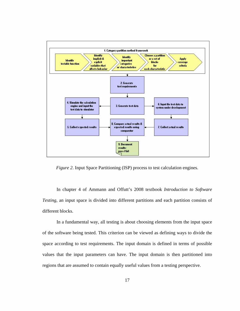
Figure 2. Input Space Partitioning (ISP) process to test calculation engines.
In chapter 4 of Ammann and Offutt’s 2008 textbook Introduction to Software
Testing, an input space is divided into different partitions and each partition consists of
different blocks.
In a fundamental way, all testing is about choosing elements from the input space
of the software being tested. This criterion can be viewed as defining ways to divide the
space according to test requirements. The input domain is defined in terms of possible
values that the input parameters can have. The input domain is then partitioned into
regions that are assumed to contain equally useful values from a testing perspective.
17

Consider a partition q over some domain D. The partition q defines the set of equivalence
classes, which are called blocks that are pairwise disjoint, that is: Bq
Bqbjbijibjbi ∈≠∅=∩ ,;,
and together the blocks cover the domain D, that is:
UBqb
Db∈
=
3.1.1.1 The Category Partition Method
The category partition method provides a process framework in which to partition
the input space. It consists of 6 manual steps to identify input space partitions and convert
them to test cases.
1. Identify functionalities that are called testable functions and can be tested
separately.
2. For each testable function, identify the explicit and implicit variables that can
affect its behavior.
3. For each testable function, identify characteristics or categories that, in the
judgment of the test engineer, are important factors to consider in testing the
function. This is the most creative step in this method and also varies
depending on the expertise of the test engineer.
4. Choose a partition, or set of blocks, for each characteristic. Each block
represents a set of values on which the test engineer expects the software to
behave identically. Well-designed characteristics often lead to straightforward
partitions.
18
5. Choose a test criterion and generate the test requirements. Each partition
contributes exactly one block to a given test requirement.
6. Refine each test requirement into a test case by choosing appropriate values
for the explicit and implicit variables.
3.1.1.2 Coverage Criterion for Input Space Partitioning
Amman and Offutt (2008) discussed the All Combinations, Each Choice, Pair-
Wise, t-Wise, Base Choice, and Multiple Base Choices coverage criteria for the input
space partitioning. Pair-Wise, Base Choice, and Multiple Base Choices coverage criteria
were used to derive the test cases for this thesis’s case studies.
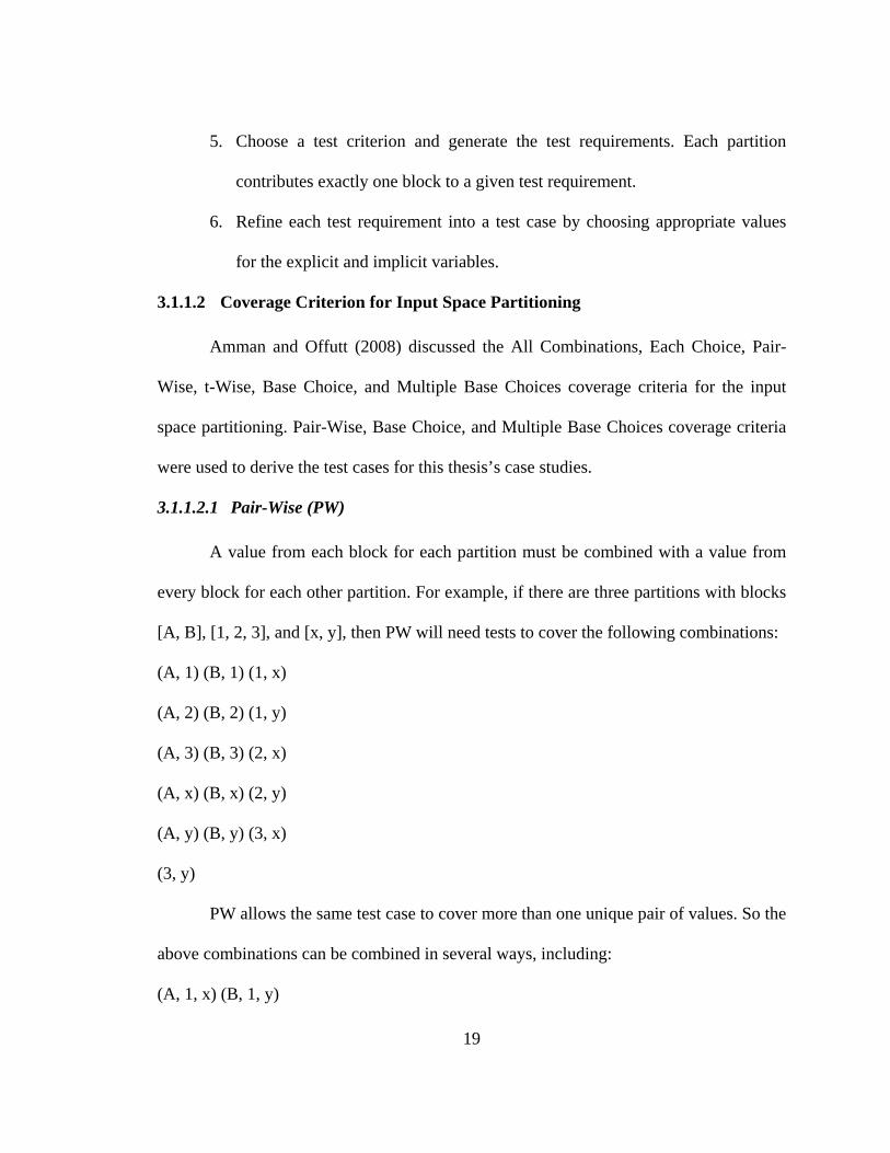
3.1.1.2.1 Pair-Wise (PW)
A value from each block for each partition must be combined with a value from
every block for each other partition. For example, if there are three partitions with blocks
[A, B], [1, 2, 3], and [x, y], then PW will need tests to cover the following combinations:
(A, 1) (B, 1) (1, x)
(A, 2) (B, 2) (1, y)
(A, 3) (B, 3) (2, x)
(A, x) (B, x) (2, y)
(A, y) (B, y) (3, x)
(3, y)
PW allows the same test case to cover more than one unique pair of values. So the
above combinations can be combined in several ways, including:
(A, 1, x) (B, 1, y)
19

(A, 2, x) (B, 2, y)
(A, 3, x) (B, 3, y)
(A, ~, y) (B, ~, x)
The tests with “~” mean that any block can be used. A test suite that satisfies PW will
pair each value with each other value.
3.1.1.2.2 Base Choice (BC)
A base choice block is chosen for each partition, and a base test is formed by
using the base choice for each partition. Subsequent tests are chosen by holding all but
one base choice constant and using each non-base choice in each other parameter.
We actually use domain knowledge to choose the base blocks. The base choice
criterion depends on a crucial piece of domain knowledge: Which block from each
partition determines the base choice test. This choice is called the “base choice.”
If there are three partitions with blocks [A, B], [1, 2, 3], and [x, y], suppose base choice
blocks are ‘A’, ‘1’ and ‘x.’ Then the base choice test is (A, 1, x), and the following tests
would need to be used:
(B, 1, x)
(A, 2, x)
(A, 3, x)
(A, 1, y)
A test suite that satisfies BC will have one base test, plus one test for each remaining
block for each partition.
20
The base choice can be the simplest, the smallest, the first in some ordering, or the
most likely from an end-user point of view. Combining more than one invalid value is
usually not useful because the software often recognizes one value and then negative
effects of the others are masked. Which blocks are chosen for the base choices becomes a
crucial step in test design that can greatly impact the resulting test. It is important to
document the strategy that was used so that further testing can reevaluate that decision.
3.1.1.2.3 Multiple Base Choices (MBC)
At least one, and possibly more, base choice blocks are chosen for each partition,
and base tests are formed by using each base choice for each partition at least once.
Subsequent tests are chosen by holding all but one base choice constant for each base test
and using each non-base choice in each other parameter.
The MBC criterion sometimes results in duplicate tests, which should, of course,
be eliminated.
3.1.2 Requirements Modeling
Modeling the behavior of the software to analyze and derive the tests is known
and has been used for the past four decades. Beizer (1990), Myers, and many others
extensively discussed behavioral testing with the help of models such as control-flow
graphs, transaction-flow graphs, data flow graphs, and finite state machines.
Engineering disciplines use models to develop the products they intend to build.
Requirements models are used to discover and clarify the functional and data
requirements for software and business systems. Additionally, requirements models are
used as specifications for the system’s designers, builders, and testers.
21

Beizer (1990) states that analysis is the engineering process by which a design
evolves to fulfill the requirements. It may be wholly intuitive or formal. Intuitive
analysis, while often effective, cannot be communicated to others easily and,
consequently, some kind of formal, often mathematical, analysis is needed—even if only
retroactively.
Pressman (2005) states that one important step in black box or behavioral testing
is to understand the objects that are modeled in the software and the relationships that
connect those objects. Once this has been accomplished, the next step is to define a series
of tests that verify the statement “All objects have the expected relationship to one
another.” Stated in another way, software testing begins by creating a graph of important
objects and their relationships and then devising a series of tests that will cover the graph
so that each object and relationship is exercised and errors are uncovered.
The idea of modeling different aspects of the system using different modeling
tools is gaining momentum at present. It is also very conventional that test engineers
build mental models as a part of the problem analysis. These models can further be used
to derive the test conditions. Therefore, one objective of modeling the requirements is to
generate the test requirements and then refine the test requirements into test cases by
choosing appropriate values for both the explicit and implicit variables.
Binder (2000) states that software testing requires the use of a model to guide the
efforts in test selection and test verification. Often, such models are implicit, existing
only in the head of a human tester, applying test inputs in an ad hoc fashion. The mental
models testers build encapsulate application behavior, allowing testers to understand the
22

application’s capabilities and more effectively test its range of possible behaviors. When
these models are written down, they become sharable, reusable testing artifacts.
Simply put, a model of software describes behavior. Behavior can be described in
terms of input sequences accepted by the system, the actions, conditions, and output
logic, or the flow of data through the application’s modules and routines. In order for a
model to be useful for groups of testers and for multiple testing tasks, it needs to be taken
out of the mind of those who understand what the software is supposed to accomplish and
written down in an easily understandable form. It is also generally preferable that a model
be as formal as it is practical. With these properties, the model becomes a shareable,
reusable, precise description of the system under test.
There are many such models, and each describes different aspects of software
behavior. For example, control-flow, data-flow, and program dependency graphs express
how the implementation behaves by representing its source code structure. Decision
tables, transaction-flows, and state machines, on the other hand, are used to describe
external so-called black box behavior. The system testing community today tends to think
in terms of such black box models. Finite state machines, state charts, UML models,
grammars, decision tables, and decision trees are some of the popular models used to
represent the software behavior.
In general, test models are designed as part of problem analysis.
The criterion for model testability is an algorithm that can be devised and
programmed that will produce ready-to-run test cases with only the information in the
23

model. The model should support both manual and auto test generation. Binder (2000)
describes that a testable model must meet the following requirements:
The model should be a complete and accurate reflection of the kind of
implementation to be tested. The model must represent all features to be
exercised.
The model should abstract the details that would make the cost of testing
prohibitive.
The model should preserve the details that are essential for revealing faults
and demonstrating conformance.
The model should represent all possible events so that we can generate these
events, typically as messages sent to the system under test.
The model should represent all possible actions so that we can determine
whether a required action has been produced.
The model should represent the state so that we have an executable means to
determine what state has been achieved.
Models also reveal controllability and observability by tracing different paths that
information can flow through in the system. In addition, models provide the visual
representations of the information flow, thus allowing the requirements engineers,
development engineers, and test engineers to have the same understanding of the
requirements.
When multiple projects related to the calculation engines in financial services are
studied, requirements specifications follow a certain pattern when modeled in the form of
24

a graph; if appropriate graph coverage criterion is applied, paths in a graph produce
different test requirements.
There are several techniques available to model the requirements and then to
generate the test requirements from the models. I developed the tool called the Fusion
Test Modeler (FTM) to facilitate modeling the requirements related to calculation
engines. This tool helped test analysts in requirements modeling and then in tracing back
the test cases to the requirements.
The requirements of the calculation engines are captured in the form of sequences
of events, sequences of actions, business rules, use cases, plain text in English, logical
expressions, and mathematical expressions. For example, pricing a loan or a contract
occurs when some events occur, such as creation of the loan, change in time period,
change in the interest rates, and/or change in fee rates. Amortization calculations depend
on the time period of the loan and characteristics of the loan such as ARM or fixed. Asset
valuation triggers a different set of calculations based on the Asset type, e.g. whole loans,
swaps, or bonds.
In some cases, specifications for the calculations are defined in the form of
pseudo-code and procedural design, especially for financial models, which are bought as
third-party tools and are integrated into the Freddie Mac systems. In other cases, complex
calculations are embedded in the sequence of steps in use cases mentioning when to
trigger the calculations.
The modeling design chosen in this thesis is a Tree. Requirements can be
analyzed in the form of models. These models can be further extended and then could be
25

decomposed to trace different paths in the models. These decomposed paths simplify the
complex or obscure behavior of the calculation engines. Each path in the models can be
refined to a unique test case mapping to the test requirement.
Graph in 1G Figure 3 is an example of Tree.
Figure 3. Tree example.
In general, for any graph-based coverage criterion, the idea is to identify the test
requirements in terms of various structures in the graph.
A typical test requirement is met by visiting a particular node or edge or by
touring a particular path. T = {a, b, d}, {a, b, e}, {a, c, f}, {a, c, g} are the four test
requirements that cover the graph in 1G Figure 3.
3.1.3 Overview of the Process
Figure 4 shows the high level process to test the calculation engines using the
modeling technique. The first and second steps are crucial in this process to model the
26

requirements. The Fusion Test Modeler facilitates in modeling the requirements. The
second step in this process is to derive the test scenarios from the model. FTM
automatically generates these test scenarios. Steps 4, 5, and 8 are automated with the help
of other tools.
Figure 4. Modeling process to test calculation engines.
3.1.4 Modeling Technique
The technique defined here is the definitive procedure to be followed in modeling
the requirements to accomplish the goal of deriving the test requirements. These steps
27

follow Beizer’s (1990) advice of modeling and are extended to help modeling using
FTM.
1. Identify the testable functions. This is a manual step; guidelines will be
provided to define the testable function.
2. Examine the requirements and analyze them for operationally satisfactory
completeness and self-consistency.
3. Confirm that the specification correctly reflects the requirements, and correct
the specification if it does not.
4. Rewrite the specification as a sequence of short sentences. This can be done
using FTM.
5. Model the specifications using FTM. Modeling is explained in the subsections
with the examples.
6. Verify the model.
7. Select the test paths. This step is automated.
8. Sensitize the selected test paths. That is, select input values that would cause
the software to do the equivalent of traversing the selected paths.
9. Record the expected outcome for each test. Expected results can be specified
in FTM, which is one of the advantages of the tool.
10. Confirm the path. This step is automated. The prime path coverage criterion
is applied to traverse the model’s paths.
28

3.1.5 Requirements and Specifications
Calculation engines are specified in a variety of formats. Requirements are
translated into functional specifications, which are more formal. In the case of calculation
engines, specifications can take the form of finite state machines, state-transition
diagrams, control flows, process models, data flows, etc. Financial models are sometimes
in the form of the source code; if systems are to be implemented to replicate the financial
models, then the source code becomes the specifications to test. For example, algorithms
defined in the VB language for financial models are to be tested for their implementation
in Java. They are also expressed in combination of all the above, such as logical
expression, use cases, program structures, sequence of events, and sequence of actions.
3.1.5.1 Logical Expressions
Logical expressions generally consist of predicates and clauses. Predicates require
special attention. Compound predicates can be broken down to equivalent sequences of
simple predicates or to disjunctive normal form. Logical expressions can be modeled in
the form of directed acyclic graphs. Clause coverage and predicate coverage criteria can
be used to test the logical expressions. If there are n clauses in the predicate, then
combinatorial coverage leads to truth-values. Applying appropriate predicate and
clause coverage criteria would result in
n2
1+n truth-values. Ammann and Offutt discussed
specification-based logic coverage with examples in chapter 3 of their book (2008).
Predicates in the programs can be taken from if statements, case/switch
statements, for loops, while loops, and do-until loops.
Logical expression can be modeled with the help of the tree shown in Figure 5.
29

Figure 5. Modeling example #1 using Fusion Test Modeler.
3.1.5.2 Use Cases
UML use cases are being widely used to clarify and express software
requirements. They are meant to describe sequences of actions that software performs as
a result of inputs from the users; that is, they help express the workflow of a computer
application. Because use cases are developed early in software development, they can be
valuable in helping the tester start testing activities early.
Use cases are described textually, and can be expressed as graphs. These graphs
can be viewed as transaction flows. Activity diagrams can also be used to express
transaction flows. FTM can be used to model a variety of things, including state changes,
returning values, and computations.
30

For use cases, complete path coverage is often feasible and sometimes reasonable.
It is also rare to find a complicated predicate that contains multiple clauses. This is
because the use case is usually expressed in terms that the users can understand.
Users try to deduce use case scenarios which are instances of, or complete paths
through, a use case. Each scenario should constitute some transaction by the users and is
often derived when the use cases are constructed. If the use case graph is finite, then it is
possible to list all possible scenarios. However, domain knowledge can be used to reduce
the number of scenarios that are useful or interesting from either a modeling or test case
perspective.
3.1.5.3 Loops
The loops themselves are not important for the purpose of modeling, but loop
control variables are important in the cases of both deterministic and non-deterministic
loops. This thesis applied boundary value techniques for the loop control variables.
Deriving these values will help in path sensitization of the processing to be tested within
the loops. This also applies to nested loops.
3.1.5.4 Other Common Elements in Specifications
Various program structures that are commonly seen in the specifications are if-
else structures, nested-if structures, decision tree structures, and case/switch structures.
Conditional expressions are composed of expressions combined with relational and/or
logical operators. A condition is an expression that can be evaluated to be true or false. A
sequence of events, also called preconditions to satisfy, as well as a sequence of actions,
31

relations or constraints defined among different parameters, are some common
observations in the specifications.
All of these structures can be modeled with the help of a tree, as shown in Figure
6.
Figure 6. Modeling example #2 using Fusion Test Modeler.
Requirements modeled as shown in Figures 5 and 6 are transformed into tests as
shown in Figure 7. This process is explained and documented in detail with help of a case
study in Chapters 6 and 9.
32

Figure 7. Sample outputs from Fusion Test Modeler.
3.1.6 Rationale Behind This Modeling Design
The test approach defined here is more appropriate to system testing and
acceptance testing, but can also be applied to unit testing. There are numerous testing
techniques available for black box testing that are insufficient to test calculation engines.
Because controllability and observability are very low for calculation engines,
reachability of a statement or condition can be achieved with the help of modeling.
At present, many commercially available tools expect testers to possess strong
logical, analytical, and critical thinking skills. Unfortunately, this is not always true.
Technology should adequately address the competence of a majority of its users. A
33

number of modeling techniques and tools are also available on the market that take a
longer time to learn and apply, which is not practical. Also, these modeling techniques
are associated with notations and steps to follow. There is a lot of research in generating
test requirements from formal specifications; however, the outcome depends on the
degree of formalism in the specifications.
The trees, on the other hand, are simple structures that can be easily understood
and modeling can be done with ease. FTM is developed to meet the following seven
essential needs.
3.1.6.1 Requirements Traceability
The model’s traceability to the requirements is an essential element that not only
provides the coverage but also helps in impact analysis when requirements change.
Factory tools/modeling languages such as Visio and UML do not help build traceability
into the model. FTM provides traceability of the requirements from the test models.
3.1.6.2 Audit Requirements
Internal audits require testing processes to be transparent. Test cases should be
well documented, and changes should be applied in a controlled manner. FTM allows test
analysts to keep track of changes, and also captures information related to who executed
the tests and when they were executed. Models are saved in XML format and the XML
files can be put under configuration management.
3.1.6.3 Specification Formats
As discussed in Section 2.3, requirements are specified in different formats. FTM
allows modeling multiple kinds of specifications (with some exceptions).
34
3.1.6.4 Easy to Learn
The modeling technique chosen is simple so that the business community, testers,
and analysts from non-engineering backgrounds can learn and model the requirements
with minimal training. They can also analyze the requirements with the help of models.
3.1.6.5 Preserving the Models
It is common for testers to build mental models and then destroy the models once
they understand the requirements. The FTM tool allows users to build rough drafts of the
test models and preserve them for future analysis. The tool helps the users evolve their
analysis into a model that captures the testable requirements. In later stages, it supports
the impact analysis. These models also help in transitioning the knowledge when new
team members arrive into the project.
3.1.6.6 Complementing the Existing Tools to Manage Testing
Freddie Mac has a set of tools that complements its software development
methodology. Any homegrown tools should be tightly integrated with the existing tools.
The FTM tool complements the TestManager tool, which is used to manage the test
assets.
3.1.7 Coverage Criterion
Directed graphs form the foundation for many coverage criteria. For example, the
most common graph abstraction for source code maps code is to a control flow graph. It
is important to understand that the graph is not the same as the artifact; indeed, artifacts
typically have several useful, but nonetheless quite different, graph abstractions. The
same abstraction that produces the graph from the artifact also maps test cases for the
35

artifact to paths in the graph. Accordingly, a graph-based coverage criterion evaluates a
test set for an artifact in terms of how the paths corresponding to the test cases “cover”
the artifact’s graph abstraction.
The basic notion of a graph and necessary additional structures is given below.
A graph G formally is:
• a set N of nodes
• a set of initial nodes, where ⊆ N oN oN
• a set of final nodes, where ⊆ N fN fN
• a set E of edges, where E is a subset of N × N
The term “node” or “vertex” is often identified with a statement or a basic block. The
term “edge” or “arc” is often identified with a branch.
Test criteria require inputs that start at one node and end at another. This is only
possible if a path connects those nodes.
Ammann and Offutt (2008) presented different graph coverage criteria for the
structural graphs and data flow graphs. The Node coverage, Edge coverage, Edge-Pair
coverage, Prime Path coverage, Simple Round Trip coverage, Complete Round Trip
coverage, Complete Path coverage, and Specified Path coverage are applicable for the
structural graphs. The All-DU-Paths coverage, All-Uses coverage, and All-Defs coverage
are applicable for the data flow graphs.
The logical expressions, conditional expressions, and control structures such as if
statements, if-else statements, nested if-else statements, switch statements, and use cases
are modeled in the form of trees using the Fusion Test Modeler (FTM). The tree
36

structures do not have loops. Traversing the tree from root to leaf leads to the prime path
coverage criterion. When there are no loops, the prime path coverage criterion is
equivalent to the all-paths coverage. Therefore, in this case, applying prime path
coverage criterion generates all the distinct paths in the model, which in turn are the test
cases.
3.1.7.1 Prime Path Coverage
A path from to is simple if no node appears more than once on the path,
with the exception that the first and last nodes may be identical.
in jn
A path from to is a prime path if it is a simple path and it does not appear as
a proper subpath of any other simple path.
in jn
Prime Path Coverage (PPC): TR contains each prime path in G.
3.2 Step #2: Generating Test Requirements
The test requirements for the calculation engines are generated from the models
that are built using FTM. Prime path coverage is applied to derive the test requirements.
This process of generating test requirements is automated, which means when
requirements are modeled using FTM, test requirements are automatically generated.
This process is explained in detail in this thesis’s case studies.
For ISP, test requirements for the testable functions are derived by applying Base
Choice (BC), Multiple Base Choice (MBC), and Pair-Wise (PW) coverage criteria.
Testable functions are identified and then their partitions and blocks are derived
following the guidelines in the category partition method framework. Guidelines are
provided to list the partitions and blocks in the spreadsheet. Java utilities are written to
37

read and generate the base choice and multiple base choice test requirements from the
spreadsheet. Bach’s PERL program is used to read and generate the pairwise test
requirements from the spreadsheet.
This step is completely automated.
3.3 Step #3: Generating Test Data
In order to execute the test requirements derived from step #2, test data is
required. This test data is refined from the input space partitioning and modeling
technique.
As discussed in earlier sections, calculation engines usually do not receive inputs
directly from the GUI. Calculations will be triggered only after the inputs are validated at
the presentation layer, which means invalid inputs are unlikely to be input to the
calculation engines. In this process, test data will be associated with the test requirements
and prepared test cases will be executable.
When there are constraints among the attributes, then the test requirements may
contain attribute values such as “Less than,” “Greater than,” or something similar. Actual
values to these attributes are provided. This step currently involves manual intervention
and is explained in detail in the case studies.
3.4 Step #4: Simulating Calculation Engine and Inputting the Test Data
A simulator is used to generate the expected results. Simulators can be written in
any programming language the test analyst is comfortable with. Freddie Mac often uses
MS-Excel to write the functions using built-in functions of Excel. VB Macros also can be
used.
38
In End User Computing (EUC) applications, most calculations should already be
in place, built with the help of VB Macros or Excel functions. When new information
system applications are built to replace these EUCs per Sarbanes Oxley (SOX)
requirements, system upgrades, or any other compliance requirements, existing programs
can be used as simulators.
Simulators provide challenges with respect to correctness. It is difficult to judge
whether the output of the simulator or the output of the system-under-testing is correct.
Differences in these two outcomes should be resolved with the knowledge of a
calculation engine specialist or a requirements analyst.
Simulators should be simple in nature compared to the implementation of the
same logic in system-under-testing. Test inputs derived in step #3 should be inputted to
the simulator. Inputs are generated in large numbers; therefore, automated programs can
be developed to read the inputs and input them to the simulator.
Pemmaraju (1998) states that if multiple calculations performed by different
calculators work in combination to produce the final output, it is beneficial to log the
outputs of each calculator. This will help in two ways. One is to understand the data
flows among these calculators. The second is to know the internal states of these values.
In addition, logging helps to debug the problem if the expected and actual results differ.
3.5 Step #5: Collecting Expected Results
Once the test data is derived and is associated with the test requirements, the test
case now becomes ready to execute. When these test cases are executed against the
simulator built in the previous step, the simulator produces the expected results.
39

The automation process helps generate the tests and execute them in a reasonable
amount of time. Since the models are developed early in the life cycle and undergo
frequent changes, expected results tend to change. A mechanism needs to be established
to capture the expected results. In this thesis’s case studies, expected results are captured
in the spreadsheets under different columns for each test requirement and this placeholder
always remains the same.
In EUC applications in Freddie Mac, when systems are already in place these
expected results are already available in the reference spreadsheets. VB Macros in the
spreadsheets contain the same functionality as the system-under-test. This also comes
with a price, as the reference spreadsheet is just a current form of implementation of a
complex application and therefore could be as faulty as the new implementation of the
system-under-test. Nevertheless, the reference spreadsheet proved to be very useful for
automated verification of results, as it was possible to write scripts to read the
spreadsheet and obtain results from it. Moreover, the reference spreadsheet was the only
specification for the backend calculations in one case study.
3.6 Step #6: Input Test Data to the System-Under-Test
Once the test data is generated and is associated with the test requirements, test
cases are ready to execute against the system-under-test. This process of deriving the
inputs using the ISP method, and designing the test requirements from the test model,
may generate a large number of test cases—making them cumbersome and time
consuming to execute manually. Therefore, an automation tool must be considered to
feed the test data of the test cases to the system under development. In Rational
40

TestManager this test data is stored in data pools. A data-driven testing technique is
applied to automatically enter the test data into the system by the tool. Logic validation is
not added to the automation scripts in order to maximize the processing time of the data
entry. Automation scripts are just simulated to enter the data and are scheduled on
different machines to enter data in parallel. When the test data is inputted to the system,
calculation-triggering events are identified and automation scripts are programmed to
trigger the calculations. Events to trigger the calculations are also incorporated into the
script, so that every time the event triggers, the calculation engine is activated and
performs calculations at the business layer, storing the results in the database.
3.7 Step #7: Collecting Actual Results
All the actual results are stored in the database. It is essential for the test analysts
to understand the data model of the system so they can locate the actual results. In
general, the final state of the actual results generated by the calculation engines will be
stored in the database, and the internal states of the results may be logged into the
execution logs for debugging. It may be required to refer to the execution logs for the
internal states and values of the actual results in case of deviation from the expected
results. In one case study, where there are 9 calculators involved and each calculator
receives the inputs from one or more calculators, it was suggested to programmers to
generate the execution logs with the intermediate values of the calculation variables. This
helped in debugging the incorrect expected output. A Java utility was written to search all
the intermediate states of calculation variables for each and every instance of them. The
41

program scanned 10 MB of the execution logs in less than 10 seconds and wrote the
expected intermediate outputs in a tabular format in an Excel spreadsheet.
3.8 Step #8: Comparing Actual and Expected Results Using a Comparator
Because the calculations performed by the backend often produced hundreds of
outputs, an automated comparison tool was developed to examine and compare the
backend results with those of the spreadsheet. Also, these results need to be compared
more frequently. The comparator compares the results, showing the differences in cases
of failures and showing success in cases of passes. Expected results are saved in the
Excel sheet and actual results may be obtained from the database or execution logs. The
comparator is built with the capability to compare the left-hand side and right-hand side
of the results in different forms: spreadsheet, spreadsheet; spreadsheet, database; and
spreadsheet, text file.
In some cases, actual results (intermediate) are obtained from the program
execution logs. These logs store values for intermediate results and final results are stored
in the database. The comparator searches for the desired text in the execution logs and
required fields in the database. The comparator tool discards unneeded text strings before
making comparisons of the output results. Actual and expected results may not always be
the same. As long as they are with in the tolerance limits, the result is deemed correct.
For example, a variation of at most one dollar in a million is acceptable if the variation is
caused due to drifts in floating point accuracy in Java or Microsoft Excel.
42

4 Case Study #1: Contract Pricing
“Contract Pricing” is an important feature in the pricing subsystem of the selling
system. The system prices the contracts when contracts are created in the Loan Purchase
Contract (LPC) subsystem and reprices the contracts when contracts are modified or upon
a request from the user.
The contracts are of two types: cash contracts and swap contracts. This case study
represents swap contract pricing. The requirements for the pricing calculations of swap
contracts are specified in the form of use cases. This use case calculates the swap GFee,
Buyup max, Buydown max, and Total adjusted GFee for fixed rate, Guarantor, and
Multilender ARM swap contracts.
This thesis is focused on the approach to test the calculation engines; however,
this case study also shows how to isolate and test the testable functions related to
calculations in the system. Freddie Mac’s selling system consists of different subsystems:
LPC, NCM, TPA, Pooling, Pricing, and OIM. Each subsystem contains multiple features
and is designed to abstract their functionalities from the other. The “contract pricing”
feature in the pricing subsystem receives the inputs from the “import contracts” feature of
the LPC subsystem that facilitates importing the contracts. This feature is tested in two
stages. In the first stage, the import contracts feature is tested so that the system accepts
43

only the valid contracts for pricing. In the second stage, contract attributes are isolated to
test the contract pricing feature of the system.
4.1 Step #1: Input Space Partitioning
The contract entity has 29 attributes. Therefore, the contract domain is divided
into 29 partitions. These partitions and their blocks are shown in Table 1.
44

Table 1: Contract Partitions and Blocks
Partition Partition Name Partition Blocks
1 Execution Option {GU, ML, NULL_EO, *EO} 2 Rate Option {FI, AR, NULL_RO, *RO} 3 Master Commitment {9CHAR, 10CHAR, 8CHAR,NULL_MC, TBD} 4 Security Product {NUMBER, NULL_SP, *SP} 5 Security Amount {DOLLAR_ROUND, *DOLLAR_FRACTION,
*>100B, NULL_SA} 6 Contract Name {CHAR (26), CHAR (25), CHAR (1),
NULL_CONT} 7 Settlement Date {MMDDYYYY, *SD, NULL_SD} 8 Settlement Cycle Days {1,3,4,5, *6, *2, NULL_SCD} 9 Security Coupon {XX.XXX, XXX.XX, NULL_SC, 26.000} 10 Servicing Option {RE, CT, *SO, NULL_SO} 11 Designated Servicer Number {NULL_DS, DS, *DS} 12 Minimum Required Servicing
Spread {XX.XXX, NULL_MRSS, XXX.XX}
13 Minimum Servicing Spread Coupon
{XX.XXX, NULL_MSSC, XXX.XX}
14 Minimum Servicing Spread Margin
{XX.XXX, NULL_MSSM, XXX.XX}
15 Minimum Servicing Spread Lifetime Ceiling
{XX.XXX, NULL_MSSLC, XXX.XX}
16 Remittance Option {AR, SU, FT, GO, *RT, NULL_RT} 17 Super ARC Remittance Due day {0,1,2,14,15,16,NULL_SARD} 18 Required Spread GFee {NULL_RSG, *RSG, RSG} 19 BUBD Program Type {CL, NL, LL, *BUBD_PT, NULL} 20 BUBD Request Type {NULL_BUBD_RT, BO, BU, BD, NO,
*BUBD_RT} 21 Contract Level Buyup/Buydown {NULL_CL_BUBD, *CL_BUBD, BU, BD, NO} 22 BUBD Grid Type {NULL_BUBD_GT, *BUBD_GT, A, A-Minus,
Negotiated 1 Grid} 23 BU Max Amount {0, *BU_MAX_AMT, NULL_BU_MAX_AMT,
XXX.XXX} 24 BD Max Amount {0, *BD_MAX_AMT, NULL_BD_MAX_AMT,
XXX.XXX} 25 Pool Number {NULL_PNO, PNO, *PNO} 26 Index Look Back Period {NULL_ILP, *ILP, ILP} 27 Fee Type {FT, *FT, NULL_FT} 28 Fee Payment Method {Delivery Fee, GFee Add On, *FTM,
NULL_FTM} 29 Prepayment Penalty Indicator {Y, N}
45

The system validates the properties for each attribute before creating a contract
and generates an error message if any invalid inputs or invalid combination of inputs are
passed to the system.
The blocks for each partition are derived based on the system specifications. The
standard conventions are followed in defining the abstract values for these blocks. For
example, for the first partition, Execution Option, the set of blocks are: {GU, ML,
NULL_EO, *EO}. GU and ML are valid values for this partition. Invalid values are
represented by *EO, which means the user can pass any satisfying value in the place of
*EO. NULL_EO is another invalid value per the specifications. When the values for
*EO, and NULL_EO are inputted, the system is expected to generate error messages
informative to the user. This feature is tested in two stages.
First Stage
In the first stage, each attribute of the contract is validated using the base choice
coverage criterion and constraints among the attributes are validated using the pair-wise
coverage criterion.
The base contract is chosen to create the base choice contracts using different
values of the blocks from each partition. A Java utility was written to create the base
choice contracts.
When each block of every partition needs to be validated, the base choice
coverage works well. Each base choice contract is targeted to validate one of the business
rules in case of valid values, or will be targeted to generate error or informative messages
in case of invalid values.
46
Even though one test input or a base contract addresses more than one
requirement, independent tests are created to satisfy each requirement. This not only
helps in traceability of the requirements, but also helps minimize the changes in test
cases.
In the first stage, all the attributes or partitions of the contract are treated as being
independent even though the constraints exist.
The constraints among the parameters are tested as follows: The Rate option,
BUBD eligibility type, and BUBD request type of the contract are interdependent and
also depend on the values of another entity called a master commitment. The master
commitment has 30 partitions but MC LLBUBD eligibility and MC GFee add on
eligibility are the only partitions within the scope of this testable function.
The pair-wise coverage criterion is applied to derive test cases to test the
constraints among these parameters. Other partitions of the contract are prefixed with the
base test value of the contract.
Each and every distinct value chosen for the blocks are traced to different error
messages and an error code associated with it. Inputs are derived based on the functional
specifications and not from the implementation details. Some tests are infeasible, as the
design does not allow them. It is also a good practice to derive the inputs based on the
functional specifications instead of implementation details, as the tests may uncover the
errors in implementation (Grindal, Offut & Mellin, 2006).
47

Applying the base choice technique produced 120 test cases for contracts; pair-
wise produced 207 test cases. A Java utility was built to generate base choice test cases
and Bach’s Perl program was used to generate the pair-wise test cases.
The contract entity has close to 200 business rules defined for the import contracts
feature in the LPC subsystem. Test inputs are derived in the above process by applying
the base choice and pair-wise coverage criteria to satisfy each and every business rule.
Second Stage
In the second stage, partitions required for “contract pricing” calculations were
separated and then base choice, multiple base choice, and pair-wise criteria are applied.
Problem analysis shows that among the inputs defined earlier, only Rate option, GFee,
Remittance option type, GFee grid remittance option, LLGFee eligibility, BUBD
Eligibility, and Max Buyup determine the controllability of the calculations. Therefore,
only these partitions are considered to derive the tests. Partitions and blocks of the
Contract Pricing are shown in Table 2.
.
Table 2: Contract Pricing Partitions and Blocks
Partitions Rate Option GFee
Remittance Option Type
GFee Grid Remittance
Option
MC LLGFee
Eligibility
BUBD Eligibility
Max Buyup
{LT_12.5,
EQ_12.5,
GT_12.5,
NULL}
Blocks {FIXE
D, ARM}
{NOT_NULL, NULL}
{GOLD, FIRST_TUESDAY,
ARC, SUPER_A
RC}
{GOLD, FIRST_TUE
SDAY, ARC,
SUPER_ARC}
{Y, N}
{PROHIBITED,
REQUIRED,
OPTIONAL}
48

Base test #1, selected to generate base choice tests, is shown in Table 3.
Table 3: Contract Pricing Base Test #1
Partitions Rate Option GFee Remittance
Option Type
GFee Grid Remittance
Option
MC LLGFee
Eligibility
BUBD Eligibility
Max Buyup
Blocks FIXED NOT_NULL GOLD GOLD
PROHIBITED
LT_12.5 Y
Base test #2, selected to generate base choice tests, is shown in Table 4. Table 4: Contract Pricing Base Test #2
Partitions Rate Option GFee
Remittance Option Type
GFee Grid Remittance
Option
MC LLGFee
Eligibility
BUBD Eligibility
Max Buyup
Blocks ARM NOT_NULL
SUPER_ARC
PROHIBITED
EQ_12.5 GOLD N
4.1.1 Base Choice Coverage
Table 5 shows the base choice tests generated using base choice test #1.
49

Table 5: Contract Pricing Base Choice Tests
Test #
Rate Option GFee Remittance
Option Type
GFee Grid Remittance
Option
MC LLGFee
Eligibility
BUBD Eligibility
Max Buyup
1 ARM NOT_NULL GOLD GOLD Y PROHIBITED LT_12.5
2 FIXED NULL GOLD GOLD Y PROHIBITED LT_12.5
3 FIXED NOT_NULL
FIRST_ TUESDAY GOLD Y PROHIBITED LT_12.5
4 FIXED NOT_NULL ARC GOLD Y PROHIBITED LT_12.5
5 FIXED NOT_NULL
SUPER_ARC GOLD Y PROHIBITED LT_12.5
6 FIXED NOT_NULL GOLD
FIRST_TUESDAY Y PROHIBITED LT_12.5
7 FIXED NOT_NULL GOLD ARC Y PROHIBITED LT_12.5
8 FIXED NOT_NULL GOLD
SUPER_ARC Y PROHIBITED LT_12.5
9 FIXED NOT_NULL GOLD GOLD N PROHIBITED LT_12.5
10 FIXED NOT_NULL GOLD GOLD Y REQUIRED LT_12.5
11 FIXED NOT_NULL GOLD GOLD Y OPTIONAL LT_12.5
12 FIXED NOT_NULL GOLD GOLD Y PROHIBITED
EQ_12.5
13 FIXED NOT_NULL GOLD GOLD Y PROHIBITED
GT_12.5
14 FIXED NOT_NULL GOLD GOLD Y PROHIBITED NULL
15 FIXED NOT_NULL GOLD GOLD Y PROHIBITED LT_12.5
4.1.2 Multiple Base Choice Coverage
Table 6 shows the multiple base choice tests using base choice test #1 and base
choice test #2.
50

Table 6: Contract Pricing Multiple Base Choice Tests
Test #
Rate Option GFee
Remittance Option Type
GFee Grid Remittance
Option
MC LLGFee
Eligibility
BUBD Eligibility
Max Buyup
1 ARM NOT_NULL GOLD GOLD Y PROHIBITED LT_12.5
2 FIXED NULL GOLD GOLD Y PROHIBITED LT_12.5
3 FIXED NOT_NULL
FIRST_ TUESDAY GOLD Y PROHIBITED LT_12.5
4 FIXED NOT_NULL ARC GOLD Y PROHIBITED LT_12.5
5 FIXED NOT_NULL
SUPER_ ARC GOLD Y PROHIBITED LT_12.5
6 FIXED NOT_NULL GOLD
FIRST_ TUESDAY Y PROHIBITED LT_12.5
7 FIXED NOT_NULL GOLD ARC Y PROHIBITED LT_12.5
8 FIXED NOT_NULL GOLD
SUPER_ ARC Y PROHIBITED LT_12.5
9 FIXED NOT_NULL GOLD GOLD N PROHIBITED LT_12.5
10 FIXED NOT_NULL GOLD GOLD Y REQUIRED LT_12.5
11 FIXED NOT_NULL GOLD GOLD Y OPTIONAL LT_12.5
12 FIXED NOT_NULL GOLD GOLD Y PROHIBITED EQ_12.5
13 FIXED NOT_NULL GOLD GOLD Y PROHIBITED GT_12.5
14 FIXED NOT_NULL GOLD GOLD Y PROHIBITED NULL
15 FIXED NOT_NULL GOLD GOLD Y PROHIBITED LT_12.5
16 FIXED NOT_NULL
SUPER_ ARC GOLD N PROHIBITED EQ_12.5
17 ARM NULL SUPER_ ARC GOLD N PROHIBITED EQ_12.5
18 ARM NOT_NULL GOLD GOLD N PROHIBITED EQ_12.5
19 ARM NOT_NULL
FIRST_ TUESDAY GOLD N PROHIBITED EQ_12.5
20 ARM NOT_NULL ARC GOLD N PROHIBITED EQ_12.5
21 ARM NOT_NULL
SUPER_ ARC
FIRST_ TUESDAY N PROHIBITED EQ_12.5
22 ARM NOT_NULL
SUPER_ ARC ARC N PROHIBITED EQ_12.5
23 ARM NOT_NULL
SUPER_ ARC
SUPER_ ARC N PROHIBITED EQ_12.5
24 ARM NOT_NULL
SUPER_ ARC GOLD Y PROHIBITED EQ_12.5
25 ARM NOT_NULL
SUPER_ ARC GOLD N REQUIRED EQ_12.5
51

Remittance Option Type
Test #
Rate Option GFee
GFee Grid Remittance
Option
MC LLGFee
Eligibility
BUBD Eligibility
Max Buyup
26 ARM NOT_NULL
SUPER_ ARC GOLD N OPTIONAL EQ_12.5
27 ARM NOT_NULL
SUPER_ ARC GOLD N PROHIBITED LT_12.5
28 ARM NOT_NULL
SUPER_ ARC GOLD N PROHIBITED GT_12.5
29 ARM NOT_NULL
SUPER_ ARC GOLD N PROHIBITED NULL
30 ARM NOT_NULL
SUPER_ ARC GOLD N PROHIBITED EQ_12.5
4.1.3 Pair-Wise Coverage
Table 7 shows the pair-wise tests derived using Bach’s PERL program.
52

Table 7: Contract Pricing Pair-Wise Tests
Test #
Rate Option GFee
Remittance Option Type
GFee Grid Remittance
Option
MC LLGFee
Eligibility
BUBD Eligibility
Max Buyup
1 FIXED NOT_NULL GOLD GOLD Y PROHIBITED LT_12.5
2 ARM NULL FIRST_ TUESDAY GOLD N REQUIRED EQ_12.5
3 FIXED NULL FIRST_ TUESDAY
FIRST_ TUESDAY Y OPTIONAL LT_12.5
4 ARM NOT_NULL GOLD FIRST_ TUESDAY N PROHIBITED EQ_12.5
5 FIXED NOT_NULL ARC ARC N REQUIRED GT_12.5
6 ARM NOT_NULL SUPER_ ARC ARC Y OPTIONAL NULL
7 FIXED NULL SUPER_ ARC SUPER_ARC N PROHIBITED GT_12.5
8 ARM NULL ARC SUPER_ARC Y REQUIRED NULL 9 ARM NULL GOLD ARC N REQUIRED LT_12.5
10 FIXED NOT_NULL FIRST_ TUESDAY SUPER_ARC Y OPTIONAL EQ_12.5
11 ARM ~NULL GOLD GOLD Y OPTIONAL GT_12.5
12 FIXED ~NOT_NULL
FIRST_ TUESDAY
FIRST_ TUESDAY N PROHIBITED NULL
13 ~ARM ~NOT_NULL ARC
FIRST_ TUESDAY N OPTIONAL GT_12.5
14 ~FIXED ~NULL ARC ARC ~Y PROHIBITED EQ_12.5
15 ~FIXED ~NOT_NULL
SUPER_ ARC GOLD ~N REQUIRED NULL
16 ~ARM ~NOT_NULL
SUPER_ ARC SUPER_ARC ~N ~PROHIBITED LT_12.5
17 ~FIXED ~NULL SUPER_ ARC
FIRST_ TUESDAY ~Y REQUIRED GT_12.5
18 ~FIXED ~NULL GOLD GOLD ~N ~OPTIONAL NULL
19 ~ARM ~NOT_NULL ARC GOLD ~Y ~PROHIBITED LT_12.5
20 ~ARM ~NOT_NULL
FIRST_ TUESDAY ARC ~Y ~REQUIRED EQ_12.5
21 ~FIXED ~NULL GOLD SUPER_ARC ~N ~OPTIONAL EQ_12.5
22 ~ARM ~NULL FIRST_ TUESDAY
~FIRST_ TUESDAY ~Y ~PROHIBITED GT_12.5
23 ~ARM ~NULL SUPER_ ARC ~ARC ~N ~OPTIONAL EQ_12.5
4.2 Step # 1: Modeling Technique
The testable function for the Contract Pricing is modeled using the FTM tool.
Detailed outputs of the model are shown in Appendix A. Test cases are shown in Table 8.
53

Table 8: Contract Pricing Test Inputs From Modeling
Test #
Rate Option GFee
Remittance Option Type
GFee Grid Remittance
Option
MC LLGFee
Eligibility
BUBD Eligibility
Max Buyup
1 FIXED NOT_NULL GOLD GOLD Y PROHIBITED GT_12.5 2 FIXED NOT_NULL GOLD GOLD Y PROHIBITED LE_12.5 3 FIXED NOT_NULL GOLD GOLD Y PROHIBITED GT_12.5 4 FIXED NOT_NULL GOLD GOLD Y PROHIBITED LE_12.5
5 FIXED NOT_NULL GOLD SUPER_ ARC Y PROHIBITED GT_12.5
6 FIXED NOT_NULL GOLD SUPER_ ARC Y PROHIBITED GT_12.5
7 FIXED NOT_NULL GOLD FIRST_ TUESDAY Y PROHIBITED LE_12.5
8 FIXED NOT_NULL GOLD ARC Y PROHIBITED LE_12.5
9 FIXED NOT_NULL GOLD FIRST_ TUESDAY Y PROHIBITED LE_12.5
10 FIXED NOT_NULL GOLD FIRST_ TUESDAY Y PROHIBITED GT_12.5
11 FIXED NOT_NULL GOLD ARC Y PROHIBITED LE_12.5
12 FIXED NOT_NULL GOLD FIRST_ TUESDAY Y PROHIBITED LE_12.5
13 FIXED NOT_NULL GOLD GOLD N PROHIBITED GT_12.5 14 FIXED NOT_NULL GOLD GOLD N PROHIBITED LE_12.5
15 FIXED NOT_NULL GOLD SUPER_ ARC N PROHIBITED GT_12.5
16 FIXED NOT_NULL GOLD SUPER_ ARC N PROHIBITED LE_12.5
17 FIXED NOT_NULL GOLD SUPER_ ARC N PROHIBITED GT_12.5
18 FIXED NOT_NULL GOLD SUPER_ ARC N PROHIBITED LE_12.5
19 ARM NOT_NULL FIRST_ TUESDAY
FIRST_ TUESDAY Y PROHIBITED GT_25
20 ARM NOT_NULL FIRST_ TUESDAY
FIRST_ TUESDAY Y PROHIBITED LE_25
21 ARM NOT_NULL FIRST_ TUESDAY ARC Y PROHIBITED GT_25
22 ARM NOT_NULL FIRST_ TUESDAY ARC Y PROHIBITED LE_25
23 ARM NOT_NULL FIRST_ TUESDAY
SUPER_ ARC Y PROHIBITED GT_25
24 ARM NOT_NULL FIRST_ TUESDAY
SUPER_ ARC Y PROHIBITED LE_25
25 ARM NOT_NULL FIRST_ TUESDAY
FIRST_ TUESDAY N PROHIBITED GT_12.5
26 ARM NOT_NULL FIRST_ TUESDAY ARC N PROHIBITED EQ_12.5
27 ARM NOT_NULL FIRST_ TUESDAY ARC N PROHIBITED EQ_12.5
54

4.3 Step #2: Generating Test Requirements
Sections 4.1 and 4.2 shows the test cases generated by both the ISP and modeling
technique for the contract pricing feature. The remaining attributes of the contract are
prefixed to make these test cases executable.
4.4 Step #3: Generating Test Data
Test data is built by passing actual values in place of abstract values such as
EQ_12.5, LE_25.
4.5 Step #4: Building the Simulator and Inputting Test Data
The contract pricing calculation simulator was built in Java. This simulator
program reads inputs from the spreadsheet, performs the calculations, and then outputs
the calculation results into another spreadsheet at a defined location. Test inputs derived
from the modeling and ISP techniques are then inputted to the calculation simulator. The
calculation simulator performs the calculations and generates the expected results for
each and every test input. The simulator program also writes the expected results into a
spreadsheet.
4.6 Step #5: Input Test Data Into System-Under-Test
Test inputs derived from the modeling and ISP techniques are then inputted to the
system-under-test. Because we have too many tests to enter them manually, a data-driven
automation technique is applied using the Rational’s robot tool. The system has another
feature called “import contracts” with which all these test inputs can be bundled into a
flat file and imported at once. Both methods are chosen to input the contracts into the
system-under-test, as they follow different paths of processing. When the contract is
55

successfully created, the system automatically prices the contracts and stores the pricing
results in the database. These pricing results are the actual results.
4.7 Steps # 6, 7, and 8: Collecting Expected Results, Actual Results, and
Comparing the Results
Expected results are stored in a spreadsheet and actual results are stored in a DB2
database. The comparator program written in Java compares the expected results with
actual results. The program uses the contract number as the unique ID; it parses the
expected results in the spreadsheet row by row, picks up each contract ID and values of
its attributes, then searches the corresponding values of attributes for the same contract
ID in the database, and compares both the values. If the values match, the program flags
the test case as “Pass,” otherwise as “Fail.” In the calculations, tolerance will be defined
for rounding and is taken into account if the expected and actual results deviate within the
determined tolerance range.
Results and observations are discussed in Chapter 8.
56

5 Case Study #2: Loan Pricing
The “Loan Pricing” feature in the pricing subsystem prices the loans when the
loans are newly created in the system or upon a reprice request by the business users.
In release 7.0, price recalculation for swap loans is triggered by a data correction
to one or more data elements that are used in the price calculation performed at the time
of settlement. These data corrections can be one or both of the following changes:
internal FM price definition terms (grid data), or seller delivered loan/contract data for
price affecting fields. Either type of data correction will trigger a total price recalculation
of all price components that apply to the loan, including GFEE/LLGFEE, BUBD and
Delivery Fees.
The Price recalculation can be approved either automatically or manually. Manual
approval of the price recalculation results is applicable only when the recalculation is
isolated solely to changes in either the BUBD and contract GFEE fee grid definition
changes.
Any data change to loan and/or delivery fee data will trigger a recalculation and
reprice all price component data that is effective at the time of settlement. This includes
any changes to BUBD or contract GFEE grid definition terms.
The mortgage loan entity has nearly 150 attributes, but only a few of those
attributes are relevant to “Loan Pricing” as described in the requirements. Following are
57

12 partitions that are identified in this testable function and shown in Table 9. Among the
12, values for loan interest rate (3), and servicing fee rate (4) are received from the price
grids. These values are updated in the grids based on the current market. Max BU (9),
Max BD (11), and user requested Max Buy Up (12) are intermediate parameters whose
values are used in the final calculations. Even though they participate in the calculations,
their values depend on the values of the other attributes that are input for the loan.
Table 9: Loan Pricing Partitions and Blocks
Partition # Partition Name Partition Blocks
1 BUBD Request Type { NLBUBD, LLBUBD, CLBU, CLBD, NONE } 2 Current Loan Family Type { ARM, FIXED, BALLOON } 3 Loan Interest Rate 4 Servicing Fee Rate 5 Total Adjusted GFee { GT_MAXBD, LT_MAXBD, EQ_MAXBD } 6 BUBD Basis Points { GT_Z, LT_Z, EQ_Z, GT_SSBU, LT_SSBU,
EQ_SSBU, GT_URMP, LT_URMP, EQ_URMP, GT_MAXBD, LT_MAXBD, EQ_MAXBD }
7 Investor Pass Thru Rate 8 Seller Specified Buy Up (SSBU) { GT_MAXBU, LT_MAXBU, EQ_MAXBU } 9 MAX BU 10 Seller Specified Buy Down
(SSBD) { GT_TGF, LT_TGF, EQ_TGF, GT_BUBDBP, LT_BUBDBP, EQ_BUBDBP,
11 MAX BD 12 User Requested Max Buy Up
Among the 140 attributes of the loan, only the 12 partitions shown in Table 9 are
involved in the pricing calculations. Among these 12 partitions, only 6 partitions (1, 2, 5,
6, 8, and 10) influence the controllability of the pricing calculations. The remaining 6
partitions influence the observability of the calculations.
58

5.1 Step #1: Input Space Partitioning
Test cases are derived based on the base choice, multiple-base choice, and pair-
wise coverage criteria taking the partitions that influence the controllability of the loan
pricing calculations. Values for the remaining partitions are prefixed with default values.
The base tests shown in Tables 10 and 11 are used to generate base choice tests and
multiple base choice tests with the help of a Java utility.
Table 10: Loan Pricing Base Test #1
BUBD Request
Type
Loan Type
Total Adjusted
GFee
BUBD Basis points
Seller Specified Buy Up
Seller Specified Buy Down
NLBUBD FIXED GT_MAXBD
GT_MAXBU GT_Z GT_TGF
Table 11: Loan Pricing Base Test #2
BUBD Request
Type
Loan Type
Total Adjusted
GFee
BUBD Basis points
Seller Specified Buy Up
Seller Specified Buy Down
NLBUBD FIXED GT_MAXBD GT_Z
GT_MAXBU GT_TGF
59

5.1.1 Base Choice Coverage
Table 12 shows the base choice tests using base test #1.
Table 12: Loan Pricing Base Choice Tests
Test # BUBD
Request Type
Loan Type
Total Adjusted
GFee
BUBD Basis Points
Seller Specified Buy Up
Seller Specified Buy
Down
1 NLBUBD FIXED GT_MAXBD GT_Z
GT_MAXBU GT_TGF
2 CLBU FIXED GT_MAXBD GT_Z
GT_MAXBU GT_TGF
3 CLBD FIXED GT_MAXBD GT_Z
GT_MAXBU GT_TGF
4 NONE FIXED GT_MAXBD GT_Z
GT_MAXBU GT_TGF
5 LLBUBD ARM GT_MAXBD GT_Z
GT_MAXBU GT_TGF
6 LLBUBD FIXED LT_MAXBD GT_Z
GT_MAXBU GT_TGF
7 LLBUBD FIXED EQ_MAXBD GT_Z
GT_MAXBU GT_TGF
8 LLBUBD FIXED GT_MAXBD EQ_Z
GT_MAXBU GT_TGF
9 LLBUBD FIXED GT_MAXBD LT_Z
GT_MAXBU GT_TGF
10 LLBUBD FIXED GT_MAXBD GT_SSBU
GT_MAXBU GT_TGF
11 LLBUBD FIXED GT_MAXBD LT_SSBU
GT_MAXBU GT_TGF
12 LLBUBD FIXED GT_MAXBD EQ_SSBU
GT_MAXBU GT_TGF
13 LLBUBD FIXED GT_MAXBD GT_URMP
GT_MAXBU GT_TGF
14 LLBUBD FIXED GT_MAXBD LT_URMP
GT_MAXBU GT_TGF
15 LLBUBD FIXED GT_MAXBD EQ_URMP
GT_MAXBU GT_TGF
16 LLBUBD FIXED GT_MAXBD
GT_MAXBD
GT_MAXBU GT_TGF
17 LLBUBD FIXED GT_MAXBD
LT_MAXBD
GT_MAXBU GT_TGF
18 LLBUBD FIXED GT_MAXBD
EQ_MAXBD
GT_MAXBU GT_TGF
60

Test # BUBD
Request Type
Loan Type
Total Adjusted
GFee
BUBD Basis Points
Seller Specified Buy Up
Seller Specified Buy
Down
19 LLBUBD FIXED GT_MAXBD GT_Z
LT_MAXBU GT_TGF
20 LLBUBD FIXED GT_MAXBD GT_Z
EQ_MAXBU GT_TGF
21 LLBUBD FIXED GT_MAXBD GT_Z
GT_MAXBU LT_TGF
22 LLBUBD FIXED GT_MAXBD GT_Z
GT_MAXBU EQ_TGF
23 LLBUBD FIXED GT_MAXBD GT_Z
GT_MAXBU GT_BUBDBP
24 LLBUBD FIXED GT_MAXBD GT_Z
GT_MAXBU LT_BUBDBP
25 LLBUBD FIXED GT_MAXBD GT_Z
GT_MAXBU EQ_BUBDBP
26 LLBUBD GT_MAXBD
GT_MAXBU GT_TGF FIXED GT_Z
5.1.2 Multiple Base Choice Coverage
The test cases in Table 13 are generated using multiple base choice coverage
criteria.
61

Table 13: Loan Pricing Multiple Base Choice Tests
Test # BUBD
Request Type
Loan Type
Total Adjusted
GFee
BUBD Basis Points
Seller Specified Buy Up
Seller Specified Buy
Down
1 NLBUBD FIXED GT_MAXBD GT_Z
GT_MAXBU GT_TGF
2 CLBU FIXED GT_MAXBD GT_Z
GT_MAXBU GT_TGF
3 CLBD FIXED GT_MAXBD GT_Z
GT_MAXBU GT_TGF
4 NONE FIXED GT_MAXBD GT_Z
GT_MAXBU GT_TGF
5 LLBUBD ARM GT_MAXBD GT_Z
GT_MAXBU GT_TGF
6 LLBUBD FIXED LT_MAXBD GT_Z
GT_MAXBU GT_TGF
7 LLBUBD FIXED EQ_MAXBD GT_Z
GT_MAXBU GT_TGF
8 LLBUBD FIXED GT_MAXBD EQ_Z
GT_MAXBU GT_TGF
9 LLBUBD FIXED GT_MAXBD LT_Z
GT_MAXBU GT_TGF
10 LLBUBD FIXED GT_MAXBD GT_SSBU
GT_MAXBU GT_TGF
11 LLBUBD FIXED GT_MAXBD LT_SSBU
GT_MAXBU GT_TGF
12 LLBUBD FIXED GT_MAXBD EQ_SSBU
GT_MAXBU GT_TGF
13 LLBUBD FIXED GT_MAXBD GT_URMP
GT_MAXBU GT_TGF
14 LLBUBD FIXED GT_MAXBD LT_URMP
GT_MAXBU GT_TGF
15 LLBUBD FIXED GT_MAXBD EQ_URMP
GT_MAXBU GT_TGF
16 LLBUBD FIXED GT_MAXBD
GT_MAXBD
GT_MAXBU GT_TGF
17 LLBUBD FIXED GT_MAXBD
LT_MAXBD
GT_MAXBU GT_TGF
18 LLBUBD FIXED GT_MAXBD
EQ_MAXBD
GT_MAXBU GT_TGF
19 LLBUBD FIXED GT_MAXBD GT_Z
LT_MAXBU GT_TGF
20 LLBUBD FIXED GT_MAXBD GT_Z
EQ_MAXBU GT_TGF
21 LLBUBD FIXED GT_MAXBD GT_Z
GT_MAXBU LT_TGF
62

BUBD Request
Type
Total Adjusted
GFee
Seller Specified Buy Up
Seller Specified Buy
Down
Loan Type
BUBD Basis Points Test #
GT_MAXBD
GT_MAXBU 22 LLBUBD FIXED GT_Z EQ_TGF
GT_MAXBD
GT_MAXBU 23 LLBUBD FIXED GT_Z GT_BUBDBP
GT_MAXBD
GT_MAXBU 24 LLBUBD FIXED GT_Z LT_BUBDBP
GT_MAXBD
GT_MAXBU 25 LLBUBD FIXED GT_Z EQ_BUBDBP
GT_MAXBD
GT_MAXBU 26 LLBUBD FIXED GT_Z GT_TGF
GT_MAXBD
GT_MAXBU 27 LLBUBD ARM GT_Z GT_TGF
GT_MAXBD
GT_MAXBU 28 CLBU ARM GT_Z GT_TGF
GT_MAXBD
GT_MAXBU 29 CLBD ARM GT_Z GT_TGF
GT_MAXBD
GT_MAXBU 30 NONE ARM GT_Z GT_TGF
GT_MAXBD
GT_MAXBU 31 NLBUBD FIXED GT_Z GT_TGF
LT_MAXBD
GT_MAXBU 32 NLBUBD ARM GT_Z GT_TGF
EQ_MAXBD
GT_MAXBU 33 NLBUBD ARM GT_Z GT_TGF
GT_MAXBD
GT_MAXBU 34 NLBUBD ARM EQ_Z GT_TGF
GT_MAXBD
GT_MAXBU 35 NLBUBD ARM LT_Z GT_TGF
GT_MAXBD
GT_MAXBU 36 NLBUBD ARM GT_SSBU GT_TGF
GT_MAXBD
GT_MAXBU 37 NLBUBD ARM LT_SSBU GT_TGF
GT_MAXBD
GT_MAXBU 38 NLBUBD ARM EQ_SSBU GT_TGF
GT_MAXBD
GT_MAXBU 39 NLBUBD ARM GT_URMP GT_TGF
GT_MAXBD 40 NLBUBD ARM LT_URMP
GT_MAXBU GT_TGF
41 NLBUBD ARM GT_MAXBD EQ_URMP
GT_MAXBU GT_TGF
42 NLBUBD ARM GT_MAXBD
GT_MAXBD
GT_MAXBU GT_TGF
43 NLBUBD ARM GT_MAXBD
LT_MAXBD
GT_MAXBU GT_TGF
44 NLBUBD ARM GT_MAXBD
EQ_MAXBD
GT_MAXBU GT_TGF
45 NLBUBD ARM GT_MAXBD GT_Z
LT_MAXBU GT_TGF
63

Test # BUBD
Request Type
Loan Type
Total Adjusted
GFee
BUBD Basis Points
Seller Specified Buy Up
Seller Specified Buy
Down
46 NLBUBD ARM GT_MAXBD GT_Z
EQ_MAXBU GT_TGF
47 NLBUBD ARM GT_MAXBD GT_Z
GT_MAXBU LT_TGF
48 NLBUBD ARM GT_MAXBD GT_Z
GT_MAXBU EQ_TGF
49 NLBUBD ARM GT_MAXBD GT_Z
GT_MAXBU GT_BUBDBP
50 NLBUBD ARM GT_MAXBD GT_Z
GT_MAXBU LT_BUBDBP
51 NLBUBD ARM GT_MAXBD GT_Z
GT_MAXBU EQ_BUBDBP
52 NLBUBD GT_MAXBD
GT_MAXBU GT_TGF ARM GT_Z
5.1.3 Pair-Wise Coverage
Table 14 shows the pair-wise tests generated with the help of Bach’s PERL
utility.
64

Table 14: Loan Pricing Pair-Wise Tests
Test #
BUBD Request
Type
Loan Type
Total Adjusted
GFee
BUBD Basis Points
Seller Specified Buy Up
Seller Specified Buy
Down 1 NLBUBD ARM GT_maxBD GT_0 GT_maxBU GT_Tgfee 2 LLBUBD FIXED LT_maxBD GT_0 LT_maxBU LT_Tgfee 3 LLBUBD ARM EQ_maxBD EQ_0 EQ_maxBU GT_Tgfee 4 NLBUBD FIXED GT_maxBD EQ_0 LT_maxBU LT_Tgfee 5 CLBU FIXED LT_maxBD LT_0 GT_maxBU GT_Tgfee 6 CLBD ARM EQ_maxBD LT_0 EQ_maxBU LT_Tgfee 7 CLBU ARM EQ_maxBD GT_ssBU LT_maxBU EQ_Tgfee 8 CLBD FIXED LT_maxBD GT_ssBU EQ_maxBU GT_BUBDbp 9 NONE FIXED GT_maxBD LT_ssBU EQ_maxBU EQ_Tgfee
10 NLBUBD ARM EQ_maxBD LT_ssBU GT_maxBU GT_BUBDbp 11 NONE ARM LT_maxBD EQ_ssBU GT_maxBU LT_BUBDbp 12 NLBUBD FIXED EQ_maxBD EQ_ssBU EQ_maxBU EQ_BUBDbp 13 LLBUBD FIXED GT_maxBD GT_Urmp GT_maxBU LT_BUBDbp 14 CLBU ARM GT_maxBD GT_Urmp LT_maxBU EQ_BUBDbp 15 CLBD ARM LT_maxBD LT_Urmp GT_maxBU EQ_Tgfee 16 NONE FIXED EQ_maxBD LT_Urmp LT_maxBU GT_BUBDbp 17 CLBD FIXED GT_maxBD EQ_Urmp LT_maxBU LT_BUBDbp 18 LLBUBD ARM LT_maxBD EQ_Urmp GT_maxBU EQ_BUBDbp 19 CLBU FIXED EQ_maxBD GT_maxBD EQ_maxBU LT_BUBDbp 20 NONE ARM GT_maxBD GT_maxBD LT_maxBU GT_Tgfee 21 NLBUBD ARM LT_maxBD LT_maxBD GT_maxBU LT_Tgfee 22 LLBUBD FIXED GT_maxBD LT_maxBD EQ_maxBU GT_BUBDbp 23 CLBD FIXED EQ_maxBD EQ_maxBD GT_maxBU GT_Tgfee 24 NLBUBD ARM LT_maxBD EQ_maxBD EQ_maxBU EQ_Tgfee 25 LLBUBD ~FIXED EQ_maxBD GT_0 EQ_maxBU EQ_Tgfee 26 CLBU ~ARM LT_maxBD EQ_0 GT_maxBU GT_BUBDbp 27 NLBUBD ~ARM GT_maxBD LT_0 LT_maxBU LT_BUBDbp 28 NONE ~FIXED GT_maxBD GT_ssBU GT_maxBU EQ_BUBDbp 29 CLBU ~FIXED LT_maxBD LT_ssBU LT_maxBU LT_Tgfee 30 CLBD ~ARM GT_maxBD EQ_ssBU LT_maxBU LT_Tgfee 31 NONE ~ARM EQ_maxBD GT_Urmp EQ_maxBU LT_Tgfee 32 CLBU ~ARM GT_maxBD LT_Urmp EQ_maxBU EQ_BUBDbp 33 NONE ~FIXED EQ_maxBD EQ_Urmp EQ_maxBU GT_Tgfee 34 CLBD ~FIXED LT_maxBD GT_maxBD GT_maxBU EQ_BUBDbp 35 NONE ~FIXED EQ_maxBD LT_maxBD LT_maxBU EQ_Tgfee 36 LLBUBD ~ARM GT_maxBD EQ_maxBD LT_maxBU GT_BUBDbp 37 NLBUBD ~FIXED LT_maxBD GT_Urmp ~LT_maxBU GT_Tgfee 38 NONE ~ARM ~LT_maxBD GT_0 ~EQ_maxBU LT_BUBDbp 39 CLBD ~FIXED ~GT_maxBD EQ_0 ~GT_maxBU EQ_Tgfee 40 LLBUBD ~FIXED ~EQ_maxBD LT_0 ~LT_maxBU EQ_BUBDbp 41 LLBUBD ~ARM ~EQ_maxBD GT_ssBU ~GT_maxBU LT_Tgfee 42 CLBD ~ARM ~EQ_maxBD LT_ssBU ~LT_maxBU LT_BUBDbp 43 CLBU ~FIXED ~GT_maxBD EQ_ssBU ~EQ_maxBU GT_Tgfee
65

Test #
BUBD Request
Type
Loan Type
Total Adjusted
GFee
BUBD Basis Points
Seller Specified Buy Up
Seller Specified Buy
Down 44 LLBUBD ~FIXED ~LT_maxBD LT_Urmp ~LT_maxBU GT_Tgfee 45 CLBU ~ARM ~EQ_maxBD EQ_Urmp ~GT_maxBU LT_Tgfee 46 NLBUBD ~ARM ~GT_maxBD GT_maxBD ~EQ_maxBU LT_Tgfee 47 CLBU ~ARM ~LT_maxBD LT_maxBD ~EQ_maxBU LT_BUBDbp 48 NONE ~FIXED ~LT_maxBD EQ_maxBD ~GT_maxBU LT_BUBDbp 49 CLBD ~ARM ~GT_maxBD GT_0 ~LT_maxBU GT_BUBDbp 50 CLBU ~FIXED ~EQ_maxBD GT_0 ~GT_maxBU EQ_BUBDbp 51 NONE ~ARM ~LT_maxBD EQ_0 ~LT_maxBU EQ_BUBDbp 52 NONE ~ARM ~GT_maxBD LT_0 ~GT_maxBU EQ_Tgfee 53 NLBUBD ~FIXED ~LT_maxBD GT_ssBU ~EQ_maxBU LT_BUBDbp 54 LLBUBD ~FIXED ~GT_maxBD LT_ssBU ~EQ_maxBU EQ_BUBDbp 55 LLBUBD ~FIXED ~LT_maxBD EQ_ssBU ~GT_maxBU GT_BUBDbp 56 CLBD ~ARM ~LT_maxBD GT_Urmp ~EQ_maxBU EQ_Tgfee 57 NLBUBD ~FIXED ~EQ_maxBD LT_Urmp ~GT_maxBU LT_BUBDbp 58 NLBUBD ~FIXED ~GT_maxBD EQ_Urmp ~EQ_maxBU GT_BUBDbp 59 LLBUBD ~ARM ~EQ_maxBD GT_maxBD ~LT_maxBU EQ_Tgfee 60 CLBD ~ARM ~EQ_maxBD LT_maxBD ~LT_maxBU GT_Tgfee 61 CLBU ~ARM ~GT_maxBD EQ_maxBD ~EQ_maxBU LT_Tgfee 62 ~LLBUBD ~ARM ~EQ_maxBD EQ_0 ~EQ_maxBU LT_BUBDbp 63 ~CLBU ~FIXED ~LT_maxBD LT_0 ~EQ_maxBU GT_BUBDbp 64 ~NLBUBD ~FIXED ~GT_maxBD GT_ssBU ~LT_maxBU GT_Tgfee 65 ~CLBD ~ARM ~LT_maxBD LT_ssBU ~GT_maxBU GT_Tgfee 66 ~NLBUBD ~FIXED ~EQ_maxBD EQ_ssBU ~LT_maxBU EQ_Tgfee 67 ~NONE ~FIXED ~EQ_maxBD GT_Urmp ~GT_maxBU GT_BUBDbp 68 ~NONE ~ARM ~GT_maxBD LT_Urmp ~EQ_maxBU LT_Tgfee 69 ~CLBU ~ARM ~LT_maxBD EQ_Urmp ~LT_maxBU EQ_Tgfee 70 ~CLBD ~FIXED ~LT_maxBD GT_maxBD ~GT_maxBU GT_BUBDbp 71 ~CLBD ~FIXED ~GT_maxBD LT_maxBD ~GT_maxBU EQ_BUBDbp 72 ~NLBUBD ~FIXED ~EQ_maxBD EQ_maxBD ~LT_maxBU EQ_BUBDbp
5.2 Step #1: Modeling Technique
The requirements model generated 131 test cases. Most of these test cases are
redundant because the same flow of information is duplicated for Fixed, ARM, and
Balloon contracts. In the requirements modeling, the scope of the testable function
chosen is larger than that of ISP.
66

5.3 Other Steps in the Process
Steps 2 to 8 are very similar to Case Study #3 (in the next chapter). Tests derived
using ISP and the modeling technique are updated with real values by replacing the
arbitrary values chosen in generating the tests. The simulator program is developed in
Java and tests are passed to the simulator to generate the expected results. The LPC
subsystem of the Selling System has the option of importing the maximum of 5000
(configurable) loans in bulk. All the tests are imported at the same time with no need for
automation to input these into the system. A comparator program is used to compare the
values expected from the spreadsheet and the actual results in the DB2 database. Results
and observations are discussed in Chapter 8.
67

6 Case Study # 3: Amortization
The Amortization calculator is a modular section of code that calculates the
amortized cash flows of a given loan. Calculation the Loan Amortization requires the
following 11 steps.
1. Calculate Intermediate Results: This step calculates several intermediate
timing outputs (in months) from loan level data inputs. These intermediate
outputs will later be used as inputs to steps that follow.
2. Calculate Monthly Interest Rates: This step calculates the Monthly Interest
Rate used in later calculations.
3. Calculate Beginning Balances: This step calculates the unpaid principal
balance at the beginning of Period t .
4. Calculate Total Mortgage Payments: This step calculates the mortgage
payment in Period t .
5. Calculate Scheduled Interest Payments: This step calculates the portion of the
Total Mortgage Payment attributable to interest in Period t .
6. Calculate Scheduled Principal Payments: This step calculates the portion of
the Total Mortgage Payment attributable to principal in Period t .
7. Calculate Prepayments: This step calculates the value attributed to the
probability that the borrower will make a prepayment.
68

8. Calculate Balloons: This step calculates a one-time balloon payment that only
occurs in the Final Cash Flow Period when Remaining Amortization Period is
greater than the Remaining Term.
9. Calculate Total Principal Cash Flows: This step calculates the total principal
paid in Period t .
10. Calculate Ending Balances: This step calculates the unpaid principal balance
at the end of Period t .
11. Calculate Weighted Average Life (WAL): This step calculates the measure of
how fast the principal is being paid back for a loan (in years).
This case study is a typical example of how different calculations will be
triggered upon the preceding conditions. There are a total of 15 calculations that follow
one another in a sequence and feed their outputs to the following calculator. Five of them
are preliminary calculations. The remaining 10 calculations occur recursively until the
end of the loan’s term. For example, the ending balance of the loan changes from month
to month, i.e. if the loan’s life is 30 years, the loan will have 360 installments and when
amortized it will have 360 records with varying ending balances for each month. For a
given loan, the same types of calculations occur 360 times. Therefore, when defining the
scope of each testable function, the loop is considered as one of the partitions and critical
characteristics of loops are included as the blocks.
6.1 Step #1: Input Space Partitioning
The amortization of whole loans, structured bonds, and unstructured bond
instruments are the scope of this use case. Each instrument consists of nearly 160
69

attributes and receives the reference values such as interest rates from multiple grids for
the calculations.
Among the 160 attributes, the following are the 14 attributes (with their short
form in parentheses) which contribute to these calculations: loan type (LT1), prepayment
function (PPF2), conditional prepayment rate (CPR3), term cap (TC4), yield maintenance
cap (YMC5), mortgage note rate (MR6), unpaid principal balance (UPB7), loan age
(LA8), months to funding (MTF9), original term (OT10), original amortization period
(OAP11), original yield maintenance period (OYMP12), original interest only period
(OIOP13), and original amortization after interest only period (OAIOP14).
6.1.1 Testable Functions
All 16 calculations are treated as 16 testable functions for this case study. The
first 6 are the preliminary calculations, which means the values or outputs from these
calculations are necessary for the next 9 calculations. These are also called intermediate
calculations. The next 9 calculations are performed for each period of the loan until the
end of its term. The last calculator needs all the amortized values for each time period of
the loan’s term.
Preliminary Calculations
Remaining term (RT-P1), remaining amortization period (RAP-P2), remaining
YM period (RYMP-P3), remaining IO period (RIOP-P4), final cash flow period (FCP-
P5), and prepay window (PPW-P6) are the preliminary calculations and they are
represented as short forms in parentheses. They are also represented as the abstract
outputs from these calculations, which are used in the final calculations.
70

6.1.1.1 TF #1: Calculate Remaining Term (RT-PC1)
Table 15 shows the partitions and blocks for TF #1.
The partitions TC4, and LA8 have only one block. The value for the Term cap (TC4) is
pulled from the grids and the value for the loan age is always a constant value for a
particular business cycle.
Table 15: Partitions and Blocks for TF # 1
No Partitions Blocks 1 OT10 GT_TC4, LT_TC4, EQ_TC4 2 TC4 TC4 3 LA8 LA8
6.1.1.2 TF #2: Calculate Remaining Amortization Period (RAP-PC2)
Table 16 shows the partitions and blocks for TF #2.
Table 16: Partitions and Blocks for TF # 2
No Partitions Blocks 1 OOIP13 GT_0, EQ_0, LT_0 2 RIOP-P4 GT_0, EQ_0, LT_0 3 LA8 LA8
6.1.1.3 TF #3: Calculate Remaining Yield Maintenance Period (RYMP-PC3)
Table 17 shows the partitions and blocks for TF #3.
71

Table 17: Partitions and Blocks for TF # 3
No Partitions Blocks 1 OYMP12 GT_YMC5, EQ_YMC5, LT_YMC5 2 YMC5 YMC5 3 LA8 LA8
6.1.1.4 TF #4: Calculate Remaining Interest Only Period (RIOP-PC4)
Table 18 shows the partitions and blocks for TF #4.
Table 18: Partitions and Blocks for TF # 4
No Partitions Blocks 1 OOIP13 EQ_0, GT_0 2 LA8 LA8
6.1.1.5 TF #5: Calculate Final Cash Flow Period (FCP-PC5)
This calculation does not have any preconditions. Table 19 shows the partitions
and blocks for TF #5.
Table 19: Partitions and Blocks for TF # 5
No Partitions Blocks 1 RT-PC1 RT-PC1 2 MTF9 MTF9
72

6.1.1.6 TF #6: Calculate Prepayment Window (PPW-PC6)
This calculation does not have any preconditions. Table 20 shows the partitions
and blocks for TF #6. The output of TF #1 and TF # 3 are inputs to the two partitions of
this testable function.
Table 20: Partitions and Blocks for TF # 6
No Partitions Blocks 1 RT-PC1 RT-PC1 2 RYMP-PC3 RYMP-PC3
Loops
The calculations in the following 9 testable functions occur recursively to the end
of the instrument’s term starting from the current period in the term. Therefore, loop
characteristics such as initial period, current period, final period, and reference periods
with other partitions (greater than final cash flow period, less than, or equal to final cash
flow period) are included as the blocks for the partition “period.” This can be observed in
all of the following 9 testable functions from TF #7 to TF # 15.
The calculations in following testable functions occur in a sequence. Each
calculation in a testable function results in the output. The output is represented in a short
form in parentheses. Their output is eventually used in the following calculators, which
can be observed in their respective blocks and partitions.
73

6.1.1.7 TF #7: Calculate Monthly Interest Rates (MIR-FC1)
Table 21 shows the partitions and blocks for TF #7. The output of TF #8: BB-FC2
is one of the inputs to this calculation.
Table 21: Partitions and Blocks for TF # 7
No Partitions Blocks 1 MR6 MR6 2 FCP-P5 FCP-P5 3 Period t GT_FCP-P5, LT_FCP-P5, EQ_FCP-P5, Period i , Period f
4 BB-FC2 BB-FC2
6.1.1.8 TF #8: Calculate Beginning Balances (BB-FC2)
Table 22 shows the partitions and blocks for TF # 8.
Table 22: Partitions and Blocks for TF # 8
No Partitions Blocks 1 FCP-P5 FCP-P5 2 MTF9 MTF9 3 UPB7 UPB7 4 Period t GT_FCP-P5, LT_FCP-P5, EQ_FCP-P5, GT_MTF9,
LT_MTF9, EQ_MTF9, EQ_MTF9+1, Period i , Period f
6.1.1.9 TF # 9: Calculate Total Mortgage Payments (TMP-FC3)
Table 23 shows the partitions and blocks for TF #9.
74

Table 23: Partitions and Blocks for TF # 9
No Partitions Blocks 1 FCP-P5 FCP-P5 2 MTF9 MTF9 3 RIOP-P4 RIOP-P4 4 Period t GT_FCP-P5, LT_FCP-P5, EQ_FCP-P5, GT_(RIOP-P4
+MTF9+1), LT_(RIOP-P4 +MTF9+1), EQ_(RIOP-P4 +MTF9+1), Period i , Period f
5 MIR-FC1 MIR-FC1 6 BB-FC2 BB-FC2 7 RAP-PC2 RAP-PC2
6.1.1.10 TF # 10: Calculate Scheduled Interest Payments (SIP-FC4)
Table 24 shows the partitions and blocks for TF #10.
Table 24: Partitions and Blocks for TF # 10
No Partitions Blocks 1 MR6 MR6 2 FCP-P5 FCP-P5 3 Period t GT_FCP-P5, LT_FCP-P5, EQ_FCP-P5, Period i , Period f
4 MTF9 MTF9 5 BB-FC2 BB-FC2
6.1.1.11 TF # 11: Calculate Scheduled Principal Payments (SPP-FC5)
Table 25 shows the partitions and blocks for TF #11.
75

Table 25: Partitions and Blocks for TF # 11
No Partitions Blocks 1 FCP-P5 FCP-P5 2 MTF9 MTF9 3 RIOP-P4 RIOP-P4 4 Period t GT_FCP-P5, LT_FCP-P5, EQ_FCP-P5, GT_(RIOP-P4
+MTF9+1), LT_(RIOP-P4 +MTF9+1), EQ_(RIOP-P4 +MTF9+1), Period i , Period f
5 SIP-FC4 SIP-FC4 6 TMP-FC3 TMP-FC3
6.1.1.12 TF # 12: Calculate Prepayments (PP-FC6)
Table 26 shows the partitions and blocks for TF #12.
Table 26: Partitions and Blocks for TF # 12
No Partitions Blocks 1 FCP-P5 FCP-P5 2 MTF9 MTF9 3 RYMP-P3 RYMP-P3 4 Period t GT_FCP-P5, LT_FCP-P5, EQ_FCP-P5, GT_(RYMP-P3
+MTF9), LT_(RYMP-P3 +MTF9), EQ_(RYMP-P3 +MTF9), Period i , Period f
5 BB-FC2 BB-FC2 6 SIP-FC4 SIP-FC4 7 CPR3 CPR3
6.1.1.13 TF # 13: Calculate Balloons (BP-FC7)
Table 27 shows the partitions and blocks for TF #13.
76

Table 27: Partitions and Blocks for TF # 13
No Partitions Blocks 1 FCP-P5 FCP-P5 2 Period t GT_FCP-P5, LT_FCP-P5, EQ_FCP-P5, Period i , Period f
3 UPB7 UPB7 4 SPP-FC5 SPP-FC5 5 PP-FC6 PP-FC6
6.1.1.14 TF #14: Calculate Total Principal Cash Flows (TPCF-FC8)
Table 28 shows the partitions and blocks for TF #14.
Table 28: Partitions and Blocks for TF # 14
No Partitions Blocks 1 FCP-P5 FCP-P5 2 Period t GT_FCP-P5, LT_FCP-P5, EQ_FCP-P5, Period i , Period f
3 SPP-FC5 SPP-FC5 4 PP-FC6 PP-FC6 5 BP-FC7 BP-FC7
6.1.1.15 TF # 15: Calculate Ending Balance (EB-FC9)
Table 29 shows the partitions and blocks for TF #15.
77

Table 29: Partitions and Blocks for TF # 15
No Partitions Blocks 1 FCP-P5 FCP-P5 2 Period t GT_FCP-P5, LT_FCP-P5, EQ_FCP-P5, Period , Period i f
3 TPCF-FC8 TPCF-FC8 4 BB-FC2 BB-FC2
6.1.1.16 TF #16: Calculate WAL (WAL-FC10)
The following table shows the partitions and blocks for TF #16. The previous 9
calculations produce the values for all the terms of the instrument beginning from its
current period. Then this calculator averages all the beginning balances and calculates the
weighted average life (WAL) of a loan or an instrument. Therefore, the blocks for the
partition period consist of all the periods as shown in Table 30.
Table 30: Partitions and Blocks for TF # 16
No Partitions Blocks 1 BB-FC2 BB-FC2 2 Period t Period to Period i f
3 UPB7 UPB7
78

6.1.2 Base Choice Coverage
The number of base choice tests from each testable function is as follows: TF #1,
3; TF #2, 5; TF #3, 3; TF #4, 2; TF #5, 1; TF #6, 1; TF #7, 5; TF #8, 9; TF #9, 8; TF #10,
5; TF #11, 8; TF #12, 8; TF #13, 5; TF #14, 5; TF #15, 5; and TF #16, 1. The total
number of base choice tests is 74.
The base choice tests are not shown because they are relatively simple and can be
easily understood from the blocks. In the majority of the testable functions, only the
period partition has more than one block, and the other partitions have only one value.
Domain knowledge is required to determine the values for the blocks. The invalid values
and invalid combinations for each partition are not considered, because the entities come
from other external systems and the project assumed that it would always receive valid
entities for amortization.
The period partition will have more blocks than are required to test the loop
conditions because the calculation at each period also depends on the final cash flow
period and remaining months to funding. For example, the calculator in the testable
function TF #13 uses a different formula to calculate balloons based on the current period
whether the period is greater than or less than the final cash flow period. Therefore, the
same inputs at different time periods result in different outputs.
6.1.3 Multiple Base Choice Coverage
The Multiple base choice coverage criterion does not offer any additional
coverage, as the partitions chosen are the same for all the instruments, such as whole
loans, structured bonds, and unstructured bonds. The same set of base choice tests can be
79
cloned for all three types of instruments. Therefore, the multiple base choice coverage
criterion is not applied for this case study.
6.1.4 Pair-Wise Coverage
The pairwise coverage also does not offer any extra coverage. The constraints
among different blocks of the partitions are limited to two at the most. Base choice
coverage offers all the combinations in this case. Therefore the pair-wise coverage
criterion is not applied.
6.2 Step # 1 Modeling Technique
The modeling technique was not applied for this case study. At the time this case
study was conducted, the tool was not built.
6.3 Step # 2: Generating Test Requirements
The tests discussed in Section 6.1 are automatically generated using the Java
utility.
6.4 Step # 3: Generating Test Data
The abstract values chosen to generate the tests are replaced with the real values.
The other attributes for whole loans, structured, and unstructured bonds are prefixed to
the test cases to make them executable. Amortization is part of the asset valuations. Asset
valuations in Multifamily are calculated every month. Assets of three categories—whole
loans, structured bonds, and unstructured bonds—number in the thousands. When test
data is prefixed, all three categories are considered to produce test data with good
variation. Also, the same data is cloned to run the tests for different time periods such as
monthly, quarterly, and annually.
80

6.5 Steps # 4 and 5: Building the Simulator and Inputting Test Data and
Collecting Expected Results
In this case study the simulator is built using VB macros in an MS-Excel
spreadsheet. This is one of the end user computing (EUC) application that needs to be
implemented as a robust system. All of these calculations are being performed using the
spreadsheets. The testing team used these spreadsheets as the simulators with some
changes. Although it eased the process of building the simulators, it came with a price, as
the test team went back and forth with the development team to determine whether the
output of the simulator was correct or that of the system-under-test. In some cases, output
of the simulator was proved correct.
Another challenge in generating the expected results is to pass the output of one
calculator to another calculator for the same period of the loan’s term. This process of
collecting the output for a term, and passing it as the input to another calculator for the
same term, is automated.
6.6 Steps # 6 and 7: Inputting Test Data Into System-Under-Test and Collecting
Actual Results
This application receives all the input data from external systems. In other words,
the system does have a user interface, but it prompts the user to enter a start date and an
end date for which valuations need to run for different kinds of instruments. The testing
team used SQL scripts to input test data into the database by satisfying all the database
entity constraints. When a user enters a start date, an end date, and runs the valuation, the
81

system picks the data within the date range from the database, performs the calculations,
and stores the actual results into the database in different tables.
6.7 Step # 8: Comparing Actual and Expected Results
Actual results are pulled into a spreadsheet and the comparator program is run to
compare the actual and expected results. It took quite a few cycles to reconcile small
differences between expected and actual results. Most of these differences stemmed from
the previous implementation of the logic in Excel and the current implementation of the
logic in Java. The business team determined the tolerance levels and later results are
considered “Passes” if the differences are within the tolerance limits.
82
7 Case Study # 4
Freddie Mac intends to change the methodology for amortizing GOs such that a
GO is amortized at the greater of the cumulative amortization calculated with the Static
Effective Yield (SEY) method or the cumulative amortization calculated with the
Declining UPB method. Specifications to calculate SEY IRR, which is used in GO
Amortization to calculate SEY amortization for pools and in segment reporting to
calculate SEY amortization for cohorts of whole loans, are described in the form of use
cases. A use case can be found in Appendix B of this thesis.
Specifications of this use case encompass many characteristics for the calculation
engines mentioned in Chapter 2 Section 2.4 of this thesis. The problem analysis is
conducted with the help of the standard framework recommended in this thesis.
Amortization calculation functions are recursive in nature.
7.1 Input Space Partitioning
This use case document has 9 sections. Sections 7 and 8 consist of the functional
requirements that are important for this case study. The other sections contain technical
and business details of the functionality such as introduction, references, description,
process flow diagrams, data elements, and table structures of the database.
83

7.1.1 Testable Functions
SEY-IRR calculation methods choose the loan or any other structured instrument
for GO amortization or segment reporting, get the PSA values or prepayment factors, and
then perform the calculations. The testing team identified 8 testable functions, sections 7
and 8 of which are discussed in the following subsections 7.1.1 to 7.1.9.
7.1.1.1 TF # 1: Choose Instruments for GO Amortization
The testable function TF #1 covers the requirements described in 7.3.1, 7.3.3,
7.3.4, and 7.3.5.
Expected output: The testable function TF #1 should eliminate the invalid
instruments going into GO Amortization calculations.
The partitions and blocks for TF #1 are listed in Tables 31 and 32.
Table 31: SEY IRR - TF # 1 – Partitions and Blocks
Test # Partitions Blocks 1 Amortization Purpose GO_GAAP, INVALID_VALUE (*GO_GAAP) 2 Amortization Effective Begin
Date First day of current GL cycle month (MON), INVALID VALUE (*MON)
3 Date of Inception Month prior to current GL cycle month (MON - 1), INVALID VALUE (*MON - 1)
4 Amortization Method SEY, *SEY 5 Original UPB Amount NULL, <=0, NOT NULL 6 Original Base Fee NULL, NOT NULL
84

Table 32: SEY IRR - TF #1 Base Choice Tests
Test #
Amortization Purpose
Begin Date
Inception Date
Amortization Method
Original UPB
Original Base Fee A/R
1 GO_GAAP MON MON – 1 SEY NOT NULL NOT NULL
A
2 *GO_GAAP MON MON – 1 SEY NOT NULL NOT NULL
R
3 GO_GAAP *MON MON – 1 SEY NOT NULL NOT NULL
R
4 GO_GAAP MON *MON – 1 SEY NOT NULL NOT NULL
R
5 GO_GAAP MON MON – 1 *SEY NOT NULL NOT NULL
R
6 GO_GAAP MON MON – 1 SEY NULL NOT NULL
R
7 GO_GAAP MON MON – 1 SEY <=0 NOT NULL
R
8 GO_GAAP MON MON – 1 SEY NOT NULL NULL R
7.1.1.2 TF # 2: Choose Instruments for Segment Reporting
This testable function covers requirements described in 7.3.2, 7.3.3, 7.3.4, and
7.3.5.
Expected output: Testable function TF #2 should eliminate the invalid instruments
going for segment reporting.
Partitions and blocks for TF #2 are listed in Tables 33 and 34.
85

Table 33: SEY IRR - TF #2 Partitions and Blocks
Test # Partitions Blocks 1 Amortization purpose SR, *SR 2 Amortization effective begin
date First day of current GL cycle month (MON), INVALID VALUE (*MON)
3 Date funding begin period date Month prior to current GL cycle month (MON-1), INVALID VALUE (*MON-1)
4 Accounting level process name COHORT, *COHORT 5 Amortization method SEY, *SEY 6 Original UPB Amount NULL, <=0, NOT NULL 7 Original Base Fee NULL, NOT NULL
Table 34: SEY IRR - TF #2 Base Choice Tests
S # Amortization Purpose
Begin Date
Funding Date
Accounting Process
Amorti-zation
Method Original UPB Original
Base Fee A/R
1 GO_GAAP MON MON – 1 COHORT SEY NOT NULL NOT NULL A
2 *GO_GAAP MON MON – 1 COHORT SEY NOT NULL NOT NULL R
3 GO_GAAP *MON MON – 1 COHORT SEY NOT NULL NOT NULL R
4 GO_GAAP MON *MON – 1 COHORT SEY NOT NULL NOT NULL R
5 GO_GAAP MON MON – 1 *COHORT SEY NOT NULL NOT NULL R
6 GO_GAAP MON MON – 1 COHORT *SEY NOT NULL NOT NULL R
7 GO_GAAP MON MON – 1 COHORT SEY NULL NOT NULL R
8 GO_GAAP MON MON – 1 COHORT SEY <=0 NOT NULL R
9 GO_GAAP MON MON – 1 COHORT SEY NOT NULL NULL R
86

7.1.1.3 TF # 3: Chose Prepayment Factors
This testable function covers the requirements described in 7.4.1, 7.4.2, and 7.4.3.
Expected output: Testable function TF #3 should choose the appropriate
prepayment factors for each instrument based on the instrument’s characteristics shown
as partitions in Table 35.
Partitions and blocks for TF #3 are shown in Tables 35 and 36.
Table 35: SEY IRR - TF # 3 Partitions and Blocks
S # Partitions Blocks 1 Amortization Effective Begin Date First day of current GL cycle month (MON),
INVALID VALUE (*MON) 2 CD Scenario Current CD, Non current CD 3 Prepayment Identifier = Prepayment ID of the chosen record, *PID
Table 36: SEY IRR - TF # 3 Base Choice Tests
S # Amortization Begin date CD Scenario Prepayment ID A / R 1 MON Current = PID A 2 *MON Current = PID R 3 MON Non Current CD = PID R 4 MON Current <> PID R
7.1.1.4
7.1.1.5 TF #4: Choose PSA - Speed Values
This testable function covers the requirements described in 7.5.1.
87

Expected output: Testable function TF #4 should choose the appropriate PSA
speed values for each instrument based on the instrument’s characteristics shown as
partitions in Table 37.
Partitions and blocks for TF #4 are shown in Tables 37 and 38.
Table 37: SEY IRR - TF # 4 Partitions and Blocks
S # Partitions Blocks 1 Amortization Effective Begin Date First day of current GL cycle month (FD), *FD 2 Amortization Run Parameter Starts with PSA *PSA
Table 38: SEY IRR - TF #4 Base Choice Tests
S # Amortization Begin Date Amortization Run Parameter A/R 1 FD LIKE PSA% A 2 *FD LIKE PSA% R 3 FD *LIKE PSA% R
Loops
In the amortization, initial period, first period, current period, and final period of
the instrument are important. Unpaid principal balance (UPB) will be the original UPB
for the initial period. In many cases the amortization amount for the initial month will be
set to 0, for the convenience of the customer. Amortization starts a month after the
instrument is funded. Application of the SEY IRR calculation can occur at any time
88

during the life of the loan, therefore, current period is an important block in this partition.
At the end of the final period, the amortization amount should be equal to 0.
Partitions and blocks for loops are shown in Table 39.
Table 39: SEY IRR Partitions and Blocks for Loops
S # Partitions Blocks 1 Current Period 0, First Period, Current Period, Final Period
The following 4 testable functions, TF #5, 6, 7, and 8, are calculation related. All
of these calculations are performed recursively for each time period of the instrument’s
life until the end time period. Therefore these 4 blocks should always be considered, at
minimum, for the loops.
7.1.1.6 TF #5: Calculate UPB - Prepayment Factor = NOT NULL
The testable function TF #5 covers the requirements described at 7.6.2.1 and
7.6.2.2.
Expected output: The system should calculate UPB and set default cash flow flag
= N.
Partitions and blocks for TF #5 are shown in Table 40.
89

Table 40: SEY IRR - TF # 5 Partitions and Blocks
S # Partitions Blocks 1 UPB Value Value from TF # 1 or TF # 2 2 Prepayment factor < 0, > 1, Between 0 and 1
7.1.1.7 TF # 6: Calculate UPB Using PSA Speed Values - Prepayment Factor =
NULL
This testable function covers requirements described at 7.6.3.1, 7.6.3.2, and
7.6.3.3.
Expected output: The system should calculate UPB and set default cash flow flag
= Y.
Partitions and blocks for TF #6 are shown in Table 41.
Table 41: SEY IRR - TF #6 Partitions and Blocks
S # Partitions Blocks 1 Prepayment Factor Null 2 Original Term > 20 Years, < = 20 Years, NULL
7.1.1.8 TF #7: Calculate Cash Flow for Each Period
This testable function covers the requirement described at 7.6.6.
Expected output: The system calculates cash flow as follows:
90

Cash flow = UPB or prior month – UPB of current month.
Partitions and blocks for TF #7 are shown in Table 42.
Table 42: SEY IRR - TF # 7 Partitions and Blocks
S # Partitions Blocks 1 Unpaid Principal Balance (UPB) UPB of prior month, UPB of current month
7.1.1.9 TF #8: Calculate SEY IRR for Each Period
This testable function covers the requirement described in 7.6.7.1.
Expected output: If SEY IRR value = NULL, < 0, or > 1, then generate an
exception with the error message.
7.1.2 Base Choice Coverage
Applying the base choice coverage criterion to TF #1 gives 8 base choice tests;
TF #2 gives 9 base choice tests. TF #3 and TF #4 cover the specifications for pulling the
current values from the grids and give 4 and 3 base choice tests respectively. The blocks
of these partitions mentioned in these testable functions should serve as search conditions
or where clauses combined with the ‘and’ operator in the SQL query. The number of base
choice tests for TF #5, 6, 7, and 8 are 3, 3, 1, and 1.
Calculations in TF #5, 6, 7, and 8 are recursive in nature, which means the same
calculations are performed repetitively beginning from the current period of the
instrument until the end of its life period.
91

The base choice tests derived from TF #5, TF #6, TF #7, and TF #8 should be
tested for different time periods of the loan instrument. The blocks for this loop
characteristic are shown Table 43.
Table 43: Partitions and Blocks for loops
S # Partitions Blocks 1 Period 0, First Period, Current Period, Final Period
Applying the base choice tests at the periods mentioned in Table 43 gives a total
of 12, 12, 4, and 4 base choice tests for the testable functions TF #5, TF #6, TF #7, and
TF #8.
7.1.3 Multiple Base Choice Coverage
The multiple base choice coverage criterion does not achieve any additional
coverage. Therefore this was not applied.
7.1.4 Pair-Wise Coverage
The pair-wise coverage criterion was not applied, as the blocks of the partitions
do not have complex dependencies. The combination of calculations with different time
periods of the loan’s term is tested with the help of base choice tests as mentioned in
Section 7.1.2: Base Choice Coverage.
7.2 Modeling Technique
The requirements are classified as 8 testable functions in the previous section of
this thesis. When modeling, the requirements are grouped together into 3 testable
92

functions. Modeling produced 12 test cases. The modeling of these requirements and the
test cases are shown in Appendix B.
7.3 Application of the Framework
7.3.1 Step # 1: Identify the Functionality to Be Tested – Define Scope
In the first step, the requirements document is analyzed and the functionality to
test is identified. The document has 9 sections, but only sections 7 and 8 contain the
functional requirements. This step is to define the scope of the functionality.
7.3.2 Step # 2: Identify the Testable Functions
In this step testable functions are identified as discussed in subsections 7.1.1 to
7.1.9.
7.3.3 Step # 3: Identify the Entities and Attributes - Partitions
Requirements define how to select the whole loan instrument for amortization, as
well as segment reporting, and how to perform the calculations. The whole loan
instrument is identified as the entity and its attributes are identified. Partitions of this
entity are identified in TF #1, Section 7.1.1 and TF #2, Section 7.1.2. The loan instrument
has nearly 150 attributes, but only a few attributes are key to test the functionality
identified in Step #1.
7.3.4 Step # 4: Identify Distinct Values – Blocks
Distinct values for each partition, which are called blocks, are derived from the
requirements within each testable function. Partitions and blocks tables in Sections 7.1.1
to 7.1.9 show these distinct values.
93

7.3.5 Step # 5: Apply Base Choice Criteria to Filter the Invalid Values
Calculations most often will be performed only with valid values, which means
testable functions related to the calculations are to be tested with valid values. The system
should reject the invalid records or entities and only accept the entities with valid values
and then perform the calculations. The Base choice criterion is applied to generate the
base choice tests, which are shown in the base choice tests tables in Sections 7.1.1 and
7.1.2. Each base choice test is tagged with the value A or R in the last column of these
tables. Tests tagged with A should be accepted by the system and test tagged with R
should be rejected by the system.
7.3.6 Steps # 6, 7, 8, and 9: Eliminate Invalid Values and Combinations
Steps 6, 7, 8, and 9 tell how to eliminate the invalid values and combinations.
Base choice criteria can be applied again only on the valid values. Pair-wise can be
applied to derive the tests for combinational requirements and multiple base choice
coverage criterion can be applied to derive the tests emphasizing different characteristics
of a partition.
In this case study, the base choice coverage criterion generates all the required
tests. This is because testable functions are chosen as small units. If there are
dependencies between only 2 partitions, base choice coverage can determine all the
combinations between the 2 partitions. Therefore, other coverage criteria are not applied.
94

7.3.7 Step #10: Ensure the Functional Coverage With RTM
The RTM is built manually with requirements in the first column and the
corresponding base choice tests in the other column. All the testable requirements have at
least one test case and a majority of the requirements have more than one test case.
7.3.8 Steps # 11 and 12: Prefix the Test Cases and Provide Real Values
The test cases derived above have abstract values and only the active attributes
are chosen from 150 attributes of the loan instrument. In order to make these tests
executable, real values must be passed and the other values of the excluded attributes
should be prefixed. The test environment should be configured such that the system pulls
either PSA values from grids or uses prepayment factors for SEY-IRR calculations. The
test environment and data are configured appropriately.
7.3.9 Step #13: Build the Calculation Simulator
The calculation simulator is built using the spreadsheet functions and the expected
results are stored in the spreadsheet.
7.3.10 Step #14: Collect the Actual Results
The test cases derived in the earlier steps are executed against the system-under-
test. Actual results are stored in the database. SQL queries are written to collect the actual
results of the calculations from the database. The actual results are then copied into the
spreadsheet manually.
95

7.3.11 Step # 15: Compare the Actual and Expected Results
The expected and actual results are stored in the spreadsheet. These values are
compared using spreadsheet functions with the loan identification number as the unique
key. The results are discussed in Chapter 8.
96

8 Results
Each case study chosen for this thesis possesses different characteristics. They
differ in the nature of the calculations as well as in their implementations. In this section,
results of each case study are analyzed, and observations are documented. The
effectiveness of this approach is measured in terms of percentage of coverage on the
requirements as well as code.
The case studies documented here are only part of the entire applications on
which this approach is applied. The results obtained here refer only to the scope of the
functionality used for this thesis.
Martin, Ruud, and Veenendall (2000), Chapter 15 defines test “coverage” as a
measure of the degree to which the software has been exercised by the executed tests.
In this thesis, two types of coverage measures are used to determine the
effectiveness of the test cases: functional coverage and structural coverage. Functional
coverage is a measure of the number of functional requirements executed within the
testable function. Structural coverage is a proportional measure of the logical code
structures that are executed within the testable functions.
Functional coverage is evaluated from a requirements traceability matrix (RTM),
which is the list of requirements and their corresponding test cases. The RTM document
shows each requirement is covered by at least one test case.
The structural coverage is evaluated using jTest tool. However, it should be noted
that structural testing could often miss logical errors, so it is not safe to assume that better
97

structural coverage equates to good quality software. The evaluation or measurement of
the structural coverage requires the use of tools called coverage analyzers or monitors.
Structural coverage analysis is a useful mechanism for identifying the gaps or the
redundancies in the test cases.
I had 2 limitations in determining the structural coverage: (1) I am not authorized to
the access the code and (2) the programs really cannot be isolated for the scope of this
case study.
Case study # 1 and 2 belongs to the Selling System that has ~1200 java files and
the size of the compiled code is ~600 MB.
Freddie Mac uses Parasoft’s jTest tool for unit testing. This tool offers the statistics
for only statement coverage and method coverage. Therefore, branch coverage is not
determined. The program’s logical correctness is determined by comparing the output of
the system-under-test and a simulator.
In addition, the defects logged in the defect management system were analyzed for
the past 8 releases and identified that this approach would have eliminated 75% of the
defects in the functionality of case study # 1 and 2.
8.1 Case Study #1: Contract Pricing
The ISP method was applied to derive the testable functions. This case study was
conducted in two stages. In the first stage, all the parameters or attributes of the entity
“Contract” were tested to validate their individual characteristics. Contract has 29
attributes. Base Choice (BC) coverage was applied assuming all the attributes are
independent and have no conflicts.
98
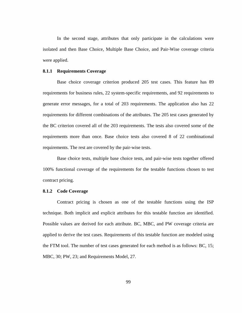
In the second stage, attributes that only participate in the calculations were
isolated and then Base Choice, Multiple Base Choice, and Pair-Wise coverage criteria
were applied.
8.1.1 Requirements Coverage
Base choice coverage criterion produced 205 test cases. This feature has 89
requirements for business rules, 22 system-specific requirements, and 92 requirements to
generate error messages, for a total of 203 requirements. The application also has 22
requirements for different combinations of the attributes. The 205 test cases generated by
the BC criterion covered all of the 203 requirements. The tests also covered some of the
requirements more than once. Base choice tests also covered 8 of 22 combinational
requirements. The rest are covered by the pair-wise tests.
Base choice tests, multiple base choice tests, and pair-wise tests together offered
100% functional coverage of the requirements for the testable functions chosen to test
contract pricing.
8.1.2 Code Coverage
Contract pricing is chosen as one of the testable functions using the ISP
technique. Both implicit and explicit attributes for this testable function are identified.
Possible values are derived for each attribute. BC, MBC, and PW coverage criteria are
applied to derive the test cases. Requirements of this testable function are modeled using
the FTM tool. The number of test cases generated for each method is as follows: BC, 15;
MBC, 30; PW, 23; and Requirements Model, 27.
99

Table 44: Case Study #1 - Statement Coverage Results
Base Choice
Multiple Base
Choice Pair-Wise Pair-Wise
– Refined Requirements
Model
Number of Tests 15 30 23 23 27 SwapContractService Coverage
86% 92% 85% 92% 92%
SwapContractCalculator Coverage
85% 90% 79% 90% 82%
The following 6 Java programs contain the logic for this case study. The LOC for each
program appear in the parenthesis.
1. SwapBUBDDetail.java – (461 LOC)
2. SwapContractCalculator.java – (166 LOC)
3. SwapContractService.Java – (258 LOC)
4. SwapDetailPriceResult.java – (757 LOC)
5. SwapPriceResult.java – (1343 LOC)
6. SwapService.java – (4040 LOC)
In the above programs, program # 1 gets the inputs for calculations from buy-up and buy-
down (BUBD) grids. Program # 3 gets pricing attributes for the contract from LPC
subsystem. Program # 4 displays the pricing results on the user interface and # 5 save the
results in the database. Program # 6 distinguishes the swap contracts from cash contracts.
100

In addition, there are other files in which contract attributes are defined and are
initialized. There are also separate programs that are initialized to catch the exceptions
and throw the error messages defined in the XML files. The statement coverage is
measured on the programs 2 and 3.
The contract entity has 203 business rules defined for its 29 attributes. There are 16
programs to handle the logic for the business rules.
ISP is applied in 2 stages for this case study. In the first stage, all the business rules are
verified using BC coverage and PW-coverage. Since this scope is not part of the
calculation engines, only the functional coverage of the tests is mentioned and not the
structural coverage.
The statement coverage achieved by the test cases from each method is shown in Table
44
8.1.3 Observations
Base choice coverage achieved good coverage of the functional requirements for
the characteristics defined for each and every attribute. Characteristics of these attributes
are validated at the client layer of the application, which means that the application filters
any invalid values for each attribute, before saving the entity in the database. This may
not be true in all cases, as the data for calculations will be received from external systems
that were implemented decades ago and may be defective.
Contracts are fundamentally of three types: Fixed Contract, Balloon Contract, or
ARM Contract. Fixed and Balloon contracts possess the same characteristics. Therefore,
101

the MBC criterion is applied by choosing the value for Contract type as “Fixed” in base
test #1 and “ARM” in base test # 2.
When the implementation is inspected, the information flow for the Fixed and
ARM Contracts is the same for the most part. This is also clear from the coverage results,
as BC offered 86% of the coverage and MBC offered 92% of the coverage.
When the PW criterion was applied, the program generated the test cases with
“default” or “do not care” values after all the combinations of that attribute with others
were fulfilled. When a default value is accepted as the input, the coverage is 82%. When
the default value was replaced test case #16 by “FIXED,” it achieved 91% coverage.
When the individual characteristics of each attribute need to be tested, BC test
cases offer good coverage of the functional requirements. It is relatively easy to trace the
test cases to the requirements, as each characteristic defined for the attribute will have
one test case from BC.
The PW criterion does not help when the characteristics have a large number of
attributes because it is difficult to map the PW test cases to the requirements where
traceability is an important factor to determine the coverage. Using pair-wise is also
cumbersome, because mapping tests to the requirements is hard with too many partitions.
The pair-wise criterion definitely helps in reducing or eliminating the duplicate pairs of
inputs and hence is used to eliminate the constraints that do not coexist. If the
implementation is such that it will not allow these combinations to be input, then almost
all of the pair-wise tests become infeasible from a design perspective. Grindal, Offutt,
and Mellin (2006) proposed a submodel strategy to handle the constraints between the
102

partitions. Later, I found it is more helpful than the pair-wise strategy. As mentioned
earlier, this case study is tested in 2 stages. In the first stage only, out of 230
requirements, base choice did not cover 16 requirements. Pair-wise covered these 16
requirements, but it took a very long time to filter these 16 from 172 pair-wise tests.
Instead of applying the pair-wise criterion, a submodel strategy would have helped.
8.2 Case Study #2: Loan Pricing
The ISP method is applied to determine the testable functions for the Loan Pricing
feature. The testable function in this feature has the following three entities involved:
Loan, Contract, and Master Commitment, which have 140, 29, and 35 attributes
respectively. Out of these only 6 attributes contribute to the calculations. BC, MBC, and
PW coverage criteria are applied to generate the test cases. The requirements of this
testable function are also modeled using the FTM tool. Coverage of these test cases
against the requirements as well as code are described in the following sections.
8.2.1 Requirements Coverage
Loan pricing functionality in this case study is captured in the form of a use case
that has one main flow, one alternate flow, and three exception flows. Other flows are
ignored for this case study. BC, MBC, and PW together covered 100% of the functional
requirements.
8.2.2 Code Coverage
Logic for loan pricing was captured in three Java classes namely,
SwapLoanService.java, SwapLoanCalculator.Java, and SwapLoanBase.java. The LOC
for each program are 549, 194, and 139 respectively.
103

A method priceLoan () was added to SwapLoanService.java to receive the inputs
directly from the spreadsheet. Parasoft’s jTest tool was used to determine the code
coverage. The test configuration was created in the tool that takes the inputs from
spreadsheet. The tests were run using the inputs from BC, MBC, PW, and Requirements
Modeling. Java classes were modified/commented without altering the behavior of the
programs. Code coverage is shown in Table 45.
Table 45: Case Study #2 - Statement Coverage Results
Base Choice Multiple Base Choice Pair-Wise Requirements
Model Number of Tests 26 52 72 131 Statement Coverage 86% 89% 92% 97%
8.2.3 Observations
Requirements coverage achieved by the BC and MBC are quite different, as the
loans are broadly classified as Fixed loans and ARM loans. Even though they share some
functional requirements, they are duplicated for the most part. Therefore, functional
coverage by the BC tests and the MBC tests are very different, even though code
coverage on same tests was only slightly higher with the MBC tests.
Attributes that are chosen in this testable function have a number of constraints.
The PW tests had good coverage, but have a lot of test cases when compared to BC. To
manually determine which pair-wise tests actually filled the gaps left by base choice
coverage took very long time.
104

The requirements model generated 131 test cases. Most of these test cases are
redundant because the same flow of the information is duplicated for Fixed, ARM, and
Balloon contracts. In the requirements modeling, the testable function chosen has more
scope than the function considered for ISP.
8.3 Case Study #3
The testable function of the Amortization feature has very distinct characteristics.
For each loan or instrument, the system should generate amortized payments for every
month until the end of the loan’s life. This testable function involves a series of
calculations that occur sequentially; output of one calculation is sent to the next
calculation. When this testable function is considered, loops are isolated and tested
separately. The loop characteristics are considered as a separate testable function and are
tested separately.
8.3.1 Requirements Coverage
Base choice tests had good functional requirements coverage: 100% of the
functional requirements are covered with base choice tests.
8.3.2 Code Coverage
The base choice tests had statement coverage of 100%, as shown in Table 46.
The logic in this case study is captured in seven programs. It was relatively easy to
isolate the programs, as this is the new system. Among the seven programs, three are
related to declaration, initialization, and obtaining the data from the external systems.
Two programs capture the logic of persisting the amortized data to the database. The
105

remaining two programs compute the amortization on different conditions. These two
programs had 1733 and 1521 LOC.
This entire application has ~80K LOC. This application has 630 base
choice tests for the entire functionality.
Table 46: Case Study #3 - Statement Coverage Results
Base Choice Multiple Base choice Pair-Wise Requirements
Model Number of Tests 74 N/A N/A N/A Statement Coverage 100% 0 0 0
8.3.3 Observations
This case study contains 16 different calculations that occur sequentially to
generate the final result. I did this case study in two ways: (a) all 16 calculators are
wrapped in a single testable function, and (b) each calculator is considered as one testable
function.
In the first case, I applied base choice, pair-wise, and multiple base choice
criteria. Each criterion achieved 20, 41, and 36 tests and 81%, 81%, and 68% of the
statement coverage. Although the pair-wise has a greater number of tests, they resulted in
infeasible tests. However, this method of choosing the testable function is not correct in
this type of calculation application.
106

In the second case, I applied base choice criteria to all 16 testable functions. The
74 base choice tests not only achieved 100% functional coverage on requirements, but
also achieved 100% statement coverage.
8.4 Case Study #4
Specifications for this case study are very typical for the calculation engines as
discussed in Chapter 2 Section 2.4. Amortization calculations in this case study are
similar to those of Case Study #3. The framework recommended in the Chapter 10 of this
thesis is applied to validate whether the steps defined in the framework provide proper
guidance in applying ISP. The base choice tests alone offered the required coverage of
the requirements. Therefore, multiple base choice coverage and pair-wise coverage were
not applied.
8.4.1 Requirements Coverage
Base choice tests achieved 100% functional coverage of the requirements. The 8
testable functions have a total number of 32 base choice tests. The testable functions TF
#5, 6, 7, and 8 should be tested at different periods of the loop conditions. Therefore, 8
base choice tests of these testable functions should be repeated at the initial period, first
period, current period, and the final period of the loan instrument and they result in 32
tests. These 32 tests are in addition to 24 base choice tests of the testable functions TF #1,
2, 3, and 4, which covered all the functional requirements within the scope.
8.4.2 Code Coverage
Code coverage is summarized in Table 47.
107

The logic in this case study is captured in three programs, excluding the programs
to access the data from external systems and save it to the database after processing.
These programs have 212, 1243, and 119 LOC.
The total LOC is not known for this application.
Table 47: Case Study # 4 - Statement Coverage Results
Base Choice Multiple Base Choice Pair-Wise Requirements
Model Number of Tests 56 N/A N/A N/A Statement Coverage 100% 0 0 0
8.4.3 Observations
The 8 testable functions have a total of 32 base choice tests. The testable
functions TF #5, 6, 7, and 8 should be tested at different periods of the loop conditions.
Therefore, 8 base choice tests of these testable functions should be repeated at the initial
period, first period, current period, and the final period of the loan instrument and they
result in 32 tests.
The requirements were modeled with a different approach. The model produced
12 tests as shown in Appendix B. Because these test cases required a lot of rework in the
prefixing, later the idea of using the modeling to test this use case was dropped. However,
if the testable functions deduced in this case study are used for modeling, then modeling
would have certainly achieved good coverage.
108

The systematic/methodical application of the standard framework defined in this
thesis simplified the complexity in analyzing the requirements. Base choice coverage not
only achieved complete coverage on the requirements, but also achieved 100% statement
coverage on the code.
109

9 Advantage and Disadvantages
This chapter analyzes the results and observations of Chapter 8 and presents the
pros and cons of each method applied to test the calculation engines.
9.1 Pros and Cons of Modeling
Test models provide a straightforward representation of the requirements where a
testable function, particular response, or response subset is to be selected by evaluating
many related conditions. The test models are effective for revealing defects in their
implementation and their specification. They can also support test design at any scope,
from methods at the unit level to a system in its entirety. The FTM supports automated
generation of test cases. The following subsections explain the advantages and
disadvantages of modeling.
9.1.1 Advantages of Modeling
Requirements modeling using FTM instantly generates the test cases from the
model. When modeled early in the life cycle, the requirements provide the test
analyst an idea of the number of test cases that need to be tested, which can be
used to measure or estimate the time needed to test.
FTM helps to map the test cases to the requirements. The traceability of the
test cases to the specifications is simultaneously achieved along with the
modeling.
110

Audit requirements for the test cases are: (a) test cases should be repeatable,
(b) test cases should contain enough level of detail, and (c) test cases should
be mapped to the requirements. These 3 audit requirements are met using the
FTM.
FTM allows users to mark the critical paths in a tree. These paths help in
identifying the regression testing suite or the smoke-testing suite.
Models bring common understanding of the requirements among the business
analysts, the programmers, and the test analysts.
When the requirements are changed, and when the changes are applied to the
tests, the FTM is designed to highlight the impacted paths, easing impact
analysis.
When the relations or constraints among the attributes are modeled carefully,
modeling precludes unnecessary or infeasible combinations.
9.1.2 Disadvantages of Modeling
A model’s success largely depends on the following factors.
Skill set: Modeling requires the personnel to understand software engineering
concepts in order to be efficient. For example, if the test analysts understand
different UML diagrams, it helps them to transform use cases, sequence
diagrams, and activity diagrams into test models using FTM, which in turn
helps them to derive test cases. In an environment where all the resources
including business analysts are used to conduct testing, it is optimal to expect
the required skill set.
111

Domain knowledge: The effectiveness of the test model largely depends on
the domain knowledge of the test analysts. For example, in Case Study #1 and
Case Study #2, the requirements state that a calculator should pull the price
values from grids. In this case, if the test analyst understands the domain and
nature of the application, this step can be ignored in modeling. It is difficult to
decide what to model and what to omit from modeling unless the modelers are
experienced and trained.
Model’s inconsistency: In spite of the guidance on modeling, different test
analysts model the same requirements differently. In some cases test analysts
are obsessed with modeling, leading them to modeling analysis paralysis.
Analysis Paralysis is a term given to the situation where a team of otherwise
intelligent and well-meaning analysts enters into a phase of analysis that only
ends when the project is cancelled (Analysis Paralysis). In Case Study #2
users were unable to confine themselves to the scope of the testable function.
The model generated 131 test cases, but most of them are redundant.
Consistency in practice: In large organizations, a consistent way of developing
the software is very important. Freddie Mac is hugely disadvantaged by
accounting mistakes in the past. The methodology and controls insist on
consistency in practice. Any new tool has to complement the existing tools.
TestManager is used to manage the test cases. Test cases generated by FTM
have to be translated into a format that the TestManager tool can understand.
Changes in requirements leads to changes in the test models, and therefore
112

changes in test cases. This incurred an extra burden on the teams. Flux in the
requirements also leads to problems in maintaining the models. These
problems lead to less management support.
9.2 Pros and Cons of ISP
Case studies are discussed in Chapters 4, 5, 6, and 7. Chapter 8 details the results
and observations of the case studies. The following section explains the pros and cons of
the ISP technique.
9.2.1 Advantages of ISP
Test analysts are knowledgeable about the fundamentals of the equivalence
partitioning, boundary value analysis, error guessing and other techniques of
black box testing. The ISP technique can easily be understood with such a
background.
ISP gives good guidance when deriving the testable functions: Steps defined
in the recommended framework provide clear guidance on how to isolate the
set of requirements that can form a testable function. This method of
exploring the requirements unfolds the complexity in an application. For
example, in Case Study #4, although calculations appear to be receiving the
inputs from four different external systems, this analysis of identifying the
testable function simplified the complex look of the requirements.
Test cases to satisfy different coverage criteria are automated. What is
established with the help of case studies is the fact that these test cases, when
executed, achieved good coverage of the requirements as well as the statement
113

coverage. This coverage provided more assurance to adapt this framework and
implement the suggested approach.
Test cases can be generated early in the cycle. Soon after the objects are
identified, entities are defined, and their relations are specified, test case
design can be started using this approach. In Case Study #2, test analysts
designed and completed the test cases even before developers completed
coding the requirements. Developers used these tests to test their
implementation in addition to their unit tests. When system testing is
conducted, fewer functional defects were found.
It is easy to trace BC and MBC test cases to the requirements, which is the
essential part of Freddie Mac’s methodology.
Freddie Mac’s methodology requires test cases to be repeatable, contain
enough level of detail, and then they should be mapped to the requirements.
Test cases derived using this technique satisfy the methodology requirements.
The majority of the applications in Freddie Mac, or any other financial
service, are data intensive, which means the same scenario may need to be
executed by multiple sets of data. For example, Freddie Mac has hundreds of
products for Fixed and ARM categories. All of the products in each category
share most of their properties and differ in some. In many test cases derived
using the BC and MBC, the same requirement is covered more than once. In
this case, when the test cases need prefixing of the values, they are varied with
114

different products. Therefore, not only are requirements well covered, but
tests have a rich variety in data.
Controllability: The case studies discussed in this thesis show that test cases
derived using ISP offer good coverage not only of the requirements but also
on the code.
Observability: When there are multiple calculations occurring in a series or in
parallel, all the requirements are broken into multiple testable functions for
each calculation. While generating the expected results, all the intermediate
values of the attributes are logged. The test team suggested the development
team follow the same approach, which means to save the intermediate values
of these variables into traces, while persisting the final values in the database.
This approach simplified the process of diagnosing the differences in expected
and actual results.
Data aging: Test data that is used for one reporting cycle may not be useful for
another reporting cycle. For example, when a loan is created in the system in
January with the settlement date in April, the same loan data cannot be reused
to test the February month cycle. This problem is called data aging. In test
case design, only abstract values are used so that actual values can be applied
periodically and with the current data. Automation is also applied to keep the
data current. This approach simplified and resolved the data aging problem by
keeping the test case design abstract from passing the real values during the
test case design.
115

Changes in requirements: When the requirements were changed, the
traceability matrix allowed test analysts to quickly identify the impacted test
cases. As the entire process of test case design was automated, it became easy
to quickly generate a new set of test cases. The test analyst needed to simply
identify the impacted testable function, change the partitions and/or values in
the blocks to reflect the changes in requirements, and follow through the test
case design steps.
Submodeling: If the constraints among the attributes in a testable function
span more than 2 attributes and their relations are complex in nature, then any
one of the following actions can be taken to reduce the complexity: (a) the
testable function can be further separated into small testable functions, or (b) a
subset of attributes in the testable function can be chosen to apply the
coverage criteria in the first stage, and in the second stage outputs of the first
stage can be tested in conjunction with the outputs of the second stage
(Grindal, Offutt, & Mellin, 2006).
Business rules: A business rule is a requirement that is expressed in non-
procedural and non-technical form, which implies specific constraints on data
or business processes (i.e. valid values, calculations, timing ranges, etc.). The
base choice criterion is best suited to test the business rules. For example, in
Case Study #1, there are 180 business rules to test in a feature. The first part
of the case study demonstrates how effective and efficient ISP was at testing
the business rules. In another instance, where there are 1359 business rules,
116

application of BC coverage criterion coupled with automation reduced the
testing cycle time from 5 business days to less than 2 hours. Also, the
maintenance time was reduced drastically.
Business cycles testing: In some applications, all the calculations in an
application need to be tested for different business cycles: weekly, monthly,
quarterly, and annually. Test data, along with the environment, needs to be
changed to simulate these cycles. The ISP technique with automation offered
this dynamism with the test data, keeping the process compliant with audit
requirements.
9.2.2 Disadvantages of ISP
The success of ISP largely depends on how well the testable functions are
identified and how discrete they are. For example, Case Study #3 considered
all the calculators as 1 single testable function instead of 11 testable functions.
When these 11 calculations are considered as individual testable functions,
they become very simple and straightforward. Case Study #4 demonstrates the
effectiveness of choosing testable function at a unit level.
ISP generates a large number of test cases across the entire application. ISP is
more efficient if complemented by automation.
The pair-wise criterion needs to be chosen carefully, otherwise more tests will
be invalid. It is difficult to determine which tests are invalid.
117

10 Conclusions and Recommendations
10.1 Conclusion
Calculation engines are similar in their characteristics with respect to their
specifications, architecture, and implementation. In this thesis’s case studies, a common
observation is that not all the attributes of the entities are important for the calculations.
Problem analysis is the first step in finding the solution, and identifying the testable
functions is a critical part in the problem analysis. Complexity in testing the calculations
can be reduced by identifying the testable functions that are part of the calculations. A
testable function can be a single requirement or a set of requirements that can be tested as
a single unit. Each testable function should be independent of the other and should be
testable in isolation. Functional and structural coverage of the requirements largely
depends on the identified testable functions.
The framework recommended in Section 10.2 explains a way to identify the
testable functions. Using automation, these sets of testable functions can be executed at
once.
Thus, this thesis proposes a framework to test calculation engines. The framework
provides guidance on deriving the testable functions and deriving the test cases. Case
studies demonstrated the effectiveness of the approach by using common applications in
the calculation engines and covering different characteristics.
118

• Case Study #1 explains how to isolate and test the calculation engines at
different layers.
• Case Study #2 demonstrates how to analyze and simplify the calculation
requirements and then how to test them.
• Case Study #3 demonstrates testing the very common amortization application
in the financial services industry using ISP and automation.
• Case Study #4 shows a practical application of this framework.
This thesis began with addressing the problem with the help of modeling
requirements. Although comparing the results of modeling with ISP was not an initial
goal, the ISP technique was found to be better and to produce more consistent results.
The outcome of the modeling approach largely depends on the skill set of the test analyst.
Systematic application of the technique to the problem is necessary. All four case
studies confirm that BC and MBC, if applied according to the steps defined in the
framework, offer good functional and structural coverage. It was also found that BC and
MBC cover a large number of combinations among the attributes.
In the case studies # 1 and # 2, the statement coverage gaps, are traced to the
exceptions. Programs handle the additional exceptions that are not in the scope of the
functionality under tests. But when inputs are derived using ISP, blocks for the
exceptions are not considered, as these exceptions are already filtered in the client layer.
The FTM framework is best applicable at the integration, system, and user
acceptance test levels. In Case Study #3, test inputs were derived in advance to the
coding and were given to the development team to satisfy these tests. This helped
119

improve the software, as there were relatively few functional defects observed during
system testing.
Tests derived following this framework and using the BC or MBC coverage
criterion offer simple traceability to the requirements, which is an important requirement
in the Freddie Mac’s methodology.
This framework can easily be adapted to different development methodologies
such as waterfall, spiral model, and RAD.
In all the cases examined, this framework not only proved to be effective in terms
of coverage, but also very efficient. In Case Study #3, the entire application has 11 use
cases and the total number of tests is close to 600. The application first runs with these
600 tests with a clean pass. Subsequently this application is tested with monthly cycle
data that has 17,000 records with 0 defects. This entire process eventually was reduced to
0.5 days from 5 days.
10.2 Recommendations
The following framework, when used to test the calculation engines using the ISP
technique, achieved consistency and offered repeatability. The steps below describe the
process framework to test the calculation engines and extend the category partition
method framework defined by Ostrand and Balcer (1998).
Step 1 Problem analysis is a crucial part of the ISP. In the first step, identify the
problem to be addressed.
Step 2 Identify the testable functions. The testable functions could be a
calculation set, a characteristic of a single attribute, a set of
120

characteristics of multiple attributes that can be tested together, a set of
conditions that triggers calculations, or a set of combination of values
that triggers calculations.
Step 3 Identify explicit and the implicit attributes of the testable function. Many
entities may take part in the testable function, but only a few attributes
influence the objective of the testable function.
Step 4 Identify all the possible distinct values that are both valid and invalid for
each attribute. Design specifications for the attributes of the testable
function can help identify these values. In this step, real values may not
be possible to consider. Therefore, any abstract values such as < 0, >0,
and =0 can be chosen as distinct values. Amortization calculations occur
recursively until the end of their term. Derive the blocks for loop
characteristics carefully. In addition, Grindal and Offutt’s (2007)
guidance on choosing the distinct values for the blocks using
equivalence partitioning and boundary value analysis helps in
determining the values.
Step 5 Apply the BC criteria with the invalid values and to derive the test cases
to test all the error conditions.
Step 6 After testing the invalid conditions, eliminate the invalid values from
each partition.
Step 7 Apply base choice, multiple base choice, and pair-wise coverage criteria
appropriately to the remaining valid values of each partition to generate
121

test cases with the valid values. Constraints may exist among these valid
values. If the constraints exist only between 2 partitions, then base
choice criterion covers critical constraints. If constraints exist among
more than 2 partitions, then pair-wise criterion helps in reducing the
number of tests, but it is very cumbersome to identify which
combinations are valid. Grindal, Offutt, and Mellin (2006) suggested
different strategies for conflict handling. The submodels strategy is
relatively simple and easy to apply, and can be used in place of the pair-
wise criterion to test the constraints among the partitions.
Step 8 Analyze requirements in the testable function and then identify the
constraints among the partitions. These constraints can be of two types:
either two or more attributes can coexist together with certain values, or
they do not coexist.
Step 9 Test cases derived in Step 7 should be manually inspected for the
conditions described in Step 8. Test cases that cannot be used should be
excluded from the test suite or can be included as negative test cases.
Step 10 Ensure that test cases cover all the functional requirements in the
testable function with the help of the Requirements Traceability Matrix
(RTM). Each requirement can be covered by more than one test case by
applying different coverage criteria as mentioned in Step 7. If the
coverage is not sufficient, then choose more values for each partition
and repeat from Step 3 to Step 10.
122

Step 11 Prefix the test cases with other attribute values that are trivial in this
testable function but are required to execute the test case. In Step 3, if
any of the other trivial attributes of the entities that are excluded in
deriving the test cases are described in Step 7, prefix the test cases with
these excluded attributes.
Step 12 Provide the real values for each attribute of the test cases, in place of
arbitrary values chosen in the Step 3. Now the test case becomes
executable.
Step 13 Build the calculation simulator, and then execute the test cases against
the simulator to derive expected results.
Step 14 Execute the test cases against the system-under-test and get the actual
results.
Step 15 Compare actual results with expected results to determine whether the
test case passes or fails.
10.3 Further Work
10.3.1 Automatic Generation of Test Data for ISP tests
Abstract values are used to generate the ISP tests. Later, real values are added in
place of arbitrary values. If the ranges of values for each partition/block and their
constraints of other values in different partitions/blocks are known, then automatic test
data generation is possible. If the automation is coupled with auto generation of the test
data, this will further improve the efficiency of testing the calculation engines.
123

10.3.2 Filter the Conflicting Combinations Automatically
In the first two case studies, the pair-wise criterion is applied to derive the
combinatorial tests. In both the cases, a number of pair-wise tests are invalid and more
time is spent in filtering the valid tests from the pair-wise tests. I found it is more efficient
to apply the submodels strategy instead of pair-wise tests. Grindal, Offutt, and Mellon
(2006) discussed several strategies in managing the conflicts. The dependencies or
conflicts between the partitions can be identified and the tests can be filtered accordingly
using the automation.
10.3.3 Build the Tool With a User Interface
A Java utility was written to automatically generate the Base Choice and Multiple
Base Choice test cases. Bach’s PERL program is used to generate the pair-wise tests.
These utilities read the inputs from spreadsheet and write the outputs to spreadsheet or a
word processor. Freddie Mac’s methodology requires proper documentation of the
practice. A tool with the help of a user interface to define the partitions, blocks, and input
the values will greatly enhance and ease the process of deriving the test inputs. This
approach can then be incorporated in their test strategy.
10.3.4 Auto Detection of the Requirements Coverage and Building Traceability
Requirements within the scope of testing can be divided into multiple testable
functions. When a testable function is chosen to derive the test inputs, and if the
corresponding requirement numbers are associated with each test input, then functional
coverage of the requirements can be analyzed. For example, Bach’s PERL program
generates the test inputs along with the pairs of attributes that are covered in each test
124

input. When the same requirement is covered multiple times, it will help in varying the
values of the inputs. For example, when the partition “product type” is covered multiple
times, different products—30 Y FIXED, 40 Y FIXED, etc.—are passed as real values.
This not only improves coverage, but also provides rich variation in the test data. At
present, this identification is done manually. Automating this detection of the coverage
could greatly enhance the testing efficiency.
10.3.5 Testable Functions as an Estimation Technique
Test analysts are able to quickly identify the testable functions after analyzing a
few use cases or a subset of the requirements. They are also able to recognize the testable
functions that can be tested and executed together. Derived testable functions can be
categorized as low, medium, and high by the number of characteristics of each attribute
and constraints among the attributes. It is possible to predict the number of test inputs for
each testable function. This information, if obtained early in the life cycle of the project,
could help estimate the testing efforts of the project.
125

Appendix A. Modeling Outputs for Case Study # 1
125

126

127

128

129
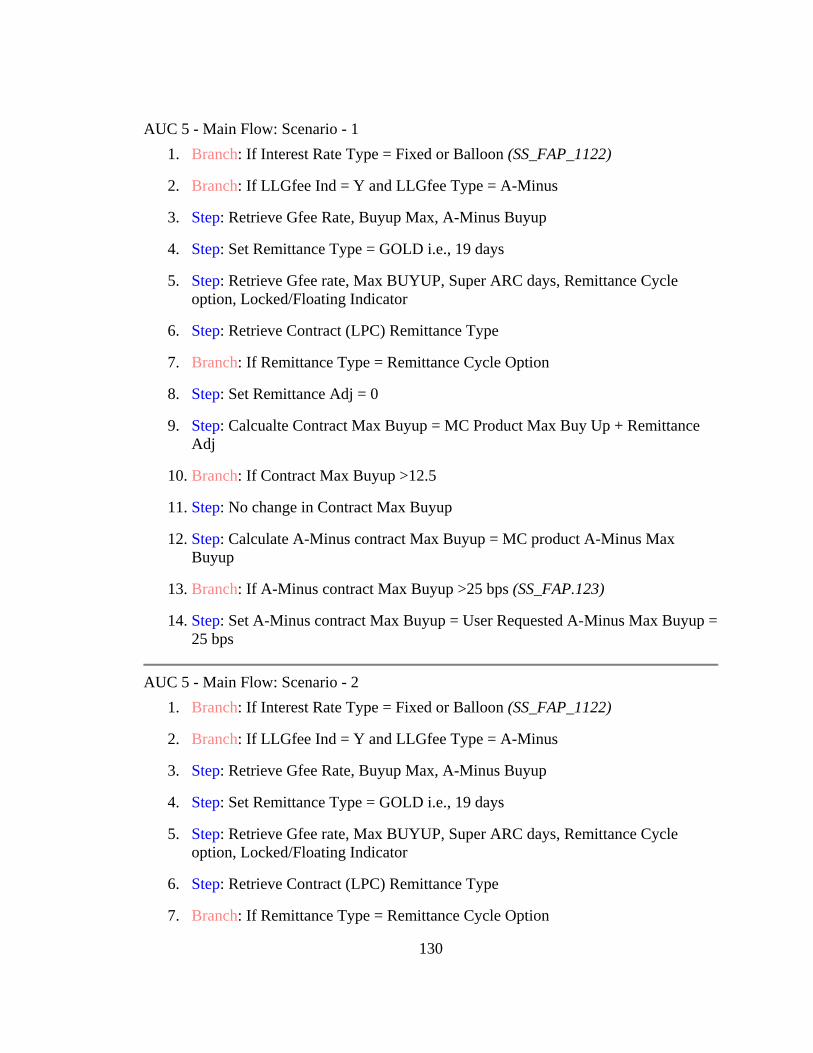
AUC 5 - Main Flow: Scenario - 1 1. Branch: If Interest Rate Type = Fixed or Balloon (SS_FAP_1122)
2. Branch: If LLGfee Ind = Y and LLGfee Type = A-Minus
3. Step: Retrieve Gfee Rate, Buyup Max, A-Minus Buyup
4. Step: Set Remittance Type = GOLD i.e., 19 days
5. Step: Retrieve Gfee rate, Max BUYUP, Super ARC days, Remittance Cycle option, Locked/Floating Indicator
6. Step: Retrieve Contract (LPC) Remittance Type
7. Branch: If Remittance Type = Remittance Cycle Option
8. Step: Set Remittance Adj = 0
9. Step: Calcualte Contract Max Buyup = MC Product Max Buy Up + Remittance Adj
10. Branch: If Contract Max Buyup >12.5
11. Step: No change in Contract Max Buyup
12. Step: Calculate A-Minus contract Max Buyup = MC product A-Minus Max Buyup
13. Branch: If A-Minus contract Max Buyup >25 bps (SS_FAP.123)
14. Step: Set A-Minus contract Max Buyup = User Requested A-Minus Max Buyup = 25 bps
AUC 5 - Main Flow: Scenario - 2
1. Branch: If Interest Rate Type = Fixed or Balloon (SS_FAP_1122)
2. Branch: If LLGfee Ind = Y and LLGfee Type = A-Minus
3. Step: Retrieve Gfee Rate, Buyup Max, A-Minus Buyup
4. Step: Set Remittance Type = GOLD i.e., 19 days
5. Step: Retrieve Gfee rate, Max BUYUP, Super ARC days, Remittance Cycle option, Locked/Floating Indicator
6. Step: Retrieve Contract (LPC) Remittance Type
7. Branch: If Remittance Type = Remittance Cycle Option
130

8. Step: Set Remittance Adj = 0
9. Step: Calcualte Contract Max Buyup = MC Product Max Buy Up + Remittance Adj
10. Branch: If Contract Max Buyup >12.5
11. Step: No change in Contract Max Buyup
12. Step: Calculate A-Minus contract Max Buyup = MC product A-Minus Max Buyup
13. Branch: If A-Minus contract Max Buyup <=25 bps
14. Step: Set User requested A-Minus Buyup = Calculated contract A-Minus Max Buyup
AUC 5 - Main Flow: Scenario - 3
1. Branch: If Interest Rate Type = Fixed or Balloon (SS_FAP_1122)
2. Branch: If LLGfee Ind = Y and LLGfee Type = A-Minus
3. Step: Retrieve Gfee Rate, Buyup Max, A-Minus Buyup
4. Step: Set Remittance Type = GOLD i.e, 19 days
5. Step: Retrieve Gfee rate, Max BUYUP, Super ARC days, Remittance Cycle option, Locked/Floating Indicator
6. Step: Retrieve Contract (LPC) Remittance Type
7. Branch: If Remittance Type = Remittance Cycle Option
8. Step: Set Remittance Adj = 0
9. Step: Calcualte Contract Max Buyup = MC Product Max Buy Up + Remittance Adj
10. Branch: If Contract Max Buyup <=12.5
11. Step: Contract Max BuyUp = User Requested Max Buyup = MC Product Max Buyup = 12.5bps
12. Step: Calculate A-Minus contract Max Buyup = MC product A-Minus Max Buyup
13. Branch: If A-Minus contract Max Buyup >25 bps
131

14. Step: Set A-Minus contract Max Buyup = User Requested A-Minus Max Buyup = 25 bps
AUC 5 - Main Flow: Scenario - 4
1. Branch: If Interest Rate Type = Fixed or Balloon (SS_FAP_1122)
2. Branch: If LLGfee Ind = Y and LLGfee Type = A-Minus
3. Step: Retrieve Gfee Rate, Buyup Max, A-Minus Buyup
4. Step: Set Remittance Type = GOLD i.e, 19 days
5. Step: Retrieve Gfee rate, Max BUYUP, Super ARC days, Remittance Cycle option, Locked/Floating Indicator
6. Step: Retrieve Contract (LPC) Remittance Type
7. Branch: If Remittance Type = Remittance Cycle Option
8. Step: Set Remittance Adj = 0
9. Step: Calcualte Contract Max Buyup = MC Product Max Buy Up + Remittance Adj
10. Branch: If Contract Max Buyup <=12.5
11. Step: Contract Max BuyUp = User Requested Max Buyup = MC Product Max Buyup = 12.5bps
12. Step: Calculate A-Minus contract Max Buyup = MC product A-Minus Max Buyup
13. Branch: If A-Minus contract Max Buyup <=25 bps
14. Step: Set User requested A-Minus Buyup = Calculated contract A-Minus Max Buyup
AUC 5 - Main Flow: Scenario - 5
1. Branch: If Interest Rate Type = Fixed or Balloon (SS_FAP_1122)
2. Branch: If LLGfee Ind = Y and LLGfee Type = A-Minus
3. Step: Retrieve Gfee Rate, Buyup Max, A-Minus Buyup
4. Step: Set Remittance Type = GOLD i.e, 19 days
132

5. Step: Retrieve Gfee rate, Max BUYUP, Super ARC days, Remittance Cycle option, Locked/Floating Indicator
6. Step: Retrieve Contract (LPC) Remittance Type
7. Branch: If Remittance Type <> Remittance Cycle Option
8. Branch: If Remittance Option is Floating
9. Step: Retrive One day float value from Pricing parameter Table using pooling prod. Id float type and contract date
10. Step: Calculate Remittance Adj = (Default Remittance days based on the product - P/I No. of days)* float value
11. Step: Calculate Contract Adjusted Gfee = Base Gfee Rate - Remitence Adj
12. Step: Calcualte Contract Max Buyup = MC Product Max Buy Up + Remitence Adj
13. Branch: If Contract Max Buyup >12.5
14. Step: No change in Contract Max Buyup
15. Step: Calculate A-Minus contract Max Buyup = MC product A-Minus Max Buyup
16. Branch: If A-Minus contract Max Buyup >25 bps
17. Step: Set A-Minus contract Max Buyup = User Requested A-Minus Max Buyup = 25 bps
AUC 5 - Main Flow: Scenario - 6
1. Branch: If Interest Rate Type = Fixed or Balloon (SS_FAP_1122)
2. Branch: If LLGfee Ind = Y and LLGfee Type = A-Minus
3. Step: Retrieve Gfee Rate, Buyup Max, A-Minus Buyup
4. Step: Set Remittance Type = GOLD i.e, 19 days
5. Step: Retrieve Gfee rate, Max BUYUP, Super ARC days, Remittance Cycle option, Locked/Floating Indicator
6. Step: Retrieve Contract (LPC) Remittance Type
7. Branch: If Remittance Type <> Remittance Cycle Option
133

8. Branch: If Remittance Option is Floating
9. Step: Retrive One day float value from Pricing parameter Table using pooling prod. Id float type and contract date
10. Step: Calculate Remittance Adj = (Default Remittance days based on the product - P/I No. of days)* float value
11. Step: Calculate Contract Adjusted Gfee = Base Gfee Rate - Remitence Adj
12. Step: Calcualte Contract Max Buyup = MC Product Max Buy Up + Remitence Adj
13. Branch: If Contract Max Buyup >12.5
14. Step: No change in Contract Max Buyup
15. Step: Calculate A-Minus contract Max Buyup = MC product A-Minus Max Buyup
16. Branch: If A-Minus contract Max Buyup <=25 bps
17. Step: Set User requested A-Minus Buyup = Calculated contract A-Minus Max Buyup
AUC 5 - Main Flow: Scenario - 7
1. Branch: If Interest Rate Type = Fixed or Balloon (SS_FAP_1122)
2. Branch: If LLGfee Ind = Y and LLGfee Type = A-Minus
3. Step: Retrieve Gfee Rate, Buyup Max, A-Minus Buyup
4. Step: Set Remittance Type = GOLD i.e, 19 days
5. Step: Retrieve Gfee rate, Max BUYUP, Super ARC days, Remittance Cycle option, Locked/Floating Indicator
6. Step: Retrieve Contract (LPC) Remittance Type
7. Branch: If Remittance Type <> Remittance Cycle Option
8. Branch: If Remittance Option is Floating
9. Step: Retrive One day float value from Pricing parameter Table using pooling prod. Id float type and contract date
10. Step: Calculate Remittance Adj = (Default Remittance days based on the product - P/I No. of days)* float value
134

11. Step: Calculate Contract Adjusted Gfee = Base Gfee Rate - Remitence Adj
12. Step: Calcualte Contract Max Buyup = MC Product Max Buy Up + Remitence Adj
13. Branch: If Contract Max Buyup <=12.5
14. Step: Contract Max BuyUp = User Requested Max Buyup = MC Product Max Buyup = 12.5bps
15. Step: Calculate A-Minus contract Max Buyup = MC product A-Minus Max Buyup
16. Branch: If A-Minus contract Max Buyup >25 bps
17. Step: Set A-Minus contract Max Buyup = User Requested A-Minus Max Buyup = 25 bps
AUC 5 - Main Flow: Scenario - 8
1. Branch: If Interest Rate Type = Fixed or Balloon (SS_FAP_1122)
2. Branch: If LLGfee Ind = Y and LLGfee Type = A-Minus
3. Step: Retrieve Gfee Rate, Buyup Max, A-Minus Buyup
4. Step: Set Remittance Type = GOLD i.e, 19 days
5. Step: Retrieve Gfee rate, Max BUYUP, Super ARC days, Remittance Cycle option, Locked/Floating Indicator
6. Step: Retrieve Contract (LPC) Remittance Type
7. Branch: If Remittance Type <> Remittance Cycle Option
8. Branch: If Remittance Option is Floating
9. Step: Retrive One day float value from Pricing parameter Table using pooling prod. Id float type and contract date
10. Step: Calculate Remittance Adj = (Default Remittance days based on the product - P/I No. of days)* float value
11. Step: Calculate Contract Adjusted Gfee = Base Gfee Rate - Remitence Adj
12. Step: Calcualte Contract Max Buyup = MC Product Max Buy Up + Remitence Adj
13. Branch: If Contract Max Buyup <=12.5
135

14. Step: Contract Max BuyUp = User Requested Max Buyup = MC Product Max Buyup = 12.5bps
15. Step: Calculate A-Minus contract Max Buyup = MC product A-Minus Max Buyup
16. Branch: If A-Minus contract Max Buyup <=25 bps
17. Step: Set User requested A-Minus Buyup = Calculated contract A-Minus Max Buyup
AUC 5 - Main Flow: Scenario - 9
1. Branch: If Interest Rate Type = Fixed or Balloon (SS_FAP_1122)
2. Branch: If LLGfee Ind = Y and LLGfee Type = A-Minus
3. Step: Retrieve Gfee Rate, Buyup Max, A-Minus Buyup
4. Step: Set Remittance Type = GOLD i.e, 19 days
5. Step: Retrieve Gfee rate, Max BUYUP, Super ARC days, Remittance Cycle option, Locked/Floating Indicator
6. Step: Retrieve Contract (LPC) Remittance Type
7. Branch: If Remittance Type <> Remittance Cycle Option
8. Branch: If Remittance Option is Locked
9. Step: Retrive One day float value from GFEE Table using pooling prod. Id, float type and locked date
10. Step: Calculate Remittance Adj = (Default Remittance days based on the product - P/I No. of days)* float value
11. Step: Calculate Contract Adjusted Gfee = Base Gfee Rate - Remitence Adj
12. Step: Calcualte Contract Max Buyup = MC Product Max Buy Up + Remitence Adj
13. Branch: If Contract Max Buyup >12.5
14. Step: No change in Contract Max Buyup
15. Step: Calculate A-Minus contract Max Buyup = MC product A-Minus Max Buyup
16. Branch: If A-Minus contract Max Buyup >25 bps
136

17. Step: Set A-Minus contract Max Buyup = User Requested A-Minus Max Buyup = 25 bps
AUC 5 - Main Flow: Scenario - 10
1. Branch: If Interest Rate Type = Fixed or Balloon (SS_FAP_1122)
2. Branch: If LLGfee Ind = Y and LLGfee Type = A-Minus
3. Step: Retrieve Gfee Rate, Buyup Max, A-Minus Buyup
4. Step: Set Remittance Type = GOLD i.e, 19 days
5. Step: Retrieve Gfee rate, Max BUYUP, Super ARC days, Remittance Cycle option, Locked/Floating Indicator
6. Step: Retrieve Contract (LPC) Remittance Type
7. Branch: If Remittance Type <> Remittance Cycle Option
8. Branch: If Remittance Option is Locked
9. Step: Retrive One day float value from GFEE Table using pooling prod. Id, float type and locked date
10. Step: Calculate Remittance Adj = (Default Remittance days based on the product - P/I No. of days)* float value
11. Step: Calculate Contract Adjusted Gfee = Base Gfee Rate - Remitence Adj
12. Step: Calcualte Contract Max Buyup = MC Product Max Buy Up + Remitence Adj
13. Branch: If Contract Max Buyup >12.5
14. Step: No change in Contract Max Buyup
15. Step: Calculate A-Minus contract Max Buyup = MC product A-Minus Max Buyup
16. Branch: If A-Minus contract Max Buyup <=25 bps
17. Step: Set User requested A-Minus Buyup = Calculated contract A-Minus Max Buyup
AUC 5 - Main Flow: Scenario - 11
1. Branch: If Interest Rate Type = Fixed or Balloon (SS_FAP_1122)
137

2. Branch: If LLGfee Ind = Y and LLGfee Type = A-Minus
3. Step: Retrieve Gfee Rate, Buyup Max, A-Minus Buyup
4. Step: Set Remittance Type = GOLD i.e, 19 days
5. Step: Retrieve Gfee rate, Max BUYUP, Super ARC days, Remittance Cycle option, Locked/Floating Indicator
6. Step: Retrieve Contract (LPC) Remittance Type
7. Branch: If Remittance Type <> Remittance Cycle Option
8. Branch: If Remittance Option is Locked
9. Step: Retrive One day float value from GFEE Table using pooling prod. Id, float type and locked date
10. Step: Calculate Remittance Adj = (Default Remittance days based on the product - P/I No. of days)* float value
11. Step: Calculate Contract Adjusted Gfee = Base Gfee Rate - Remitence Adj
12. Step: Calcualte Contract Max Buyup = MC Product Max Buy Up + Remitence Adj
13. Branch: If Contract Max Buyup <=12.5
14. Step: Contract Max BuyUp = User Requested Max Buyup = MC Product Max Buyup = 12.5bps
15. Step: Calculate A-Minus contract Max Buyup = MC product A-Minus Max Buyup
16. Branch: If A-Minus contract Max Buyup >25 bps
17. Step: Set A-Minus contract Max Buyup = User Requested A-Minus Max Buyup = 25 bps
AUC 5 - Main Flow: Scenario - 12
1. Branch: If Interest Rate Type = Fixed or Balloon (SS_FAP_1122)
2. Branch: If LLGfee Ind = Y and LLGfee Type = A-Minus
3. Step: Retrieve Gfee Rate, Buyup Max, A-Minus Buyup
4. Step: Set Remittance Type = GOLD i.e, 19 days
138

5. Step: Retrieve Gfee rate, Max BUYUP, Super ARC days, Remittance Cycle option, Locked/Floating Indicator
6. Step: Retrieve Contract (LPC) Remittance Type
7. Branch: If Remittance Type <> Remittance Cycle Option
8. Branch: If Remittance Option is Locked
9. Step: Retrive One day float value from GFEE Table using pooling prod. Id, float type and locked date
10. Step: Calculate Remittance Adj = (Default Remittance days based on the product - P/I No. of days)* float value
11. Step: Calculate Contract Adjusted Gfee = Base Gfee Rate - Remitence Adj
12. Step: Calcualte Contract Max Buyup = MC Product Max Buy Up + Remitence Adj
13. Branch: If Contract Max Buyup <=12.5
14. Step: Contract Max BuyUp = User Requested Max Buyup = MC Product Max Buyup = 12.5bps
15. Step: Calculate A-Minus contract Max Buyup = MC product A-Minus Max Buyup
16. Branch: If A-Minus contract Max Buyup <=25 bps
17. Step: Set User requested A-Minus Buyup = Calculated contract A-Minus Max Buyup
AUC 5 - Main Flow: Scenario - 13
1. Branch: If Interest Rate Type = Fixed or Balloon (SS_FAP_1122)
2. Branch: If LLGfee Ind = N and LLGfee Type = Not A-Minus
3. Step: Retrieve Gfee Rate, Buyup Max
4. Step: Set Remittance Type = GOLD i.e, 19 days
5. Step: Retrieve Gfee rate, Max BUYUP, Super ARC days, Remittance Cycle option, Locked/Floating Indicator
6. Step: Retrieve Contract (LPC) Remittance Type
7. Branch: If Remittance Type = Remittance Cycle Option
139

8. Step: Set Remittance Adj = 0
9. Step: Calcualte Contract Max Buyup = MC Product Max Buy Up + Remitence Adj
10. Branch: If Contract Max Buyup >12.5
11. Step: No change in Contract Max Buyup
AUC 5 - Main Flow: Scenario - 14 1. Branch: If Interest Rate Type = Fixed or Balloon (SS_FAP_1122)
2. Branch: If LLGfee Ind = N and LLGfee Type = Not A-Minus
3. Step: Retrieve Gfee Rate, Buyup Max
4. Step: Set Remittance Type = GOLD i.e, 19 days
5. Step: Retrieve Gfee rate, Max BUYUP, Super ARC days, Remittance Cycle option, Locked/Floating Indicator
6. Step: Retrieve Contract (LPC) Remittance Type
7. Branch: If Remittance Type = Remittance Cycle Option
8. Step: Set Remittance Adj = 0
9. Step: Calcualte Contract Max Buyup = MC Product Max Buy Up + Remitence Adj
10. Branch: If Contract Max Buyup <=12.5
11. Step: Contract Max BuyUp = User Requested Max Buyup = MC Product Max Buyup = 12.5bps
AUC 5 - Main Flow: Scenario - 15
1. Branch: If Interest Rate Type = Fixed or Balloon (SS_FAP_1122)
2. Branch: If LLGfee Ind = N and LLGfee Type = Not A-Minus
3. Step: Retrieve Gfee Rate, Buyup Max
4. Step: Set Remittance Type = GOLD i.e, 19 days
5. Step: Retrieve Gfee rate, Max BUYUP, Super ARC days, Remittance Cycle option, Locked/Floating Indicator
140

6. Step: Retrieve Contract (LPC) Remittance Type
7. Branch: If Remittance Type <> Remittance Cycle Option
8. Branch: If Remittance Option is Floating
9. Step: Retrive One day float value from Pricing parameter Table using pooling prod. Id float type and contract date
10. Step: Calculate Remittance Adj = (Default Remittance days based on the product - P/I No. of days)* float value
11. Step: Calculate Contract Adjusted Gfee = Base Gfee Rate - Remitence Adj
12. Step: Calcualte Contract Max Buyup = MC Product Max Buy Up + Remitence Adj
13. Branch: If Contract Max Buyup >12.5
14. Step: No change in Contract Max Buyup
AUC 5 - Main Flow: Scenario - 16 1. Branch: If Interest Rate Type = Fixed or Balloon (SS_FAP_1122)
2. Branch: If LLGfee Ind = N and LLGfee Type = Not A-Minus
3. Step: Retrieve Gfee Rate, Buyup Max
4. Step: Set Remittance Type = GOLD i.e, 19 days
5. Step: Retrieve Gfee rate, Max BUYUP, Super ARC days, Remittance Cycle option, Locked/Floating Indicator
6. Step: Retrieve Contract (LPC) Remittance Type
7. Branch: If Remittance Type <> Remittance Cycle Option
8. Branch: If Remittance Option is Floating
9. Step: Retrive One day float value from Pricing parameter Table using pooling prod. Id float type and contract date
10. Step: Calculate Remittance Adj = (Default Remittance days based on the product - P/I No. of days)* float value
11. Step: Calculate Contract Adjusted Gfee = Base Gfee Rate - Remitence Adj
141
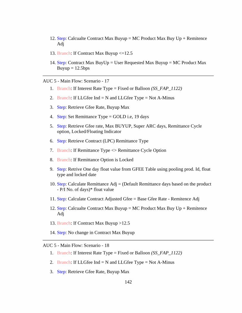
12. Step: Calcualte Contract Max Buyup = MC Product Max Buy Up + Remitence Adj
13. Branch: If Contract Max Buyup <=12.5
14. Step: Contract Max BuyUp = User Requested Max Buyup = MC Product Max Buyup = 12.5bps
AUC 5 - Main Flow: Scenario - 17
1. Branch: If Interest Rate Type = Fixed or Balloon (SS_FAP_1122)
2. Branch: If LLGfee Ind = N and LLGfee Type = Not A-Minus
3. Step: Retrieve Gfee Rate, Buyup Max
4. Step: Set Remittance Type = GOLD i.e, 19 days
5. Step: Retrieve Gfee rate, Max BUYUP, Super ARC days, Remittance Cycle option, Locked/Floating Indicator
6. Step: Retrieve Contract (LPC) Remittance Type
7. Branch: If Remittance Type <> Remittance Cycle Option
8. Branch: If Remittance Option is Locked
9. Step: Retrive One day float value from GFEE Table using pooling prod. Id, float type and locked date
10. Step: Calculate Remittance Adj = (Default Remittance days based on the product - P/I No. of days)* float value
11. Step: Calculate Contract Adjusted Gfee = Base Gfee Rate - Remitence Adj
12. Step: Calcualte Contract Max Buyup = MC Product Max Buy Up + Remitence Adj
13. Branch: If Contract Max Buyup >12.5
14. Step: No change in Contract Max Buyup
AUC 5 - Main Flow: Scenario - 18 1. Branch: If Interest Rate Type = Fixed or Balloon (SS_FAP_1122)
2. Branch: If LLGfee Ind = N and LLGfee Type = Not A-Minus
3. Step: Retrieve Gfee Rate, Buyup Max
142

4. Step: Set Remittance Type = GOLD i.e, 19 days
5. Step: Retrieve Gfee rate, Max BUYUP, Super ARC days, Remittance Cycle option, Locked/Floating Indicator
6. Step: Retrieve Contract (LPC) Remittance Type
7. Branch: If Remittance Type <> Remittance Cycle Option
8. Branch: If Remittance Option is Locked
9. Step: Retrive One day float value from GFEE Table using pooling prod. Id, float type and locked date
10. Step: Calculate Remittance Adj = (Default Remittance days based on the product - P/I No. of days)* float value
11. Step: Calculate Contract Adjusted Gfee = Base Gfee Rate - Remitence Adj
12. Step: Calcualte Contract Max Buyup = MC Product Max Buy Up + Remitence Adj
13. Branch: If Contract Max Buyup <=12.5
14. Step: Contract Max BuyUp = User Requested Max Buyup = MC Product Max Buyup = 12.5bps
AUC 5 - Main Flow: Scenario - 19
1. Branch: If Interest Rate Type = ARM
2. Branch: If LLGfee Ind = Y and LLGfee Type = A-Minus
3. Step: Retrieve Gfee Rate, Buyup Max, A-Minus Buyup
4. Step: Set Remittance Type = 1st Tuesday i.e, 31.4 days
5. Step: Retrieve Gfee rate, Max BUYUP, Super ARC days, Remittance Cycle option, Locked/Floating Indicator
6. Step: Retrieve Contract (LPC) Remittance Type
7. Branch: If Remittance Type = Remittance Cycle Option
8. Step: Set Remittance Adj = 0
9. Step: Contract Max BuyUp = User Requested Max Buyup = MC Product Max Buyup = 12.5bps
143

10. Step: Calculate A-Minus contract Max Buyup = MC product A-Minus Max Buyup
11. Branch: If A-Minus contract Max Buyup >25 bps
12. Step: Set A-Minus contract Max Buyup = User Requested A-Minus Max Buyup = 25 bps
AUC 5 - Main Flow: Scenario - 20
1. Branch: If Interest Rate Type = ARM
2. Branch: If LLGfee Ind = Y and LLGfee Type = A-Minus
3. Step: Retrieve Gfee Rate, Buyup Max, A-Minus Buyup
4. Step: Set Remittance Type = 1st Tuesday i.e, 31.4 days
5. Step: Retrieve Gfee rate, Max BUYUP, Super ARC days, Remittance Cycle option, Locked/Floating Indicator
6. Step: Retrieve Contract (LPC) Remittance Type
7. Branch: If Remittance Type = Remittance Cycle Option
8. Step: Set Remittance Adj = 0
9. Step: Contract Max BuyUp = User Requested Max Buyup = MC Product Max Buyup = 12.5bps
10. Step: Calculate A-Minus contract Max Buyup = MC product A-Minus Max Buyup
11. Branch: If A-Minus contract Max Buyup <=25 bps
12. Step: Set User requested A-Minus Buyup = Calculated contract A-Minus Max Buyup
AUC 5 - Main Flow: Scenario - 21
1. Branch: If Interest Rate Type = ARM
2. Branch: If LLGfee Ind = Y and LLGfee Type = A-Minus
3. Step: Retrieve Gfee Rate, Buyup Max, A-Minus Buyup
4. Step: Set Remittance Type = 1st Tuesday i.e, 31.4 days
144

5. Step: Retrieve Gfee rate, Max BUYUP, Super ARC days, Remittance Cycle option, Locked/Floating Indicator
6. Step: Retrieve Contract (LPC) Remittance Type
7. Branch: If Remittance Type <> Remittance Cycle Option
8. Branch: If Remittance Option is Floating
9. Step: Retrive One day float value from Pricing parameter Table using pooling prod. Id float type and contract date
10. Step: Calculate Remittance Adj = (Default Remittance days based on the product - P/I No. of days)* float value
11. Step: Calculate Contract Adjusted Gfee = Base Gfee Rate - Remitence Adj
12. Step: Contract Max BuyUp = User Requested Max Buyup = MC Product Max Buyup = 12.5bps
13. Step: Calculate A-Minus contract Max Buyup = MC product A-Minus Max Buyup
14. Branch: If A-Minus contract Max Buyup >25 bps
15. Step: Set A-Minus contract Max Buyup = User Requested A-Minus Max Buyup = 25 bps
AUC 5 - Main Flow: Scenario - 22
1. Branch: If Interest Rate Type = ARM
2. Branch: If LLGfee Ind = Y and LLGfee Type = A-Minus
3. Step: Retrieve Gfee Rate, Buyup Max, A-Minus Buyup
4. Step: Set Remittance Type = 1st Tuesday i.e, 31.4 days
5. Step: Retrieve Gfee rate, Max BUYUP, Super ARC days, Remittance Cycle option, Locked/Floating Indicator
6. Step: Retrieve Contract (LPC) Remittance Type
7. Branch: If Remittance Type <> Remittance Cycle Option
8. Branch: If Remittance Option is Floating
9. Step: Retrive One day float value from Pricing parameter Table using pooling prod. Id float type and contract date
145

10. Step: Calculate Remittance Adj = (Default Remittance days based on the product - P/I No. of days)* float value
11. Step: Calculate Contract Adjusted Gfee = Base Gfee Rate - Remittance Adj
12. Step: Contract Max BuyUp = User Requested Max Buyup = MC Product Max Buyup = 12.5bps
13. Step: Calculate A-Minus contract Max Buyup = MC product A-Minus Max Buyup
14. Branch: If A-Minus contract Max Buyup <=25 bps
15. Step: Set User requested A-Minus Buyup = Calculated contract A-Minus Max Buyup
AUC 5 - Main Flow: Scenario - 23
1. Branch: If Interest Rate Type = ARM
2. Branch: If LLGfee Ind = Y and LLGfee Type = A-Minus
3. Step: Retrieve Gfee Rate, Buyup Max, A-Minus Buyup
4. Step: Set Remittance Type = 1st Tuesday i.e, 31.4 days
5. Step: Retrieve Gfee rate, Max BUYUP, Super ARC days, Remittance Cycle option, Locked/Floating Indicator
6. Step: Retrieve Contract (LPC) Remittance Type
7. Branch: If Remittance Type <> Remittance Cycle Option
8. Branch: If Remittance Option is Locked
9. Step: Retrive One day float value from GFEE Table using pooling prod. Id, float type and locked date
10. Step: Calculate Remittance Adj = (Default Remittance days based on the product - P/I No. of days)* float value
11. Step: Calculate Contract Adjusted Gfee = Base Gfee Rate - Remittance Adj
12. Step: Contract Max BuyUp = User Requested Max Buyup = MC Product Max Buyup = 12.5bps
13. Step: Calculate A-Minus contract Max Buyup = MC product A-Minus Max Buyup
146

14. Branch: If A-Minus contract Max Buyup >25 bps
15. Step: Set A-Minus contract Max Buyup = User Requested A-Minus Max Buyup = 25 bps
AUC 5 - Main Flow: Scenario - 24
1. Branch: If Interest Rate Type = ARM
2. Branch: If LLGfee Ind = Y and LLGfee Type = A-Minus
3. Step: Retrieve Gfee Rate, Buyup Max, A-Minus Buyup
4. Step: Set Remittance Type = 1st Tuesday i.e, 31.4 days
5. Step: Retrieve Gfee rate, Max BUYUP, Super ARC days, Remittance Cycle option, Locked/Floating Indicator
6. Step: Retrieve Contract (LPC) Remittance Type
7. Branch: If Remittance Type <> Remittance Cycle Option
8. Branch: If Remittance Option is Locked
9. Step: Retrive One day float value from GFEE Table using pooling prod. Id, float type and locked date
10. Step: Calculate Remittance Adj = (Default Remittance days based on the product - P/I No. of days)* float value
11. Step: Calculate Contract Adjusted Gfee = Base Gfee Rate - Remittance Adj
12. Step: Contract Max BuyUp = User Requested Max Buyup = MC Product Max Buyup = 12.5bps
13. Step: Calculate A-Minus contract Max Buyup = MC product A-Minus Max Buyup
14. Branch: If A-Minus contract Max Buyup <=25 bps
15. Step: Set User requested A-Minus Buyup = Calculated contract A-Minus Max Buyup
AUC 5 - Main Flow: Scenario - 25
1. Branch: If Interest Rate Type = ARM
2. Branch: If LLGfee Ind = N and LLGfee Type = Not A-Minus
147

3. Step: Retrieve Gfee Rate, Buyup Max
4. Step: Set Remittance Type = 1st Tuesday i.e, 31.4 days
5. Step: Retrieve Gfee rate, Max BUYUP, Super ARC days, Remittance Cycle option, Locked/Floating Indicator
6. Step: Retrieve Contract (LPC) Remittance Type
7. Branch: If Remittance Type = Remittance Cycle Option
8. Step: Set Remittance Adj = 0
9. Step: Contract Max BuyUp = User Requested Max Buyup = MC Product Max Buyup = 12.5bps
AUC 5 - Main Flow: Scenario - 26
1. Branch: If Interest Rate Type = ARM
2. Branch: If LLGfee Ind = N and LLGfee Type = Not A-Minus
3. Step: Retrieve Gfee Rate, Buyup Max
4. Step: Set Remittance Type = 1st Tuesday i.e, 31.4 days
5. Step: Retrieve Gfee rate, Max BUYUP, Super ARC days, Remittance Cycle option, Locked/Floating Indicator
6. Step: Retrieve Contract (LPC) Remittance Type
7. Branch: If Remittance Type <> Remittance Cycle Option
8. Branch: If Remittance Option is Floating
9. Step: Retrive One day float value from Pricing parameter Table using pooling prod. Id float type and contract date
10. Step: Calculate Remittance Adj = (Default Remittance days based on the product - P/I No. of days)* float value
11. Step: Calculate Contract Adjusted Gfee = Base Gfee Rate - Remittance Adj
12. Step: Contract Max BuyUp = User Requested Max Buyup = MC Product Max Buyup = 12.5bps
AUC 5 - Main Flow: Scenario - 27
1. Branch: If Interest Rate Type = ARM
148

2. Branch: If LLGfee Ind = N and LLGfee Type = Not A-Minus
3. Step: Retrieve Gfee Rate, Buyup Max
4. Step: Set Remittance Type = 1st Tuesday i.e, 31.4 days
5. Step: Retrieve Gfee rate, Max BUYUP, Super ARC days, Remittance Cycle option, Locked/Floating Indicator
6. Step: Retrieve Contract (LPC) Remittance Type
7. Branch: If Remittance Type <> Remittance Cycle Option
8. Branch: If Remittance Option is Locked
9. Step: Retrive One day float value from GFEE Table using pooling prod. Id, float type and locked date
10. Step: Calculate Remittance Adj = (Default Remittance days based on the product - P/I No. of days)* float value
11. Step: Calculate Contract Adjusted Gfee = Base Gfee Rate - Remittance Adj
12. Step: Contract Max BuyUp = User Requested Max Buyup = MC Product Max Buyup = 12.5bps
149

Appendix B. Modeling Outputs for Case Study # 4
150

Usecase- Calculate SEY IRR - Testable function 1: Scenario - 1
1. Step: Get Original Base Fee, Original UPB, Prepayment factors, Original Term
2. Branch: If Original UPB is NULL [7.3.3]
3. Verification Point: Drop record and report error
Usecase- Calculate SEY IRR - Testable function 1: Scenario - 2 1. Step: Get Original Base Fee, Original UPB, Prepayment factors, Original Term
2. Branch: If Original UPB is <= 0 [7.3.4]
3. Verification Point: Drop record and report error
Usecase- Calculate SEY IRR - Testable function 1: Scenario - 3 1. Step: Get Original Base Fee, Original UPB, Prepayment factors, Original Term
2. Branch: If Original UPB > 0
3. Branch: If Original Base Fee is NULL [7.3.5]
4. Verification Point: Drop record and report error
Usecase- Calculate SEY IRR - Testable function 1: Scenario - 4 1. Step: Get Original Base Fee, Original UPB, Prepayment factors, Original Term
2. Branch: If Original UPB > 0
3. Branch: Calculate Cash Outflow [7.6.1]
4. Branch: If Prepayment factors exist
5. Branch: If Prepayment factor >0 and < 1
Usecase- Calculate SEY IRR - Testable function 1: Scenario - 5 1. Step: Get Original Base Fee, Original UPB, Prepayment factors, Original Term
2. Branch: If Original UPB > 0
3. Branch: Calculate Cash Outflow [7.6.1]
4. Branch: If Prepayment factors exist
5. Branch: If NOT Prepayment factor >0 and < 1
151

6. Verification Point: Report error in Amortization engine run report [7.6.2.1]
7. Verification Point: Flag record in results table [7.6.2.1]
Usecase- Calculate SEY IRR - Testable function 1: Scenario - 6 1. Step: Get Original Base Fee, Original UPB, Prepayment factors, Original Term
2. Branch: If Original UPB > 0
3. Branch: Calculate Cash Outflow [7.6.1]
4. Branch: If Prepayment factor doesn&apost exist [7.6.3]
5. Branch: If Original Term is NULL [7.6.3.3]
6. Verification Point: Use 30-Year default PSA speed
7. Step: Calculate UPB for periods 1 to n [7.6.2]
8. Step: Calculate estimated cash flows for periods 1 to n [7.6.6]
9. Step: Calculate IRR [7.6.7]
Usecase- Calculate SEY IRR - Testable function 1: Scenario - 7 1. Step: Get Original Base Fee, Original UPB, Prepayment factors, Original Term
2. Branch: If Original UPB > 0
3. Branch: Calculate Cash Outflow [7.6.1]
4. Branch: If Prepayment factor doesn&apost exist [7.6.3]
5. Branch: If Original Term is NOT NULL
6. Branch: If Original Term > 20 years [7.6.3.1]
7. Verification Point: Use 30-Year default PSA speed [7.6.3]
8. Step: Calculate UPB for periods 1 to n [7.6.2]
9. Step: Calculate estimated cash flows for periods 1 to n [7.6.6]
10. Step: Calculate IRR [7.6.7]
Usecase- Calculate SEY IRR - Testable function 1: Scenario - 8
1. Step: Get Original Base Fee, Original UPB, Prepayment factors, Original Term
152

2. Branch: If Original UPB > 0
3. Branch: Calculate Cash Outflow [7.6.1]
4. Branch: If Prepayment factor doesn&apost exist [7.6.3]
5. Branch: If Original Term is NOT NULL
6. Branch: If Original Term <= 20 years [7.6.3.2]
7. Verification Point: Use 15-Year default PSA speed
8. Step: Calculate UPB for periods 1 to n [7.6.2]
9. Step: Calculate estimated cash flows for periods 1 to n [7.6.6]
10. Step: Calculate IRR [7.6.7]
Usecase- Calculate SEY IRR - Testable function 2: Scenario - 9 1. Branch: If UPB for final period = 0 [7.6.2.2]
2. Verification Point: set UPB = 0
Usecase- Calculate SEY IRR - Testable function 3: Scenario - 10 1. Branch: If IRR is NULL [7.6.7.1]
2. Verification Point: Report error in Amortization engine run report
3. Verification Point: Flag record in results table
Usecase- Calculate SEY IRR - Testable function 3: Scenario - 11 1. Branch: If IRR > 1 [7.6.7.1]
2. Verification Point: Report error in Amortization engine run report
3. Verification Point: Flag record in results table
Usecase- Calculate SEY IRR - Testable function 3: Scenario - 12 1. Branch: If IRR < 0 [7.6.7.1]
2. Verification Point: Report error in Amortization engine run report
3. Verification Point: Flag record in results table
153

Appendix C. Glossary
Selling System: Freddie Mac’s Web-based selling system integrates all secondary
marketing functions—from pricing through delivery, certification and funding—
into one system. The system provides a seamless secondary marketing process
that incorporates pricing, contracting, loan allocation, purchase edits, note
certification, contract settlement, and funding. By tying all the secondary
marketing functions together, Freddie Mac eliminated the need to interact with
multiple systems or to complete tasks through fax and phone.
Business Rules: A business rule is a requirement that is expressed in non-procedural and
non-technical form, which implies specific constraints on data or business
processes (i.e. valid values, calculations, timing ranges, etc.).
154

REFERENCES
155
REFERENCES
Ammann, P., & Offutt. J. (2008). Introduction to software testing. Cambridge University Press, Cambridge, U.K.
Bach, J. Better Allpairs Test Tool. Download the pairs.zip file from
http://www.satisfice.com/tools.shtml and follow the instructions. Bach, J. (2003). Heuristics of software testability. Retrieved May, 2008 from http://www.satisfice.com/testmethod.shtml/
Bach, J., & Schroeder, P. (2004). Pairwise testing: A best practice that isn’t. Proceedings of 22nd Pacific Northwest Software Quality Conference, 2004, pp. 180-196
Beizer, B. (1990). Black-box testing: Techniques for functional testing of software and systems. New York: John Wiley & Sons. Beizer, B. (1990). Software testing techniques. New York: Van Nostrand Reinhold. Binder, R. V. (1999). Testing object-oriented systems: Models, patterns, and tools. Reading, MA: Addison-Wesley Professional. Czerwonka, J. (2006) Pairwise testing in real world: Practical extensions to test case generators. Proceedings of 24th Northwest Quality Conference, 2006. Retrieved
May 26, 2007, from http://www.pairwise.org Dalal, S. R., Jain, A., Karunanithi, N., Leaton, J. M., Patton, C. M., & Horowitz, B. M. (1999). Model-based testing in practice. Proceedings of International Conference
on Software Engineering, 1999. ACM Press. El-Far, I., & Whitaker, A. (2001). Model-based software testing. In J. J. Marciniak (Ed.), Encyclopedia on software engineering. Wiley. Grindal, M., Offutt, J. (2007). Input parameter modeling for combination strategies.
Proceedings of IASTED International Conference on Software Engineering (SE 2007) Innsbruck, Austria.
Grindal, M., Offutt, J., & Mellin, J. (2007). Conflict management when using
combination strategies for software testing. Proceedings of Australian Software Engineering Conference ASWEC 2007, pp. 255-264, Melbourne, Australia.
156

Investopedia. Mortgage Definitions. Retrieved from http://www.investopedia.com/ Martin, P., Ruud, T., & Veenendaal, E. V. (2001). Software testing: A guide to the TMap approach. Reading, MA: Addison-Wesley Professional. Pemmaraju, K. (1998, December). Effective test strategies for enterprise-critical applications. Java Report. Pressman, R. (2005). Software engineering: A practitioners approach. New York: McGraw-Hill. Tai, K., & Lei, Y. (2002, January). A test generation strategy for pairwise testing. IEEE Transactions on Software Engineering, pp. 254-261. Analysis Paralysis. Retrieved from http://c2.com/cgi/wiki?AnalysisParalysis T. J. Ostrand and M. J. Balcer. The category-partition method for specifying and
generating functional tests. Communications of ACM, 31(6): 676-686, June 1988. M. Grochtmann, K. Grimm, and J. Wegener. Tool-supported test case design for
blackbox testing by means of the classification-tree editor. In Proceedings of the 1st European International Conference on Software Testing Analysis & Review (EuroSTAR 1993), pages 169–176, London, Great Britain, October 1993.
157

CURRICULUM VITAE Chandra M. Alluri graduated with a Bachelor’s of Technology in Mechanical Engineering from Nagarjuna University, Andhra Pradesh, India in 1996. He started his IT career teaching Oracle SQL and worked as a freelance Oracle forms developer. He was later employed at RelQ pvt limited India as a Sr. Software Engineer (11/1997 – 01/2000), LG software India pvt limited (02/2000 – 06/2000) as a Sr. Systems Analyst, Softalia pvt limited India and Softalia Inc. USA as a Test Manager (07/2001 – 04/2003), Cell Exchange pvt limited India as a Test Lead (05/2003 – 02/2004), and is currently working as a Test Lead in Freddie Mac, McLean, VA, U.S.A.
158