Terrain Conductivity Lab (cont.)pages.geo.wvu.edu/~wilson/geol454/labs/TCLabDisc.pdf•Wrap up EM...

Tom Wilson, Department of Geology and Geography

Environmental and Exploration Geophysics I

tom.h.wilson

[email protected]

Department of Geology and Geography

West Virginia University

Morgantown, WV

Terrain Conductivity Lab (cont.)

Main objective for the day

Tom Wilson, Department of Geology and

Geography

• Resolve any questions about IX1D

and cross section EM1-6

• Discuss equivalent solutions and

how to compute them

• Get started on EM7-12

• Wrap up EM lab. Due next Tuesday

Bring questions to next class


Geography

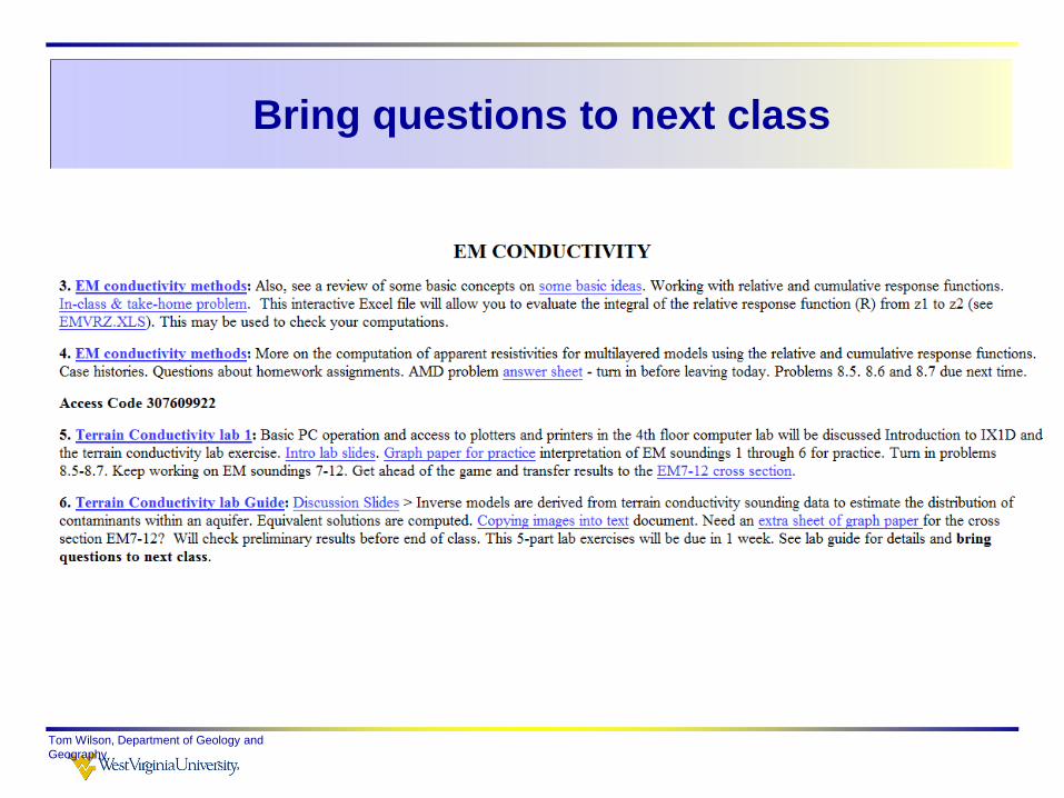
Overall learning objectives of the lab


• Develop terrain conductivity modeling skills

• Apply to specific subsurface problem: evaluate the hypothesis

that the aquifer down gradient from an industrial waste site may be

contaminated

• Constrain your models to be consistent with the local subsurface

geology: i.e., pay attention to the control well.

• Gain some familiarity with forward and inverse modeling

approaches.

• Answer some questions about the analysis you’ve undertaken

(see lab guide and last slide).

How did it go with cross section EM1-6


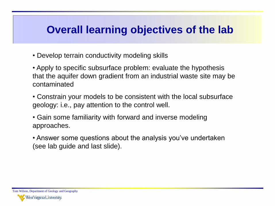
Address questions and move into the second

set of data EM7-12


Geography

Hopefully everyone has the text

We’re heading into chapter 5 on resistivity


Bring up IX1D while I go over a few ideas related to the

computer lab

Reminder of the problemsee page 19 terrain conductivity lab guide distributed today


Wastewater lagoon

Community down

gradient from the lagoon

Near surface clay layer

Aquifer

Thick silt layer underlies aquifer

1

2

3

contaminated,

uncontaminated?

Leaky?

Thicknesses do

not vary much

through the area

Resistivity

well

c

Hydraulic gradient

Review program displays

Questions about what you are seeing in this display?


31H34-10H

34-20H

34-40H

Appare

nt

Conductivity

“Effective” Penetration

Depth

“Conductivity of

individual layers

Depth

(m

)

The problems of an unconstrained inversion -

leave all variables un-fixed


We will assume that there is

some contamination and

introduce an upper

contaminated layer between

10 and 20 meters subsurface.

This first sounding is located at

a control well, so resistivities/

thicknesses are known. See lab

guide, page 19

Results of an unconstrained inversion


Doesn’t look much

like the local

geology inferred

from the resistivity

log data.


After multiple iterations – a near perfect fit (0.34% RMS error)

But – can we believe it? Is it even close?

Inverse models are always

non-unique. There exist

multiple solutions that can fit

the data with low error.

It’s hard to argue in favor of the results within

the context of the background geology


Geography

One should always retain a healthy

level of skepticism.

This result does not portray what we

know to be the case for this area.

Recall what we know from the control well and local geology.

We have to introduce constraints into the model



Aquifer


1

2

3

Control well

10m

20m

Uncontaminated reference

Get as much background geological and geophysical data

as possible before undertaking the modeling process.

In all the models developed in this lab exercise, you’ll

start with the same basic set of layers



Aquifer


1

contaminated

3

Control well

10m

20m

Uncontaminated reference

uncontaminated

Contaminated until proven otherwise

To consider the possibility of contamination, we need

to divide the aquifer into two layers


Near-surface clay layer

Aquifer

Thick silt layer

1

2

3

Control well

10m

20m

contaminated

4

contaminated

uncontaminated

Local wells indicate the aquifer has roughly constant

thickness of 20 m throughout the area, so we have to

incorporate this as a constraint in the final model.

Your starting model will always look like this

The conductivities of

the upper clay, fresh

water zone (if

present) and

underlying silt are all

known.

So we can fix those

parameters

The thickness of the

upper clay is also

known to be relatively

constant across the

area.

We fix that as well.



0.01% errorWe have information about

the subsurface geology that

we can use to constrain the

model: make it more

representative of the local

geology

Well location

EM1&7 are located at log wells & we’re pretty

sure what’s going on there

In both cases (1 and 7) we have an exact fit for

soundings at the borehole


No contamination. All

fresh water 10 mS/m

Underlying silt

Near

surface

layer

It’s the same for EM7

Comparison of unconstrained and constrained

model results – both have near zero error


In the end, our solutions are always non-unique.

22 meters

7 meters

Perhaps a little

contamination?

Fresh uncontaminated

water indicated by the log

from 10 to 30 meter depths


Key points about the local geology that help confine

the range of possible solutions

Local well data indicates that

•The near surface clay layer has nearly constant

thickness of 10 meters

•The aquifer also has relatively constant thickness

of 20 meters in the area. It is divided into two

zones: an upper contaminated zone and lower

uncontaminated zone.

•The conductivities of the near surface clay, the

fresh water leg in the aquifer and underlying silt

are 50 mS/m, 10mS/m and 15mS/m respectively.

Remember – you can use the

same starting model for each sounding


Within the context of the

well data, the geological

constraints allow us to fix

certain parameters during

the modeling processIn this way, we help push the

solution to one that is

geologically reasonable

Examine result and ask if it is consistent with

what we know about the area


Base of aquifer should

be here at 30 m

Questions about cross section construction?


We force the base of the aquifer to 30

meters. Remember – equivalent solutions

tell us this doesn’t change error much.

Develop models for EM7-12 but first let’s look at

equivalent solutions

I’ll work through EM3 you can pick one of EM8-12


Non-uniqueness

of solutions

Accept that results

are uncertain even

when constrained

and consider

equivalent solutions

Generate a model for one of the soundings EM8-12.

Honor constraints and see what you get.


You can make your

models fit the geology

Save your result

since you can use

it as part of the lab

assignment

Generate

equivalent models

Let’s go through the process of developing equivalent

solutions. Pick any sounding of EM8-12 you’d like


Geography

Look at the dashed lines

These are equivalent solutions


Geography

Note that equivalent

solutions (the dashed

lines) indicate that the

base of the aquifer can

be at 19 to 33 meters

subsurface.

We can use this to our

advantage and force

depth to the base of the

aquifer to 30 meters.

Why? We know enough

about the local geology

to place it around 30

meters

You can use the log scale to approximate value

between 10m and 20m and 20m and 30m etc.


16m17m19m

34m

Base of

contaminated zone

Base of aquifer

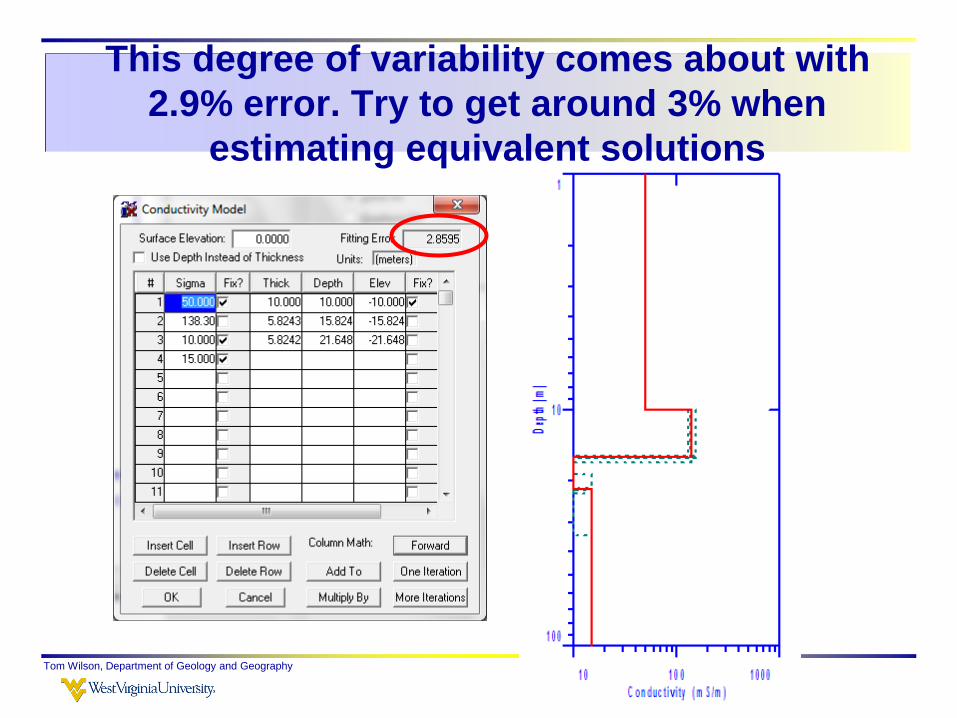
This degree of variability comes about with

2.9% error. Try to get around 3% when

estimating equivalent solutions


If the error is too low, you can move the layers

and conductivities around by clicking and

moving lines on the model


Pull values away from the initial inversion; do

one forward computation and one inversion;

then run equivalence


Tom Wilson, Department of Geology and Geography164.8

25.2

19.4121.35

Change these soundings to EM7 through EM12

Base of contaminated layer

Basal

Silt

The variability you get depends

on the amount of error you

leave in your model before

computing equivalent solutions

I’ll look over work and answer questions re

EM1-6, but for the remainder of the class get

started on EM7-12


Starting setupApparent

conductivities are

pretty high. Must

be contaminated.


EM7 EM8 EM9 EM10 EM11 EM12

Continue working through EM soundings 7 through 12

The lab is focused on these soundings

The formal lab requires that you analyze soundings EM7 through 12. Develop models of EM1-6 for practice and discussion today.

Depth to base of aquifer constrained by

local geologic mapping and well control in

the surrounding area?

Can you restrict aquifer

thickness to 20m?

How are contaminants

distributed across the

profile?

?

Let me check your work before leaving today

EM7 EM8 EM9 EM10 EM11 EM12

Practice sheet for EM soundings 7 through 12 – do as much as you can in class today

Depth to base of aquifer constrained by

local geologic mapping and well control

in the surrounding area?

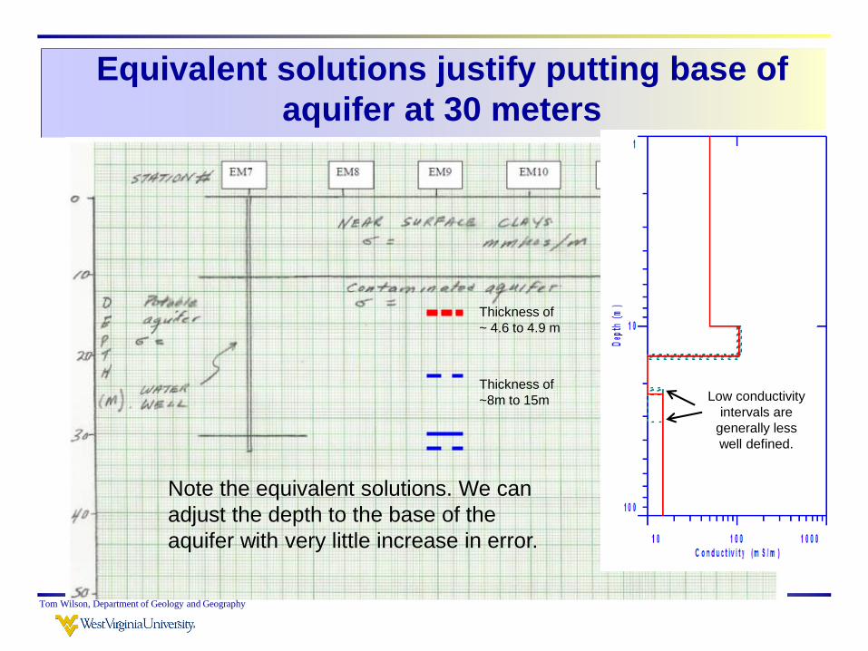
Equivalent solutions justify putting base of

aquifer at 30 meters


Thickness of

~ 4.6 to 4.9 m

Thickness of

~8m to 15m Low conductivity

intervals are

generally less

well defined.

Note the equivalent solutions. We can

adjust the depth to the base of the

aquifer with very little increase in error.


Get started on soundings EM7 through 12 and begin filling out the table below

Fill out as much of this table as you can and

let me check it off before leaving today

Name: ______________________

10

10

10

10

?

Activities


• Check off cross section EM1-6 – Questions?

• Check table EM7-12 before leaving.

• You should look over questions in lab guide (and on

next slide) Due date next Tuesday

•Writing Section should get Chapter summary outline

in this Thursday.

You should get most of this

completed for next time


Geography

Terrain Conductivity Lab (cont.)pages.geo.wvu.edu/~wilson/geol454/labs/TCLabDisc.pdf•Wrap up EM...

Documents

Transcript of Terrain Conductivity Lab (cont.)pages.geo.wvu.edu/~wilson/geol454/labs/TCLabDisc.pdf•Wrap up EM...