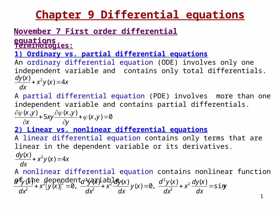
Terminologies:1) Ordinary vs. partial differential equationsAn ordinary differential equation (ODE) involves only one independent variable and contains only total differentials.

A partial differential equation (PDE) involves more than one independent variable and contains partial differentials.

2) Linear vs. nonlinear differential equationsA linear differential equation contains only terms that are linear in the dependent variable or its derivatives.

A nonlinear differential equation contains nonlinear function of the dependent variable.

1

November 7 First order differential equations

Chapter 9 Differential equations

xxyxdx

xdy4)(

)( 2

0),(),(

5),(

yxy

yxxy

x

yx

xxyxdx

xdy4)(

)( 2

ydx

xdyx

dx

xydxy

dx

xdyx

dx

xydxyx

dx

xydsin

)()( ,0)(

)()( ,0)(

)( 22

22

2

222

2

2

2

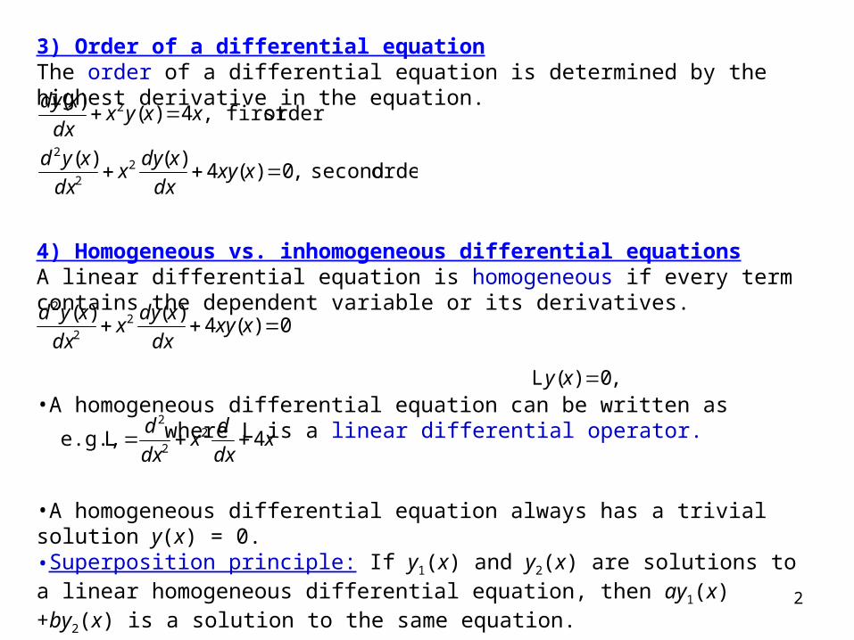
3) Order of a differential equationThe order of a differential equation is determined by the highest derivative in the equation.

4) Homogeneous vs. inhomogeneous differential equationsA linear differential equation is homogeneous if every term contains the dependent variable or its derivatives.

•A homogeneous differential equation can be written as where L is a linear differential operator.

•A homogeneous differential equation always has a trivial solution y(x) = 0.•Superposition principle: If y1(x) and y2(x) are solutions to a linear homogeneous differential equation, then ay1(x) +by2(x) is a solution to the same equation.

order second ,0)(4)()(

orderfirst ,4)()(

22

2

2

xxydx

xdyx

dx

xyd

xxyxdx

xdy

0)(4)()( 2

2

2

xxydx

xdyx

dx

xyd

,0)( xyL

xdx

dx

dx

d4 e.g., 2

2

2

L

3

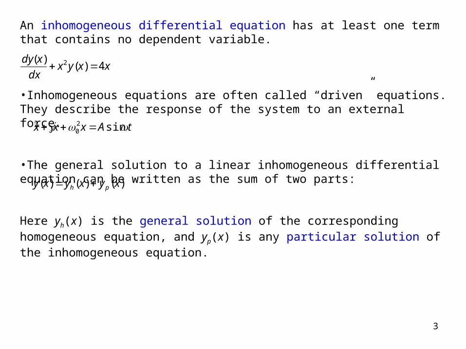
An inhomogeneous differential equation has at least one term that contains no dependent variable.

•Inhomogeneous equations are often called “driven” equations. They describe the response of the system to an external force.

•The general solution to a linear inhomogeneous differential equation can be written as the sum of two parts:

Here yh(x) is the general solution of the corresponding homogeneous equation, and yp(x) is any particular solution of the inhomogeneous equation.

xxyxdx

xdy4)(

)( 2

tAxxx sin20

)()()( xyxyxy ph

4

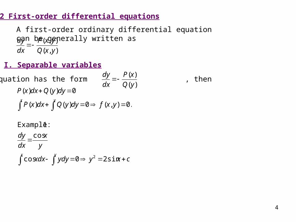
9.2 First-order differential equations

A first-order ordinary differential equation can be generally written as

)(

)(

yQ

xP

dx

dy

I. Separable variables

If the equation has the form , then

.0),(0)()(

0)()(

yxfdyyQdxxP

dyyQdxxPyx

),(

),(

yxQ

yxP

dx

dy

cxyydyxdx

y

x

dx

dy

yx

sin20cos

cos

:1 Example

2

5

m

tmgv

mg

m

tA

mgv

m

tA

mgv

ctmg

vm

dtmg

vdm

dtmg

v

mdv

dtmgv

mdv

mgvdt

dvm

expexp

exp

ln

ln

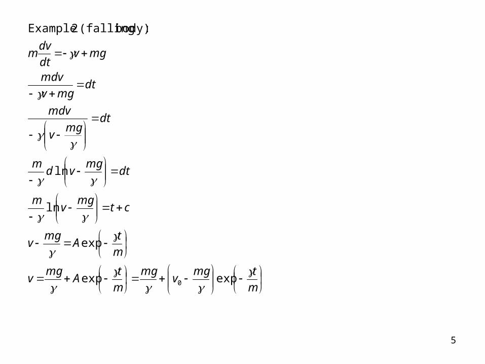
:body) (falling 2 Example

0

6

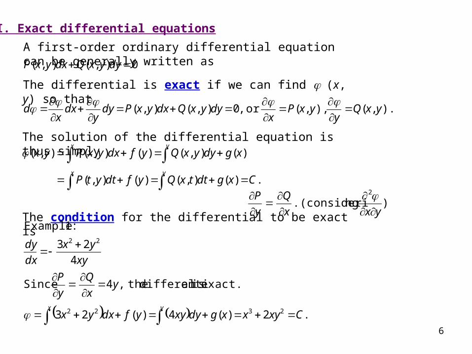
II. Exact differential equations

0),(),( dyyxQdxyxP

A first-order ordinary differential equation can be generally written as

The differential is exact if we can find (x, y) so that

).,( ),,(or ,0),(),( yxQy

yxPx

dyyxQdxyxPdyy

dxx

d

The solution of the differential equation is thus simply

The condition for the differential to be exact is

.)(),()(),(

)(),()(),(),(

yx

yx

CxgdttxQyfdtytP

xgdyyxQyfdxyxPyx

). ng(consideri . 2

yxx

Q

y

P

.2)(4)(23

exact. is aldifferenti the,4 Since

4

23

:1 Example

2322

22

Cxyxxgdyxyyfdxyx

yx

Q

y

P

xy

yx

dx

dy

yx

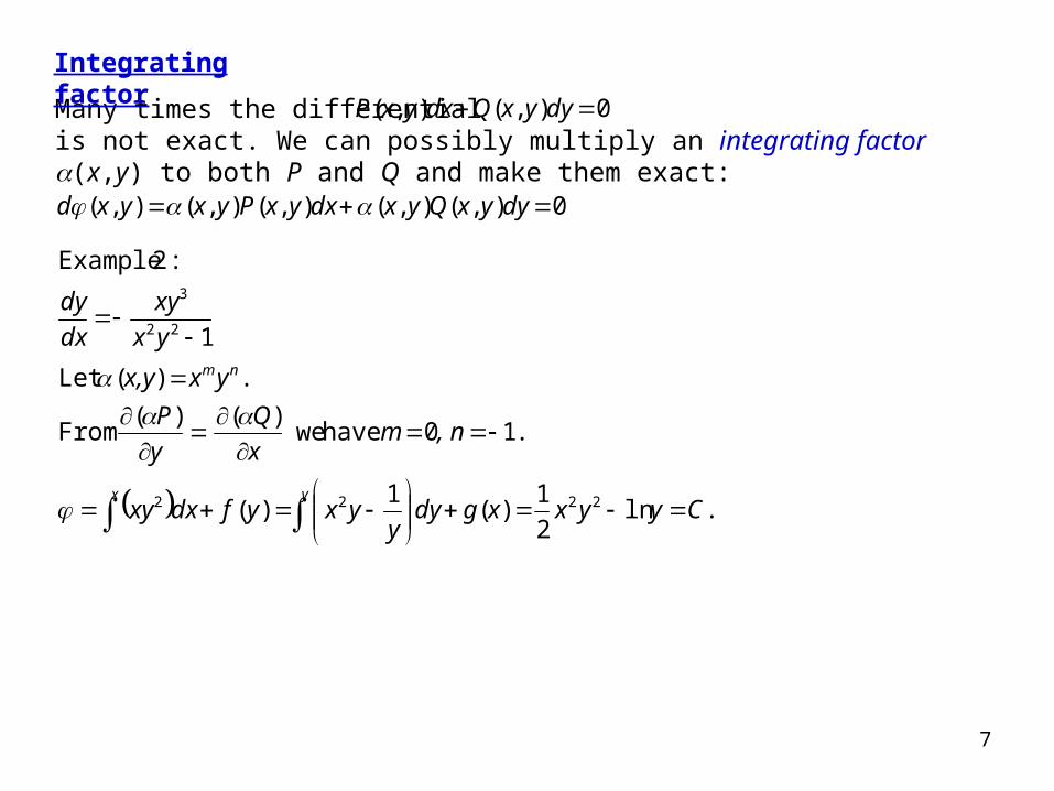
Many times the differential is not exact. We can possibly multiply an integrating factor (x,y) to both P and Q and make them exact:

7

Integrating factor

0),(),( dyyxQdxyxP

0),(),(),(),(),( dyyxQyxdxyxPyxyxd

.ln2

1)(

1)(

.10 have we)(

)(

From

.)(Let

1

:2 Example

2222

22

3

Cyyxxgdyy

yxyfdxxy

, nmx

Q

y

P

yxx,y

yx

xy

dx

dy

yx

nm

8

Read: Chapter 9: 1-2Homework: 9.2.2,9.2.3,9.2.4Due: November 18

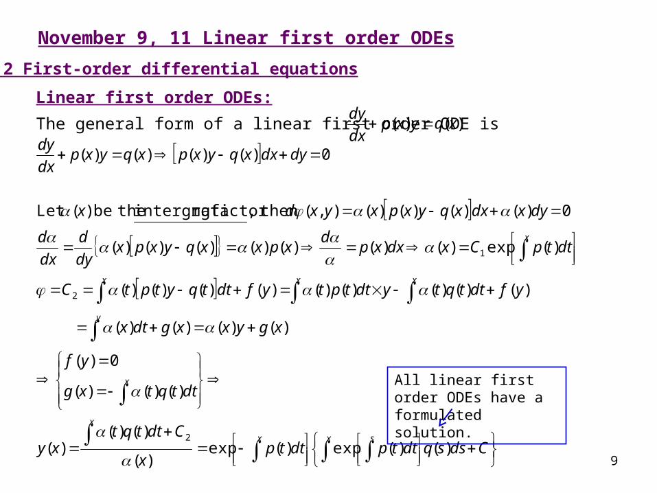
Linear first order ODEs:

The general form of a linear first order ODE is

9

November 9, 11 Linear first order ODEs

).()( xqyxpdx

dy

9.2 First-order differential equations

Cdssqdttpdttpx

Cdttqtxy

dttqtxg

yf

xgyxxgdtx

yfdttqtydttptyfdttqytptC

dttpCxdxxpd

xpxxqyxpxdy

d

dx

d

dyxdxxqyxpxyxdx

dydxxqyxpxqyxpdx

dy

x sx

x

x

y

x xx

x

)()(exp)(exp)(

)()()(

)()()(

0)(

)()()()(

)()()()()()()()()(

)(exp)()()()()()()(

0)()()()(),( then ,factor ngintergrati thebe )(Let

0)()()()(

2

2

1

All linear first order ODEs have a formulated solution.

10

2

322

2

2

23

5

1)(

.)ln2exp(2

exp)(

2 ,2

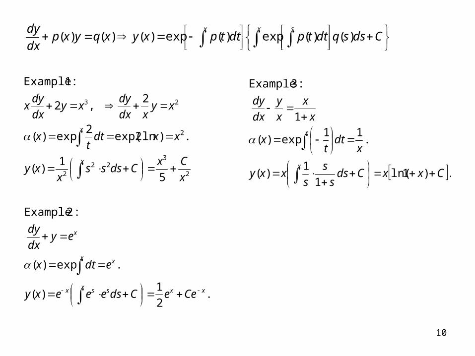
:1 Example

x

CxCdsss

xxy

xxdtt

x

xyxdx

dyxy

dx

dyx

x

x

.2

1)(

.exp)(

:2 Example

xxx ssx

xx

x

CeeCdseeexy

edtx

eydx

dy

.)1ln(1

1)(

.11

exp)(

1

:3 Example

CxxCdss

s

sxxy

xdt

tx

x

x

x

y

dx

dy

x

x

Cdssqdttpdttpxyxqyxp

dx

dy x sx)()(exp)(exp)()()(

11

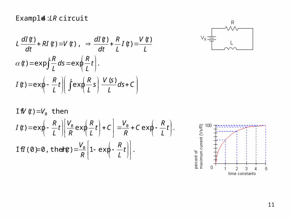
.exp1)( then 0,(0) If

.expexpexp)(

then)( If

)(expexp)(

.expexp)(

)()(

)( ),()(

)(

circuit :4 Example

0

00

0

tL

R

R

VtII

tL

RC

R

VCt

L

R

R

Vt

L

RtI

VtV

CdsL

sVs

L

Rt

L

RtI

tL

Rds

L

Rt

L

tVtI

L

R

dt

tdItVtRI

dt

tdIL

LR

t

t

12

)()( xqyxpdx

dy

)()()()(exp)(exp)(exp

)()(exp)(exp

xyxydssqdttpdttpdttpC

Cdssqdttpdttpy

ph

x sxx

x sx

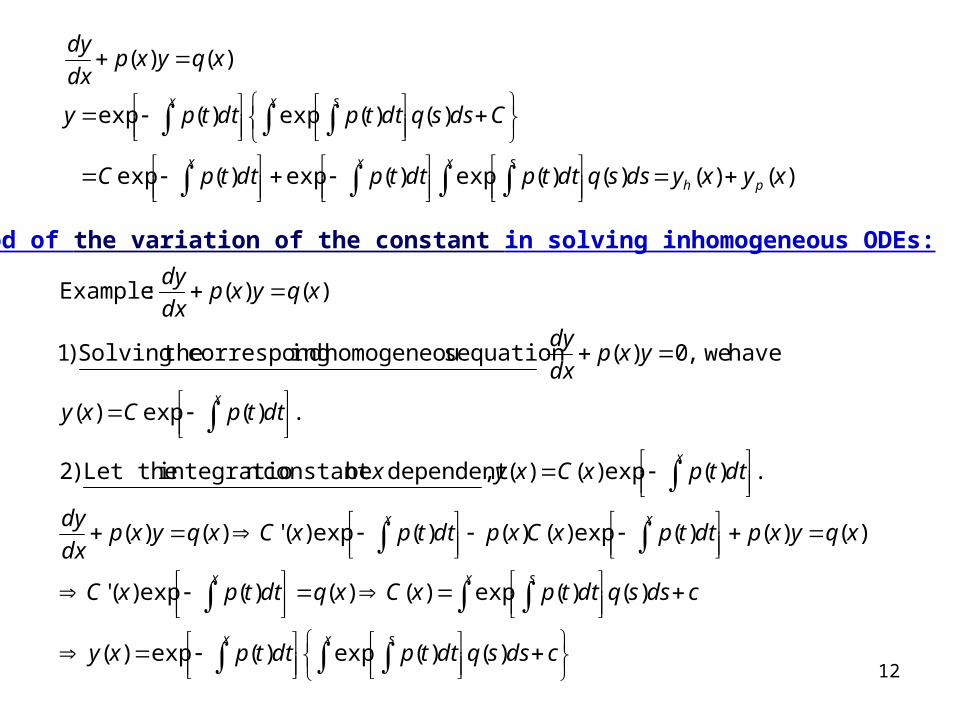
Method of the variation of the constant in solving inhomogeneous ODEs:

cdssqdttpdttpxy

cdssqdttpxCxqdttpxC

xqyxpdttpxCxpdttpxCxqyxpdx

dy

dttpxCxyx

dttpCxy

yxpdx

dy

xqyxpdx

dy

x sx

x sx

xx

x

x

)()(exp)(exp)(

)()(exp)()()(exp)('

)()()(exp)()()(exp)(')()(

.)(exp)()( ,dependent beconstant n integratio Let the )2

.)(exp)(

have we,0)( equation shomogeneou ingcorrespond theSolving )1

)()( :Example

13

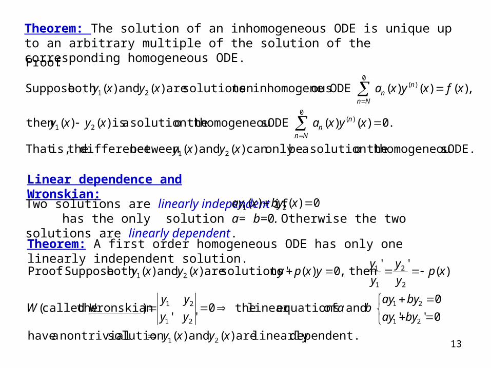
Theorem: The solution of an inhomogeneous ODE is unique up to an arbitrary multiple of the solution of the corresponding homogeneous ODE.

ODE. shomogeneou theosolution t a beonly can )( and )(between difference theis,That

.0)()( ODE shomogeneou theosolution t a is )()(then

,)()()( ODE ousinhomogenean tosolutions are )( and )(both Suppose

:Proof

21

0)(

21

0)(

21

xyxy

xyx axyxy

xfxyx axyxy

Nn

nn

Nn

nn

Linear dependence and Wronskian:

Two solutions are linearly independent if has the only solution a= b=0. Otherwise the two solutions are linearly dependent.

0)()( 21 xbyxay

Theorem: A first order homogeneous ODE has only one linearly independent solution.

dependent.linearly are )( and )(solution nontrivial a have

0''

0 and of equationslinear the0

'')Wronskian thecalled(

).(''

then ,0)(' tosolutions are )( and )(both Suppose :Proof

21

21

21

21

21

2

2

1

121

xyxy

byay

byayba

yy

yyW

xpy

y

y

yyxpyxyxy

14

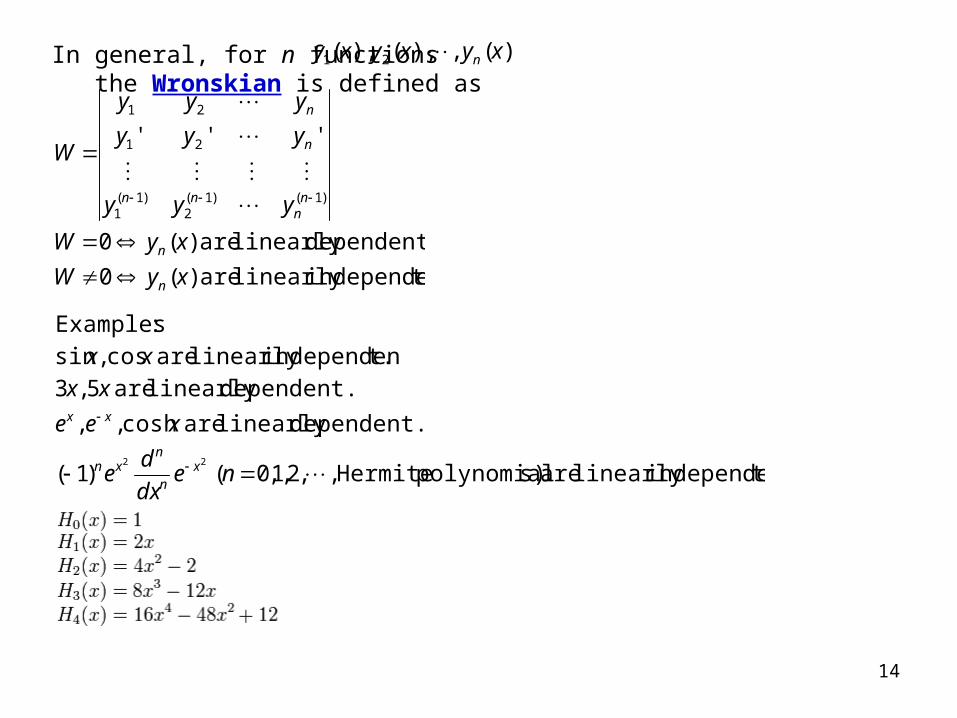
In general, for n functions the Wronskian is defined as ),( , ),( ),( 21 xyxyxy n

t.independenlinearly are )(0

dependent,linearly are )(0

'''

)1()1(2

)1(1

21

21

xyW

xyW

yyy

yyy

yyy

W

n

n

nn

nn

n

n

t.independenlinearly are s)polynomial Hermite,,2,1,0( )1(

dependent.linearly are cosh, ,

dependent.linearly are 5 ,3

t.independenlinearly are cos ,sin

:Examples

22

nedx

de

xee

xx

xx

xn

nxn

xx

15

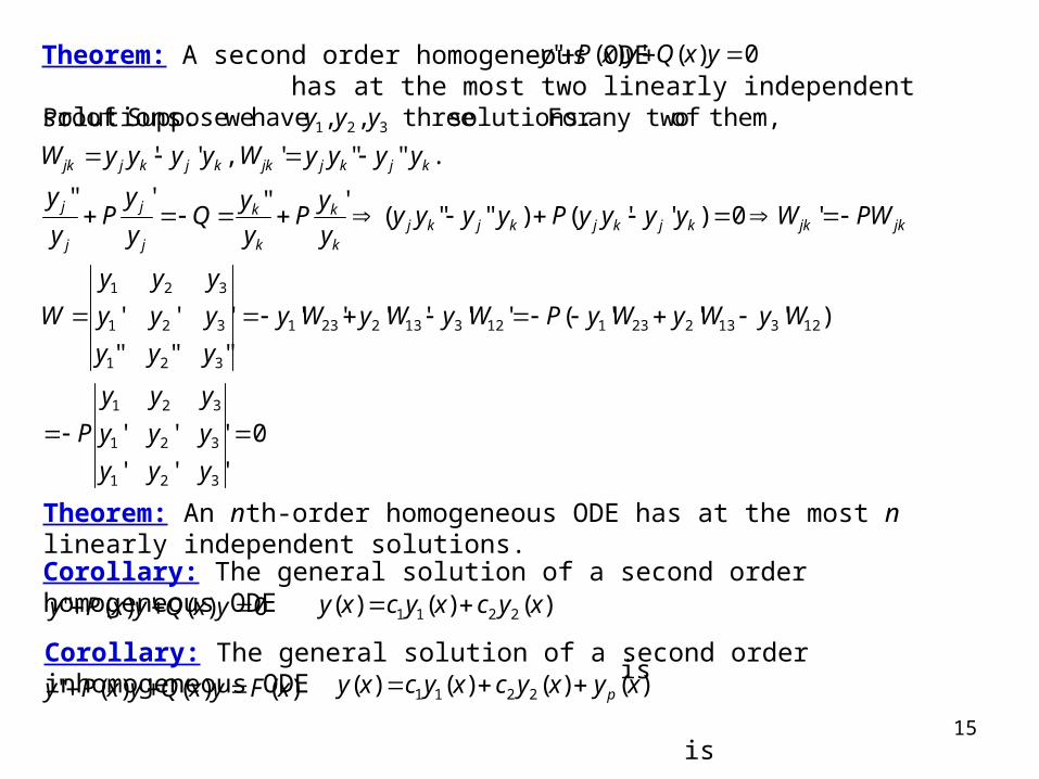
Theorem: A second order homogeneous ODE has at the most two linearly independent solutions.

0

'''

'''

)'''(''''''

"""

'''

'0)''()""('"'"

.""' ,''

them,of any twoFor solutions. three,, have weSuppose :Proof

321

321

321

123132231123132231

321

321

321

321

yyy

yyy

yyy

P

WyWyWyPWyWyWy

yyy

yyy

yyy

W

PWWyyyyPyyyyy

yP

y

yQ

y

yP

y

y

yyyyWyyyyW

yyy

jkjkkjkjkjkjk

k

k

k

j

j

j

j

kjkjjkkjkjjk

0)(')(" yxQyxPy

Corollary: The general solution of a second order homogeneous ODE is

).()()( 2211 xycxycxy 0)(')(" yxQyxPy

)()(')(" xFyxQyxPy Corollary: The general solution of a second order inhomogeneous ODE is

).()()()( 2211 xyxycxycxy p

Theorem: An nth-order homogeneous ODE has at the most n linearly independent solutions.

16

Read: Chapter 9: 2Homework: 9.2.11,9.2.13,9.2.14Due: November 18

17

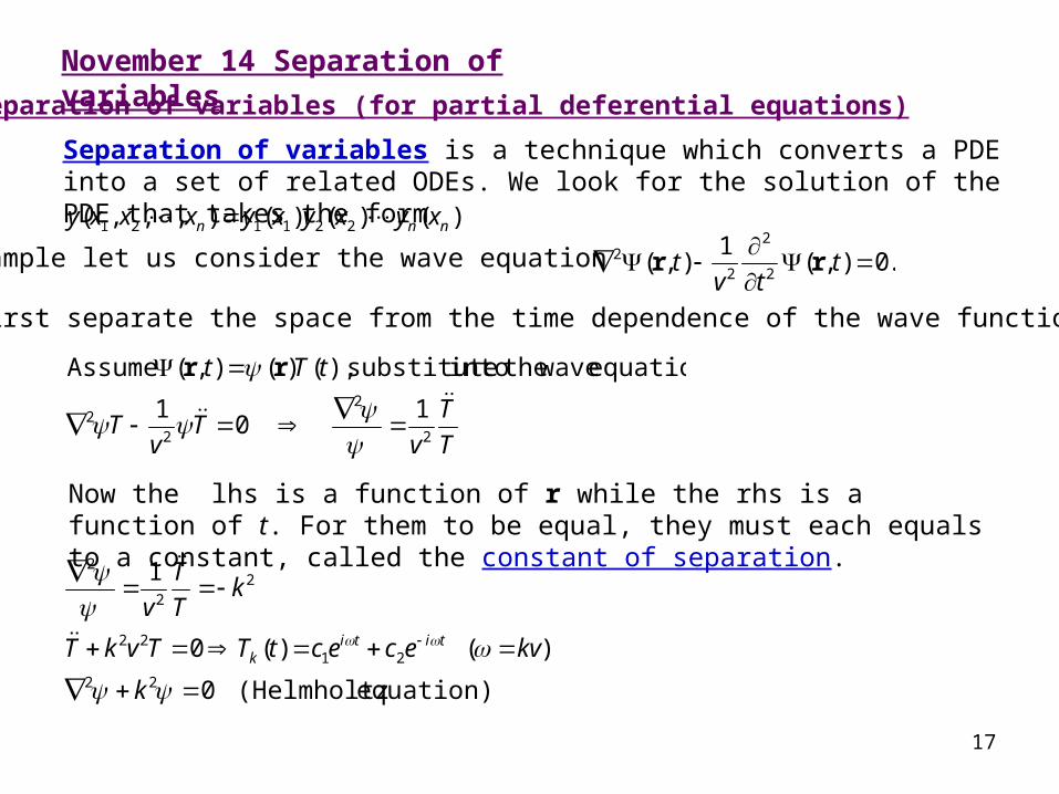
November 14 Separation of variables

9.3 Separation of variables (for partial deferential equations)

Separation of variables is a technique which converts a PDE into a set of related ODEs. We look for the solution of the PDE that takes the form

).()()( ),,,( 221121 nnn xyxyxyxxxy

As an example let us consider the wave equation

Let us first separate the space from the time dependence of the wave function.

.0),(1

),(2

2

22

ttv

t rr

T

T

vT

vT

tTt

2

2

22 1

01

equation, wave theinto substitute ),()(),( Assume

rr

Now the lhs is a function of r while the rhs is a function of t. For them to be equal, they must each equals to a constant, called the constant of separation.

equation) (Helmholtz 0

)( )(0

1

22

2122

22

2

k

kvecectTTvkT

kT

T

vtiti

k

18

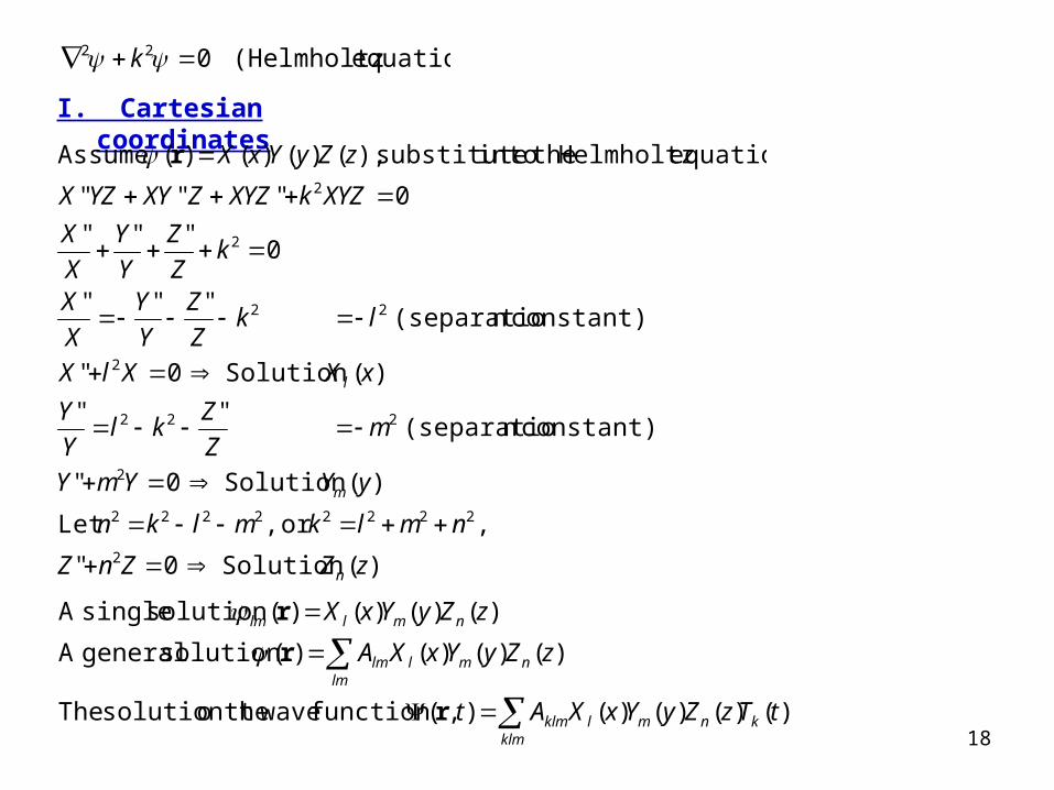
equation) (Helmholtz 022 k

I. Cartesian coordinates

)(Solution 0"

,or ,Let

)(Solution 0"

constant)n (separatio ""

)(Solution 0"

constant)n (separatio """

0"""

0"""

equation, Helmholtz theinto substitute ),()()()( Assume

2

22222222

2

222

2

22

2

2

zZZnZ

nmlkmlkn

yYYmY

mZ

Zkl

Y

Y

xXXlX

lkZ

Z

Y

Y

X

X

kZ

Z

Y

Y

X

X

XYZkXYZZXYYZX

zZyYxX

n

m

l

r

).()()()(),(function wave theosolution t The

)()()()(solution generalA

)()()()(solution singleA

tTzZyYxXAt

zZyYxXA

zZyYxX

kklm

nmlklm

lmnmllm

nmllm

r

r

r

19

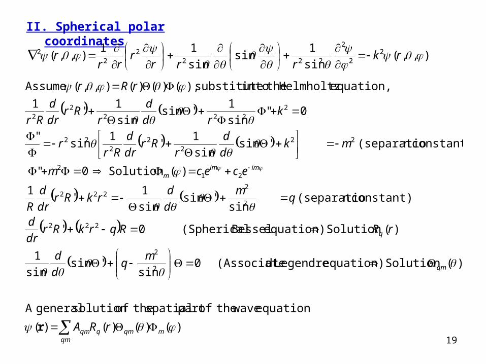
II. Spherical polar coordinates

),,(sin

1sin

sin

11),,( 2

2

2

2222

22

rk

rrrr

rrr

qmmqmqqm

qm

q

imimm

rRA

mq

d

d

rRRqrkRrdr

d

qm

d

drkRr

dr

d

R

ececm

mkd

d

rRr

dr

d

Rrr

krd

d

rRr

dr

d

Rr

rRr

)()()()(

equation wave theofpart spatial theofsolution generalA

)(Solution equation) Legendre d(Associate 0 sin

'sinsin

1

)(Solution equation) Bessel (Spherical 0'

constant)n (separatio sin

'sinsin

1'

1

)(Solution 0"

constant)n (separatio 'sinsin

1'

1sin

"

0"sin

1'sin

sin

1'

1

equation, Helmholtz theinto substitute ),()()(),,( Assume

2

2

222

2

2222

212

222

22

22

2222

22

r

20

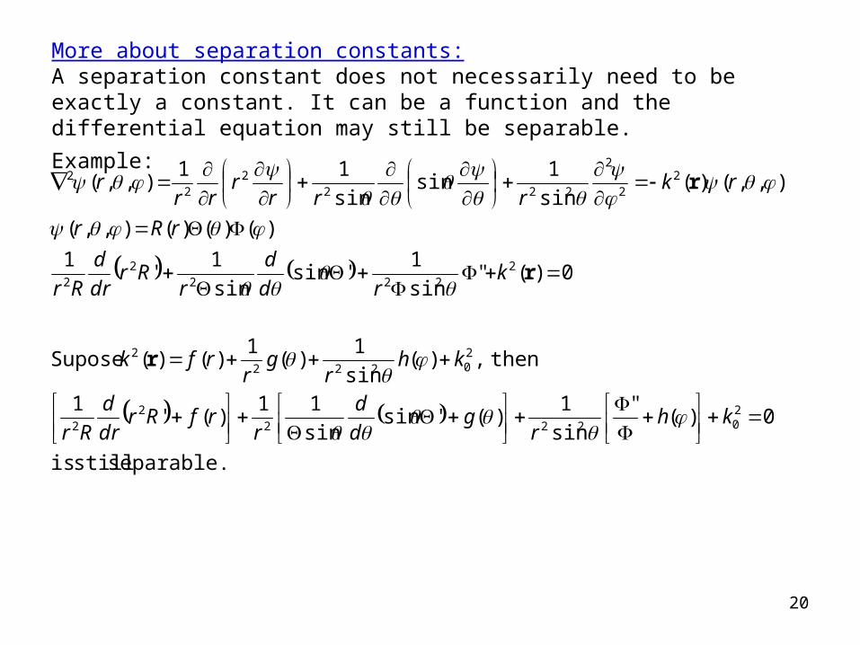
More about separation constants:A separation constant does not necessarily need to be exactly a constant. It can be a function and the differential equation may still be separable.

Example:

separable. still is

0)("

sin

1)('sin

sin

11)('

1

then,)(sin

1)(

1)()( Supose

0)("sin

1'sin

sin

1'

1

)()()(),,(

),,()(sin

1sin

sin

11),,(

20222

22

20222

2

2222

22

22

2

2222

22

khr

gd

d

rrfRr

dr

d

Rr

khr

gr

rfk

krd

d

rRr

dr

d

Rr

rRr

rkrrr

rrr

r

r

r

r

21

Read: Chapter 9: 3Homework: 9.3.4,9.3.9Due: December 2

22

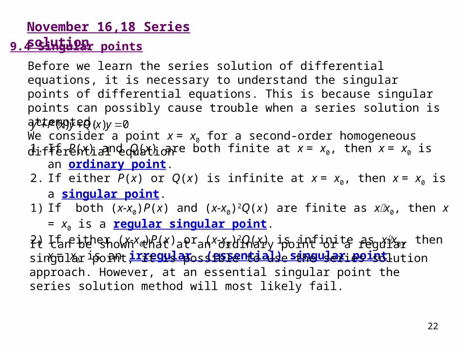
November 16,18 Series solution

9.4 Singular points

Before we learn the series solution of differential equations, it is necessary to understand the singular points of differential equations. This is because singular points can possibly cause trouble when a series solution is attempted.We consider a point x = x0 for a second-order homogeneous differential equation

0)(')(" yxQyxPy

1. If P(x) and Q(x) are both finite at x = x0, then x = x0 is an ordinary point. 2. If either P(x) or Q(x) is infinite at x = x0, then x = x0 is a singular point. 1) If both (x-x0)P(x) and (x-x0)2Q(x) are finite as xx0, then x = x0 is a regular singular

point. 2) If either (x-x0)P(x) or (x-x0)2Q(x) is infinite as xx0, then x = x0 is an irregular

(essential) singular point.

It can be shown that at an ordinary point or a regular singular point, it is possible to use the series solution approach. However, at an essential singular point the series solution method will most likely fail.

23

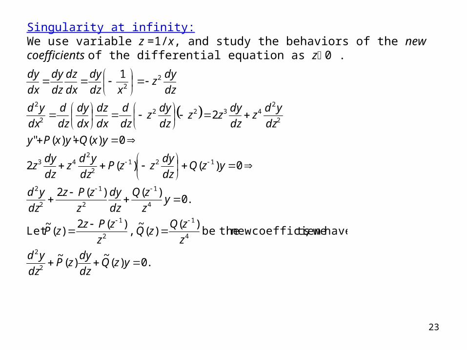
Singularity at infinity:We use variable z =1/x, and study the behaviors of the new coefficients of the differential equation as z 0 .

.0)(~

)(~

have we,tscoefficien new thebe )(

)(~

,)(2

)(~

Let

.0)()(2

0)()(2

0)(')("

2

1

2

2

4

1

2

1

4

1

2

1

2

2

1212

243

2

24322

2

2

22

yzQdz

dyzP

dz

yd

z

zQzQ

z

zPzzP

yz

zQ

dz

dy

z

zPz

dz

yd

yzQdz

dyzzP

dz

ydz

dz

dyz

yxQyxPy

dz

ydz

dz

dyzz

dz

dyz

dz

d

dx

dz

dx

dy

dz

d

dx

yd

dz

dyz

xdz

dy

dx

dz

dz

dy

dx

dy

24

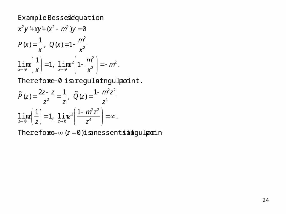
point.singular essentialan is 0)( Therefore

.1

lim ,11

lim

1)(

~ ,

12)(

~

point.singular regular a is 0 Therefore

.1lim ,11

lim

1)( ,1

)(

0)('"

equation sBessel' :Example

4

222

00

4

22

2

22

22

00

2

2

222

zx

z

zmz

zz

z

zmzQ

zz

zzzP

x

mx

mx

xx

x

mxQ

xxP

ymxxyyx

zz

xx

25

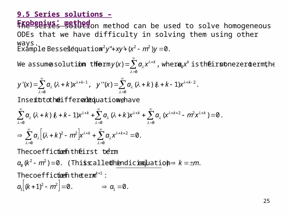
The series solution method can be used to solve homogeneous ODEs that we have difficulty in solving them using other ways.

9.5 Series solutions – Frobenius’ method

.0 .0)1(

: term theoft coefficien The

. .)equation indicial thecalled is (This .0)(

: first term theoft coefficien The

.0)(

0.)( )()1)((

have weequation, aldifferenti theintoInsert

.)1)(()('' ,)()('

then term,nonezerofirst theis where,)( form in thesolution a assume We

.0)('" equation sBessel' :Example

122

1

1

220

0

2

0

22

0 0

22

0

0

2

0

1

00

222

amka

x

mkmka

x

xaxmka

xmxaxkaxkka

xkkaxyxkaxy

xaxaxy

ymxxyyx

k

k

kk

kkkk

kk

kk

26

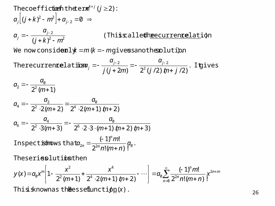
).(function Bessel theasknown is This

)!(!2

!)1(

)2)(1(22)1(21)(

thenissolution series The

.)!(!2

!)1( that shows Inspection

)3)(2)(1(322)3(32

)2)(1(22)2(22

)1(2

givesIt .)2/)(2/(2)2(

isrelation recurrence The

).solutionanother us gives ( only consider now We

.)relation recurrence thecalled is (This )(

0)(

:)2( term theoft coefficien The

0

2204

4

2

2

0

022

60

24

6

40

22

4

20

2

2

22

22

2

222

xJ

xnmn

ma

mm

x

m

xxaxy

anmn

ma

mmm

a

m

aa

mm

a

m

aa

m

aa

jmj

a

mjj

aa

mkmk

mkj

aa

amkja

jx

m

n

mnn

nm

n

n

n

jjj

jj

jj

jk

27

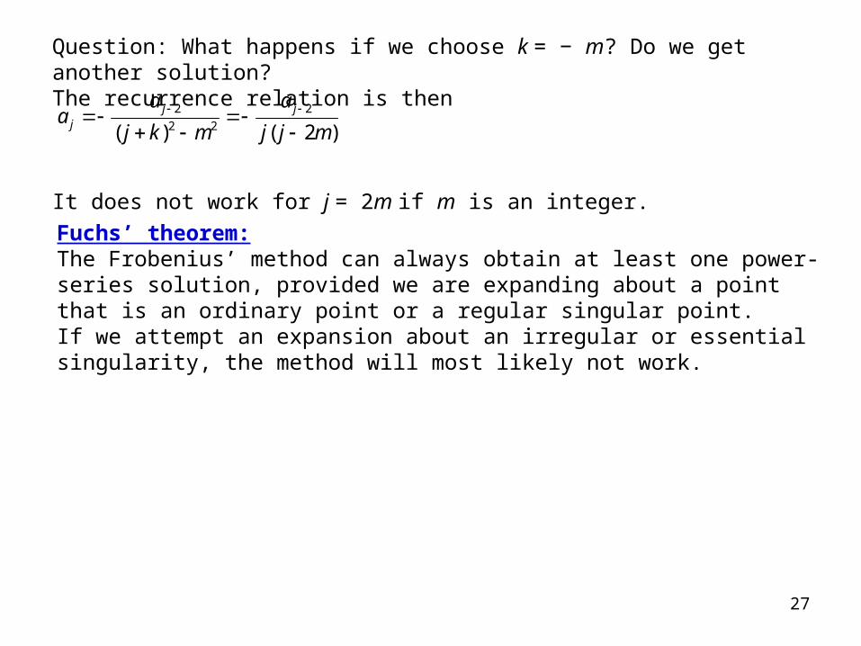
Question: What happens if we choose k = − m? Do we get another solution?The recurrence relation is then

It does not work for j = 2m if m is an integer.

)2()(2

22

2

mjj

a

mkj

aa jj

j

Fuchs’ theorem:The Frobenius’ method can always obtain at least one power-series solution, provided we are expanding about a point that is an ordinary point or a regular singular point.If we attempt an expansion about an irregular or essential singularity, the method will most likely not work.

28

Read: Chapter 9: 4-5Homework: 9.4.1,9.4.2,9.5.6(a),9.5.16Due: December 2

29

November 28 A second solution

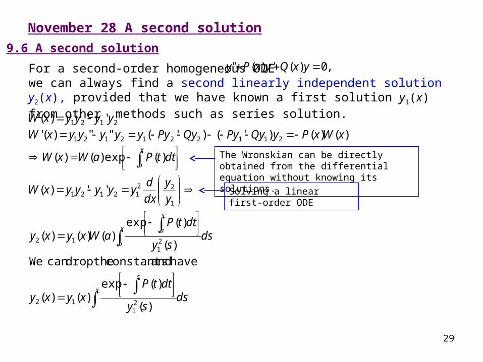
9.6 A second solution

For a second-order homogeneous ODE we can always find a second linearly independent solution y2(x), provided that we have known a first solution y1(x) from other methods such as series solution.

,0)(')(" yxQyxPy

dssy

dttPxyxy

dssy

dttPaWxyxy

y

y

dx

dyyyyyxW

dttPaWxW

xWxPyQyPyQyPyyyyyyxW

yyyyxW

x

s

x

b

s

a

x

a

)(

)(exp)()(

have and constants thedropcan We

)(

)(exp)()()(

'')(

)(exp)()(

)()()'()'("")('

'')(

21

12

21

12

1

2212121

2112212121

2121

The Wronskian can be directly obtained from the differential equation without knowing its solutions.

Solving a linear first-order ODE

30

.cossin

cossin

sin

1sin

)(

)(exp)()(

issolution secondA

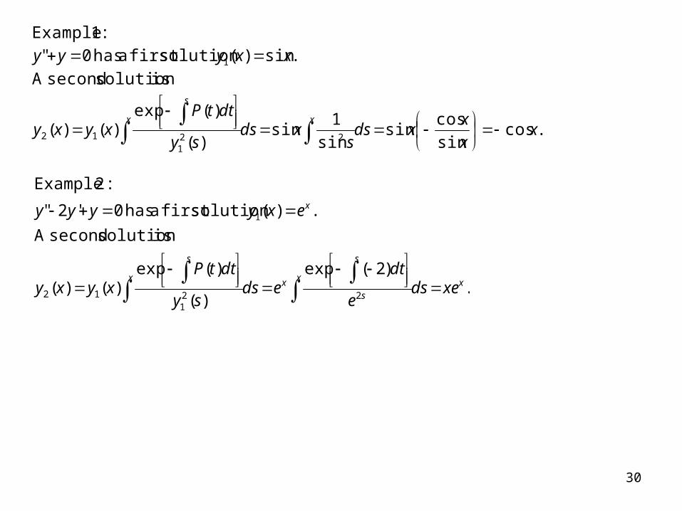
.sin)(solution first a has 0"

:1 Example

221

12

1

xx

xxds

sxds

sy

dttPxyxy

xxyyy

xx

s

.)2(exp

)(

)(exp)()(

issolution secondA

.)(solution first a has 0'2"

:2 Example

221

12

1

xx

s

s

xx

s

x

xedse

dteds

sy

dttPxyxy

exyyyy

31

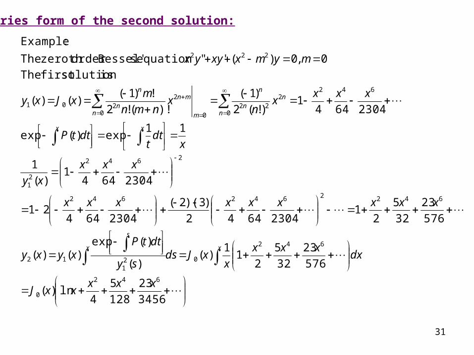
Series form of the second solution:

3456

23

128

5

4ln)(

576

23

32

5

21

1)(

)(

)(exp)()(

576

23

32

5

21

23046442

)3)(2(

230464421

23046441

)(

1

11exp)(exp

23046441

)!(2

)1(

)!(!2

!)1()()(

issolution first The

0 ,0)('" equation sBessel'order zeroth The

:Example

642

0

642

021

12

6422642642

2642

21

642

0

222

00

2201

222

xxxxxJ

dxxxx

xxJds

sy

dttPxyxy

xxxxxxxxx

xxx

xy

xdt

tdttP

xxxx

nx

nmn

mxJxy

mymxxyyx

xx

s

xx

n

nn

n

mn

mnn

n

32

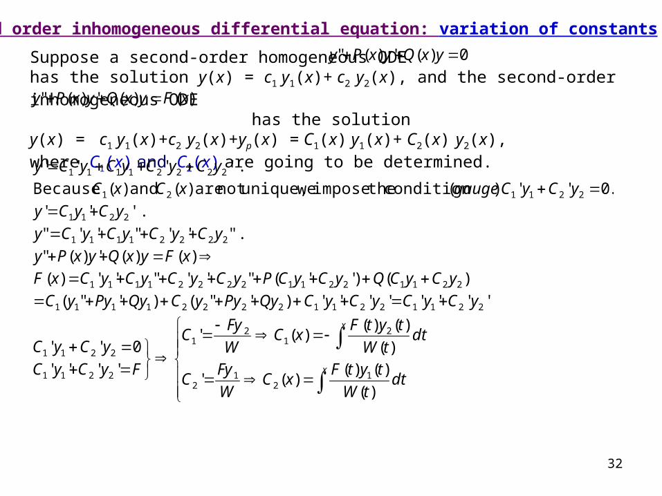
Second order inhomogeneous differential equation: variation of constants

Suppose a second-order homogeneous ODE has the solution y(x) = c1 y1(x)+ c2 y2(x), and the second-order inhomogeneous ODE

has the solutiony(x) = c1 y1(x)+c2 y2(x)+yp(x) = C1(x) y1(x)+ C2(x) y2(x),where C1(x) and C2(x) are going to be determined.

0)(')(" yxQyxPy

)()(')(" xFyxQyxPy

x

x

dttW

tytFxC

W

FyC

dttW

tytFxC

W

FyC

FyCyC

yCyC

yCyCyCyCQyPyyCQyPyyC

yCyCQyCyCPyCyCyCyCxF

xFyxQyxPy

yCyCyCyCy

yCyCy

yCyCgaugexCxC

yCyCyCyCy

)(

)()()('

)(

)()()('

''''

0''

'''''''')'"()'"(

)()''("''"'')(

)()(')("

".''"''"

'.''

.0'' )(condition theimpose weunique,not are )( and )( Because

'.''''

12

12

21

21

2211

2211

2211221122221111

2211221122221111

22221111

2211

221121

22221111

33

Read: Chapter 9: 6Homework: 9.6.6,9.6.9,9.6.15,9.6.19Due: December 9

34

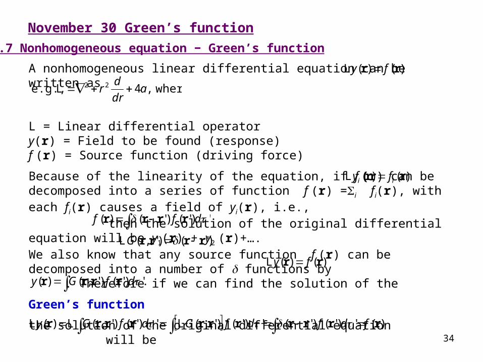
November 30 Green’s function

9.7 Nonhomogeneous equation − Green’s function

A nonhomogeneous linear differential equation can be written as

L = Linear differential operatory(r) = Field to be found (response)f (r) = Source function (driving force)

Because of the linearity of the equation, if f (r) can be decomposed into a series of function f (r) =i fi(r), with each fi(r) causes a field of yi(r), i.e., then the solution of the original differential equation will be y1(r) + y2 (r)+….We also know that any source function f (r) can be decomposed into a number of functions by . Therefore if we can find the solution of the

Green’s function

the solution of the original differential equation will be

Proof:

),()( rr fy L

where,4 e.g., 22 adr

dr L

')'()'()( dff rrrr

),'()',( rrrr GL

.')'()',()( dfGy rrrr

)()( rr fy L

).(')'()'(')'()',(')'()',()( rrrrrrrrrrr fdfdfGdfGy LLL

),()( rr ii fy L

35

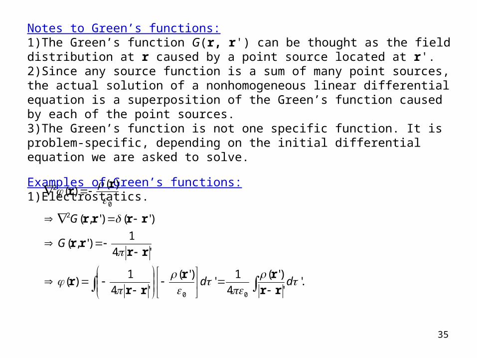
Notes to Green’s functions:1)The Green’s function G(r, r') can be thought as the field distribution at r caused by a point source located at r'.2)Since any source function is a sum of many point sources, the actual solution of a nonhomogeneous linear differential equation is a superposition of the Green’s function caused by each of the point sources.3)The Green’s function is not one specific function. It is problem-specific, depending on the initial differential equation we are asked to solve.

Examples of Green’s functions:1)Electrostatics.

.''

)'(

4

1'

)'(

'4

1)(

'4

1)',(

)'()',(

)()(

00

2

0

2

dd

G

G

rr

rr

rrr

rrrr

rrrr

rr

36

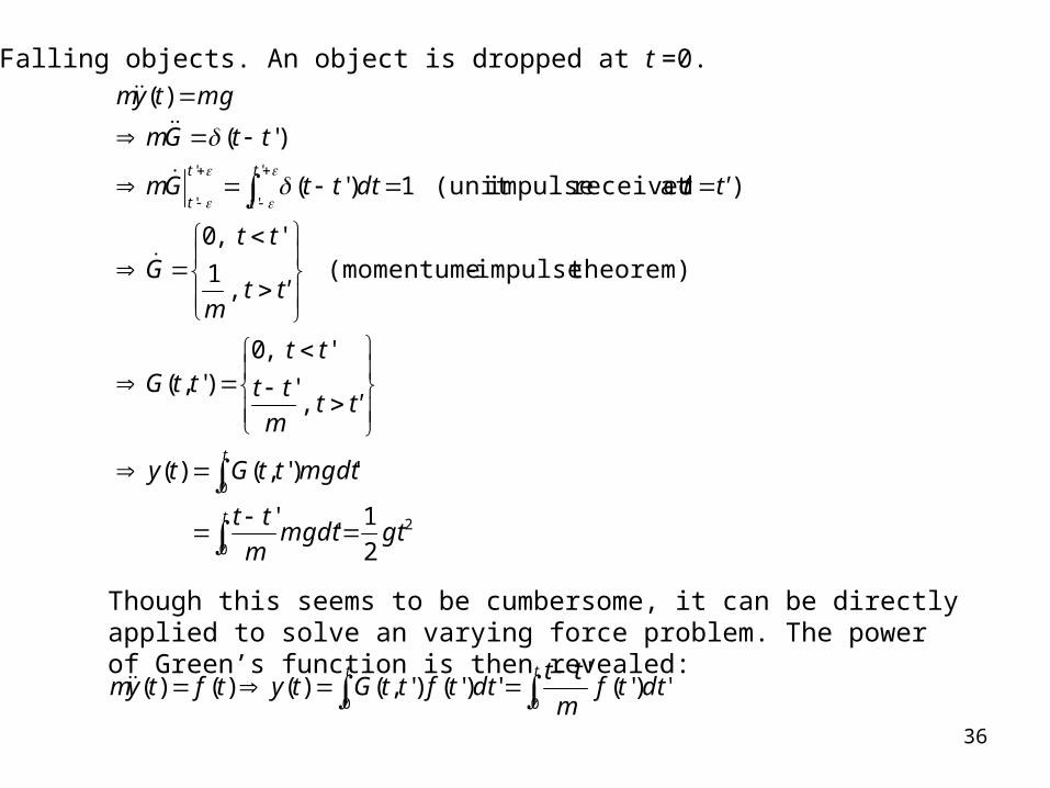
2) Falling objects. An object is dropped at t =0.

2

0

0

'

'

'

'

2

1'

'

')',()(

,'

' ,0)',(

theorem)impulse-(momentume ,

1

' ,0

)at received impulse(unit 1)'(

)'(

)(

gtmgdtm

tt

mgdtttGty

t'tm

tt

ttttG

t'tm

ttG

t'tdtttGm

ttGm

mgtym

t

t

t

t

t

t

Though this seems to be cumbersome, it can be directly applied to solve an varying force problem. The power of Green’s function is then revealed:

tt

dttfm

ttdttfttGtytftym

00')'(

'')'()',()()()(

37

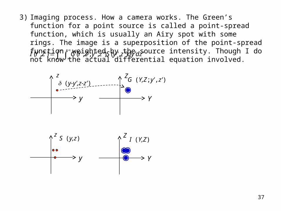
3) Imaging process. How a camera works. The Green’s function for a point source is called a point-spread function, which is usually an Airy spot with some rings. The image is a superposition of the point-spread function, weighted by the source intensity. Though I do not know the actual differential equation involved.

'')','()',';,(),( dzdyzySzyZYGZYI

y

(y-y',z-z')z

Y

G(Y,Z;y',z')Z

y

S(y,z)z

Y

I(Y,Z)Z

38

Read: Chapter 9: 7Homework: 9.7.5,6,15Due: December 9

39

Example of Green’s functions: Helmholtz equation.

k

ik

kk

k

k

k

k

k

k

k

i

dkk

e

kk

dG

dfkk

dd

kk

df

dA

kk

dfA

dfkkAdkkA

dfddkkA

dfddkkA

fdkkAfk

dA

dA

d

e,k

Gkfk

220

'

3220

*

220

*

220

*22

0

*'

'

*'

220'

220

*'

*'

220

*'

220

*'

220

20

2

21*

2/322

20

220

2

2

1)()'()',(

')'()()'(

)(')'()'(

)(

)()(

'

)()(

)()()'()'()(

)()()()()(

)()()()()(

)()()()()(

)()(

.)()( gives wavesplane by the )( expanding Suppose

).()()(set lorthonorma complete a forming

,2

1)( ionseigenfunct wave-palne thehave we)()(For

)'()',( )()( )(

21

rrkkk

kkk

k

kk

k

k

kkk

kkkk

kkkk

kk

kk

kk

kk

rkkkk

rrrr

rrr

rrr

r

rr

rr

rrkk

rrrr

rrrr

rrrr

rr

rrr

kkrr

rrr

rrrrrrrL

December 2 Helmholtz equation

40

k

ik

k

kk

k

k

k

i

dkk

e

kk

dG

dBG

kkB

ddkkBGk

dBG

dBGG

d

e,k

220

'

3220

*22

0

*

*220

20

2

*

2/322

2

1)()'()',(

)()',(

)'(

)()'()'()()()'()',(

)()',(

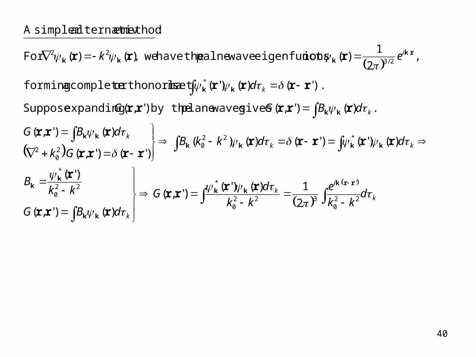
.)()',( gives wavesplane by the )',( expanding Suppose

).'()()'(set lorthonorma complete a forming

,2

1)( ionseigenfunct wave-palne thehave we)()(For

:method ealternativsimpler A

rrkkk

kk

kk

kkkk

kk

kk

kk

rkkkk

rrrr

rrr

r

rrrrrrrrr

rrr

rrrrr

rrrr

rrr

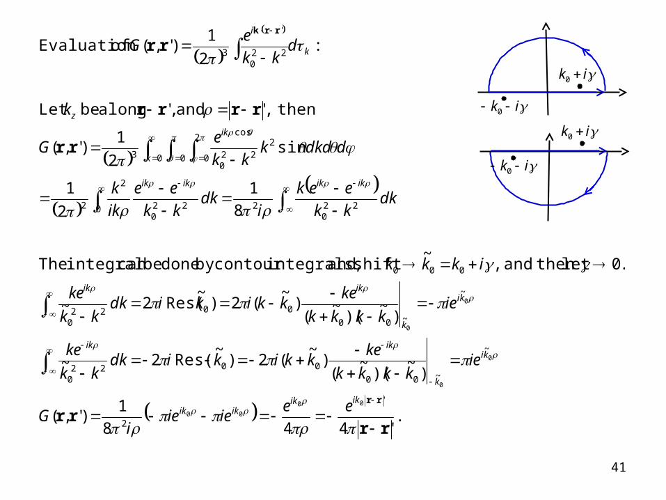
.'448

1)',(

)~

)(~

()

~(2)

~Res( 2~

)~

)(~

()

~(2)

~Res( 2~

.0let then and ,~

shift and integrals,contour by done becan integral The

8

1

2

1

sin2

1)',(

then,' and ,' along be Let

:2

1)',( of Evaluation

'

2

~

~00

00220

~

~00

00220

000

220

20 220

2

2

0 0

2

0

222

0

cos

3

220

'

3

00

00

0

0

0

0

rrrr

rr

rrrr

rr

rr

rrk

ikikikik

ki

k

ikik

ki

k

ikik

ikikikik

k

ik

z

k

i

eeieie

iG

iekkkk

kekkikidk

kk

ke

iekkkk

kekkikidk

kk

ke

ikkk

dkkk

eek

idk

kk

ee

ik

k

ddkdkkk

eG

k

dkk

eG

41

ik 0

ik 0

ik 0

ik 0

42

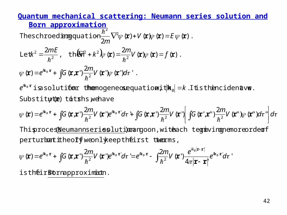
Quantum mechanical scattering: Neumann series solution and Born approximation

ion.approximatBorn first theis

''4

)'(2

')'(2

)',()(

terms,first two thekeeponly weIf on theory.perturbati

oforder more one giving each term with on, gocan )solution seriesNeumann ( process This

'")"()"(2

)",'()'(2

)',(')'(2

)',()(

have werhs, its to)( Substitute

ave.incident w theisIt . with equation, shomogeneou for thesolution a is

'.)'()'(2

)',()(

).()()(2

)( then ,2

Let

).()()()( 2

equation er schroeding The

''

2'

2

22'

2

0

2

222

22

22

0

0

000

00

0

0

dee

Vm

edeVm

Ge

ddVm

GVm

GdeVm

Ge

ke

dVm

Ge

fVm

kmE

k

EVm

iik

iii

ii

i

i

rkrr

rkrkrk

rkrk

rk

rk

rrrrrrr

rrrrrrrrrrr

r

k

rrrrr

rrrr

rrrr

43

Read: Chapter 9: 7No homework