Term structure estimation without using latent factors

Gregory R. Duffee∗

Haas School of BusinessUniversity of California – Berkeley

This Draft: January 2, 2005

ABSTRACT

A combination of observed and unobserved (latent) factors capture term structure dynam-ics. Information about these dynamics is extracted from observed factors using restrictionsimplied by no-arbitrage, without specifying or estimating any of the parameters associatedwith latent factors. Estimation is equivalent to fitting the moment conditions of a set ofregressions, where no-arbitrage imposes cross equation restrictions on the coefficients. Themethodology is applied to the dynamics of inflation and yields. Outside of the disinflation-ary period of 1979 through 1983, short-term rates move one for one with expected inflation,while bond risk premia are insensitive to inflation.

∗Voice 510-642-1435, fax 510-643-1420, email duffee@haas.berkeley.edu. Address correspondence to 545Student Services Building #1900, Berkeley, CA 94720. I thank Qiang Dai, George Pennacchi, RichardStanton, seminar participants at many universities, and discussants Francis Longstaff and Ken Singleton forhelpful comments. The most recent version of this paper is at http://faculty.haas.berkeley.edu/duffee/.

1 Introduction

Beginning with Vasicek (1977) and Cox, Ingersoll, and Ross (1985), researchers have built in-

creasingly sophisticated no-arbitrage models of the term structure. These models specify the

evolution of state variables under both the physical and equivalent martingale measures, and

thus completely describe the dynamic behavior of yields at all maturities. Much of this re-

search focuses on latent factor settings, in which the state variables are not directly observed

by the econometrician. Effectively, the evolution of yields is described in terms of yields

themselves. The important work of Piazzesi (2003) and Ang and Piazzesi (2003) broadens

this rather introspective view by including macroeconomic variables in the workhorse affine

framework of Duffie and Kan (1996). This extension allows us to investigate questions at

the boundaries of macroeconomics and finance. For example, what is the information in the

output gap about the compensation investors demand to face interest rate risk? What does

today’s inflation rate say about the components of expected future real returns to nominal

long-term bonds? Intensive research focuses on these and related questions using models

that describe the entire term structure with a combination of macroeconomic and latent

factors.1

Yet many of these questions can be examined without attempting to estimate the com-

plete dynamics of the term structure. In a general asset pricing setting, Hansen and Single-

ton (1982) show that restrictions implied by no-arbitrage can be exploited without using (or

knowing) the complete joint dynamics of asset prices and the pricing kernel. This idea is

easy to specialize to a term structure setting because a zero-coupon bond’s price is simply

the expected value of the pricing kernel at the bond’s maturity. By conditioning this ex-

pectation on a set of macroeconomic variables, combining it with the conditional dynamics

of the same variables, and adding a couple of assumptions about risk compensation, the

relation between bond prices and the macroeconomic variables can be determined without

specifying the remainder of the term structure.

This paper explains how to project the term structure onto a set of observed factors

and thereby extract information from the factors about the future evolution of the term

structure. I refer to this projection as partial term structure estimation. The remaining

variation in the term structure is driven by latent factors, but latent factors play no role in

either parameter estimation or in statistical tests of the model’s adequacy.

Partial term structure estimation offers two advantages to complete term structure es-

timation. First, estimation is simplified substantially because researchers avoid specifying

1Recent work includes Dewachter, Lyrio, and Maes (2002), Dewachter and Lyrio (2002), Hordahl, Tris-tiani, and Vestin (2002), Ang and Bekaert (2003), Ang, Piazzesi, and Wei (2003), and Rudebusch and Wu(2003).

1

features of term structure dynamics that are not of direct interest. Second, misspecification

is less likely to contaminate estimates of the dynamics that are of interest. For concrete-

ness, consider the relation between aggregate output and the term structure. We know that

output growth forecasts yields, while yields also forecast output growth. Capturing these

dynamics in a complete term structure model such as Ang, Piazzesi, and Wei (2003) requires

specifying the number of latent factors and functional forms for their dynamics. For exam-

ple, do latent factors follow moving average or autoregressive processes? Are such factors

Gaussian or do they exhibit stochastic volatility? Is the information in the latent factors

about future output primarily information about near term output growth (e.g., today’s one

quarter ahead forecast of output depends on today’s realization of shocks to latent factors)

or more distant output growth (e.g., today’s one quarter ahead forecast depends on lagged

shocks to latent factors)?

If our research goal is to model the complete term structure, we cannot avoid taking a

stand on its entire functional form. But if our goal is to use the information in the history of

output to forecast current and future bond yields and risk premia, latent factors are nuisance

features of the model. The estimation procedure proposed here puts little structure on these

factors. Neither the number of latent factors nor their functional relation with macro factors

are specified. Intuitively, the procedure can be viewed as the joint estimation of two sets

of regressions. The first set consists of regressions of changes in bond yields on changes in

the macro factors. These regressions are estimated with instrumental variables, where the

instruments are lagged macro factors. The second set are the regressions comprising a vector

autoregression for the macro factors. No-arbitrage imposes cross equation restrictions on the

parameters.

I use this estimation framework to study two questions concerning the relation between

inflation and the nominal term structure. First, how sensitive are short-term interest rates

to inflation? Second, how sensitive are bond risk premia to inflation? The empirical analysis

focuses on two periods. The first, from 1960 through the second quarter of 1979, is the “pre-

Volcker” sample. The second, from 1984 through 2003, is the “post-disinflation” sample. The

evidence indicates that during both periods, short-term rates move approximately one for

one with changes in expected future inflation, where the expectations are conditioned on the

history of inflation. This result might appear to contradict the existing Taylor rule literature

which concludes that the Fed reacted more aggressively to inflation in the disinflationary

period than it did in the pre-Volcker period. However, the discrepancy is largely driven by

the behavior of inflation and interest rates during 2002 and 2003.

Surprisingly, bond risk premia are fairly insensitive to inflation in both periods. Risk

premia are somewhat lower when inflation is high, but the contribution of inflation to vari-

2

ation in risk premia is economically small. The relation is strongest in the early period,

where the standard deviation of excess quarterly returns to a five-year bond conditioned

on inflation is about thirteen basis points. Put differently, the relation between changes in

inflation and changes in the shape of the term structure is determined almost entirely by

changes in expected future short rates, not by changes in risk premia.

The next section describes the modeling framework and the estimation methodology.

Section 3 applies the methodology to the relation between inflation and the term structure.

Section 4 concludes.

2 The model and estimation technique

Underlying the dynamics of bond yields is some structural model that explains these dynam-

ics in terms of the state of the macroeconomy, central bank policy, and investors’ willingness

to bear interest rate risk. Although the model here includes observable variables, it is not a

structural model. In particular, nothing here identifies monetary policy shocks. The model

is closer in spirit to a reduced form model linking bond yields to macro variables. The formal

structure is closely related to the model of Ang and Piazzesi (2003).

Time is indexed by discrete periods t. The length of a period is η years. There are n0

observable variables realized at time t and stacked in a vector f 0t . The natural application of

the model is to macroeconomic variables such as inflation and output. In principle, however,

this vector can include any observed variable that we are interested in relating to bond yields.

Accordingly, I generally refer to f 0t as a vector of observables rather than a vector of macro

variables.

The vector of observed factors ft used in the model contains lags zero through p − 1 of

f 0t :

ft ≡(f 0

t′f 0

t−1′. . . f 0

t−(p−1)′)′. (1)

The length of ft is nf = pn0. The choice of p is discussed at various places in this section.

For the moment, it is sufficient to note that lags are important both in forming forecasts

of future realizations of f 0t and in capturing variations in short-term interest rates that are

not associated with f 0t . In a term structure setting it is important to distinguish between

contemporaneous variables f 0t and the entire state vector ft. Bond prices depend on com-

pensation investors require to face one step ahead uncertainty in the state vector. In (1),

only f 0t is stochastic given investors’ information at t− 1.

The period t price of a bond that pays a dollar at period t+ τ is Pt,τ . The continuously

compounded annualized yield is yt,τ . The short-term interest rate, which is equivalent to the

3

yield on a one-period bond, is rt. Observed factors are related to the term structure, but

they are insufficient to explain the complete dynamics of the term structure. Latent factors

pick up all other variation in bond yields. There are nx latent factors stacked in a vector xt.

The relation between the factors and the short rate is affine:

rt = δ0 + δ′fft + δ′xxt. (2)

Bond prices satisfy the law of one price

Pt,τ = Et(Mt+1Pt+1,τ−1) (3)

where Mt+1 is the pricing kernel. The term structure of bond yields depends on the joint

dynamics of the pricing kernel, the observed factors, and the latent factors. To motivate the

method for estimating the relation between observed factors and the term structure, it is

easiest to start with the special case in which the observed factors are independent of the

latent factors. The estimation technique in the more general case of correlated factors only

requires a slight (but vital) modification to the method that is appropriate for independence.

2.1 Independence between observed and latent factors

The contemporaneous observed variables f 0t are assumed to follow a vector autoregressive

process (VAR) with at most p lags. We can always embed a VAR with fewer than p lags into

a VAR(p). Since the mathematics of affine term structure models are usually expressed in

terms of first order dynamics, it is convenient to express the observed dynamics as a VAR(1)

model for ft:

ft+1 − ft = µf −Kffft + Σfεf,t+1. (4)

The components on the right of (4) are

µf =

(µ0

0(nf−n0)×1

), Kff =

(K0

C

),

Σf =

(Σ0 0n0×(nf−n0)

0(nf−n0)×n0 0(nf−n0)×(nf−n0)

), εf,t+1 =

(ε0,t+1

0(nf−n0)×1

). (5)

The vector µ0 has length n0, the matrix K0 is n0 × nf , and the matrix Σ0 is n0 × n0. The

elements of the n0-length vector ε0,t+1 are independent standard normal innovations. The

4

companion matrix C has the form

C =

⎛⎜⎝

−I I 0 . . . 0 0

. . .

0 0 0 . . . −I I

⎞⎟⎠ . (6)

The square submatrices in C all have dimension n0. The double subscript on Kff is used

for consistency with the model of correlated factors presented in Section 2.3.

The dynamics of the latent factors have the general affine representation

xt+1 − xt = µx −Kxxxt + ΣxSxtεx,t+1, (7)

where Sxt is a diagonal matrix with elements

Sxt(ii) =√αxi + β′

xixt. (8)

The elements of εx,t+1 are independent standard normal innovations. No additional detail

about latent factor dynamics is either necessary or useful.

The pricing kernel has the standard log linear form

logMt+1 = −ηrt − Λ′ftεf,t+1 − Λ′

xtεx,t+1 − (1/2)(Λ′ftΛft + Λ′

xtΛxt). (9)

The vectors Λft and Λxt are the prices of εf,t+1 risk and εx,t+1 risk respectively. Since f 0t+1 is

the only component of ft+1 that is unknown at t, without loss of generality the former price

of risk can be expressed

Λft =

(Λ0t

0(nf−n0)×1

). (10)

The n0-vector Λ0t is the price of risk associated with innovations to f 0t+1. The price of

observed-factor risk, which is the product of observed-factor volatility and the compensation

for exposure to εf,t+1, depends on observed and latent factors:

ΣfΛft ≡(

Σ0Λ0t

0(nf−n0)×1

)=

⎛⎜⎝ λf + (λff λfx)

(ft

xt

)

0(nf−n0)×1

⎞⎟⎠ . (11)

The vector λf has length n0, the matrix λff is n0 × nf , and the matrix λfx is n0 × nx. This

is the Gaussian special case of the essentially affine price of risk introduced in Duffee (2002).

5

The price of risk associated with latent factor shocks has the similar form

ΣxSxtΛxt = λx + (λxf λxx)

(ft

xt

). (12)

Conditions under which this form satisfies no-arbitrage (in the continuous-time limit) are

discussed in Kimmel, Cheridito, and Filipovic (2004). As written, (12) allows the price of

latent factor risk to depend on both observed and latent factors. This general functional

form is tightened at the end of this subsection through the introduction of a key restriction.

The recursion used to solve for bond prices in an affine setting is standard. Campbell,

Lo, and MacKinlay (1997) provide a textbook treatment. I nonetheless go through a few of

the steps here for future reference. Guess that log bond prices are affine in the factors:

logPt,τ = Aτ +B′f,τft +B′

x,τxt. (13)

The recursion implied by law of one price (3), combined with the normally-distributed shocks

to ft and xt and independence between ft and xt, produces

Aτ +B′f,τft + B′

x,τxt = −ηrt + Aτ−1

+B′f,τ−1Et(ft+1) +B′

x,τ−1Et(xt+1)

+1

2

(B′

f,τ−1ΣfΣ′fB

′f,τ−1 +B′

x,τ−1ΣxS2xtΣ

′fB

′x,τ−1

)

−B′f,τ−1

⎛⎜⎝ λf + (λff λfx)

(ft

xt

)

0(nf−n0)×1

⎞⎟⎠

−B′x,τ−1

(λx + (λxf λxx)

(ft

xt

)). (14)

The factor loadings Bf,τ and Bx,τ are determined by this recursion. Substitute into (14)

the short rate equation (2) and the conditional expectation of ft+1 from (4), then match

coefficients in ft to determine one part of this recursion:

B′f,τ = −ηδ′f +B′

f,τ−1

(I −Kq

ff

)−B′x,τ−1λxf . (15)

The matrix Kqff in (15) is the counterpart to Kff under the equivalent martingale measure:

Kqff =

(K0 + λff

C

). (16)

6

Matching coefficients in xt produces another recursion that, combined with (15), allows for

the joint calculation of the loadings Bf,τ and Bx,τ . Yet another recursion produces the

constant terms Aτ . These other recursions are not relevant here.

The combination of the observed factor dynamics (4), the latent factor dynamics (7), and

the coefficients of log bond prices in (13) completely characterize the behavior of bond prices.

For example, both the unconditional expectation of logPt,τ and its expectation conditioned

on time t − 1 factor values can be calculated. This characterization allows estimation of

the model’s parameters using the dynamics of observed factors and bond yields. To date,

researchers using no-arbitrage models to study term structure dynamics have estimated these

complete term structure models. In other words, each parameter’s value is either fixed by the

researcher or estimated. The motivation behind this methodology is simple: our ultimate

goal is to understand all of the dynamic patterns in the term structure.

An alternative path to this goal requires less ambitious modeling efforts. Instead of

estimating all of the parameters of a term structure model that is unavoidably misspecified,

particular components can be estimated while leaving the remainder unspecified. This is the

point of the estimation procedure described in the next subsection. The relation between

observed factors and the term structure is estimated without characterizing the part of the

term structure that is unrelated to the observed factors. No parameters associated with

latent factors are estimated. In fact, not even the number of latent factors is specified.

An additional assumption is necessary. The price of risk of innovations in the latent

factors is assumed to not depend on the level of the observed factors. Formally, the general

form of the price of risk in (12) is restricted by

λxf = 0. (17)

The role of this assumption is highlighted in the next subsection.

2.2 Partial term structure estimation with independent factors

The parameters that are identified and estimated by this procedure are δf in (2), µ0 and K0

in (5), and λff in (11). There are three key results that guide the econometric methodology.

The first is that the observed factor loadings Bf,τ depend only on these parameters and not

on any parameters associated with the latent factors. With assumption (17), the loading

on the latent factors drops out of (15). We can solve explicitly the resulting recursion for

observed factor loadings without reference to the parameters of the latent factor dynamics:

Bf,τ = − (Kqff

′)−1 (I − (I −Kq

ff′)τ) ηδf . (18)

7

Given K0, λff , and the matrix of constants C defined in (6), the matrix Kqff is determined

by (16). Therefore the factor loadings in (18) can be computed.

The second key result is that the expectation of differenced log bond yields conditioned on

observed variables depends only on information about the observed variables. To understand

this result, first-difference the general bond-pricing equation (13), divide by the negative of

the bond’s maturity (in years) ητ to express it in terms of annualized yields instead of log

prices, and rearrange terms, denoting first differences with ∆:

∆yt,τ −(−B′

f,τ

ητ

)∆ft =

(−B′x,τ

ητ

)∆xt. (19)

The purpose of the first differencing is to remove both Aτ and the unconditional mean of the

latent factors. Next, remove any other information about the latent factors by taking the

expectation of (19) conditioned on ∆ft. Because ft and xt are independent, the conditional

expectation of the right side of (19) is zero:

E

(∆yt,τ −

(−B′f,τ

ητ

)∆ft

∣∣∣∣ ∆ft

)= 0. (20)

The conditional expectation depends only on Bf,τ and ∆ft.

The third key result is that conditional expectations of the observed factors identify the

physical dynamics of ft, and thus identify the parameters of these dynamics. From (4), the

expectation of ∆ft conditioned on ft−1 is:

E(∆ft|ft−1) − (µf −Kffft−1) = 0. (21)

The parameters that link the observed factors to bond yields can be estimated with Gen-

eralized Method of Moments (GMM) using the bond-pricing formula (18) and the moment

conditions (20) and (21). At each date t = 1, . . . , T we observe the contemporaneous ob-

served factors f 0t and the yields yt,τi

of L zero-coupon bonds with maturities τ1 through τL.

Denote a candidate parameter vector as

Φ =(µ0 δ′f vec(K0)

′ vec(λff )′)′. (22)

There are n0 + nf + 2n0nf parameters in Φ; n0 in µ0, nf in δf , and n0nf in each of K0 and

λff . Denote the true parameter vector by Φ0.

Given a parameter vector, the implied observed factor loadings Bf,τ1 through Bf,τLcan

8

be calculated with (18). The moment vector for observation t is

ht(Φ) =

⎛⎜⎜⎜⎜⎜⎜⎜⎜⎝

(∆yt,τ1 −

(−B′f,τ1

ητ1

)∆ft

)⊗ ∆ft

. . .(∆yt,τL

−(−B′

f,τL

ητL

)∆ft

)⊗ ∆ft

(∆f 0t − µ0 +K0ft−1) ⊗

(1

ft−1

)

⎞⎟⎟⎟⎟⎟⎟⎟⎟⎠. (23)

The unconditional expectation of ht is zero when it is evaluated at Φ0.

We can think of these moments as the moments associated with L + n0 ordinary least

squares (OLS) regressions, modified by the requirement of no-arbitrage. To make this clear,

consider the top expression in the moment vector, which represents nf moments associated

with the τ1-maturity bond. If no-arbitrage is not imposed, the vector Bf,τ1 is unrestricted.

Then this set of moments corresponds to the moments of the OLS regression of differenced

bond yields on differenced observed factors. (There is no constant term in the regression.)

Without the requirement of no-arbitrage, the estimate of −Bf,τ1/(ητ1) equals the coefficients

produced by this regression. Similar OLS regressions are estimated for each of the L bonds.

By imposing no-arbitrage, the coefficients from these regressions are required to satisfy cross

equation restrictions.

Now consider the bottom expression in the moment vector, which represents n0×(1+nf )

moments. If no-arbitrage is not imposed, it corresponds to the moments of n0 OLS regressions

of the VAR(p) model of the observed factors. The estimate of K0 is then determined by the

VAR parameter estimates. If no-arbitrage is imposed but the feedback matrix K0 under the

physical measure has no parameters in common with the feedback matrix K0 + λff under

the equivalent martingale measure, the interpretation of these moments is unchanged. If any

parameter restrictions are placed on λff , cross equation restrictions link the observed factor

dynamics and the bond price dynamics.

The parameter estimates solve

Φ∗ = argmaxΦ

gT (Φ)′WgT (Φ) (24)

where gT is the mean moment vector

gT (Φ) =T∑

t=1

ht(Φ) (25)

and W is some weighting matrix. The moment vector has length Lnf + n0(1 + nf ). If no

9

restrictions are placed on the model’s parameters, the number of moments less the number

of free parameters is nf (L− 1− n0). Thus all of the parameters are exactly identified when

the number of bonds L is one greater than the number of variables in the contemporaneous

observed vector f 0t . Including additional bonds produces overidentifying restrictions that

can be used to test the adequacy of the model.

2.3 Dependence between observed and latent factors

A large literature documents that the term structure contains information about future re-

alizations of some macro variables, such as output and inflation, that is not contained in

the history of these macro variables.2 Thus for at least some choices of observed variables,

the assumption of independence between observed and latent factors is untenable. This

subsection generalizes the model to allow for correlations between observed and latent fac-

tors. Conveniently, the partial term structure estimation technique described in Section 2.2

requires little modification in order to incorporate the correlation structure introduced here.

The following dependence is allowed between the observed and latent factors:

E(ft|xt−j) unrestricted, j > 0; (26)

E(xt|ft−j) = 0, j ≥ 0. (27)

Equation (26) allows the latent factors to forecast future observed factors, while (27) says

that observed factors have no forecasting power for current or future latent factors. This

second equation is less restrictive than it appears. In part, it imposes a normalization on

the decomposition of the short rate into pieces related to observable and latent factors.

A simple example helps illustrate the restrictions and normalizations built into (27). The

short rate is determined by contemporaneous inflation and the contemporaneous output gap:

rt = δ0 + πt + gt, (28)

where πt is inflation and gt is a measure of the output gap. (For simplicity, the coefficients

in this Taylor rule equation are both one.) The dynamics of output and inflation are:

gt = cg + θg,π,0πt + θg,π,1πt−1 + zt + εg,t; (29)

zt = θzzt−1 + εz,t; (30)

2The literature is too large (and only indirectly related to this paper) to cite fully. See Ang et al. (2003)and Diebold, Rudebusch, and Aruoba (2003) for discussions of this forecastability and references to therelevant literature.

10

πt = cπ + θππt−1 + ψεg,t−1 + επ,t. (31)

The shocks εg,t, εz,t, and επ,t are normally distributed and are independent at all leads and

lags. The coefficient θg,π,0 picks up any contemporaneous relation between shocks to inflation

and output. Inflation also leads output through θg,π,1. Output has a component zt that is

independent of inflation at all leads and lags, and a component εg,t that leads inflation.

An econometrician wants to investigate the relation between inflation and the term struc-

ture without using information about output. Thus from the econometrician’s perspective,

the short rate is driven by observed inflation and latent factors. There are a variety of ways

to express the short rate as the sum of observed and latent factors. One obvious expression

is simply (28) where ft = πt and xt = gt. But without information about output, it is impos-

sible to distinguish the direct link between inflation and the short rate from the indirect link

associated with the contemporaneous covariance between inflation and output. The natural

normalization is to impose a zero covariance between ft and xt, and it is imposed by (27)

with j = 0. With this normalization and the choice of ft = πt, xt is the residual from a

regression of gt on πt.

However, this decomposition does not satisfy all of the restrictions built into (27). When

ft = πt, there are two channels through which ft forecasts future short rates. First, current

inflation forecasts future inflation (and therefore future ft) through (31). Second, current

inflation forecasts the future output (and therefore future xt) through (29). The second

channel violates (27) for j > 0.

To satisfy (27), the vector of observed factors must be expanded to include lagged infla-

tion. The appropriate decomposition of rt into observed and latent factors is:

ft =

(πt

πt−1

), xt =

(zt

εg,t

), (32)

δf =

(1 + θg,π,0

θg,π,1

), δx =

(1

1

). (33)

With the definitions of ft and xt in (32), verification of (27) is straightforward. The second

element of xt is correlated with πt+j, j > 0, while xt is independent of πt−j, j ≥ 0.

The econometrician cannot rely on the structure of the model to produce this decompo-

sition, because by assumption no data on output are available to determine the dynamics in

(29). The appropriate rule to follow is that the vector ft must include all lags of πt that have

independent information about the short rate. Put somewhat differently, the choice of lag

length p maximizes the explanatory power of ft for the short rate. Since the econometrician

does not know the true data generating process of rt, a reasonable approach is to choose a

11

lag length and then test its adequacy by checking whether additional lags help to forecast

the short rate. Section 3.2 contains an application of this procedure.

Although ft requires only one additional lag of inflation in this example, alternative data

generating processes can require a large number of lags. To take an extreme example, replace

the dynamics of output and inflation above with the bivariate VAR

(πt

gt

)= θ

(πt−1

gt−1

)+ Σ

(ε1,t

ε2,t

)(34)

where the elements of θ and Σ are arbitrary. If gt is not observed, every lag πt−j contains some

independent information about the evolution of rt. Therefore unless ft contains an infinite

number of lags, (27) is technically violated. But in practice, the amount of independent

information in distant lags is too small to distinguish from sampling error.

The general model of correlated factor dynamics uses (7) for the dynamics of the latent

factors. These are the same dynamics used in the case of independence. The dynamics of

observed factors are:

ft+1 − ft = µf −Kffft −Kfxxt + Σfεf,t+1. (35)

Consider the “own” dynamics of observed factors: the dynamics conditioned only on the

history of the observed factors. From (35) and (27), these dynamics are

ft+1 − ft = µf −Kffft + ξt+1, (36)

ξt+1 = −Kfxxt + Σfεf,t+1, E(ξt+1|ft, . . . , ft−∞) = 0. (37)

In words, the own dynamics for ft are an AR(1) (with, perhaps, stochastic volatility intro-

duced by xt), or equivalently the own dynamics for f 0t are an AR(p).

The joint dynamics of the observed factors (35) and latent factors (7) must satisfy (27).

The fact that ft does not appear in (7) does not guarantee that (27) holds. The Appendix

describes parameter restrictions on Kfx and the latent-factor dynamics (7) that are sufficient

to imply (27). (The example at the beginning of this subsection is in the class of models

described in the Appendix.) Because Kfx and all of the components of (7) drop out of

the estimation procedure, these restrictions do not need to be imposed explicitly in the

estimation.

The model is completed with the dynamics of the pricing kernel in (9), which are the

same dynamics used for the case of independent factors. The functional forms for risk

compensation are (11) and (12), which also carry over from the case of independence.

12

Bond pricing formulas are calculated in the usual way. Guess the log-linear form (13)

holds and apply the law of one price. The result is (14). Although the form of this equation

is unchanged by the introduction of correlated factors, the interpretation is different. With

correlated factors, the period-t expectation of ft+1 depends on both observed and latent

factors. As in the case of independent factors, match coefficients from (14) in ft. This step

uses the special structure placed on the joint dynamics of ft and xt. Because Et(xt+1) does

not depend on ft, this matching results in the recursion (15), as in the case of independent

factors. Finally, by imposing assumption (17), the recursion for Bf,τ can be solved explicitly,

producing (18), as in the case of independence.

Why are the observed factor loadings Bf,τ unchanged when the assumption of indepen-

dence between observed and latent factors is dropped? The reason is the restrictions imposed

by (27). Because the latent factors are related to future observed factors but not to cur-

rent or past observed factors, the projection of the term structure onto observed factors is

unaffected by the latent factors. The projection throws away information in the term struc-

ture about the future evolution of the observed factors, but this information does not affect

the sensivity of yields to ft. Thus the only implication of introducing correlated factors is

that the model’s parameters can no longer be estimated with the technique described in

Section 2.2. The next subsection describes a modified technique.

Before discussing the estimation procedure, it is worth noting the consequences of using

a vector of observed factors ft that does not satisfy the conditional expectation requirement

(27). For concreteness, refer to the example presented at the beginning of this section.

Assume the econometrician uses ft = πt instead of ft = (πt πt−1)′. This choice of ft produces

a misspecified loading Bf,τ on πt. The problem arises in the matching of coefficients on ft

in (14). Because (27) is violated, the true conditional expectation Et(xt+1) depends on πt.

Therefore Bf,τ depends on Bx,τ−1, but this dependence is ignored in calculating Bf,τ . Hence

the econometrician is not only throwing away information in πt−1 that would help forecast

the term structure; the information in πt is also used incorrectly.

2.4 Partial term structure estimation with correlated factors

As in the case of independence, here the parameters δf , µ0, K0, and λff can be estimated

without imposing additional structure on the latent factors. There is one important differ-

ence. With independence, the expectation of the right side of (19) conditioned on ∆ft is

zero. With correlated factors, this is no longer true because xt−1 may contain information

13

about ft. Instead, take the expectation of (19) conditioned on ft−1 and apply (27):

E

(∆yt,τ −

−B′f,τ

ητ∆ft

∣∣∣∣ft−1

)= 0. (38)

The corresponding moment vector for observation t is

ht(Φ) =

⎛⎜⎜⎜⎜⎝

∆yt,τ1 −−B′

f,τ1

ητ∆ft

. . .

∆yt,τL− −B′

f,τL

ητ∆ft

∆f 0t − µ0 +K0ft−1

⎞⎟⎟⎟⎟⎠⊗

(1

ft−1

). (39)

Recall that with independence between observed and latent factors, the moment vector

(23) is interpreted as moments of OLS regressions where cross equation restrictions were

imposed on the OLS parameter estimates. Almost the same interpretation can be applied to

(39). The only difference is that the regressions of differenced yields on differenced observed

factors are estimated with instrumental variables instead of OLS. The instruments are a

constant and lagged observed factors. As with (23), no-arbitrage imposes cross equation

restrictions on the estimated parameters. Section 3 contains some additional discussion

about the inappropriateness of OLS moment conditions when the latent factors contain

information about future realizations of the observed factors.

This estimation procedure can use yields on bonds of any maturity. In particular, is

not necessary to observe the short rate. However, if the short rate is observed, a single

instrumental variable (IV) regression can be used to estimate the short rate loadings δf .

Denote the instruments used in the moment condition (39) as z′t−1 = {1 f ′t−1}. Write the

change in the short rate from t − 1 to t as the sum of two pieces: a component that is

projected on zt−1 and a residual. The result is

∆rt = δ′f (E(∆ft|zt−1)) +{δ′f (−Kfxxt + Σfεf,t) + δ′x∆xt

}(40)

where

E(∆ft|zt−1) = µf −Kffft−1. (41)

The residual term in curly brackets is orthogonal to ft−1. Thus a regression of changes in the

short rate on changes in the observed factors using instruments zt−1 produces a consistent

estimate of δf .

The remainder of this section examines in detail some of the features of this model. The

next subsection discusses the role played by the affine structure of the latent factors.

14

2.5 Relaxing the affine structure

The affine dynamics of the latent factors xt are not essential. The affine form guarantees

conditional joint log-normality of bond prices and the pricing kernel, which in turn pro-

duces the recursion (14) from the law of one price. This subsection describes an alternative

framework that allows nonlinear dynamics, where conditional joint log-normality is sim-

ply assumed. This framework leads to the identical estimation procedure described in the

previous subsection.

Replace the observed factor dynamics (35) with

ft+1 − ft = µf +Kffft +Kfx(xt) + Σfεf,t+1, (42)

where Kfx(xt) is an unspecified function of the latent factors that can be nonlinear. Replace

the latent factor dynamics (7) with

xt+1 − xt = Kxx(xt) + ΣxSx(xt)εx,t+1, (43)

where Kxx(xt) and Sx(xt) are also unspecified functions of the latent factors that can be

nonlinear. The innovations εf,t+1 and εx,t+1 are multivariate standard normal shocks that are

independent at all leads and lags. Therefore shocks to both types of factors are conditionally

normal. Independence between shocks to observed and latent factors is consistent with the

normalization that latent factors contain information about future realizations of observed

factors, but not information about current or past realizations. Both types of shocks appear

in the stochastic discount factor, which is the same function (9) used in the affine model.

Replace the affine form for log bond prices (13) with

logPt,τ = Aτ +B′f,τft + wτ (xt), (44)

where wτ (xt) is a (perhaps nonlinear) function of xt with conditionally normal shocks:

wτ (xt+1) = Et(wτ (xt+1)) + ετ,t+1, ετ,t+1 ∼ N (0,Vart(ετ,t+1)) . (45)

As with the shocks to the latent factors, the shocks to these functions of latent factors are

also independent of the shocks to observed factors εf,t+1. Equation (44) with τ = 1 replaces

the short rate equation (2).

The functional form of w(τ) is unspecified here, but it is not arbitrary. No-arbitrage

restricts the form of w(τ) given the form of w(τ − 1). Here I simply assume that there are

a sequence of functions w(1), w(2), . . . that satisfy no-arbitrage.

15

With these assumptions, the law of one price (3) implies

Aτ +B′f,τft + wτ (xt) = A1 +B′

f,1ft + w1(xt) + Aτ−1

+B′f,τ−1Et(ft+1) + Et(wτ−1(xt+1))

+1

2

(B′

f,τ−1ΣfΣ′fBf,τ−1 + Vart(ετ−1,t+1)

)−B′

f,τ−1ΣfΛft − Covt(ετ−1,t+1,Λ′xtεx,t+1). (46)

As with the affine model, the next step is to take the expectation of (46) conditioned on

ft. A few additional assumptions are necessary for the terms involving the latent factors to

drop out of this conditional expectation. The first two assumptions replace the restriction

(27). First, the component of the expectation of ft+1 that is related to the latent factors has

an expectation of zero when conditioned on ft:

E(Kfx(xt)|ft) = 0. (47)

Second, the expectation of w(τ) conditioned on both ft and ft−1 is zero for all τ :

E(w(τ)|ft, ft−1) = 0 ∀ τ. (48)

Third, the variance of ετ,t+1 conditioned on ft is constant:

E (Vart(ετ,t+1)|ft) = Vτ . (49)

Fourth, the conditional expectation of the compensation for facing observed-factor risk is

ΣfE (Λft|ft) =

(λf + λffft

0(nf−n0)×1

). (50)

Fifth, the restriction on the dynamics of latent-factor risk premia given in (17) is replaced

with

E (Covt(ετ−1,t+1,Λ′xtεx,t+1)|ft) = Cτ−1. (51)

The expectation of (46) conditioned on ft is therefore

B′f,τft = κτ +B′

f,1ft +B′f,τ−1(I −Kff − λff )ft (52)

where κτ is a maturity-dependent constant. Matching coefficients in ft produces the bond-

pricing formula (18) with ηδf = −Bf,1. The own dynamics of ft are a VAR(1). Thus the

16

model’s implications are identical to those of the affine model with correlated factors.

2.6 Applications

This subsection illustrates the kinds of questions that can be addressed with the partial term

structure estimation methodology.

• How does the expected time path of rt vary with ft?

The expected change in the short rate from t to t+ j, conditioned on ft, is

E(rt+j − rt|ft) = δ′f(I − (I −Kff )

j) (K−1

ff µf − ft

). (53)

Note that this j-ahead forecast is not a minimum-variance forecast. There is additional

information in the term structure (such as the current level of the short rate) that is ignored

in forming this conditional expectation. Therefore the partial term structure dynamics

should not be used to forecast, but rather to interpret the link between the observed factors

and the term structure.

• How do risk premia on bonds vary with ft?

The partial nature of the estimated model does not pin down mean excess bond returns.

However, it determines how variations in ft correspond to variations in expected excess

returns. The expected excess log return to a τ -maturity bond held from t to t+1, conditioned

on ft, is

E(logPt+1,τ−1 − logPt,τ − ηrt|ft) = κτ +B′f,τ−1

(λff

0(nf−n0)×nf

)ft. (54)

The constant term κτ is unrestricted.

• What is the shape of the term structure conditioned on ft?

The expectation of the τ -maturity annualized bond yield yt,τ , conditioned on ft, is

E(yt,τ |ft) = aτ +1

τδ′f(I − (I −Kq

ff

)τ) (Kq

ff

)−1ft. (55)

The constant term aτ is unrestricted.

• What is the expected evolution of the term structure conditioned on ft?

The j-period-ahead forecast of the change in the yield on a bond with constant maturity

17

τ is

E(yt+j,τ − yt,τ |ft) =

1

τδ′f(I − (I −Kq

ff

)τ) (Kq

ff

)−1 (I − (I −Kff )

j) (K−1

ff µf − ft

). (56)

• Is the empirical failure of the expectations hypothesis associated with ft?

Campbell and Shiller (1991) estimate regressions of the form

yt+s,l−s − yt,l = b0 + b1s

l − s(yt,l − yt,s) + et+s,l,s (57)

for maturities l > s. Under the weak form of the expectations hypothesis the coefficient

b1 should equal one, but in the data it is often negative. A common interpretation of this

result is that bond risk premia and the slope of the term structure are positively correlated.

The results of partial term structure estimation can be used to determine if the failure of

the expectations hypothesis is seen in the part of the term structure that is associated with

ft. Consider estimating (57) using ft as instruments. If the data are generated by the affine

model described in this section, the conditional expectation of yield spread on the right of

(57) is

E(yt,l − yt,s|ft) = θl,s +

(−1

lBf,l +

1

sBf,s

)′ft (58)

where θl,s is an unrestricted constant. The conditional expectation of the left side of (57) is

E(yt+s,l−s − yt,l|ft) = φl,s +s

l − sE(yt,l − yt,s|ft)

− 1

l − sB′

f,l−s

((I −Kff )

s − (I −Kqff

)s)ft (59)

where φl,s is an unrestricted constant. If λff = 0, then Kff = Kqff and the final term in (59)

is identically zero. In this case, the population estimate of b1 from IV estimation of (57) is

one. More generally, the population regression coefficient is

b1 = 1 − 1

s

[(−1

lBf,l +

1

sBf,s

)′Var(ft)

(−1

lBf,l +

1

sBf,s

)]−1

×(−1

lBf,l +

1

sBf,s

)′Var(ft)

((I −Kff )

s − (I −Kqff

)s)′Bf,l−s (60)

where Var(ft) is the unconditional variance-covariance matrix of ft. Given this variance and

the parameters of the term structure model, the regression coefficient can be computed.

18

The next section illustrates some of these applications by using the model to study the

joint dynamics of inflation and the term structure.

3 Inflation and the term structure

Researchers have long studied the relation between inflation and bond yields. This section

reexamines the relation using the model of correlated factors developed in Section 2.3. The

vector of observed factors consists of current and lagged inflation:

ft =(πt . . . πt−(p−1)

)′. (61)

The short rate equation (2) looks something like a Taylor (1993) rule regression. The Tay-

lor rule adds a measure of the period-t output gap to this equation and, depending on the

implementation, may include only contemporaneous inflation or impose constraints on the

parameters.3 The empirical analysis here uses information from the term structure to both

refine the estimate of the short rate’s loading on inflation δf and to simultaneously estimate

the sensitivity of the price of interest rate risk to the level of inflation. Ang and Piazzesi

(2003) investigate the latter issue using a different methodology. The next subsection de-

scribes the data sample.

3.1 The data

The data are quarterly from 1960 through 2003. The first date matches the beginning date

of Clarida, Galı, and Gertler (2000) in their empirical study of the Taylor rule. Inflation

in quarter t is measured by the change in the log of the personal consumption expenditure

(PCE) chained price index from t − 1 to t. Quarter-t bond yields are defined as yields

as of the end of last month in the quarter. This choice is a compromise between two

reasonable alternatives: using average yields within a quarter, as inflation is measured, or

using yields observed some time after the end of the quarter, to ensure the yields incorporate

the information in the announced inflation rate for the previous quarter. The short rate is

the three-month yield from the Center for Research in Security Prices (CRSP) risk free rate

file. Yields on zero-coupon bonds with maturities of one and five years are taken from the

CRSP Fama-Bliss file. Inflation and bond yields are continuously compounded and expressed

as annual rates.

3For example, the short rate in quarter t is often expressed as an affine function of inflation during thepast year, implying that ft contains lags zero through three of quarterly inflation and that δf(i) = δf(j), i �= j.

19

Table 1 reports summary statistics for various subperiods. Statistics are reported for

three subsamples separated by break points after 1979Q2 and after 1983Q4. The first break

point corresponds to the beginning of the Volcker tenure at the Fed and the accompanying

disinflation. There is substantial evidence that a regime change in the joint dynamics of

inflation and interest rates occurred at that time.4 Clarida et al. (2000) also use this break

point. The second break point corresponds to the end of the disinflation. Its precise place-

ment is somewhat arbitrary because it is harder to determine when the disinflation ended

than when it began. Using 1983Q4 allows for sufficient observations to identify the model’s

parameters during the disinflationary period.

Many characteristics of these data are common to all three periods, including the high

persistence of both inflation and yields. The estimation procedure assumes that both interest

rates and inflation are stationary processes. Although this assumption is typical in both the

term structure and Taylor rule literatures, it is motivated more by economic intuition and

econometric convenience than by statistical evidence. Unit root tests typically fail to reject

the hypothesis of nonstationarity for either interest rates or inflation. Contemporaneous

correlations between changes in inflation and changes in interest rates are fairly low, ranging

from about 0.25 in the early sample to about 0.10 in the late sample. Section 3.3 discusses

why these correlations understate the true relation between inflation and interest rates.

The focus on the three-month, one-year, and five-year yields is motivated by the following

considerations. The three-month maturity is the shortest consistent with the quarter-length

periods used in the model and the five-year maturity is the longest zero-coupon bond available

from CRSP. The one-year yield is at about the midpoint between these two years—not in

terms of maturity but in terms of comovement. Table 1 shows that in both the disinflationary

and post-disinflation periods, the correlation between quarterly changes in one-year yields

and three-month yields is within a percentage point of the corresponding correlation between

one-year yields and five-year yields. During the pre-Volcker period, variations in the one-year

yield are a little closer to variations in the long end of the term structure than the short end.

Yields on bonds of intermediate maturities are available, but including them has two con-

sequences. First, adding additional moment conditions expands the wedge between finite-

sample and asymptotic properties of GMM estimation. Second, using yields on bonds of

similar maturities increases the likelihood that the model’s parameter estimates will be de-

termined by economically unimportant properties of these yields. Efficient GMM estimation

emphasizes the linear combinations of yields that are statistically most informative about the

model. Moments involving yield spreads on similar-maturity bonds are likely to be highly

informative because such spreads exhibit little volatility. If the model is right and the yields

4See, e.g., Gray (1996) and the earlier research he cites.

20

are observed without noise, including bonds of similar maturities is a good way to pin down

the parameters. But the model is only an approximation to reality, and the zero-coupon

bond yields are interpolated. I therefore use a small number of points on the yield curve

that capture its general shape.5

Monthly observations of inflation and yields are also available. Monthly data contain

more information but their use requires both more parameters and more GMM moment

conditions. The number of inflation lags included in the vector ft must capture both the

autoregressive properties of inflation and the relation between lagged inflation and current

bond yields. These properties are driven more by calendar time than by frequency of obser-

vation. Thus shifting to monthly data will triple both the amount of available data and the

number of elements of ft. With n0 = 1 (a single contemporaneous observed variable) and

L bond yields, the number of moment conditions in (23) is p(L + 1) + 1 and the number

of moment conditions in (39) is (p + 1)(L + 1). The number of parameters is 1 + 3p. (The

AR(p) description of inflation uses 1 + p parameters and there are p parameters in both δf

and λff .) Hence the number of moment conditions and parameters increases almost propor-

tionally with p. Put differently, the number of data points per moment condition (and per

parameter) increases only slightly if monthly data are used. Quarterly data are used for the

sake of parsimony.

3.2 The choice of lag length

The number of elements p of ft must be at least as large as the number of lags necessary

to capture the autoregressive properties of inflation. To help choose this length, I estimate

autoregressions using up to six lags and calculate the Akaike and Bayesian Information

Criteria (AIC and BIC) for each. For the full sample, both criteria are minimized with three

lags. For the early sample, both criteria are minimized with a single lag. For the late sample,

the AIC is minimized with three lags and the BIC is minimized with a single lag. (None of

these results are reported in any table.)

Section 2.3 discussed the importance of including enough lags of inflation in ft to capture

all of the information in the history of inflation for the short rate. In other words, adding

additional lags to (61) should not increase the explanatory power of current and lagged

inflation. There is no consensus in the Taylor rule literature as to the proper lag length.

5A comparison with maximum likelihood term structure estimation may be helpful. One method usedto estimate an n-factor term structure model is to assume that n points on the term structure are observedwithout error and other points are contaminated by measurement error. In principle, any n maturities willwork, yet in practice the n maturities are widely spaced in order to force the model to fit the overall shapeof the term structure. The estimation procedure used in this paper does not rely on ad hoc noise, but as aconsequence it is more difficult to use information from many points on the term structure.

21

(That literature typically interprets lags in terms of slow reaction of the Fed to inflation and

output.) Using different econometric frameworks, Clarida et al. (2000), Rudebusch (2002),

and English, Nelson, and Sack (2003) arrive at different conclusions about the persistence of

the Fed’s reaction function. A recent review of the evidence is in Sack and Wieland (2000).

We might be tempted to rely on information criteria to choose the appropriate lag length

in the regression

rt = δ0 + δ′fft + ωt. (62)

But estimation of (62) is problematic for the same reason that estimation of the Taylor rule

is problematic: the residual exhibits very high serial correlation. To illustrate the problem,

consider estimation of (62) over the period 1984 through 2003. With three elements in ft,

the estimated equation is

rt = 1.82 + 0.53πt + 0.33πt−1 + 0.41πt−2 + ωt. (63)

The first-order autocorrelation of ωt is 0.9. This high autocorrelation makes it difficult to

test hypotheses and construct reliable standard errors. Accordingly, further discussion of the

choice of p is deferred in order to discuss in more detail methods to estimate the parameters

of (62). The choice of method critically depends on the relation between the residual ωt and

future inflation.

3.3 The relation between inflation and the short rate

Differencing is a natural method to correct for the high autocorrelation of ωt in (62):

rt − rt−1 = δ′f (ft − ft−1) + (ωt − ωt−1). (64)

The residual of (64) is much closer to white noise than is the residual of (62). If we adopt

the assumption that ωt−1 is orthogonal to ft, (64) can be estimated with OLS. However, this

assumption is inconsistent with both intuition and evidence.6 Investors at time t − 1 have

more information about inflation during t than is contained in the history of inflation. Since

investors care about real returns, presumably the short rate at t − 1 (which is a nominal

return earned during period t) depends on this information. If so, ωt−1 will be positively

correlated with ft. Therefore ft − ft−1 is negatively correlated with ωt − ωt−1 and the OLS

estimate of δf is biased. Similarly, contemporaneous correlations between changes in inflation

and changes in bond yields are relatively small because news about next period’s inflation

6A large empirical literature beginning with Fama (1975) considers the forecast power of interest ratesfor inflation.

22

rate dampens these correlations.

As discussed in the context of equation (40), estimation of (64) with a particular set of

instruments avoids this bias. The instruments are a constant and ft−1. Table 2 reports results

of estimating (64) with these instruments when ft contains lags zero to two of quarterly

inflation. Standard errors are adjusted for generalized heteroskedasticity and four lags of

moving average residuals using the technique of Newey and West (1987a).7 The results for

the full sample are puzzling. The sign of the estimated relation (negative) is wrong and

the standard errors are huge. Moreover, the fitted residuals are positively correlated with

contemporaneous changes in inflation. The intuition behind the bias in OLS coefficients

implies that this correlation should be negative.

By contrast, the subsample results are in line with our intuition, and contradict the

results from the full sample. In both the early and late periods, the coefficient on the

contemporaneous change in inflation is about 0.5. (This is also true in the disinflationary

period, but the disinflationary period results are shown only for completeness. There are too

few observations to draw any conclusions.) The coefficients on lagged changes in inflation

are also positive in both of these subperiods, while the correlations between fitted residuals

and contemporaneous changes in inflation are strongly negative. The negative correlation

implies that short rates lead inflation. Further evidence of this predictability is the positive

correlation between fitted residuals and the next quarter’s change in inflation. All of these

results are consistent with our intuition about the relation between inflation and interest

rates.

What explains the anomalous full-sample results? The assumptions underlying the IV

regression are not satisfied over the full sample because the relation between the instruments

and the explanatory variables has changed over time. In other words, inflation dynamics

over this period are not stable, as we can see from Table 3. In the early subperiod, inflation

basically follows an AR(1). In the late subperiod, inflation dynamics are more complicated.

The idea of the IV regression is that changes in short-term rates are projected on expected

changes in inflation, where expectations are conditioned on lagged inflation. For the purposes

of the regression, this expectation is proxied by an in-sample projection of changes in inflation

on lagged inflation. Because inflation dynamics have varied over the period, true conditional

expectations do not correspond to the full-sample projection. This problem is avoided by

splitting the sample into subperiods that exhibit stable dynamics.

The IV regressions help determine the proper lag length. Modify the regressions in Table

2 by adding a fourth lag of differenced inflation as both an explanatory variable and as

7The sample autocorrelations of the residuals (not reported in any table) are fairly close to zero at alllags.

23

an instrument. For all of these modified regressions, we cannot reject the hypothesis that

the coefficient on the additional lag of differenced inflation is zero. (These results are not

reported in any table.) Including lags zero through two of inflation in ft is therefore sufficient

to capture the dynamics of inflation in both the early and late subperiods.

3.4 Details of model estimation

To summarize, the relevant components of the term structure model are:

ft =(πt πt−1 πt−2

)′, (65)

rt − rt−1 = δ′f (ft − ft−1) + (ωt − ωt−1), (66)

E(πt|ft−1) − πt−1 = µ0 −K0ft−1 + ξt, (67)

Eq(πt|ft) − πt−1 = µq0 − (K0 + λff )ft−1 + ξq

t . (68)

The identified parameters are scalar µ0 and the vectors δf , K0, and λff , each of which has

three elements. Instead of reporting estimates ofK0, the tables report the implied coefficients

of the AR(3) for inflation,

ρ ≡(

1 0 0)−K0. (69)

The model allows the price of interest rate risk to depend on both contemporaneous

and lagged inflation. Results are reported only for the special case where the price of risk

depends on contemporaneous inflation, or λff(2) = λff(3) = 0. There are two reasons. First,

for both the pre-Volcker and post-disinflation periods, the more general functional form

does not provide any statistically significant improvement in fit. Second, estimation of the

general model over alternative subperiods sometimes produces an estimate of the equivalent-

martingale feedback matrix Kqff that fits the observed bond yields well, but implies wildly

implausible behavior for yields that are not included in the estimation.8

The model is estimated separately over the pre-Volcker period 1960Q1 through 1979Q2

and the post-disinflation period 1984Q1 through 2003Q4. For completeness, the model is also

estimated over the disinflationary period, although the sample period is too short to draw

any meaningful conclusions. In fact, for this 18 quarter period, the length of ft is set to two

because there are too few observations to estimate the model using the moments for three

elements. The GMM methodology is described in Section 2.4. The moment vector is (39).

Two iterations of GMM are performed. For the first iteration, the weighting matrix is the

8When this occurs, some eigenvalues of I − Kqff are typically imaginary with absolute values outside of

the unit circle.

24

inverse of the sample covariance matrix of the moments evaluated at “regression/constant

risk premia” parameters. These parameters are determined by an AR(3) regression of infla-

tion, IV estimation of (64), and λff = 0. The parameter estimates produced by this first

iteration are used to construct an asymptotically efficient weighting matrix and the param-

eters are estimated again. The covariance matrix of the moment vector is estimated using

the robust method of Newey and West (1987a) with four moving average lags. The solution

to the GMM optimization problem requires nonlinear optimization. To find the global min-

imum, 20 starting values are randomly generated. For each starting value, simplex is used

to determine a well-behaved neighborhood of the parameter estimates. A derivative-based

algorithm is used to improve the accuracy of the estimates.

3.5 Results

The results are displayed in Table 4. Panel A reports parameter estimates and Panel B

reports specification tests. The first specification test is the Hansen (1982) J test of overi-

dentifying restrictions. The second is a likelihood ratio test of the hypothesis δf = ρ. This

condition implies that short rates can be written as

rt = δ0 + E(πt+1|ft) + ωt. (70)

In other words, ex ante real short rates are uncorrelated with expected inflation. It has an

asymptotic χ2(p) distribution under the null. The third is a Lagrange multiplier test of the

hypothesis that the price of risk depends on the first two elements of ft instead of just the

first element. It has an asymptotic χ2(1) distribution under the null. The latter two test

statistics are derived in Newey and West (1987b).

There are three main conclusions to draw from these results. First, in both the early

and late periods there is a strong positive relation between the short rate and inflation. Of

course, we do not need a no-arbitrage model to tell us this; standard methods such as the

IV regressions in Table 2 also document this relation. The value of imposing no-arbitrage is

that the precision of the estimated relation is improved. The standard errors on δf in Table

4 are all smaller than the corresponding standard errors produced by the IV regressions.

Also note that in both periods, the magnitude of the estimated relation is stronger when

no-arbitrage is imposed than when it is not imposed. The features of the data contributing

to this pattern are discussed below.

The second conclusion is that short rates and expected inflation move almost one-for-

one. A comparison of the estimated δf vectors with the estimated AR(3) parameters reveals

they are almost identical in the early period. The correspondence is not quite as close

25

in the late period, but the hypothesis that δf = ρ cannot be rejected in either period.

This conclusion is surprising, since earlier research such as Clarida et al. (2000), Rudebusch

(2002), and Goto and Torous (2003) documented that short rates have been much more

sensitive to inflation rates in the post-deflationary period than prior to Volcker’s tenure.

These apparently conflicting results are resolved below.

The third conclusion is that there is a modest relation between inflation and bond risk

premia. The estimates of λff(1) are positive, implying that higher inflation corresponds to

lower bond risk premia.9 The estimate is statistically different from zero in the early sample

but not in the late sample. To get a sense of the magnitude of the reported coefficients,

consider the standard deviation of expected excess quarterly log returns to a five-year bond.

The standard deviation implied by the model can be computed with a combination of the

formula for expected excess returns (54) and the sample variance of the inflation state vector

ft. For the early sample, the implied standard deviation is 13.3 basis points, or 53 basis

points on an annual basis. For the late sample, the implied standard deviation is only 5

basis points on an annual basis.

What features of the data drive the high estimated sensitivity of the short rate and the

low sensitivity of risk premia? To explore this question, take a closer look at the behavior

of bond yields during 1984Q1 through 2003Q4. Table 5 reports estimates of the relation

between one-year and five-year bond yields and ft:

yt,τ = b0,τ + b′τft + et. (71)

The vector bτ is calculated with three alternative techniques. The first differences (71) and

estimates it with instrumental variables, paralleling the estimation of (64). The second uses

the IV estimate of (64) from Table 2, the AR(3) estimate of inflation from Table 3, and the

assumption that risk premia are invariant to ft. The vector bτ is then given by no-arbitrage

(ignoring the requirement that the computed vector for the one-year yield must be consistent

with the vector for the five-year yield). The third uses the parameter estimates of the no-

arbitrage model reported in Table 4 to compute bτ . No standard errors are reported in Table

5 because the only goal is to understand why the results of these three procedures differ from

each other.

Intuitively, estimation of the no-arbitrage model with GMM produces loadings of yields

on ft that are as close as possible to the IV estimates of these factor loadings, subject to

the requirement of no-arbitrage. A comparison of the first row of Table 5 with the second

reveals that the one-year yield is more sensitive to ft than is implied by the IV estimates of

9The log price loadings on inflation, Bf,τ , are negative (higher inflation implies lower prices). From (54),positive λff(1) implies a negative relation between expected excess log bond returns and inflation.

26

short-rate dynamics and constant risk premia. In fact, these IV estimates are larger than the

corresponding IV estimates for the short rate reported in Table 2. To fit the IV estimates

for the one-year yield, either the short rate needs to be more responsive to inflation or risk

premia need to be high when inflation is high.

If we attempt to reconcile the IV estimates for the short rate and the one-year yield simply

by adjusting the risk premia, no-arbitrage requires that the loadings for the five-year yield

exceed the loadings for the one-year yield. (In other words, inflation must be nonstationary

under the equivalent-martingale measure.) A comparison of the first and fourth rows of Table

5 reveals that this is counterfactual. Therefore GMM estimation picks short-rate loadings

δf that exceed the corresponding IV estimates, trading off fitting the short rate with fitting

the longer-maturity yields. The model-implied loadings for the one-year and five-year yields

(the table’s third and sixth rows) are fairly close to the IV-estimated loadings, although the

coefficients on contemporaneous inflation are too high and the coefficients on lagged inflation

are too low. These loadings are produced with a value of λff close to zero. If risk premia

increased when inflation increased (negative λff ), the loadings on inflation would be larger.

This would produce a better fit for the loadings on lagged inflation but a worse fit for the

loadings on contemporaneous inflation.

As mentioned above, much research documents the high sensitivity of interest rates to

inflation in the Volcker and Greenspan tenures. The results here do not support this result.

The reason is that more recent data are used here. Table 6 reports estimation results for the

post-deflationary period, with different ending points. The ending point of 1996Q4 matches

that in Clarida et al. (2000). Consistent with their evidence, the no-arbitrage results for

this sample implies a very high sensitivity of the short rate to inflation. The sum of the

coefficients on lags zero through two of the short rate exceeds two. Adding five years of data

(an ending point of 2001Q4) does not substantially affect these results. However, including

data for 2002 dramatically changes the results. With this sample, the estimated loadings on

inflation are economically small and statistically indistinguishable from zero.

Fig. 1 helps to explain these results. Panel A is constructed using the parameter estimates

from the no-arbitrage model estimated over the 1984Q1 through 2001Q4 period. It plots

one-quarter-ahead forecasts of changes in the five-year yield.10 The last two years are out-

of-sample forecasts in the sense that the model is estimated without these data, although

the forecast formed at quarter t−1 uses inflation data through quarter t−1. Panel B shows

the corresponding realization of the change in the five-year yield. (Note that the scales of

the two figures do not correspond; realizations are much more volatile than forecasts.)

10The predicted changes are consistently negative because the model is fitting the general fall in interestrates during the sample period.

27

Inflation was very low during early 2002. Therefore the AR model of inflation forecasted

rising inflation in late 2002, and correspondingly rising bond yields. In Panel A, two of the

largest predicted changes in the five year bond yield are the predictions formed in 2002Q1 and

2002Q2 for changes in 2002Q2 and 2002Q3, respectively. But bond yields fell substantially

during 2002. In, fact, the largest decline in the five-year yield during the entire sample period

occurs between 2002Q2 and 2002Q3. Thus the forecasts are spectacularly wrong in 2002.

The forecast accuracy improves in 2003, which is why estimation over the entire period finds

a statistically strong relation between inflation and bond yields.

3.6 Does the evidence support the model?

In both the pre-Volcker and post-disinflation periods, the formal tests of the overidentifying

restrictions do not come close to rejecting the model. Yet in a broader sense, these results

reinforce existing evidence that a single regime is an unsatisfactory description of the joint

dynamics of inflation and the term structure. Estimation of the model over the entire period

1960Q1 through 2003Q4 produces inflation factor loadings δf that are negative, much like

the IV estimates reported in Table 2 for the entire sample. (The full-sample results of the

no-arbitrage model are not reported in any table.) As previously discussed in the context of

these IV estimates, the problem with the full sample is that inflation dynamics have varied

substantially over time.

A more general no-arbitrage model needs to incorporate regime changes in inflation dy-

namics. Unfortunately, tractable bond pricing in a regime-switching framework requires a

number of restrictions on the nature of the regime switching; not all of the components of the

dynamics are allowed to switch regimes. The requirement of tractability leads to a variety

of nonnested regime-switching models. For example, the model of Ang and Bekaert (2003)

cannot accomodate changing factor dynamics, while the model of Dai, Singleton, and Yang

(2003) allows for changing dynamics only by imposing tight restrictions on the dynamics of

the price of interest rate risk.11 The results here suggest that a relatively simple regime-

switching framework can accurately fit these data. There is no need to allow for regime

changes in the compensation investors require to face inflation risk. In addition, the short

rate’s sensitivity to one-step-ahead forecasted inflation can be constant across regimes. The

only component that must shift regimes is the AR process followed by inflation. Whether

these simple dynamics are consistent with a tractable bond-pricing framework is an open

question.

11Ang and Bekaert (2003) discuss the modeling advantages and disadvantages of regime-switching factordynamics.

28

4 Concluding comments

This paper makes two contributions to the term structure literature. First, a methodological

framework is constructed to investigate the relation between the term structure and other

observable variables. The framework imposes no-arbitrage without requiring the estimation

of the complete description of the term structure’s dynamics. Therefore it can be used to

describe the dynamics of expected returns to bonds conditional on the observable variables.

The framework is simple to implement with GMM because it is essentially a set of regressions

that are estimated with either OLS or instrumental variables. Cross-equation restrictions

implied by no-arbitrage allow us to infer the parameters of the model from these regressions.

Second, the framework is applied to the relation between inflation and the term struc-

ture. The results suggest a simple description of this relation: short-term interest rates

move in tandem with expected inflation, and risk premia are largely unaffected by infla-

tion. Nonetheless, the relation between inflation and the term structure is unstable over

time because the dynamics of inflation (used to determine expected inflation) are unstable.

Hence these results add to the already large body of evidence pointing to the importance of

modeling regime shifts in interest rate dynamics.

29

Appendix

This appendix contains a formal dynamic model of correlated observed and latent factors.

The latent factors affect the dynamics of the observed factors, while the expectation of the

latent factors conditioned on observed factors satisfies (27) in the text. The framework

presented here is not the only way in which to introduce correlations between ft and xt

while satisfying (27), but it is nonetheless fairly general.

There are two types of latent factors in this model. The first type creates variation in

short-term interest rates that is independent of the observed factors, as in Section 2.1. The

second type of latent factor affects both short-term interest rates and future realizations

of the observed factors. The dynamics of the first type, labeled x0,t, are simple to express

because they do not depend on other factors. Formally,

x0,t+1 − x0,t = µx0 −Kx0x0,t + Σx0Sx0tεx0,t+1, (72)

where Sx0t is a diagonal matrix that depends on x0,t.

The joint dynamics of the observed factors and the second type of latent factors are

somewhat more complicated than those of x0,t. At time t, investors observe signals that

contain information about future realizations of the observed variables. Some signals will

will show up quickly in the observed variables; others will show up only after a considerable

lag. Formally, investors observe a vector of shocks εx,i,t, i = 1, . . . , d at time t. (For ease

of discussion the individual shock εx,i,t is a scalar, but treating it as a vector introduces

no complications other than those of notation.) These shocks are independent standard

normal variables conditioned on investors’ information at t − 1. Shock εx,i,t is news about

the realization of f 0t+i.

Stack lags zero through i− 1 of the shock εx,i,t into the vector xi,t:

xi,t =(εx,i,t εx,i,t−1 . . . εx,i,t−(i−1)

)′, i = 1, . . . , d. (73)

The dynamics of xi,t are, in first-order companion form,

xi,t+1 − xi,t = −

⎛⎜⎜⎜⎜⎝

1 0 . . . 0 0

−1 1 . . . 0 0

. . .

0 0 . . . −1 1

⎞⎟⎟⎟⎟⎠xi,t +

(εx,i,t+1

0

). (74)

Equation (74) simply reflects the definition of xi,t and the fact that εx,i,t+1 is a shock.

30

The entire set of latent factors is

xt =(x′0,t x′1,t . . . x′d,t

)′. (75)

Recall that rt is affine in ft and xt. Therefore all of the shocks εx,i,t−j, j < i are allowed to

affect rt directly. Put differently, the short rate can react to the information observed by

investors before it is incorporated into the observed variables.

At time t+ i, the observed variables f 0t+i react to εx,i,t. The key restriction built into their

relation is that after t + 1, the shock has no direct effect on the observed variables. It only

affects these observed variables indirectly, through the persistence of the observed variables

themselves. The observed-factor dynamics satisfy (35) in the text, where the matrix Kfx is

Kfx =

(Kfx0 Kfx1 . . . Kfxd

0 0 . . . 0

), (76)

Kfx0 = 0, Kfxi =(

0 ki

). (77)

The submatrices of zeros in the second row of Kfx are a consequence of the first-order com-

panion form of (35). The matrix Kfx0 is zero because the latent factors x0,t are independent

of the observed factors. The submatrix of zeros in Kfxi is n0 × (i− 1) and ki is a vector of

length n0. This structure implies that the shock εx,i,t does not affect the observed factors

until t+ i, at which point its effect is determined by the elements of ki.

It is easy to verify that these dynamics satisfy (27). The key intuition is that the vector

xi,t contains shocks that show up in the observed factors at t + 1, . . . , t + i. Thus it is

independent of ft−j, j ≥ 0.

31

References

Ang, Andrew, and Geert Bekaert, 2003, The term structure of real rates and expected

inflation, Working paper, Columbia Business School.

Ang, Andrew, and Monika Piazzesi, 2003, A no-arbitrage vector autoregression of term struc-

ture dynamics with macroeconomic and latent variables, Journal of Monetary Economics

50, 745-787.

Ang, Andrew, Monika Piazzesi, and Min Wei, 2003, What does the yield curve tell us about

GDP growth?, Working paper, Columbia Business School.

Campbell, John Y., Andrew W. Lo, and A. Craig MacKinlay, 1997, The Econometrics of

Financial Markets , Princeton University Press, Princeton, 1997.

Campbell, John Y., and Robert J. Shiller, 1991, Yield spreads and interest rate movements:

a bird’s eye view, Review of Economic Studies 58, 495-514.

Clarida, Richard, Jordi Galı, and Mark Gertler, 2000, Monetary policy rules and macroeco-

nomic stability: evidence and some theory, Quarterly Journal of Economics 115, 147-180.

Cox, John C., Jonathan E. Ingersoll, Jr., and Stephen A. Ross, 1985, A theory of the term

structure of interest rates, Econometrica 53, 385–407.

Dai, Qiang, Kenneth J. Singleton, and Wei Yang, 2003, Regime shifts in a dynamic term

structure model of U.S. Treasury bond yields, Working paper, Stern School of Business.

Dewachter, Hans, and Marco Lyrio, 2002, Macro factors and the term structure of interest

rates, Working paper, Catholic University of Leuven.

Dewachter, Hans, Marco Lyrio, and Konstantijn Maes, 2002, Estimation of a joint model

for the term structure of interest rates and the macroeconomy, Working paper, Catholic

University of Leuven.

Diebold, Francis X., Glenn D. Rudebusch, and S. Boragan Aruoba, 2003, The macroeconomy

and the yield curve: a nonstructural analysis, Working paper, The Wharton School.

Duffee, Gregory R., 2002, Term premia and interest rate forecasts in affine models, Journal

of Finance 57, 405–443.

Duffie, Darrell, and Rui Kan, 1996, A yield-factor model of interest rates, Mathematical

Finance 6, 379–406.

32

English, William B., William R. Nelson, and Brian P. Sack, 2003, Interpreting the signif-

icance of the lagged interest rate in estimated monetary policy rules, Contributions to

Macroeconomics 3, Article 5.

Fama, Eugene F., 1975, Short-term interest rates as predictors of inflation, American Eco-

nomic Review 65, 269-282.

Goto, Shingo, and Walter Torous, 2003, The conquest of U.S. inflation: its implications for

the Fisher hypothesis and the term structure of nominal interest rates, Working paper,

University of South Carolina.

Gray, Stephen F., 1996, Modeling the conditional distribution of interest rates as a regime-

switching process, Journal of Financial Economics 42, 27–62.

Hansen, Lars Peter, 1982, Large sample properties of generalized method of moment esti-

mators, Econometrica 50, 1029-1053.

Hansen, Lars Peter, and Kenneth J. Singleton, 1982, Generalized instrumental variables

estimators of nonlinear rational expectations models, Econometrica 50, 1269-1286.

Hordahl, Peter, Oreste Tristani, and David Vestin, 2002, A joint econometric model of

macroeconomic and term structure dynamics, Working paper, European Central Bank.

Kimmel, Robert L., Patrick Cheridito, and Damir Filipovic, 2004, Market price of risk

specification for affine models: theory and evidence, Working paper, Princeton University.

Newey, Whitney K., and Kenneth D. West, 1987a, A simple, positive semi-definite, het-

eroskedasticity and autocorrelation consistent covariance matrix, Econometrica 55, 703-

708.

Newey, Whitney K., and Kenneth D. West, 1987b, Hypothesis testing with efficient method

of moments estimation, International Economic Review 28, 777-787.

Piazzesi, Monika, 2003, Bond yields and the Federal Reserve, Journal of Political Economy ,

forthcoming.

Rudebusch, Glenn D., 2002, Term structure evidence on interest rate smoothing and mone-

tary policy inertia, Journal of Monetary Economics 49, 1161-1187.

Rudebusch, Glenn D., and Tao Wu, 2003, A macro-finance model of the term structure,

monetary policy, and the economy, Working paper, Federal Reserve Bank of San Francisco.

33

Sack, Brian, and Volker Wieland, 2000, Interest-rate smoothing and optimal monetary pol-

icy: a review of recent empirical evidence, Journal of Economics and Business 52, 205-228.

Taylor, John B., 1993, Discretion versus policy rules in practice, Carnegie-Rochester Con-

ference Series on Public Policy 39, 195-214.

Vasicek, Oldrich A., 1977, An equilibrium characterization of the term structure, Journal of

Financial Economics 5, 177–188.

34

Table 1

Summary statistics

The table reports summary statistics for quarterly observations of inflation and Treasury

bond yields. Inflation is the log change in the PCE chain-weighted price index. Zero-

coupon Treasury yields are from CRSP. All data are continuously compounded and expressed

in percent per year. Standard deviations are denoted SD and first-order autocorrelation

coefficients are denoted AR. “Differences” refers to quarterly changes.

Levels Differences Contemporaneous corrs of differences

SD AR SD AR Inflation 3-mon yield 1-yr yield

Panel A: 1960Q1–1979Q2

Inflation 2.80 0.90 1.23 −0.16 1.00

3-mon yield 1.83 0.93 0.69 −0.02 0.26 1.00

1-yr yield 1.83 0.92 0.71 −0.04 0.24 0.80 1.00

5-yr yield 1.63 0.95 0.50 −0.12 0.16 0.65 0.88

Panel B: 1979Q3–1983Q4

Inflation 2.79 0.82 1.63 −0.39 1.00

3-mon yield 2.66 0.39 2.99 −0.36 0.00 1.00

1-yr yield 2.26 0.41 2.51 −0.42 0.16 0.93 1.00

5-yr yield 1.66 0.61 1.45 −0.28 0.19 0.82 0.94

Panel C: 1984Q1–2003Q4

Inflation 1.26 0.62 1.10 −0.37 1.00

3-mon yield 2.20 0.96 0.59 0.13 0.13 1.00

1-yr yield 2.34 0.96 0.67 0.05 0.07 0.86 1.00

5-yr yield 2.17 0.95 0.66 −0.01 0.06 0.59 0.85

35

Table 2

Instrumental variable regressions of changes in three-month yields on changes in inflation

Quarterly changes in the three-month Treasury bill yield are regressed on lags zero through

two of changes in inflation. No constant term is included. Yields are from CRSP and inflation

is the log change in the PCE chain-weighted price index. Both are expressed as annual

rates. The regressions are estimated with instrumental variables, where the instruments are a

constant and lags one through three of quarterly inflation. Standard errors are in parentheses.

They are adjusted for generalized heteroskedasticity and four lags of moving average residuals

using the technique of Newey and West. The final three columns report sample correlations

between fitted residuals and leads zero through two of changes in inflation.

Corr between residual and

Lag of change in inflation lead of change in inflation

Sample Period Obs 0 1 2 0 1 2

1960Q1–2003Q4 173 −0.125 −0.108 0.117 0.24 0.07 0.00

(0.543) (0.224) (0.142)

1960Q1–1979Q2 75 0.592 0.015 0.109 −0.62 0.29 0.08

(0.230) (0.119) (0.090)

1979Q3–1983Q4 15 0.340 −0.259 0.677 −0.29 0.31 −0.15

(0.611) (0.500) (0.315)

1984Q1–2003Q4 77 0.436 0.287 0.229 −0.37 0.32 0.07

(0.353) (0.183) (0.141)

36

Table 3

An AR(3) description of quarterly inflation

The table reports results from OLS estimation of an AR(3) model of quarterly inflation.

Inflation is measured by the change in the PCE chain-weighted price index. Standard errors,

adjusted for generalized heteroskedasticity, are in parentheses. The column labeled SEE

reports the standard error of the estimate.

Sample period Obs Lag 1 Lag 2 Lag 3 SEE

1960Q1–2003Q4 173 0.638 0.115 0.178 1.147

(0.076) (0.079) (0.078)

1960Q1–1979Q2 75 0.804 0.066 0.078 1.233

(0.123) (0.143) (0.128)

1979Q3–1983Q4 15 0.388 0.058 0.436 1.342

(0.166) (0.158) (0.169)

1984Q1–2003Q4 77 0.425 0.100 0.265 0.959

(0.097) (0.129) (0.148)

37

Table 4

Estimates of a term structure model

The short rate is rt = δ0 + δ′fft + δ′xxt, where the vector ft contains lags zero through two

of quarterly inflation and xt is an arbitrary-length vector of unobserved factors. Quarterly

inflation follows an AR(3) process. Under the equivalent martingale measure, the first co-

efficient of this AR(3) equals the physical measure coefficient less the loading of the price

of risk on inflation. Estimation is with GMM, using quarterly observations of inflation and

yields on zero-coupon bonds with maturities of three months, one year, and five years. Stan-

dard errors are in parentheses. They are adjusted for generalized heteroskedasticity and four

lags of moving-average residuals. The test of overidentifying moments is Hansen’s J test.

The test of equality of coefficients is an LR test of the hypothesis that δf equals the AR(3)

coefficients. The test of an additional lag in the price of risk is an LM test that bond risk

premia depend on the first lag of inflation in addition to current inflation. Square brackets

contain p-values of test statistics.

Panel A: Parameter estimates

Loading of short rate Coef i of Price of

on inflation lag i: AR(p) for inflation risk loading

Sample period 0 1 2 1 2 3 on inflation

1960Q1–1979Q2 0.762 0.186 0.076 0.760 0.170 0.086 0.116

(0.202) (0.106) (0.065) (0.083) (0.135) (0.084) (0.038)

1979Q3–1983Q4 0.499 −0.159 - 0.485 0.408 - 0.092

(0.400) (0.291) (0.069) (0.054) (0.698)

1984Q1–2003Q4 0.590 0.319 0.291 0.458 0.102 0.364 0.026

(0.275) (0.149) (0.113) (0.075) (0.093) (0.073) (0.095)

Panel B: Hypothesis tests

Overidentifying Equality of Additional lag

moments coefficients in price of risk

1960Q1–1979Q2 4.666 0.079 0.479

[0.793] [0.994] [0.489]

1979Q3–1983Q4 3.117 14.254 0.652

[0.794] [0.001] [0.420]

1984Q1–2003Q4 6.273 3.112 0.778

[0.617] [0.375] [0.378]

38

Table 5

Loadings of longer-term bond yields on current and lagged inflation, 1984Q1 through 2003Q4

The yield on a τ -maturity bond is expressed as yt,τ = b0 + b1πt + b2πt−1 + b3πt−2 + et,τ , where

πt is inflation during quarter t. Estimated coefficients are produced using three methods.

With “IV,” the equation is first-differenced and estimated over 1984Q1 through 2003Q4 with

instrumental variables. With “short rate/constant premia,” the coefficients are calculated

using (a) the estimate of the corresponding expression for the short rate, (b) the estimate

of the AR(3) dynamics of inflation, and (c) the assumption that risk premia are invariant

to inflation. With “model,” the coefficients are calculated using a term structure model

estimated over 1984Q1 through 2003Q4.

Loading of the yield on inflation lag i:

Maturity Method 0 1 2

One year IV 0.460 0.321 0.258

One year short rate/constant premia 0.437 0.224 0.149

One year model 0.574 0.303 0.233

Five years IV 0.379 0.216 0.257

Five years short rate/constant premia 0.208 0.100 0.066

Five years model 0.392 0.204 0.153

39

Table 6

Estimates of a term structure model: Sample sensitivity

The short rate is rt = δ0 + δ′fft + δ′xxt, where the vector ft contains lags zero through two

of quarterly inflation and xt is an arbitrary-length vector of unobserved factors. Quarterly

inflation follows an AR(3) process. Under the equivalent martingale measure, the first coeffi-

cient of this AR(3) equals the physical measure coefficient less the loading of the price of risk

on inflation. Estimation is with GMM, using quarterly observations of inflation and yields

on zero-coupon bonds with maturities of three months, one year, and five years. Standard

errors are in parentheses. They are adjusted for generalized heteroskedasticity and four lags

of moving-average residuals.

Loading of short rate Coef i of Price of

on inflation lag i: AR(p) for inflation risk loading

Sample period 0 1 2 1 2 3 on inflation

1984Q1–1996Q4 0.923 0.584 0.561 0.382 0.026 0.473 0.012

(0.235) (0.131) (0.130) (0.057) (0.103) (0.083) (0.079)

1984Q1–2001Q4 0.861 0.462 0.484 0.519 −0.018 0.477 0.053

(0.256) (0.125) (0.122) (0.074) (0.092) (0.074) (0.073)

1984Q1–2002Q4 0.157 0.090 0.139 0.544 −0.022 0.363 0.224

(0.308) (0.132) (0.121) (0.070) (0.084) (0.104) (0.356)

40

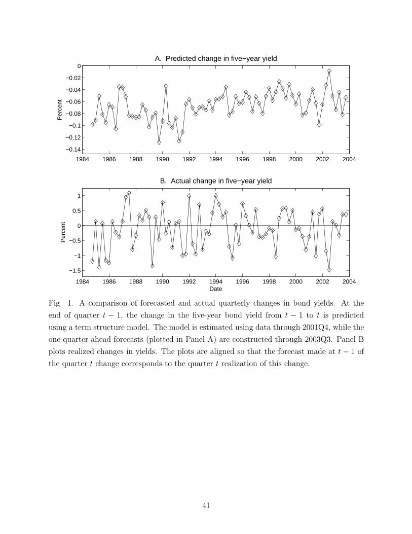
1984 1986 1988 1990 1992 1994 1996 1998 2000 2002 2004

−0.14

−0.12

−0.1

−0.08

−0.06

−0.04

−0.02

0P

erce

ntA. Predicted change in five−year yield

1984 1986 1988 1990 1992 1994 1996 1998 2000 2002 2004

−1.5

−1

−0.5

0

0.5

1

Date

Per

cent

B. Actual change in five−year yield

Fig. 1. A comparison of forecasted and actual quarterly changes in bond yields. At the

end of quarter t − 1, the change in the five-year bond yield from t − 1 to t is predicted

using a term structure model. The model is estimated using data through 2001Q4, while the

one-quarter-ahead forecasts (plotted in Panel A) are constructed through 2003Q3. Panel B

plots realized changes in yields. The plots are aligned so that the forecast made at t− 1 of

the quarter t change corresponds to the quarter t realization of this change.

41