TensorFlow

i

TensorFlow

i

About the Tutorial

TensorFlow is an open source machine learning framework for all developers. It is used

for implementing machine learning and deep learning applications. To develop and

research on fascinating ideas on artificial intelligence, Google team created TensorFlow.

TensorFlow is designed in Python programming language, hence it is considered an easy

to understand framework.

Audience

This tutorial has been prepared for python developers who focus on research and

development with various machine learning and deep learning algorithms. The aim of this

tutorial is to describe all TensorFlow objects and methods.

Prerequisites

Before proceeding with this tutorial, you need to have a basic knowledge of any Python

programming language. Knowledge of artificial intelligence concepts will be a plus point.

Copyright & Disclaimer

Copyright 2018 by Tutorials Point (I) Pvt. Ltd.

All the content and graphics published in this e-book are the property of Tutorials Point (I)

Pvt. Ltd. The user of this e-book is prohibited to reuse, retain, copy, distribute or republish

any contents or a part of contents of this e-book in any manner without written consent

of the publisher.

We strive to update the contents of our website and tutorials as timely and as precisely as

possible, however, the contents may contain inaccuracies or errors. Tutorials Point (I) Pvt.

Ltd. provides no guarantee regarding the accuracy, timeliness or completeness of our

website or its contents including this tutorial. If you discover any errors on our website or

in this tutorial, please notify us at contact@tutorialspoint.com

TensorFlow

ii

Table of Contents

About the Tutorial ............................................................................................................................................ i

Audience ........................................................................................................................................................... i

Prerequisites ..................................................................................................................................................... i

Copyright & Disclaimer ..................................................................................................................................... i

Table of Contents ............................................................................................................................................ ii

1. TensorFlow — Introduction ...................................................................................................................... 1

Why is TensorFlow So Popular? ...................................................................................................................... 1

2. TensorFlow — Installation ........................................................................................................................ 3

3. TensorFlow — Understanding Artificial Intelligence ................................................................................. 8

Supervised Learning ........................................................................................................................................ 9

Unsupervised Learning .................................................................................................................................... 9

4. TensorFlow — Mathematical Foundations .............................................................................................. 11

Vector ............................................................................................................................................................ 11

Mathematical Computations ......................................................................................................................... 12

5. TensorFlow — Machine Learning and Deep Learning .............................................................................. 15

Machine Learning .......................................................................................................................................... 15

Deep Learning ................................................................................................................................................ 15

Difference between Machine Learning and Deep learning ........................................................................... 16

Applications of Machine Learning and Deep Learning .................................................................................. 17

6. TensorFlow — Basics............................................................................................................................... 19

Tensor Data Structure ................................................................................................................................... 19

Various Dimensions of TensorFlow ............................................................................................................... 20

Two dimensional Tensors .............................................................................................................................. 21

Tensor Handling and Manipulations ............................................................................................................. 23

7. TensorFlow — Convolutional Neural Networks....................................................................................... 25

Convolutional Neural Networks .................................................................................................................... 25

TensorFlow

iii

TensorFlow Implementation of CNN ............................................................................................................. 27

8. TensorFlow — Recurrent Neural Networks ............................................................................................. 31

Recurrent Neural Network Implementation with TensorFlow ...................................................................... 32

9. TensorFlow — TensorBoard Visualization ............................................................................................... 36

10. TensorFlow — Word Embedding ............................................................................................................. 38

Word2vec ...................................................................................................................................................... 38

11. TensorFlow — Single Layer Perceptron ................................................................................................... 42

Single Layer Perceptron ................................................................................................................................. 43

12. TensorFlow — Linear Regression ............................................................................................................ 47

Steps to design an algorithm for linear regression ........................................................................................ 48

13. TensorFlow — TFLearn and its installation .............................................................................................. 50

14. TensorFlow — CNN and RNN Difference ................................................................................................. 52

15. TensorFlow — Keras ............................................................................................................................... 53

16. TensorFlow — Distributed Computing .................................................................................................... 56

17. TensorFlow — Exporting with TensorFlow .............................................................................................. 58

18. TensorFlow — Multi-Layer Perceptron Learning ..................................................................................... 59

19. TensorFlow — Hidden Layers of Perceptron ........................................................................................... 63

20. TensorFlow — Optimizers in TensorFlow ................................................................................................ 67

21. TensorFlow — XOR Implementation ....................................................................................................... 68

22. TensorFlow — Gradient Descent Optimization ....................................................................................... 71

23. TensorFlow — Forming Graphs ............................................................................................................... 73

24. TensorFlow — Image Recognition using TensorFlow ............................................................................... 77

25. TensorFlow — Recommendations for Neural Network Training ............................................................. 82

TensorFlow

1

TensorFlow is a software library or framework, designed by the Google team to implement

machine learning and deep learning concepts in the easiest manner. It combines the

computational algebra of optimization techniques for easy calculation of many

mathematical expressions.

The official website of TensorFlow is mentioned below:

https://www.tensorflow.org/

Let us now consider the following important features of TensorFlow:

It includes a feature of that defines, optimizes and calculates mathematical

expressions easily with the help of multi-dimensional arrays called tensors.

It includes a programming support of deep neural networks and machine learning

techniques.

It includes a high scalable feature of computation with various data sets.

TensorFlow uses GPU computing, automating management. It also includes a

unique feature of optimization of same memory and the data used.

Why is TensorFlow So Popular?

TensorFlow is well-documented and includes plenty of machine learning libraries. It offers

a few important functionalities and methods for the same.

TensorFlow is also called a “Google” product. It includes a variety of machine learning and

deep learning algorithms. TensorFlow can train and run deep neural networks for

1. TensorFlow — Introduction

TensorFlow

2

handwritten digit classification, image recognition, word embedding and creation of

various sequence models.

TensorFlow

3

To install TensorFlow, it is important to have “Python” installed in your system. Python

version 3.4+ is considered the best to start with TensorFlow installation.

Consider the following steps to install TensorFlow in Windows operating system.

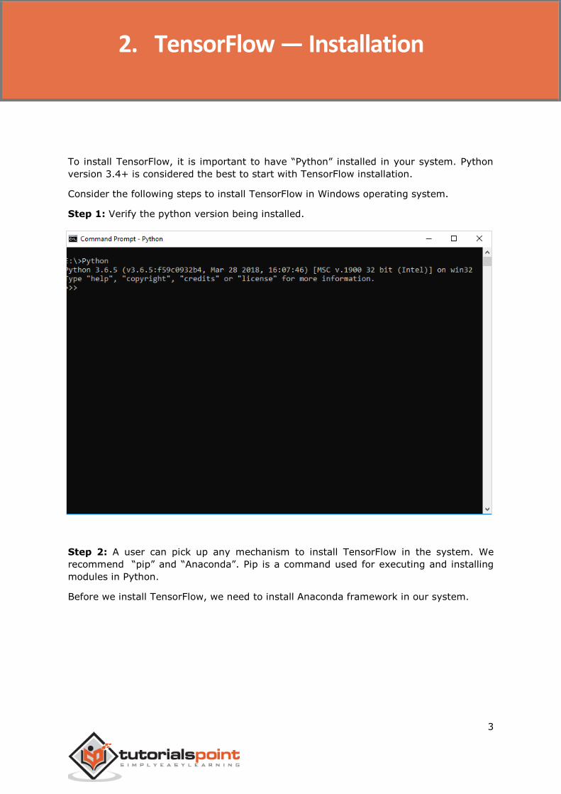
Step 1: Verify the python version being installed.

Step 2: A user can pick up any mechanism to install TensorFlow in the system. We

recommend “pip” and “Anaconda”. Pip is a command used for executing and installing

modules in Python.

Before we install TensorFlow, we need to install Anaconda framework in our system.

2. TensorFlow — Installation

TensorFlow

4

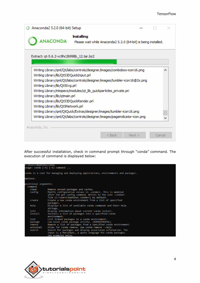
After successful installation, check in command prompt through “conda” command. The

execution of command is displayed below:

TensorFlow

5

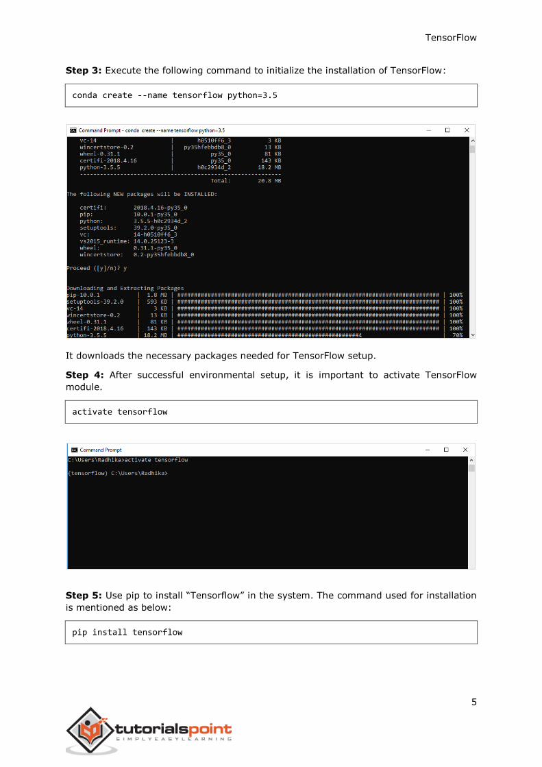
Step 3: Execute the following command to initialize the installation of TensorFlow:

conda create --name tensorflow python=3.5

It downloads the necessary packages needed for TensorFlow setup.

Step 4: After successful environmental setup, it is important to activate TensorFlow

module.

activate tensorflow

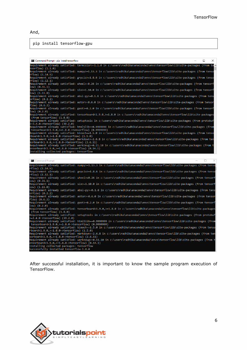
Step 5: Use pip to install “Tensorflow” in the system. The command used for installation

is mentioned as below:

pip install tensorflow

TensorFlow

6

And,

pip install tensorflow-gpu

After successful installation, it is important to know the sample program execution of

TensorFlow.

TensorFlow

7

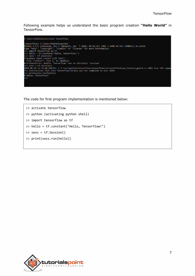
Following example helps us understand the basic program creation “Hello World” in

TensorFlow.

The code for first program implementation is mentioned below:

>> activate tensorflow

>> python (activating python shell)

>> import tensorflow as tf

>> hello = tf.constant(‘Hello, Tensorflow!’)

>> sess = tf.Session()

>> print(sess.run(hello))

TensorFlow

8

Artificial Intelligence includes the simulation process of human intelligence by machines

and special computer systems. The examples of artificial intelligence include learning,

reasoning and self-correction. Applications of AI include speech recognition, expert

systems, and image recognition and machine vision.

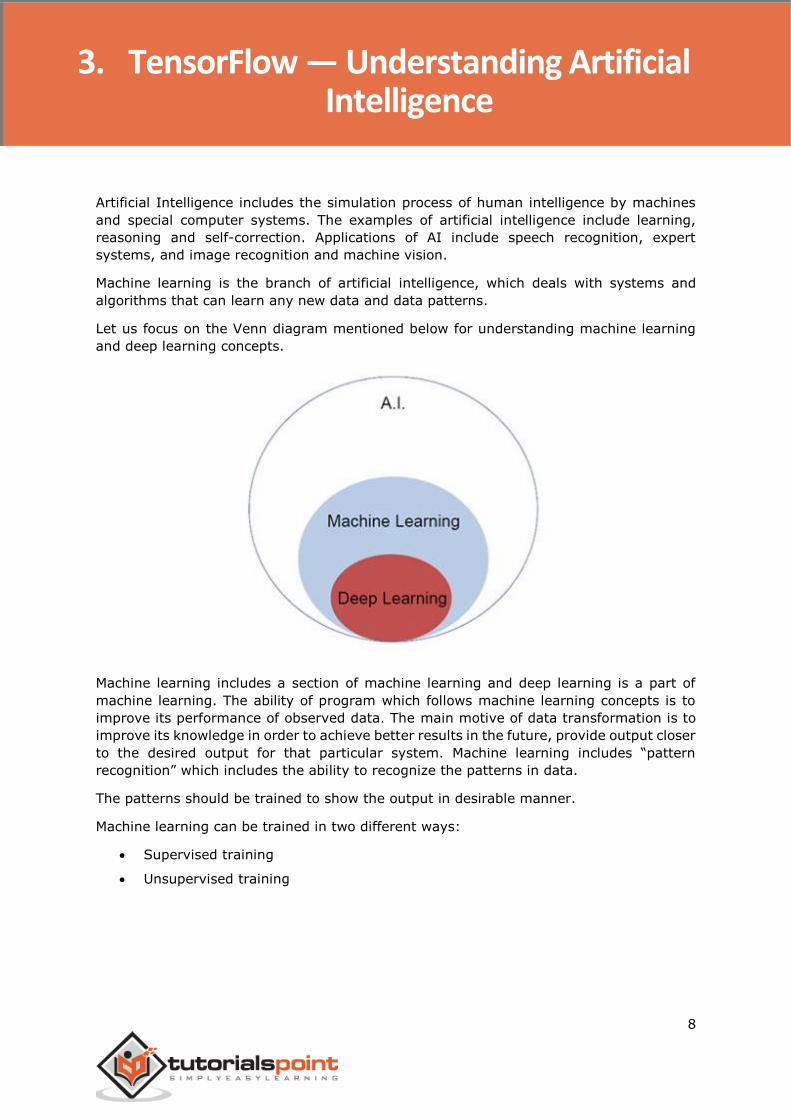
Machine learning is the branch of artificial intelligence, which deals with systems and

algorithms that can learn any new data and data patterns.

Let us focus on the Venn diagram mentioned below for understanding machine learning

and deep learning concepts.

Machine learning includes a section of machine learning and deep learning is a part of

machine learning. The ability of program which follows machine learning concepts is to

improve its performance of observed data. The main motive of data transformation is to

improve its knowledge in order to achieve better results in the future, provide output closer

to the desired output for that particular system. Machine learning includes “pattern

recognition” which includes the ability to recognize the patterns in data.

The patterns should be trained to show the output in desirable manner.

Machine learning can be trained in two different ways:

Supervised training

Unsupervised training

3. TensorFlow — Understanding Artificial Intelligence

TensorFlow

9

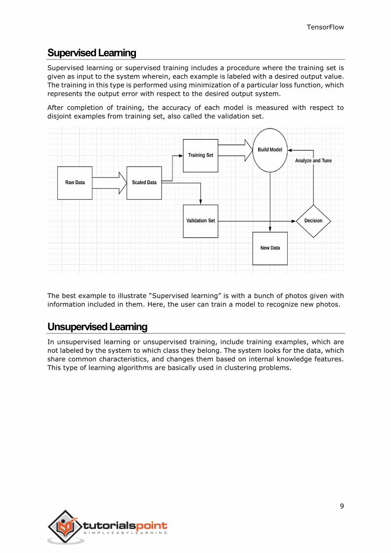
Supervised Learning

Supervised learning or supervised training includes a procedure where the training set is

given as input to the system wherein, each example is labeled with a desired output value.

The training in this type is performed using minimization of a particular loss function, which

represents the output error with respect to the desired output system.

After completion of training, the accuracy of each model is measured with respect to

disjoint examples from training set, also called the validation set.

The best example to illustrate “Supervised learning” is with a bunch of photos given with

information included in them. Here, the user can train a model to recognize new photos.

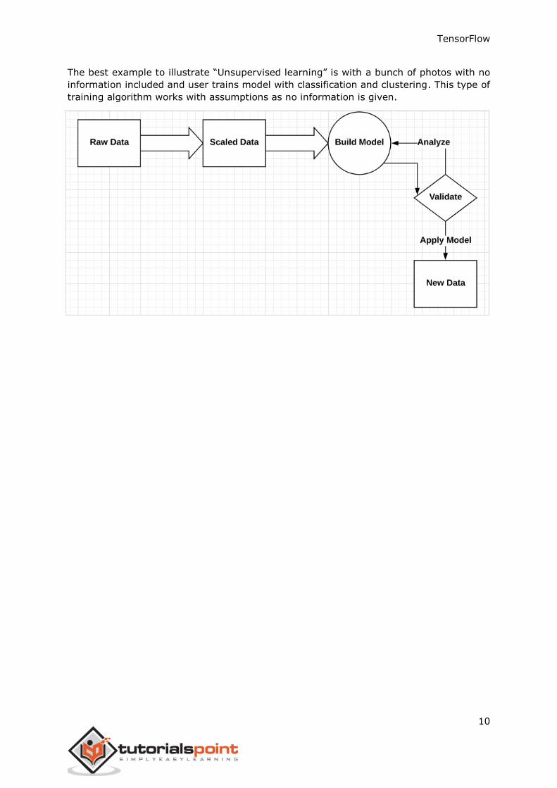
Unsupervised Learning

In unsupervised learning or unsupervised training, include training examples, which are

not labeled by the system to which class they belong. The system looks for the data, which

share common characteristics, and changes them based on internal knowledge features.

This type of learning algorithms are basically used in clustering problems.

TensorFlow

10

The best example to illustrate “Unsupervised learning” is with a bunch of photos with no

information included and user trains model with classification and clustering. This type of

training algorithm works with assumptions as no information is given.

TensorFlow

11

It is important to understand mathematical concepts needed for TensorFlow before

creating the basic application in TensorFlow. Mathematics is considered as the heart of

any machine learning algorithm. It is with the help of core concepts of Mathematics, a

solution for specific machine learning algorithm is defined.

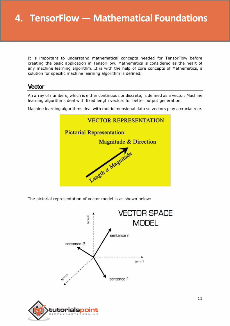
Vector

An array of numbers, which is either continuous or discrete, is defined as a vector. Machine

learning algorithms deal with fixed length vectors for better output generation.

Machine learning algorithms deal with multidimensional data so vectors play a crucial role.

The pictorial representation of vector model is as shown below:

4. TensorFlow — Mathematical Foundations

TensorFlow

12

Scalar

Scalar can be defined as one-dimensional vector. Scalars are those, which include only

magnitude and no direction. With scalars, we are only concerned with the magnitude.

Examples of scalar include weight and height parameters of children.

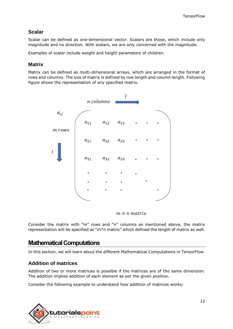
Matrix

Matrix can be defined as multi-dimensional arrays, which are arranged in the format of

rows and columns. The size of matrix is defined by row length and column length. Following

figure shows the representation of any specified matrix.

Consider the matrix with “m” rows and “n” columns as mentioned above, the matrix

representation will be specified as “m*n matrix” which defined the length of matrix as well.

Mathematical Computations

In this section, we will learn about the different Mathematical Computations in TensorFlow.

Addition of matrices

Addition of two or more matrices is possible if the matrices are of the same dimension.

The addition implies addition of each element as per the given position.

Consider the following example to understand how addition of matrices works:

TensorFlow

13

Subtraction of matrices

The subtraction of matrices operates in similar fashion like the addition of two matrices.

The user can subtract two matrices provided the dimensions are equal.

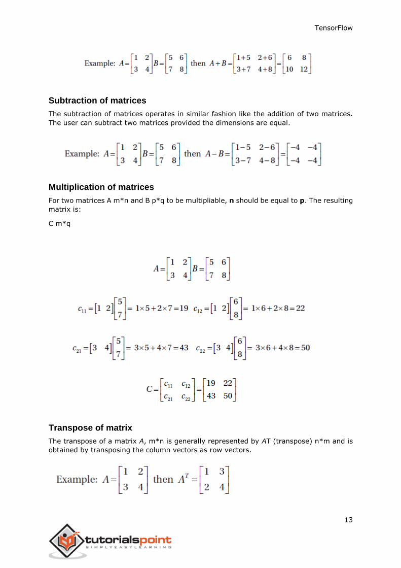
Multiplication of matrices

For two matrices A m*n and B p*q to be multipliable, n should be equal to p. The resulting

matrix is:

C m*q

Transpose of matrix

The transpose of a matrix A, m*n is generally represented by AT (transpose) n*m and is

obtained by transposing the column vectors as row vectors.

TensorFlow

14

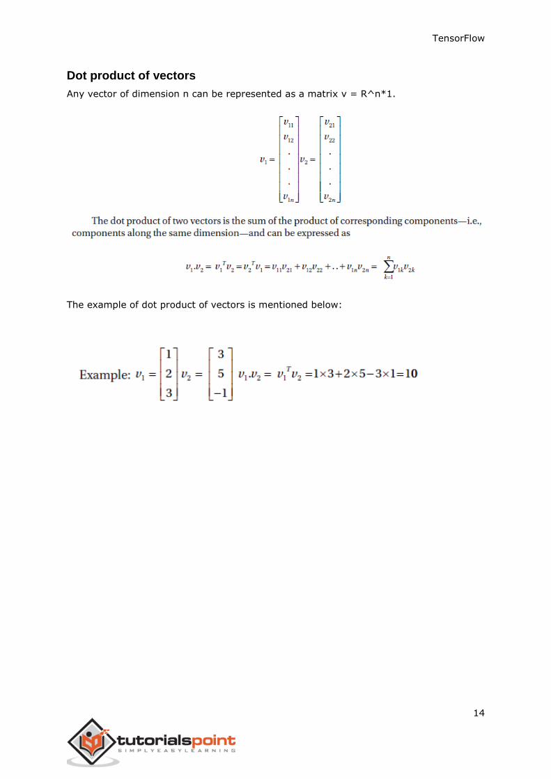
Dot product of vectors

Any vector of dimension n can be represented as a matrix v = R^n*1.

The example of dot product of vectors is mentioned below:

TensorFlow

15

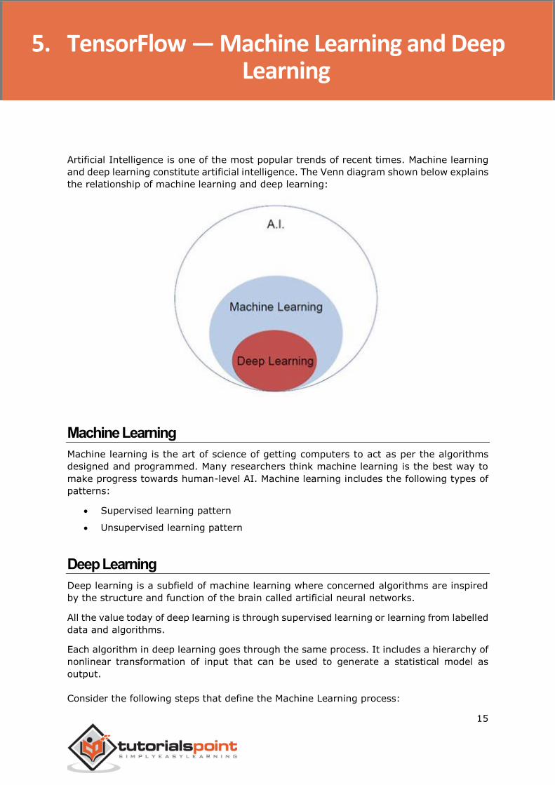
Artificial Intelligence is one of the most popular trends of recent times. Machine learning

and deep learning constitute artificial intelligence. The Venn diagram shown below explains

the relationship of machine learning and deep learning:

Machine Learning

Machine learning is the art of science of getting computers to act as per the algorithms

designed and programmed. Many researchers think machine learning is the best way to

make progress towards human-level AI. Machine learning includes the following types of

patterns:

Supervised learning pattern

Unsupervised learning pattern

Deep Learning

Deep learning is a subfield of machine learning where concerned algorithms are inspired

by the structure and function of the brain called artificial neural networks.

All the value today of deep learning is through supervised learning or learning from labelled

data and algorithms.

Each algorithm in deep learning goes through the same process. It includes a hierarchy of

nonlinear transformation of input that can be used to generate a statistical model as

output.

Consider the following steps that define the Machine Learning process:

5. TensorFlow — Machine Learning and Deep Learning

TensorFlow

16

Identifies relevant data sets and prepares them for analysis.

Chooses the type of algorithm to use.

Builds an analytical model based on the algorithm used.

Trains the model on test data sets, revising it as needed.

Runs the model to generate test scores.

Difference between Machine Learning and Deep learning

In this section, we will learn about the difference between Machine Learning and Deep

Learning.

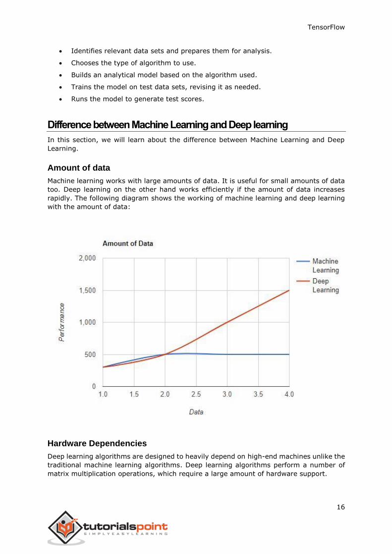
Amount of data

Machine learning works with large amounts of data. It is useful for small amounts of data

too. Deep learning on the other hand works efficiently if the amount of data increases

rapidly. The following diagram shows the working of machine learning and deep learning

with the amount of data:

Hardware Dependencies

Deep learning algorithms are designed to heavily depend on high-end machines unlike the

traditional machine learning algorithms. Deep learning algorithms perform a number of

matrix multiplication operations, which require a large amount of hardware support.

TensorFlow

17

Feature Engineering

Feature engineering is the process of putting domain knowledge into specified features to

reduce the complexity of data and make patterns that are visible to learning algorithms it

works.

Example: Traditional machine learning patterns focus on pixels and other attributes

needed for feature engineering process. Deep learning algorithms focus on high-level

features from data. It reduces the task of developing new feature extractor of every new

problem.

Problem Solving Approach

The traditional machine learning algorithms follow a standard procedure to solve the

problem. It breaks the problem into parts, solve each one of them and combine them to

get the required result. Deep learning focusses in solving the problem from end to end

instead of breaking them into divisions.

Execution Time

Execution time is the amount of time required to train an algorithm. Deep learning requires

a lot of time to train as it includes a lot of parameters which takes a longer time than

usual. Machine learning algorithm comparatively requires less execution time.

Interpretability

Interpretability is the major factor for comparison of machine learning and deep learning

algorithms. The main reason is that deep learning is still given a second thought before its

usage in industry.

Applications of Machine Learning and Deep Learning

In this section, we will learn about the different applications of Machine Learning and Deep

Learning.

Computer vision which is used for facial recognition and attendance mark through

fingerprints or vehicle identification through number plate.

Information Retrieval from search engines like text search for image search.

Automated email marketing with specified target identification.

Medical diagnosis of cancer tumors or anomaly identification of any chronic disease.

Natural language processing for applications like photo tagging. The best example

to explain this scenario is used in Facebook.

Online Advertising.

TensorFlow

18

Future Trends

With the increasing trend of using data science and machine learning in the

industry, it will become important for each organization to inculcate machine

learning in their businesses.

Deep learning is gaining more importance than machine learning. Deep learning is

proving to be one of the best techniques in state-of-art performance.

Machine learning and deep learning will prove beneficial in research and academics

field.

Conclusion

In this article, we had an overview of machine learning and deep learning with illustrations

and differences also focusing on future trends. Many of AI applications utilize machine

learning algorithms primarily to drive self-service, increase agent productivity and

workflows more reliable. Machine learning and deep learning algorithms include an exciting

prospect for many businesses and industry leaders.

TensorFlow

19

In this chapter, we will learn about the basics of TensorFlow. We will begin by

understanding the data structure of tensor.

Tensor Data Structure

Tensors are used as the basic data structures in TensorFlow language. Tensors represent

the connecting edges in any flow diagram called the Data Flow Graph. Tensors are defined

as multidimensional array or list.

Tensors are identified by the following three parameters:

Rank

Unit of dimensionality described within tensor is called rank. It identifies the number of

dimensions of the tensor. A rank of a tensor can be described as the order or n-dimensions

of a tensor defined.

Shape

The number of rows and columns together define the shape of Tensor.

Type

Type describes the data type assigned to Tensor’s elements.

A user needs to consider the following activities for building a Tensor:

Build an n-dimensional array

Convert the n-dimensional array.

6. TensorFlow — Basics

TensorFlow

20

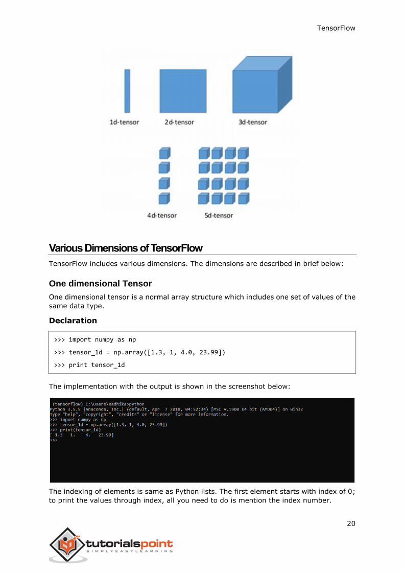
Various Dimensions of TensorFlow

TensorFlow includes various dimensions. The dimensions are described in brief below:

One dimensional Tensor

One dimensional tensor is a normal array structure which includes one set of values of the

same data type.

Declaration

>>> import numpy as np

>>> tensor_1d = np.array([1.3, 1, 4.0, 23.99])

>>> print tensor_1d

The implementation with the output is shown in the screenshot below:

The indexing of elements is same as Python lists. The first element starts with index of 0;

to print the values through index, all you need to do is mention the index number.

TensorFlow

21

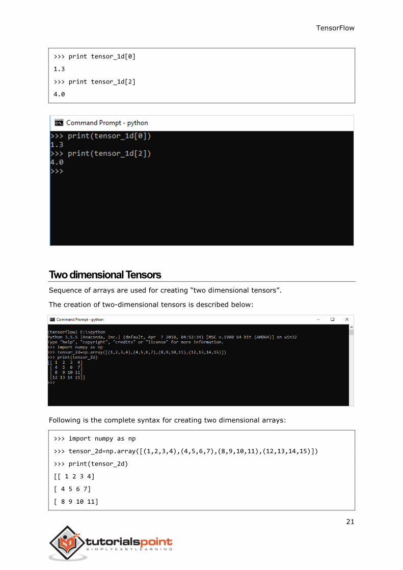
>>> print tensor_1d[0]

1.3

>>> print tensor_1d[2]

4.0

Two dimensional Tensors

Sequence of arrays are used for creating “two dimensional tensors”.

The creation of two-dimensional tensors is described below:

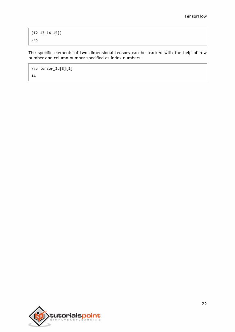
Following is the complete syntax for creating two dimensional arrays:

>>> import numpy as np

>>> tensor_2d=np.array([(1,2,3,4),(4,5,6,7),(8,9,10,11),(12,13,14,15)])

>>> print(tensor_2d)

[[ 1 2 3 4]

[ 4 5 6 7]

[ 8 9 10 11]

TensorFlow

22

[12 13 14 15]]

>>>

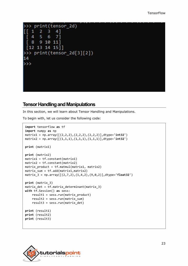
The specific elements of two dimensional tensors can be tracked with the help of row

number and column number specified as index numbers.

>>> tensor_2d[3][2]

14

TensorFlow

23

Tensor Handling and Manipulations

In this section, we will learn about Tensor Handling and Manipulations.

To begin with, let us consider the following code:

import tensorflow as tf

import numpy as np

matrix1 = np.array([(2,2,2),(2,2,2),(2,2,2)],dtype='int32')

matrix2 = np.array([(1,1,1),(1,1,1),(1,1,1)],dtype='int32')

print (matrix1)

print (matrix2)

matrix1 = tf.constant(matrix1)

matrix2 = tf.constant(matrix2)

matrix_product = tf.matmul(matrix1, matrix2)

matrix_sum = tf.add(matrix1,matrix2)

matrix_3 = np.array([(2,7,2),(1,4,2),(9,0,2)],dtype='float32')

print (matrix_3)

matrix_det = tf.matrix_determinant(matrix_3)

with tf.Session() as sess:

result1 = sess.run(matrix_product)

result2 = sess.run(matrix_sum)

result3 = sess.run(matrix_det)

print (result1)

print (result2)

print (result3)

TensorFlow

24

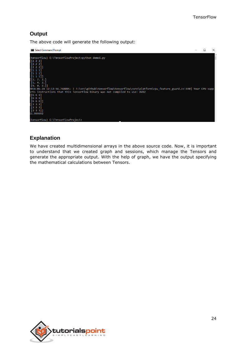
Output

The above code will generate the following output:

Explanation

We have created multidimensional arrays in the above source code. Now, it is important

to understand that we created graph and sessions, which manage the Tensors and

generate the appropriate output. With the help of graph, we have the output specifying

the mathematical calculations between Tensors.

TensorFlow

25

After understanding machine-learning concepts, we can now shift our focus to deep

learning concepts. Deep learning is a division of machine learning and is considered as a

crucial step taken by researchers in recent decades. The examples of deep learning

implementation include applications like image recognition and speech recognition.

Following are the two important types of deep neural networks:

Convolutional Neural Networks

Recurrent Neural Networks

In this chapter, we will focus on the CNN, Convolutional Neural Networks.

Convolutional Neural Networks

Convolutional Neural networks are designed to process data through multiple layers of

arrays. This type of neural networks is used in applications like image recognition or face

recognition. The primary difference between CNN and any other ordinary neural network

is that CNN takes input as a two-dimensional array and operates directly on the images

rather than focusing on feature extraction which other neural networks focus on.

The dominant approach of CNN includes solutions for problems of recognition. Top

companies like Google and Facebook have invested in research and development towards

recognition projects to get activities done with greater speed.

A convolutional neural network uses three basic ideas:

Local respective fields

Convolution

Pooling

Let us understand these ideas in detail.

CNN utilizes spatial correlations that exist within the input data. Each concurrent layer of

a neural network connects some input neurons. This specific region is called local receptive

field. Local receptive field focusses on the hidden neurons. The hidden neurons process

the input data inside the mentioned field not realizing the changes outside the specific

boundary.

7. TensorFlow — Convolutional Neural Networks

TensorFlow

26

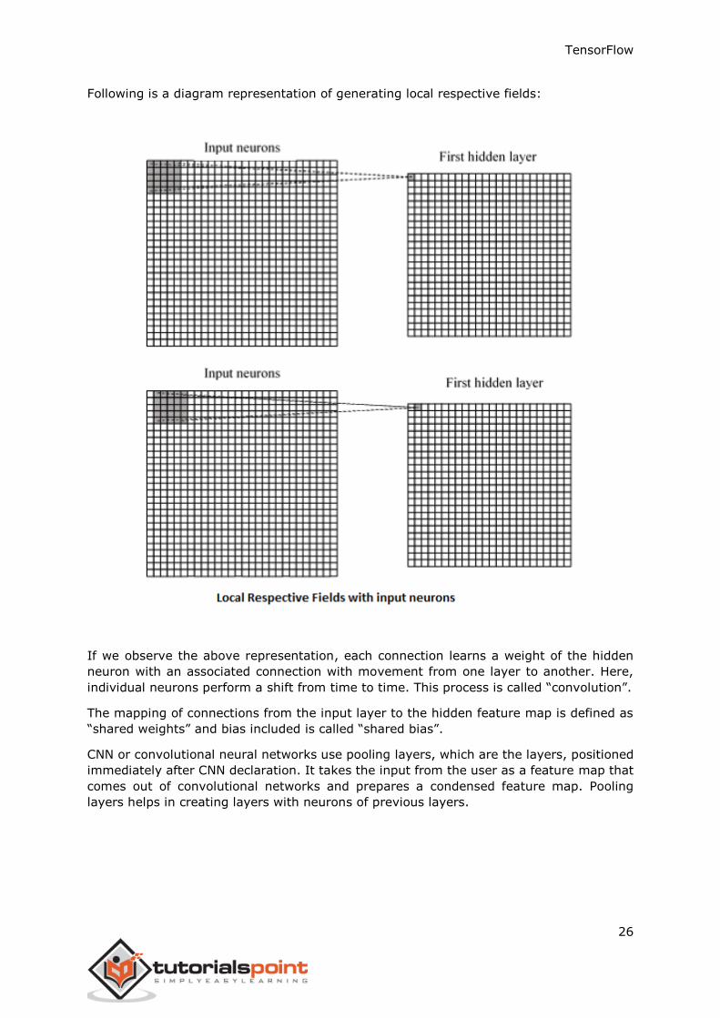
Following is a diagram representation of generating local respective fields:

If we observe the above representation, each connection learns a weight of the hidden

neuron with an associated connection with movement from one layer to another. Here,

individual neurons perform a shift from time to time. This process is called “convolution”.

The mapping of connections from the input layer to the hidden feature map is defined as

“shared weights” and bias included is called “shared bias”.

CNN or convolutional neural networks use pooling layers, which are the layers, positioned

immediately after CNN declaration. It takes the input from the user as a feature map that

comes out of convolutional networks and prepares a condensed feature map. Pooling

layers helps in creating layers with neurons of previous layers.

TensorFlow

27

TensorFlow Implementation of CNN

In this section, we will learn about the TensorFlow implementation of CNN. The steps,

which require the execution and proper dimension of the entire network, are as shown

below:

Step 1: Include the necessary modules for TensorFlow and the data set modules, which

are needed to compute the CNN model.

import tensorflow as tf

import numpy as np

from tensorflow.examples.tutorials.mnist import input_data

Step 2: Declare a function called run_cnn(), which includes various parameters and

optimization variables with declaration of data placeholders. These optimization variables

will declare the training pattern.

def run_cnn():

mnist = input_data.read_data_sets("MNIST_data/", one_hot=True)

learning_rate = 0.0001

epochs = 10

batch_size = 50

Step 3: In this step, we will declare the training data placeholders with input parameters

- for 28 x 28 pixels = 784. This is the flattened image data that is drawn from

mnist.train.nextbatch().

We can reshape the tensor according to our requirements. The first value (-1) tells

function to dynamically shape that dimension based on the amount of data passed to it.

The two middle dimensions are set to the image size (i.e. 28 x 28).

x = tf.placeholder(tf.float32, [None, 784])

x_shaped = tf.reshape(x, [-1, 28, 28, 1])

y = tf.placeholder(tf.float32, [None, 10])

Step 4: Now it is important to create some convolutional layers:

layer1 = create_new_conv_layer(x_shaped, 1, 32, [5, 5], [2, 2], name='layer1')

layer2 = create_new_conv_layer(layer1, 32, 64, [5, 5], [2, 2],

name='layer2')

TensorFlow

28

Step 5: Let us flatten the output ready for the fully connected output stage - after two

layers of stride 2 pooling with the dimensions of 28 x 28, to dimension of 14 x 14 or

minimum 7 x 7 x,y co-ordinates, but with 64 output channels. To create the fully connected

with "dense" layer, the new shape needs to be [-1, 7 x 7 x 64]. We can set up some

weights and bias values for this layer, then activate with ReLU.

flattened = tf.reshape(layer2, [-1, 7 * 7 * 64])

wd1 = tf.Variable(tf.truncated_normal([7 * 7 * 64, 1000], stddev=0.03),

name='wd1')

bd1 = tf.Variable(tf.truncated_normal([1000], stddev=0.01), name='bd1')

dense_layer1 = tf.matmul(flattened, wd1) + bd1

dense_layer1 = tf.nn.relu(dense_layer1)

Step 6: Another layer with specific softmax activations with the required optimizer defines

the accuracy assessment, which makes the setup of initialization operator.

wd2 = tf.Variable(tf.truncated_normal([1000, 10], stddev=0.03), name='wd2')

bd2 = tf.Variable(tf.truncated_normal([10], stddev=0.01), name='bd2')

dense_layer2 = tf.matmul(dense_layer1, wd2) + bd2

y_ = tf.nn.softmax(dense_layer2)

cross_entropy =

tf.reduce_mean(tf.nn.softmax_cross_entropy_with_logits(logits=dense_layer2,

labels=y))

optimiser =

tf.train.AdamOptimizer(learning_rate=learning_rate).minimize(cross_entropy)

correct_prediction = tf.equal(tf.argmax(y, 1), tf.argmax(y_, 1))

accuracy = tf.reduce_mean(tf.cast(correct_prediction, tf.float32))

init_op = tf.global_variables_initializer()

Step 7: We should set up recording variables. This adds up a summary to store the

accuracy of data.

tf.summary.scalar('accuracy', accuracy)

merged = tf.summary.merge_all()

TensorFlow

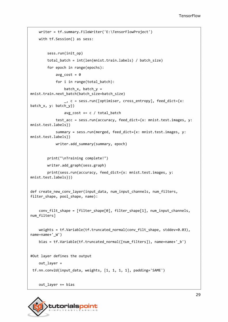
29

writer = tf.summary.FileWriter('E:\TensorFlowProject')

with tf.Session() as sess:

sess.run(init_op)

total_batch = int(len(mnist.train.labels) / batch_size)

for epoch in range(epochs):

avg_cost = 0

for i in range(total_batch):

batch_x, batch_y =

mnist.train.next_batch(batch_size=batch_size)

_, c = sess.run([optimiser, cross_entropy], feed_dict={x:

batch_x, y: batch_y})

avg_cost += c / total_batch

test_acc = sess.run(accuracy, feed_dict={x: mnist.test.images, y:

mnist.test.labels})

summary = sess.run(merged, feed_dict={x: mnist.test.images, y:

mnist.test.labels})

writer.add_summary(summary, epoch)

print("\nTraining complete!")

writer.add_graph(sess.graph)

print(sess.run(accuracy, feed_dict={x: mnist.test.images, y:

mnist.test.labels}))

def create_new_conv_layer(input_data, num_input_channels, num_filters,

filter_shape, pool_shape, name):

conv_filt_shape = [filter_shape[0], filter_shape[1], num_input_channels,

num_filters]

weights = tf.Variable(tf.truncated_normal(conv_filt_shape, stddev=0.03),

name=name+'_W')

bias = tf.Variable(tf.truncated_normal([num_filters]), name=name+'_b')

#Out layer defines the output

out_layer =

tf.nn.conv2d(input_data, weights, [1, 1, 1, 1], padding='SAME')

out_layer += bias

TensorFlow

30

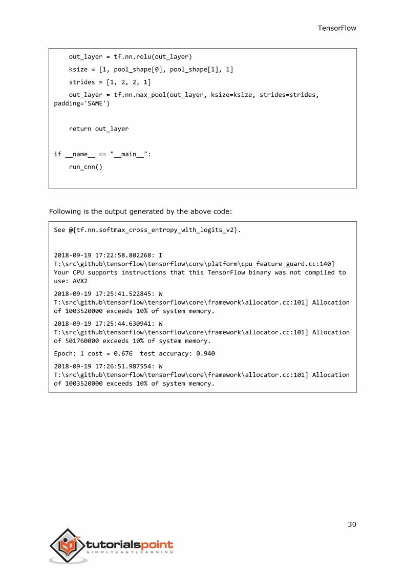
out_layer = tf.nn.relu(out_layer)

ksize = [1, pool_shape[0], pool_shape[1], 1]

strides = [1, 2, 2, 1]

out_layer = tf.nn.max_pool(out_layer, ksize=ksize, strides=strides,

padding='SAME')

return out_layer

if __name__ == "__main__":

run_cnn()

Following is the output generated by the above code:

See @{tf.nn.softmax_cross_entropy_with_logits_v2}.

2018-09-19 17:22:58.802268: I

T:\src\github\tensorflow\tensorflow\core\platform\cpu_feature_guard.cc:140]

Your CPU supports instructions that this TensorFlow binary was not compiled to

use: AVX2

2018-09-19 17:25:41.522845: W

T:\src\github\tensorflow\tensorflow\core\framework\allocator.cc:101] Allocation

of 1003520000 exceeds 10% of system memory.

2018-09-19 17:25:44.630941: W

T:\src\github\tensorflow\tensorflow\core\framework\allocator.cc:101] Allocation

of 501760000 exceeds 10% of system memory.

Epoch: 1 cost = 0.676 test accuracy: 0.940

2018-09-19 17:26:51.987554: W

T:\src\github\tensorflow\tensorflow\core\framework\allocator.cc:101] Allocation

of 1003520000 exceeds 10% of system memory.

TensorFlow

31

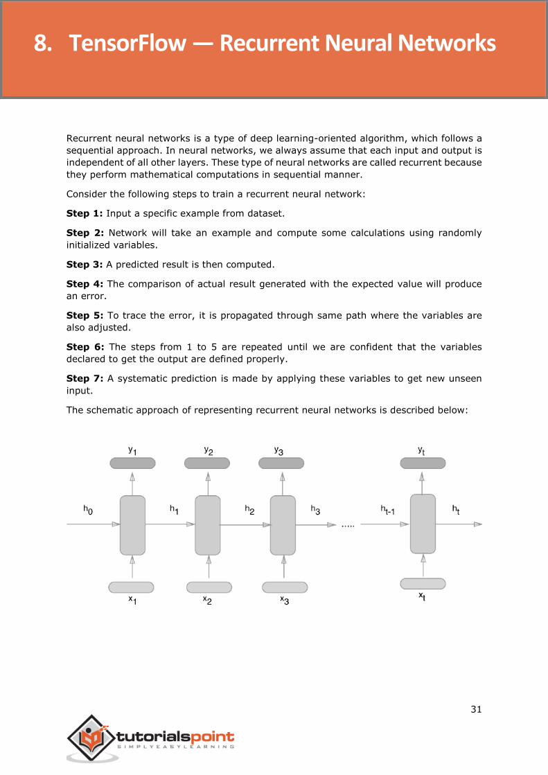
Recurrent neural networks is a type of deep learning-oriented algorithm, which follows a

sequential approach. In neural networks, we always assume that each input and output is

independent of all other layers. These type of neural networks are called recurrent because

they perform mathematical computations in sequential manner.

Consider the following steps to train a recurrent neural network:

Step 1: Input a specific example from dataset.

Step 2: Network will take an example and compute some calculations using randomly

initialized variables.

Step 3: A predicted result is then computed.

Step 4: The comparison of actual result generated with the expected value will produce

an error.

Step 5: To trace the error, it is propagated through same path where the variables are

also adjusted.

Step 6: The steps from 1 to 5 are repeated until we are confident that the variables

declared to get the output are defined properly.

Step 7: A systematic prediction is made by applying these variables to get new unseen

input.

The schematic approach of representing recurrent neural networks is described below:

8. TensorFlow — Recurrent Neural Networks

TensorFlow

32

Recurrent Neural Network Implementation with TensorFlow

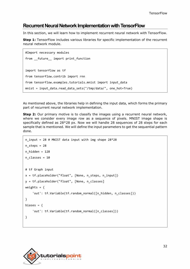
In this section, we will learn how to implement recurrent neural network with TensorFlow.

Step 1: TensorFlow includes various libraries for specific implementation of the recurrent

neural network module.

#Import necessary modules

from __future__ import print_function

import tensorflow as tf

from tensorflow.contrib import rnn

from tensorflow.examples.tutorials.mnist import input_data

mnist = input_data.read_data_sets("/tmp/data/", one_hot=True)

As mentioned above, the libraries help in defining the input data, which forms the primary

part of recurrent neural network implementation.

Step 2: Our primary motive is to classify the images using a recurrent neural network,

where we consider every image row as a sequence of pixels. MNIST image shape is

specifically defined as 28*28 px. Now we will handle 28 sequences of 28 steps for each

sample that is mentioned. We will define the input parameters to get the sequential pattern

done.

n_input = 28 # MNIST data input with img shape 28*28

n_steps = 28

n_hidden = 128

n_classes = 10

# tf Graph input

x = tf.placeholder("float", [None, n_steps, n_input])

y = tf.placeholder("float", [None, n_classes]

weights = {

'out': tf.Variable(tf.random_normal([n_hidden, n_classes]))

}

biases = {

'out': tf.Variable(tf.random_normal([n_classes]))

}

TensorFlow

33

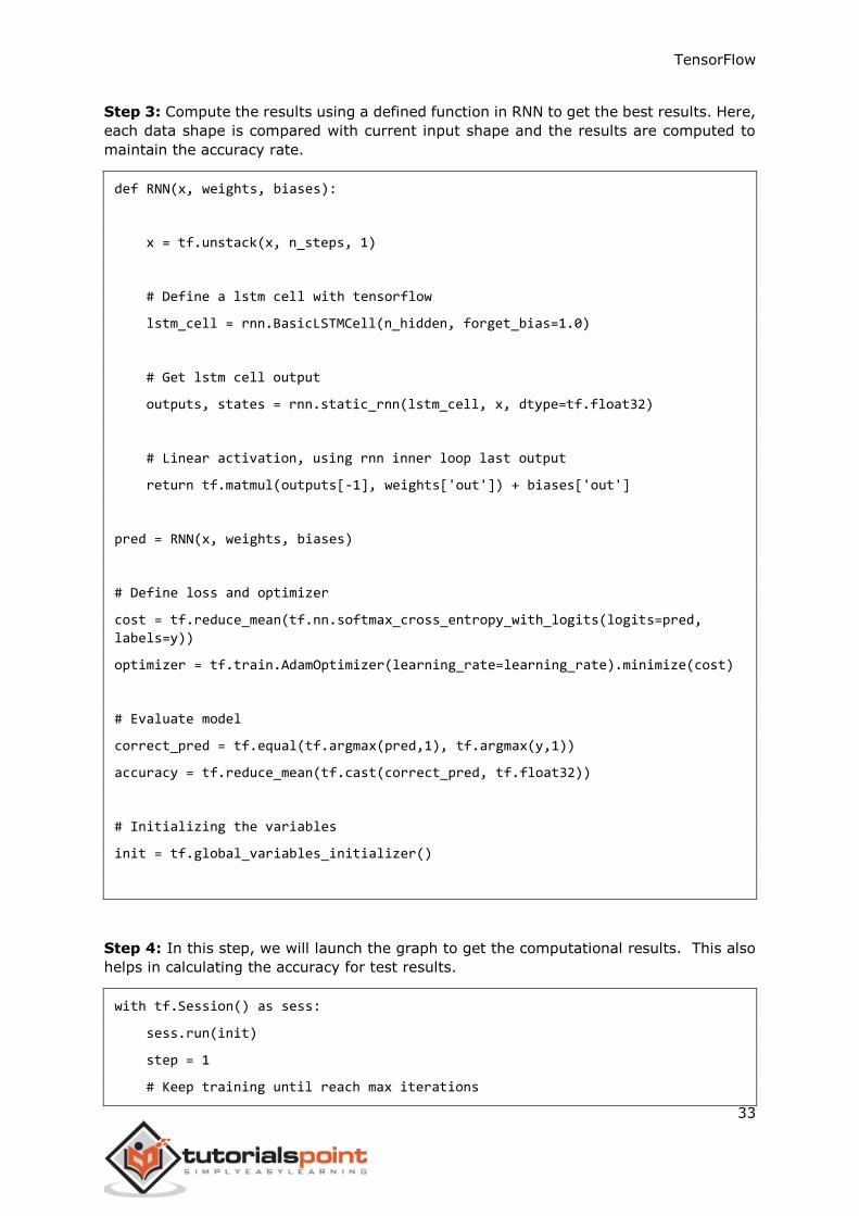
Step 3: Compute the results using a defined function in RNN to get the best results. Here,

each data shape is compared with current input shape and the results are computed to

maintain the accuracy rate.

def RNN(x, weights, biases):

x = tf.unstack(x, n_steps, 1)

# Define a lstm cell with tensorflow

lstm_cell = rnn.BasicLSTMCell(n_hidden, forget_bias=1.0)

# Get lstm cell output

outputs, states = rnn.static_rnn(lstm_cell, x, dtype=tf.float32)

# Linear activation, using rnn inner loop last output

return tf.matmul(outputs[-1], weights['out']) + biases['out']

pred = RNN(x, weights, biases)

# Define loss and optimizer

cost = tf.reduce_mean(tf.nn.softmax_cross_entropy_with_logits(logits=pred,

labels=y))

optimizer = tf.train.AdamOptimizer(learning_rate=learning_rate).minimize(cost)

# Evaluate model

correct_pred = tf.equal(tf.argmax(pred,1), tf.argmax(y,1))

accuracy = tf.reduce_mean(tf.cast(correct_pred, tf.float32))

# Initializing the variables

init = tf.global_variables_initializer()

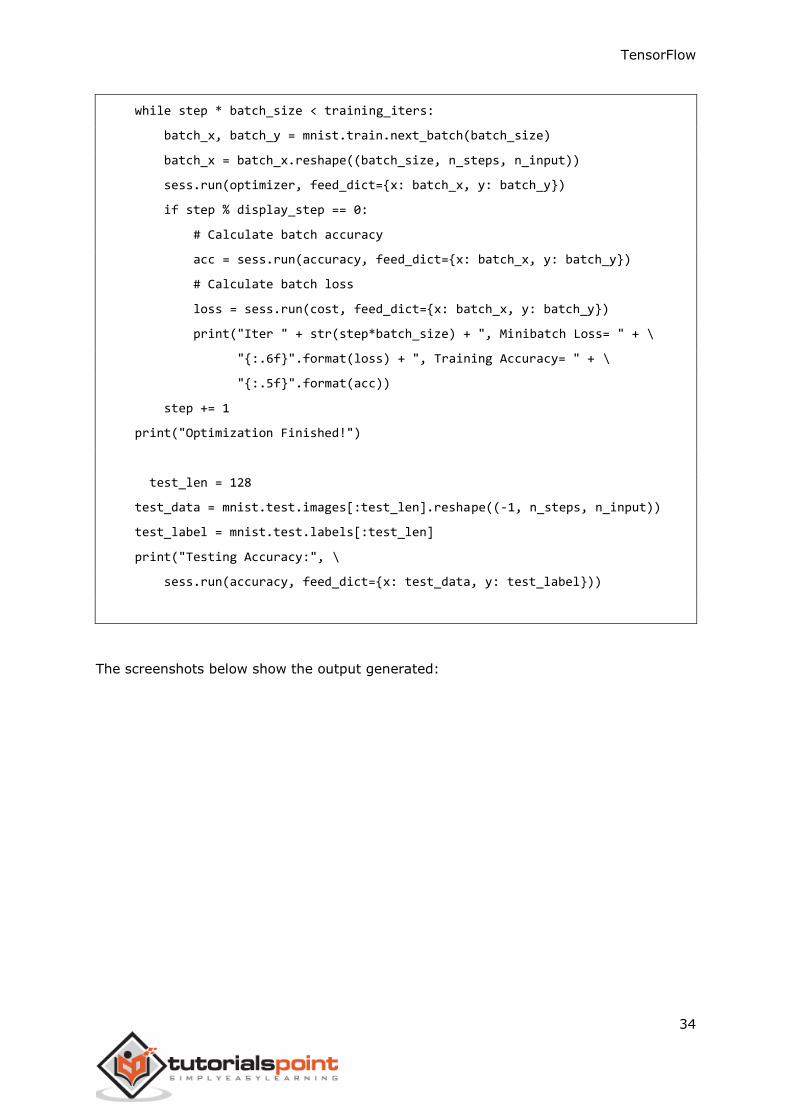
Step 4: In this step, we will launch the graph to get the computational results. This also

helps in calculating the accuracy for test results.

with tf.Session() as sess:

sess.run(init)

step = 1

# Keep training until reach max iterations

TensorFlow

34

while step * batch_size < training_iters:

batch_x, batch_y = mnist.train.next_batch(batch_size)

batch_x = batch_x.reshape((batch_size, n_steps, n_input))

sess.run(optimizer, feed_dict={x: batch_x, y: batch_y})

if step % display_step == 0:

# Calculate batch accuracy

acc = sess.run(accuracy, feed_dict={x: batch_x, y: batch_y})

# Calculate batch loss

loss = sess.run(cost, feed_dict={x: batch_x, y: batch_y})

print("Iter " + str(step*batch_size) + ", Minibatch Loss= " + \

"{:.6f}".format(loss) + ", Training Accuracy= " + \

"{:.5f}".format(acc))

step += 1

print("Optimization Finished!")

test_len = 128

test_data = mnist.test.images[:test_len].reshape((-1, n_steps, n_input))

test_label = mnist.test.labels[:test_len]

print("Testing Accuracy:", \

sess.run(accuracy, feed_dict={x: test_data, y: test_label}))

The screenshots below show the output generated:

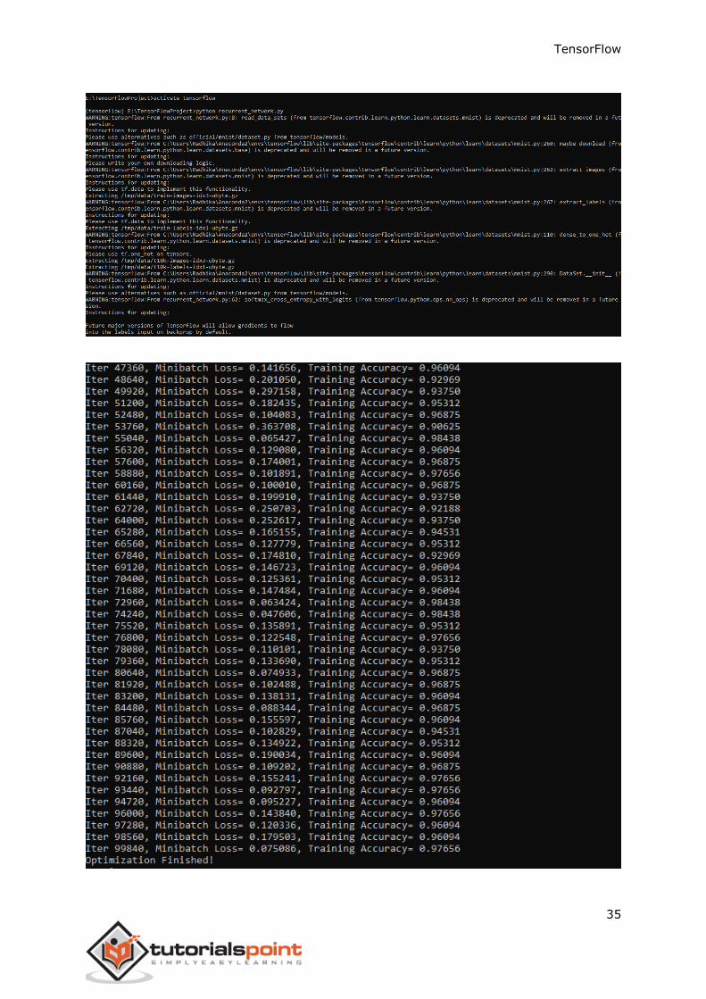
TensorFlow

35

TensorFlow

36

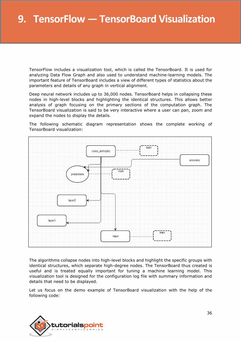
TensorFlow includes a visualization tool, which is called the TensorBoard. It is used for

analyzing Data Flow Graph and also used to understand machine-learning models. The

important feature of TensorBoard includes a view of different types of statistics about the

parameters and details of any graph in vertical alignment.

Deep neural network includes up to 36,000 nodes. TensorBoard helps in collapsing these

nodes in high-level blocks and highlighting the identical structures. This allows better

analysis of graph focusing on the primary sections of the computation graph. The

TensorBoard visualization is said to be very interactive where a user can pan, zoom and

expand the nodes to display the details.

The following schematic diagram representation shows the complete working of

TensorBoard visualization:

The algorithms collapse nodes into high-level blocks and highlight the specific groups with

identical structures, which separate high-degree nodes. The TensorBoard thus created is

useful and is treated equally important for tuning a machine learning model. This

visualization tool is designed for the configuration log file with summary information and

details that need to be displayed.

Let us focus on the demo example of TensorBoard visualization with the help of the

following code:

9. TensorFlow — TensorBoard Visualization

TensorFlow

37

import tensorflow as tf

# Constants creation for TensorBoard visualization

a = tf.constant(10,name="a")

b = tf.constant(90,name="b")

y = tf.Variable(a+b*2,name='y')

model = tf.initialize_all_variables() #Creation of model

with tf.Session() as session:

merged = tf.merge_all_summaries()

writer = tf.train.SummaryWriter("/tmp/tensorflowlogs",session.graph)

session.run(model)

print(session.run(y))

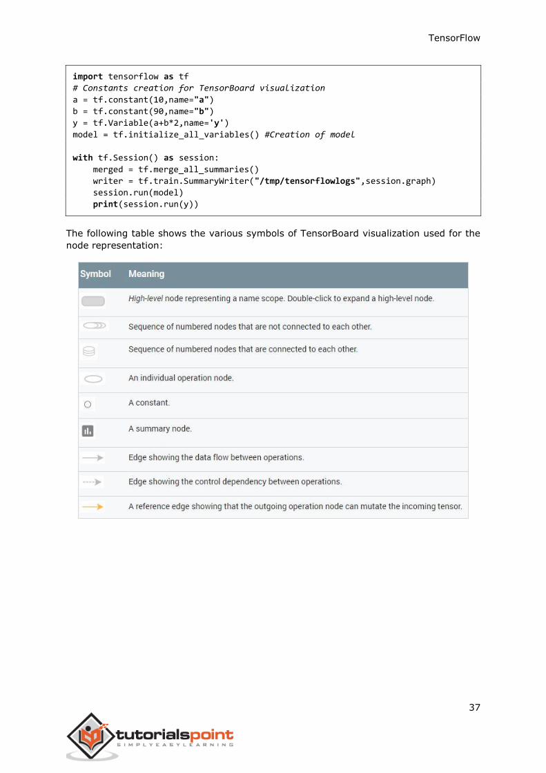
The following table shows the various symbols of TensorBoard visualization used for the

node representation:

TensorFlow

38

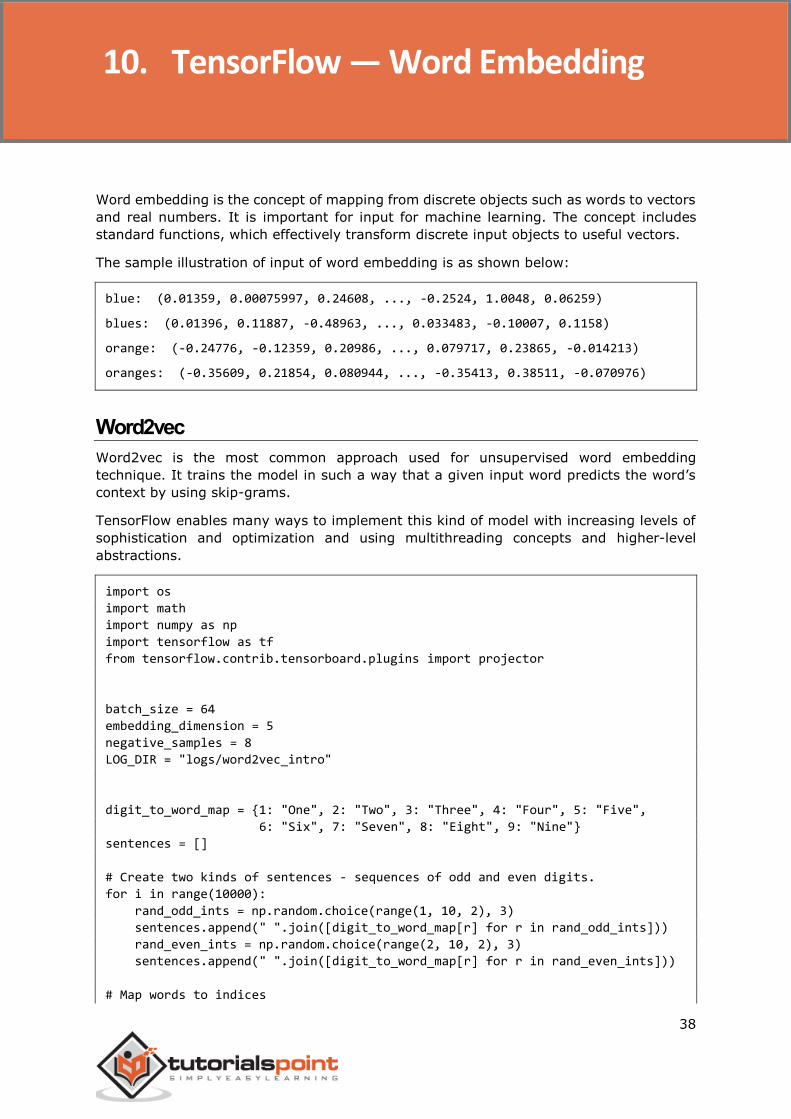
Word embedding is the concept of mapping from discrete objects such as words to vectors

and real numbers. It is important for input for machine learning. The concept includes

standard functions, which effectively transform discrete input objects to useful vectors.

The sample illustration of input of word embedding is as shown below:

blue: (0.01359, 0.00075997, 0.24608, ..., -0.2524, 1.0048, 0.06259)

blues: (0.01396, 0.11887, -0.48963, ..., 0.033483, -0.10007, 0.1158)

orange: (-0.24776, -0.12359, 0.20986, ..., 0.079717, 0.23865, -0.014213)

oranges: (-0.35609, 0.21854, 0.080944, ..., -0.35413, 0.38511, -0.070976)

Word2vec

Word2vec is the most common approach used for unsupervised word embedding

technique. It trains the model in such a way that a given input word predicts the word’s

context by using skip-grams.

TensorFlow enables many ways to implement this kind of model with increasing levels of

sophistication and optimization and using multithreading concepts and higher-level

abstractions.

import os

import math

import numpy as np

import tensorflow as tf

from tensorflow.contrib.tensorboard.plugins import projector

batch_size = 64

embedding_dimension = 5

negative_samples = 8

LOG_DIR = "logs/word2vec_intro"

digit_to_word_map = {1: "One", 2: "Two", 3: "Three", 4: "Four", 5: "Five",

6: "Six", 7: "Seven", 8: "Eight", 9: "Nine"}

sentences = []

# Create two kinds of sentences - sequences of odd and even digits.

for i in range(10000):

rand_odd_ints = np.random.choice(range(1, 10, 2), 3)

sentences.append(" ".join([digit_to_word_map[r] for r in rand_odd_ints]))

rand_even_ints = np.random.choice(range(2, 10, 2), 3)

sentences.append(" ".join([digit_to_word_map[r] for r in rand_even_ints]))

# Map words to indices

10. TensorFlow — Word Embedding

TensorFlow

39

word2index_map = {}

index = 0

for sent in sentences:

for word in sent.lower().split():

if word not in word2index_map:

word2index_map[word] = index

index += 1

index2word_map = {index: word for word, index in word2index_map.items()}

vocabulary_size = len(index2word_map)

# Generate skip-gram pairs

skip_gram_pairs = []

for sent in sentences:

tokenized_sent = sent.lower().split()

for i in range(1, len(tokenized_sent)-1):

word_context_pair = [[word2index_map[tokenized_sent[i-1]],

word2index_map[tokenized_sent[i+1]]],

word2index_map[tokenized_sent[i]]]

skip_gram_pairs.append([word_context_pair[1],

word_context_pair[0][0]])

skip_gram_pairs.append([word_context_pair[1],

word_context_pair[0][1]])

def get_skipgram_batch(batch_size):

instance_indices = list(range(len(skip_gram_pairs)))

np.random.shuffle(instance_indices)

batch = instance_indices[:batch_size]

x = [skip_gram_pairs[i][0] for i in batch]

y = [[skip_gram_pairs[i][1]] for i in batch]

return x, y

# batch example

x_batch, y_batch = get_skipgram_batch(8)

x_batch

y_batch

[index2word_map[word] for word in x_batch]

[index2word_map[word[0]] for word in y_batch]

# Input data, labels

train_inputs = tf.placeholder(tf.int32, shape=[batch_size])

train_labels = tf.placeholder(tf.int32, shape=[batch_size, 1])

# Embedding lookup table currently only implemented in CPU

with tf.name_scope("embeddings"):

embeddings = tf.Variable(

tf.random_uniform([vocabulary_size, embedding_dimension],

-1.0, 1.0), name='embedding')

# This is essentialy a lookup table

embed = tf.nn.embedding_lookup(embeddings, train_inputs)

# Create variables for the NCE loss

TensorFlow

40

nce_weights = tf.Variable(

tf.truncated_normal([vocabulary_size, embedding_dimension],

stddev=1.0 / math.sqrt(embedding_dimension)))

nce_biases = tf.Variable(tf.zeros([vocabulary_size]))

loss = tf.reduce_mean(

tf.nn.nce_loss(weights=nce_weights, biases=nce_biases, inputs=embed,

labels=train_labels,

num_sampled=negative_samples, num_classes=vocabulary_size))

tf.summary.scalar("NCE_loss", loss)

# Learning rate decay

global_step = tf.Variable(0, trainable=False)

learningRate = tf.train.exponential_decay(learning_rate=0.1,

global_step=global_step,

decay_steps=1000,

decay_rate=0.95,

staircase=True)

train_step = tf.train.GradientDescentOptimizer(learningRate).minimize(loss)

merged = tf.summary.merge_all()

with tf.Session() as sess:

train_writer = tf.summary.FileWriter(LOG_DIR,

graph=tf.get_default_graph())

saver = tf.train.Saver()

with open(os.path.join(LOG_DIR, 'metadata.tsv'), "w") as metadata:

metadata.write('Name\tClass\n')

for k, v in index2word_map.items():

metadata.write('%s\t%d\n' % (v, k))

config = projector.ProjectorConfig()

embedding = config.embeddings.add()

embedding.tensor_name = embeddings.name

# Link this tensor to its metadata file (e.g. labels).

embedding.metadata_path = os.path.join(LOG_DIR, 'metadata.tsv')

projector.visualize_embeddings(train_writer, config)

tf.global_variables_initializer().run()

for step in range(1000):

x_batch, y_batch = get_skipgram_batch(batch_size)

summary, _ = sess.run([merged, train_step],

feed_dict={train_inputs: x_batch,

train_labels: y_batch})

train_writer.add_summary(summary, step)

if step % 100 == 0:

saver.save(sess, os.path.join(LOG_DIR, "w2v_model.ckpt"), step)

loss_value = sess.run(loss,

feed_dict={train_inputs: x_batch,

train_labels: y_batch})

print("Loss at %d: %.5f" % (step, loss_value))

TensorFlow

41

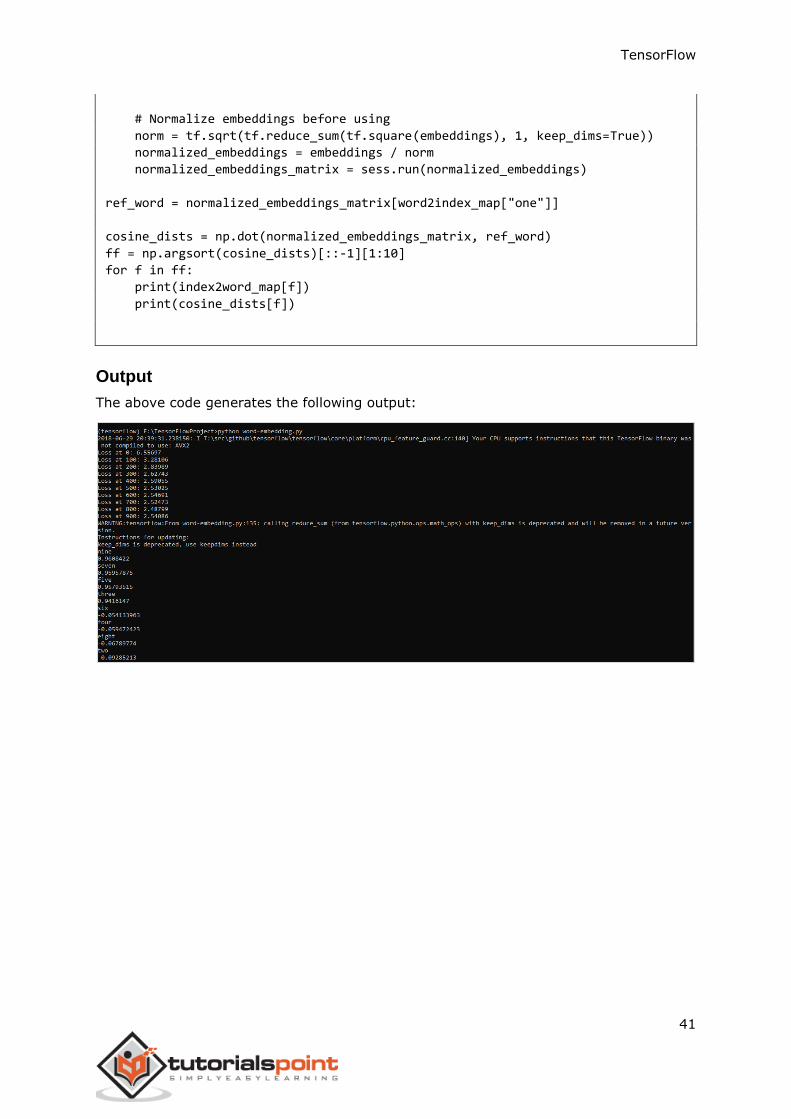
# Normalize embeddings before using

norm = tf.sqrt(tf.reduce_sum(tf.square(embeddings), 1, keep_dims=True))

normalized_embeddings = embeddings / norm

normalized_embeddings_matrix = sess.run(normalized_embeddings)

ref_word = normalized_embeddings_matrix[word2index_map["one"]]

cosine_dists = np.dot(normalized_embeddings_matrix, ref_word)

ff = np.argsort(cosine_dists)[::-1][1:10]

for f in ff:

print(index2word_map[f])

print(cosine_dists[f])

Output

The above code generates the following output:

TensorFlow

42

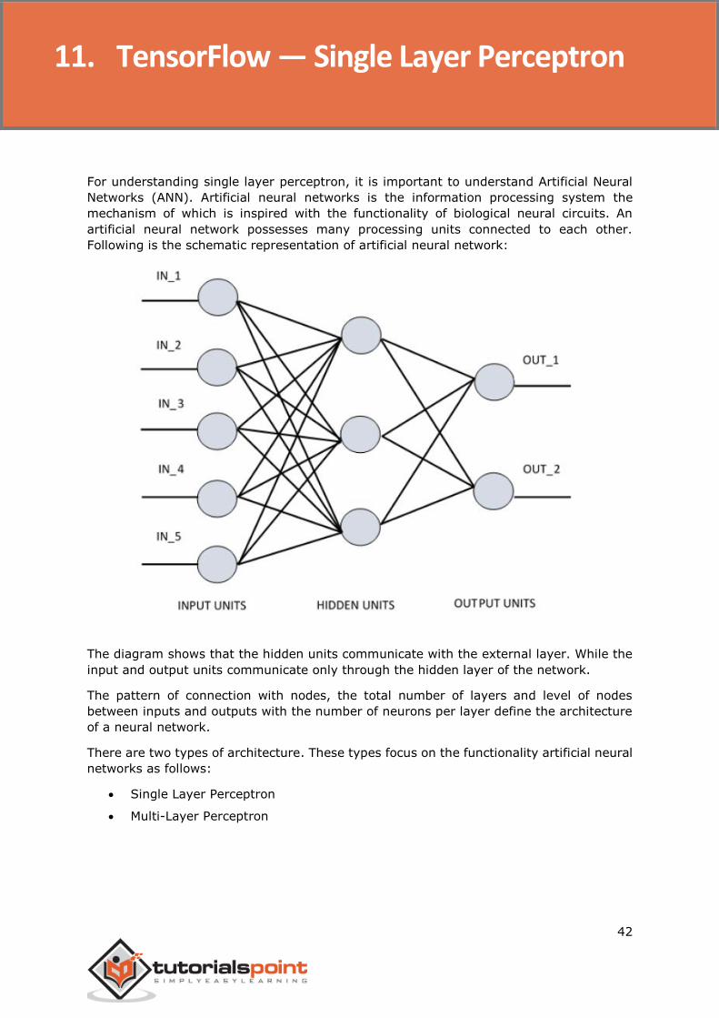
For understanding single layer perceptron, it is important to understand Artificial Neural

Networks (ANN). Artificial neural networks is the information processing system the

mechanism of which is inspired with the functionality of biological neural circuits. An

artificial neural network possesses many processing units connected to each other.

Following is the schematic representation of artificial neural network:

The diagram shows that the hidden units communicate with the external layer. While the

input and output units communicate only through the hidden layer of the network.

The pattern of connection with nodes, the total number of layers and level of nodes

between inputs and outputs with the number of neurons per layer define the architecture

of a neural network.

There are two types of architecture. These types focus on the functionality artificial neural

networks as follows:

Single Layer Perceptron

Multi-Layer Perceptron

11. TensorFlow — Single Layer Perceptron

TensorFlow

43

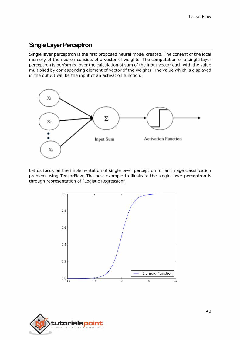
Single Layer Perceptron

Single layer perceptron is the first proposed neural model created. The content of the local

memory of the neuron consists of a vector of weights. The computation of a single layer

perceptron is performed over the calculation of sum of the input vector each with the value

multiplied by corresponding element of vector of the weights. The value which is displayed

in the output will be the input of an activation function.

Let us focus on the implementation of single layer perceptron for an image classification

problem using TensorFlow. The best example to illustrate the single layer perceptron is

through representation of “Logistic Regression”.

TensorFlow

44

Now, let us consider the following basic steps of training logistic regression:

The weights are initialized with random values at the beginning of the training.

For each element of the training set, the error is calculated with the difference

between desired output and the actual output. The error calculated is used to adjust

the weights.

The process is repeated until the error made on the entire training set is not less

than the specified threshold, until the maximum number of iterations is reached.

The complete code for evaluation of logistic regression is mentioned below:

# Import MINST data

from tensorflow.examples.tutorials.mnist import input_data

mnist = input_data.read_data_sets("/tmp/data/", one_hot=True)

import tensorflow as tf

import matplotlib.pyplot as plt

# Parameters

learning_rate = 0.01

training_epochs = 25

batch_size = 100

display_step = 1

# tf Graph Input

x = tf.placeholder("float", [None, 784]) # mnist data image of shape 28*28=784

y = tf.placeholder("float", [None, 10]) # 0-9 digits recognition => 10 classes

# Create model

# Set model weights

W = tf.Variable(tf.zeros([784, 10]))

b = tf.Variable(tf.zeros([10]))

# Construct model

activation = tf.nn.softmax(tf.matmul(x, W) + b) # Softmax

# Minimize error using cross entropy

cross_entropy = y*tf.log(activation)

cost = tf.reduce_mean\

(-tf.reduce_sum\

(cross_entropy,reduction_indices=1))

optimizer = tf.train.\

GradientDescentOptimizer(learning_rate).minimize(cost)

#Plot settings

avg_set = []

epoch_set=[]

# Initializing the variables

init = tf.initialize_all_variables()

TensorFlow

45

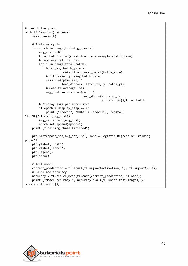
# Launch the graph

with tf.Session() as sess:

sess.run(init)

# Training cycle

for epoch in range(training_epochs):

avg_cost = 0.

total_batch = int(mnist.train.num_examples/batch_size)

# Loop over all batches

for i in range(total_batch):

batch_xs, batch_ys = \

mnist.train.next_batch(batch_size)

# Fit training using batch data

sess.run(optimizer, \

feed_dict={x: batch_xs, y: batch_ys})

# Compute average loss

avg_cost += sess.run(cost, \

feed_dict={x: batch_xs, \

y: batch_ys})/total_batch

# Display logs per epoch step

if epoch % display_step == 0:

print ("Epoch:", '%04d' % (epoch+1), "cost=",

"{:.9f}".format(avg_cost))

avg_set.append(avg_cost)

epoch_set.append(epoch+1)

print ("Training phase finished")

plt.plot(epoch_set,avg_set, 'o', label='Logistic Regression Training

phase')

plt.ylabel('cost')

plt.xlabel('epoch')

plt.legend()

plt.show()

# Test model

correct_prediction = tf.equal(tf.argmax(activation, 1), tf.argmax(y, 1))

# Calculate accuracy

accuracy = tf.reduce_mean(tf.cast(correct_prediction, "float"))

print ("Model accuracy:", accuracy.eval({x: mnist.test.images, y:

mnist.test.labels}))

TensorFlow

46

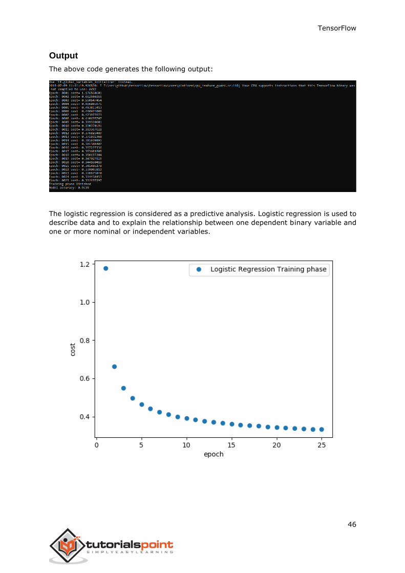
Output

The above code generates the following output:

The logistic regression is considered as a predictive analysis. Logistic regression is used to

describe data and to explain the relationship between one dependent binary variable and

one or more nominal or independent variables.

TensorFlow

47

In this chapter, we will focus on the basic example of linear regression implementation

using TensorFlow. Logistic regression or linear regression is a supervised machine learning

approach for the classification of order discrete categories. Our goal in this chapter is to

build a model by which a user can predict the relationship between predictor variables and

one or more independent variables.

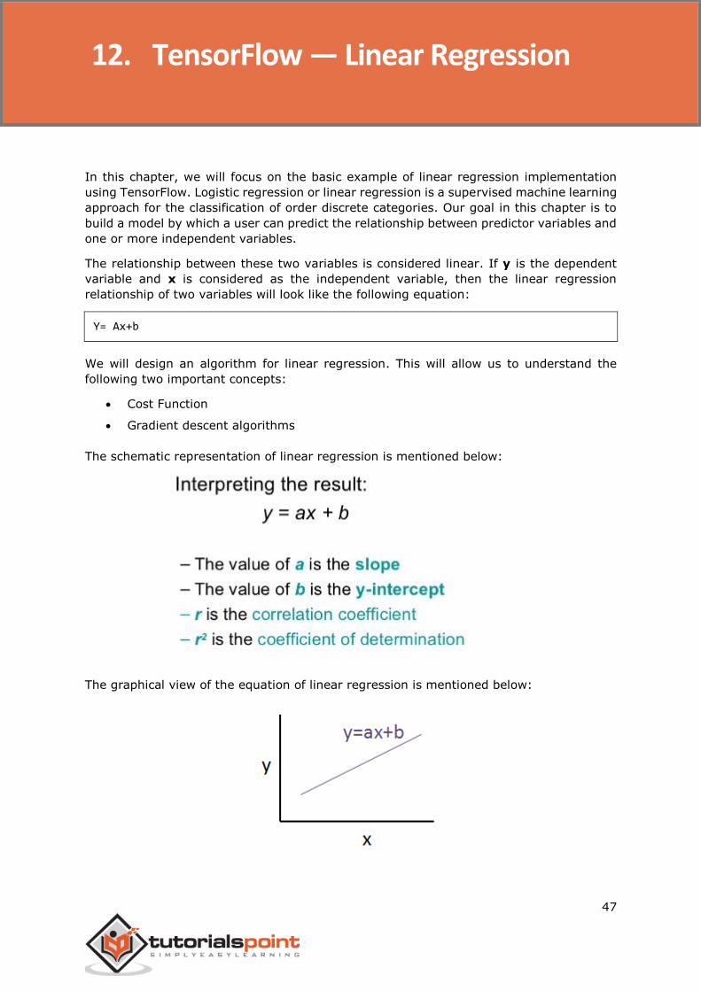
The relationship between these two variables is considered linear. If y is the dependent

variable and x is considered as the independent variable, then the linear regression

relationship of two variables will look like the following equation:

Y= Ax+b

We will design an algorithm for linear regression. This will allow us to understand the

following two important concepts:

Cost Function

Gradient descent algorithms

The schematic representation of linear regression is mentioned below:

The graphical view of the equation of linear regression is mentioned below:

12. TensorFlow — Linear Regression

TensorFlow

48

Steps to design an algorithm for linear regression

We will now learn about the steps that help in designing an algorithm for linear regression.

Step 1

It is important to import the necessary modules for plotting the linear regression module.

We start importing the Python library NumPy and Matplotlib.

import numpy as np

import matplotlib.pyplot as plt

Step 2

Define the number of coefficients necessary for logistic regression.

number_of_points = 500

x_point = []

y_point = []

a = 0.22

b = 0.78

Step 3

Iterate the variables for generating 300 random points around the regression equation:

Y=0.22x+0.78

for i in range(number_of_points):

x = np.random.normal(0.0,0.5)

y = a*x + b +np.random.normal(0.0,0.1)

x_point.append([x])

y_point.append([y])

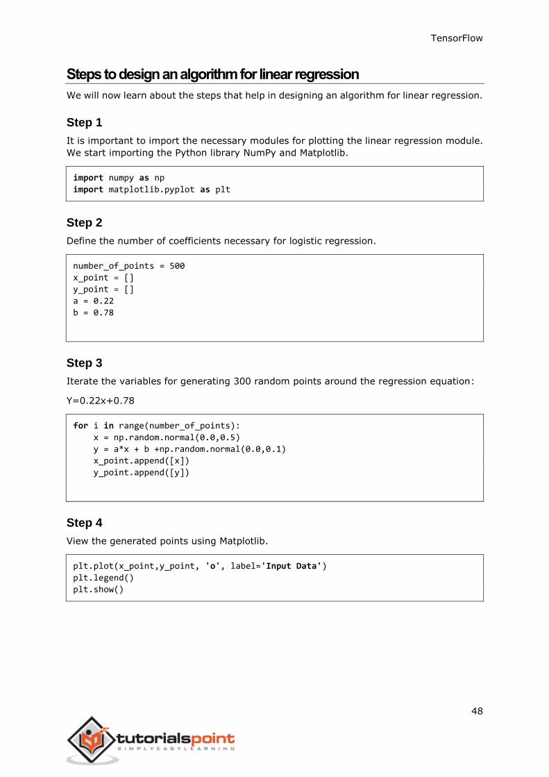
Step 4

View the generated points using Matplotlib.

plt.plot(x_point,y_point, 'o', label='Input Data')

plt.legend()

plt.show()

TensorFlow

49

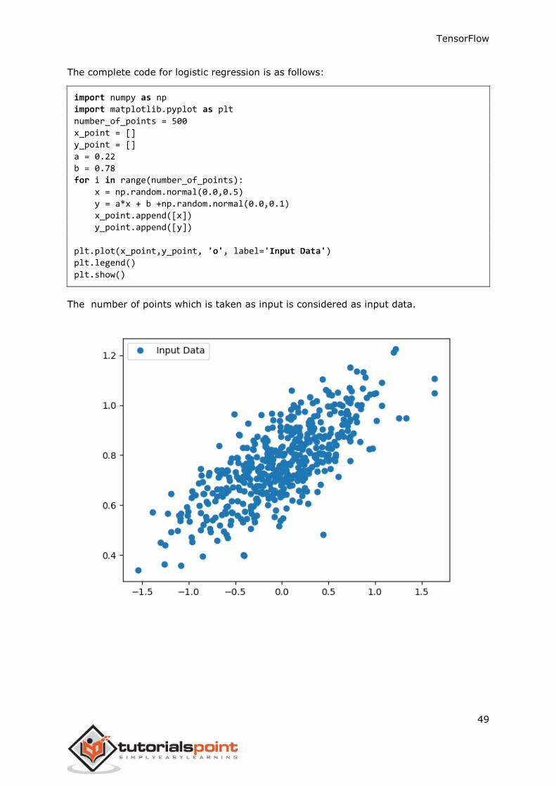
The complete code for logistic regression is as follows:

import numpy as np

import matplotlib.pyplot as plt

number_of_points = 500

x_point = []

y_point = []

a = 0.22

b = 0.78

for i in range(number_of_points):

x = np.random.normal(0.0,0.5)

y = a*x + b +np.random.normal(0.0,0.1)

x_point.append([x])

y_point.append([y])

plt.plot(x_point,y_point, 'o', label='Input Data')

plt.legend()

plt.show()

The number of points which is taken as input is considered as input data.

TensorFlow

50

TFLearn can be defined as a modular and transparent deep learning aspect used in

TensorFlow framework. The main motive of TFLearn is to provide a higher level API to

TensorFlow for facilitating and showing up new experiments.

Consider the following important features of TFLearn:

TFLearn is easy to use and understand.

It includes easy concepts to build highly modular network layers, optimizers and

various metrics embedded within them.

It includes full transparency with TensorFlow work system.

It includes powerful helper functions to train the built in tensors which accept

multiple inputs, outputs and optimizers.

It includes easy and beautiful graph visualization.

The graph visualization includes various details of weights, gradients and

activations.

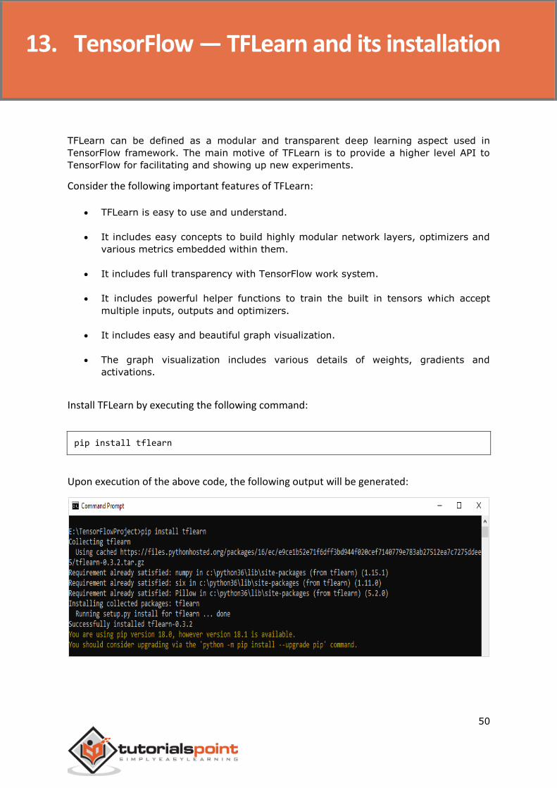
Install TFLearn by executing the following command:

pip install tflearn

Upon execution of the above code, the following output will be generated:

13. TensorFlow — TFLearn and its installation

TensorFlow

51

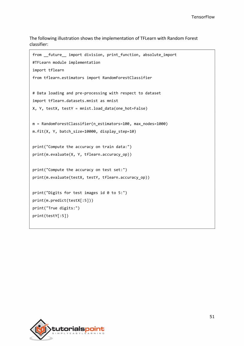
The following illustration shows the implementation of TFLearn with Random Forest classifier:

from __future__ import division, print_function, absolute_import

#TFLearn module implementation

import tflearn

from tflearn.estimators import RandomForestClassifier

# Data loading and pre-processing with respect to dataset

import tflearn.datasets.mnist as mnist

X, Y, testX, testY = mnist.load_data(one_hot=False)

m = RandomForestClassifier(n_estimators=100, max_nodes=1000)

m.fit(X, Y, batch_size=10000, display_step=10)

print("Compute the accuracy on train data:")

print(m.evaluate(X, Y, tflearn.accuracy_op))

print("Compute the accuracy on test set:")

print(m.evaluate(testX, testY, tflearn.accuracy_op))

print("Digits for test images id 0 to 5:")

print(m.predict(testX[:5]))

print("True digits:")

print(testY[:5])

TensorFlow

52

In this chapter, we will focus on the difference between CNN and RNN:

CNN RNN

It is suitable for spatial data such as

images.

RNN is suitable for temporal data, also

called sequential data.

CNN is considered to be more powerful

than RNN.

RNN includes less feature compatibility

when compared to CNN.

This network takes fixed size inputs and

generates fixed size outputs.

RNN can handle arbitrary input/output

lengths.

CNN is a type of feed-forward artificial

neural network with variations of

multilayer perceptrons designed to use

minimal amounts of preprocessing.

RNN unlike feed forward neural networks -

can use their internal memory to process

arbitrary sequences of inputs.

CNNs use connectivity pattern between the

neurons. This is inspired by the

organization of the animal visual cortex,

whose individual neurons are arranged in

such a way that they respond to

overlapping regions tiling the visual field.

Recurrent neural networks use time-series

information - what a user spoke last will

impact what he/she will speak next.

CNNs are ideal for images and video

processing.

RNNs are ideal for text and speech

analysis.

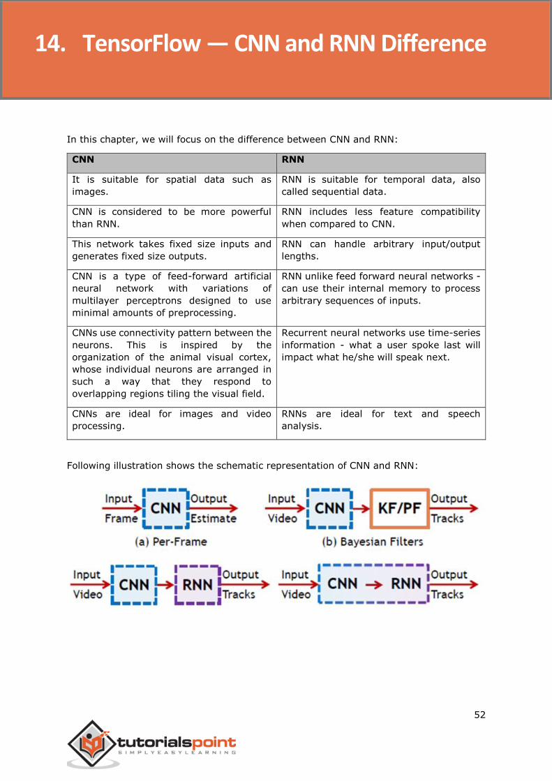
Following illustration shows the schematic representation of CNN and RNN:

14. TensorFlow — CNN and RNN Difference

TensorFlow

53

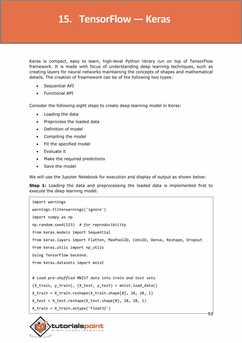
Keras is compact, easy to learn, high-level Python library run on top of TensorFlow

framework. It is made with focus of understanding deep learning techniques, such as

creating layers for neural networks maintaining the concepts of shapes and mathematical

details. The creation of freamework can be of the following two types:

Sequential API

Functional API

Consider the following eight steps to create deep learning model in Keras:

Loading the data

Preprocess the loaded data

Definition of model

Compiling the model

Fit the specified model

Evaluate it

Make the required predictions

Save the model

We will use the Jupyter Notebook for execution and display of output as shown below:

Step 1: Loading the data and preprocessing the loaded data is implemented first to

execute the deep learning model.

import warnings

warnings.filterwarnings('ignore')

import numpy as np

np.random.seed(123) # for reproducibility

from keras.models import Sequential

from keras.layers import Flatten, MaxPool2D, Conv2D, Dense, Reshape, Dropout

from keras.utils import np_utils

Using TensorFlow backend.

from keras.datasets import mnist

# Load pre-shuffled MNIST data into train and test sets

(X_train, y_train), (X_test, y_test) = mnist.load_data()

X_train = X_train.reshape(X_train.shape[0], 28, 28, 1)

X_test = X_test.reshape(X_test.shape[0], 28, 28, 1)

X_train = X_train.astype('float32')

15. TensorFlow — Keras

TensorFlow

54

X_test = X_test.astype('float32')

X_train /= 255

X_test /= 255

Y_train = np_utils.to_categorical(y_train, 10)

Y_test = np_utils.to_categorical(y_test, 10)

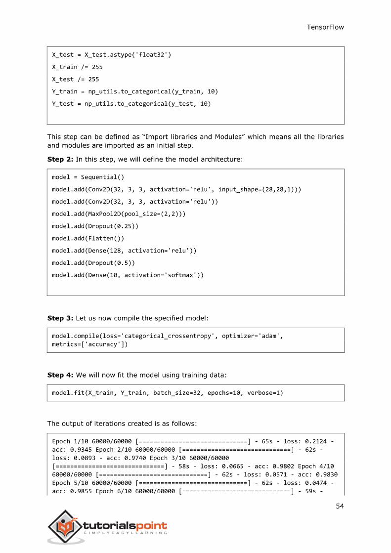
This step can be defined as “Import libraries and Modules” which means all the libraries

and modules are imported as an initial step.

Step 2: In this step, we will define the model architecture:

model = Sequential()

model.add(Conv2D(32, 3, 3, activation='relu', input_shape=(28,28,1)))

model.add(Conv2D(32, 3, 3, activation='relu'))

model.add(MaxPool2D(pool_size=(2,2)))

model.add(Dropout(0.25))

model.add(Flatten())

model.add(Dense(128, activation='relu'))

model.add(Dropout(0.5))

model.add(Dense(10, activation='softmax'))

Step 3: Let us now compile the specified model:

model.compile(loss='categorical_crossentropy', optimizer='adam',

metrics=['accuracy'])

Step 4: We will now fit the model using training data:

model.fit(X_train, Y_train, batch_size=32, epochs=10, verbose=1)

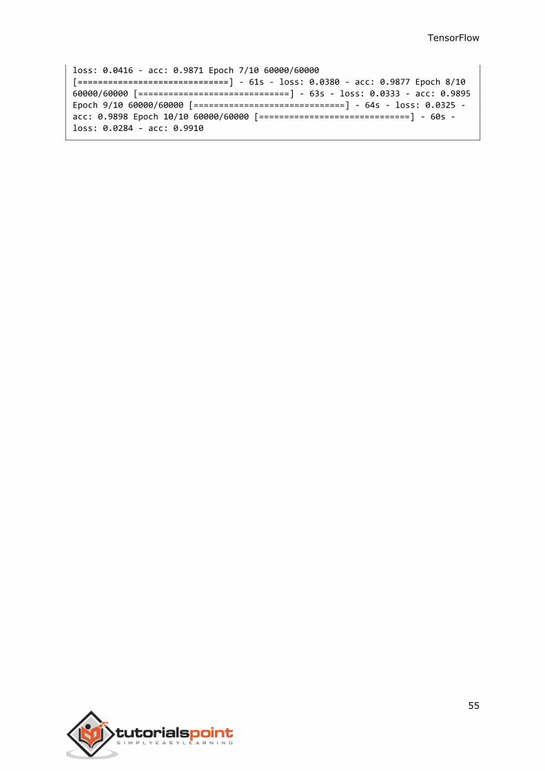
The output of iterations created is as follows:

Epoch 1/10 60000/60000 [==============================] - 65s - loss: 0.2124 -

acc: 0.9345 Epoch 2/10 60000/60000 [==============================] - 62s -

loss: 0.0893 - acc: 0.9740 Epoch 3/10 60000/60000

[==============================] - 58s - loss: 0.0665 - acc: 0.9802 Epoch 4/10

60000/60000 [==============================] - 62s - loss: 0.0571 - acc: 0.9830

Epoch 5/10 60000/60000 [==============================] - 62s - loss: 0.0474 -

acc: 0.9855 Epoch 6/10 60000/60000 [==============================] - 59s -

TensorFlow

55

loss: 0.0416 - acc: 0.9871 Epoch 7/10 60000/60000

[==============================] - 61s - loss: 0.0380 - acc: 0.9877 Epoch 8/10

60000/60000 [==============================] - 63s - loss: 0.0333 - acc: 0.9895

Epoch 9/10 60000/60000 [==============================] - 64s - loss: 0.0325 -

acc: 0.9898 Epoch 10/10 60000/60000 [==============================] - 60s -

loss: 0.0284 - acc: 0.9910

TensorFlow

56

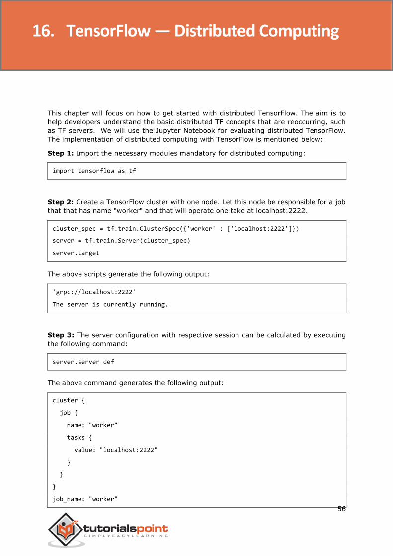
This chapter will focus on how to get started with distributed TensorFlow. The aim is to

help developers understand the basic distributed TF concepts that are reoccurring, such

as TF servers. We will use the Jupyter Notebook for evaluating distributed TensorFlow.

The implementation of distributed computing with TensorFlow is mentioned below:

Step 1: Import the necessary modules mandatory for distributed computing:

import tensorflow as tf

Step 2: Create a TensorFlow cluster with one node. Let this node be responsible for a job

that that has name "worker" and that will operate one take at localhost:2222.

cluster_spec = tf.train.ClusterSpec({'worker' : ['localhost:2222']})

server = tf.train.Server(cluster_spec)

server.target

The above scripts generate the following output:

'grpc://localhost:2222'

The server is currently running.

Step 3: The server configuration with respective session can be calculated by executing

the following command:

server.server_def

The above command generates the following output:

cluster {

job {

name: "worker"

tasks {

value: "localhost:2222"

}

}

}

job_name: "worker"

16. TensorFlow — Distributed Computing

TensorFlow

57

protocol: "grpc"

Step 4: Launch a TensorFlow session with the execution engine being the server. Use

TensorFlow to create a local server and use lsof to find out the location of the server.

sess = tf.Session(target=server.target)

server = tf.train.Server.create_local_server()

Step 5: View devices available in this session and close the respective session.

devices = sess.list_devices()

for d in devices:

print(d.name)

sess.close()

The above command generates the following output:

/job:worker/replica:0/task:0/device:CPU:0

TensorFlow

58

Here, we will focus on MetaGraph formation in TensorFlow. This will help us understand

export module in TensorFlow. The MetaGraph contains the basic information, which is

required to train, perform evaluation, or run inference on a previously trained graph.

Following is the code snippet for the same:

def export_meta_graph(filename=None, collection_list=None, as_text=False):

"""this code writes `MetaGraphDef` to save_path/filename.

Arguments:

filename: Optional meta_graph filename including the path.

collection_list: List of string keys to collect.

as_text: If `True`, writes the meta_graph as an ASCII proto.

Returns:

A `MetaGraphDef` proto.

"""

One of the typical usage model for the same is mentioned below:

# Build the model

...

with tf.Session() as sess:

# Use the model

...

# Export the model to /tmp/my-model.meta.

meta_graph_def = tf.train.export_meta_graph(filename='/tmp/my-model.meta')

17. TensorFlow — Exporting with TensorFlow

TensorFlow

59

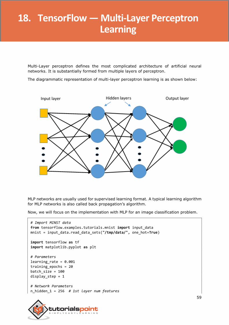
Multi-Layer perceptron defines the most complicated architecture of artificial neural

networks. It is substantially formed from multiple layers of perceptron.

The diagrammatic representation of multi-layer perceptron learning is as shown below:

MLP networks are usually used for supervised learning format. A typical learning algorithm

for MLP networks is also called back propagation’s algorithm.

Now, we will focus on the implementation with MLP for an image classification problem.

# Import MINST data

from tensorflow.examples.tutorials.mnist import input_data

mnist = input_data.read_data_sets("/tmp/data/", one_hot=True)

import tensorflow as tf

import matplotlib.pyplot as plt

# Parameters

learning_rate = 0.001

training_epochs = 20

batch_size = 100

display_step = 1

# Network Parameters

n_hidden_1 = 256 # 1st layer num features

18. TensorFlow — Multi-Layer Perceptron Learning

TensorFlow

60

n_hidden_2 = 256 # 2nd layer num features

n_input = 784 # MNIST data input (img shape: 28*28)

n_classes = 10 # MNIST total classes (0-9 digits)

# tf Graph input

x = tf.placeholder("float", [None, n_input])

y = tf.placeholder("float", [None, n_classes])

# weights layer 1

h = tf.Variable(tf.random_normal([n_input, n_hidden_1]))

# bias layer 1

bias_layer_1 = tf.Variable(tf.random_normal([n_hidden_1]))

# layer 1

layer_1 = tf.nn.sigmoid(tf.add(tf.matmul(x, h), bias_layer_1))

# weights layer 2

w = tf.Variable(tf.random_normal([n_hidden_1, n_hidden_2]))

# bias layer 2

bias_layer_2 = tf.Variable(tf.random_normal([n_hidden_2]))

# layer 2

layer_2 = tf.nn.sigmoid(tf.add(tf.matmul(layer_1, w), bias_layer_2))

# weights output layer

output = tf.Variable(tf.random_normal([n_hidden_2, n_classes]))

# biar output layer

bias_output = tf.Variable(tf.random_normal([n_classes]))

# output layer

output_layer = tf.matmul(layer_2, output) + bias_output

# cost function

cost =

tf.reduce_mean(tf.nn.sigmoid_cross_entropy_with_logits(logits=output_layer,

labels=y))

#cost = tf.reduce_mean(tf.nn.sigmoid_cross_entropy_with_logits(output_layer,

y))

# optimizer

optimizer = tf.train.AdamOptimizer(learning_rate=learning_rate).minimize(cost)

# optimizer =

tf.train.GradientDescentOptimizer(learning_rate=learning_rate).minimize(cost)

# Plot settings

avg_set = []

epoch_set = []

# Initializing the variables

init = tf.global_variables_initializer()

# Launch the graph

with tf.Session() as sess:

sess.run(init)

# Training cycle

TensorFlow

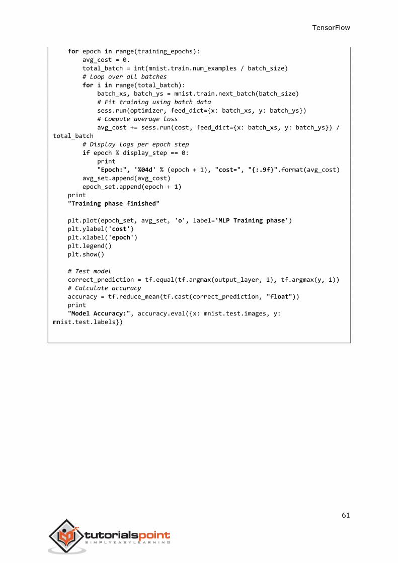
61

for epoch in range(training_epochs):

avg_cost = 0.

total_batch = int(mnist.train.num_examples / batch_size)

# Loop over all batches

for i in range(total_batch):

batch_xs, batch_ys = mnist.train.next_batch(batch_size)

# Fit training using batch data

sess.run(optimizer, feed_dict={x: batch_xs, y: batch_ys})

# Compute average loss

avg_cost += sess.run(cost, feed_dict={x: batch_xs, y: batch_ys}) /

total_batch

# Display logs per epoch step

if epoch % display_step == 0:

print

"Epoch:", '%04d' % (epoch + 1), "cost=", "{:.9f}".format(avg_cost)

avg_set.append(avg_cost)

epoch_set.append(epoch + 1)

print

"Training phase finished"

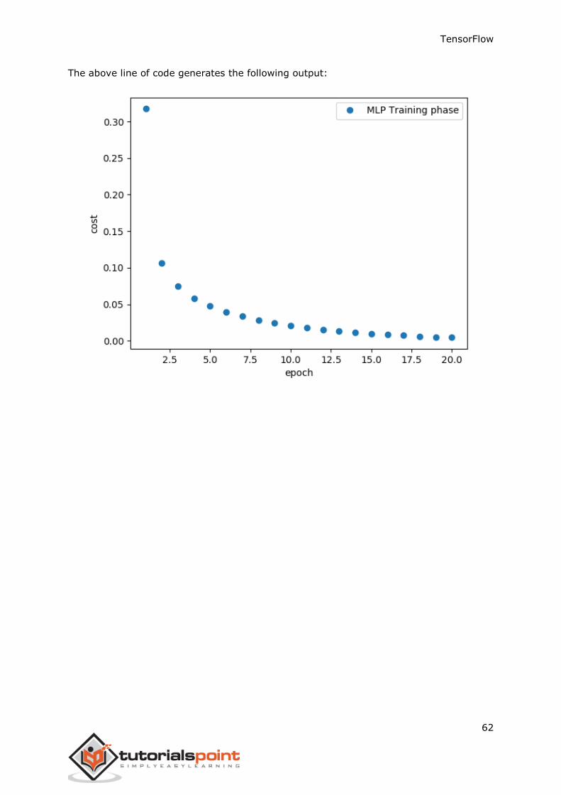
plt.plot(epoch_set, avg_set, 'o', label='MLP Training phase')

plt.ylabel('cost')

plt.xlabel('epoch')

plt.legend()

plt.show()

# Test model

correct_prediction = tf.equal(tf.argmax(output_layer, 1), tf.argmax(y, 1))

# Calculate accuracy

accuracy = tf.reduce_mean(tf.cast(correct_prediction, "float"))

print

"Model Accuracy:", accuracy.eval({x: mnist.test.images, y:

mnist.test.labels})

TensorFlow

62

The above line of code generates the following output:

TensorFlow

63

In this chapter, we will be focus on the network we will have to learn from known set of

points called x and f(x). A single hidden layer will build this simple network.

The code for the explanation of hidden layers of perceptron is as shown below:

#Importing the necessary modules

import tensorflow as tf

import numpy as np

import math, random

import matplotlib.pyplot as plt

np.random.seed(1000)

function_to_learn = lambda x: np.cos(x) + 0.1*np.random.randn(*x.shape)

layer_1_neurons = 10

NUM_points = 1000

#Training the parameters

batch_size = 100

NUM_EPOCHS = 1500

all_x = np.float32(np.random.uniform(-2*math.pi, 2*math.pi, (1, NUM_points))).T

np.random.shuffle(all_x)

train_size = int(900)

#Training the first 700 points in the given set

x_training = all_x[:train_size]

y_training = function_to_learn(x_training)

#Training the last 300 points in the given set

x_validation = all_x[train_size:]

y_validation = function_to_learn(x_validation)

plt.figure(1)

plt.scatter(x_training, y_training, c='blue', label='train')

plt.scatter(x_validation, y_validation, c='pink', label='validation')

plt.legend()

plt.show()

X = tf.placeholder(tf.float32, [None, 1], name="X")

Y = tf.placeholder(tf.float32, [None, 1], name="Y")

#first layer

#Number of neurons = 10

w_h = tf.Variable(tf.random_uniform([1, layer_1_neurons],\

minval=-1, maxval=1, dtype=tf.float32))

b_h = tf.Variable(tf.zeros([1, layer_1_neurons], dtype=tf.float32))

h = tf.nn.sigmoid(tf.matmul(X, w_h) + b_h)

19. TensorFlow — Hidden Layers of Perceptron

TensorFlow

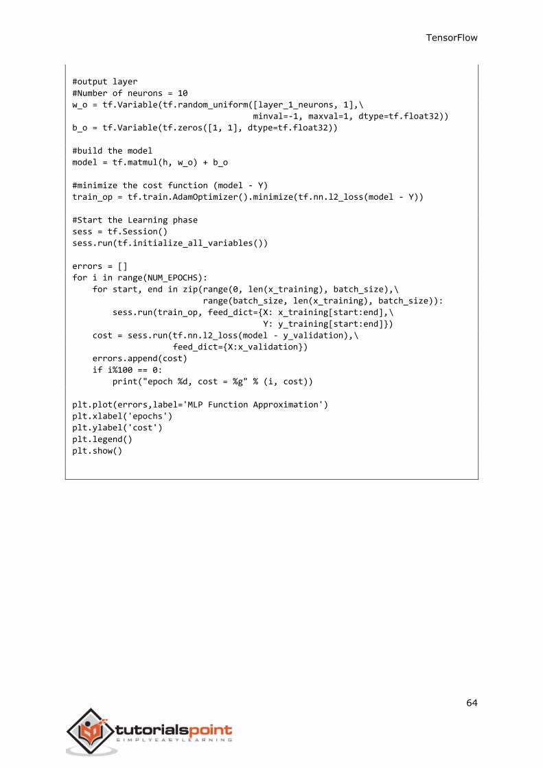
64

#output layer

#Number of neurons = 10

w_o = tf.Variable(tf.random_uniform([layer_1_neurons, 1],\

minval=-1, maxval=1, dtype=tf.float32))

b_o = tf.Variable(tf.zeros([1, 1], dtype=tf.float32))

#build the model

model = tf.matmul(h, w_o) + b_o

#minimize the cost function (model - Y)

train_op = tf.train.AdamOptimizer().minimize(tf.nn.l2_loss(model - Y))

#Start the Learning phase

sess = tf.Session()

sess.run(tf.initialize_all_variables())

errors = []

for i in range(NUM_EPOCHS):

for start, end in zip(range(0, len(x_training), batch_size),\

range(batch_size, len(x_training), batch_size)):

sess.run(train_op, feed_dict={X: x_training[start:end],\

Y: y_training[start:end]})

cost = sess.run(tf.nn.l2_loss(model - y_validation),\

feed_dict={X:x_validation})

errors.append(cost)

if i%100 == 0:

print("epoch %d, cost = %g" % (i, cost))

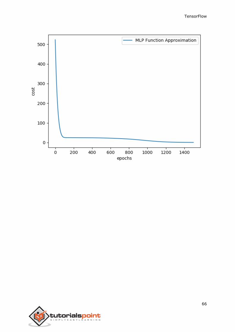
plt.plot(errors,label='MLP Function Approximation')

plt.xlabel('epochs')

plt.ylabel('cost')

plt.legend()

plt.show()

TensorFlow

65

Output

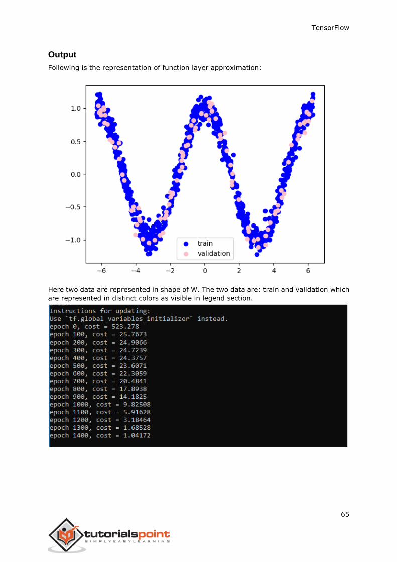
Following is the representation of function layer approximation:

Here two data are represented in shape of W. The two data are: train and validation which

are represented in distinct colors as visible in legend section.

TensorFlow

66

TensorFlow

67

Optimizers are the extended class, which include added information to train a specific

model. The optimizer class is initialized with given parameters but it is important to

remember that no Tensor is needed. The optimizers are used for improving speed and

performance for training a specific model.

The basic optimizer of TensorFlow is:

tf.train.Optimizer

This class is defined in the specified path of “tensorflow/python/training/optimizer.py”.

Following are some optimizers in Tensorflow:

Stochastic Gradient descent

Stochastic Gradient descent with gradient clipping

Momentum

Nesterov momentum

Adagrad

Adadelta

RMSProp

Adam

Adamax

SMORMS3

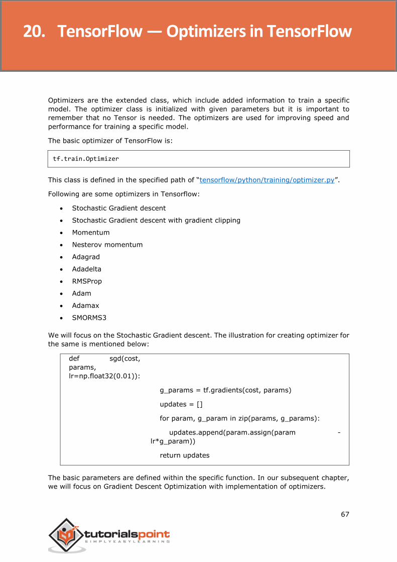
We will focus on the Stochastic Gradient descent. The illustration for creating optimizer for

the same is mentioned below:

def sgd(cost,

params,

lr=np.float32(0.01)):

g_params = tf.gradients(cost, params)

updates = []

for param, g_param in zip(params, g_params):

updates.append(param.assign(param -

lr*g_param))

return updates

The basic parameters are defined within the specific function. In our subsequent chapter,

we will focus on Gradient Descent Optimization with implementation of optimizers.

20. TensorFlow — Optimizers in TensorFlow

TensorFlow

68

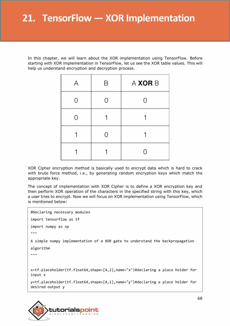
In this chapter, we will learn about the XOR implementation using TensorFlow. Before

starting with XOR implementation in TensorFlow, let us see the XOR table values. This will

help us understand encryption and decryption process.

XOR Cipher encryption method is basically used to encrypt data which is hard to crack

with brute force method, i.e., by generating random encryption keys which match the

appropriate key.

The concept of implementation with XOR Cipher is to define a XOR encryption key and

then perform XOR operation of the characters in the specified string with this key, which

a user tries to encrypt. Now we will focus on XOR implementation using TensorFlow, which

is mentioned below:

#Declaring necessary modules

import tensorflow as tf

import numpy as np

"""

A simple numpy implementation of a XOR gate to understand the backpropagation

algorithm

"""

x=tf.placeholder(tf.float64,shape=[4,2],name="x")#declaring a place holder for

input x

y=tf.placeholder(tf.float64,shape=[4,1],name="y")#declaring a place holder for

desired output y

21. TensorFlow — XOR Implementation

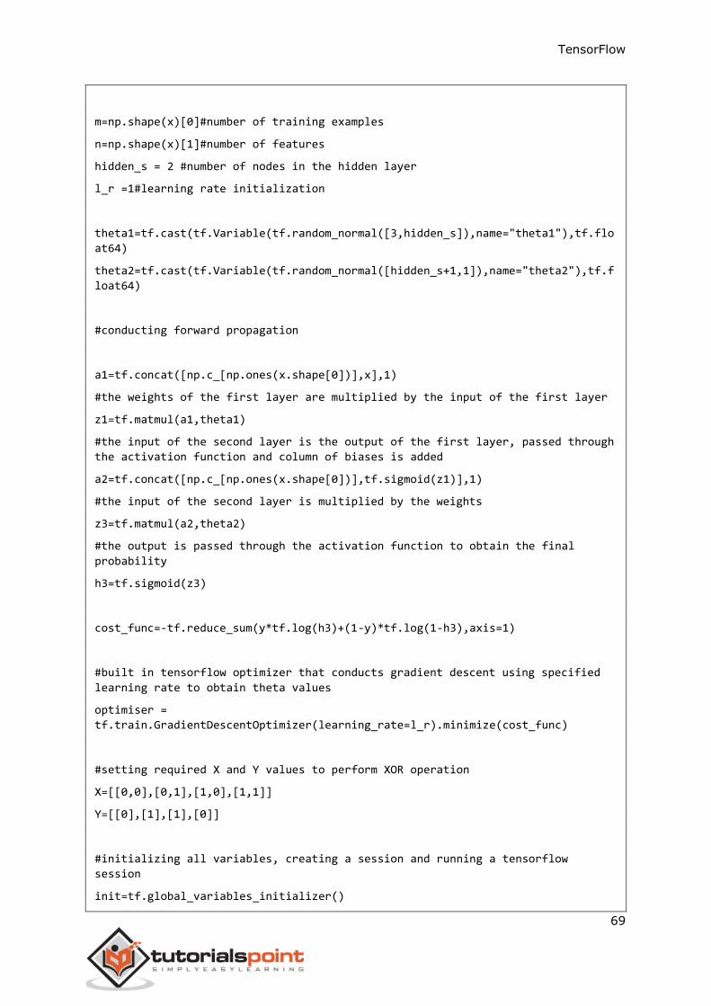
TensorFlow

69

m=np.shape(x)[0]#number of training examples

n=np.shape(x)[1]#number of features

hidden_s = 2 #number of nodes in the hidden layer

l_r =1#learning rate initialization

theta1=tf.cast(tf.Variable(tf.random_normal([3,hidden_s]),name="theta1"),tf.flo

at64)

theta2=tf.cast(tf.Variable(tf.random_normal([hidden_s+1,1]),name="theta2"),tf.f

loat64)

#conducting forward propagation

a1=tf.concat([np.c_[np.ones(x.shape[0])],x],1)

#the weights of the first layer are multiplied by the input of the first layer

z1=tf.matmul(a1,theta1)

#the input of the second layer is the output of the first layer, passed through

the activation function and column of biases is added

a2=tf.concat([np.c_[np.ones(x.shape[0])],tf.sigmoid(z1)],1)

#the input of the second layer is multiplied by the weights

z3=tf.matmul(a2,theta2)

#the output is passed through the activation function to obtain the final

probability

h3=tf.sigmoid(z3)

cost_func=-tf.reduce_sum(y*tf.log(h3)+(1-y)*tf.log(1-h3),axis=1)

#built in tensorflow optimizer that conducts gradient descent using specified

learning rate to obtain theta values

optimiser =

tf.train.GradientDescentOptimizer(learning_rate=l_r).minimize(cost_func)

#setting required X and Y values to perform XOR operation

X=[[0,0],[0,1],[1,0],[1,1]]

Y=[[0],[1],[1],[0]]

#initializing all variables, creating a session and running a tensorflow

session

init=tf.global_variables_initializer()

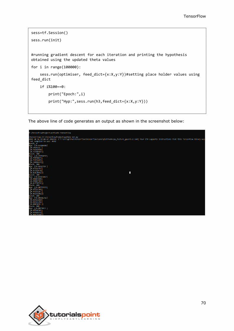
TensorFlow

70

sess=tf.Session()

sess.run(init)

#running gradient descent for each iteration and printing the hypothesis

obtained using the updated theta values

for i in range(100000):

sess.run(optimiser, feed_dict={x:X,y:Y})#setting place holder values using

feed_dict

if i%100==0:

print("Epoch:",i)

print("Hyp:",sess.run(h3,feed_dict={x:X,y:Y}))

The above line of code generates an output as shown in the screenshot below:

TensorFlow

71

Gradient descent optimization is considered to be an important concept in data science.

Consider the steps shown below to understand the implementation of gradient descent

optimization:

Step 1

Include necessary modules and declaration of x and y variables through which we are

going to define the gradient descent optimization.

import tensorflow as tf

x = tf.Variable(2, name='x', dtype=tf.float32)

log_x = tf.log(x)

log_x_squared = tf.square(log_x)

optimizer = tf.train.GradientDescentOptimizer(0.5)

train = optimizer.minimize(log_x_squared)

Step 2

Initialize the necessary variables and call the optimizers for defining and calling it with

respective function.

init = tf.initialize_all_variables()

def optimize():

with tf.Session() as session:

session.run(init)

print("starting at", "x:", session.run(x), "log(x)^2:",

session.run(log_x_squared))

for step in range(10):

session.run(train)

print("step", step, "x:", session.run(x), "log(x)^2:",

session.run(log_x_squared))

22. TensorFlow — Gradient Descent Optimization

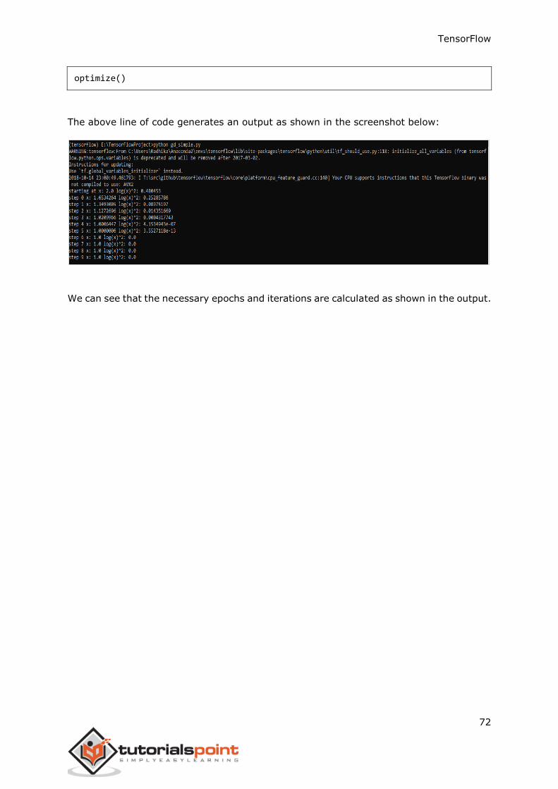
TensorFlow

72

optimize()

The above line of code generates an output as shown in the screenshot below:

We can see that the necessary epochs and iterations are calculated as shown in the output.

TensorFlow

73

A partial differential equation (PDE) is a differential equation, which involves partial

derivatives with unknown function of several independent variables. With reference to

partial differential equations, we will focus on creating new graphs.

Let us assume there is a pond with dimension 500*500 square:

N=500

Now, we will compute partial differential equation and form the respective graph using it.

Consider the steps given below for computing graph.

Step 1: Import libraries for simulation.

import tensorflow as tf

import numpy as np

import matplotlib.pyplot as plt

Step 2: Include functions for transformation of a 2D array into a convolution kernel and

simplified 2D convolution operation.

def make_kernel(a):

a = np.asarray(a)

a = a.reshape(list(a.shape) + [1,1])

return tf.constant(a, dtype=1)

def simple_conv(x, k):

"""A simplified 2D convolution operation"""

x = tf.expand_dims(tf.expand_dims(x, 0), -1)

y = tf.nn.depthwise_conv2d(x, k, [1, 1, 1, 1], padding='SAME')

return y[0, :, :, 0]

def laplace(x):

"""Compute the 2D laplacian of an array"""

laplace_k = make_kernel([[0.5, 1.0, 0.5],

[1.0, -6., 1.0],

[0.5, 1.0, 0.5]])

return simple_conv(x, laplace_k)

23. TensorFlow — Forming Graphs

TensorFlow

74

sess = tf.InteractiveSession()

Step 3: Include the number of iterations and compute the graph to display the records

accordingly.

N = 500

# Initial Conditions -- some rain drops hit a pond

# Set everything to zero

u_init = np.zeros([N, N], dtype=np.float32)

ut_init = np.zeros([N, N], dtype=np.float32)

# Some rain drops hit a pond at random points

for n in range(100):

a,b = np.random.randint(0, N, 2)

u_init[a,b] = np.random.uniform()

plt.imshow(u_init)

plt.show()

# Parameters:

# eps -- time resolution

# damping -- wave damping

eps = tf.placeholder(tf.float32, shape=())

damping = tf.placeholder(tf.float32, shape=())

# Create variables for simulation state

U = tf.Variable(u_init)

Ut = tf.Variable(ut_init)

# Discretized PDE update rules

U_ = U + eps * Ut

Ut_ = Ut + eps * (laplace(U) - damping * Ut)

# Operation to update the state

TensorFlow

75

step = tf.group(

U.assign(U_),

Ut.assign(Ut_))

# Initialize state to initial conditions

tf.initialize_all_variables().run()

# Run 1000 steps of PDE

for i in range(1000):

# Step simulation

step.run({eps: 0.03, damping: 0.04})

# Visualize every 50 steps

if i % 500 == 0:

plt.imshow(U.eval())

plt.show()

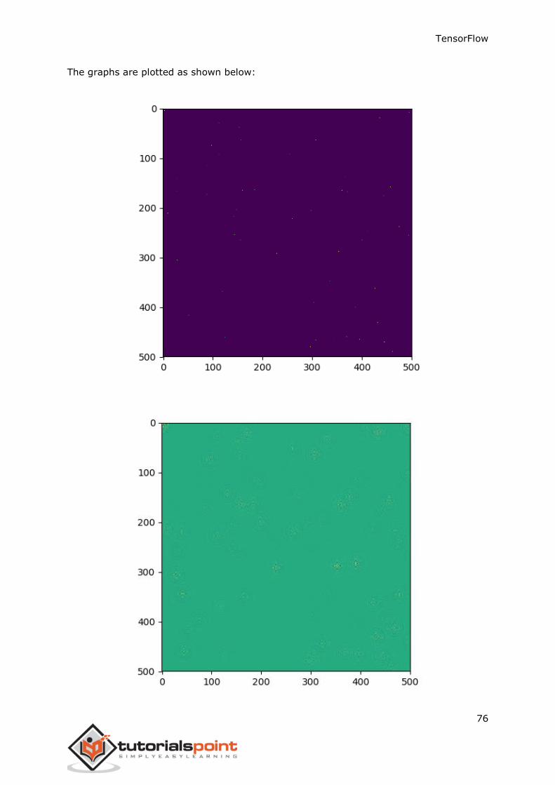
TensorFlow

76

The graphs are plotted as shown below:

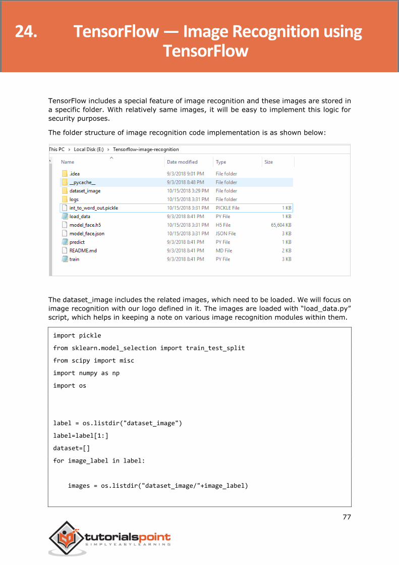
TensorFlow

77

TensorFlow includes a special feature of image recognition and these images are stored in

a specific folder. With relatively same images, it will be easy to implement this logic for

security purposes.

The folder structure of image recognition code implementation is as shown below:

The dataset_image includes the related images, which need to be loaded. We will focus on

image recognition with our logo defined in it. The images are loaded with “load_data.py”

script, which helps in keeping a note on various image recognition modules within them.

import pickle

from sklearn.model_selection import train_test_split

from scipy import misc

import numpy as np

import os

label = os.listdir("dataset_image")

label=label[1:]

dataset=[]

for image_label in label:

images = os.listdir("dataset_image/"+image_label)

24. TensorFlow — Image Recognition using TensorFlow

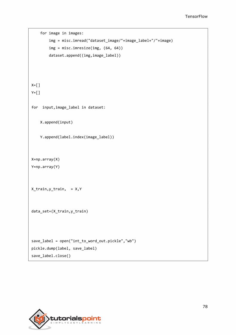
TensorFlow

78

for image in images:

img = misc.imread("dataset_image/"+image_label+"/"+image)

img = misc.imresize(img, (64, 64))

dataset.append((img,image_label))

X=[]

Y=[]

for input,image_label in dataset:

X.append(input)

Y.append(label.index(image_label))

X=np.array(X)

Y=np.array(Y)

X_train,y_train, = X,Y

data_set=(X_train,y_train)

save_label = open("int_to_word_out.pickle","wb")

pickle.dump(label, save_label)

save_label.close()

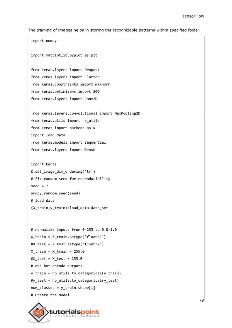
TensorFlow

79

The training of images helps in storing the recognizable patterns within specified folder.

import numpy

import matplotlib.pyplot as plt

from keras.layers import Dropout

from keras.layers import Flatten

from keras.constraints import maxnorm

from keras.optimizers import SGD

from keras.layers import Conv2D

from keras.layers.convolutional import MaxPooling2D

from keras.utils import np_utils

from keras import backend as K

import load_data

from keras.models import Sequential

from keras.layers import Dense

import keras

K.set_image_dim_ordering('tf')

# fix random seed for reproducibility

seed = 7

numpy.random.seed(seed)

# load data

(X_train,y_train)=load_data.data_set

# normalize inputs from 0-255 to 0.0-1.0

X_train = X_train.astype('float32')

#X_test = X_test.astype('float32')

X_train = X_train / 255.0

#X_test = X_test / 255.0

# one hot encode outputs

y_train = np_utils.to_categorical(y_train)

#y_test = np_utils.to_categorical(y_test)

num_classes = y_train.shape[1]

# Create the model

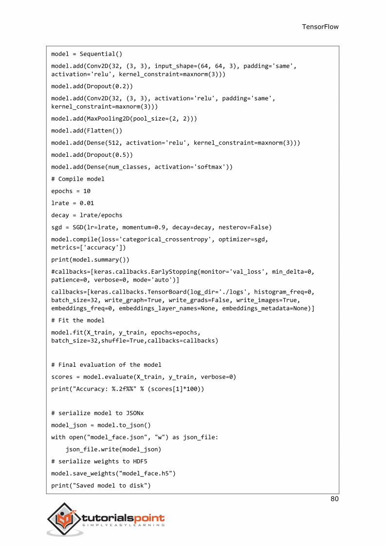
TensorFlow

80

model = Sequential()

model.add(Conv2D(32, (3, 3), input_shape=(64, 64, 3), padding='same',

activation='relu', kernel_constraint=maxnorm(3)))

model.add(Dropout(0.2))

model.add(Conv2D(32, (3, 3), activation='relu', padding='same',

kernel_constraint=maxnorm(3)))

model.add(MaxPooling2D(pool_size=(2, 2)))

model.add(Flatten())

model.add(Dense(512, activation='relu', kernel_constraint=maxnorm(3)))

model.add(Dropout(0.5))

model.add(Dense(num_classes, activation='softmax'))

# Compile model

epochs = 10

lrate = 0.01

decay = lrate/epochs

sgd = SGD(lr=lrate, momentum=0.9, decay=decay, nesterov=False)

model.compile(loss='categorical_crossentropy', optimizer=sgd,

metrics=['accuracy'])

print(model.summary())

#callbacks=[keras.callbacks.EarlyStopping(monitor='val_loss', min_delta=0,

patience=0, verbose=0, mode='auto')]

callbacks=[keras.callbacks.TensorBoard(log_dir='./logs', histogram_freq=0,

batch_size=32, write_graph=True, write_grads=False, write_images=True,

embeddings_freq=0, embeddings_layer_names=None, embeddings_metadata=None)]

# Fit the model

model.fit(X_train, y_train, epochs=epochs,

batch_size=32,shuffle=True,callbacks=callbacks)

# Final evaluation of the model

scores = model.evaluate(X_train, y_train, verbose=0)

print("Accuracy: %.2f%%" % (scores[1]*100))

# serialize model to JSONx

model_json = model.to_json()

with open("model_face.json", "w") as json_file:

json_file.write(model_json)

# serialize weights to HDF5

model.save_weights("model_face.h5")

print("Saved model to disk")

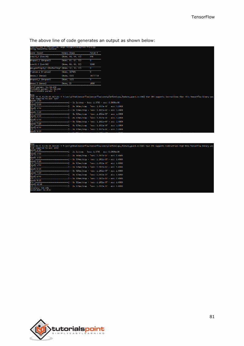
TensorFlow

81

The above line of code generates an output as shown below:

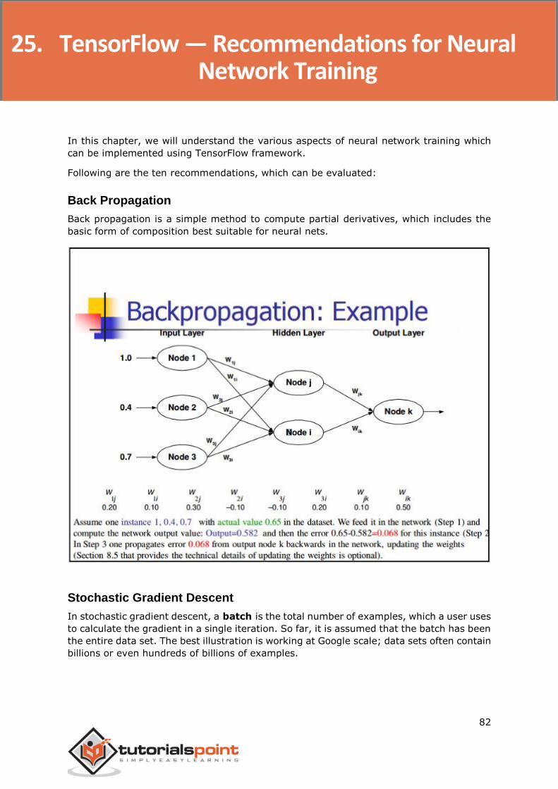
TensorFlow

82

In this chapter, we will understand the various aspects of neural network training which

can be implemented using TensorFlow framework.

Following are the ten recommendations, which can be evaluated:

Back Propagation

Back propagation is a simple method to compute partial derivatives, which includes the

basic form of composition best suitable for neural nets.

Stochastic Gradient Descent

In stochastic gradient descent, a batch is the total number of examples, which a user uses

to calculate the gradient in a single iteration. So far, it is assumed that the batch has been

the entire data set. The best illustration is working at Google scale; data sets often contain

billions or even hundreds of billions of examples.

25. TensorFlow — Recommendations for Neural Network Training

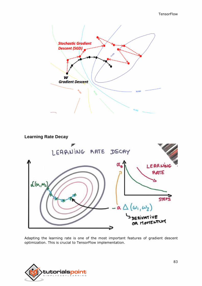
TensorFlow

83

Learning Rate Decay

Adapting the learning rate is one of the most important features of gradient descent

optimization. This is crucial to TensorFlow implementation.

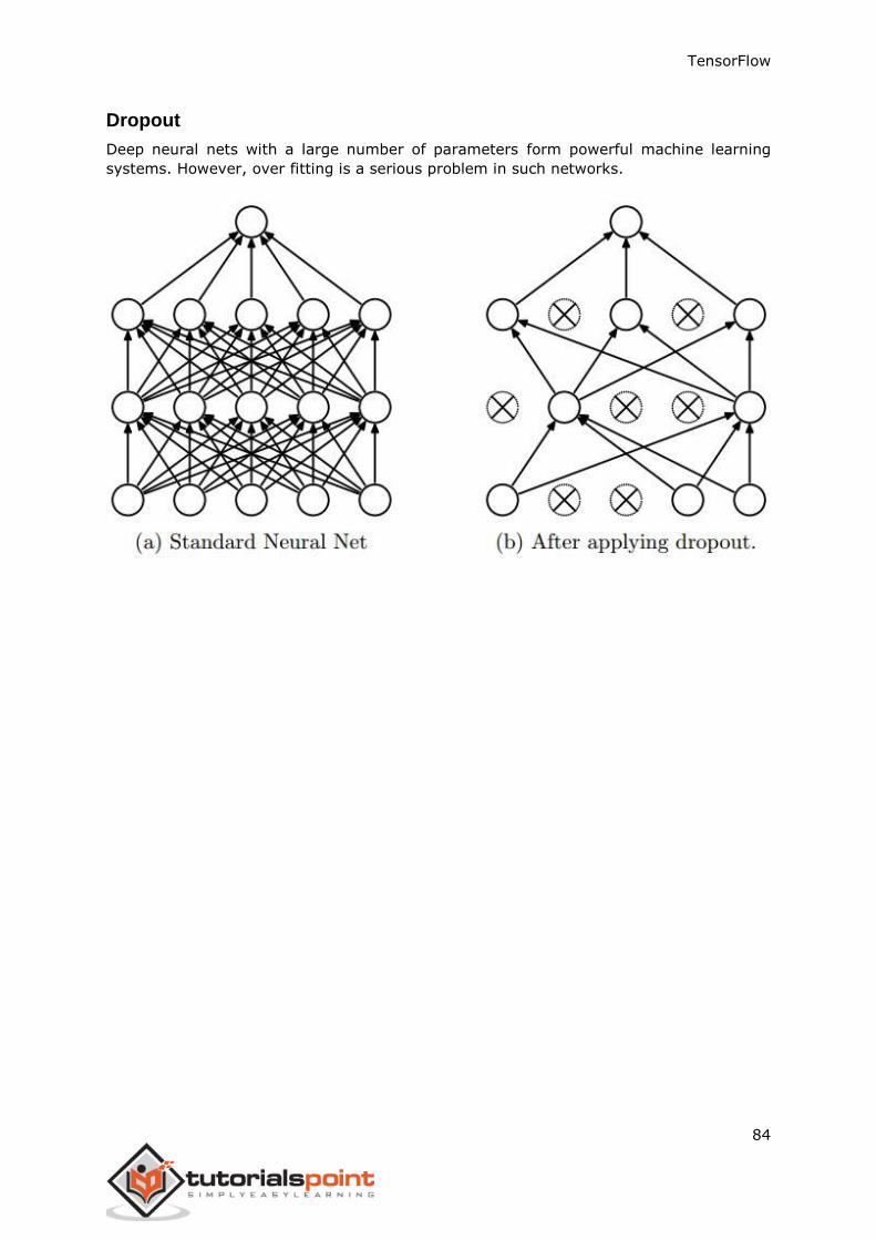
TensorFlow

84

Dropout

Deep neural nets with a large number of parameters form powerful machine learning

systems. However, over fitting is a serious problem in such networks.

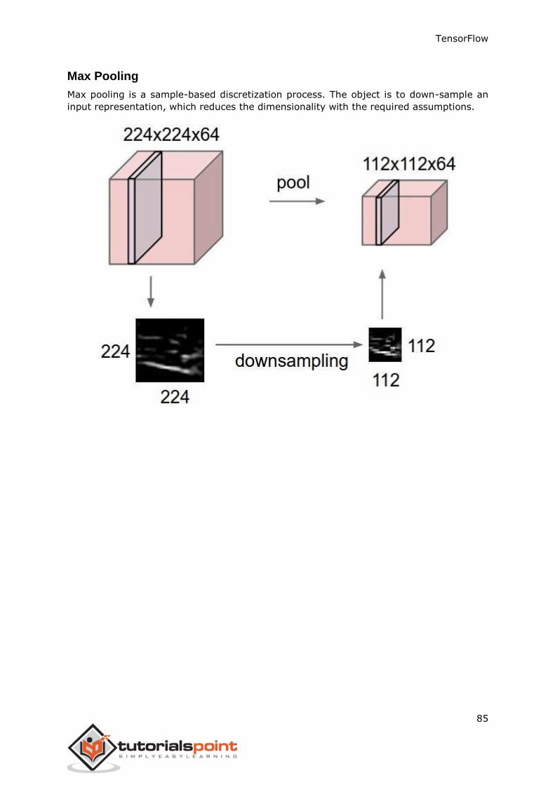
TensorFlow

85

Max Pooling

Max pooling is a sample-based discretization process. The object is to down-sample an

input representation, which reduces the dimensionality with the required assumptions.

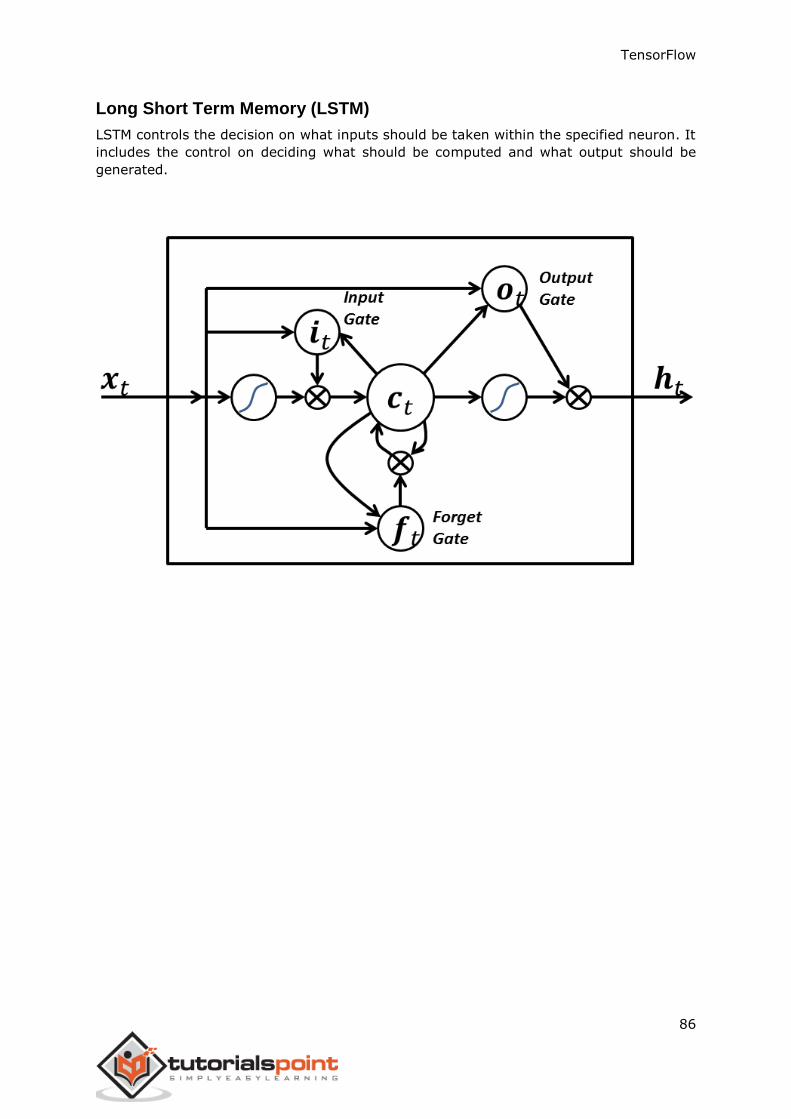
TensorFlow

86

Long Short Term Memory (LSTM)

LSTM controls the decision on what inputs should be taken within the specified neuron. It

includes the control on deciding what should be computed and what output should be

generated.