lthc.v22n2.86091 A poética de Losango cáqui, de Mário de ...


Tenório, Antônio Sandoildo Freitas. Phase transitions and thermodynamics of quasi-one-dimensional quantum rotor and spin systems / Antônio Sandoildo Freitas Tenório. - Recife : O Autor, 2009. xix, 134 folhas: il. fig. Tese (doutorado) - Universidade Federal de Pernambuco. CCEN. Física, 2009. Inclui bibliografia e apêndice. 1. Magnetismo. 2. Rotores quânticos. 3.Transições de fase (física estatística). I. Título. 538 CDD (22.ed.) FQ 2010-001


iii
DEDICATION
I Dedicate this dissertation to my wife Maria Barros de Araujo Tenorio, for her
unwavering support through thick and thin.
To my children Antonio Sandoildo Freitas Tenorio Filho, Ana Angelica Barros
Tenorio, and Maria Catarina Barros Tenorio, big-time fans of their old man.
To my grandchildren Laura Natalia Freitas Cavalcante Tenorio (Lalaka), Marcos
Antonio Tenorio Ferro (Caquinho) and, last but not least, toddling Maria Eduarda
Tenorio Guerra Camboim (Duduka). That they never plod their way through life
as a banking employee as did their granddaddy, so help me God.
An excerpt I came across in one of Nobel-Prize-winner Knut Hamsun’s novels,
in a serendipitous reading session, around 1971:
”Es ist nicht leicht sich auf die Menschen zu verstehen und zu erklaren, wer klug
und wer verruckt ist. Gott bewahre uns alle davor, dass wir durchschaut werden.”
Any free translation whatsoever is misleading.
Doctoral Dissertation - Departamento de Fısica - UFPE

IN MEMORIAM
Jose Duarte Tenorio (my father),
Antonia Freitas Tenorio (my mother),
Jose Samuel Freitas Tenorio (my brother), and
Feliciano Pessoa de Moura (my brother-in-law),
who left us to be with God.

v
ACKNOWLEDGMENTS
First and foremost I am thankful to JESUS, NOSSA SENHORA, SANTA
MADRE PAULINA, FREI DAMIAO, FREI GALVAO, and my PADRINHO CICERO,
for everything in this life, good and almost good.
I am deeply grateful to professor Maurıcio Domingues Coutinho Filho, my su-
pervisor, adviser, friend; a man endowed with great competence and vast knowledge
of Physics.
I am grateful from the bottom of my heart to professor Rene Rodrigues Mon-
tenegro Filho, a computer virtuoso besides being a knowledgeable physicist, for his
invaluable support, on a daily basis, always a reliable friend, without whom this
dissertation would not be.
I am grateful to Fernando Antonio Nobrega Santos for being helpful whenever
needed.
I am grateful to Joao Liberato de Freitas for his invaluable support.
I am grateful to my lab colleagues Karlla, Fernanda, and Eglanio, for their bits
of help, which added up to a lot.
I am grateful to all teachers and employees of Departamento de Fısica, who
somehow have taken part in this project.
I am grateful to my wife and my children, always a source of strength and
inspiration that have prodded me along.
To CAPES, CNPq, Finep, and Facepe for the indispensable financial support.
Doctoral Dissertation - Departamento de Fısica - UFPE

vi
Abstract
We start by presenting the ground state phase diagram of q = 1/2 quantum-
rotor chains with the AB2 topology and with competing interactions (frustration)
calculated through cluster variational mean-field approaches. We consider two inter-
action patterns, named F1 and F2 models, between the quantum-rotor momentum
and position operators, which follow exchange patterns of known one-dimensional
spin-1/2 systems with a ferrimagnetic state in their phase diagrams. The spin-1/2
F1 model is known as the diamond chain and is experimentally related to the azurite
compound, while the spin-1/2 F2 model was recently shown to present a frustration-
induced condensation of magnons. We provide a detailed comparison between the
quantum-rotor phase diagrams, in single- and multi-site mean-field approaches, and
known results for the spin-1/2 models, including exact diagonalization (ED) and
density matrix renormalization group (DMRG) data for these systems, as well as
phase diagrams of the associated classical models.
Finally, we turn to the thermodynamics of ferrimagnetic alternating spin-1/2
spin-5/2 chains whose study raises great interest both in the theoretical and the
experimental fields nowadays. Results concerning the magnetic susceptibility, mag-
netization and specific heat of two types of chains were obtained through the finite-
temperature Lanczos method (FTLM), which were then compared with experimen-
tal data as well as theoretical results from semiclassical approaches and spin-wave
theories. The ground state is also explored through ED calculations.
Keywords: quantum rotors, spins, magnetism, phase transitions.
Doctoral Dissertation - Departamento de Fısica - UFPE

vii
Resumo
Iniciamos com a apresentacao do diagrama de fases do estado fundamental de
rotores quanticos com q = 1/2 situados em cadeias com topologia AB2 e dotadas de
interacoes competitivas (frustracao). Os resultados sao obtidos mediante tecnicas
de campo medio variacional sobre conjuntos de sıtios (cluster variational mean-field
approaches). Consideramos dois modelos de interacao, denominados modelos F1 e
F2, entre os operadores de momento e de posicao do rotor quantico, os quais seguem
padroes de troca de sistemas de spins 1/2 conhecidos com um estado ferrimagnetico
em seus diagramas de fase. O modelo F1 de spin 1/2 e conhecido como cadeia tipo
losango (diamond chain) e esta experimentalmente relacionado a azurita, enquanto
que para o modelo F2 de spin-1/2, mostrou-se recentemente que este apresenta
condensacao de magnons induzida por frustracao. Tecemos comparacao detalhada
entre os diagramas de fase do rotor quantico, nas metodologias de campo medio em
um unico sıtio e em muitos sıtios, incluindo dados de diagonalizacao exata (sigla
em ingles: ED) e de grupos de renormalizacao da matriz de densidade (sigla em
ingles: DMRG), e resultados conhecidos para os modelos de spin 1/2 como tambem
diagramas de fases de modelos classicos associados.
Finalmente, tratamos da termodinamica de duas cadeias ferrimagneticas alter-
nadas com spins 1/2 e 5/2, cujo estudo atualmente tem despertado grande interesse
nos campos tanto teoricos como experimentais. Os resultados referentes a suscepti-
bilidade magnetica, magnetizacao e calor especıfico das cadeias sao obtidos atraves
do metodo de Lanczos para temperaturas finitas (sigla em ingles: FTLM), que sao
entao comparados com os dados experimentais como tambem com resultados teoricos
de metodologias semiclassicas e teorias de ondas de spins. O estado fundamental das
Doctoral Dissertation - Departamento de Fısica - UFPE

viii
cadeias tambem e estudado mediante diagonalizacao exata (sigla em ingles: ED).
Palavras-chave: rotores quanticos, spins, magnetismo, transicoes de fases.
Doctoral Dissertation - Departamento de Fısica - UFPE

Contents
ACKNOWLEDGMENTS . . . . . . . . . . . . . . . . . . . . . . . . . . . v
1 Introduction 2
2 Quantum rotors on the AB2 chain with competing interactions 4
2.1 Introduction . . . . . . . . . . . . . . . . . . . . . . . . . . . . . . . . 4
2.2 Outline of the theory and methods . . . . . . . . . . . . . . . . . . . 18
2.3 Quantum rotors on the AB2 chain: single-site variational mean-field
approach on the unit cell . . . . . . . . . . . . . . . . . . . . . . . . . 22
2.4 Quantum rotors on the AB2 chain: the double-cell variational mean-
field approach . . . . . . . . . . . . . . . . . . . . . . . . . . . . . . . 36
2.4.1 Frustration F1 . . . . . . . . . . . . . . . . . . . . . . . . . . . 40
2.4.2 Frustration F2 . . . . . . . . . . . . . . . . . . . . . . . . . . . 45
2.5 Summary and conclusions . . . . . . . . . . . . . . . . . . . . . . . . 58
3 Ground state and thermodynamics of alternating quantum spin
chains 61
3.1 Introduction . . . . . . . . . . . . . . . . . . . . . . . . . . . . . . . . 61
3.2 Theoretical models and methods . . . . . . . . . . . . . . . . . . . . . 68
ix

CONTENTS x
3.3 Static properties of an alternating isotropic chain of quantum spins
1/2 and classical spins . . . . . . . . . . . . . . . . . . . . . . . . . . 72
3.3.1 Free energy . . . . . . . . . . . . . . . . . . . . . . . . . . . . 73
3.3.2 Two-spin correlations . . . . . . . . . . . . . . . . . . . . . . . 74
3.3.3 Evaluation of the classical correlations . . . . . . . . . . . . . 75
3.3.4 Evaluation of correlations comprising quantum spins . . . . . 78
3.3.5 Magnetic susceptibility . . . . . . . . . . . . . . . . . . . . . . 79
3.4 Alternating spin-1/2 spin-5/2 ferrimagnetic chains - ground state and
thermodynamics . . . . . . . . . . . . . . . . . . . . . . . . . . . . . . 83
3.4.1 Ground states - ED results . . . . . . . . . . . . . . . . . . . . 83
3.4.2 Thermodynamic quantities . . . . . . . . . . . . . . . . . . . . 89
3.5 Summary and conclusions . . . . . . . . . . . . . . . . . . . . . . . . 106
A Appendix 108
A.1 The Basis of monopole harmonics states . . . . . . . . . . . . . . . . 108
A.2 Finite-temperature Lanczos method (FTLM) . . . . . . . . . . . . . . 113
A.2.1 Overview . . . . . . . . . . . . . . . . . . . . . . . . . . . . . 113
A.2.2 Adjusting FTLM . . . . . . . . . . . . . . . . . . . . . . . . . 118
Bibliography 120
Doctoral Dissertation - Departamento de Fısica - UFPE

List of Figures
2.1 MF phase diagram of H ′rot as a function of the couplings J and K
at MZ = 4, g = 1, and α = 1; Z is the coordination number of
the lattice. Thin lines represent second-order transitions while thick
lines are first order. The quantized ferromagnetic phases QFl have
magnetic moment per site l; there is an infinite sequence of such
phases for all integer l > 0 at larger values of K, and only the first two
are shown. The phases have the following ground-state expectation
values, up to a global O(3) rotation: gapped quantum paramagnet
(GP): < Lµ >= 0, < nµ >= 0; quantized ferromagnet (QFl): <
Lz >= l, < nz > 6= 0; < Lx,y >= 0, < nx,y >= 0; Neel (N): < Lµ >=
0, < nz > 6= 0, < nx,y >= 0; canted (C): < Lx,z > 6= 0, < nx,z > 6= 0,
< Ly >= 0, < ny >= 0 (reproduced from Ref. [47]). . . . . . . . . . . 14
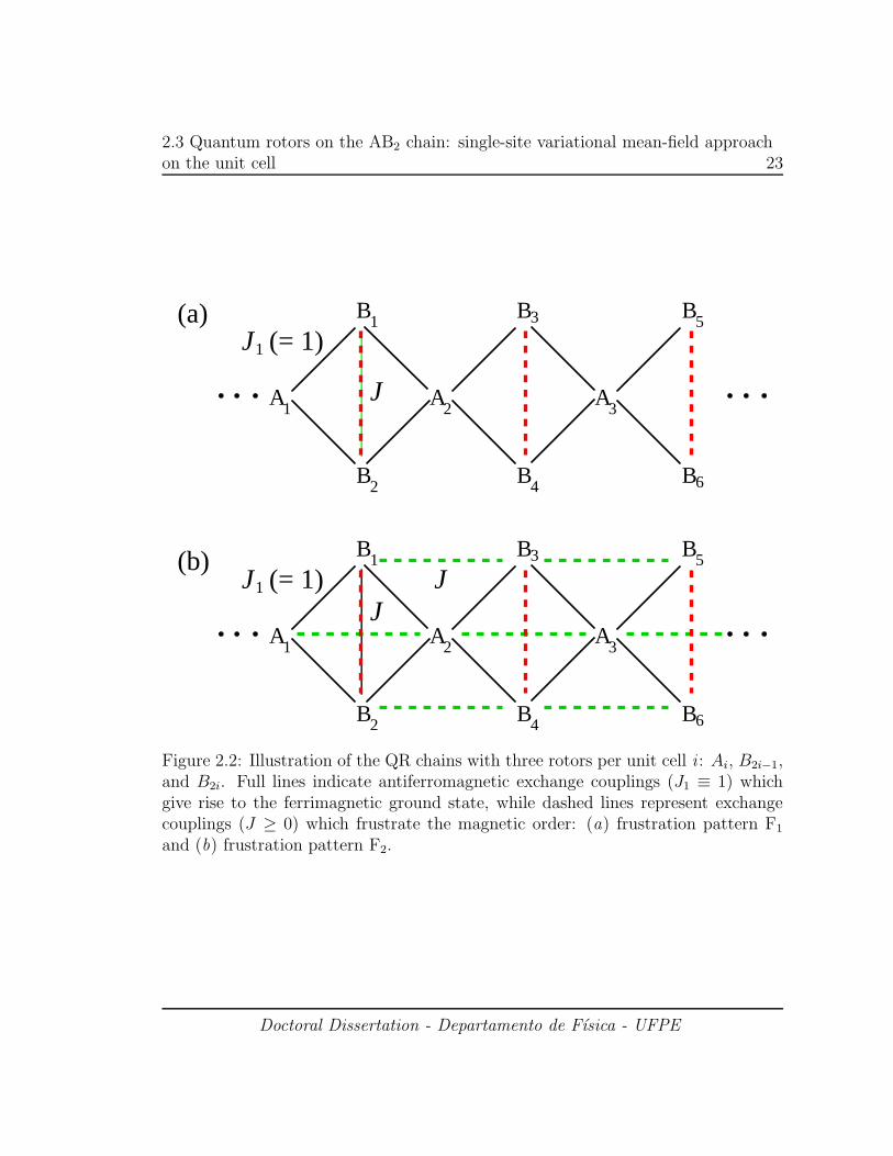
2.2 Illustration of the QR chains with three rotors per unit cell i : Ai,
B2i−1, and B2i. Full lines indicate antiferromagnetic exchange cou-
plings (J1 ≡ 1) which give rise to the ferrimagnetic ground state, while
dashed lines represent exchange couplings (J ≥ 0) which frustrate the
magnetic order: (a) frustration pattern F1 and (b) frustration pattern
F2. . . . . . . . . . . . . . . . . . . . . . . . . . . . . . . . . . . . . . 23
xi

LIST OF FIGURES xii
2.3 Frustration F1. Two-point MF momentum products [(a) M ≡ 0,
(c) M ≡ 1] between the indicated rotors and MF energy curve [(b)
M ≡ 0, (d) M ≡ 1], where we have drawn straight (full) lines to
show that at J = 1 the system steers away from the linear regime
that prevails for J ≤ 1 and so a phase transition takes place. Full and
dashed lines in (a) and (c) indicate the results of the classical vector
model. Dashed lines in (b) and (d) are guides to the eye. . . . . . . . 28
2.4 Frustration F2. Same as in Fig. 2.3. . . . . . . . . . . . . . . . . . . . 29
2.5 Two-point MF momentum products for frustration F1. Here an in-
appropriate choice of the parameters g = α = 1 and a Hilbert space
truncated at ℓ = 1/2 was made. One cannot make any physical pat-
tern out of the plots. . . . . . . . . . . . . . . . . . . . . . . . . . . . 30
2.6 Two-point MF momentum products for frustration F1. Here we show
a choice of the parameters g = α = 1 with a Hilbert space truncated
at ℓ = 6.5. The momenta are scaled up to the highest ℓ. . . . . . . . . 31
2.7 Classical vector configuration. The angle θ is the unique order pa-
rameter. . . . . . . . . . . . . . . . . . . . . . . . . . . . . . . . . . . 34
2.8 Two-point MF momentum products for frustration F1. Here we show
a choice of the parameters g = α = 1 with a Hilbert space truncated
at ℓ = 5.5. M = 10 in the frustration coupling and M = 1 elsewhere.
The system behaves just like the one depicted in Fig. 2.3, but the
transition takes place at Jt ≈ 1.8, i.e., with a shift to the right hinted
at by Eq. (2.38). . . . . . . . . . . . . . . . . . . . . . . . . . . . . . 35
Doctoral Dissertation - Departamento de Fısica - UFPE

LIST OF FIGURES xiii
2.9 Illustration of the ground states found for the spin-1/2 diamond chain[57]
as J is increased from 0. (a) The ferrimagnetic (FERRI) state. (b)
The tetramer-dimer (TD) state, where rectangles represent singlet
tetramers and ellipses singlet dimers. (c) The dimer-monomer (DM)
state. There are two first-order phase transitions: at J = 0.909
(FERRI/TD) and J = 2 (TD/DM). . . . . . . . . . . . . . . . . . . . 41
2.10 Spin-1/2 diamond chain: ED results for the correlation functions be-
tween spins at a central cluster of a system with 28 sites. Dashed
lines are guides to the eye. . . . . . . . . . . . . . . . . . . . . . . . . 42
2.11 Spin-1/2 diamond chain: ED results for the (a) average ground-state
energy and (b) rescaled total spin of a system with 28 sites. Phase
transitions occur at J = 0.88 and J = 2.0, both of first order. Dashed
lines are guides to the eye. . . . . . . . . . . . . . . . . . . . . . . . . 43
2.12 QR momentum correlations calculated by using the double-cell vari-
ational MF approach for frustration F1. One notices the phase se-
quence FERRI↔TD↔DM, with first-order transitions at J = 0.68
and J = 2. Dashed lines are guides to the eye. . . . . . . . . . . . . . 46
2.13 Quantum rotors by using the double-cell variational MF results for
frustration F1: (a) the energy plot (E0 = 1962) shows cusps at the
first-order transition points J = 0.68 and J = 2.0; (b) expectation
value of the total angular momentum per unit cell. Dashed lines are
guides to the eye. . . . . . . . . . . . . . . . . . . . . . . . . . . . . . 47
Doctoral Dissertation - Departamento de Fısica - UFPE

LIST OF FIGURES xiv
2.14 Quantum rotors with frustration F1: average singlet density per unit
cell for the momenta of the B sites at the same unit cell. One can
make out the three phases: FERRI, TD, and DM, as well as pertinent
transitions. Dashed lines are guides to the eye. . . . . . . . . . . . . . 48
2.15 QR momentum correlations calculated by using the double-cell vari-
ational MF approach for frustration F2. One can distinguish three
major phases: FERRI, CANTED, and the decoupled AF chain lad-
der system, with transitions occurring around J = 0.35 and J = 0.75.
Dashed lines are guides to the eye. . . . . . . . . . . . . . . . . . . . 49
2.16 Quantum rotors by using the double-cell variational MF results for
frustration F2: (a) energy and (b) expectation value of the total an-
gular momentum per unit cell. The inset shows details of the phase
transition around J = 0.35. Dashed lines are guides to the eye. . . . . 50
2.17 Illustration of the major QR ground states for frustration F2: (a)
FERRI; (b) CANTED; (c) AF, which is composed of two decoupled
1D systems: a linear chain (A sites) and the two-legged ladder (B sites). 52
2.18 Quantum rotors with frustration F2: average singlet density per unit
cell for the momentum correlations at B sites along the same rung
of the ladder. The inset shows details of the phase transition around
J = 0.36. . . . . . . . . . . . . . . . . . . . . . . . . . . . . . . . . . . 54
Doctoral Dissertation - Departamento de Fısica - UFPE

LIST OF FIGURES xv
2.19 (a) Pitch angle for the quantum spin-1/2 model calculated through
ED, DMRG, and for the minimum energy configuration of the clas-
sical vector model with two order parameters: q (pitch angle) and
θ (canting angle). The transition points estimated in Ref. [59] are
indicated. (b) Momentum dot products (i = 1, 2, and l denotes the
unit cell) in the minimum energy configuration of the classical vector
model. . . . . . . . . . . . . . . . . . . . . . . . . . . . . . . . . . . . 57
3.1 Temperature dependence of χmT for the first bimetallic chain (CuM-
nDTO) [93, 94], where χm is the molar susceptibility and T is the
temperature. Squares represent experimental points, and the full line
is a plot of Eq. (3.35). A minimum occurs at T = 130K. Reproduced
from Seiden[141]. . . . . . . . . . . . . . . . . . . . . . . . . . . . . . 66
3.2 Schematic representation of the Hamiltonian and ground-state mag-
netic order of the (a) sS and (b) ssS alternating chains. In Seiden’s
paper [141] the larger spin (longer arrow) is a classical quantity, the
other one being quantum. . . . . . . . . . . . . . . . . . . . . . . . . 82
3.3 One-magnon bands of the sS chain. Full lines are spin-wave results
from Ref. [143], while dashed lines are guides to the eyes. Sz = SG−1
for the lower band, while Sz = SG + 1 for the upper one. Inset: Size
dependence of the antiferromagnetic gap ∆, which is estimated to be
∆ = 4.9046J in the thermodynamic limit. . . . . . . . . . . . . . . . 85
Doctoral Dissertation - Departamento de Fısica - UFPE

LIST OF FIGURES xvi
3.4 One-magnon bands of the ssS chain with J′
= 1.7J . Dashed lines are
guides to the eyes.Sz = SG − 1 for the lower band, while Sz = SG + 1
for the upper one. Inset: Size dependence of the antiferromagnetic
gap ∆, which is estimated to be ∆ = 3.88J in the thermodynamic
limit. . . . . . . . . . . . . . . . . . . . . . . . . . . . . . . . . . . . . 86
3.5 Magnetization per cell M normalized by its saturation value Msat =
3gµB as a function of applied magnetic field B in units of J/gµB at
T = 0 for the sS chain. We have set J = 44.8K (see Subsection 3.4.2,
Fig. 3.10). The first plateau ends at bc = gµBBc/J ≈ 4.9 which
implies that Bc ∼ 150 T. On the other hand, the saturation field
BS = JbS/gµB ∼ 200 T. . . . . . . . . . . . . . . . . . . . . . . . . . 87
3.6 Magnetization per cell M normalized by its saturation value Msat =
3.5gµB as a function of applied magnetic field B in units of J/gµB
at T = 0 for the ssS chain with J′
= 1.7J (see Subsection 3.4.2,
Fig. 3.11). The first plateau ends at bc = gµBBc/J ≈ 3.9 which
implies that Bc ∼ 400T . On the other hand, the saturation field
BS = JbS/gµB ∼ 600T . . . . . . . . . . . . . . . . . . . . . . . . . . . 88
Doctoral Dissertation - Departamento de Fısica - UFPE

LIST OF FIGURES xvii
3.7 Magnetization per mol for the sS chain as a function of the applied
magnetic field B for T = 4.2 K. Experimental data of the compound
CuMnDTO from Ref. [94, 141]. FTLM for a system with N = 16,
J = 44.8 K and g = 1.93. Quantum paramagnet: fitting of the
FTLM data to the magnetization per mol of a quantum paramagnet
(Brillouin function) with total spin S. Taking g = 1.93, the best fit
implying S = 15.8. The inset serves the purpose of showing how the
finite temperature modifies the field-induced Lieb-Mattis ferrimag-
netic ground state. . . . . . . . . . . . . . . . . . . . . . . . . . . . . 89
3.8 FTLM results for the magnetization normalized by its value at T =
0(M(T = 0) = 1.5 per cell) for the ssS chain as a function of the
normalized applied magnetic field at T = 0.1J . The system size is
N = 18. Quantum paramagnet: fitting of the FTLM data to the
expected curve for a quantum paramagnet (Brillouin function) with
total spin S, the best fit implying S = 8.74. The inset serves the
purpose of showing how the finite temperature modifies the field-
induced Lieb-Mattis ground state. . . . . . . . . . . . . . . . . . . . . 90
3.9 Product of the susceptibility per site χ and the temperature T for the
sS chain with N = 16. In the inset we present the derivative of this
curve in the temperature range in which its minimum, Tmin = 2.9J ,
is found. . . . . . . . . . . . . . . . . . . . . . . . . . . . . . . . . . 92
Doctoral Dissertation - Departamento de Fısica - UFPE

LIST OF FIGURES xviii
3.10 Product of the molar susceptibility χm and temperature T as a func-
tion of T for the sS chain. Experimental data for the compound
CuMnDTO from Ref. [141]. Semiclassical susceptibility according to
Eq. (3.35): J = 59.7 K, S = 2.5 and g = 1.9. FTLM results for a
system with N = 16, the best fit to the experimental data implies
J= 44.8 K and g = 1.90. . . . . . . . . . . . . . . . . . . . . . . . . . 93
3.11 Product of the susceptibility per site χ and the temperature T for
the ssS chain with N = 18. (a) The numerical data, for the indicated
values of J′
/J , are compared with the experimental data for the com-
pound MnNN from Ref. [111] by arbitrarily defining J = 100K, in
order to enhance graph readability. (b) χT for J′
= 1.7J and its
derivative, shown in the inset. The minimum of this curve is found
at Tmin = 1.7J . . . . . . . . . . . . . . . . . . . . . . . . . . . . . . . 94
3.12 Product of the molar susceptibility χm and temperature T as a func-
tion of T for the ssS chain. Experimental data of the MnNN com-
pound from Ref. [111]. Semiclassical susceptibility according to Eq.
(3.38): J = 144 K, J′
= 248 K, S = 2.5 and g = 2.0. FTLM results
for a system with N = 18, the best fit to the experimental data im-
plies J = 150 K and J′
= 255 K, while g(= 2.0) is not taken as a
fitting parameter. . . . . . . . . . . . . . . . . . . . . . . . . . . . . . 95
3.13 Specific heat per site as a function of temperature T for sS and the
ssS, with J′
= 1.7J , chains. The full lines are the respective Schottky
specific heats (Eq. (3.41)). Dashed lines are guides to the eye. . . . . 97
Doctoral Dissertation - Departamento de Fısica - UFPE

LIST OF FIGURES xix
3.14 Specific heat per site as a function of temperature T of the sS chain,
for various intensities of the applied magnetic field, as indicated. The
height position wanders to the right and then back to the left. . . . . 98
3.15 (a) Specific heat per site as a function of temperature T of the sS
chains, for various intensities of the applied magnetic field. The full
lines represent the respective Schottky specific heat. (b) Schottky δB
(Eq. (3.41)) and chain ∆B gaps as functions of the applied field (Eq.
(3.43)). At B/(J/gµB) ≈ 3.5, we find that δB ≈ ∆B. . . . . . . . . . 99
3.16 Product of the susceptibility per site χ and the temperature T squared
for the ferromagnetically coupled linear chain in the low temperature
region, T < J . Spin-wave result up to second order in T/J from
Ref. [147]. The temperature range T < 0.1J for which the spin-wave
result is almost exact is shown in the inset. The FTLM calculations
were made on spin-1/2 ferromagnetic linear chains. . . . . . . . . . . 102
3.17 Product of the normalized susceptibility χ per unit cell and the tem-
perature T squared. FTLM data were obtained for the indicated
system sizes. The semiclassical result comes from Eq. (3.35). Mod-
ified spin-wave results up to second order in T/J from Ref. [149].
The FTLM result for 0.5 < TJ< 0.9 is fitted to a function of the
form [53+a0(
TJ)
1
2 +a1(TJ)] and a0 and a1 are estimated to be 1.28 and
0.69, respectively. Experimental results were normalized by taking
J = 59.7 K (g = 1.9) and J = 44.8 K (g = 1.85), which must be
compared with the semiclassical and FTLM results, respectively. . . . 104
Doctoral Dissertation - Departamento de Fısica - UFPE

LIST OF FIGURES 1
3.18 Product of the susceptibility per site χ and the temperature T squared
for the sS chain. Inset: Temperature region 0 < (T/J) < 2. Best
fit, in the region T > 0.8J , to a function as a0 + a1x0.5 + a2x +
a3x1.5 + a4x
2 + a5x2.5, with x = T/J , implies a0 = 1.73, a1 = 0.12,
a2 = −1.83, a3 = 2.40, a4 = −0.65 and a5 = 0.06; while if the fitting
function is a0 + a1x+ a2x2 + a3x
3 + a4x4 + a5x
5, the best parameters
are a0 = 1.4211, a1 = 0.0289, a2 = 0.4255, a3 = −0.0623, a4 = 0.0046
and a5 = −0.0001. . . . . . . . . . . . . . . . . . . . . . . . . . . . . 105
A.1 The behavior of the product of the susceptibility per site χ and the
temperature T of the ssS chain with N = 18 and J = 1.5J′
. The
number of states M taken in each random sampling is 50 and the
total number of random samples R is indicated in the figure. Each
curve is the result of one running of the FTLM algorithm with the
indicated parameters, thus there are 10, 5, 2 and 1 runnings in figures
(a), (b), (c) and (d), respectively. The precise value of χT for this
system size as T → 0, limT→0 χT = 5/3, is indicated by the symbol
3. The inset of (a) and (b) show the region near the minimum of the
curve, while the inset of (c) and (d) show the region near T = 0. . . . 119
Doctoral Dissertation - Departamento de Fısica - UFPE

Chapter 1
Introduction
This dissertation is composed of two main chapters where we treat correlated
subjects.
In Chapter 2, we present the idea of quantum rotors and their importance in cur-
rent research. We then study the ground state phase diagram of q = 1/2 quantum-
rotor chains with the AB2 topology and with competing interactions (frustration)
calculated through cluster variational mean-field approaches. A detailed compari-
son is provided which emphasizes the similarities between the quantum-rotor phase
diagrams, in single- and multi-site mean-field approaches, and known results for the
spin-1/2 models, including exact diagonalization and density matrix renormalization
group data for these systems, as well as phase diagrams of the associated classical
models. The main results of this chapter were condensed in the article published by
Physical Review B [155].
In Chapter 3, we finally turn to the thermodynamics of ferrimagnetic alternat-
ing spin-1/2 spin-5/2 chains whose study raises great interest both in the theoretical
2

3
and the experimental fields nowadays. We start out with a brief review showing the
relevance of the pertinent materials in decades of intensive research in the area of
molecular magnetism. Then results concerning the magnetic susceptibility, magne-
tization and specific heat of two types of chains are obtained through the finite-
temperature Lanczos method (FTLM). These are compared with experimental data
as well as theoretical results from semiclassical approaches and spin-wave theories.
Work is still being done until we have produced material enough that may warrant
the submission of a new article on the subject.
In the end of each chapter we present the respective summary and conclusions.
Doctoral Dissertation - Departamento de Fısica - UFPE

Chapter 2
Quantum rotors on the AB2 chain
with competing interactions
2.1 Introduction
Rotors are tridimensional rigid objects such as a top or a gyroscope (which may have
freedom in all three axes) used to explain rotating systems as well as for maintain-
ing and measuring orientation, based on the principles of angular momentum. To
determine their orientation in space three angles are required (the Euler angles, for
instance). Special among these is the linear rotor, which consists of two point masses
located at fixed distances from the center of mass. The object is three-dimensional,
but requires only two angles to describe its orientation. The quantum version of this
model is a useful point of departure for the study of the rotational transitions of
diatomic molecules (zeroth-order model). A more accurate description of the energy
of the molecule would accordingly include possible variations in bond length due to
rotations or anharmonicity in the potential due to vibrations. As will be seen shortly
4

2.1 Introduction 5
below, this model and its ad hoc variations exhibit interesting physics and lends itself
admirably to the understanding of sundry other physical systems, far outreaching
its basic use for the study of the rotational energy of diatomic molecules.
We now provide a first glimpse of the quantum mechanics of the quantum linear
(rigid) rotor (QLR). This is indeed the case of the spherical rotor, where the three
components of the moment-of-inertia tensor are equal (a symmetric rotor or top has
two equal components and the asymmetric one boasts three different components.
The symmetric top can be analytically addressed by using Wigner D-matrices; the
asymmetric case does not have an exact solution. The rotational energy depends on
the moment of inertia, I, in the center-of-mass reference frame,
I = µR2 (2.1)
where µ is the reduced mass of the molecule and R is the distance between the two
atoms. In addition to its usefulness, the QLR is a very simple model and one case
where the Schrodinger equation can be solved analytically. In a field-free space, the
Hamiltonian operator is given in terms of spherical coordinates and reads
H =~
2
2IL
2= −~
2
2I
[
1
sin θ
∂
∂θ(sin θ
∂
∂θ) +
1
sin2 θ
∂2
∂φ2
]
, (2.2)
where ~ is Planck’s constant divided by 2π, and θ and φ are the polar and azimuthal
angles, respectively. The eigenvalue equation becomes
HY ml (θ, φ) =
~2
2Il(l + 1)Y m
l (θ, φ), (2.3)
where the notation Y ml (θ, φ) stands for the set of the spherical harmonics. The
Doctoral Dissertation - Departamento de Fısica - UFPE

2.1 Introduction 6
energy spectrum is given by the eigenvalues
El =~
2
2Il(l + 1), (2.4)
and is independent of m (magnetic quantum number). The energy is indeed (2l+1)-
fold degenerate, because functions with fixed l (azimuthal quantum number) and
m = −l,−l+1, . . . , l have the same energy. Quantum rotors may be seen as existing
almost freely or coupled by intrinsic potentials (dipole interactions, etc) or acted
upon by potentials inherent in the host medium. In many cases, the quantum
planar rotor (QPR), i.e., endowed with only one degree of freedom, is used.
The very simple idea of the quantum rotor presented so far can be viewed as a
fundamental model closest to the natural entity it may be bound to represent: the
molecule. Systematic studies on the rotation of molecules supported by the quantum
theory date back to Dennison [1], and Kronig and Rabi [2], who provided matrix
and wave-mechanics analytical solutions to the rigid rotator (symmetrical top), both
within a year or so of the respective fledgling quantum theory formulations. Later, an
important study by Pauling [3] discussed the wave equation for a diatomic molecule
in a crystal and tried to provide experimental interpretation of the results.
The microscopic dynamics of quantum rotors has been ever since extensively
studied in view of its enormous physical and chemical interest and has always been
a source of new physics. Real physical systems like molecular cryocrystals, ad-
sorbed monolayers of diatomic molecules such as H2, HD, D2, N2, CO, and F2 can
be described by the QLR model [4–6]. The QLR manifests also nontrivial quan-
tum properties such as quantum orientational ordering [6, 7], quantum orientational
melting [4, 6, 8, 9], reentrant behavior [10], and discontinuity points on the phase
diagram [11]. In the latter it is reported evidence for the novel phase behavior in
Doctoral Dissertation - Departamento de Fısica - UFPE
2.1 Introduction 7
quantum rotors: at zero temperature, instead of an end critical point of the liquid-
gas type, the phase transition line in a certain range of crystal fields displays two
critical points with a discontinuity (”hole”) between them. By endowing the QLR
with an intrinsic angular momentum (spin) it is possible to study the unusual ther-
modynamics and magnetic properties of molecular crystals containing magnetically
active molecules or molecular groups [12].
The notion of quantum rotors can also be advantageously applied to the un-
derstanding of interstitial oxygen impurities in crystalline germanium, where oxy-
gen atoms are quantum-mechanically delocalized around the bond center position
[13, 14]. Also the correlated dynamics of coupled quantum rotors (Ge2O units)
carrying electric dipole moments is used to gain insight into the peculiar and non-
trivial low-temperature properties of doped germanium [15]. The rotation of oxy-
gen impurities around the Ge-Ge axis has been experimentally observed by phonon
spectroscopy [16]. While the rotation of oxygen impurities in Ge is weakly hindered
by an azimuthal potential caused by the host lattice, several materials are known
to show a free rotation of molecules. An example is ammonia groups in certain
Hofmann clathrates M(NH3)2M’(CN)4-G [17–19], usually abbreviated as M-M’-G,
where M and M’ are divalent metal ions and G is a guest molecule. Nearly free
uniaxial quantum rotation of NH3 has been observed for the first time in Ni-Ni-
(C6D6)2 by inelastic neutron scattering [17]. It is also known that the phase II
[20] of solid methane as well as methane hydrates [21] show almost free rotation of
CH4 molecules. A surprising variation of the linewidth has been observed for Ni-Ni-
(C12H10)2 [22], which can be interpreted as a novel line-broadening mechanism based
on rotor-rotor couplings [23]. The linewidths of methane in hydrates show inhomo-
geneous broadening owing to the dipolar coupling with water molecules [24]. The
Doctoral Dissertation - Departamento de Fısica - UFPE

2.1 Introduction 8
theory of the damped rotation of methyllike atomic groupings and more complex
molecules such as benzene rings is developed through the use of hindered (N-fold)
quantum rotors in contact with a thermal bath [25, 26].
Arrays of surface-mounted quantum rotors with electric dipole moments are of
particular interest because dipole-dipole interactions can be controlled and even de-
signed to yield a specific behavior such as ferroelectricity. Ordered two-dimensional
arrays of dipole rotors yield either ferroelectric or antiferroelectric ground states,
depending on the lattice type, while disordered arrays are predicted to form a glass
phase [27, 28]. These facts prop up the role of quantum rotors as a fundamental
element of molecular machines, an old and new field of endeavor of both synthetic
chemistry and nanotechnology [29–33].
The kicked rotor has played a central role in the research of both classical and
quantum chaos (which is defined as the quantum behavior of a system whose clas-
sical counterpart is chaotic). A kicked rotor is formed by a particle revolving in a
fixed circular orbit and subject to an instantaneous force (a kick) that is applied pe-
riodically. The driven rotor is operated on by pulses of any form (generally strong).
Despite its apparent simplicity, the quantum kicked rotor has very remarkable dy-
namical properties [34–38]. Since its experimental realization in 1995 [39], a great
number of studies have been produced involving dynamical localization, quantum
transport, ratchets, chaos-assisted tunneling, and classical and quantum resonances.
Quantum resonances in turn have been used in understanding fundamental aspects
of quantum chaos such as quantum stabilization or measurements of gravitation
[37]. High-order quantum resonances have also been observed recently both with
laser-cooled atoms and a Bose-Einstein condensate [40–42].
We now move up a notch toward a more elaborated rotor model that finds
Doctoral Dissertation - Departamento de Fısica - UFPE

2.1 Introduction 9
applications specially in the study of quantum phase transitions, the main goal
of this work as far as quantum rotors and spin systems are concerned. So, we
present another glimpse of the quantum mechanics involved [43]. Each rotor can be
constructed as a particle constrained to move on the surface of an N -dimensional
sphere. Here we treat our Euclidean space as having (N > 1) dimensions, a quite
natural extension nowadays. We thus have the so-called O(N) quantum rotor model.
The orientation of each rotor is represented by an N -component unit vector ni
satisfying:
n2 = 1. (2.5)
The caret notation should be reminiscent of the fact that the rotor orientantion is
a quantum operator, while i indexes the site whereupon the rotor resides. For the
time being, it will be considered an infinite number of such rotors placed on the
sites of a d-dimensional lattice. Each rotor possesses a linear momentum pi and
constraint (2.5) obliges it to be tangent to the surface of the N -dimensional sphere
n · p = 0. (2.6)
The rotor position and momentum obey the canonical commutation relations:
[nα, pβ] = i~δαβ . (2.7)
It seems more convenient to work with the N(N − 1) components of the angular
momentum tensor:
Lαβ = nαpβ − nβ pα. (2.8)
Their commutation relations follow directly from Eqs. (2.7) and (2.8). Of foremost
Doctoral Dissertation - Departamento de Fısica - UFPE

2.1 Introduction 10
importance is the N = 3 case. The angular momentum can be more conveniently
expressed as
Lα = (1/2)ǫαβγLβγ, (2.9)
or alternatively
Lα = −i~ǫαβγnβ∂
∂nγ, (2.10)
where ǫαβγ stands for the Levi-Civita tensor (totally antisymmetric tensor, with
ǫ123 = 1). Obviously the constraint Eq. (2.6) carries through to
n · L = 0. (2.11)
Accordingly, the commutation relations between operators standing on the same site
follow:
[Lα, Lβ] = i~ǫαβγLγ ,
[Lα, nβ] = i~ǫαβγnγ , (2.12)
[nα, nβ] = 0;
operators situated on different sites commute. The rotor dynamics is governed by
its kinetic energy term, which may be expressed as
HK =1
2IL2 → g
2L2, (2.13)
where I is the moment of inertia and we have introduced a coupling g. The Hamil-
tonian HK can be diagonalized for general values of N by making use of group
theory. For N = 3, the eigenvalues were already shown through Eq. (2.3) and Eq.
Doctoral Dissertation - Departamento de Fısica - UFPE

2.1 Introduction 11
(2.4). Interesting effects show up when a potential energy term coupling the rotors
together is added. Then we construct the Hamiltonian, which has been object of
intensive study:
Hrot =g
2
∑
i
L2i + Jij
∑
<ij>
ni.nj , (2.14)
where the notation < ij > indicates the sum over nearest neighbors, and Jij repre-
sent couplings between the respective rotor orientations. A generalization thereof,
with the addition of novel couplings, will be considered shortly.
Quantum transitions of models based on Eq. (2.14) and its Ising-model coun-
terpart have been extensively studied for decades. A review of the theoretical in-
vestigations as well as their experimental connotations can be found in the book by
Sachdev [43]. The effort to understand the model goes on and every now and then
rich and interesting phase diagrams unfold, which yield invaluable insights into the
real physical systems. So, quantum rotors have been studied and their phase dia-
gram investigated through renormalization group techniques [44], the dynamics and
thermodynamics of interacting one-dimensional quantum rotors with emphasis on
equilibrium and non-equilibrium properties have been explored through a mean-field
(MF) model [45], the quantum phase transitions of a site-diluted two-dimensional
O(3) rotor model have been worked out through Monte Carlo simulations [46], just
to mention a few additional important studies.
Dating back to a work by Sachdev and Senthil [47] there exists a generalization
of the Hamiltonian in Eq. (2.14). In its most general terms, it is given by
H ′rot =
g
2
∑
i
[L2i +α(L2
i )2]+
∑
<ij>
[Jijni · nj +KijLi · Lj +Mij(ni · Lj + nj · Li)], (2.15)
where for O(3) rotors the three-component unit position vector (operator) and
Doctoral Dissertation - Departamento de Fısica - UFPE

2.1 Introduction 12
the canonically conjugate angular momentum (operator) are explicitly given by
n = (nx, ny, nz), L = (Lx, Ly, Lz), respectively, and the couplings g, α, J , K e M are
all positive. The introduction of the couplings K and M in Eq.(2.15) enriches the
model and yields novel results in relation to systems modeled by the Hamiltonian of
Eq. (2.14). A fundamental property of H ′rot is that the three charges (µ = x, y, z)
Qµ =∑
i
Liµ, (2.16)
commute with it, and are therefore conserved. A quartic term, with coefficient gα, is
inserted and acts as an inhibitor of contributions of unimportant high-energy states.
For in-depth considerations of the model, a knowledge of the pertinent discrete
symmetries may afford one a vantage point. In this respect, the model boasts time-
reversal symmetry, and for the special case M = 0, spatial inversion (parity) is also
present. Time-reversal symmetry is realized by the transformations:
τ : Lµ → −Lµ, nµ → nµ, (2.17)
and parity by
π : Lµ → Lµ, nµ → −nµ. (2.18)
The MF phase diagram of H ′rot was then reproduced in Fig. 2.1, where all the
phases are duly described. The figure shows, for instance, that the distinction
between the GP and the N phases can only be made through the value of < nz >,
which happens to be zero in the former and nonzero in the latter phase. This phase
diagram exemplifies the case of rotors with q = 0, that is, rotors whose minimum
angular momentum is zero. We see that there is a gap to all excitations. The phase
Doctoral Dissertation - Departamento de Fısica - UFPE

2.1 Introduction 13
diagram for q = 1/2 rotors, that is, rotors whose minimum angular momenta has the
value l = 1/2 bears a close resemblance with the one presented here, except for one
important difference: it does not possess an energy gap (the GP phase is absent), as
is reasonable to expect so. The momentum-state tower of each rotor is not limited
(only the first two QFl phases are shown), and this fact leads to the interpretation
of a rotor as an effective quantum degree of freedom for the low energy states of
a small number (even, when 2q is pair, and odd, if 2q is odd) of closely coupled
electrons. In this work we shall relinquish this interpretation and adopt a simpler
one: we will attempt to ”lure” each rotor into representing just a single spin posed
on each site. The more precise meaning of q shall be addressed in a short while.
The connection between O(N) quantum-rotor (QR) and spin models on
d-dimensional lattices has proved very useful in the context of phase transitions
[43, 48]. About three decades ago, Hamer, Kogut and Susskind [49] mapped two-
dimensional O(N) Heisenberg models (N = 2, 3 and 4) onto the corresponding [(1+1)
spatial and time dimensions] nonlinear-sigma or QR models. The critical behavior
was then inferred using strong-coupling expansion (high-temperature, g = kT/J → ∞,
where J is the spin coupling): a Kosterlitz-Thouless transition for the O(2) model
and a prediction of critical points at zero coupling (Pade continued) for both O(3)
and O(4) models. On the other hand, by mapping O(3) antiferromagnetic (AF)
Heisenberg chains onto nonlinear sigma models in the semiclassical weak-coupling
limit (g = 2/S, S → ∞), Haldane [50] suggested that the ground state of chains with
integral spins are gapped, while those with half-integral spins are gapless. Moreover,
Shankar and Read [51] precisely clarified the distinction between gapped AF spin
models, characterized by the θ = 0 mod 2π topological term, and gapless models
for which θ = π mod 2π, including the connection of the latter with a Laplacian
Doctoral Dissertation - Departamento de Fısica - UFPE

2.1 Introduction 14
Figure 2.1: MF phase diagram of H ′rot as a function of the couplings J and K at
MZ = 4, g = 1, and α = 1; Z is the coordination number of the lattice. Thin linesrepresent second-order transitions while thick lines are first order. The quantizedferromagnetic phases QFl have magnetic moment per site l; there is an infinitesequence of such phases for all integer l > 0 at larger values of K, and only the firsttwo are shown. The phases have the following ground-state expectation values, up toa global O(3) rotation: gapped quantum paramagnet (GP): < Lµ >= 0, < nµ >= 0;
quantized ferromagnet (QFl): < Lz >= l, < nz > 6= 0; < Lx,y >= 0, < nx,y >= 0;
Neel (N): < Lµ >= 0, < nz > 6= 0, < nx,y >= 0; canted (C): < Lx,z > 6= 0,
< nx,z > 6= 0, < Ly >= 0, < ny >= 0 (reproduced from Ref. [47]).
Doctoral Dissertation - Departamento de Fısica - UFPE

2.1 Introduction 15
minimally coupled to the monopole potential [52]. In fact, by putting the model on
a lattice and adopting a nontrivial procedure, which ended up with the inclusion of
the θ = π term into the known theory, they worked out the discretized version of
the sigma model, whose action reads
S = −∫ β
0
dτ∑
j
[∂τn(j)]2
2g2− i
2(−1)jA(n(j)) · dn
dτ+
1
2g2[n(j)−n(j+ 1)]2, (2.19)
where n = n(τ) is the unit position vector, g is a coupling constant, A(n) (with
∇n × A = n) is the vector potential, and j labels the lattice sites. A remarkable
result in Eq. (2.19) arises from its second term. It tells us of a particle that at
each site is constrained to move on a unit sphere acted upon by the field of a unit
monopole. Further, masslessness (gaplessness) at θ = π for all nonzero g is inferred,
and this leads to the mapping of the sigma model onto the spin-1/2 nearest-neighbor
antiferromagnetic Heisenberg chain. The angular part of the Laplacian L2 (see Eq.
(29) in the cited article) is constructed and can easily be linked (by setting q = 1/2
and using m→ −i ∂∂φ
) to the ordinary differential equation for the θ-dependent part
of the monopole harmonics [52], namely:
[l(l + 1) − q2]Θq,l,m = [− 1
sin θ
∂
∂θ(sin θ
∂
∂θ) +
1
sin2 θ(m+ q cos θ)2]Θq,l,m, (2.20)
which is a direct evaluation of the operator [r×(p−ZeA)]2 acting on the Yq,l,m(θ, φ)
- the so-called monopole harmonics. Here 2q is any integer (positive, negative, or
zero) and is directly related to the monopole strength. We will provide further treat-
ment of this subject in appendix A.1. Following the above developments, Sachdev
and Senthil [43, 47] have presented a quite general MF and renormalization-group
analysis of quantum phase transitions in magnets with the aid of the generalized
Doctoral Dissertation - Departamento de Fısica - UFPE

2.1 Introduction 16
QR modeled by the Hamiltonian that was already introduced in Eq. (2.15). In
particular, they showed that, under certain conditions, one can establish a mapping
of double-layer antiferromagnets onto quantum rotors which sheds intuitive light on
the way in which a quantum rotor can be used as an effective representation of a
pair of antiferromagnetically coupled spins.
Still in a similar context, a single-site MF approximation was used to study an
effective Hamiltonian for spin-one bosons in an optical lattice in the presence of a
magnetic field [53]. Further, a QR description of the Mott-insulator transition in the
Bose-Hubbard model within a functional-integral approach has also been elaborated
in order to include particle number fluctuation effects [54]. Low-dimensional bosonic
systems described in terms of the (disordered) Hubbard model can effectively be
studied through equivalent QR models, such as carried out by Alet and Sorensen
[55] by way of a wormlike cluster Monte Carlo algorithm. Pushing the theory far
afield, Levin et al. found that the rotor model on the 3D cubic lattice can exhibit
low-energy excitations which behave like massless U(1) gauge bosons and massless
Dirac fermions [56].
In this chapter we focus our attention on the study of the ground-state phase
diagram of generalized quantum rotors on the frustrated AB2 chain, modeled by
a Hamiltonian similar to that defined by Eq. (2.15). The (rotor) AB2 chain is
depicted in Fig. 2.2. The quantum rotors at each site are constrained, through
sufficiently high values of the coupling g (and the coupling α of the quartic term
in the angular momentum), to mostly retain states with the minimum value of
the angular momentum, i.e., ℓ = 1/2, as the frustration parameter J is varied,
thus enabling us to make a direct comparison with the corresponding quantum
spin-1/2 AB2 chains. In this manner, each rotor can be viewed as approximately
Doctoral Dissertation - Departamento de Fısica - UFPE

2.1 Introduction 17
representing only one spin 1/2 localized on the repective site. We analyze two
types of frustration, as illustrated in Fig. 2.2, and try to interpret the derived phase
diagrams in light of the ones of previous works on frustrated quantum spin-1/2
chains (or mixed spin-1/2-spin-1 chains) with the AB2 topology [57–62]. Instead of
attempting to formalize a specific (and probably rather complex) mapping between
the rotor and the spin models, we have opted to treat the rotor chain numerically
by using a cluster variational MF theory. In this way we were able to derive the
rotor phase diagrams of both frustration cases. We also supplemented our analysis
with exact diagonalization via the Lanczos algorithm (ED) [63] and density matrix
renormalization group (DMRG) [64] of finite-size spin-1/2 chains.
With respect to spin systems, as a motivation on the experimental side, the com-
pound Cu3(CO)2(OH)2, a natural mineral that is best known by the name azurite
[65], has been successfully explained by the distorted diamond chain model [61], i.e.,
a system with three spin-1/2 magnetic sites per unit cell and frustrated ferrimag-
netic state. Also, along with the study on the effect of frustration [57–62], for J = 0
this class of models shares its phenomenology and unit-cell topology with quasi-
one-dimensional compounds, such as the line of trimer clusters present in copper
phosphates [66, 67] and the ferrimagnet PNNBNO, which is the abbreviation of the
organic triradical 2-[3′, 5′-bis(N -tert-butylaminoxyl)phenyl-4,4,5,5-tetramethyl-4,5-
dihydro-1H-imidazol-1-oxyl 3-oxide [68]. The modeling of the ferrimagnetic phase
[69] has been mainly undertaken in the context of other models such as Hubbard [70],
t−J [71], Ising [72], classical [72] and quantum Heisenberg [73], including magnetic
excitations [74, 75], and the quantum spherical model [76]. The occurrence of new
phases induced by hole-doping of the electronic band [77] has also been carried out.
More recently, a topological approach to describe the frustration- and field-induced
Doctoral Dissertation - Departamento de Fısica - UFPE

2.2 Outline of the theory and methods 18
phase transitions exhibited by the infinite-range XY model on the AB2 chain, in-
cluding noncollinear spin structures, was adopted [78]. Also, a functional-integral
formalism suitable to describe the strong-coupling regime below half-filling of the
AB2 Hubbard chains was published [79].
Finally, this chapter is organized as follows. In the next section we describe
our specific QR system which is modeled by the Hamiltonian H ′rot of Eq. (2.15)
imposed on the AB2 chain for particular values of the couplings. We also provide a
glimpse of the numerical methods deployed. In an appendix, we present an overview
of the monopole harmonics and derive the matrix elements of the operators acting
on the single-site Hilbert space represented by these functions. In Sec. 2.3 we use
single-site variational MF theory to study the rotor models, for the two frustration
cases, and discuss the shortcomings of this semiclassical approach. Then in Sec. 2.4
we adopt a multi-site (two-unit cell) variational MF Hamiltonian, which provides a
substantial improvement on the treatment of quantum fluctuation effects, particu-
larly in connection with the case of frustrated interaction between quantum rotors
on B sites at the same unit cell. Then we treat the respective spin-1/2 systems
by making use of ED and DMRG techniques in order to pave the way for a direct
comparison between rotors and spins. Finally we report our conclusions in Sec. 2.5.
2.2 Outline of the theory and methods
Quantum rotors can be classified according to their minimum angular momentum
[47, 52]: rotors with q = 0 have zero minimum angular momentum, which can be
made to correspond to an even number of Heisenberg spins in an underlying spin
model. Free rotors with q = 0 have Eq. (2.2) as eigenvalue equation: the eigenstates
Doctoral Dissertation - Departamento de Fısica - UFPE

2.2 Outline of the theory and methods 19
are just the spherical harmonics and the eigenvalues are given be Eq. (2.4). On the
other hand, we also have rotors with q 6= 0, where q is chosen to have one of the
values: 1/2, 1, 3/2, ..., They have in turn Eq. (2.20) as eigenvalue equation. As we
have just seen above, this arises naturally form the theory and the rotor with q = 0
may be considered a particular case of a more general rotor (where 2q could be any
integer, including zero), which will be clarified in Appendix A.1. Quantum rotors
with half-integer values of q are duly suited to refer to an odd number of underlying
spins-1/2 (at least one spin remains unpaired).
We shall focus on (q = 1/2)-quantum rotors in view of the stated objective of
comparing our results with those of the referred chains of spin-1/2 operators. From
now on we set ~ ≡ 1. For a general q, the angular momentum operator is now given
by
Lµ = −ǫµνλnν
[
i∂
∂nλ
+ qAλ(n)
]
− qnµ, (2.21)
which incorporates the effect of a Dirac monopole at the origin of n space. As before,
Greek letters stand for the Cartesian components x, y, z (summation over repeated
indices is subtended and ǫµνλ is the Levi-Civita tensor). The vector potential A may
be conveniently chosen to satisfy [52] (see also Eq. (2.19))
ǫµνλ∂Aλ/∂nν = nµ. (2.22)
It is quite a simple task to show that the commutation relations (Eq. (2.12)) are
all verified for the case of L defined by Eq. (2.21). The appropriate Hilbert space
is made up of angular section states, which are eingenstates of Eq (2.20), for which
Doctoral Dissertation - Departamento de Fısica - UFPE

2.2 Outline of the theory and methods 20
the following are true [52]:
L2|q, l,m >= l(l + 1)|q, l,m >, Lz|q, l,m >= m|q, l,m >, (2.23)
and the usual ladder operators (L± = Lx ± iLy) satisfy
L±|q, l,m >=√
(l ∓m)(l ±m+ 1)|q, l,m± 1 > . (2.24)
Here l = q, q+1, q+2, . . ., and m = −l,−l+1, . . . , l. The |q, l,m > are the eigensec-
tions also called monopole harmonics. An important constraint follows immediately
from Eq.(2.21):
n · L = −q. (2.25)
Thus, we shall consider the quite general frustrated O(3) QR Hamiltonian for
the quantum rotors placed on the sites of a chain with the AB2 topology:
HR =g
2
∑
i
[(L2i + α(L2
i )2)] +
∑
<ij>
[ni · nj + Li · Lj +M(ni · Lj + nj · Li)] +
∑
(i,j)∈F1orF2
[J(ni · nj + Li · Lj) +M(ni · Lj + nj · Li)]. (2.26)
This is nevertheless a special case of the more general Hamiltonian given by Eq.
(2.15), where the restrictions on the couplings Jij , Kij,Mij are already taken into
account and explicitly shown in Eq. (2.26). A word about the special notation
used here is in order. The index i labels the sites of the AB2 chain; in the second
summation, < ij > indexes nearest-neighbor couplings between rotors on distinct
sublattices (A and B sublattices) which, except for M , are all set to unity (see
Fig. 2.2, illustrated by the full lines); in the third summation (i, j) indexes nearest-
Doctoral Dissertation - Departamento de Fısica - UFPE

2.2 Outline of the theory and methods 21
neighbor couplings between rotors on the same sublattice which, except for M , are
set to J(≥ 0). Here we shall study two frustration patterns, namely, F1 and F2. In
F1, only frustrated interactions (J and M) between rotors at the B sites of the same
unit cell are present, as illustrated in Fig. 2.2 (a) (red dashed lines), whereas for
F2 we consider all nearest-neighbor intra- and intercell interactions, as illustrated
in Fig. 2.2 (b) (red and green dashed lines). In order to isolate the effect of the
coupling M in the two above-referred cases, we take either M = 0 or M = 1.
We then start off by treating HR by means of a variational MF theory based on
the Bogoliubov theorem [80, 81]. Thus, the variational expression of the MF energy
at T = 0 satisfies the inequality:
Emf ≤ E0 + 〈HR − Htrial〉0, (2.27)
where E0 is the ground-state energy of the trial Hamiltonian - here denoted by Htrial
- and the expectation value is taken with respect to its ground-state wavefunction.
So, we need firstly to diagonalize Htrial by way of the Lanczos algorithm [63] to
construct the Bogoliubov inequality, which is then minimized with respect to its
variational parameters: for chosen values of the frustration control parameter (J),
minimization is carried out numerically, by deploying a simplex procedure [82].
For trial Hamiltonians we use both single-site and multi-site Hamiltonians, as
described in Sec. 2.3 and Sec. 2.4, respectively.
Before going on to the two approaches described in Sec. 2.3 and Sec. 2.4, we
emphasize the following features about the stability of the numerical implementa-
tions carried out in this work. So, in our simulations we have verified that we could
safely work with a minimally reduced Hilbert space if the values of g and α were set
sufficiently large. In fact, the Hilbert space size and the value of g and α determine
Doctoral Dissertation - Departamento de Fısica - UFPE

2.3 Quantum rotors on the AB2 chain: single-site variational mean-field approachon the unit cell 22
the stability of our problem: for small space sizes (e.g., ℓ = 3/2) and small values
of g and α (e.g., g = α = 0.1), the system becomes completely unstable due to con-
tributions of high-energy terms which cause the system to fluctuate beyond control.
On the other hand, by choosing a small space size (ℓ = 3/2), but a sufficiently large
value of g, the system behaves quite stably. Therefore, in this work we shall use
small space size, i.e., ℓ = 3/2, associated with a large value of g, in order to make
computations feasible and establish a close contact with spin-1/2 models. We shall
exhibit an example of this phenomenon in due time.
2.3 Quantum rotors on the AB2 chain: single-site
variational mean-field approach on the unit
cell
As a first and straightforward application of the aforementioned variational MF
theory, we postulate the following trial Hamiltonian, acting on one unit cell of the
AB2 chain:
Htrial =∑
i
[g
2
(
L2i + α(L2
i )2)
+ Ni · ni + hi · Li
]
, (2.28)
where h = (hx, hy, hz) and N = (Nx, Ny, Nz) are the variational c-number fields and
the subscript i goes over the sites A1, B1, and B2.
The ground-state wavefunction of Htrial and energy are given by
|Ψ0 >= |Ψ0 >A1|Ψ0 >B1
|Ψ0 >B2(2.29)
Doctoral Dissertation - Departamento de Fısica - UFPE
2.3 Quantum rotors on the AB2 chain: single-site variational mean-field approachon the unit cell 23
A2 A3
A2 A3
1J (= 1)
1J (= 1)B B B
BBB
1
2
3
4
5
6
1A
B B B
BBB
1
2
3
4
5
6
1A
(a)
(b)J
J
J
Figure 2.2: Illustration of the QR chains with three rotors per unit cell i : Ai, B2i−1,and B2i. Full lines indicate antiferromagnetic exchange couplings (J1 ≡ 1) whichgive rise to the ferrimagnetic ground state, while dashed lines represent exchangecouplings (J ≥ 0) which frustrate the magnetic order: (a) frustration pattern F1
and (b) frustration pattern F2.
Doctoral Dissertation - Departamento de Fısica - UFPE

2.3 Quantum rotors on the AB2 chain: single-site variational mean-field approachon the unit cell 24
and
E0 =∑
i
E0i= E0A1
+ E0B1+ E0B2
, (2.30)
where E0i= E0i
(g, α;Ni, hi) represents the ground-state energy of the respective
wavefunction, such that for any pair of operators Xi, Xj, with i 6= j:
< Ψ0|Xi · Xj|Ψ0 >=< Xi >0 · < Xj >0, (2.31)
We then get, for frustration F1, the Bogoliubov inequality for the unit cell :
E(F1)mf ≤ E1 + E2 + E3, (2.32)
where the Eν read:
E1 =∑
i
E0i−
∑
i
(Ni· < ni >0 +hi· < Li >0);
E2 = 2∑
i>j,j=A1
[< ni >0 · < nj >0 + < Li >0 · < Lj >0
+M(< ni >0 · < Lj >0 + < nj >0 · < Li >0)];
E3 = J(< nB1>0 · < nB2
>0 + < LB1>0 · < LB2
>0)+
M(< nB1>0 · < LB2
>0 + < nB2>0 · < LB1
>0);
the index i (j) visits the sites of the unit cell, with the convention: A1 < B1 < B2.
Doctoral Dissertation - Departamento de Fısica - UFPE

2.3 Quantum rotors on the AB2 chain: single-site variational mean-field approachon the unit cell 25
For frustration F2, a fourth term must be added to the Bogoliubov inequality:
E4 = 2∑
i
[J < ni >0 · < ni >0 + < Li >0 · < Li >0 +
M(< ni >0 · < Li >0 + < ni >0 · < Li >0)].
The GS wavefunction and energy of Htrial are obtained through ED. The MF energy
– best evaluation of E(F1)mf ≡ E
(F1)mf (g, α, J) or E
(F2)mf ≡ E
(F2)mf (g, α, J) – is then obtained
by performing the minimization with respect to variations of the fields Ni and hi.
To produce the results of this section, it sufficed to set g = α = 10 and a space
size determined by truncating the Hilbert space at ℓ = 3/2. Further, we have focused
only on those quantities that suffice to afford the relevant information needed for the
proper interpretation of the problem at this level, i. e., the two-point MF momentum
products, defined here through the products < Li > · < Lj >, where i 6= j runs over
the sites of the unit cell, and the MF energy. We thereby leave out the position-
and momentum-position products, for they are redundant. This is due to the fact
that Lµ and nµ have the same signature under all allowed symmetries for q≥ 0, and
so their expectation values turn out to be proportional to each other on a given site
[47].
We then proceed to discuss the results in Fig. 2.3 (frustration F1) and Fig. 2.4
(frustration F2), which reveal some salient features. Firstly, we verified that the
classical result < Li >2= 0.25, with i = A1, B1, B2, independent of J , is produced.
The momentum products show that, in all cases, the system starts out with a
magnetization plateau: < LB1> · < LB2
>= 0.25 and< LA1> · < LB1,2
>= −0.25,
which corresponds to the Lieb-Mattis[83] phase of the analogous spin-1/2 system,
before undergoing a phase transition at J = 1. This transition is of second order
Doctoral Dissertation - Departamento de Fısica - UFPE

2.3 Quantum rotors on the AB2 chain: single-site variational mean-field approachon the unit cell 26
(M ≡ 0), as shown in Fig. 2.3 (a) and Fig. 2.4 (a), and of first order (M ≡ 1), as
shown in Fig. 2.3 (c) and Fig. 2.4 (c).
In the first case (M ≡ 0), the system evolves continually (with the MF en-
ergy curve - Fig. 2.3 (b) and Fig. 2.4 (b) - smooth at the point J = 1) to a
stable phase where the momenta at the A and B sites become uncorrelated, i.e.,
< LA1> · < LB1,2
>≈ 0, while the momenta at the B sites tend to directly oppose
each other with increasing J , forming a singletlike configuration:
< LB1> · < LB2
>≈ −0.25, for J ≫ 1.
In the second case (M ≡ 1), the transition takes place quite abruptly, having
undoubtedly first-order characteristics, and the system immediately accommodates
into the stable singletlike phase that we have just referred to. The MF energy curves
of these first-order transitions at J = 1 are shown in Fig. 2.3 (d) and Fig. 2.4 (d),
and we notice that the cusp in the latter is less pronounced.
We notice further, that the products between the momenta at the A and B
sites display quite sizable fluctuations around < LA1> · < LB1,2
>≈ 0, as seen in
Fig. 2.3 (c) and Fig. 2.4 (c) (M 6= 0), and in lesser degree in Fig. 2.4 (a) for frus-
tration F2 and M = 0. The corresponding wide points occur pairwise and fairly
symmetrically with respect to the classical curves (see below) that represent the
decoupling of the momenta at the A and B sites, leaving the MF energy practically
unaltered. In fact, with increasing J , the system becomes more prone to wandering
through near-degenerate states, which give rise to these stray points.
The phase, for J ≫ 1, with the A sites uncoupled and the B sites with opposing
momenta in a singletlike configuration, is much like the dimer-monomer phase of the
work by Takano, Kubo, and Sakamoto [57]. We perceive, however, that important
features in between those J extremes of the phase diagram do not appear by way of
Doctoral Dissertation - Departamento de Fısica - UFPE

2.3 Quantum rotors on the AB2 chain: single-site variational mean-field approachon the unit cell 27
this naive single-site MF theory.
We now get back to the instability situation mentioned in the previous section.
When the Hilbert space is truncated at a small value of ℓ and the system is given
free reins to accomodate in higher-energy states (through a small value of g and
α), then we end up by having an ill-defined problem in our hands. It happens that
truncation problems (the system seeks out nonexistent states in the cutoff region)
make numerical implementation errors too important. The result is we come up
with a picture that is totally blurred and no physics arises, as can be visualized
in Fig. 2.5. On the other hand, for larger values of ℓ (ℓ = 6.5, in this example),
the phase diagram is stable and shows the same pattern that was analyzed so far
(see Fig. 2.3). But all momenta are scaled up thirteenfold to the maximum ℓ = 6.5
value, and we undestand this behavior as a signature of an all-classical system. This
is illustrated in Fig. 2.6.
We now notice, through Eq. (2.31), that with the rotor momenta being fixed
at ℓ = 1/2, and having < Li >2= 0.25, for all sites i, independent of J , all dot
products can only vary between the extremes -0.25 and 0.25. Therefore, through
this MF approach, we are led to envision the momenta on the unit cell of the AB2
chain as classical vectors of constant magnitude, such as represented in Fig. 2.7.
We can thus provide a simple interpretation based on this configuration of classical
vectors on the xy plane (akin to the XY model). We then build the energy function
for the configuration in Fig. 2.7 on a symmetric unit of the AB2 chain centered on
the A site. The classical constraints may be set as
|LAl| = |LB1
| = |LB2| ≡ 1/2,
|nAl| = |nB1
| = |nB2| ≡ n, (2.33)
Doctoral Dissertation - Departamento de Fısica - UFPE

2.3 Quantum rotors on the AB2 chain: single-site variational mean-field approachon the unit cell 28
0.5 1 1.594
94.5
Em
f
0 2 4 6 8 10-0.25
0
0.25
<L
i> .
<L
j>
(A1, B
1)
(A1, B
2)
(B1, B
2)
0.5 1 1.5J
95
95.5
Em
f
0 2 4 6 8 10J
-0.25
0
0.25
<L
i> .
<L
j>
(a) (b)
(c) (d)
Figure 2.3: Frustration F1. Two-point MF momentum products [(a) M ≡ 0, (c)M ≡ 1] between the indicated rotors and MF energy curve [(b) M ≡ 0, (d) M ≡ 1],where we have drawn straight (full) lines to show that at J = 1 the system steersaway from the linear regime that prevails for J ≤ 1 and so a phase transition takesplace. Full and dashed lines in (a) and (c) indicate the results of the classical vectormodel. Dashed lines in (b) and (d) are guides to the eye.
Doctoral Dissertation - Departamento de Fısica - UFPE

2.3 Quantum rotors on the AB2 chain: single-site variational mean-field approachon the unit cell 29
0 1 2 3 495
100
105
Em
f
0 2 4 6 8 10-0.25
0
0.25
<L
i> .
<L
j>
(A1, B
1)
(A1, B
2)
(B1, B
2)
0 1 2 3 4J
95
100
Em
f
0 2 4 6 8 10J
-0.25
0
0.25
<L
i> .
<L
j>
(a) (b)
(c) (d)
Figure 2.4: Frustration F2. Same as in Fig. 2.3.
Doctoral Dissertation - Departamento de Fısica - UFPE

2.3 Quantum rotors on the AB2 chain: single-site variational mean-field approachon the unit cell 30
0 2 4 6 8 10J
-0.25
0
0.25
<L
i.Lj>
(A1, B
1)
(A1, B
2)
(B1, B
2)
Figure 2.5: Two-point MF momentum products for frustration F1. Here an inappro-priate choice of the parameters g = α = 1 and a Hilbert space truncated at ℓ = 1/2was made. One cannot make any physical pattern out of the plots.
Doctoral Dissertation - Departamento de Fısica - UFPE

2.3 Quantum rotors on the AB2 chain: single-site variational mean-field approachon the unit cell 31
0 2 4 6 8 10J
-40
-20
0
20
40
<L
i.Lj>
(A1, B
1)
(A1, B
2)
(B1, B
2)
Figure 2.6: Two-point MF momentum products for frustration F1. Here we show achoice of the parameters g = α = 1 with a Hilbert space truncated at ℓ = 6.5. Themomenta are scaled up to the highest ℓ.
Doctoral Dissertation - Departamento de Fısica - UFPE

2.3 Quantum rotors on the AB2 chain: single-site variational mean-field approachon the unit cell 32
(we take n constant, which is about true for small ℓ, as verified in the simulations,
and whose value must be read off from the plots). We start off with the energy
function for the frustration F1 , taking into account the cases M = 0 and M = 1.
So, for each case, up to a constant independent of θ:
E(M=0)(θ) = −2(1 + 4n2) cosθ
2+J
2(1 + 4n2) cos θ,
E(M=1)(θ) = −2(1 − 4n+ 4n2) cosθ
2− 2n cos θ +
J
2(1 + 4n2) cos θ. (2.34)
Upon imposing the minimization conditions (relative to the unique parameter θ),
we obtain: (i) for J < 1 we have θ = 0, which holds for both M = 0 and M = 1;
(ii) for J > 1, we have θ 6= 0, which in turn implies that J = 1cos θ
2
, for M = 0, while
J =(1−2n)2+4n cos θ
2
(1+4n2) cos θ2
, for M = 1. The momentum products are accordingly given by:
• for J < 1, and both M = 0 and M = 1,
LA1· LB1,2
= −0.25,
LB1· LB2
= +0.25. (2.35)
• for For J> 1,
LA1· LB1,2
= − 1
4J,
LB1· LB2
=1
2J2− 1
4, M = 0; (2.36)
Doctoral Dissertation - Departamento de Fısica - UFPE

2.3 Quantum rotors on the AB2 chain: single-site variational mean-field approachon the unit cell 33
LA1· LB1,2
= −1
4(
(1 − 2n)2
J(1 + 4n2) − 4n),
LB1· LB2
=1
4(
2(1 − 2n)4
[J(1 + 4n2) − 4n]2−1), M = 1. (2.37)
With respect to frustration F2, our present MF approach can only “sense”
a repetition of the configuration of Fig. 2.7, in that we get additional terms to
the energy functions above that are independent of θ (and therefore vanish upon
minimization), implying the same results for the dot products.
This classical description fully accounts for the momentum products in both
frustration types for M = 0, including the nature of the phase transition at J = 1,
as seen in Fig. 2.3 (a) and Fig. 2.4 (a) through the matching fit to the points of the
numerical implementation for the rotors; for M = 1, this interpretation confirms
the first-order transition at J = 1 and offers hints at the expected behavior of these
momentum products, were it not for the stray points, as can be seen in the diagrams
of Fig. 2.3(c) and Fig. 2.4(c). In Eq. (2.37) we have used n = 0.34, that can be read
off from the plots of < n2 >, which were not explicitly presented in this work. One
might be misled to understand that a coupling M 6= 0 always changes the transition
to first order. This not the case for the system plotted in Fig. 2.8, where M = 1
in all couplings, except for the frustation coupling which is allowed to vary. With a
slight modification, the classical interpretation above assures us that the transition
continues to be of second order and that the transition point is shifted to the right,
i. e, the new transition point is approximately given by
Jt = 1 +nM
1 + 4n2. (2.38)
We have also detected other situations with (M 6= 0) whose transition remains
Doctoral Dissertation - Departamento de Fısica - UFPE

2.3 Quantum rotors on the AB2 chain: single-site variational mean-field approachon the unit cell 34
B1
L
nB2
LB2
An1
LA 1
x
y
θ/2θ/2
nB1
Figure 2.7: Classical vector configuration. The angle θ is the unique order parameter.
Doctoral Dissertation - Departamento de Fısica - UFPE

2.3 Quantum rotors on the AB2 chain: single-site variational mean-field approachon the unit cell 35
0 2 4 6 8 10J
-0.2
-0.1
0
0.1
0.2
0.3
<L
i.Lj>
(A1, B
1)
(A1, B
2)
(B1, B
2)
Figure 2.8: Two-point MF momentum products for frustration F1. Here we showa choice of the parameters g = α = 1 with a Hilbert space truncated at ℓ = 5.5.M = 10 in the frustration coupling and M = 1 elsewhere. The system behaves justlike the one depicted in Fig. 2.3, but the transition takes place at Jt ≈ 1.8, i.e., witha shift to the right hinted at by Eq. (2.38).
Doctoral Dissertation - Departamento de Fısica - UFPE

2.4 Quantum rotors on the AB2 chain: the double-cell variational mean-fieldapproach 36
second order with no shift at all and whose transition changes to first order with a
shift, all explainable in this classical framework.
In the following section we try a more elaborate MF technique on a double-cell
structure, as a way to circumvent Eq. (2.31), as well as to get a direct evaluation of
the intra- and intercell two-point correlations. For simplicity, we restrict ourselves
to M = 0.
2.4 Quantum rotors on the AB2 chain: the double-
cell variational mean-field approach
Differently from the approach presented in Sec. 2.3, we build our trial Hamiltonian
acting on the global space formed by the six sites of the double-cell structure made
up of two contiguous unit cells, such as showed in Fig. 2.2, i.e., we build one six-site
trial Hamiltonian acting, say, on the sites A1, A2, B1, B2, B3, and B4. In order to
achieve that, we assigned to each site its own local vector subspace, and we then
constructed our global space by forming the tensor product of these subspaces in
one chosen order. Aiming at simplifying the equations below, when necessary, the
local operator that acts on the quantum rotor located at site A1, for instance, is
denoted by XA1, which may refer to either operator L or operator n. The extended
operator on the same site was then defined by
X∗A1
= XA1⊗ IA2
⊗ IB1⊗ IB2
⊗ IB3⊗ IB4
, (2.39)
where an order is implicitly chosen, and I stands for the identiy operators (rep-
resented by the unit matrix) acting on the respective site subspaces. For a dot
Doctoral Dissertation - Departamento de Fısica - UFPE

2.4 Quantum rotors on the AB2 chain: the double-cell variational mean-fieldapproach 37
product, for example, between operators acting on sites A1 and B2, we have
X∗A1
· X∗B2
= (X∗A1
)x(X∗B2
)x + (X∗A1
)y(X∗B2
)y + (X∗A1
)z(X∗B2
)z
=∑
i=x,y,z
[(XA1)i ⊗ IA2
⊗ · · · ⊗ IB4][IA1
⊗ · · · ⊗ (XB2)i ⊗ · · · ⊗ IB4
]
=∑
i=x,y,z
[(XA1)i ⊗ IA2
⊗ IB1⊗ (XB2
)i ⊗ IB3⊗ IB4
], (2.40)
and here the (Xsite)i, (i = x, y, z), is represented by the matrix formed of the matrix
elements given in Appendix A.1, which were thoroughly deduced for both operators
n and L. We see that the ordinary product of extended operators is indeed a tensor
product of local operators. More appropriately speaking, the matrix operation above
is realized through the Kronecker product of matrices as opposed to the ordinary
product. A tensor product as is commonly referred to in the mathematical literature
occurs between two vectors and has as result a matrix. From now on, in order to
unburden the notation, we will make do with the star superscript in the equations
and relations with extended operators in the rest of this section.
We now write down the trial Hamiltonian acting on a given double-cell structure
for frustration F1:
Htrial = H(1)trial + H
(2)trial + H
(3)trial. (2.41)
The first term (the kinetic energy term plus effective fields) is given by
H(1)trial =
∑
i
[g
2
(
L2i + α(L2
i )2)
+ Ni · ni + hi · Li
]
, (2.42)
where the index i goes over the sites A1, A2, B1, B2, B3, and B4; Ni and hi being
the effective fields (variational c-numbers) due to the rest of the system (which plays
Doctoral Dissertation - Departamento de Fısica - UFPE

2.4 Quantum rotors on the AB2 chain: the double-cell variational mean-fieldapproach 38
the role of a bath), and acting on each site i of the double-cell cluster. The next
term (first neighbors or bonds) reads
H(2)trial =
∑
X=n,L
[(XA1+ XA2
) · (XB1+ XB2
)
+XA2· (XB3
+ XB4)], (2.43)
while the last one (frustration interaction) is written as
H(3)trial = J
∑
X=n,L
[(XB1· XB2
) + (XB3· XB4
)], (2.44)
where in the first term we opted to use the explicit operators, i.e., Li and ni. For
frustration F2, the following term (intercell frustration interaction) must be added
to Eq. (2.41):
H(4)trial = J
∑
X=n,L
[(XA1· XA2
+ XB1· XB3
+ XB2· XB4
)]. (2.45)
The direct application of Eq. (2.27) yields for frustration F1 the following ex-
pression for the double-cell variational MF energy E(F1)mf ≡ E
(F1)mf (g, α, J), where
the equals sign implies that minimization with respect to the variational fields has
already been carried through:
E(F1)mf = E0 + 2
∑
X=n,L
< XA1>0 ·(< XB3
>0 + < XB4>0)
−∑
i
(Ni· < ni >0 +hi· < Li >0), (2.46)
where, E0 represents the ground-state energy of Htrial and, as before, the index i
Doctoral Dissertation - Departamento de Fısica - UFPE
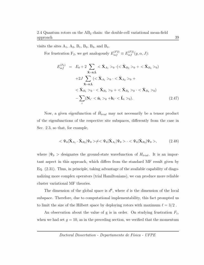
2.4 Quantum rotors on the AB2 chain: the double-cell variational mean-fieldapproach 39
visits the sites A1, A2, B1, B2, B3, and B4.
For frustration F2, we get analogously E(F2)mf ≡ E
(F2)mf (g, α, J):
E(F2)mf = E0 + 2
∑
X=n,L
< XA1>0 ·(< XB3
>0 + < XB4>0)
+2J∑
X=n,L
(< XA1>0 · < XA2
>0 +
< XB1>0 · < XB3
>0 + < XB2>0 · < XB4
>0)
−∑
i
(Ni· < ni >0 +hi· < Li >0). (2.47)
Now, a given eigenfunction of Htrial may not necessarily be a tensor product
of the eigenfunctions of the respective site subspaces, differently from the case in
Sec. 2.3, so that, for example,
< Ψ0|XA1· XB2
|Ψ0 > 6=< Ψ0|XA1|Ψ0 > · < Ψ0|XB2
|Ψ0 >, (2.48)
where |Ψ0 > designates the ground-state wavefunction of Htrial. It is an impor-
tant aspect in this approach, which differs from the standard MF result given by
Eq. (2.31). Thus, in principle, taking advantage of the available capability of diago-
nalizing more complex operators (trial Hamiltonians), we can produce more reliable
cluster variational MF theories.
The dimension of the global space is d6, where d is the dimension of the local
subspace. Therefore, due to computational implementability, this fact prompted us
to limit the size of the Hilbert space by deploying rotors with maximum ℓ = 3/2 .
An observation about the value of g is in order. On studying frustration F1,
when we had set g = 10, as in the preceding section, we verified that the momentum
Doctoral Dissertation - Departamento de Fısica - UFPE

2.4 Quantum rotors on the AB2 chain: the double-cell variational mean-fieldapproach 40
correlation < LA1· LA2
> remained pegged at 0.25, even after the transition at
J = 2, which turns out not to be true (see below). In solving this problem, we
resorted in this section to a higher value of g (namely, g = 1000), which then
inhibited more strongly the appearance of disturbing states; however one should
notice that if much greater values of g are employed, the kinetic energy becomes
overwhelmingly dominant, and as a consequence, small changes in the correlations
tend to go unnoticed.
As before, we concentrated on the relevant quantities that can provide the in-
formation needed for the physical interpretation of the problem: namely, the MF
energy, the expectation value of the total angular momentum, and the momentum
correlations. The expectation value of the total angular momentum per unit cell
was calculated according to the formula | < L > |2 = 1/2∑
µ < L2µ >, where Lµ
(µ = x, y, z) is the respective resultant component (component sum over all the
six sites of the double-cell structure).
2.4.1 Frustration F1
In order to facilitate comparison between the QR results and those of the spin-1/2
counterpart with the same type of frustration, we present in Fig. 2.9 the phases
obtained for the spin-1/2 diamond chain[57]. The Lieb-Mattis[83] ferrimagnetic
phase (FERRI) appears when J < 0.909 (J is also used to indicate the frustration
control parameter for the spin system). In the tetramer-dimer (TD) phase, which
ensues when 0.909 < J < 2, the state is precisely the regular array of singlet
tetramers (the closed loop encompasses four spins, in which the B sites form a triplet
pair, and the spins on the A sites oppose those on the B sites, so that zero total spin
takes place), and singlet dimers (two spins within the elliptical contour) as shown in
Doctoral Dissertation - Departamento de Fısica - UFPE

2.4 Quantum rotors on the AB2 chain: the double-cell variational mean-fieldapproach 41
(a) (c)(b)
DIMER−MONOMERTETRAMER−DIMERFERRIMAGNETISM
Figure 2.9: Illustration of the ground states found for the spin-1/2 diamond chain[57]as J is increased from 0. (a) The ferrimagnetic (FERRI) state. (b) The tetramer-dimer (TD) state, where rectangles represent singlet tetramers and ellipses singletdimers. (c) The dimer-monomer (DM) state. There are two first-order phase tran-sitions: at J = 0.909 (FERRI/TD) and J = 2 (TD/DM).
Fig. 2.9 (b). Finally, the dimer-monomer (DM) state is shown in Fig. 2.9 (c) and
sets in when J > 2; it is composed of the regular array of singlet dimers and free
spins, and vanishing total spin is also expected. Because of the free spins, the DM
state is macroscopically 2N/3-fold degenerate for a chain with N sites. Furthermore,
both transitions are of first order.
In order to allow a direct comparison with our MF results for quantum rotors, we
have solved the spin-1/2 diamond chain (AB2 chain with frustration between spins
at sites B of the same unit cell) for sizes up to 28 sites, using the ED procedure with
open boundary conditions. The results are displayed as follows: the relevant correla-
tions are represented by the curves plotted in Fig. 2.10; in Fig. 2.11 (a) and (b) we
plotted respectively the energy and total-spin curves (normalized by the Lieb-Mattis
value [83]).
Examination of the correlation plots show clear correspondence with the phases
exhibited in Fig. 2.9. The phase FERRI is characterized by the following correla-
tions: < SB1· SB2
>=< SB3· SB4
>= 0.25, < SB1· SB3
>= 0.21, < SA1· SA2
>=
Doctoral Dissertation - Departamento de Fısica - UFPE

2.4 Quantum rotors on the AB2 chain: the double-cell variational mean-fieldapproach 42
0 0.5 1 1.5 2 2.5J
-0.75
-0.5
-0.25
0
0.25
(A1, A
2)
(A1, B
1)
(A1, B
3)
(B1, B
2)
(B1, B
3)
(B3, B
4)
Cor
rela
tion
Fun
ctio
ns
Figure 2.10: Spin-1/2 diamond chain: ED results for the correlation functions be-tween spins at a central cluster of a system with 28 sites. Dashed lines are guidesto the eye.
Doctoral Dissertation - Departamento de Fısica - UFPE

2.4 Quantum rotors on the AB2 chain: the double-cell variational mean-fieldapproach 43
0.5 1 1.5 2 2.5J
-20
-18
-16
-14
-12
-10
E
(a)
0 0.5 1 1.5 2J
0
0.1
0.2
0.3
0.4
0.5
0.5(
S / S
LM
)
(b)
Figure 2.11: Spin-1/2 diamond chain: ED results for the (a) average ground-stateenergy and (b) rescaled total spin of a system with 28 sites. Phase transitions occurat J = 0.88 and J = 2.0, both of first order. Dashed lines are guides to the eye.
0.18, < SA1· SB3
>= −0.15, < SA1· SB1
>= −0.36. The total spin per unit cell in
Fig. 2.11 (b) shows the Lieb-Mattis value of 0.5 throughout. The transition to the
intermediate phase TD then occurs at J = 0.88, very close to the estimated value for
the infinite chain [57]: J = 0.909. We note that in this phase the chain breaks up into
smaller units - tetramers and dimers - and quantum fluctuations within each unit do
not affect the spin correlations. Hence the correlations are just those calculated for
the TD configuration of spins in Fig. 2.9 (b): < SA1· SA2
>=< SB1· SB2
>= 0.25
(triplets), < SB3· SB4
>= −0.75 (singlets), < SA1· SB1
>= −0.5, the other correla-
tions being zero. With increasing J though, quantum fluctuations become strong
enough to disrupt the tetramer unit and a new transition to the DM phase happens
at J = 2, this point being independent of size because of the chain breakup. In
this phase correlation < SA1· SA2
> has varying nonzero values due to finite size
effects, and does not vanish as should be expected in the thermodynamic limit. On
the other hand, the B spins, which are interlocked in singlet units, are totally un-
affected. This phase, depicted in Fig. 2.9 (c), shows the final chain breakup as the
Doctoral Dissertation - Departamento de Fısica - UFPE

2.4 Quantum rotors on the AB2 chain: the double-cell variational mean-fieldapproach 44
tetramer gives way to two monomer units and another dimer, clearly indicated by
the correlations in Fig. 2.10 (J ≥ 2). The energy curve in Fig. 2.11 (a) exhibits
cusps at the transition points, typical of a first-order nature, also verified through
the discontinuities of the correlations at these points. The total spin per unit cell
in Fig. 2.11 (b) corroborates the above phase description; however in the last phase
the apparent nonzero value is a finite-size effect.
Finally, getting down to the QR AB2 chain, we display our variational MF
numerical results in Fig. 2.12 (momentum correlations) and Fig. 2.13 (energy and
total angular momentum) and we proceed to a comparative examination with re-
spect to the preceding spin results. A blow-by-blow confrontation of the correlations
in both Fig. 2.10 and Fig. 2.12 shows that the double-cell variational MF approach
is able to reproduce the three phases exhibited in Ref. [57], namely, the FERRI,
TD, and DM phases. In the FERRI phase, quantum fluctuations appear to be
equally important, causing the same correlations to deviate somewhat from calcu-
lated results for stiff momenta. A closer examination shows that, up to two decimal
digits, we have same correlations for < LB1· LB2
>=< LB3· LB4
>= 0.25, but
slightly different correlations, namely: < LA1· LA2
>= 0.22, < LA1· LB1
>= 0.46,
< LA1·LB3
>= 0.20, and < LB1·LB3
>= 0.22, for the rotor system, which should be
compared with < SA1· SA2
>= 0.18, < SA1· SB1
>= 0.36, < SA1· SB3
>= 0.16, and
< SB1· SB3
>= 0.21, for the spin system. Phase transitions occur at J = 0.68 and
J = 2, evidently of first order; in the first transition we have a lesser value (J = 0.68)
than the Lanczos result for the 28-site spin-1/2 chain (J = 0.88), and that of Ref.
[57] (J = 0.909). The momentum and spin correlations match one another, respec-
tively, in both phases: in the DM phase, correlation < LA1· LA2
> shows also an
erratic behavior similar to its spin counterpart, in other words, finite size effects are
Doctoral Dissertation - Departamento de Fısica - UFPE

2.4 Quantum rotors on the AB2 chain: the double-cell variational mean-fieldapproach 45
also at play. The minor differences in correlations in the FERRI phase, as well as in
the first transition point do not constitute a fundamental discrepancy between the
respective phase diagrams, which are endowed with the same topological features.
In Fig. 2.13 (a) the cusps in the MF energy at J = 0.68 and J = 2 also bespeak
the occurrence of these first-order transitions. Comparing the total momentum in
Fig. 2.13 (b) with the total spin in Fig. 2.11 (b), we observe similar results for the
ED calculations for the spin model, including finite-size effects in the last phase.
It is instructing to study the QR system regarding the average singlet density per
unit cell of the B momenta [59], which in our case (double-cell cluster) is calculated
directly using
< η >=1
4− 1
2(< LB1
· LB2> + < LB3
· LB4>), (2.49)
and which is displayed in Fig. 2.14. These results permit a direct comparison with
the phase diagram of Fig. 2.9, as far as the buildup of singlet pairs out of B momenta
is concerned. As is the case for spins, size effects are not important here, so that
one perceives that the number of singlets is very clearly a quantized quantity within
each phase.
2.4.2 Frustration F2
Before getting down to quantum rotors, we describe succinctly existent results[59] for
the spin-1/2 AB2 chain with the same frustration F2 pattern. The rich phase diagram
of the model was studied through DMRG, ED, and a hard-core boson model. The
phase diagram thus obtained presented three transition points. The first one is
continuous and occurs at J = 0.34 between the Lieb-Mattis ferrimagnetic phase
Doctoral Dissertation - Departamento de Fısica - UFPE

2.4 Quantum rotors on the AB2 chain: the double-cell variational mean-fieldapproach 46
0 0.5 1 1.5 2 2.5 3J
-0.75
-0.5
-0.25
0
0.25
(A1, A
2)
(A1, B
1)
(A1, B
3)
(B1, B
2)
(B1, B
3)
(B3, B
4)
Cor
rela
tion
Fun
ctio
ns
Figure 2.12: QR momentum correlations calculated by using the double-cellvariational MF approach for frustration F1. One notices the phase sequenceFERRI↔TD↔DM, with first-order transitions at J = 0.68 and J = 2. Dashedlines are guides to the eye.
Doctoral Dissertation - Departamento de Fısica - UFPE

2.4 Quantum rotors on the AB2 chain: the double-cell variational mean-fieldapproach 47
0 0.5 1 1.5 2 2.5 3J
0
1
3E
mf −
E0
(a)
0 0.5 1 1.5 2 2.5 3J
0
0.25
0.5
|<L
>|
(b)
Figure 2.13: Quantum rotors by using the double-cell variational MF results forfrustration F1: (a) the energy plot (E0 = 1962) shows cusps at the first-ordertransition points J = 0.68 and J = 2.0; (b) expectation value of the total angularmomentum per unit cell. Dashed lines are guides to the eye.
(F1) and a ferrimagnetic phase (F2) characterized by the condensation of the singlet
component of the spins at the sites B1 and B2 of the same unit cell, with transverse
critical antiferromagnetic correlations. At J = 0.445, a first-order transition to a
phase characterized by spiral and predominantly AF correlations (singlet spiral)
takes place. The number of singlets in the lattice is quantized before this transition,
but is a continuous quantity afterwards, and can be envisioned by measuring the
singlet density. Further, a continuous chain-ladder decoupling transition at J = 0.91
is observed. Above this value, the A spins present critical AF correlations following
the asymptotic behavior observed in a linear chain, with power-law decay, while the
ladder of B spins are short-range correlated with a finite correlation length, whose
value is J-dependent, and nears the two-legged-ladder configuration (decoupled chain
ladder).
As far as quantum rotors are concerned, the examination of the momentum
correlations in Fig. 2.15 reveals that the system starts out with the FERRI phase
Doctoral Dissertation - Departamento de Fısica - UFPE

2.4 Quantum rotors on the AB2 chain: the double-cell variational mean-fieldapproach 48
0 1 2 3 4J
0
0.5
1
η
Figure 2.14: Quantum rotors with frustration F1: average singlet density per unitcell for the momenta of the B sites at the same unit cell. One can make out thethree phases: FERRI, TD, and DM, as well as pertinent transitions. Dashed linesare guides to the eye.
Doctoral Dissertation - Departamento de Fısica - UFPE

2.4 Quantum rotors on the AB2 chain: the double-cell variational mean-fieldapproach 49
0 0.25 0.5 0.75 1 1.5 1.75 2 2.25 2.5J
-0.75
-0.5
-0.25
0
0.25
(A1, A
2)
(A1, B
1)
(A1, B
3)
(B1, B
2)
(B1, B
3)
(B3, B
4)
(B1, B
4)
Cor
rela
tion
Fun
ctio
ns
Figure 2.15: QR momentum correlations calculated by using the double-cell vari-ational MF approach for frustration F2. One can distinguish three major phases:FERRI, CANTED, and the decoupled AF chain ladder system, with transitionsoccurring around J = 0.35 and J = 0.75. Dashed lines are guides to the eye.
Doctoral Dissertation - Departamento de Fısica - UFPE

2.4 Quantum rotors on the AB2 chain: the double-cell variational mean-fieldapproach 50
0 0.35 0.75 1J
13
14
15
16
17
E
(a)
0 1 2 3 4J
0
0.1
0.2
0.3
0.4
0.5
|<L
>|
0.33 0.34 0.35 0.36 0.37J
0
0.1
0.2
0.3
0.4
0.5
(b)
Figure 2.16: Quantum rotors by using the double-cell variational MF results forfrustration F2: (a) energy and (b) expectation value of the total angular momentumper unit cell. The inset shows details of the phase transition around J = 0.35.Dashed lines are guides to the eye.
which is the counterpart of phase F1 of the spin system studied in Ref. [59]. The
double-cell variational MF energy plotted in Fig. 2.16 (a) exhibits a pattern quite
similar to that of frustration F1, shown in Fig. 2.11 (a). But resorting to Fig. 2.15
with the help of Fig. 2.16 (b) (total average momentum per unit cell), we can clear
up the picture: in fact, at J = 0.34 its reasonable to think that a second-order
transition takes place giving rise to a narrow transient phase that corresponds to
the phase F2 (condensation of singlet components of the spins at the sites B of the
same unit cell) for the spin system and is best visualized through the inset in the
latter figure, which shows the behavior of the total angular momentum. In this phase
the momenta of the A sites keep their ferromagnetic configuration (< LA1· LA2
>=
0.25) while the B momenta conform to a magnetic canted configuration. A first-
order transition follows at J ≈ 0.36 to a new state that should correspond to the
phase singlet spiral of the respective spin system. With respect to the momenta
at the A sites, the ferromagnetic configuration also prevails in this phase. The
Doctoral Dissertation - Departamento de Fısica - UFPE

2.4 Quantum rotors on the AB2 chain: the double-cell variational mean-fieldapproach 51
total angular momentum of the A sublattice exactly counterbalances that of the
B sublattice, so that, as it happens for the spin system, a vanishing expectation
value of the total angular momentum (spin) per unit cell occurs. Furthermore,
upon inspecting the B correlations in Fig. 2.15, this phase appears here to have
also a semiclassical canted configuration, hence the name CANTED that we use to
designate this QR phase together with the previous one. In the same manner for the
spin system [59], the additional intercell interactions produce nonquantized values of
the B momenta (see, for example, correlation < LB1· LB3
>). The nonquantization
verified in the spin system, which is a coherent superposition of singlet and triplet
configurations, may rather be seen as manifestation of the symmetry-breaking of
the invariance of the Hamiltonian under interchange of the B sites in the same cell
brought about by the additional frustration. This is also clearly verified in the
QR system. In the absence of the additional frustration, as is the the case for
frustration F1 (Fig. 2.2 (a)), this symmetry stays unscathed, so that there is no
singlet-triplet superposition: we have either a singlet or a triplet configuration per
cell, but never both simultaneously, which was already verified for both spin and
QR systems. Finally, as seen in Fig. 2.15, at J = 0.75, quantum fluctuations bring
the sudden decoupling of the chain through another phase transition with first-order
characteristics (in the spin system the transition is second-order), and the system
settles into an antiferromagnetic (AF) phase, also marked by a vanishing expectation
value of the total angular momentum per unit cell, as shown in Fig. 2.16 (b). In
this phase the frustrated AB2 chain splits into two decoupled chains, namely, an AF
linear chain (< LA1· LA2
>= −0.75) and an AF two-legged ladder (< LB1· LB2
>=
< LB1·LB3
>=< LB1·LB3
>= −0.5 and< LB1·LB4
>= 0.25); the decoupling is seen
through < LA1· LB3,4
>∼= 0. In Fig. 2.17, we show a pictorial representation of the
Doctoral Dissertation - Departamento de Fısica - UFPE

2.4 Quantum rotors on the AB2 chain: the double-cell variational mean-fieldapproach 52
(a) (c)(b)
CANTED AF−LADDER + AF−CHAINFERRIMAGNETISM
Figure 2.17: Illustration of the major QR ground states for frustration F2: (a)FERRI; (b) CANTED; (c) AF, which is composed of two decoupled 1D systems: alinear chain (A sites) and the two-legged ladder (B sites).
the three major phases FERRI, CANTED and AF. With respect to this AF phase,
our QR simulations evidently shed no light onto the criticality and short-rangedness
of the linear and two-legged ladder chains, respectively. This phase corresponds to
the decoupled chain-ladder system, which in turn has a vanishing total spin. The
first-order transition at J = 0.75 may rather be seen as a manifestation of finite-size
effects of our two-cell approach: the absence of many intermediate states preclude
a smooth transition.
The average singlet density for this frustration pattern is shown in Fig. 2.18:
the singlet number is quantized (except for the narrow interval around J = 0.36,
until the frustration reaches the value J = 0.75, wherefrom the singlet number goes
on nonquantized. We see that the QR system exhibits a four-phase pattern quite
similar to that of the respective spin system, with the nature of all but the last phase
transitions being similar in both systems. With respect to singlet quantization, we
find agreement in the first and last phases (where singlet densities 0 and 0.7 are
observed); in the intermediate phases no match is observed and again we impute this
naturally to finite size effects of our two-cell approach, which hinder a discrete one-
Doctoral Dissertation - Departamento de Fısica - UFPE

2.4 Quantum rotors on the AB2 chain: the double-cell variational mean-fieldapproach 53
by-one singlet condensation. Also, because of the additional intercell frustration, it
was not possible to form isolated singlet configurations, differently from frustration
F1.
In what follows, we provide a more detailed comparison between QR MF results
and the spin-1/2 chain, in its quantum and classical versions. The phase diagram
initially described of the spin-1/2 chain from Ref. [59] is summarized in Fig. 2.19 (a).
The spiral phase can be exposed in a clear fashion through the pitch angle q obtained
from the magnetic structure factor defined as
F (q) =1
2N
∑
j,k
< Sj · Sk > eiq(j−k), (2.50)
where N ≡ Nc (in the figure) is the number of cells, with q = 2πn/(2N), for
n = 0, 1, 2, . . .2N − 1, and Sj = A(j+1)/2, if j is odd, while Sj = B1,j/2 + B2,j/2,
if j is even, and here we are labeling the sites in a more convenient way: A1, B1l,
and B2l just denote the sites A1, B1, and B2 of the lth unit cell. In the Lieb-Mattis
phase the ferrimagnetic order is indicated by a sharp peak at q = π (a period-
2 configuration); while in the decoupled phase, in which a period-4 structure is
observed (see also Fig. 2.17), there is a peak at q = π/2. These two situations are
magnetic configurations commensurate with the lattice, while the spiral phase is
indicated by a peak at a value of q between q = π/2 and q = π. In Fig. 2.19 (a)
we display the behavior of q as a function of J for finite systems calculated through
ED and DMRG (we took advantage of previous results produced in our laboratory).
Finite size effects lead to a little shift in the transition point from the spiral phase
to the decoupled phase, even though q can be clearly used to mark the spiral phase.
Doctoral Dissertation - Departamento de Fısica - UFPE

2.4 Quantum rotors on the AB2 chain: the double-cell variational mean-fieldapproach 54
0 1 2 3J
0
0.2
0.4
0.6
0.8
η
0.33 0.340.35 0.36 0.37J
0
0.2
0.4
η
Figure 2.18: Quantum rotors with frustration F2: average singlet density per unitcell for the momentum correlations at B sites along the same rung of the ladder.The inset shows details of the phase transition around J = 0.36.
Doctoral Dissertation - Departamento de Fısica - UFPE

2.4 Quantum rotors on the AB2 chain: the double-cell variational mean-fieldapproach 55
Motivated by these results, we consider the classical model in the space spanned
by two parameters (in the approach of Sec. 2.3, one single parameter sufficed to
explain the results): a canting angle θ between the B momenta at the same cell
and the pitch angle q associated with the spiral order. The classical vectors are
accordingly written as:
Al = cos[q(2l − 1)]x + sin[q(2l − 1)]z;
B1l = cos(θ) cos(2ql)x + sin(θ)(−1)ly
+ cos(θ) sin(2ql)z, and
B2l = cos(θ) cos(2ql)x + sin(θ)(−1)l+1y
+ cos(θ) sin(2ql)z, (2.51)
with |Al| = |B1l| = |B2l| ≡ 1, while x,y and z are orthogonal unit vectors in
the three-dimensional space. Substituting these fields in the classical version of
the Hamiltonian, Eq. (2.26), we get the energy function E(q, θ) ∼ 4cosq cos θ +
J(cos 2θ+cos 2q+2cos2θ cos 2q− 2sin2θ) and minimizing this function with respect
to q and θ, we find that cos(θ) = 1 and cos(q) = π for 0 < J < (1/3), which is the
classical version of the Lieb-Mattis phase found for 0 < J < 0.34 in the quantum
Hamiltonian, for both quantum rotors (FERRI phase) and spin system (Phase F1
of Ref. [59]). For (1/3) < J < 1 we obtain
cos(θ) =
√
1 − J
2J; (2.52)
cos(q) = − cos(θ), (2.53)
which may be seen as the classical version of the CANTED phase (0.34 . J .
Doctoral Dissertation - Departamento de Fısica - UFPE

2.4 Quantum rotors on the AB2 chain: the double-cell variational mean-fieldapproach 56
0.75) and of the spiral phase (0.445 . J . 0.91) found in Ref. [59]. This phase
holds some similarities with the second phase observed for the quantum rotors in
the first single-site approach of Sec. 2.3. Finally, for J > 1 the three chains are
antiferromagnetically ordered with the B momenta lying in the y direction and the
A momenta ordered in the z direction, which is the classical analog of the decoupled
phase observed for J > 0.75 for the quantum rotors and for J > 0.91 for the spin
system [59]. Such phase does not exist in the single-site approach: it is only obtained
asymptotically (J → ∞). Therefore, the classical solution presents two critical
points: Jc1,classical = 1/3 and Jc2,classical = 1, and the transitions remain second order.
Also, the first-order transition at J = 0.36 (Jt ≈ 0.445, for the spin systems) is not
observed in the classical model. In fact, in the F2 phase[59] (0.34 . J . 0.445) the
number of singlets is quantized and the spiral peak is absent, while in the classical
model the two orders coexist for Jc1,classical < J < Jc2,classical. This classical result is
also indicated in Fig. 2.19 (a).
In Fig. 2.19 (b), we present the results of this classical interpretation for the
momentum correlations. A direct relationship with Fig. 2.15 can be established: we
have the classical counterparts of the FERRI phase (J ≤ 1/3) and the AF phase
(J ≥ 1); the CANTED phase is but a gradual continuous transition between the
FERRI and AF phases. Further, the decoupling transition in the classical model is
clearly observed at J = 1 through the dot products indicated in the figure. Finally,
we notice that when this classical approach is applied to frustration F1, the minimum
energy configuration obtained is the same as that derived through the first classical
model discussed in Sec. 2.3.
Doctoral Dissertation - Departamento de Fısica - UFPE

2.4 Quantum rotors on the AB2 chain: the double-cell variational mean-fieldapproach 57
0 0.34 0.445 0.91 1J
0
0.5
1q
/ π
Nc= 8, ED Nc= 25, DMRGClassical Model
F1 F2Singlet Spiral
D
ecou
pled
C
hain
Lad
der
(a)
0 1 / 3 1J
-1
-0.5
0
0.5
1(B
1l, B
2l); (A
l, A
l+1)
(A1l, B
1l); (A
1l, B
2l)
(Bil, B
i, l+1)
(b)
Dot
Pro
duct
s
Figure 2.19: (a) Pitch angle for the quantum spin-1/2 model calculated through ED,DMRG, and for the minimum energy configuration of the classical vector model withtwo order parameters: q (pitch angle) and θ (canting angle). The transition pointsestimated in Ref. [59] are indicated. (b) Momentum dot products (i = 1, 2, and ldenotes the unit cell) in the minimum energy configuration of the classical vectormodel.
Doctoral Dissertation - Departamento de Fısica - UFPE

2.5 Summary and conclusions 58
2.5 Summary and conclusions
In dealing with quantum rotors placed at the sites of an AB2 chain we resorted
to a cluster variational MF theory implemented via two distinct approaches, which
yielded different results. First, we learned that the size of the Hilbert space could be
considerably reduced without affecting results, with the proviso that the rotor states
should be kept possibly nearest (ℓ = 1/2)-momentum states. Our main goal was
then to attempt to freeze the QR momentum tower at the least value of ℓ and so be
able to trace a paralell between rotor and spin-1/2 systems. That was attained by
increasing the importance of the kinetic energy term in the Hamiltonian (by setting
relatively high values of the coupling g), and a judicious choice of the Hilbert space,
whenever needed. This was a most important fact for the computations in multiple-
cell clusters that were to be performed in the second approach, where processing
capacity is a crucial limiting factor.
In the first approach the natural single-site MF theory was developed. A two-
phase pattern was produced with the phase transition between them being of second
order for M = 0 and of first order for M = 1. For J ≤ 1, the Lieb-Mattislike phase
typical in the spin-1/2 system arose, and for J ≫ 1, we observed the decoupling
of the system, where the momenta on the A sites tend to become uncorrelated
with the momenta on the B sites, which in turn formed singletlike pairs, while the
decoupling of the A sites was a salient feature laid bare by this approach, much like
the dimer-monomer phase in Ref. [59]. A classical interpretation was laid down
that conformed to our QR numerical findings, inclusively showing how the fixed
coupling of momentum and position turns the second-order transition into a first-
order one within certain scenarios: in this case when M = 1. With the benefit of
hindsight it was obvious that the results would be classical: in this methodology
Doctoral Dissertation - Departamento de Fısica - UFPE

2.5 Summary and conclusions 59
we dealt but with averages of quantum observables. Therefore, we were not able to
provide a reasonable quantum picture that could relate to the known behavior of the
corresponding quantum AB2 chain. Furthermore, treated this way the system was
not able to essentially tell apart frustration F1 from frustration F2 and this alone
constituted a major setback. So, all this was a reminder that the main goal of our
work still remained to be achieved.
In our last step, we then improved the former approach by producing a cluster
(double-cell) variational MF theory in which the trial Hamiltonian acts on the space
composed of the tensor product of the respective local subspaces of the six sites at
two neighboring unit cells. The gist of this theory stands on the important fact that
it allows the construction of the two-point correlations < Xi · Yj > between any
pairs of operators acting on sites i, j of the cluster. This afforded us the observation
of quantum features inherent in the system, as well as to distinguish between both
frustrations F1 and F2. For the construction of this more complex “system”, we
relied on the availability of processing capacity to carry out the numerical imple-
mentation. The experience acquired in the first approach through our endeavor to
optimize computations just carried over.
For frustration F1, besides the QR numerical simulation, we performed ED
on the spin-1/2 diamond chain using a system with 28 sites and calculated the
correlation functions between spin at a central cluster, as well as other relevant
physical quantities. Upon confronting with the QR results, we verified that the
QR phase diagrams obtained through numerical implementation of the double-cell
MF variational approach exhibited a sequence of phases analogous to those of the
spin chains, with phase transitions of the same nature. We therefore produced the
FERRI-TD-DM phase sequence, with first order transitions, which is in essence
Doctoral Dissertation - Departamento de Fısica - UFPE
2.5 Summary and conclusions 60
the phase diagram of Ref. [57]. The transition point FERRI-TD at J = 0.68
is somewhat displaced, but the transition point TD-DM at J = 2 was exactly
calculated by our approach.
For frustration F2, we obtained a phase diagram in good agreement with the
results of Ref. [59] on the respective spin-1/2 chains, endowed with the equiva-
lent frustration pattern: FERRI, CANTED, and AF which are associated with the
phases F1, F2/Spiral Singlet, and decoupled ladder chain, respectively, of the spin
model. Notwithstanding, the criticality of the A spins correlations manifests itself
here as an AF magnetic ordering due to finite-size effects. For the same reason, we
were not able to probe the short-rangedness of the correlation functions between
the B momenta. We also produced ED as well as DMRG results that helped us
to visualize the spiral phase in the spin system, and derived an insightful classical
interpretation.
Doctoral Dissertation - Departamento de Fısica - UFPE

Chapter 3
Ground state and thermodynamics
of alternating quantum spin chains
3.1 Introduction
In what follows, we present a brief review of the latest developments in molecular
magnetism. Although not at all biased, it is quite a partial account considering on
one hand the overwhelming extensiveness of the available literature on the subject
matter and, on the other hand, the limited time to carry out a thorough research.
Nevertheless, we drew on the most important facts and kept as close as possible to
our objectives in the present chapter.
The field of molecular magnetism has become nowadays a hot topic of research at
the frontier between chemistry and physics. Chemists bustle at research centers the
world over in their quest to sinthesize new compounds and predict their properties
on the basis of a molecular approach to the exchange phenomenon, while physicists
in turn test on one-dimensional (1D) materials the validity of phenomenological
61
3.1 Introduction 62
models. As one example of the early successes of these joint efforts we cite the
experimental proof of the Haldane conjecture [50] in a molecular chain compound
[85]. So far, the organic chemistry synthesis endeavor in this field has afforded a
great deal of original compounds with properties that are characteristic of both
magnets and organic compounds. Notwithstanding, to date and to the best of our
knowledge, molecular magnetism has not yet provided materials that can measure
up to metallic hard magnets at the high-temperature regime and thus be suitable
for use in everyday objects. Due to the fact that 1D magnetic systems are unable to
display long-range order at finite temperatures [86], one of the main lines of research
in molecular magnetism of the last three decades has therefore been driven by the
vehement quest to efficiently connect magnetic 1D chains in three-dimensional (3D)
networks in order to enhance bulk magnetism and make it observable and eventually
a viable industrial product. On the other hand, low-dimensional magnetic materials
besides continuing to represent a source of intermediate building blocks to be used
in the synthesis of such yearned-for bulk molecular-based materials are also very
interesting objects on their own.
So we will focus our review mostly on 1D or quasi-1D materials. At first, inves-
tigated compounds were regular homometallic chains in which the magnetic centers
are equally spaced along the chain [87–89]. In the meantime, work was also being
done on purely organic compounds (that is, which consist only of the light elements
H, C, N, and O) and one of the first bulk ferromagnets of this kind was discovered,
to wit p-nitrophenyl nitronyl nitroxide, abbreviated as p-NPNN [90]. Only ten years
later the first example of a genuine organic ferrimagnetic material having well de-
fined chemical and crystal structure was synthesized, viz the PNNBNO compound
[68]. Since the possibilities of synthesis in molecular chemistry are virtually limitless,
Doctoral Dissertation - Departamento de Fısica - UFPE

3.1 Introduction 63
the appearance of other interesting structures was naturally foreseeable. We speak
here of polymetallic chains, that is, those endowed with various metallic centers, dif-
ferent spatial intra- and interchain architectures, alternating interaction pathways
(superexchange), leading to different magnetic properties especially at low temper-
ature where interchain interactions begin to play a more significant role [91, 92].
Most important among these are the structurally ordered bimetallic chains of the
type (A-X-B-X-)n , where A and B are two different paramagnetic metal ions and
X is a bridging ligand. The first example of a bimetallic ferrimagnetic chain com-
pound [93, 94] was built of Mn2+ and Cu2+ ions endowed with spin 5/2 and spin
1/2, respectively, linked through a dithioxalato ligand. Bimetallic chains possess
intrachain interactions that are mostly of antiferromagnetic nature [93–101], with a
number of ferromagnetic chains also known [102–105]. This line of research is still
very active with the focus on cyano- and oxamato-bridged compounds being very
intense, mainly because of the discovery of slow relaxation of the magnetization at
low temperature in many of them; the cyano groups offer other possible interesting
features on the side, to wit redox activity, photosensitivity, or chirality [106].
The materials referred to so far are considered from the magnetic standpoint
either to be organic, that is, the spin carriers are organic entities, or inorganic
(homometallic chains), where the magnetic centers reside on metal complexes. An
intermediate synthesis approach resulted in the family of compounds of paramount
importance constituted by the metallo-organic (hybrid) chains, in which the spin
carriers are a metallic ion and an organic free radical, generally nitroxide. Spec-
imens of this novel family have also been synthesized and contributed to enrich
further the large variety of magnetic materials [92, 107–113]. The success of the
metallo-organic route chosen by several groups owes to the use of nitronyl nitroxide
Doctoral Dissertation - Departamento de Fısica - UFPE

3.1 Introduction 64
free radicals (NITR) where R stands for an alkyl (methyl, ethyl) or aromatic group
(phenyl). This organic entity has one unpaired electron carrying a spin 1/2, delo-
calized over the 5 atoms of its O-N-C-N-O fragment as shown by polarized neutron
studies on a compound of very weakly interacting nitronyl nitroxide molecules [114],
and the electronic configuration allows the radical to be coupled simultaneously to
two metallic groups. Such groups can be built of one magnetic 3d metallic ion such
as Cu, Ni, Mn or Co, surrounded by magnetic inactive bulky organic moieties like
hexafluoroacetylacetonates (hfac) [107–110, 113, 115]. The use of the NITR free rad-
ical leads preferentially to an antiferromagnetic intrachain coupling which proves to
be stronger as against the interaction in the bimetallic counterparts, except for the
case of some Cu complexes where ferromagnetic interactions are manifest. The pos-
sible cis or trans NITR-M(hfac)2 (M stands for a metallic ion) coordination scheme,
determined by the R group, can yield different architectural arrangements leading to
linear, zig-zag or helical chains endowed with different magnetic properties. Worth
mentioning are the studies by the pioneering research group around Caneschi [109]
within the rich and very important family of the Mn-NITR compounds, where the
underlying interaction is the strong antiferromagnetic coupling of the spin-1/2 rad-
icals and the spin-5/2 maganese(II) ions. Several other compounds with different R
groups, investigated by magnetometry and electron paramagnetic resonance (EPR),
were shown to present a ferrimagnetic 1D behavior.
The temperature dependence of the product of the molar magnetic susceptibil-
ity (χm) and the temperature (T ), in the mid- and high-temperature regime, for
ferrimagnetic polymers, when the intrachain interaction is antiferromagnetic, ex-
hibits a characteristic minimum, which may be considered as the signature of the
1D ferrimagnetic behavior. On the other hand, the magnetic properties in the very
Doctoral Dissertation - Departamento de Fısica - UFPE

3.1 Introduction 65
low-temperature range are influenced by interchain interactions, which can never be
totally ignored. In most cases, these interchain interactions lead to the onset of a
three-dimensional (3D) antiferromagnetic ordering with a sharp maximum of χmT
(and χm), as shown in Fig. 3.1. Let us consider now the case of the Mn-NITR
compounds. It is known that in these materials the chains are well magnetically
isolated from each other thanks to their large separation by bulky magnetically in-
active organic moieties. This ensures very weak interchain exchange interactions,
resulting in a ratio of intra- to interchain interaction that reaches several orders of
magnitude, so that the virtual isolation of the chains prompts a quite accentuated
1D behavior. But at low temperature, between 5K and 9K, these materials are
reported to exhibit bulk magnetic order, and this is imputed to a phase transition
toward a 3D long-range order consisting of a ferromagnetic ordering of the magnetic
centers, because in pure 1D compounds, long-range order is not expected at finite
temperature [86]. Altogether, it is necessary to take into account other usually ne-
glected interactions such as dipolar to justify such phase transition. Indeed, very
weak interchain dipolar interactions, reinforced by strong intrachain correlations,
can induce such a 3D long-range order [116–118]. The role of the dipolar interaction
has also been invoked to explain the 3D magnetic ordering of high spin molecular
cluster compounds [119–121]. More generally, the transition to the 3D long-range
order of 1D compounds is a very complex phenomenon and not totally understood
nowadays.
Now we digress briefly to touch upon an important development in the field
of molecular magnetism. More recently polynuclear clusters (complex molecules)
[122] and 1D chains [106] are being widely investigated for their ability to retain a
magnetic memory of purely molecular origin as well as for an assortment of interest-
Doctoral Dissertation - Departamento de Fısica - UFPE

3.1 Introduction 66
Figure 3.1: Temperature dependence of χmT for the first bimetallic chain (CuM-nDTO) [93, 94], where χm is the molar susceptibility and T is the temperature.Squares represent experimental points, and the full line is a plot of Eq. (3.35). Aminimum occurs at T = 130K. Reproduced from Seiden[141].
Doctoral Dissertation - Departamento de Fısica - UFPE

3.1 Introduction 67
ing quantum effects. These two classes of materials have been given the evocative
acronyms single-molecule magnets (SMM) and single-chain magnets (SCM), respec-
tively. The observation of slow magnetic relaxation in SMMs is now considered a
paramount achievement of molecular magnetism of the last few years. Such systems
have provided unique opportunities for the study of molecular magnetic hysteresis
[123], quantum tunneling of the magnetization [124], magnetic avalanches, that is
to say, abrupt magnetic reversals [125], and phase interference (Berry phase) [126],
which are features where slow magnetic relaxation plays an important part. As
already stated above, purely 1D systems do not exhibit any long-range ordering at
finite temperatures and so they cannot be stabilized as thermodynamic magnets in
consequence, for instance, of a ferromagnetic order. Nevertheless, as for SCMs the
possibility to observe the freezing of the magnetization, in a processs of very slow
relaxation, was predicted in the 1960s by Glauber [127], who developed the kinetic
model for a chain of ferromagnetically coupled spins showing Ising-type anisotropy.
Gatteschi and co-workers were the first to report observation of a slow magnetiza-
tion in a cobalt(II)-nitronyl-nitroxide alternating chain where the effective Ising-type
spin Seff = 1/2 of Co(II) and the isotropic S = 1/2 of the radical are antiferromag-
netically coupled [128]. This is another example of an experimental confirmation of
a brilliant theoretical prediction formulated more than four decades ago. Since then,
SCM behavior in several compounds has been observed [106, 129, 130], and a new
field of research opened up. Most recently it was discovered that one-dimensional
cobalt-radical coordination magnets have revealed an astounding facet: when 1D
units undergo a phase transition to 3D magnetic order, a very large coercivity arises
and increases so pronouncedly at low temperature as to make these materials com-
parable to the hardest magnets ever known [131, 132]. On the other hand, new
Doctoral Dissertation - Departamento de Fısica - UFPE

3.2 Theoretical models and methods 68
perspectives for storing information in a single magnetic polymer are wide open.
Also interesting physical properties other than magnetic are a proven possibility.
All in all, the physics and chemistry of these systems have become more and more
very active fields of research with a long, winding, but all the more exciting and
rewarding road to tread.
3.2 Theoretical models and methods
Almost all the systems referred to in the previous section can be well described,
insofar as they are considered 1D systems, by the quantum isotropic Heisenberg
Hamiltonian
Hex =∑
i,j
JijSi · Sj, (3.1)
where Si, Sj are spin operators at sites i and j (i 6= j) and Jij are the exchange inter-
actions between the respective spins and may be negative (ferromagnetic) or positive
(antiferromagnetic). Further studying the magnetic susceptibility, the Zeeman term
must be considered
Hzee = −µBHz
∑
i
giSzi , (3.2)
where the gi are the Lande factors associated with the Szi , the z projection of the
spin at site i. As opposed to the uniform linear chain, an alternating (binuclear,
i.e., the unit cell contains two spin carriers) chain, with only nearest-neighbor in-
teractions, is such a system where at least one of the following relations occur: i)
S2k−1 6= S2k, ii)J2k−1,2k 6= J2k,2k+1, or iii) g2k−1 6= g2k. Many a system reviewed in
the previous section, while thermodynamically behaving at the 1D regime, above
a certain usually low temperature threshold, can be well described by such alter-
Doctoral Dissertation - Departamento de Fısica - UFPE

3.2 Theoretical models and methods 69
nating spin chains. Among these materials, spin-1/2 spin-5/2 chains with isotropic
intrachain interaction and g factor have been the focus of intense research in the
past three decades. Materials of the sort, exhibiting both ferromagnetic systems
[91] as well as antiferromagnetic [93–95, 97, 99, 102, 109] have been character-
ized. Also chains with other alternating spin values [98, 103–105, 108], and systems
with both alternating spins and interactions have been reported [97, 100], as well
as systems with both alternating spins and g factors [97]. The first example of
an alternate ferromagnetic-antiferromagnetic spin-1/2 chain was announced by the
Caneschi team [107]. Furthermore, for a large number of other systems known in the
literature, the experimental evidence indicates that single-ion anisotropy is relevant
and so a finite magnetic anisotropy must be included in the model,
Han = D∑
i,j
Szi S
zj , (3.3)
where D is a coupling constant that gives the strength of the single-ion anisotropy.
So far, compounds modeled by this anisotropic Halmiltonian have been widely re-
searched and are particularly indicated as possible candidates to choose from in the
synthesis of SCMs [106]. Finally, we simply have a large class of compounds that can
be satisfactorily modeled by a fully isotropic Hamiltonian in which the three condi-
tions i, ii and iii above are just equalities [89, 90]. To proceed with our discussions,
we will write Eq. (3.1) in such a way as to become easy to specialize in a quantum
linear chain made up of two sublattices, with a uniform exchange interaction, which
may be either positive (antiferromagnetic) or negative (ferromagnetic):
HsS =N−1∑
i
Hi, Hi = J(Si + Si+1) · si, (3.4)
Doctoral Dissertation - Departamento de Fısica - UFPE

3.2 Theoretical models and methods 70
for a chain with N [s,S] cells.
When s = S we fall back to the totally isotropic and uniform Heisenberg spin
chain. So far, this model, as it is, for N → ∞, has been analytically intractable.
A closed-form solution has been provided only in the classical limit, when S → ∞[133]. So, when the spins are large enough, this method may be applied as was
the case of a spin-5/2 chain, with some modifications [89]. A limiting behavior
may be established from numerical results worked out on finite closed forms (rings)
extrapolated in order to yield the thermodynamic limit (N → ∞). This approximate
approach was first used by Bonner and Fisher [134], for the S = 1/2 chain and
later on extended to chains with arbitrary quantum spin numbers [135]. The only
limitation of this model is the storage and processing capacitiy of the available
computers. Therefore, other recourses have been sought in the quest to estimate
the behavior in the infinite chain limit. Among early efforts in this field of endeavor,
we cite spin-wave theory [136, 137], high-temperature series expansions [138], and
Green’s functions approaches [139].
With respect to alternating chains, i.e., chains made up of unequal sublattices
(s 6= S), the first attempt at finding a closed form for the susceptibility χ was carried
out by Blote [140], who set one of the spin quantum numbers infinite (i.e., it could
be treated classically). However, in his calculations he neglected the contribution of
the quantum sublattice vis-a-vis the classical one, thus rendering his procedure un-
able to take into account the experimental results. In 1981, Verdaguer and Gleizes
discovered the first bimetallic chain [93, 94], and this stimulated extensive theoreti-
cal research in the area. The compound CuMn(S2C2O2)2 ·7.5H2O (CuMnDTO) was
made up of two different paramagnetic ions, Cu2+ and Mn2+, structurally ordered
in an alternating manner and bridged by a polyatomic dithioxalato anion ligand
Doctoral Dissertation - Departamento de Fısica - UFPE

3.2 Theoretical models and methods 71
- showing the pattern of a regular -Cu-Mn-Cu-Mn- alternating spin-1/2 spin-5/2
chain. Motivated by the failure of previous models to explain the properties of the
new compound, Seiden [141] set about solving analytically the magnetic suscepti-
bility of the [1/2, S] chain, where S is large enough to be considered classical. So
far, this simple model has been a valuable tool in the research of new materials
[97, 108, 109, 112, 115, 122], besides constituting another interesting example of the
interplay between the experimental and theoretical assembly lines.
In the context of pure quantum methods, alternating-spin Heisenberg chains
were initially approached by numerical diagonalization [142]. Further investiga-
tions were carried through with the use of the powerful techniques of density-matrix
renormalization group [143, 144] and quantum Monte Carlo methods [145, 146] in
an attempt to clear up dual features of ferrimagnetic excitations. The conventional
antiferromagnetic spin-wave formalism [136, 137] has been modified, on the one
hand by following the Takahashi prescription [147], which was orginally proposed
for ferromagnets, and then for 2D antiferromagnets [148], while on the other hand
with the introduction of a slightly different approach [149]. The finite-temperature
Lanczos method (FTLM) [150] - which is based on the Lanczos diagonalization tech-
nique and random sampling - has also become a very useful tool in the evaluation
of both static and dynamical quantities in small many-body quantum systems. We
will take advantage of such method in this chapter in a similar manner we did ED
previously.
Doctoral Dissertation - Departamento de Fısica - UFPE

3.3 Static properties of an alternating isotropic chain of quantum spins 1/2 andclassical spins 72
3.3 Static properties of an alternating isotropic
chain of quantum spins 1/2 and classical spins
We now provide an overview of the article by Seiden [141], which as stated before,
has been taken advantage of in the determination of the coupling constant J , as an
indicator of the dimensionality as well as the overall behavior of the investigated
materials (for which one sublattice spin can be treated as a classical vector) in the
mid- and high-temperature ranges. We proceed then with the main purpose of
retrieving the analytical expresssion of the magnetic susceptibility, which will later
be recalled in this chapter, but also with a didactical mind so that, when deemed
necessary, we try to clarify a couple of passages here and there in the paper.
The Hamiltonian was already given in Eq. (3.4), and in Fig. 3.2 (a) we provide
a depiction of the alternating chain (sS chain) in question, illustrating the ground
state, which according to the Lieb-Mattis theorem [83] possesses a net spin 2 per
unit cell. In what follows, the spins si will be treated as quantum operators, with
s = 1/2, whereas the spins Si will be considered vectors of length S. As a result,
each si is coupled only with its two classical next neighbors Si and Si+1, so that
all the Hi commute. This is the great advantage of interspersing classical vectors
throughout the chain, in between the quantum spins, allowing for a simple expression
of the partition function below, from which quantities of interest can be analitically
derived.
Doctoral Dissertation - Departamento de Fısica - UFPE

3.3 Static properties of an alternating isotropic chain of quantum spins 1/2 andclassical spins 73
3.3.1 Free energy
One sets about calculating the free energy. The partition function is given by
Z =
(
2S + 1
4π
)N ∫
dΩ1 . . . dΩN z1,2z2,3 . . . zN−1,N , (3.5)
with
zi,i+1 = exp
(−βJSi,i+1
2
)
+ exp
(
βJSi,i+1
2
)
, (3.6)
and
Si,i+1 = Si + Si+1, Si,i+1 = |Si,i+1| = S√
2(1 + cos θi,i+1), (3.7)
where θi,i+1 is the angle formed by Si and Si+1, and we consider the z direction as
that of Si +Si+1. There are N classical spins (which amounts to say N cells) and N-1
quantum spins: open boundary conditions, where each quantum spin is surrounded
by two classical vectors. In Eq. (3.6), one summed over the quantum degrees of free-
dom (sz = −1/2,+1/2) projected on the zi direction. In Eq. (3.5), the integration
over the classical degrees of freedom was already performed in dS, where the coor-
dinate S was assumed to take on 2S + 1 discrete values (semi-quantum approach),
while remaining N angular integrations to be carried out (dΩi = sin θi dθi dφi). 4π
is just a normalization constant related to the solid angle of the entire sphere.
The next step consists in developing Eq. (3.6) in a series of Legendre polyno-
mials:
zi,i+1 = z(θi,i+1) =∞
∑
l=0
alPl(cos θi,i+1). (3.8)
The above polynomials, involving an angle between two vectors (θi,i+1), can be
farther developed in terms of the individual angles (θi and θi+1) by using the addition
Doctoral Dissertation - Departamento de Fısica - UFPE

3.3 Static properties of an alternating isotropic chain of quantum spins 1/2 andclassical spins 74
theorem for spherical harmonics
Pl(cos θi,i+1) =4π
(2l + 1)
m=l∑
m=−l
Y ∗l,m(θi, φi)Yl,m(θi+1, φi+1). (3.9)
Upon using the normalization and orthogonality conditions
∫ 2π
0
dφ
∫ π
0
Y ∗l′,m′(θ, φ)Yl,m(θ, φ) = δl,l′δm,m′ , (3.10)
the partition function for a finite chain (with N classical vectors) can be evaluated,
namely:
Z = (2S + 1)N
∞∑
l=0
aN−1l
(2l + 1)N−1. (3.11)
and for an open and infinite chain (N → ∞), one gets finally the mathematically
rigorous result
Z = (2S + 1)NaN−10 , (3.12)
from which the desired expression for the free energy can be derived, which then
reads
F = − 1
βlogZ, (3.13)
where the term a0 must yet be calculated. This will be done in a short while.
3.3.2 Two-spin correlations
There are three types of correlations to be calculated, defined below so as to cohere
with the rotational invariance of the Hamiltonian in Eq. (3.4), namely
Doctoral Dissertation - Departamento de Fısica - UFPE
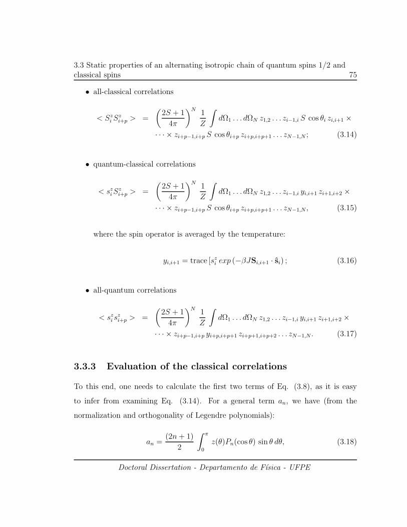
3.3 Static properties of an alternating isotropic chain of quantum spins 1/2 andclassical spins 75
• all-classical correlations
< Szi S
zi+p > =
(
2S + 1
4π
)N1
Z
∫
dΩ1 . . . dΩN z1,2 . . . zi−1,i S cos θi zi,i+1 ×
· · · × zi+p−1,i+p S cos θi+p zi+p,i+p+1 . . . zN−1,N ; (3.14)
• quantum-classical correlations
< sziS
zi+p > =
(
2S + 1
4π
)N1
Z
∫
dΩ1 . . . dΩN z1,2 . . . zi−1,i yi,i+1 zi+1,i+2 ×
· · · × zi+p−1,i+p S cos θi+p zi+p,i+p+1 . . . zN−1,N , (3.15)
where the spin operator is averaged by the temperature:
yi,i+1 = trace [szi exp (−βJSi,i+1 · si) ; (3.16)
• all-quantum correlations
< szi s
zi+p > =
(
2S + 1
4π
)N1
Z
∫
dΩ1 . . . dΩN z1,2 . . . zi−1,i yi,i+1 zi+1,i+2 ×
· · · × zi+p−1,i+p yi+p,i+p+1 zi+p+1,i+p+2 . . . zN−1,N . (3.17)
3.3.3 Evaluation of the classical correlations
To this end, one needs to calculate the first two terms of Eq. (3.8), as it is easy
to infer from examining Eq. (3.14). For a general term an, we have (from the
normalization and orthogonality of Legendre polynomials):
an =(2n+ 1)
2
∫ π
0
z(θ)Pn(cos θ) sin θ dθ, (3.18)
Doctoral Dissertation - Departamento de Fısica - UFPE

3.3 Static properties of an alternating isotropic chain of quantum spins 1/2 andclassical spins 76
from which derive
a0 =1
2
∫ π
0
z(θ) sin θ dθ and a1 =3
2
∫ π
0
z(θ) cos θ sin θ dθ. (3.19)
Noting that cos θ/2 = [(1 + cos θ)/2)]1/2, with the appropriate change of variables
(βJS cos θ/2 = u), and by using the formulas from elementary calculus
∫
u cosh(u) du = u sinh(u) − cosh(u),∫
u3 cosh(u) du = (u3 + 6u) sinh(u) − (3u2 + 6) cosh(u), (3.20)
one finds finally:
a0 = 4(x−1 sinh(x) − x−2 cosh(x) + x−2),
a1 = 12[(x−1+ 12x−3) sinh(x) − (5x−2+ 12x−4) cosh(x) − x−2 + 12x−4], (3.21)
where x = βJS = JS/kBT . Now, with the value of a0 at hand, the free energy can
then be calculated as a by-product.
To calculate the classical correlations as prescribed by Eq. (3.14), we note
that the integrals over dΩ1 . . . dΩi−1 as well as those over dΩi+p+1 . . . dΩN can be
factored off (they contribute a factor of 4π(4πa0)N−p−1 which cancel out with an
equal contribution coming from 1/Z outside of the integral). To accomplish our
task we have to calculate now the correlated integrals (dΩi+1 . . . dΩl+p, whereto we
resort to a technique used by Fisher [133]: The angles θi and θi+p are polar angles
referred to the z axis. By using Si+p−1 as polar axis, with Si defining the reference
Doctoral Dissertation - Departamento de Fısica - UFPE

3.3 Static properties of an alternating isotropic chain of quantum spins 1/2 andclassical spins 77
plane for φi+p, we have
cos θi+p = cos Θi+p cos θi+p−1 + sin Θi+p sin θi+p−1 cos(Φi+p − φi+p−1), (3.22)
where Θi+p is the angle between Si+p and Si+p−1. Upon integration only the first
term in Eq. (3.22) survives due to < cos Φi+p >≡ 0, and so we get
< cos θi+p >=< cos Θi+p > < cos θi+p−1 >=< cos θi+p−1 > < cos θ >, (3.23)
where Θi+p is turned into the integration variable θ. By repeating the procedure
for cos θi+p−1, we can then infer a simple recurrence relation. Thus, by means
of Eq. (3.23), we perform the last part of the integration, yielding a factor of
(4π)p(a1/3)pS2, which divided by the rest factor (4πa0)p coming from 1/Z (outside
the integral) gives finally (a1/3a0)pS2. The pair correlation function is defined here
so that < Szi S
zi+p >= 1
3< Si · Si+p > (rotational invariance), whereby a factor of
1/3 must be brought into the final result:
< Szi S
zi+p >= δp S
2
3, (3.24)
with
δ =a1
3a0. (3.25)
Doctoral Dissertation - Departamento de Fısica - UFPE

3.3 Static properties of an alternating isotropic chain of quantum spins 1/2 andclassical spins 78
3.3.4 Evaluation of correlations comprising quantum spins
One uses the basis spanned by the eigenstates of sz (sz|m >= m|m >) to evaluate
the expression of Eq. (3.16), resulting in
y =∑
m
∑
µ
< m|µ >< µ| exp (−βJS · s) |µ >< µ|m >, (3.26)
where |µ > are the eigenstates of the projection of s on S, and < m|µ > are the
matrix elements of the Wigner-D1/2(ψ) matrix:
D1/2(ψ) =
cosψ/2 − sinψ/2
sinψ/2 cosψ/2
and ψ is naturally the angle with the z axis. One gets straightforwardly (s = 1/2)
y = − cosψ sinh
(
βJS
2
)
; (3.27)
cosψi,i+1 =Sz
i,i+1
Si,i+1
=(cos θi + cos θi+1)
Si,i+1
. (3.28)
By expanding the following in a series of Legendre polynomials
sinh(
βJSi,i+1
2
)
Si,i+1
=∞
∑
l=0
blPl(cos θi,i+1), (3.29)
and with the aid of the calculus formula, with the same change of variables used
previously∫
u2 sinh(u) du = (u2 + 2) cosh(u) − 2u sinh(u), (3.30)
Doctoral Dissertation - Departamento de Fısica - UFPE

3.3 Static properties of an alternating isotropic chain of quantum spins 1/2 andclassical spins 79
one obtains
b0 = x−1[cosh(x) − 1],
b1 = 3[(x−1+ 4x−3) cosh(x) − 4x−2 sinh(x)+ x−1 − 4x−3]. (3.31)
Proceeding analogously to the determination of the all-classical correlations carried
out in the previous subsection and introducing
Λ = 2
(
b13a0
+b0a0
)
, (3.32)
one gets finally
< sziS
zi+p > = −Λδp−1sS
3,
< szi s
zi+p > = Λ2δp−1s
2
3, (3.33)
where p > 0. For completeness, the self-correlations are included: < szi s
zi >=
s(s + 1)/3 and < Szi S
zi >= S(S + 1)/3; the latter defined in such a manner as to
build a consistent theory.
3.3.5 Magnetic susceptibility
The susceptibility in zero field can now be calculated from the fluctuation relation
χ = βµ2B
∑
i,j
< (gS Szi + gs s
zi ) (gS S
zj + gs s
zj) >, (3.34)
where gS and gs are the g factors of the classical and quantum spins, respectively.
By using the correlations just calculated and noting that δ < 1, so that∑∞
p δp =
Doctoral Dissertation - Departamento de Fısica - UFPE
3.3 Static properties of an alternating isotropic chain of quantum spins 1/2 andclassical spins 80
δ/(1 − δ)∑∞
p δp−1 = 1/δ∑∞
p δp = 1/(1 − δ), one gets the closed form for the
magnetic susceptibility
χ=Nβµ2
B
3
[
g2SS
2
(
S + 1
S+ 2
δ
1 − δ
)
−4gSgsΛsS1
1 − δ+ g2
s
(
s(s+ 1)+2Λ2s2 1
1 − δ
)]
,
(3.35)
for a chain with N ≫ 1 cells. When J > 0, the quantity Tχ(T ) has a minimum at
a temperature Tm which is generally situated in a region where βJS < 1, a feature
which has been known to be typical of 1D ferrimagnets. At low temperatures, i.e.,
x≫ 1, or J |S|kBT
≫ 1, it is found in first order δ1−δ
= Λ1−δ
= Λ2
1−δ≈ x
4, so that
χ =Nβµ2
B
3
[
g2SS(S + 1) + g2
ss(s+ 1) +βJS
2(gSS − J
|J |gss)2
]
, (3.36)
and we note that only integer powers of the temperature are present.
To adjust Eq. (3.35) to the experimental data of Fig. 3.1, by setting gS = gs,
Seiden identified J = 59.7 and g = 1.9.
In another paper [94], Verdaguer et al., by making use of the same classical
approximation, centered on the transfer matrix technique, developed a numerical
method for the calculation of the susceptibility yielding a more precise value of the
intrachain coupling J = 43.6 (as opposed to the value of J = 59.7 found by way of
Eq. 3.35). This new approach may be viewed as a refinement of the results discussed
here, albeit not analytical.
In Fig. 3.2 (b), we sketch the alternating chain (ssS chain), with the zero-
field ground state explicitly indicated, which was used to model the compound
[Mn(NITIm)(NITImH)]ClO4, from now on indicated as MnNN, where NITIm is a
bis-chelating nitronyl nitroxide ligand, that was studied in the work by Fegy et al.
Doctoral Dissertation - Departamento de Fısica - UFPE

3.3 Static properties of an alternating isotropic chain of quantum spins 1/2 andclassical spins 81
[111]. This chain can be expressed by a Hamiltonian of the form
HssS = J
N−1∑
l=1
sl · (Sl + Sl+1) + J′
N∑
l=1
Sl · s′
l, (3.37)
where sl and s′
l are spin-1/2 variables (nitronyl nitroxide radical) and Sl are spin-
5/2 variables (ion MnII). By using this semiclassical approximation, where the
spin-5/2 are treated as classical vectors, they calculated a closed expression for the
susceptibility in an analogous way, namely
χ =Nβg2µ2
B
3[S2 + s(s+ 1) + s′(s′ + 1) − St+
1
1 − δ(−4SΛ + 2Λ2 + 2Λt) +
δ
1 − δ
(
2S2 − 2St+t2
2
)
], (3.38)
where t = tanh(J ′βs), with δ and Λ as defined previously..
In the next section we will apply FTLM [150] to finite-size chains described by
the Hamiltonians given by Eqs. (3.4) and (3.37), for the case where s = s′ = 1/2 and
S = 5/2. The results so produced will be put together in the context of experimental
data [93, 94, 111] as well as calculations from other theoretical approaches, namely,
the semiclassical magnetic susceptibility expressed by Eqs. (3.35) and (3.38) and
spin-wave results [143, 147, 149, 151] and then comparisons will be drawn. Thus a
brief review of FTLM is in order. This is provided in Appendix A.2.
Doctoral Dissertation - Departamento de Fısica - UFPE

3.3 Static properties of an alternating isotropic chain of quantum spins 1/2 andclassical spins 82
J
J
J´
(a): sS chain
(b): ssS chain
Figure 3.2: Schematic representation of the Hamiltonian and ground-state magneticorder of the (a) sS and (b) ssS alternating chains. In Seiden’s paper [141] the largerspin (longer arrow) is a classical quantity, the other one being quantum.
Doctoral Dissertation - Departamento de Fısica - UFPE

3.4 Alternating spin-1/2 spin-5/2 ferrimagnetic chains - ground state andthermodynamics 83
3.4 Alternating spin-1/2 spin-5/2 ferrimagnetic
chains - ground state and thermodynamics
We now present ED and FTLM results for the ground state and thermodynamic
functions. Whenever possible, we bring together pertinent experimental data as
well as results from other theoretical approaches for the sake of comparison. From
now on, differently from the previous subsection, the number of magnetic sites in the
chain will be indicated with the letter N, so that the sS chain has N/2 cells and the
ssS chain, N/3 cells. To avoid confusion, the number of cells will be appropriately
indicated by Nc.
3.4.1 Ground states - ED results
One-magnon bands
In Figs. 3.3 and 3.4 we display one-magnon bands for the sS and ssS chains, respec-
tively. For the sS chain, where we have set J = 44.8K (see Subsection 3.4.2, Fig.
3.10), the ground state of a system with Nc cells is found to be ferrimagnetic with
total spin SG = 2Nc. The bands show that there is a gapless excitation to a state
with spin SG − 1 and a gapped one to a state with spin SG + 1. Testing for various
sizes we can infer the size of the gap ∆, and so we have arrived at ∆ = 4.90J . In the
respective figure appear also plots of the dispersion relations from the calculations
Doctoral Dissertation - Departamento de Fısica - UFPE

3.4 Alternating spin-1/2 spin-5/2 ferrimagnetic chains - ground state andthermodynamics 84
of non-interacting spin waves of Ref. [143], for s1 = 1/2 and s2 = 5/2, namely
ω1q = J(−s1 + s2) + ωq,
ω2q = J(s1 − s2) + ωq,
ωq = J√
(s1 − s2)2 + 4s1s2 sin2(q/2). (3.39)
The acoustical mode (gapless) calculated through both approaches superimpose,
whereas the optical mode (gapped) does not: the non-interacting spin-wave disper-
sion is different and has a smaller gap, as is often the case with other mixed-spin
systems. See, for example, Ref. [151].With respect to the ssS chain, where we have
set J ′/J = 1.7 (see Subsection 3.4.2, Fig. 3.11), similar results were produced, with
a lesser value for the gap (∆ = 3.88J). We have not found in the literature calcu-
lations of the dispersion relations for this chain topology, which could be taken for
referral.
Magnetization
In Fig. 3.5 we show the magnetization per cell for the sS chain as a function of the
applied magnetic field. The first plateau ends at a field bc = gµBBc/J ≈ 4.9, which
corresponds to the gap of the first antiferromagnetic excitation already shown in
Fig. 3.3. This corresponds to a huge field that must be turned on to bridge this
gap (Bc ∼ 150T ). To reach the saturation point, we need a very high field BS =
JbS/gµB ∼ 200 T. In order to estimate the thermodynamic-limit transition pathway,
we have used various chain sizes. Next we exhibit in Fig. 3.6 the magnetization of
the ssS chain, which conveys a similar pattern of behavior. The first plateau ends
at bc = gµBBc/J ≈ 3.9, which is the spin-wave gap height of Fig. 3.4.
Doctoral Dissertation - Departamento de Fısica - UFPE

3.4 Alternating spin-1/2 spin-5/2 ferrimagnetic chains - ground state andthermodynamics 85
0 1 2 3q
0
1
2
3
4
4.9
6
[E(S
z ,q)-
EG
S] / J
N=24N=20
0 0,05 0,1
1 / N
4,904
4,905
4,906
∆
Figure 3.3: One-magnon bands of the sS chain. Full lines are spin-wave results fromRef. [143], while dashed lines are guides to the eyes. Sz = SG−1 for the lower band,while Sz = SG+1 for the upper one. Inset: Size dependence of the antiferromagneticgap ∆, which is estimated to be ∆ = 4.9046J in the thermodynamic limit.
Doctoral Dissertation - Departamento de Fısica - UFPE

3.4 Alternating spin-1/2 spin-5/2 ferrimagnetic chains - ground state andthermodynamics 86
0 1 2 3q
0
1
2
3
3.9
5
[E(S
z ,q)-
EG
S] / J
N=18N=21
0 0,05 0,1
1 / N
3,88
3,89
3,9
3,91
∆
Figure 3.4: One-magnon bands of the ssS chain with J′
= 1.7J . Dashed lines areguides to the eyes.Sz = SG − 1 for the lower band, while Sz = SG + 1 for the upperone. Inset: Size dependence of the antiferromagnetic gap ∆, which is estimated tobe ∆ = 3.88J in the thermodynamic limit.
Doctoral Dissertation - Departamento de Fısica - UFPE

3.4 Alternating spin-1/2 spin-5/2 ferrimagnetic chains - ground state andthermodynamics 87
0 1 2 3 4 bc
bS
7B / (J / gµ
B)
2/3
1
M /
Msa
t
N = 8N = 10N = 12N = 16
Figure 3.5: Magnetization per cell M normalized by its saturation value Msat =3gµB as a function of applied magnetic field B in units of J/gµB at T = 0 for the sSchain. We have set J = 44.8K (see Subsection 3.4.2, Fig. 3.10). The first plateauends at bc = gµBBc/J ≈ 4.9 which implies that Bc ∼ 150 T. On the other hand,the saturation field BS = JbS/gµB ∼ 200 T.
Doctoral Dissertation - Departamento de Fısica - UFPE

3.4 Alternating spin-1/2 spin-5/2 ferrimagnetic chains - ground state andthermodynamics 88
0 1 2 bc
bS
7
B / (J / gµB)
0
3/7
5/7
1
M /
Msa
t
N = 9N = 12N = 15N = 18
Figure 3.6: Magnetization per cell M normalized by its saturation value Msat =3.5gµB as a function of applied magnetic field B in units of J/gµB at T = 0 for thessS chain with J
′
= 1.7J (see Subsection 3.4.2, Fig. 3.11). The first plateau endsat bc = gµBBc/J ≈ 3.9 which implies that Bc ∼ 400T . On the other hand, thesaturation field BS = JbS/gµB ∼ 600T .
Doctoral Dissertation - Departamento de Fısica - UFPE

3.4 Alternating spin-1/2 spin-5/2 ferrimagnetic chains - ground state andthermodynamics 89
0 10 20 30 40 50 60
B ( 103 G )
0
4
8
12
16
20
24
M (
103 c
m3 m
ol-1
)
FTLM ExperimentalQuantum Paramagnet
0 500 1000150020000
10
20
30
T = 4.2 KT = 0
Figure 3.7: Magnetization per mol for the sS chain as a function of the appliedmagnetic field B for T = 4.2 K. Experimental data of the compound CuMnDTOfrom Ref. [94, 141]. FTLM for a system with N = 16, J = 44.8 K and g = 1.93.Quantum paramagnet: fitting of the FTLM data to the magnetization per mol of aquantum paramagnet (Brillouin function) with total spin S. Taking g = 1.93, thebest fit implying S = 15.8. The inset serves the purpose of showing how the finitetemperature modifies the field-induced Lieb-Mattis ferrimagnetic ground state.
3.4.2 Thermodynamic quantities
The study of the thermodynamic functions is carried out through the numerical
implementation of the FTLM on chains of finite size. Unless expressly indicated
otherwise, we use in our FTLM computations M = 50 for both sS and ssS chains,
while setting R = 40000 for the former and R = 50000 for the latter. Periodic
boundary conditions were used. When not explicitly shown, we have deemed con-
venient to set kB = 1 throughout this section.
Doctoral Dissertation - Departamento de Fısica - UFPE

3.4 Alternating spin-1/2 spin-5/2 ferrimagnetic chains - ground state andthermodynamics 90
0 0,25 0,5B / (J/gµ
B)
0
0,2
0,4
0,6
0,8
1
M /
M (
T =
0)
FTLMQuantum Paramagnet
0 2 4 60
0,5
1
1,5
23.5/1.5
Figure 3.8: FTLM results for the magnetization normalized by its value at T =0(M(T = 0) = 1.5 per cell) for the ssS chain as a function of the normalized appliedmagnetic field at T = 0.1J . The system size is N = 18. Quantum paramagnet:fitting of the FTLM data to the expected curve for a quantum paramagnet (Brillouinfunction) with total spin S, the best fit implying S = 8.74. The inset serves thepurpose of showing how the finite temperature modifies the field-induced Lieb-Mattisground state.
Doctoral Dissertation - Departamento de Fısica - UFPE

3.4 Alternating spin-1/2 spin-5/2 ferrimagnetic chains - ground state andthermodynamics 91
Magnetization
In Fig. 3.7 we show the FTLM results of the molar magnetization as a function of
the applied magnetic field for T = 4.2K. The experimental data [94, 141] for the
compound CuMnDTO are also included. A good agreement between both results is
observed. We have also contemplated the magnetization M(B, T ) of the quantum
paramagnet given by the Brillouin function, namely
BJ(x) =1
S
(S + 1/2) coth [(S + 1/2)x] − 1
2coth(
x
2)
,
M(B, T ) = NgµBJBJ(x), (3.40)
where x = gµBB/kBT , and B is the applied magnetic field. Eq. (3.40) is also plotted
and fitted to the FTLM data. Taking g = 1.93, and chain size N = 16, we attain
the best fit by setting S = 15.8. This means that the spins are stirred thermally, so
that the total spin is less than its field-induced Lieb-Mattis ferrimagnetic ground-
state value, that is, SLieb = 16. We then envision an ensemble formed by insulated
spin-15.8 units in a thermal bath, i.e., a quantum paramagnet, no less. We have
proceeded in the same way relative to the ssS chain and display the results in Fig
3.8: a good fit is verified by using S = 8.74, which because of ensuing thermal
fluctuations is less than the total spin SLieb = 9 of the field-induced Lieb-Mattis
ferrimagnetic ground state.
Magnetic susceptibility
In Fig. 3.9 we present the product of the susceptibility per site by the temperature
as a function of the temperature - (χT × T ) - for the sS chain. The chain size is
N = 16. The characteristic 1D ferrimagnetic minimum takes place at Tm = 2.9J ,
Doctoral Dissertation - Departamento de Fısica - UFPE

3.4 Alternating spin-1/2 spin-5/2 ferrimagnetic chains - ground state andthermodynamics 92
0 2 4 6 8 10T / J
0
1
2
3
4
5
6
χT /
g2 µ B
2 2 2,2 2,4 2,6 2,8 3
T / J-0,15
-0,1
-0,05
0
0,05
0,1
(J /
g2 µ B
2 )d(χ
T)
/ dT
Figure 3.9: Product of the susceptibility per site χ and the temperature T for thesS chain with N = 16. In the inset we present the derivative of this curve in thetemperature range in which its minimum, Tmin = 2.9J , is found.
Doctoral Dissertation - Departamento de Fısica - UFPE

3.4 Alternating spin-1/2 spin-5/2 ferrimagnetic chains - ground state andthermodynamics 93
0 100 200T(K)
0
2
4
6
8
10
12
χ mT(c
m3 K
mol
-1)
ExperimentalSemiclassical FTLM
Figure 3.10: Product of the molar susceptibility χm and temperature T as a functionof T for the sS chain. Experimental data for the compound CuMnDTO from Ref.[141]. Semiclassical susceptibility according to Eq. (3.35): J = 59.7 K, S = 2.5 andg = 1.9. FTLM results for a system with N = 16, the best fit to the experimentaldata implies J= 44.8 K and g = 1.90.
Doctoral Dissertation - Departamento de Fısica - UFPE

3.4 Alternating spin-1/2 spin-5/2 ferrimagnetic chains - ground state andthermodynamics 94
100 150 200 250 300T
2,8
2,9
3
3,1
3,2
χ mT
(cm
3 K m
ol-1
)
1.51.72.0Experimental
(a)
0 2 4 6 8 10T / J
0,6
0,8
1
1,2
1,4
1,6
1,8
2
χT /
(g2 µ Β
2 )
1 1,5 2 2,5 3
T / J
-0,2
-0,1
0
0,1
(J/g
2 µ Β2 )d
(χT
) / d
T
(b)
Figure 3.11: Product of the susceptibility per site χ and the temperature T for thessS chain with N = 18. (a) The numerical data, for the indicated values of J
′
/J ,are compared with the experimental data for the compound MnNN from Ref. [111]by arbitrarily defining J = 100K, in order to enhance graph readability. (b) χTfor J
′
= 1.7J and its derivative, shown in the inset. The minimum of this curve isfound at Tmin = 1.7J .
calculated in the way indicated in the inset, through the numerical derivative. Then
in Fig. 3.10 we put together our FTLM results, the semiclassical susceptibility
(Eq. (3.35)), and the experimental data [94, 141] for the compound CuMnDTO.
By using Eq. (3.35), Seiden estimated J = 59.7K and g = 1.9. The best fit of
our FTLM results to the experimental data yielded J = 44.8K and g = 1.90. Our
estimate of J is closer to the one obtained through other numerical approach [94] to
which we have already referred in Subsection 2.3.5. The evaluation of J is made by
using the value of Tmin = 130K, which indicates the minimum of the experimental
curve. We see that both FTLM and semiclassical approaches agree with experiment
in the mid- and high-temperature regimes. This is the regime where the interchain
interactions can be considered negligible. Otherwise, and with the concurrence of
other factors, the system seems to evolve toward a 3D long-range ferromagnetic
Doctoral Dissertation - Departamento de Fısica - UFPE

3.4 Alternating spin-1/2 spin-5/2 ferrimagnetic chains - ground state andthermodynamics 95
0 50 100 150 200 250 300 350 400T (K)
0
5
10
15
20
χ mT
(cm
3 K m
ol-1
)
ExperimentalSemiclassical FTLM
Figure 3.12: Product of the molar susceptibility χm and temperature T as a functionof T for the ssS chain. Experimental data of the MnNN compound from Ref. [111].Semiclassical susceptibility according to Eq. (3.38): J = 144 K, J
′
= 248 K, S = 2.5and g = 2.0. FTLM results for a system withN = 18, the best fit to the experimentaldata implies J = 150 K and J
′
= 255 K, while g(= 2.0) is not taken as a fittingparameter.
Doctoral Dissertation - Departamento de Fısica - UFPE

3.4 Alternating spin-1/2 spin-5/2 ferrimagnetic chains - ground state andthermodynamics 96
ordering, and therefore, we are unable to push further with our simple 1D model in
the quest of explaining experimental data, for this material and the like.
Next, in Fig. 3.11. we show the temperature dependence of χT for the ssS chain.
The ratio J ′/J nearest the experimental data is determined as indicated in Fig. 3.11
(a). The ubiquitous characteristic minimum is estimated as in the previous case and
is shown in Fig. 3.11 (b). Next we present in Fig. 3.12 the FTLM and semiclassical
results (Eq. (3.38)), derived ad hoc for this chain, alongside the experimental data
of the MnNN compound. The FTLM results stray from the other two below a
certain temperature. We cannot but impute to finite-size effects the discrepancy of
the FTLM procedure, a hindrance which is unfortunately difficult to be bypassed
by means of the present technique alone, because of machine limitations.
Specific heat
In Fig. 3.13 we show the specific heat at zero applied field for both sS and ssS
chains. The outstanding features are the double peaks, which are reminiscent of
the Schottky effect [149, 151, 152]. This phenomenon is actually observed in the
laboratory [96]. We also drew the respective Schottky specific heat curves. We
see that the ssS and Schottky curves fit together nicely, and furthermore the peak
height that comes out agrees with the spin-wave band gap - the Schottky energy
gap δ ≈ 4.1J being just a bit over the expected value, to wit ∆ = 3.9j. But we seem
to have a problem with respect of the fit to the sS chain: we do not get so good an
adjustment as with the other chain. To verify if a reasonable adjustment was ever
possible, we then worked based on the faint premise that the first left-hand peak
somehow strongly influences the higher one, whereas this does not happen with the
ssS chain, whose first peak is almost nonexistent, appearing as a mere inflection
Doctoral Dissertation - Departamento de Fısica - UFPE

3.4 Alternating spin-1/2 spin-5/2 ferrimagnetic chains - ground state andthermodynamics 97
0 2 4 6 8 10T / J
0
0.1
0.2
0.3
0.4
C /
Nk B
ssSsS
Figure 3.13: Specific heat per site as a function of temperature T for sS and thessS, with J
′
= 1.7J , chains. The full lines are the respective Schottky specific heats(Eq. (3.41)). Dashed lines are guides to the eye.
point. We finally opted to calculate the specific heat of the sS chain with an applied
magnetic field. Our surmise: by using such stratagem, we end up winnowing, upon
increasing the field intensity, unwanted low-energy states, and as a result the first
peak which in turn is made up of these states vanishes, so that a configuration similar
to that of the ssS chain is produced. The peak height initially shifts to the right and
then reverses this trend with increasing field. A possible explanation: at lower fields
mid-energy states still compound the first peak, enhancing its importance, but as
the field is augmented higher energy states (second band) are activated and become
available even at lower temperatures and so that the second peak gains dominance
and trails back on the temperature scale.
We now try to elaborate on how the fitting and evaluation of the gap is made.
Doctoral Dissertation - Departamento de Fısica - UFPE

3.4 Alternating spin-1/2 spin-5/2 ferrimagnetic chains - ground state andthermodynamics 98
0 2 4 6 8 10T / J
0
0.5
1
C /
Nk B
0.00.51.01.52.02.53.0
Figure 3.14: Specific heat per site as a function of temperature T of the sS chain, forvarious intensities of the applied magnetic field, as indicated. The height positionwanders to the right and then back to the left.
Doctoral Dissertation - Departamento de Fısica - UFPE

3.4 Alternating spin-1/2 spin-5/2 ferrimagnetic chains - ground state andthermodynamics 99
0 1 2 3 4 bc
B/(J/gµB)
0
1
2
3
4
5
6
δB / J
∆B / J
0 2 4 6 8 10T / J
0
0.5
1
1.5
2
C/N
k B
0.01.03.5
(b)(a)
Figure 3.15: (a) Specific heat per site as a function of temperature T of the sSchains, for various intensities of the applied magnetic field. The full lines representthe respective Schottky specific heat. (b) Schottky δB (Eq. (3.41)) and chain ∆B
gaps as functions of the applied field (Eq. (3.43)). At B/(J/gµB) ≈ 3.5, we findthat δB ≈ ∆B.
Doctoral Dissertation - Departamento de Fısica - UFPE

3.4 Alternating spin-1/2 spin-5/2 ferrimagnetic chains - ground state andthermodynamics 100
For this goal, we use the Schottky specific heat formula of Ref. [149]:
f =C
NkB
= (Ar)(βδ)2eβδ
(eβδ + r)2, (3.41)
where A is an adjustable parameter, r = 1, in the thermodynamic limit, and δ is
the Schottky gap. Setting f ≡ f/A and T ≡ T/δ, with kB ≡ 1, we get
f = (1
T)2 e1/T
(e1/T + 1)2, (3.42)
which upon maximizing yields fmax = 0.439229 and Tmax = 0.416778, so that fmax =
0.439229A and Tmax = 0.416778δ. From Tmax and fmax read off from the specific-
heat plots for the sS chain in a given applied magnetic field B, we determine the
parameters A(B) and the gap δ(B), and so the fitting process is complete. By using
the magnon bands, we can also determine the chain specific-heat gap dependence
with the applied field (∆(B)), namely
∆(B) = ∆0 −B, (3.43)
where ∆0 is the gap at zero field measured from the middle of the second band, i.e.,
∆0 = 5.4. The best fit will come about when δ(B) = ∆(B) for a certain field B as
shown in Fig. 3.15 (b), that is, for this value of the applied field both Schottky and
band gap coincide.
Magnetic susceptibility at the low-temperature regime (T < J)
We now attempt to explore the temperature regime where ferromagnetic excita-
tions tend to be a predominant feature. For the compounds treated here the in-
Doctoral Dissertation - Departamento de Fısica - UFPE

3.4 Alternating spin-1/2 spin-5/2 ferrimagnetic chains - ground state andthermodynamics 101
trachain interaction (J ≈ 50K) is relatively small, so that temperatures within this
range may be considered low in a certain sense. On the other hand, for some one-
dimensional ferrimagnets formed by manganese (II) and nitronyl nitroxides [109]2,
the characteristic minimum occurs above room temperature and the coupling con-
stant is evaluated at J ≈ 260cm−1 = 374K, and even higher values can be found
among materials composed of nickel (II) and nitronyl nitroxides [108], for which
the intrachain interaction is found to be J = 424cm−1 = 610K (to operate the
cm−1 ↔ K coupling conversion we use the value of kB expressed in cm−1/K, i.e.
kB = 0.6950356cm−1/K). So, in many occasions the expression low temperature in
the context of this subsection, may be quite misleading. What we do intend actually
is to fix a narrow normalized low-temperature interval 0 ≤ T/J ≤ 1 and get a close-
up view of the behavior of 1D chains as far as various theoretical and experimental
results are concerned. This is the regime wherein the materials under study undergo
a 3D ordering toward T/J ≪ 1, so that our present models fail to provide a faithful
picture of their magnetic behavior in the vicinity of the transition temperature and
below.
In Fig. 3.16 we have made FTLM simulations for spin-1/2 linear ferromagnetic
chains with 8 and 24 sites, and plotted the quantity χT 2/J(gµB)2 as a function
of T/J . We note that down to T/J ≈ 0.3, both graphs superimpose, whereby we
conclude that we have already attained the thermodynamic limit at and above this
temperature value for such chain sizes. We then resort to the expansion formula of
the modified spin-wave theory worked out by Takahashi [147], which up to second
order in T/J reads
χ =8
3S4JT−2
[
1 − 3
S
ζ(12)
(2π)1/2
(
T
2SJ
)1/2
+3
S2
ζ2(12)
2π
T
2SJ+O(T 3/2)
]
, (3.44)
Doctoral Dissertation - Departamento de Fısica - UFPE

3.4 Alternating spin-1/2 spin-5/2 ferrimagnetic chains - ground state andthermodynamics 102
0 0,25 0,5 0,75 1T / J
01/6
0,5
1
1,5
2
χT2 /
Jg2 µ B
2
FTLM, N=8FTLM, N=24 Spin Wave
0 0,05 0,1T / J
0
0,5
1
Figure 3.16: Product of the susceptibility per site χ and the temperature T squaredfor the ferromagnetically coupled linear chain in the low temperature region, T < J .Spin-wave result up to second order in T/J from Ref. [147]. The temperature rangeT < 0.1J for which the spin-wave result is almost exact is shown in the inset. TheFTLM calculations were made on spin-1/2 ferromagnetic linear chains.
where ζ(z) is the Riemann zeta function. At S = 1/2, and by using ζ(1/2) =
−1.460354, this becomes
χ = JT−2
[
1
6+ 0.5825974(T/J)1/2 + 0.6788396(T/J) +O(T 3/2)
]
, (3.45)
whose graph is also included in Fig 3.16. As showed in Ref. [147], in the range
0 < T/J < 0.1, the formula of Eq. (3.45) and the Bethe-ansatz integral equation
[153, 154] yield the same results, and this serves to attest Takahashi’s derivation
as suitable in this temperature regime. So, we could take advantage of this fact
and even push a bit further the temperature lower value (T/J ≈ 0.08) of the range
Doctoral Dissertation - Departamento de Fısica - UFPE

3.4 Alternating spin-1/2 spin-5/2 ferrimagnetic chains - ground state andthermodynamics 103
in which our FTLM results, for N = 24, are valid in the thermodynamic limit, as
shown in the inset of Fig. 3.16. On the other hand, for T/J ≥ 0.5, the graph of
Eq. (3.45) slopes down away from the FTLM duo, which indicates that the FTLM
is better suited in the higher-temperature region.
Getting back to the sS chain, we now try to sort through the jumble of curves in
Fig 3.17, plotted together to facilitate comparison. Firstly, we examine the FTLM
results for N = 14 and N = 16, and we note that both graphs coincide as far down
as T/J ≈ 0.5, and so they converge to the thermodynamic limit for temperatures
equal or above that point. The experimental data normalized by J = 44.8K and J =
59.7K show the expected agreement with the FTLM results and the semiclassical
formula, respectively - Eq. (3.35) - as already displayed in Fig. 3.10. The modified-
spin-wave result comes from the expansion formula derived by Yamamoto et al.
[149], up to second order in T/J :
χJ
N(gµB)2=Ss(S − s)2
3t−2−(Ss)1/2(S−s)3/2 ζ(
12)√
2πt−3/2+(S−s)
[
ζ(12)√
2π
]2
t−1+O(t−1/2),
(3.46)
where t = T/J . We then have set s = 1/2 and S = 5/2, to obtain
χJ
N(gµB)2=
5
3t−2 + 1.842334t−3/2 + 0.678839t−1 +O(t−1/2). (3.47)
Evidently, we do not seem to boast a good agreement with any of the other data
whatsoever. To get a closer look, we fitted to the FTLM results a function of the
form [53
+ a0(TJ)
1
2 + a1(TJ)], where integer and half-integer powers of T appear. The
estimated values of the coefficients were a0 = 1.28 and a1 = 0.69. A good fit is
apparent only in the interval 0.5 < T/J < 0.9, where the FTLM results already
represent the thermodynamic limit. By the way, one should stress that while the
Doctoral Dissertation - Departamento de Fısica - UFPE

3.4 Alternating spin-1/2 spin-5/2 ferrimagnetic chains - ground state andthermodynamics 104
0 0,5 1T / J
0
1
2
3
χT2 / J
g2 µ B
2
FTLM, N = 14FTLM, N = 16SemiclassicalSpin WaveFittingExperimental (J = 59,7 K)Experimental (J = 44,8 K)
Figure 3.17: Product of the normalized susceptibility χ per unit cell and the tem-perature T squared. FTLM data were obtained for the indicated system sizes. Thesemiclassical result comes from Eq. (3.35). Modified spin-wave results up to secondorder in T/J from Ref. [149]. The FTLM result for 0.5 < T
J< 0.9 is fitted to a
function of the form [53
+ a0(TJ)
1
2 + a1(TJ)] and a0 and a1 are estimated to be 1.28
and 0.69, respectively. Experimental results were normalized by taking J = 59.7 K(g = 1.9) and J = 44.8 K (g = 1.85), which must be compared with the semiclassicaland FTLM results, respectively.
semiclassical, spin-wave and fitting results for χT 2/J(gµB)2 approach the constant
value sS(S−s)2/3 = 5/3 as (T/J) → 0, the FTLM results and the experimental data
cross over to zero. Here one must distiguinsh two effects: with respect to FTLM, this
is evidently a manifestation of finite-size effects, while for the experimental data one
can attribute this to the 1D/3D crossover affecting them, where the critical exponent
γ < 2, which entails χT 2/J(gµB)2 → 0, as one obviously has the power law χ ∼ T−γ
obeyed in this region.
Doctoral Dissertation - Departamento de Fısica - UFPE

3.4 Alternating spin-1/2 spin-5/2 ferrimagnetic chains - ground state andthermodynamics 105
0 2 4 6 8 10T / J
0
5
10
15
20
χT2 /
g2 µ B
2 J
FTLM, N = 16Expansion (including half-integer powers)Expansion (without half-integer powers)
0 1 20
2
4
Figure 3.18: Product of the susceptibility per site χ and the temperature T squaredfor the sS chain. Inset: Temperature region 0 < (T/J) < 2. Best fit, in theregion T > 0.8J , to a function as a0 + a1x
0.5 + a2x + a3x1.5 + a4x
2 + a5x2.5, with
x = T/J , implies a0 = 1.73, a1 = 0.12, a2 = −1.83, a3 = 2.40, a4 = −0.65 anda5 = 0.06; while if the fitting function is a0+a1x+a2x
2+a3x3+a4x
4+a5x5, the best
parameters are a0 = 1.4211, a1 = 0.0289, a2 = 0.4255, a3 = −0.0623, a4 = 0.0046and a5 = −0.0001.
A look in the literature [72, 133, 141] leads us to infer that classical systems
contribute integer powers of the temperature for the magnetic susceptibiliy, while
in the quantum case also half-integer contributions arise and may be linked to low-
temperature spin-waves [147]. In Fig. 3.18 we provided fits to the FTLM results
comprising two polynomials: one which contains exclusively integer powers of the
temperature, while the second includes both integer and half-integer contributions.
We note that the best fit occurs for T/J > 0.8, where all three graphs superimpose
exactly, and this must be the region where the classical results are satisfactory.
Lastly, one should notice the presence of finite-size effects in the FTLM results as
(T/J) → 0.
Doctoral Dissertation - Departamento de Fısica - UFPE

3.5 Summary and conclusions 106
3.5 Summary and conclusions
We have so far highlighted the importance of 1D systems in present-day research in
the field of molecular magnetism - both theoretical and experimental. One area of
endeavor is to build more complex assemblages capable of exhibiting bulk magnetism
at higher and higher temperatures, starting with the so-called low-dimensional ma-
terials, such as the ones referred to in this work. On the other hand, quasi-1D
systems are very interesting objects on their own and continue to attract the atten-
tion of physicists and chemists from all over the world. The discovery of SMMs and
SCMs opened up a new era of activity with research directed to the efficient design
of magnetic materials that can be tailored to suit specific needs.
In this chapter, we have principally devoted our attention to an important subset
of the quasi-1D materials - the compounds that can be fairly modeled by ferrimag-
netic alternating quantum spin-1/2 spin-5/2 chains. We have gathered experimental
data of a couple of compounds, namely CuMnDTO and MnNN, the former described
by the sS chain and the latter by ssS chain, down to the neighborhood of a certain
critical temperature whereon a phase transition to a 3D ferromagnetic ordering takes
place. We have concentrated our efforts on applying the finite-temperature Lanczos
method (FTLM) to finite-size chains. The magnetic susceptibility, magnetization
and specific heat were calculated and the thermodynamic limit estimated for cer-
tain temperature regimes. Interesting features in the specific heat as well as in the
magnetization were brought to light. The ground-state magnetization and excita-
tion gap were also studied by way of an exact diagonalization procedure (ED); the
one-magnon bands for the sS chain were compared with spin-wave results. In addi-
tion, we have carried out a comparison of the FTLM results with the semiclassical
approach as well as the experimental data concerning the magnetic susceptibility,
Doctoral Dissertation - Departamento de Fısica - UFPE

3.5 Summary and conclusions 107
and as shown in the figures, and good overall agreement was attained.
Next we have probed further the magnetic susceptibility in the special tempera-
ture regime 0 < T/J < 1, now taking into account results from modified spin waves.
In particular, the Takahashi expansion formula for low temperature was used and it
showed that the FTLM results could converge to the thermodynamic limit in a tem-
perature range that reaches down to very low temperatures. It became clear that
the FTLM results are bested by the spin-wave approach in the very low-temperature
regime. Finite-size effects are to blame for this setback, although other culprits in-
herent in the FTLM technique proper may play a part. All told, the FTLM results
revealed themselves as reliable and convergence to the thermodynamic limit with
relatively small chain sizes, for a wide temperature range, was verified. As already
stated, we have not yet considered interacting spin waves results and we intend to do
so in the near future. Evidently, near and below the 3D-ordering temperature none
of the instruments used so far are adequate and much work is currently under way
worldwide in the attempt to explain the intricate behavior of the physical systems
in this regime.
In toto, we have explored to some extent the thermodynamics of these interest-
ing systems and touched upon the rich gamut of features that they exhibit, and the
potentiality of FTLM in the study of 1D systems was reasonably demonstrated .
Doctoral Dissertation - Departamento de Fısica - UFPE

Appendix A
Appendix
A.1 The Basis of monopole harmonics states
The appropriate Hilbert space is made up of angular section states, which are eigen-
states of Eq. (2.20), for which the following are true [52]:
L2|q, l,m >= l(l + 1)|q, l,m >; Lz|q, l,m >= m|q, l,m >, (A.1)
where
l = |q|, |q|+ 1, |q| + 2, . . . , m = −l,−l + 1, . . . , l. (A.2)
In particular,
L+|q, l,m > =√
(l −m)(l +m+ 1)|q, l,m+ 1 >,
L−|q, l,m > =√
(l +m)(l −m+ 1)|q, l,m− 1 > . (A.3)
108

A.1 The Basis of monopole harmonics states 109
where L± = Lx ± iLy are the usual ladder operators. Here the operator L is given
by Eq. (2.21) and the vector potential is conveniently expressed by Eq. (2.22). The
|q, l,m > are the so-called eigensections also known as monopole harmonics. For
a given region a or b around the magnetic monopole [52], the explicit form of the
monopole harmonics, also most frequently referred to by the notation Yq,l,m, reads
(Yq,l,m)a = Mq,l,m(1 − x)α/2(1 + x)β/2P (α,β)n (x)ei(m+q)φ,
(Yq,l,m)b = (Yq,l,m)a e(−2iq)φ, (A.4)
with the following definitions
α = −q −m, β = q −m, n = l +m, x = cos θ; (A.5)
Mq,l,m = 2m
√
[
(2l + 1)
4π
(l −m)!(l +m)!
(l − q)!(l + q)!
]
; (A.6)
and P(α,β)n (x) are the Jacobi polynomials [84],
P (α,β)n (x) =
(−1)n
2nn!(1 − x)−α(1 + x)−β dn
dxn[(1 − x)(α+n)(1 + x)(β+n)] (A.7)
which together with the orthogonality relation for the Jacobi polynomials [84], yield
the orthogonality relation for the monopole harmonics
∫
Y ∗q,l′,m′(θ, φ)Yq,l,m(θ, φ)dΩ = δl′lδm′m. (A.8)
Doctoral Dissertation - Departamento de Fısica - UFPE

A.1 The Basis of monopole harmonics states 110
We now use the definition of the monopole harmonics and various recurrence rela-
tions of the Jacobi polynomials [84] to establish the following relations valid for all q:
l
[
(l +m+ 1)(l −m+ 1)(l + q + 1)(l − q + 1)
(2l + 3)(l +m)(l −m)
]1/2
Yq,l+1,m(θ, φ) =
[l(l + 1) cos θ + 2mq]
[
2l + 1
(l +m)(l −m)
]1/2
Yq,l,m(θ, φ)
−(l + 1)
[
(l + q)(l − q)
2l − 1
]1/2
Yq,l−1,m(θ, φ), (A.9)
[
(1 − x2)e−iφ]
[
1
(l +m)(l +m− 1)
]1/2
Yq,l−1,m+1(θ, φ) =
1
l
[
(l + q)(l − q)(l −m− 1)(l −m)
(2l + 1)(2l − 1)(l +m)(l +m− 1)
]1/2
Yq,l,m(θ, φ)
− q
l(l − 1)
[
l −m− 1
l +m− 1
]
Yq,l−1,m(θ, φ)
− 1
l − 1
[
(l + q − 1)(l − q − 1)
(2l − 3)(2l− 1)
]1/2
Yq,l−2,m(θ, φ), (A.10)
[
(1 − x2)eiφ]
[
1
(l −m+ 1)(l −m)
]1/2
Yq,l,m−1(θ, φ) =
−q(l +m)
l(l + 1)
[
1
(l +m)(l −m)
]1/2
Yq,l,m(θ, φ)
− 1
(l + 1)
[
(l +m)(l +m+ 1)(l + q + 1)(l − q + 1)
(2l + 1)(2l + 3)(l −m+ 1)(l −m)
]1/2
Yq,l+1,m(θ, φ)
+1
l
[
(l + q)(l − q)
(2l + 1)(2l − 1)
]1/2
Yq,l−1,m(θ, φ). (A.11)
Doctoral Dissertation - Departamento de Fısica - UFPE

A.1 The Basis of monopole harmonics states 111
We then set n± = nx ± iny, similarly to L±, and put the following: x = cos θ and
nz → cos θ, n+ → eiφ sin θ. The last step is to make use the orthogonality relation
for the monopole harmonics and specialize in the case q = 12
to get the respective
non-zero matrix elements for the operator n, used in this work:
<1
2, l,m|nz|
1
2, l,m > = − m
l(2l + 2), (A.12)
<1
2, l + 1, m|nz|
1
2, l,m > =
1
(2l + 2)
√
(l +m+ 1)(l −m+ 1),(A.13)
<1
2, l,m|nz|
1
2, l − 1, m > =
1
(2l)
√
(l −m)(l +m), (A.14)
<1
2, l,m|n−|
1
2, l − 1, m+ 1 > =
1
2l
√
(l −m− 1)(l −m), (A.15)
<1
2, l − 1, m|n−|
1
2, l − 1, m+ 1 > = − 1
2l(l − 1)
√
(l +m)(l −m− 1),(A.16)
<1
2, l − 2, m|n−|
1
2, l − 1, m+ 1 > = − 1
2(l − 1)
√
(l +m)(l +m− 1),(A.17)
<1
2, l,m|n+|
1
2, l,m− 1 > = − 1
2l(l + 1)
√
(l −m+ 1)(l +m),(A.18)
<1
2, l + 1, m|n+|
1
2, l,m− 1 > = − 1
2(l + 1)
√
(l +m)(l +m+ 1), (A.19)
<1
2, l − 1, m|n+|
1
2, l,m− 1 > =
1
2l
√
(l −m+ 1)(l −m). (A.20)
These can be grouped neatly together as follows (the matrix elements of n− are
obtained by complex conjugation and this fact may be used as a check on the
Doctoral Dissertation - Departamento de Fısica - UFPE

A.1 The Basis of monopole harmonics states 112
correctness of relations expressed in Eqs. (A.10) and (A.11):
<1
2, l,m|nz|
1
2, l,m > = − m
l(2l + 2),
<1
2, l,m|nz|
1
2, l − 1, m > =
1
2l
√
(l −m)(l +m),
<1
2, l,m|n+|
1
2, l,m− 1 > = − 1
2l(l + 1)
√
(l −m+ 1)(l +m),
<1
2, l,m|n+|
1
2, l − 1, m− 1 > = − 1
2l
√
(l +m)(l +m− 1),
<1
2, l,m|n+|
1
2, l + 1, m− 1 > =
1
2(l + 1)
√
(l −m+ 1)(l −m+ 2). (A.21)
Furthemore, making use of the relation [52]
Y0,l,m(θ, φ) = Yl,m(θ, φ), (A.22)
we can take advantage of Eqs. (A.9), (A.10), and (A.11) to deduce the matrix
elements for q = 0, instead of using the Legendre polynomials. This fact may come
in handy as another test of the airtightedness of our derivations.
With the ladder-operator relations given by Eqs. (A.3) and Eqs. (A.1) we get
the nonzero matrix elements for L, which are valid for all q:
< l,m|L2|l,m > = l(l + 1),
< l,m|Lz|l,m > = m,
< l,m|L+|l,m− 1 > = [(l +m)(l −m+ 1)]1/2. (A.23)
Doctoral Dissertation - Departamento de Fısica - UFPE

A.2 Finite-temperature Lanczos method (FTLM) 113
A.2 Finite-temperature Lanczos method (FTLM)
A.2.1 Overview
For completeness, we provide some highlights of FTLM by following the review
by Jaklic and Prelovsec [150]. In the study of strongly correlated systems one
is mostly faced with the problem of finding the eigenvalues and eigenvectors of
very large matrices, which is not feasible with standard algorithms performing full
diagonalization. One must instead resort to power algorithms, among which the
Lanczos algorithm [63] is one of the most widely known. The core idea behind the
Lanczos algorithm is that it begins with a normalized random vector |φ0〉 in the
vector space in which the Hamiltonian operator H is defined. Then H is applied to
|φ0〉 and the resulting vector is split up into components parallel to |φ0〉, and |φ1〉orthogonal to it, respectively,
H|φ0〉 = a0|φ0〉 + b1|φ1〉. (A.24)
Since H is Hermitian, a0 = 〈φ0|H|φ0〉 is real, while the phase of |φ1〉 can be chosen
so that b1 be also real. In the next step, H is applied to |φ1〉:
H|φ1〉 = b′1|φ0〉 + a1|φ1〉 + b2|φ2〉, (A.25)
where |φ2〉 is orthogonal to |φ0〉 and |φ1〉. It follows also b′1 = 〈φ0|H|φ1〉 = b1. Going
ahead with the iteration one gets in i steps
H|φi〉 = bi|φi−1〉 + ai|φi〉 + bi+1|φi+1〉, 1 ≤ i ≤M. (A.26)
Doctoral Dissertation - Departamento de Fısica - UFPE

A.2 Finite-temperature Lanczos method (FTLM) 114
By stopping the iteration at i = M and putting the last coefficient bM+1 = 0,
the Hamiltonian can be represented in the basis of orthogonal Lanczos functions
|φi〉 as the tridiagonal matrix HM with diagonal elements ai with i = 0 . . .M , and
off-diagonal ones bi with i = 1 . . .M . Such matrix is easily diagonalized using
the standard numerical paraphernalia to obtain approximate eigenvalues ǫj and the
corresponding orthonormal eigenvectors |ψj〉,
|ψj〉 =
M∑
i=0
vji|φi〉, j = 0 . . .M. (A.27)
It is important to realize that |ψj〉 are in general not exact eigenfunctions of H, but
show a remainder
H|ψj〉 − ǫj |ψj〉 = bM+1vjM |φM+1〉. (A.28)
On the other hand it is evident from the diagonalization of HM that the matrix
elements
〈ψi|H|ψj〉 = ǫjδij , i, j = 0 . . .M (A.29)
are exact, without restriction to the subspace LM . This the crucial identity of the
ED procedure.
If in Eq. (A.26) bM+1 = 0, an (M + 1)-dimensional eigenspace where HM is
already an exact representation of H has been found. This happens inevitably when
M = Nst − 1, where Nst is the space dimension, but for M < Nst − 1 it can only
occur if the starting vector is orthogonal to some invariant subspace of H. Evidently
this should not be the case if the input vector |φ0〉 is random, without any hidden
symmetries.
The number of operations needed to perform M Lanczos iterations scales as
Doctoral Dissertation - Departamento de Fısica - UFPE

A.2 Finite-temperature Lanczos method (FTLM) 115
MNst. Numerically the Lanczos procedure is subject to roundoff errors introduced
by the finite-precision arithmetics. Correctional steps then require operations which
number in the order of M2Nst, and can become computationally more demanding
than the Lanczos iterations proper, and so the determinant drawback that thwarts
its application in large matrices.
By making use of Eq. (A.29), one can construct the fundamental identity:
〈n|HkBH lA|n〉 =
M∑
i0=0
. . .
M∑
ik=0
M∑
j0=0
. . .
M∑
jl=0
〈φ0|ψi0〉〈ψi0 |H|ψi1〉 . . . 〈ψik−1|H|ψik〉
×〈ψik |B|ψjl〉〈ψjl
|H|ψjl−1〉 . . . 〈ψj1|H|ψj0〉〈ψj0|A|φ0〉 =
=M
∑
i=0
M∑
j=0
〈φ0|ψi〉〈ψi|B|ψj〉〈ψj |A|φ0〉(ǫi)k(ǫj)l, (A.30)
where |n〉 is an arbitrary normalized vector, and A,B are general operators. To
obtain this expression, one performs two Lanczos procedures with M = max(k, l)
steps. The first one begins with the vector |φ0〉 = |n〉 and produces the subspace
LM = |φj〉, j = 0 . . .M along with approximate eigenvectors |ψj〉 and eigenvalues
ǫj . The second Lanczos procedure is started with the normalized vector
|φ0〉 = A|φ0〉/√
〈φ0|A†A|φ0〉, (A.31)
and results in the subspace LM = |φj〉, j = 0 . . .M with approximate |ψj〉 and
ǫj . To see the derivation in detail, look up the important review in Ref. [150]. So,
Eq. (A.30) shows how the matrix element on the left can been written in terms of
the Lanczos approximate eigenvectors and eigenvalues alone, and by means of it one
can introduce finite temperature in the Lanczos procedure.
The next step is to consider the expectation value of an operator A in the
Doctoral Dissertation - Departamento de Fısica - UFPE

A.2 Finite-temperature Lanczos method (FTLM) 116
canonical ensemble
〈A〉 =Nst∑
n=1
〈n|e−βHA|n〉/ Nst
∑
n=1
〈n|e−βH |n〉, (A.32)
whereupon one performs the high-temperature expansion of the Boltzmann factor
e−βH ,
〈A〉 = Z−1Nst∑
n=1
∞∑
k=0
(−β)k
k!〈n|HkA|n〉,
Z =
Nst∑
n=1
∞∑
k=0
(−β)k
k!〈n|Hk|n〉. (A.33)
The terms in the expansion 〈n|HkA|n〉 can be calculated exactly using the Lanczos
procedure with M ≥ k steps and with |φn0〉 = |n〉 as a starting function, since this
is a special case of Eq. (A.30):
〈n|HkA|n〉 =M
∑
i=0
〈n|ψni 〉〈ψn
i |A|n〉(ǫni )k. (A.34)
Working with a restricted basis k ≤ M , Eq. (A.34) can be inserted into the sums
expressed by Eqs. (A.33), extending them to k > M , which yields
〈A〉 ≈ Z−1Nst∑
n=1
M∑
i=0
e−βǫni 〈n|ψn
i 〉〈ψni |A|n〉,
Z ≈Nst∑
n=1
M∑
i=0
e−βǫni 〈n|ψn
i 〉〈ψni |n〉, (A.35)
and the error of the approximation is of the order of βM+1. It can be verified that
the expectation value so calculated is also valid for T → 0 [150].
Doctoral Dissertation - Departamento de Fısica - UFPE

A.2 Finite-temperature Lanczos method (FTLM) 117
The computation of static quantities in Eq. (A.35) still involves the summation
over the complete set of Nst states |n〉, which is not doable in practice. To obtain a
useful method, one further approximation which replaces the full summation by a
partial one over a much smaller set of random states must be made. One considers
the expectation value 〈A〉 at T > 0, as defined by Eq. (A.32). Instead of the whole
sum, a restricted one over several random vectors |r〉, r = 1 . . .R, given by
|r〉 =
Nst∑
n=1
βrn|n〉, (A.36)
where the βrn are assumed to be distributed randomly, is carried out. Therefore in
the FTLM, the full summation in Eq. (A.32) is replaced by
〈A〉 =R
∑
r=1
〈r|e−βHA|r〉/ R
∑
r=1
〈r|e−βH|r〉.
Such approximation is made analogously to Monte Carlo methods and is of course
hard to justify rigorously, although the errors involved can in principle be estimated
[150].
So, the fundamental relations required for the implementation of the FTLM for
the calculation of static quantities are
〈A〉 ≈ Nst
ZR
R∑
r=1
M∑
j=0
e−βǫrj 〈r|ψr
j 〉〈ψrj |A|r〉,
Z ≈ Nst
R
R∑
r=1
M∑
j=0
e−βǫrj |〈r|ψr
j 〉|2. (A.37)
where the sampling is carried over R random states |r〉 = |φr0〉, which serve as initial
Doctoral Dissertation - Departamento de Fısica - UFPE
A.2 Finite-temperature Lanczos method (FTLM) 118
functions for the M-step Lanczos procedure, and which results in M approximate
eigenvalues ǫrj with corresponding eigenvectors |ψrj 〉.
In order to reduce computational and storage requirements, taking into account
the symmetries of the model Hamiltonian is crucial. One must not forget to ”tune
up” the method through various tests in order to verify if the results are consistent
and satisfactory. The verification of the convergence of results for various system
sizes may give a hint at the extent of finite-size effects.
A.2.2 Adjusting FTLM
In Fig. A.1, we indicate step by step how the FTLM was tuned up. The limit
susceptibility was calculated as follows
χ =< (Sz)2 >
NT=< S2 >
3NT
< S2 > → N
2
(
N
2+ 1
)
limT→0
χT → 1
6
(
N
2+ 1
)
=5
3.
(A.38)
We observe that the deviation of the FTLM results from the expected value
is very little for R > 24000. Since the error is increased as T → 0, we expect
that the error introduced by the sampling of the Hilbert space is negligible in the
temperature range studied in this dissertation. Notice, particularly, that the value of
the minimum in χT is free of this type of error for samplings as small as R = 10000.
Doctoral Dissertation - Departamento de Fısica - UFPE

A.2 Finite-temperature Lanczos method (FTLM) 119
0 2 4 6 8 10T / J
0,6
0,8
1
1,2
1,4
1,6
1,8
2χT
/ g2 µ B
2
1,2 1,6 2
0,68
0,72
0,76
0 2 4 6 8 10T / J
0,6
0,8
1
1,2
1,4
1,6
1,8
2
χT /
g2 µ B
2
1,2 1,6 2
0,68
0,72
0,76
0 2 4 6 8 10T / J
0,6
0,8
1
1,2
1,4
1,6
1,8
2
χT /
g2 µ B
2
0 0,4 0,8 1,2
1,6
1,64
1,68
0 2 4 6 8 10T / J
0,6
0,8
1
1,2
1,4
1,6
1,8
2
χT /
g2 µ B
2
0 0,4 0,8 1,2
1,6
1,64
1,68
R = 2000
R = 10000
R= 24000
R = 52000
(a)
(b)
(c)
(d)
Figure A.1: The behavior of the product of the susceptibility per site χ and thetemperature T of the ssS chain with N = 18 and J = 1.5J
′
. The number of statesM taken in each random sampling is 50 and the total number of random samplesR is indicated in the figure. Each curve is the result of one running of the FTLMalgorithm with the indicated parameters, thus there are 10, 5, 2 and 1 runnings infigures (a), (b), (c) and (d), respectively. The precise value of χT for this systemsize as T → 0, limT→0 χT = 5/3, is indicated by the symbol 3. The inset of (a) and(b) show the region near the minimum of the curve, while the inset of (c) and (d)show the region near T = 0.
Doctoral Dissertation - Departamento de Fısica - UFPE

Bibliography
[1] D. M. Dennison, Phys. Rev. 28, 318 (1926).
[2] R. de L. Kronig and I. Rabi, Phys. Rev. 29, 262 (1927).
[3] L. Pauling, Phys. Rev. 36, 430 (1930).
[4] V. G. Manzhelii and Yu A. Freiman, Physics of Cryocrystals (AIP Press, NY,
1997).
[5] D. Marx and H. Wiechert, Adv. Chem. Phys. 95, 213 (1996).
[6] M. N. Muser and J. Ankerhold, Europhys. Lett. 44, No 2, 216 (1998)
[7] N. S. Sullivan and K. Kim, J. Low Temp. Phys. 111, 533 (1998); J. Low Temp.
Phys. 113, 705 (1998).
[8] Yu. A. Freiman, V. V. Sumarokov, and A. P. Brodyanski, J. Phys.: Condens.
Matt. 3, 3855 (1991).
[9] A. P. Brodyanski, V. V. Sumarokov, Yu. A. Freiman, and A. Jezowski, Low
Temp. Phys. 19, 368 (1993).
120

BIBLIOGRAPHY 121
[10] Yu. A. Freiman, S. M. Tretyak, A. Jezowski, and R. J. Hemley, J. Low Temp.
Phys. 113, 723 (1998); J. Low Temp. Phys. 122, 537 (2001); J. Low Temp.
Phys. 126, 703 (2002)
[11] Yu. A. Freiman, S. M. Tretyak, T. N. Antsygina, and R. J. Hemley, J. Low
Temp. Phys. 133, 251 (2003).
[12] Yu. A. Freiman, S. M. Tretyak, T. N. Antsygina, and R. J. Hemley, J. Low
Temp. Phys. 134, 535 (2004)
[13] E. Artacho, F. Yndurain, B. Pajot, R. Ramırez, C. P. Herrero, L. I. Khirunenko,
K. M. Itoh, and E. E. Haller, Phys. Rev. B 56, 3820 (1997).
[14] H. Shima and T. Nakayama, Phys. Rev. B 71, 155210 (2005).
[15] H. Shima and T. Nakayama, Physica B 376, 157 (2006).
[16] M. Gienger, M. Glaser, and K. Lassmann, Solid State Commun. 86, 285 (1993).
[17] W. Wegener, C. Bostoen and G. Coddens, J. Phys. Condens. Matter 2, 3177
(1990).
[18] G. J. Kearley, H. G. Buttner, F. Fillaux, and M. F. Lautie, Physica B 226, 199
(1996).
[19] P. Vorderwisch, S. Hautecler, G. J. Kearley, and F. Kubanek, Chem. Phys. 261,
157 (2000).
[20] W. Press, J. Chem. Phys. 56, 2597 (1972).
[21] C. Gutt, B. Asmussen, W. Press, C. Merkl, H. Casalta, J. Greinert, G.
Bohrmann, J. S. Tse, and A. Huller, Europhys. Lett. 48, 269 (1999).
Doctoral Dissertation - Departamento de Fısica - UFPE

BIBLIOGRAPHY 122
[22] O. Rogalsky, P. Vorderwisch, A. Huller, and S. Hautecler, J. Chem. Phys. 116,
1063 (2002).
[23] A. Wurger, Phys. Rev. Lett. 88, 063002 (2002).
[24] C. Gutt, W. Press, A, Huller, J. S. Tse, and H. Casalta, J. Chem. Phys. 114,
4160 (2001).
[25] S. Szymanski, J. Chem. Phys. 111, 288 (1999).
[26] T. Ratayczyk and S. Szymanski, J. Chem. Phys. 123, 204509 (2005); J. Chem.
Phys. 127, 184504 (2007).
[27] V. M. Rozenbaum and V. M. Ogenko, Sov. Phys. Solid State 30, 1753 (1988).
[28] V. M. Rozenbaum, V. M. Ogenko, and A. A. Chuiko, Sov. Phys. Usp 34, 883
(1991).
[29] J. K. Gimzewski, C. Joachim, R. R. Schlittler, V. Langlais, H. Tang, and I.
Johannsen, Science 281, 531 (1998).
[30] N. Koumura, R. W. J. Zijlstra, R. A. van Delden, N. Harada, and B. L. Feringa,
Nature 401, 152 (1999).
[31] V. Bermudez, N. Capron, T. Gase, F. G. Gatti, F. Kajzar, D. A. Leigh, F.
Zerbetto and S. Zhang, Nature 406, 608 (2000).
[32] W. R. Browne and B. L. Feringa, Nature Nanotechnology 1, 25 (2006).
[33] C. Manzano, W.-H. Soe, H. S. Wong, F. Ample, A. Gourdon, N. Chandrasekhar,
and C. Joachim, Nature Materials 8, 576 (2009)
Doctoral Dissertation - Departamento de Fısica - UFPE

BIBLIOGRAPHY 123
[34] I. Sh. Averbukh and R. Arvieu, Phys. Rev. Lett. 87, 163601 (2001).
[35] C. E. Creffield, G. Hur, and T. S. Monteiro , Phys. Rev. Lett. 96, 024103
(2006).
[36] C. E. Creffield, S. Fishman, and T. S. Monteiro, Phys. Rev. E 73, 066202
(2006).
[37] M. Lepers, V. Zehnle, and J. C. Garreau, Phys. Rev. A 77, 043628 (2008). See
references therein.
[38] A. Romanelli, Phys. Rev. A 80, 022102 (2009).
[39] F. L. Moore, J. C. Robinson, C. F. Bharucha, B. Sundaram, and M. G. Raizen,
Phys. Rev. Lett. 75, 4598 (1995).
[40] S. Schlunk, M. B. D’Arcy, S. A. Gardiner, and G. S. Summy, Phys. Rev. Lett.
90, 124102 (2003).
[41] C. Ryu, M. F. Andersen, A. Vaziri, M. B. D’Arcy, J. M. Grossmann, K. Helmer-
son, and W. D. Phillips, Phys. Rev. Lett. 96, 160403 (2006).
[42] J. F. Kanem, S. Maneshi, M. Partlow, M. Spanner, and A. M. Steinberg, Phys.
Rev. Lett. 98, 083004 (2007).
[43] S. Sachdev, Quantum Phase Transitions (Cambridge University Press,
Cambridge-UK, 2001).
[44] A. Dutta and J. K. Bhattacharjee, Phys. Rev. B 58, 6378 (1998); A. Dutta and
J. K. Bhattacharjee, Phys. Rev. B 64, 184106 (2001).
[45] A. Campa, A. Giansanti, D. Mukamel, and S. Ruffo, Physica A 365, 120 (2006).
Doctoral Dissertation - Departamento de Fısica - UFPE

BIBLIOGRAPHY 124
[46] T. Vojta and R. Sknepnek, Phys. Rev. B 74, 094415 (2006).
[47] S. Sachdev and T. Senthil, Ann. Phys. 251, 76 (1996).
[48] A. Auerbach, Interacting Electrons and Quantum Magnetism (Springer-Verlag,
New York, 1998).
[49] C. J. Hamer, J. B. Kogut, and L. Susskind, Phys. Rev. D, 19, 3091 (1979).
[50] F. D. M. Haldane, Phys. Lett. A 93, 464 (1983); F. D. M. Haldane, Phys. Rev.
Lett. 50, 1153 (1983).
[51] R. Shankar and N. Read, Nucl. Phys. B 336, 457 (1990).
[52] T. T. Wu and C. N. Yang, Nucl. Phys. B 107, 365 (1976).
[53] A. Imambekov, M. Lukin, and E. Demler, Phys. Rev. Lett. 93, 120405 (2004).
[54] T. P. Polak and T. K. Kopec, Phys. Rev. B 76, 094503 (2007); T. P. Kopec,
Phys. Rev. B 76, 054518 (2004)
[55] F. Alet and E. S. Sorensen, Phys. Rev. E 67, 015701(R) (2003).
[56] M. Levin and X.-G. Wen, Phys. Rev. B 73, 035122 (2006).
[57] K. Takano, K. Kubo, and H. Sakamoto, J. Phys.: Condens. Matter 8, 6405
(1996).
[58] K. Hida, K. Takano, and H. Suzuki, J. Phys. Soc. Jpn. 78, 084716 (2009).
[59] R. R. Montenegro-Filho and M. D. Coutinho-Filho, Phys. Rev. B 78, 014418
(2008).
Doctoral Dissertation - Departamento de Fısica - UFPE

BIBLIOGRAPHY 125
[60] H. Niggemann, G. Uimin, and J. Zittartz, J. Phys.: Condens. Matter 9, 9031
(1997); K. Okamoto, T. Tonegawa, Y. Takahashi, and M. Kaburagi, J. Phys.:
Condens. Matter 11, 10485 (1999); K. Sano and K. Takano, J. Phys. Soc. Jpn.
69, 2710 (2000); H.-J. Mikeska and C. Luckmann Phys. Rev. B 77, 054405
(2008); .
[61] K. Okamoto, T. Tonegawa, and M. Kaburagi, J. Phys.: Condens. Matter 15,
5979 (2003).
[62] N. B. Ivanov, J. Richter, and J. Schulenburg, Phys. Rev. B 79, 104412 (2009).
[63] C. Lanczos, J. Res. Natl. Bur. Stand. 45, 255 (1950).
[64] S. R. White, Phys. Rev. B 48, 10345 (1993); U. Schollwock, Rev. Mod. Phys.
77, 259 (2005).
[65] H. Kikuchi, Y. Fujii, M. Chiba, S. Mitsudo, T. Idehara, T. Tonegawa, K.
Okamoto, T. Sakai, T. Kuwai, and H. Ohta, Phys. Rev. Lett. 94, 227201 (2005);
H. H. Fu, K. L. Yao, and Z. L. Liu, Phys. Rev. B 73, 104454 (2006); Y.-C. Li,
J. Appl. Phys. 102, 113907 (2007); K. C. Rule, A. U. B. Wolter, S. Sullow,
D. A. Tennant, A. Bruhl, S. Kohler, B. Wolf, M. Lang, and J. Schreuer, Phys.
Rev. Lett. 100, 117202 (2008); F. Aimo, S. Kramer, M. Klanjsek, M. Horvatic,
C. Berthier, and H. Kikuchi, Phys. Rev. Lett. 102,127205 (2009).
[66] M. Matsuda, K. Kakurai, A. A. Belik, M. Azuma, M. Takano, and M. Fujita,
Phys. Rev. B 71, 144411 (2005).
[67] B. Gu and G. Su, Phys. Rev. B 75, 174437 (2007).
Doctoral Dissertation - Departamento de Fısica - UFPE

BIBLIOGRAPHY 126
[68] Y. Hosokoshi, K. Katoh, Y. Nakazawa, H. Nakano, and K. Inoue, J. Am. Chem.
Soc. 123, 7921 (2001).
[69] For a review see: M. D. Coutinho-Filho, R. R. Montenegro-Filho, E. P. Raposo,
C. Vitoriano, and M. H.Oliveira, J. Braz. Chem. Soc. 19, 232 (2008).
[70] A. M. S. Macedo, M. C. dos Santos, M. D. Coutinho-Filho, and C. A. Macedo,
Phys. Rev. Lett. 74, 1851 (1995); G.-S. Tian and T.-H. Lin, Phys. Rev. B 53,
8196 (1996); E. P. Raposo and M. D. Coutinho-Filho, Phys. Rev. Lett. 78,
4853 (1997); E. P. Raposo and M. D. Coutinho-Filho, Phys. Rev. B 59, 14384
(1999)..
[71] G. Sierra, M. A. Martın-Delgado, S. R. White, D. J. Scalapino and J. Dukelsky,
Phys. Rev. B 59, 7973 (1999).
[72] C. Vitoriano, M. D. Coutinho-Filho, and E. P. Raposo, J. Phys. A: Math. Gen.
35, 9049 (2002);
[73] F. C. Alcaraz and A. L. Malvezzi, J. Phys. A: Math. Gen. 30, 767 (1997); M. A.
Martın-Delgado, J. Rodriguez-Laguna, and G. Sierra, Phys. Rev. B 72, 104435
(2005).
[74] C. Vitoriano, F. B. de Brito, E. P. Raposo, and M. D. Coutinho-Filho, Mol.
Cryst. Liq. Cryst. 374, 185 (2002); S. Yamamoto and J. Ohara, Phys. Rev. B
76, 014409 (2007).
[75] R. R. Montenegro-Filho and M. D. Coutinho-Filho, Physica A 357, 173 (2005).
[76] M. H. Oliveira, M. D. Coutinho-Filho, and E. P. Raposo, Phys. Rev. B 72,
214420 (2005).
Doctoral Dissertation - Departamento de Fısica - UFPE

BIBLIOGRAPHY 127
[77] R. R. Montenegro-Filho and M. D. Coutinho-Filho, Phys. Rev. B 74, 125117
(2006), and references therein.
[78] F. A. N. Santos and M. D. Coutinho-Filho, Phys. Rev. E 80, 031123 (2009).
[79] M. H. Oliveira, E. P. Raposo, and M. D. Coutinho-Filho, Phys. Rev. B 80,
205119 (2009).
[80] H. B. Callen, Thermodynamics and an Introduction to Thermostatistics (John
Wiley & Sons Inc, New York-NY, 1985); R. P. Feynman, Statistical Mechanics–
A Set of Lectures (The Benjamin Cummings Publishing Company Inc, Reading-
MA, 1972).
[81] C. S. O. Yokoi, M. D. Coutinho-Filho, and S. R. Salinas, Phys. Rev. B 24, 4047
(1981).
[82] Numerical Recipes Inc: The Art of Scientific Computing (Cambridge University
Press, Cambridge-UK, 1992).
[83] E. H. Lieb and D. Mattis, J. Math. Phys. 3, 749 (1962).
[84] A. Ederlyi (editor), Higher Transcendental Functions (Bateman Project)
(McGraw–Hill Book Company Inc, New York-NY, 1953).
[85] J. P. Renard, M. Verdaguer, L. P. Regnault, W. A. C. Erkelens, J. Rossat-
Mignot, J. Ribas, W. G. Stirling, and C. Vettier, J. Appl. Phys. 63, 3538
(1988).
[86] N. D. Mermin and H. Wagner, Phys. Rev. Lett. 17, 1133 (1966).
Doctoral Dissertation - Departamento de Fısica - UFPE

BIBLIOGRAPHY 128
[87] A. Daoud, A. B. Salah, C. Chappert, J.-P. Renard, A. Cheick-Rouhou, T. Duc,
and M. Verdaguer, Phys. Rev. B 33, 6253 (1986).
[88] J. S. Miller, J. C. Calabrese, H. Rommelmann, S. R. Chittipeddi, J. H. Zhang,
M. R. William, and M. R. Epstein, J. Am. Chem. Soc. 109, 769 (1987).
[89] A. Das, G. M. Rosair, M. S. El Fallah, J. Ribas, and S. Mitra, Inorg. Chem.
45, 3301 (2006).
[90] M. Tamura, Y. Nakazawa, D. Shiomi, K. Nozawa, Y. Hosokoshi, M. Ishikawa,
M. Takahashi, and M. Kinoshita, Chem. Phys. Lett. 186, 401 (1991); M. Taka-
hashi, P. Turek, Y. Nakasawa, M. Tamura, K. Nozawa, D. Shiomi, M. Ishiwawa,
M. Kinoshita, Phys. Rev. Lett. 67, 746 (1991).
[91] Y. Pei, O. Kahn, and J. Sletten, J. Am. Chem. Soc. 108, 3143 (1986).
[92] O. Kahn, in Molecular Magnetism, (Wiley-VCH 1993).
[93] A. Gleizes and M. Verdaguer, J. Am. Chem. Soc. 103, 7373 (1981).
[94] M. Verdaguer, A. Gleizes, J.-P. Renard, and J. Seiden, Phys. Rev. B 29, 5144
(1984).
[95] A. Gleizes and M. Verdaguer, J. Am. Chem. Soc. 106, 3727 (1984).
[96] A. Mosset, J. Galy, E. Coronado, M. Drillon, and D. Beltran, J. Am. Chem.
Soc. 106, 2864 (1984); E. Coronado, M. Drillon, P. R. Nugteren, L. J. de Jongh,
D. Beltran, and R. Georges, J. Am. Chem. Soc 111, 3874 (1989).
[97] Y. Pei, M. Verdaguer, O. Kahn, J. Sletten, and J.-P. Renard, J. Am. Chem.
Soc. 108, 7428 (1986); Y. Pei, O. Kahn, J. Sletten, J.-P. Renard, R. Georges,
Doctoral Dissertation - Departamento de Fısica - UFPE

BIBLIOGRAPHY 129
J-C. Gianduzzo, J. Curely, and Q. Xu, Inorg. Chem. 27, 47 (1988); Y. Pei, K.
Nakatani, O. Kahn, J. Sletten, and J.-P. Renard, Inorg. Chem. 28, 3170 (1989).
[98] P.J. van Koningsbruggen, O. Kahn, K. Nakatani, Y. Pei, J-P. Renard, M.
Drillon, and P. Legoll, Inorg. Chem. 29, 3325 (1990).
[99] J. H. Yoon, H. C. Kim, and C. S. Hong, Inorg. Chem. 44, 7714 (2005).
[100] D. Zhang, H. Wang, Y. Chen, Z.-H. Ni, L. Tian, and J. Jiang, Inorg. Chem.
48, 5488 (2009).
[101] E. F. Pedroso, C. L. M. Pereira, H. F. dos Santos, L. F. C. de Oliveira, W. C.
Nunes, M. Knobel, and H. O. Sumpf, J. Mag. Mag. Mat. 320, e200 (2008).
[102] O. Khan, E. Bakalbassis, C. Mathoniere, M. Hagiwara, K. Katsumata, and L.
Ouahab, Inorg. Chem. 36, 1530 (1997).
[103] J.-P. Costes, G. Novitchi, S. Shova, F. Dahan, B. Donnadieu, and J.-P. Tuch-
agues, Inorg. Chem. 43, 7792 (2005).
[104] E. Coronado, J. R. Galan-Mascaros, C. J. Gomez-Garcıa, and C. Mastı-
Gastaldo, Inorg. Chem. 44, 6197 (2005).
[105] D. Zhang, H. Wang, L. Tian, H.-Z. Kou, J. Jiang, and Z.-H. Ni, Chrystal
Growth & Design. 9, 3989 (2009).
[106] H. Miyasaka , M. Julve, M. Yamashita, and R. Clerac, Inorg. Chem. 48, 3420
(2009).
Doctoral Dissertation - Departamento de Fısica - UFPE

BIBLIOGRAPHY 130
[107] A. Caneschi, D. Gatteschi, J. Laugier and P. Rey, J. Am. Chem. Soc. 109,
2191 (1987); C. I. Cabello, A. Caneschi, R. L. Carlin, D. Gatteschi, P. Rey, and
R. Sessoli, Inorg. Chem. 29, 2582 (1990).
[108] A. Caneschi, D. Gatteschi, J.-P. Renard, P. Rey, and R. Sessoli, Inorg. Chem.
28, 2940 (1989).
[109] A. Caneschi, D. Gatteschi, P. Rey, R. Sessoli, Inorg. Chem. 27, 1756 (1988); A.
Caneschi, D. Gatteschi, J. P. Renard, P. Rey, and R. Sessoli, Inorg. Chem., 28,
3314 (1989); A. Caneschi, D. Gatteschi, P. Rey, and R. Sessoli, Inorg. Chem.
30, 3936 (1991); A. Caneschi, D. Gatteschi, and R. Sessoli, Inorg. Chem. 32,
4612 (1993).
[110] A. Caneschi, D. Gatteschi, N. Lalioti, R. Sessoli, L. Sorace, V. Tangoulis, and
A. Vindigni, Chem. Eur. J. 8, 286 (2002).
[111] K. Fegy, D. Luneau, E. Belorizky, M. Novac, J.-L. Tholence, C. Paulsen, T.
Ohm, and P. Rey, Inorg. Chem. 37, 4524 (1998).
[112] D. Luneau and P. Rey, Coord. Chem. Rev. 249, 2591 (2005).
[113] D. Luneau, C. Stroh, J. Cano, and R. Ziessel, Inorg. Chem. 44, 633 (2005).
[114] A. Zheludev, V. Barone, M. Bonnet, B. Delley, A. Grand, E. Ressouche, P.
Rey, R. Subra, and J. Schweizer, J. Am. Chem. Soc. 116, 2019 (1994).
[115] M. Minguet, D. Luneau, E. Lhotel, V. Villar, C. Paulsen, D. B. Amabilino,
and J. Veciana, Angew. Chem. Int. Ed. 41, 586 (2002); M. Minguet, D. Luneau,
C. Paulsen, E. Lhotel, A. Gorski, J. Waluk, D. B. Amabilino, and J. Veciana,
Polyhedron 22, 2349 (2003).
Doctoral Dissertation - Departamento de Fısica - UFPE

BIBLIOGRAPHY 131
[116] L. R. Walker, R. E. Dietz, K. Andres, and S. Darack, Sol. State. Comm. 11,
593 (1972).
[117] C. M. Wynn, M. A. Gırtu, W. B. Brinckerhoff, K.-I. Sugiura, J. S. Miller, and
A. J. Epstein, Chem. Mater. 9, 2156 (1997).
[118] S. Ostrovsky, W. Haase, M. Drillon, and P. Panissod, Phys. Rev. B 64, 134418
(2001).
[119] A. Morello, F. L. Mettes, F. Luis, J. F. Fernandez, J. Krzystek, G. Aromı, G.
Christou, and L. J. de Jongh, Phys. Rev. Lett. 90, 017206 (2003).
[120] M. Evangelisti, A. Candini, A. Ghirri, M. Affronte, G. W. Powell, I. A. Gass,
P. A. Wood, S. Parsons, E. K. Brechin, D. Collison, and S. L. Heath, Phys.
Rev. Lett. 97, 167202 (2006).
[121] E. Lhotel, V. Simonet, E. Ressouche, B. Canals, D. B. Amabilino, C. Sporer,
D. Luneau, J. Veciana, and C. Paulsen, Phys. Rev. B 75 , 104429 (2007).
[122] E. Belorizky and P. Rey, Mol. Phys. 75, 563 (1992).
[123] R. Sessoli, D. Gatteschi, A. Caneschi, and M. A. Novak, Nature 365, 141
(1993).
[124] L. Thomas, F. Lionti, R. Ballou, R. Sessoli, D. Gatteschi, and B. Barbara,
Nature 383, 145 (1996).
[125] E. Lhotel, D. B. Amabilino, C. Sporer, D. Luneau, J. Veciana, and C. Paulsen,
Phys. Rev. B 77 , 064416 (2008).
[126] W. Wernsdorfer and R. Sessoli, Science 284, 133 (1999).
Doctoral Dissertation - Departamento de Fısica - UFPE
BIBLIOGRAPHY 132
[127] R. J. Glauber, J. Math. Phys. 4, 294 (1963).
[128] A. Caneschi, D. Gatteschi, N. Lalioti, C. Sangregorio, R. Sessoli, G. Venturi,
A. Vindigni, A. Rettori, M. G. Pini, and M. A. Novak, Angew. Chem. Int. Ed.
9, 40 (2001).
[129] C. Coulon, R. Clerac, L. Lecren, W. Wernsdorfer, and H. Miyasaka, Phys.
Rev. B 69, 132408 (2004).
[130] W. Wernsdorfer, R. Clerac, C. Coulon, L. Lecren, and H. Miyasaka, Phys.
Rev. Lett. 95, 237203 (2005).
[131] N. Ishii, Y. Okamura, S. Chiba, T. Nogami, T. Ishida, J. Am. Chem. Soc.
130, 24 (2008).
[132] R. Sessoli, Angew. Chem. Int. Ed. 47, 5508 (2008).
[133] M. E. Fisher, Am. J. Phys. 32, 343 (1964).
[134] J. C. Bonner and M. E. Fisher, Phys. Rev. A 135, 640 (1964).
[135] H. W. BLote, Physica 79B, 427 (1975).
[136] P. W. Anderson, Phys. Rev. 86, 694 (1952).
[137] R. Kubo, Phys. Rev. 87, 568 (1952).
[138] G. A. Baker, H. E. Gilbert, J. Eve, and G. S. Rushbrooke, Phys. Rev. 164,
800 (1974).
[139] J. Kondo and K. Yamaji, Prog. Theor. Phys. Rev. 47, 807 (1972).
[140] H. W. BLote, J. Appl. Phys. 50, 7401 (1979).
Doctoral Dissertation - Departamento de Fısica - UFPE

BIBLIOGRAPHY 133
[141] J. Seiden, J. Phys. 44, L947 (1983).
[142] M. Drillon, J. C. Gianduzzo, and E. Coronado, Phys. Lett. Chem. 96A, 413
(1983); M. Drillon, E. Coronado, R. Georges, J. C. Gianduzzo, and J. Curely,
Phys. Rev. B 40, 10992 (1989).
[143] S. Pati, S. Ramasesha, and D. Sen, Phys. Rev. B 55, 8894 (1997).
[144] S. Pati, S. Ramasesha, and D. Sen, J. Phys.: Condens. Matter 9, 8707 (1997).
[145] S. Yamamoto, S. Brehmer, and H-J. Mikeska, Phys. Rev. B 57, 13610 (1998);
S. Yamamoto, T. Fukui, and T. Sakai, and H.-J. Mikeska, Eur. Phys. J. B 15,
211 (2000).
[146] S. Yamamoto, Phys. Rev. B 59, 1024 (1999).
[147] M. Takahashi, Phys. Rev. Lett. 58, 168 (1987).
[148] M. Takahashi, Phys. Rev. B 40 , 2494 (1989).
[149] S. Yamamoto and T. Fukui, Phys. Rev. B 57, R14008 (1998). An attempt to
include spin-wave interactions has been made by S. Yamamoto, T. Fukui, K.
Maisinger, and U. Schollwock, J. Phys.: Condens. Matter 10, 11033 (1998).
[150] J. Jaklic, P. Prelovsec, Phys. Rev. B 49, R50065 (1994); J. Jaklic, P. Prelovsec,
Adv. Phys., 49, 1 (2000).
[151] T. Nakanishi and S. Yamamoto, Phys. Rev. B 65, 214418 (2002).
[152] S. A. Salinas, Introducao a Fısica Estatıstica (Edusp - Editora da Universidade
de Sao Paulo, Sao Paulo (SP), 1999).
Doctoral Dissertation - Departamento de Fısica - UFPE

BIBLIOGRAPHY 134
[153] H. Bethe, Z. Phys. 71, 205 (1931).
[154] M. Takahashi, Prog. Theor. Phys. 46, 401 (1971).
[155] A. S. F. Tenorio, R. R. Montenegro-Filho, and M. D. Coutinho-Filho, Phys.
Rev. B 80, 054409 (2009).
Doctoral Dissertation - Departamento de Fısica - UFPE