Temporal Motion Models for Monocular andMultiview 3–D Human Body Tracking ?

Raquel Urtasun a David J. Fleet b Pascal Fua a

aComputer Vision LaboratorySwiss Federal Institute of Technology (EPFL)

1015 Lausanne, SwitzerlandbDepartment of Computer Science

University of TorontoM5S 3H5, Canada

Abstract

We explore an approach to 3D people tracking with learned motion models and deter-ministic optimization. The tracking problem is formulated as the minimization of a differ-entiable criterion whose differential structure is rich enough for optimization to be accom-plished via hill-climbing. This avoids the computational expense of Monte Carlo methods,while yielding good results under challenging conditions. To demonstrate the generalityof the approach we show that we can learn and track cyclic motions such as walking andrunning, as well as acyclic motions such as a golf swing. We also show results from bothmonocular and multi-camera tracking. Finally, we provide results with a motion modellearned from multiple activities, and show how this models might be used for recognition.

Key words: Tracking, Motion Models, OptimizationPACS:

1 Introduction

Prior models of pose and motion play a central role in 3D monocular people track-ing, mitigating problems caused by ambiguities, occlusions, and image measure-ment noise. While powerful models of 3D human pose are emerging, there hasbeen comparatively little work on motion models [1–4]. Most state-of-the-art ap-proaches rely on simple Markov models that do not capture the complexities of? This work was supported in part by the Swiss National Science Foundation, NSERCCanada and the Canadian Institute of Advanced Research

Preprint submitted to Elsevier Science 16 August 2006

human dynamics. This often produces a more challenging inference problem forwhich Monte Carlo techniques (e.g., particle filters) are often used to cope withambiguities and local minima [5–9]. Most such methods suffer computationally asthe number of degrees of freedom in the model increases.

In this paper, we use activity-specific motion models to help overcome this prob-lem. We show that, while complex non-linear methods are required to learn posemodels, one can use simple algorithms such as PCA to learn effective motion mod-els, both for cyclic motions such as walking and running, and acyclic motions suchas a golf swing. With such motion models we formulate and solve the trackingproblem in terms of continuous objective functions whose differential structure isrich enough to take advantage of standard optimization methods. This is significantbecause the computational requirements of these methods are typically less thanthose of Monte Carlo methods. This is demonstrated here with two tracking formu-lations, one for monocular people tracking, and one for multiview people tracking.Finally, with these subspace motion models we also show that one can performmotion-based recognition of individuals and activities.

2 Related Work

Modeling and tracking the 3D human body from video is of great interest, as at-tested by recent surveys [10,11], yet existing approaches remain brittle. The causesof the main problems include joint reflection ambiguities, occlusion, cluttered back-grounds, non-rigidity of tissue and clothing, complex and rapid motions, and poorimage resolution. People tracking is comparatively simpler if multiple calibratedcameras can be used simultaneously. Techniques such as space carving [12,13], 3Dvoxel extraction from silhouettes [14], fitting to silhouette and stereo data [15–17],and skeleton-based techniques [18,19] have been used with some success. If cam-era motion and background scenes are controlled, so that body silhousttes are easyto extract, these techniques can be very effective. Nevertheless, in natural scenes,with monocular video and cluttered backgrounds with significant depth variation,the problem remains very challenging.

Recent approaches to people tracking can be viewed in terms of those that de-tect and those that track. Detection, involving pose recognition from individualframes, has become increasingly popular in recent research [20–24] but requireslarge numbers of training poses to be effective. Tracking involves pose inferenceat one time instant given state information (e.g., pose) from previous time instants.Tracking often fails as errors accumulate through time, producing poor predictionsand hence divergence. Often this can be mitigated with the use of sophisticated sta-tistical techniques for a more effective search [7,5,25,6,9], or by using strong priormotion models [26,27,8].

2

Detection and tracking are complementary in many respects. Tracking takes advan-tage of temporal continuity and the smoothness of human motions to accumulateinformation through time, while detection techniques are likely to be useful forinitialization of tracking and search. With suitable dynamical models, tracking hasthe added advantage of providing parameter estimates that may be directly relevantfor subsequent recognition tasks with applications to sport training, physiotherapyor clinical diagnostics. In this paper we present a tracking approach in which sim-ple detection techniques are used to find key postures and thereby provide roughinitialization for tracking.

Dynamical models may be generic or activity specific. Many researchers adoptgeneric models that encourage smoothness while obeying kinematic joint limits[5,28,29,9] . Such models are often expressed in terms of first- or second-orderMarkov models. Activity-specific models more strongly constrain 3D tracking andhelp resolve potential ambiguities, but at the cost of having to infer the class ofmotion, and to learn the models.

The most common approach to learning activity-specific models of motion or posehas been to use optical motion capture data from one or more people performingone or more activities. Given the high-dimensionality of the data it is natural tolook for low-dimensional embeddings of the data (e.g., [30]). To learn pose modelsa key problem concerns the highly nonlinear space of human poses. Accordingly,methods for nonlinear dimensionality reduction have been popular [21,31–34].

Instead of modeling the pose space, one might directly model the space of hu-man motions. Linear subspace models have been used to model human motion,from which realistic computer animations have been produced [35–38]. Subspacemodels learned from multiple people performing the same activity have been usedsuccessfully for 3D people tracking [27,8,39]. For the restricted class of cyclic mo-tions, Ormoneit et al. [27] developed an automated procedure for aligning trainingdata as a precursor to PCA. Troje [40] considers a related class of subspace mod-els for walking motions in which the temporal variations in pose is expressed interms of sinusoidal basis functions. He finds that three harmonics are sufficient forreliable gender classification from optical motion capture data.

3 Motion Models

This paper extends the use of linear subspace methods for 3D people tracking. Inthis section we describe the protocol we use to learn cyclic and acyclic motions,and then discuss the important properties of the models. We show how they tendto cluster similar motions, and that the linear embedding tends to produce convexmodels. These properties are important for the generalization to motions outside ofthe training set, to facilitate tracking with continuous optimization, and for motion-

3

based recognition.

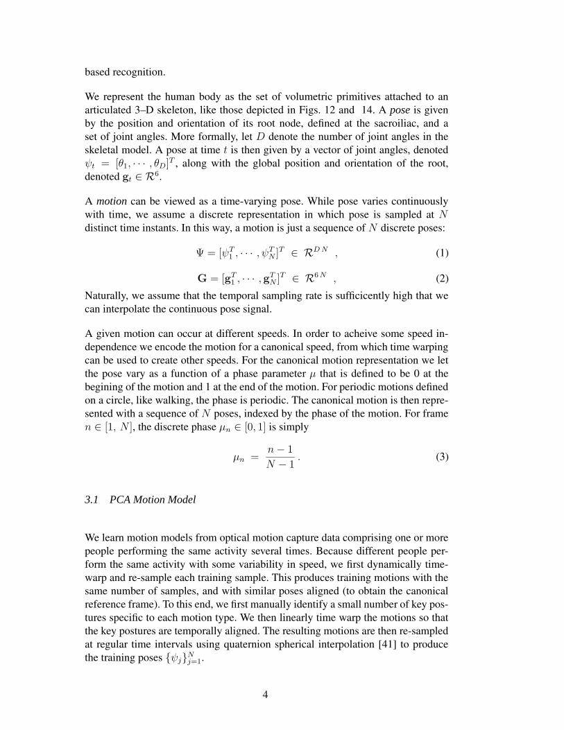
We represent the human body as the set of volumetric primitives attached to anarticulated 3–D skeleton, like those depicted in Figs. 12 and 14. A pose is givenby the position and orientation of its root node, defined at the sacroiliac, and aset of joint angles. More formally, let D denote the number of joint angles in theskeletal model. A pose at time t is then given by a vector of joint angles, denotedψt = [θ1, · · · , θD]T , along with the global position and orientation of the root,denoted gt ∈ R6.

A motion can be viewed as a time-varying pose. While pose varies continuouslywith time, we assume a discrete representation in which pose is sampled at Ndistinct time instants. In this way, a motion is just a sequence of N discrete poses:

Ψ = [ψT1 , · · · , ψ

TN ]T ∈ RD N , (1)

G = [gT1 , · · · ,g

TN ]T ∈ R6 N , (2)

Naturally, we assume that the temporal sampling rate is sufficicently high that wecan interpolate the continuous pose signal.

A given motion can occur at different speeds. In order to acheive some speed in-dependence we encode the motion for a canonical speed, from which time warpingcan be used to create other speeds. For the canonical motion representation we letthe pose vary as a function of a phase parameter µ that is defined to be 0 at thebegining of the motion and 1 at the end of the motion. For periodic motions definedon a circle, like walking, the phase is periodic. The canonical motion is then repre-sented with a sequence of N poses, indexed by the phase of the motion. For framen ∈ [1, N ], the discrete phase µn ∈ [0, 1] is simply

µn =n− 1

N − 1. (3)

3.1 PCA Motion Model

We learn motion models from optical motion capture data comprising one or morepeople performing the same activity several times. Because different people per-form the same activity with some variability in speed, we first dynamically time-warp and re-sample each training sample. This produces training motions with thesame number of samples, and with similar poses aligned (to obtain the canonicalreference frame). To this end, we first manually identify a small number of key pos-tures specific to each motion type. We then linearly time warp the motions so thatthe key postures are temporally aligned. The resulting motions are then re-sampledat regular time intervals using quaternion spherical interpolation [41] to producethe training poses {ψj}

Nj=1.

4

Given a training set of M such motions, denoted, {Ψj}Mj=1, we use Principal Com-

ponent Analysis to find a low-dimensional basis with which we can effectivelymodel the motion. In particular, the model approximates motions in the trainingset with a linear combination of the mean motion Θ0 and a set of eigen-motions{Θi}

mi=1 :

Ψ ≈ Θ0 +m∑

i=1

αiΘi . (4)

The scalar coefficients, {αi}, characterize the motion, and m ≤ M controls thefraction of the total variance of the training data that is captured by the subspace,denoted by Q(m):

Q(m) =

∑mi=1 λi

∑Mi=1 λi

, (5)

where λi are the eigenvalues of the data covariance matrix, ordered such that λi ≥λi+1. In what follows we typically choose m so that Q(m) > 0.9.

A pose is then defined as a function of the scalar coefficients, {αi}, and a phasevalue, µ, i.e.

ψ(µ, α1, · · · , αm) ≈ Θ0(µ) +m∑

i=1

αiΘi(µ) . (6)

Note than now Θi(µ) are eigen-poses, and Θ0(µ) is the mean pose for that particularphase.

3.2 Cyclic motions

We first consider models for walking and running. We used a Vicontm optical mo-tion capture system to measure the motions of two men and two women on a tread-mill:

• walking at 9 speeds ranging from 3 to 7 km/h, by increments of 0.5 km/h, for atotal of 144 motions;

• running at 7 speeds ranging from 6 to 12 km/h, by increments of 1.0 km/h, for atotal of 112 motions.

The body model had D = 84 degrees of freedom. While one might also wish toinclude global translational or orientational velocities in the training data, thesewere not available with the treadmill data, so we restricted ourselves to temporalmodels of the joint angles. The start and end of each gait cycle were manuallyidentified. The data were thereby broken into individual cycles, and normalized sothat each gait cycle was represented with N = 33 pose samples. Four cycles ofwalking and running at each speed were used to capture the natural variability ofmotion from one gait cycle to the next for each person.

5

−15 −10 −5 0 5 10 15 20

−8

−6

−4

−2

0

2

4

6

8

1st PCA component

2nd

PC

A c

ompo

nent

(a) (b)

−10 −5 0 5 10 15 20 25−5

0

5

10

1st PCA component

2n

d P

CA

co

mp

on

en

t

Running

Walking

0 5 10 15 20 25 30 35 40 45 500.4

0.5

0.6

0.7

0.8

0.9

1

(c) (d)

Fig. 1. Motion models. First two PCA components for (a) 4 different captures of 4 subjectswalking at speeds varying from 3 to 7km/h, (b) the same subjects at speeds ranging from6 to 12km/h, (c) the multi-activity database composed of the walking and running motionstogether. The data corresponding to different subjects is shown in different styles. Thesolid lines separating clusters have been drawn manually for visualization purposes. (d)Percentage of the database that can be generated with a given number of eigenvectors for thewalking (dashed red), running(solid green) and the multi-activity databases(dotted blue).

In what follows we learn a motion model for walking and one for running, as wellas multi-activity model for the combined walking and running data. In Fig. 1(d) wedisplay Q(m) in (5) as a function of the number of eigen-motions for the walking,running and the combined datasets. We find that in all three cases m = 5 eigen-motions out of a possible 144 for walking, 112 for running and 256 for the multi-activity data, capture more than 90% of the total variance. In the experiments belowwe show that these motion models are sufficient to generalize to styles that werenot captured in the training data, while eliminating the noise present in the lesssignificant principal directions.

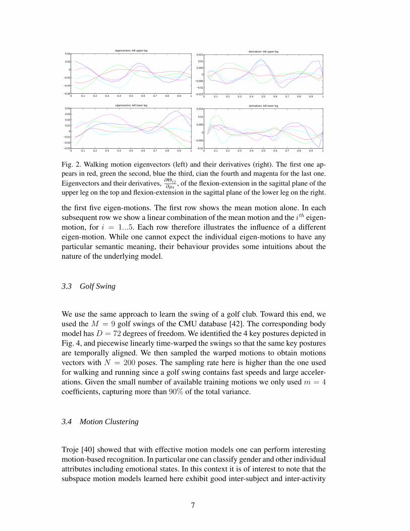
The first five walking eigen-motions, Θi, for the upper and lower leg rotations inthe sagittal plane are depicted by Fig. 2 as a function of the gait phase µt. Onecan see that they are smooth and therefore easily interpolated and differentiatednumerically by finite differences. Fig. 3 illustrates the individual contributions of

6

0 0.1 0.2 0.3 0.4 0.5 0.6 0.7 0.8 0.9 1−0.06

−0.04

−0.02

0

0.02

0.04eigenvectors: left upper leg

0 0.1 0.2 0.3 0.4 0.5 0.6 0.7 0.8 0.9 1−0.03

−0.02

−0.01

0

0.01

0.02

0.03

0.04eigenvectors: left lower leg

0 0.1 0.2 0.3 0.4 0.5 0.6 0.7 0.8 0.9 1−0.015

−0.01

−0.005

0

0.005

0.01

0.015derivatives: left upper leg

0 0.1 0.2 0.3 0.4 0.5 0.6 0.7 0.8 0.9 1−0.01

−0.005

0

0.005

0.01

0.015derivatives: left lower leg

Fig. 2. Walking motion eigenvectors (left) and their derivatives (right). The first one ap-pears in red, green the second, blue the third, cian the fourth and magenta for the last one.Eigenvectors and their derivatives, ∂Θij

∂µt, of the flexion-extension in the sagittal plane of the

upper leg on the top and flexion-extension in the sagittal plane of the lower leg on the right.

the first five eigen-motions. The first row shows the mean motion alone. In eachsubsequent row we show a linear combination of the mean motion and the ith eigen-motion, for i = 1...5. Each row therefore illustrates the influence of a differenteigen-motion. While one cannot expect the individual eigen-motions to have anyparticular semantic meaning, their behaviour provides some intuitions about thenature of the underlying model.

3.3 Golf Swing

We use the same approach to learn the swing of a golf club. Toward this end, weused the M = 9 golf swings of the CMU database [42]. The corresponding bodymodel hasD = 72 degrees of freedom. We identified the 4 key postures depicted inFig. 4, and piecewise linearly time-warped the swings so that the same key posturesare temporally aligned. We then sampled the warped motions to obtain motionsvectors with N = 200 poses. The sampling rate here is higher than the one usedfor walking and running since a golf swing contains fast speeds and large acceler-ations. Given the small number of available training motions we only used m = 4coefficients, capturing more than 90% of the total variance.

3.4 Motion Clustering

Troje [40] showed that with effective motion models one can perform interestingmotion-based recognition. In particular one can classify gender and other individualattributes including emotional states. In this context it is of interest to note that thesubspace motion models learned here exhibit good inter-subject and inter-activity

7

Fig. 3. The top row shows equispaced poses of the mean walk. The next 5 rows illustratethe influence of the first 5 egien-motions. The second row shows a linear combination ofthe mean walk and the first eigen-motion, Θ0 + 0.7Θ1. Similarly, the third row depictsΘ0 + 0.7Θ2 to show the influence of the second eigen-motion, and so on for the remaining3 rows.

Fig. 4. Key postures for the golf swing motion capture database that are used to align thetraining data: Beginning of upswing, end of upswing, ball hit, and end of downswing. Thebody model is represented as volumetric primitives attached to an articulated skeleton.

8

−3 −2 −1 0 1 2 3−2

−1.5

−1

−0.5

0

0.5

1

1.5

2

2.5

3

1

2

−3 −2.5 −2 −1.5 −1 −0.5 0 0.5 1 1.5 2−3

−2

−1

0

1

2

3

3

4

(a) (b)

Fig. 5. Poor clustering in a pose subspace. The solid lines that delimited clusters havebeen manually done for visualization purposes. (a) Projection of training poses onto thefirst two eigen-directions of the pose subspace. (b) Projection of training poses onto thethird and fourth eigen-directions of the pose subspace. While in the motion motion there isstrong inter-subject separation, with the pose model in this figure, there is no inter-subjectseparation.

separation, suggesting that these models may be useful for recognition. For exam-ple, Fig. 1a shows the walking training motions, at all speeds, projected onto thefirst two eigen-motions of the walking model. Similarly, Fig. 1b shows the runningmotions, at all speeds, projected onto the first two eigen-motions of the runningmodel. The closed curves in these figures were drawn manually to help illustratethe large inter-subject separation. One can see that the intra-subject variation inboth models is much smaller than the inter-subject variation.

The motion model learned from the combination of walking and running trainingdata shows large inter-activity separation. Fig. 1c shows the projection of the train-ing data onto the first two eigen-motions of the combined walking and runningmodel. One can see that the two activities are easily separated in this subspace. Thewalking components appear on the left of the plot and form a relatively dense set.By contrast, the running components are sparser because inter-subject variation islarger, indicating that more training examples are required for a satisfactory model.

While the motion models exhibit this inter-subject and inter-activity variation, wewould not expect pure pose models to exhibit similar structure. For example todemonstrate this we also learned a pose model by applying PCA on individualposes in the same dataset. Fig. 5 shows poses from the walking data projectedonto the first four eigen-directions of the subspace model learned from poses inthe walking motions. It is clear that there is no inter-subject separation in the posemodel.

9

−8 −6 −4 −2 0 2 4 6 8 10−8

−6

−4

−2

0

2

4

6

1st PCA component

2nd

PC

A c

ompo

nent

Sample

Origin

−15 −10 −5 0 5 10 15 20

−8

−6

−4

−2

0

2

4

6

8

1st PCA component

2nd

PC

A c

ompo

nent

Sample

Origin������

−10 −5 0 5 10 15−6

−4

−2

0

2

4

6

8

10

12

1st PCA component

2nd

PC

A c

ompo

nent Sample

Origin

������

(a) (b) (c)

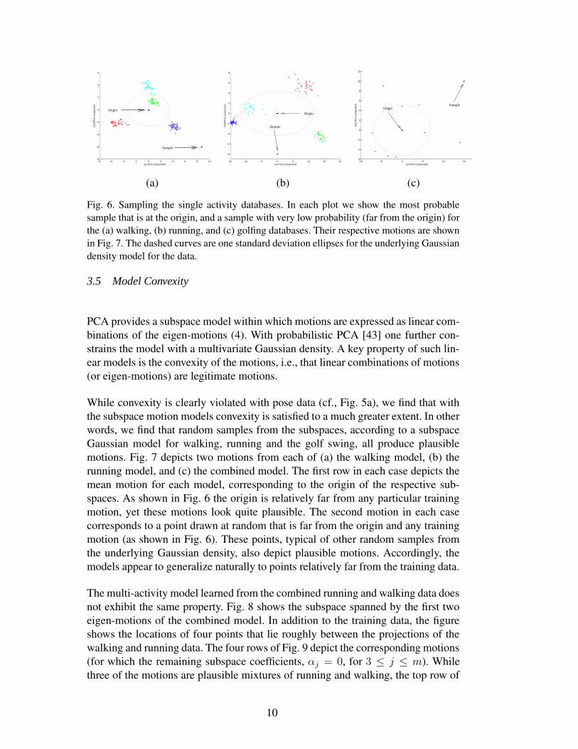
Fig. 6. Sampling the single activity databases. In each plot we show the most probablesample that is at the origin, and a sample with very low probability (far from the origin) forthe (a) walking, (b) running, and (c) golfing databases. Their respective motions are shownin Fig. 7. The dashed curves are one standard deviation ellipses for the underlying Gaussiandensity model for the data.

3.5 Model Convexity

PCA provides a subspace model within which motions are expressed as linear com-binations of the eigen-motions (4). With probabilistic PCA [43] one further con-strains the model with a multivariate Gaussian density. A key property of such lin-ear models is the convexity of the motions, i.e., that linear combinations of motions(or eigen-motions) are legitimate motions.

While convexity is clearly violated with pose data (cf., Fig. 5a), we find that withthe subspace motion models convexity is satisfied to a much greater extent. In otherwords, we find that random samples from the subspaces, according to a subspaceGaussian model for walking, running and the golf swing, all produce plausiblemotions. Fig. 7 depicts two motions from each of (a) the walking model, (b) therunning model, and (c) the combined model. The first row in each case depicts themean motion for each model, corresponding to the origin of the respective sub-spaces. As shown in Fig. 6 the origin is relatively far from any particular trainingmotion, yet these motions look quite plausible. The second motion in each casecorresponds to a point drawn at random that is far from the origin and any trainingmotion (as shown in Fig. 6). These points, typical of other random samples fromthe underlying Gaussian density, also depict plausible motions. Accordingly, themodels appear to generalize naturally to points relatively far from the training data.

The multi-activity model learned from the combined running and walking data doesnot exhibit the same property. Fig. 8 shows the subspace spanned by the first twoeigen-motions of the combined model. In addition to the training data, the figureshows the locations of four points that lie roughly between the projections of thewalking and running data. The four rows of Fig. 9 depict the corresponding motions(for which the remaining subspace coefficients, αj = 0, for 3 ≤ j ≤ m). Whilethree of the motions are plausible mixtures of running and walking, the top row of

10

Fig. 9 clearly shows an implausible motion. Here we find that points close to thetraining data generate plausible motions, but far from the training data the motionsbecome less plausible.

Nevertheless there are regions of the subspace between walking and running datapoints that do correspond to plausible models. These regions facilitate transitionsbetween walking and running that are essential if we wish to be able to track sub-jects through such transitions, as will be shown in section 6.

4 Tracking Framework

In this section we show how the motion models of Section 3 can be used for 3D peo-ple tracking. Our goal is to show that with activity-specific motion models one canoften formulate and solve the tracking problem straightforwardly with deterministicoptimisation. Here, tracking is expressed as a nonlinear least-squares optimization,and then solved using Levenberg-Marquardt [44].

The tracking is performed with a sliding temporal window. At each time instant twe find the optimal target parameters for f frames within a temporal window fromtime t to time t+ f − 1. Within this window, the relevant target parameters includethe subspace coefficients, {αi}

mi=1, the global position and orientation of the body at

each frame {gj} and the phases of the motion at each frame {µj}, for t ≤ j < t+f :

St = [α1, . . . , αm, µt, . . . , µt+f−1,gt, . . . ,gt+f−1] . (7)

While the global pose and phase of the motion vary throughout the temporal win-dow, the unknown subspace coefficents are assumed to be constant over the win-dow.

After minimizing an objective function over the unknown parameters St, we extractthe pose estimate at time t that is given by the estimated subspace coefficients{αi}, along with the global parameters and phase at time t, i.e., gt and µt. Becausethe temporal estimation windows overlap from one time instant to the next, theestimated target parameters tend to vary smoothly over time. In particular, with sucha sliding window the estimate of the pose at time t is effectively influenced by bothpast and future data. It is influenced by past data because we assume smoothnessbetween parameters at time t and estimates already found at previous time instantst− 1 and t− 2. It is influenced by future data as data constraints on the motion areobtained from image frames at times t+ 1 through t+ f − 1.

11

(a)

(b)

(c)

Fig. 7. Sampling the first five components of each single activity database produce phys-ically possible motions. The odd rows show the highest probability sample that for eachsingle-motion database, which is the at the origin αi = 0, ∀i. The even rows show somelow probability samples very far from the training motions to demonstrate that even thosesamples produce realistic motions. The coefficients for these motion are shown in Fig. 6(a,b,c) respectively. First two rows (a): Walking, Middle rows (b): Running, Last tworows (c): Golf swing samples.

12

−15 −10 −5 0 5 10 15 20 25−10

−8

−6

−4

−2

0

2

4

6

8

10

1st PCA component

2nd

PC

A c

ompo

nent

(4)

(2)

(3)

(1)

Fig. 8. Sampling the multi-activity subspace. The 4 samples that generate the motions ofFig. 9 are depicted.

Fig. 9. Sampling the first two components of a multi-activity database compose of walkingand running motions can produce physically impossible motions. The coefficients of themotions depicted in this figure are shown in Fig. 8. Top row: Physically impossible mo-tion. The input motion space compose of walking and running is not convex. Middle row:Physically possible motion close to a walking. Bottom row: Motion close to a running. Asthe convexity of the input space is assumed when doing PCA, and it may not be the case,the resulting motion as a combination of principal directions can be physically impossible.

13

4.1 Objective Function

We use the image data to constrain the target parameters with a collection of nobs

constraint equations of the form

O(xi,S) = εi , 1 ≤ i ≤ nobs , (8)

where the xi are 2D image features, O is a differentiable function whose valueis zero for the correct value of S and noise-free data, and εi denotes the residualerror in the ith constraint. Our objective is to minimize the sum of the squaredconstraint errors. Because some measurements may be noisier than others, and ourobservations may come from different image properties that might not be commen-surate with one another, we weight each constraint of type type with a constant,wtype. In effect, this is equivalent to a model in which the constraint residuals areIID Gaussian with isotropic covariance, and the weights are just inverse variances.In practice, the values of the different wtype are chosen heuristically based on theexpected errors for each type of observation.

Finally, since image data are often noisy, and sometimes underconstrain the targetparameters, we further assume regularization terms that encourage smoothness inthe global model. We also assume that the phase of the motion varies smoothly. Theresulting total energy to be minimized at time t, Ft, can therefore be expressed as

Ft = Fo,t + Fg,t + Fµ,t + Fα,t (9)

with

Fo,t =nobs∑

i=1

wtypei

∥

∥

∥Otypei(xi,S)∥

∥

∥

2

, Fg,t = wG

t+f−1∑

j=t

‖gj − 2gj−1+ gj−2‖2 ,

Fµ,t =wµ

t+f−1∑

j=t

(µj − 2µj−1+ µj−2)2 , Fα,t = wα

m∑

i=1

(αi − αi)2 , (10)

where Otype is the function that corresponds to a particular observation type, wG,wµ and wα are scalar weights, and αi denote the subspace coefficients estimatedin the previous window of f frames at time t − 1. The value of f is chosen to besufficiently large to produce smooth results; in practice we use f = 3. Finally, in(10), the variables gt−1, gt−2, µt−1 and µt−2 are taken to be the values estimatedfrom previous two time instants, and are therefore fixed during estimation at timet.

Minimizing Ft using the Levenberg-Marquardt algorithm [44] involves computingits Jacobian with respect to the elements of the state vector S. Since the O func-tions of Eq. 10 are differentiable with respect to the elements of S, computing the

14

derivatives with respect to the gt is straightforward. Those with respect to the αi

and µt can be written as

∂Ft

∂αi

=t+f−1∑

k=t

D∑

j=1

∂Fo,t

∂θkj

·∂θk

j

∂αi

+∂Fα,t

∂αi

, (11)

∂Ft

∂µk

=D∑

j=1

∂Fo,t

∂θkj

·∂θk

j

∂µk

+∂Fµ,t

∂µk

, (12)

where the θkj represents the vector of individual joint angles at phase µk, defined

as the j’th component of ψ(µk, α1, · · · , αm) in Eq. 6. The derivatives of Ft withrespect to theD individual joints angles ∂Fo,t

∂θkj

can be easily computed [45]. Because

the θkj are linear combinations of the Θk

ij eigen-poses, ∂θkj

∂αireduces to Θk

ij , the jthcoordinate of Θk

i . Similarly, we can write

∂θkj

∂µk

=m∑

i=1

αi

∂Θkij

∂µk

, (13)

where the ∂Θkij

∂µtcan be evaluated using finite differences and stored when building

the motion models, as depicted in Fig. 2.

Recall that for cyclic motions such as walking and running, the phase is periodicand hence the second order prediction µj−1 − µj−2 should be taken mod 1 inEq. 9. This allows the cyclic tracking sequences to be arbitrarily long, not just asingle cycle. Of course, one can also track sequences that comprise fractional partsof either cyclic or acyclic motion model.

The weights w in Eq. (10) were set manually, but their exact values were not foundto be particularly critical. In some experiments the measurements provided suffi-cient strong constraints that the smoothness energy terms in Eq. (10) played a veryminor role; in such cases the values of wG, wµ and wα could be set much smallerthan the weights on the measurement errors in Fo,t. Nonetheless, for each set ofexperiments below (i.e, those using the same types of measurements), the weightswere fixed across all input sequences.

4.2 Computational Requirements

The fact that one can track effectively with straight-forward optimization meansthat our prior motion models greatly constrain the inference problem. That is, theresulting posterior distributions are not so complex (e.g., multimodal) that one mustuse computationally demanding inference methos such as sequential Monta Carloor particle filtering.

15

Monte Carlo approaches, like that in [8], rely on randomly generating particlesand evaluating their fitness. Because the cost of creating particles is negligible, themain cost of each iteration comes from evaluating a log likelihood, such as Ft in(9), for each particle. In a typical particle filter, like the Condensation algorithm[7], the number of particles needed to effectively approximate the posterior on aD-dimensional state space grows exponentially with D [5,46]. With dimensionalityreduction, like that obtained with the subspace motion model, the state dimensionis greatly reduced. Nevertheless, the number of particles required can still be pro-hibitive [8].

By contrast, the main cost at each iteration of our deterministic optimization schemecomes from evaluating Ft and its Jacobian. In our implementation, this cost isroughly proportional to 1 + log(D) times the cost of computing Ft alone, whereD is the number of joint angles of (12). The reason this factor grows slowly withD is that the partial derivatives, ∂Ft

∂θj, which require most of the computation, are

computed analytically and involve many intermediate results than can be cachedand reused. As a result, with R iterations per frame, the total time required by ouralgorithm is roughly proportional R(1 + log(D)) times the cost of evaluating Ft.Since we use a small number of iterations, less than 15 for all experiments in thispaper, the total cost of our approach remains much smaller than typical probabilis-tic methods. The different experiments run in this paper took less than a minute perframe, with a non-optimized implementation.

5 Monocular Tracking

We first demonstrate our approach in the context of monocular tracking [47]. Sincewe wish to operate outdoors in an uncontrolled environment, tracking people wear-ing normal clothes, it is difficult to rely solely on any one image cue. Here wetherefore take advantage of several sources of information.

5.1 Projection Constraints

To constrain the location of several key joints, we track their approximate imageprojections across the sequence. These 2D joint locations were estimated with a2D image-based tracker. Figure 10 shows the 2D tracking locations for two testsequences; we track 9 points for walking sequences, and 6 for the golf swing.

For joint j, we therefore obtain approximate 2–D positions xj in each frame. Fromthe target parameters S we know the 3–D position of the corresponding joint. Wethen take the corresponding constraint function, Ojoint(xj,S), to be the 2–D Eu-clidean distance between the joint’s projection into the image plane and the mea-

16

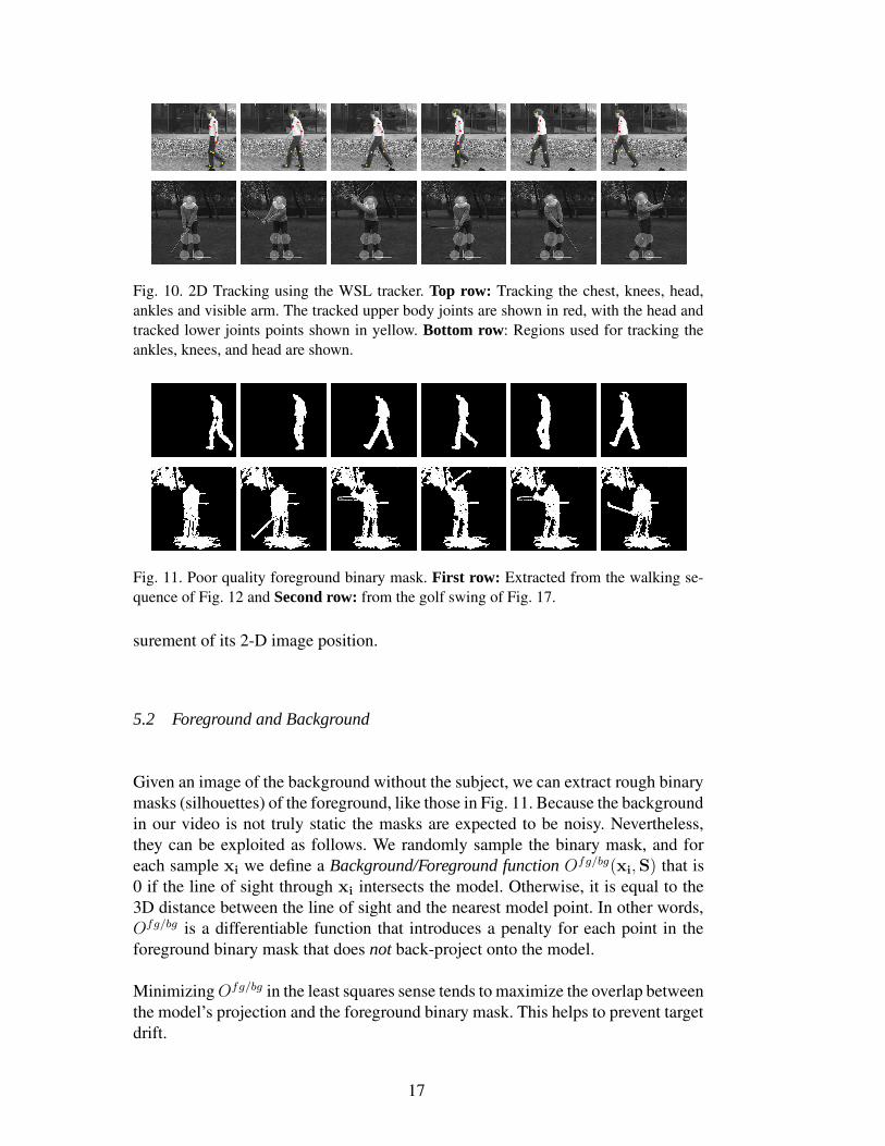
Fig. 10. 2D Tracking using the WSL tracker. Top row: Tracking the chest, knees, head,ankles and visible arm. The tracked upper body joints are shown in red, with the head andtracked lower joints points shown in yellow. Bottom row: Regions used for tracking theankles, knees, and head are shown.

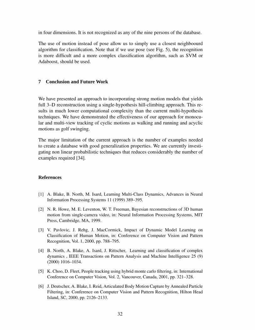
Fig. 11. Poor quality foreground binary mask. First row: Extracted from the walking se-quence of Fig. 12 and Second row: from the golf swing of Fig. 17.

surement of its 2-D image position.

5.2 Foreground and Background

Given an image of the background without the subject, we can extract rough binarymasks (silhouettes) of the foreground, like those in Fig. 11. Because the backgroundin our video is not truly static the masks are expected to be noisy. Nevertheless,they can be exploited as follows. We randomly sample the binary mask, and foreach sample xi we define a Background/Foreground function Ofg/bg(xi,S) that is0 if the line of sight through xi intersects the model. Otherwise, it is equal to the3D distance between the line of sight and the nearest model point. In other words,Ofg/bg is a differentiable function that introduces a penalty for each point in theforeground binary mask that does not back-project onto the model.

MinimizingOfg/bg in the least squares sense tends to maximize the overlap betweenthe model’s projection and the foreground binary mask. This helps to prevent targetdrift.

17

5.3 Point Correspondences (Optical Flow)

We use 2–D point correspondences in pairs of consecutive images as an additionalsource of information: We project the 3–D model into the first image of the pair.We then sample image points to which the model projects and use a normalizedcross-correlation algorithm to compute displacements of these points from thatframe to the next. This provides us with measurement pairs of corresponding pointsin two consecutive frames, pi = (x1

i ,x2i ). The correspondence penalty function,

Ocorr(pi,S) is given as follows: We back-project x1i to the 3–D model surface and

reproject it to the second image. We then take Ocorr(pi,S) to be the Euclideandistance in the image plane between this reprojection and corresponding x2

i .

5.4 Experimental Results

We test our tracker on real and synthetic data. In each case the use of prior mo-tion models is crucial; without the motion models the tracker diverge within a fewframes in every experiment.

5.4.1 Real data

The results shown here were obtained from uncalibrated images. The motions wereperformed by subjects of unknown sizes wearing ordinary clothes that are not par-ticularly textured. To perform our computation, we used rough guesses for the sub-ject sizes and for the intrinsic and extrinsic camera parameters. For each test se-quence we manually initialize the position and orientation of the root node of thebody in the first frame so that it projects approximately to the right place.

We also manually specify the 2D locations of the joints to be tracked by WSL [48].WSL is a robust, motion-based 2D tracker that maintains an online adaptive appear-ance model. The model adapts to slowly changing image appearance with a naturalmeasure of the temporal stability of the underlying image structure. By identifyingstable properties of appearance the tracker can weight them more heavily for mo-tion estimation, while less stable properties can be proportionately down-weighted.This gives it robustness to partial occlusions. In the first frame we specified 9 pointsthat we wish to track, namely, the ankles, knees, chest, head, left shoulder, elbowand hand.

This entire process requires only a few mouse clicks and could easily be improvedby using automated posture detection techniques (e.g., [20,26,21,22,24]). Simplemethods were used to detect the key postures defined in Section 3 for each se-quence. Using spline interpolation, we assign an initial value for µt for all theframes in the sequence, as depicted in Figs. 13b and 16b. Finally, the motion is ini-

18

Fig. 12. Monocular Tracking of a 43 frames walking motion. First two rows: The skeletonof the recovered 3D model is projected onto the images. Bottom two rows: Volumetricprimitives of the recovered 3D model projected into a similar view.

tially taken to be the mean motion Θ0, i.e., the subspace coefficients αi are initiallyset to zero. Given these initial conditions we minimize Ft in (9) using Levenberg-Marquardt.

5.4.1.1 Walking Fig. 12 shows a well-known walking sequence [8,49,50]. Toperform the 2D tracking we used a version of the WSL tracker [48]. To initialize thephase parameter, µt, we used a simple background subtraction method to computeforeground masks (e.g., see Fig. 11). Times at which the mask width was minimalwere taken to be the times at which the legs were together (i.e., µt = 0.25 orµt = 0.75). Spline interpolation was then used to approximate µt at all other framesin the sequence (see Fig. 13b). More sophisticated detectors [20–22,24] would benecessary in more challenging situations, but were not needed here.

The optimal motion found is shown in Figure 12. There we show the estimated 3Dmodel projected onto several frames of the sequence. We also show the rendered3D volumetric model alone. The tracker was successful, producing a 3D motionthat is plausible and well synchronized with the video. The right (occluded) armwas not tracked by the WSL tracker, and hence was only weakly constrained by theobjective function. Note that even though it is not well reconstructed by the model(does not fit the image data), it has a plausible rotation.

5.4.1.2 Golf Swing As discussed in Section 3.3, the golf swings used to trainthe model were full swings from the CMU database. They were performed by nei-

19

0 5 10 15 20 25 30 35 40 45130

135

140

145

150

155Horizontal mask size

frames

x−pi

xel

0 5 10 15 20 25 30 35 40 451.2

1.4

1.6

1.8

2

2.2

2.4

2.6

2.8

frames

virt

ual t

ime

Spline interpolation virtual time

(a) (b)

Fig. 13. Automatic Initialization of the virtual time parameter µt for the walking sequenceof Fig. 12. (a) Width of the detected silhouette. (b) Spline interpolation for the detectedkey-postures.

Fig. 14. Monocular Tracking a full swing in a 45 frame sequence. First two rows: Theskeleton of the recovered 3–D model is projected into a representative subset of images.Middle two rows: Volumetric primitives of the recovered 3–D model projected into thesame views. Bottom two rows: Volumetric primitives of the 3–D model as seen fromabove.

20

220 240 260 280 300 320 340 360 380 400 420150

200

250

300

350

400Hands detection

pixel x

pixe

l y

200 250 300 350 400 450160

180

200

220

240

260

280

300

320

340

360Hands detection

pixel x

pixe

l y

220 240 260 280 300 320 340 360 380 400 420180

200

220

240

260

280

300Hands detection

pixel x

pixe

l y

(a) (b) (c)

Fig. 15. Detected hand trajectories for the full swing in Fig. 14 and the approach swingin Fig. 18. The left and right hand positions (pixel units) are represented in black and redrespectively.

ther of the golfers shown in Figs. 14, 17 and 18. With the WSL tracker we trackedfive points on the body, namely, the knees, ankles and head (see Fig. 10). Becausethe hand tends to rotate during the motion, to track the wrists we have found itmore effective to use a club tracking algorithm [51] that takes advantage of theinformation provided by the whole shaft. Its output is depicted by the first row ofFig. 15, and the corresponding recovered hand trajectories by the second row. Thistracker does not require any manual initialization. It is also robust to mis-detectionsand false alarms and has been validated on many sequences. Hypotheses on the po-sition are first generated by detecting pairs of close parallel line segments in theframes, and then robustly fitting a 2D motion model over several frames simulta-neously. From the recovered club motion, we can infer the 2D hand trajectories ofthe bottom row of Fig. 15.

For each sequence, we first run the golf club tracker [51]. As shown in Fig. 16a, foreach sequence, the detected club positions let us initialize the phase parameters bytelling us in which four frames the key postures of Fig. 4 can be observed. With thetimes of the key postures, spline interpolation is then used to assign a phase to allother frames in the sequence (see Fig. 16b). As not everybody performs the motionat the same speed, these phases are only initial guesses, which are refined duringthe actual optimization. Thus the temporal alignment does not need to be precise,but it gives a rough initialization for each frame.

Figures 14 and 17 show the projections of the recovered 3D skeleton in a repre-sentative subset of images of two full swings performed by subjects whose motion

21

80 90 100 110 120 130 140 150 160 170 1800

0.1

0.2

0.3

0.4

0.5

0.6

0.7

0.8

0.9

1

Nor

mal

ized

tim

e

Frame number

(a) (b)

Fig. 16. Assigning normalized times to the frames of Fig. 14. (a) We use the automaticallydetected club positions to identify the key postures of Fig. 4. (b) The corresponding nor-malized times are denoted by red dots. Spline interpolation is then used to initialize the µt

parameter for all other frames in the sequence.

Fig. 17. Monocular tracking a 68 frame swing sequence. The skeleton of the recovered 3–Dmodel is projected onto the images.

was not used in the motion database. Note the accuracy of the results. Figure 18depicts a short swing that is performed by a different person. Note that this motionis quite different both from the full swing motion of Fig. 14 and from the swingused to train the system. The club does not go as high and, as shown in Fig. 15, thehands travel a much shorter distance. As shown by the projection of the 3D skele-ton, the system has enough flexibility to generalize to this motion. Note, however,that the right leg bends too much at the end of the swing, which is caused by thesmall number of training motions and the fact that every training swing exhibitedthe same anomoly. A natural way to avoid this problem in the future would be touse a larger training set with a greater variety of motions.

Finally, Fig. 19 helps to show that the model has sufficient flexibility to do thewrong thing given insufficient image data. That is, even though we use an activity-specific motion model, the problem is not so constrained that we are guaranteed toget valid postures or motions without using the image information correctly.

22

Fig. 18. Monocular Tracking an approach swing during which the club goes much lesshigh than in a driving swing. The skeleton of the recovered 3–D model is projected ontothe images.

(a) (b) (c) (d) (e) (f)

Fig. 19. Tracking using only joint constraints vs using the complete objective function. (a)Original image. (b) 2–D appearance based tracking result. (c) 2–D projection of the trackingresults using only joint constraints. The problem is under-constrained and a multiple set ofsolutions are possible. (d) 3–D tracking results using only joint constraints. (e) and (f) Theset of solutions is reduced using correspondences.

5.4.2 Synthetic data

We projected 3D motion capture data using a virtual camera to produce 2D jointpositions that we then use an input to our tracker. The virtual camera is such thatthe projections fall within a 640x480 virtual image, with the root projecting at thecenter of the image. We initialized the phase of the motion µt to a linear function,0 at the beginning and 1 at the end of the sequence. The style of the motion wasinitialized to be the mean motion. Both µt and the {αi} were refined during thetracking.

We used temporal windows of sizes 3 and 5, with very similar results, as shown inFig. 20. We also tested the influence of the number of 2D joint positions given asinput to the tracker, by using the whole set of joints, or the same subset of jointsused to track the sequence of Fig. 12, namely, the ankles, knees, chest, head, shoul-der, elbow and hand. Both cases result in very similar accuracy, as depicted in Fig.20. The errors, as expected, are bigger when tracking testing data than training data.Note that the tracker is very accurate, the 3D errors are 0.7 cm per joint in mean forthe training sequences and 1.5 cm in mean for the testing sequences.

It is also of interest to test the sensitivity of the tracker to the relative magnitudesof the smoothness and observation weights in Eq. (10). Fig. 21 shows the results oftracking synthetic training and testing sequences with different values of wtype/ws,

23

Training Test

2D proj. 3D loc. Euler 2D proj. 3D loc. Euler

All, f = 3 0.960 7.271 0.031 1.849 15.079 0.086

Subset, f = 3 1.024 7.575 0.0322 1.979 15.062 0.0839

All, f = 5 1.093 7.246 0.0272 2.041 15.823 0.087

Subset, f = 5 1.153 7.721 0.0293 2.182 15.791 0.0847

1 20

0.5

1

1.5

2

2.5ik

1 20

2

4

6

8

10

12

14

16trajectories

1 20

0.01

0.02

0.03

0.04

0.05

0.06

0.07

0.08

0.09euler

2D projection 3D location Euler angles

Fig. 20. Tracking mean errors as a function of the window size and the number of 2Dconstraints. Three types of errors (2D projection (pixels), 3D location (mm), Euler angles(radians) are depicted. Each plot is split in two groups, the left one represents errors whentracking training data and the right one test data. For each group 4 error bars of 2 differentcolors are depicted, each color represents a different window size (3 on red, and 5 on green).For each color two bars show the errors first for the complete set of joints and then for thesubset of joints, with similar results. Note that the estimated 3D joint location errors arevery small, 0.7 cm in mean for the training data sequences, and 1.5 cm for the testing ones.

ranging from 0.1 to 10, with ws = wg = wµ = wα. All experiments yielded similarresults, indicating that the tracker is not particularly sensitive to these parameters.

5.4.3 Failure Modes

We have demonstrated that the tracking works well for different cyclic (walking)and a-cyclic motions (golfing). The tracked motions are different from the onesused for training, but remain relatively close. In this section we use a caricaturedwalking sequence to test when the generalization capabilities of our motion modelsfail. The caricatured walking is very different from the motions used for training,and the PCA-based motion models do not generalize to this motion well. The stylecoefficients recovered by the tracker are very far from the training ones (at least6 standard deviations), resulting in impossible poses as depicted by Fig. 22, whenusing a 3 or 5 frame temporal window.

When using PCA-based motion models, one should track motions that remain rel-atively close to the training data, since the only motions that the tracker is capableof producing are those in the subspace. In case other motions are wanted to be

24

Training Test

2D proj. 3D loc. Euler 2D proj. 3D loc. Euler

wtype/ws = 0.1 1.262 7.979 0.0291 2.104 15.621 0.0865

wtype/ws = 1 1.632 9.895 0.0347 2.384 14.692 0.0715

wtype/ws = 10 1.808 12.263 0.0339 2.812 16.934 0.0728

1 20

0.5

1

1.5

2

2.5

3ik

1 20

2

4

6

8

10

12

14

16

18trajectories

1 20

0.01

0.02

0.03

0.04

0.05

0.06

0.07

0.08

0.09euler

2D projection 3D location Euler angles

Fig. 21. Tracking mean errors as a function of the weights. Tracking results are givenfor experiments with three different types of measurement errors (2D projection (pixels),3D location (mm), Euler angles (radians)). Each plot is split in two groups, the left one rep-resents errors when tracking training data and the right one for tracking test data. For eachgroup 3 error bars of different colors are depicted. Each color represents different relativeweights (dark green wtype/ws = 0.1, green wtype/ws = 1, and yellow wtype/ws = 10),with ws = wg = wµ = wα. Note that tracker is not very sensitive to the specific value ofthe weights.

Fig. 22. Tracking 40 frames of an exaggerated gait. First two rows: 3 frame window. Lasttwo rows: 5 frame window. The tracker results in impossible positions.

tracked, one should include examples of such motions when learning the models,or apply other techniques such as Gaussian Processes (GP) [34] that have bettergeneralization properties.

25

6 Multi-view Tracking

When several synchronized video streams are available, we use a correlation-basedstereo algorithm [52] to extract a cloud of 3–D points at each frame, to which wefit the motion model.

6.1 Objective Function

Recall from Section 3 that we represent the human body as a set of volumetricprimitives attached to an articulated 3–D skeleton. For multi-view tracking we treatthem as implicit surfaces as this provides a differentiable objective function whichcan be fit to the 3D stereo data while ignoring measurement outliers. Following[45] the body is divided into several body parts; each body part b includes nb ellip-soidal primitives attached to the skeleton. Associated with each primitive is a fieldfunction fi, of the form

fi(x,S) = bi exp(−aidi(x,S)) , (14)

where x is a 3–D point, ai, bi are constant values, di is the algebraic distance to thecenter of the primitive, and S, is the state vector in (7). The complete field functionfor body part b is taken to be

f b(x,S) =nb∑

i=1

fi(x,S) , (15)

and the skin is defined by the level set

SK(x,S) =B⋃

b=1

{x ∈ R3|f b(x,S) = C} (16)

where C is a constant, and B is the total number of body parts. A 3D point x is saidattached to body part b if

b = arg min1≤i≤B

|f i(x,S) − C| (17)

For each 3D stereo point, xi, we write

Ostereo(xi,S) = f b(xi,S) − C . (18)

Fitting the model to stereo-data then amounts to minimizing (9), the first term ofwhich becomes

t+f−1∑

j=t

B∑

b=1

∑

xi∈b

(f b(xi,j,S) − C)2 , (19)

26

Fig. 23. Tracking a running motion. The legs are now correctly positioned in the wholesequence.

where xi,j is a 3D stereo point belonging to frame j. Note that Ostereo is differen-tiable and its derivatives can be computed efficiently [45].

6.2 Experimental Results

We use stereo data acquired using a Digiclopstm operating at a 640×480 resolutionand a 14Hz frame rate. Because the frame rate is slow, the running subject of Fig. 23remains within the capture volume for only 6 frames. The data shown in Fig. 24 arenoisy and have low resolution for two reasons. First, to avoid motion blur, we useda high shutter speed that reduced exposure. Second, because the camera was fixedand the subject had to remain within the capture volume, she projected onto a smallregion of the image during the sequences. Of course, the quality of this stereo datacould have been improved by using more sophisticated equipment. Nevertheless,our results show that the tracker is robust enough to exploit data acquired withcheap sensors.

Initially, the motion subspace coefficients are set to zero, as above. We manuallyinitialized the phase of the motion µt in the first and last frame of the sequence.These points were then interpolated to produce an initial phase estimate in everyframe. The initial guess does not have to be precise because the tracking does notwork directly with the images but with the 3D data.

Fig. 25 shows results on walking sequences performed by two subjects whose mo-tion capture data were also used as training data for the motion models. One can seefrom the figures that the legs are correctly positioned. The errors in the upper-bodyare caused by the large amount of noise in the stereo data.

Figure 26 depicts results from a walking sequence with a subject whose motion wasnot included in the training data. In this case he was also wearing four gyroscopeson his legs, one for each sagittal rotation of the hip and knee joints. The angular

27

Fig. 24. Input stereo data for the running sequence of Fig. 23. Side views of the 3–D pointscomputed by the Digiclops tm system. Note that they are very noisy and lack depth becauseof the low quality of the video sequence.

Fig. 25. Using low resolution stereo data to track the two women whose motions were notused to learn the motion model. The recovered skeleton poses are overlaid in white.

speeds they measured were used solely for comparison purposes. Their output wasintegrated to yield the absolute angles shown as dotted curve in Fig. 27. We overlayon these plots the values recovered by our tracker, showing that they are close, eventhough the left leg is severely occluded. Given the position of the visible leg, thePCA motion model constrains the occluded one to be in a plausible position closeto the real one.

Figure 23 shows results for the running sequence of Fig. 24 using the running mo-tion model. The pose of the legs is correctly recovered. The upper body trackingremains relatively imprecise because average errors in the stereo data are larger

28

Fig. 26. Tracking a walking motion from a subject whose motion was not recorded in thedatabase. The legs are correctly positioned.

0 2 4 6 8 10 12 14 16−0.2

0

0.2

0.4

0.6

0.8

1

0 2 4 6 8 10 12 14 16

−1.2

−1

−0.8

−0.6

−0.4

−0.2

0

0 2 4 6 8 10 12 14 16

−0.6

−0.4

−0.2

0

0.2

0.4

0.6

0 2 4 6 8 10 12 14 16

−0.6

−0.4

−0.2

0

0.2

0.4

0.6

Fig. 27. Comparing recovered rotation angles using visual tracking (solid curve), and byintegrating gyroscopic data (smooth curve) for the walk of Fig. 26. Left column: Righthip and knee sagittal rotations. Right Column: Same thing for the left leg. Note that bothcurves are very close in all plots, even though the left leg is severely occluded.

than the distance between the torso and the arms. Improving this would requirethe use of additional information, such as silhouettes. Here we restrict ourselves tostereo data to show that our framework can be used with very different objectivefunctions.

Having a set of subspace coefficients per frame gives the system the freedom toautomatically evolve from one activity to another. To demonstrate this we usedour motion model learned for the combined running and walking data to track atransition from walking to running (see Fig. 28). In the first few frames the subjectis walking, then for a couple of frames she performs the transition and runs for therest of the sequence. The arms are not tracked because we focus on estimating themotion parameters of the lower body only. Here again, the legs are successfullytracked with small errors in foot positioning that are due to the fact that ankleflexion is not part of the motion database.

6.3 Recognition

The motion style is encoded by the subspace coefficients in (4). They measure thedeviation from the average motion along orthogonal directions. Recall that duringtracking, the subspace coefficients are permitted to vary from frame to frame. Forrecognition, we further reconstruct the 3D motion of the person with a single set

29

Fig. 28. Tracking the transition between walking and running. In the first four frames thesubject is running. The transition occurs in the following three frames and the sequenceends with running. The whole sequence is shown.

Fig. 29. Style coefficents, αi, obtained when tracking a training sequence. The trainingdata is shown in cyan. Different colors show different window sizes and number of 2Djoint constraints.

of subspace coefficients for the entire sequence [53]. The reason is that we wantto recover an average motion style during the sequence. Moreover, the estimate ofthe style coefficients is more reliable if we increase the number of poses we useto obtain it If we allow the style parameters to vary from frame to frame the styleestimation is noisier, but the tracker is typically more accurate. This is illustratedin Fig. 29, when tracking with ground truth data and varying the subspace coeffi-cients. Note that although the coefficients are close to the ones of that subject, theirvariance is relatively large.

The tracking algorithm used for recognition is divided into two steps. First, the nor-malized time µt and the global motion gt are optimized frame by frame, assuminga constant style equal to the mean motion Θ0. This provides a good initial estimatefor a second step, where a global optimization is performed. In the global fit, thenormalized time and global motion parameters are allowed to vary in every frame,but only one set subspace coefficients is used to represent the entire motion se-quence. This is equivalent to minimizing (9), where the size of the sliding window

30

(a) (b) (c)

Fig. 30. Recognition of walking people from stereo data: Walking motions from the trainingdata are shown in the first four subspace dimensions. Each person is shown with a distinctcolor and symbol. Small black circles denote the estimated subspace coefficients, αi, ob-tained from video of people whose motions were included in the training set. The smallblack triangles depict subspace coefficients obtained from video of people whose motionswere not included in the training set. (a) First two PCA components of a model learnedfrom 4 subjects. Notice that in the first two dimensions the estimated coefficients for thetest subject are easily confused with those of the training subjects. (b-c) First four compo-nents of a model learned with 9 subjects. In the first four dimensions the motions of thetraining subjects cluster nicely, and the subspace coefficients estimated for a test subject donot lay close to any one cluster of the training subjects.

is f = T + 1.

Figure 30 (a) depicts the first two subspace coefficients, αi, for the database usedfor the tracking. The four subjects of the subspace are well separated in the first twodimensions. The estimated coefficients for each one of the two examples depictedby Fig. 25 are shown as circles and a triangle represents the estimated value for thesubject in Fig. 26 whose motion is not included in the training dataset. For bothwomen, the first two recovered coefficients fall in the center of the cluster formedby their recorded motion vectors. Also note that while the new subject’s motiondoes appear consistent with one of the training subjects in the first two subspacedimensions, they are quite different in the next two dimensions.

Figure 30 (b,c), depicts the first four subspace coefficients, αi, for a model learnedusing nine subjects. The estimated coefficients for each one of the two examplesdepicted in Fig. 25 are shown as circles and as triangles for the subject of Fig. 26whose motion is not recorded in the database. Once more, for both women, the firstfour recovered coefficients fall in the center of the cluster formed by their recordedmotion vectors using optical motion capture, meaning that they have been well es-timated. Higher order coefficients exhibit small variations that can be attributed tothe fact that walking on a treadmill changes the style. Typically the subjects tendto bend the back more when performing the walking in a treadmill to maintain bal-ance. For the man whose motion was not recorded in the database, the recoveredcoefficients fall within two different clusters when looking at the first two coeffi-cients or at the third and fourth, meaning that this person forms a different cluster

31

in four dimensions. It is not recognized as any of the nine persons of the database.

The use of motion instead of pose allow us to simply use a closest neighboourdalgorithm for classification. Note that if we use pose (see Fig. 5), the recognitionis more difficult and a more complex classification algorithm, such as SVM orAdaboost, should be used.

7 Conclusion and Future Work

We have presented an approach to incorporating strong motion models that yieldsfull 3–D reconstruction using a single-hypothesis hill-climbing approach. This re-sults in much lower computational complexity than the current multi-hypothesistechniques. We have demonstrated the effectiveness of our approach for monocu-lar and multi-view tracking of cyclic motions as walking and running and acyclicmotions as golf swinging.

The major limitation of the current approach is the number of examples neededto create a database with good generalization properties. We are currently investi-gating non linear probabilistic techniques that reduces considerably the number ofexamples required [34].

References

[1] A. Blake, B. North, M. Isard, Learning Multi-Class Dynamics, Advances in NeuralInformation Processing Systems 11 (1999) 389–395.

[2] N. R. Howe, M. E. Leventon, W. T. Freeman, Bayesian reconstructions of 3D humanmotion from single-camera video, in: Neural Information Processing Systems, MITPress, Cambridge, MA, 1999.

[3] V. Pavlovic, J. Rehg, J. MacCormick, Impact of Dynamic Model Learning onClassification of Human Motion, in: Conference on Computer Vision and PatternRecognition, Vol. 1, 2000, pp. 788–795.

[4] B. North, A. Blake, A. Isard, J. Rittscher, Learning and classification of complexdynamics , IEEE Transactions on Pattern Analysis and Machine Intelligence 25 (9)(2000) 1016–1034.

[5] K. Choo, D. Fleet, People tracking using hybrid monte carlo filtering, in: InternationalConference on Computer Vision, Vol. 2, Vancouver, Canada, 2001, pp. 321–328.

[6] J. Deutscher, A. Blake, I. Reid, Articulated Body Motion Capture by Annealed ParticleFiltering, in: Conference on Computer Vision and Pattern Recognition, Hilton HeadIsland, SC, 2000, pp. 2126–2133.

32

[7] M. Isard, A. Blake, Condensation - conditional density propagation for visual tracking,International Journal of Computer Vision 29 (1) (1998) 5–28.

[8] H. Sidenbladh, M. J. Black, D. J. Fleet, Stochastic Tracking of 3D human Figuresusing 2D Image Motion, in: European Conference on Computer Vision, Vol. 2, 2000,pp. 702–718.

[9] C. Sminchisescu, B. Triggs, Kinematic Jump Processes for Monocular 3D HumanTracking, in: Conference on Computer Vision and Pattern Recognition, Vol. I,Madison, WI, 2003, pp. 69–76.

[10] T. Moeslund, Computer vision-based motion capture of body language, Ph.D. thesis,Aalborg University, Aalborg, Denmark (June 2003).

[11] T. Moeslund, E. Granum, A Survey of Computer Vision-Based Human MotionCapture, Computer Vision and Image Understanding 81 (3) (2001) 231–268.

[12] A. Bottino, A. Laurentinni, A silhouette based technique for the reconstruction ofhuman movement, Computer Vision and Image Understanding 83 (2001) 79–95.

[13] G. Cheung, S.Baker, T. Kanade, Shape-From-Silhouette of Articulated Objects and itsUse for Human Body Kinematis Estimation and Motion Capture, in: Conference onComputer Vision and Pattern Recognition, Madison, WI, 2003, pp. 569–577.

[14] I. Mikic, M. Trivedi, E. Hunter, P. Cosman, Human body model acquisition andtracking using voxel data, International Journal of Computer Vision 53 (3) (2003)199–223.

[15] Q. Delamarre, O. Faugeras, 3D Articulated Models and Multi-View Tracking withSilhouettes, in: International Conference on Computer Vision, Vol. 2, Corfu, Greece,1999, pp. 716–721.

[16] T. Drummond, R. Cipolla, Real-time tracking of highly articulated structures in thepresence of noisy measurements, in: International Conference on Computer Vision,Vol. 2, Vancouver, Canada, 2001, pp. 315–320.

[17] K. Grauman, G. Shakhnarovich, T. Darrell, Inferring 3D structure with a statisticalimage-based shape model, in: International Conference on Computer Vision, Nice,France, 2003, pp. 641–648.

[18] G. J. Brostow, I. Essa, D. Steedly, V. Kwatra, Novel Skeletal Representation ForArticulated Creatures, in: European Conference on Computer Vision, Vol. 3, Prague,Czech Republic, 2004, pp. 66–78.

[19] C. W. Chu, O. C. Jenkins, M. J. Mataric, Markerless kinematic model capture fromvolume sequences., in: Conference on Computer Vision and Pattern Recognition,Madison, WI, 2003, pp. 475–482.

[20] A. Agarwal, B. Triggs, 3d human pose from silhouettes by relevance vector regression,in: Conference on Computer Vision and Pattern Recognition, Vol. 2, 2004, pp. 882–888.

33

[21] A. Elgammal, C. Lee, Inferring 3D Body Pose from Silhouettes using ActivityManifold Learning, in: CVPR, Vol. 2, Washington, DC, 2004, pp. 681–688.

[22] G. Mori, X. Ren, A. Efros, J. Malik, Recovering Human Body Configurations:Combining Segmentation and Recognition, in: Conference on Computer Vision andPattern Recognition, Vol. 2, Washington, DC, 2004, pp. 326–333.

[23] R. Rosales, S. Sclaroff, Infering Body Pose without Tracking Body Parts, in:Conference on Computer Vision and Pattern Recognition, Vol. 2, 2000, pp. 506–511.

[24] J. Sullivan, S. Carlsson, Recognizing and tracking human action, in: EuropeanConference on Computer Vision, Vol. 1, 2002, pp. 629–644.

[25] A. J. Davison, J. Deutscher, I. D. Reid, Markerless motion capture of complex full-body movement for character animation, in: Eurographics Workshop on ComputerAnimation and Simulation, Springer-Verlag LNCS, 2001, pp. 3–14.

[26] A. Agarwal, B. Triggs, Tracking articulated motion with piecewise learned dynamicalmodels, in: European Conference on Computer Vision, Vol. 3, Prague, 2004, pp. 54–65.

[27] D. Ormoneit, H. Sidenbladh, M. Black, T. Hastie, Learning and tracking cyclic humanmotion, in: Advances in Neural Information Processing Systems 13, 2001, pp. 894–900.

[28] L. Herda, R. Urtasun, P. Fua, Hierarchical Implicit Surface Joint Limits for HumanBody Tracking, Computer Vision and Image Understanding 99 (2) (2005) 189–209.

[29] C. Sminchisescu, B. Triggs, Covariance Scaled Sampling for Monocular 3D BodyTracking, in: Conference on Computer Vision and Pattern Recognition, Vol. 1, Hawaii,2001, pp. 447–454.

[30] H. Murase, R. Sakay, Moving object recongition in eigenspace representation: Gaitanalysis and lip reading., Pattern Recognition Letters 17 (1996) 155–162.

[31] A. Rahimi, B. Recht, T. Darrell, Learning appearance manifolds from video, in:Conference on Computer Vision and Pattern Recognition, San Diego, CA, 2005, pp.868–875.

[32] C. Sminchisescu, A. Jepson, Generative Modeling for Continuous Non-LinearlyEmbedded Visual Inference, in: International Conference in Machine Learning,Vol. 69, Banff, Alberta, Canada, 2004, pp. 96–103.

[33] T. Tian, R. Li, S. Sclaroff, Articulated Pose Estimation in a Learned Smooth Space ofFeasible Solutions, in: CVPR Learning Workshop, Vol. 3, San Diego, CA, 2005.

[34] R. Urtasun, D. J. Fleet, A. Hertzman, P. Fua, Priors for people tracking from smalltraining sets, in: International Conference on Computer Vision, Beijing, China, 2005,pp. 403–410.

[35] M. Alexa, W. Mueller, Representing animations by principal components, in:Eurographics, Vol. 19, 2000, pp. 411–418.

34

[36] V. Blanz, C. Basso, T. Poggio, T. Vetter, Reanimating Faces in Images and Video, in:Eurographics, Vol. 22, Granada, Spain, 2003.

[37] M. Brand, A. Hertzmann, Style Machines, Computer Graphics, SIGGRAPHProceedings (2000) 183–192.

[38] R. Urtasun, P. Glardon, R. Boulic, D. Thalmann, P. Fua, Style-based motion synthesis,Computer Graphics Forum 23 (4) (2004) 799–812.

[39] Y. Yacoob, M. J. Black, Parametric Modeling and Recognition of Activities, in:International Conference on Computer Vision, Mumbai, India, 1998, pp. 120–127.

[40] N. Troje, Decomposing biological motion: A framework for analysis and synthesis ofhuman gait patterns, Journal of Vision 2 (5) (2002) 371–387.

[41] K. Shoemake, Animating Rotation with Quaternion Curves, Computer Graphics,SIGGRAPH Proceedings 19 (1985) 245–254.

[42] CMU database, http://mocap.cs.cmu.edu/.

[43] M. Tipping, C. Bishop, Probabilistic principal component anlaysis, Journal of theRoyal Statistical Society, B 61 (3) (1999) 611–622.

[44] W. Press, B. Flannery, S. Teukolsky, W. Vetterling, Numerical Recipes, the Art ofScientific Computing, Cambridge U. Press, Cambridge, MA, 1992.

[45] R. Plankers, P. Fua, Articulated Soft Objects for Multi-View Shape and MotionCapture, IEEE Transactions on Pattern Analysis and Machine Intelligence 25 (9)(2003) 1182–1187.

[46] J. MacCormick, M. Isard, Partitioned sampling, articulated objects, and interface-quality hand tracking, in: European Conference on Computer Vision, Vol. 2, 2000,pp. 3–19.

[47] R. Urtasun, D. J. Fleet, P. Fua, Monocular 3–d tracking of the golf swing, in:Conference on Computer Vision and Pattern Recognition, Vol. 2, San Diego, CA,2005, pp. 932–938.

[48] A. Jepson, D. J. Fleet, T. El-Maraghi, Robust on-line appearance models for visiontracking, IEEE Transactions on Pattern Analysis and Machine Intelligence 25 (10)(2003) 1296–1311.

[49] H. Sidenbladh, M. J. Black, L. Sigal, Implicit Probabilistic Models of Human Motionfor Synthesis and Tracking, in: European Conference on Computer Vision, Vol. 1,Copenhagen, Denmark, 2002, pp. 784–800.

[50] A. Agarwal, B. Triggs, Learning to Track 3D Human Motion from Silhouettes, in:International Conference in Machine Learning, Banff, Alberta, Canada, 2004.

[51] V. Lepetit, A. Shahrokni, P. Fua, Robust Data Association For Online Applications, in:Conference on Computer Vision and Pattern Recognition, Vol. 1, Madison, WI, 2003,pp. 281–288.

35

[52] R. Urtasun, P. Fua, 3D Human Body Tracking using Deterministic Temporal MotionModels, in: European Conference on Computer Vision, Vol. 3, Prague, CzechRepublic, 2004, pp. 92–106.

[53] R. Urtasun, P. Fua, Human Motion Models for Characterization and Recognition, in:Automated Face and Gesture Recognition, Seoul, Korea, 2004, pp. 17–22.

36