Temporal and Spatial Dynamics of Willow Grouse Lagopus lagopus

Maria Hörnell-Willebrand Faculty of Forest Sciences

Department of Animal Ecology Umeå

Doctoral thesis Swedish University of Agricultural Sciences

Umeå 2005

2

Acta Universitatis Agriculturae Sueciae 2005:53 ISSN 1652-6880 ISBN 91-576-6952-X © 2005 Maria Hörnell-Willebrand, Umeå Tryck: Arkitektkopia, Umeå 2005

3

Abstract

Hörnell-Willebrand, M. 2005. Temporal and Spatial Dynamics of Willow Grouse Lagopus lagopus. Doctor’s dissertation. ISSN 1652-6880, ISBN 91-576-6952-X This study is a first attempt to analyze large-scale willow grouse (Lagopus lagopus) population dynamics. In this thesis I studied the population dynamics of willow grouse in the Swedish mountain range. I estimated the scale of synchrony in both breeding success, and the adult segment between populations throughout the mountain range by using time-series of harvest data and population densities estimated from line transect counts.

Little evidence of regular fluctuations/cycles in juveniles in autumn was found, and chick production in willow grouse appears to fluctuate more irregularly than was previously believed. Breeding success estimated as number of juveniles per two adults in autumn, showed a spatial correlation between sites up to 200 km apart, but there was no spatial correlation in the adult segment of the populations. When analyzing the presence and strength of time-lags in density dependent processes, a first order process was detected in the southernmost region, and a combination of weak first and second order processes in the northern part of the mountain range. There was a positive relationship between breeding success the previous year and the intrinsic rate of increase in the northernmost region where first and second order density dependence was weak and of equal strength. No such relationship was found in the southern region where density dependence was stronger and dominated by a first order process.

Natal dispersal resulted in 80% of the juvenile females dispersing more than 5 km from their summer area, with a mean dispersal distance of 10.2 km, three times further than for juvenile males (3.4 km). Adult females were migratory between wintering areas used as a juvenile and their first breeding site. At landscape scales, only juvenile females and migratory adult females are important in exchange of individuals between populations.

Hunters’ effort provided a useful relationship with harvest rate. Setting limits to the totally allowable effort within an area has a stronger potential for controlling harvest than daily bag limits or adjusting the length of the open season. Another simple harvest strategy would be to prohibit harvest in parts of the total area hunted. By setting aside a part of the total area as a buffer, and placing limits on the harvest effort in the open parts of the hunting area, it would be possible to achieve a cost-efficient system with a small risk of over-harvesting. Keywords: Willow grouse, lagopus lagopus, Sweden, population, cycles, density dependence, natal dispersal, harvest, catch per unit effort. Author’s address: Maria Hörnell-Willebrand, Department of Animal Ecology, Swedish University of Agricultural Sciences, SE-901 83 UMEÅ, Sweden.

4

To my Family

5

Contents

Introduction, 7 Willow grouse – the species, 7 Population dynamics, cycles and spatial correlation, 8 Hunting and management, 11 Objectives, 12 Methods and study areas, 13 Radio tracking methods and study areas, 13 Population census and study areas, 15 Time-series analysis, 19 Results and discussion, 21 Population dynamics and density-dependence (II, III), 21 Movement and dispersal (IV), 22 Management and harvest (I, V), 24 Conclusions, 26 Future research, 27 Acknowledgements, 29 References, 30

6

Appendix

Papers I-V I base my thesis on the following papers, which will be referred to by the corresponding Roman numbers in the text. I. Willebrand, T. and Hörnell, M. 2001. Understanding the effects of

harvesting willow ptarmigan Lagopus lagopus in Sweden. Wildlife Biology 7: 205-212.

II. Hörnell-Willebrand, M., Marcström, V., Brittas, R. and Willebrand, T.

2005. Temporal and spatial correlation in chick production of willow grouse (Lagopus lagopus) in Sweden and Norway. (Provisionally accepted in Wildlife Biology).

III. Hörnell-Willebrand, M. Spatial and temporal dynamics of willow grouse

(Lagopus lagopus) revealed by line transects. (Manuscript). IV. Hörnell-Willebrand, M. and Smith, A.A. Dispersal and movement pattern of

willow grouse (Lagopus lagopus). (Manuscript). V. Willebrand, T. and Hörnell-Willebrand, M. Harvest, effort and catchability

of willow grouse (Lagopus lagopus). (Manuscript). Papers I and II are reproduced with kind permission from the publishers of the journal concerned.

7

Introduction

Periodic dynamics are uncommon in bird populations (Kendall, Prendergast & Bjørnstad 1998). A major exception to this general pattern are birds of the grouse family (Tetraonidae, order Galliformes) (Middleton 1934, Williams 1954). Population cycles have been reported in rock ptarmigan (Lagopus mutus) (Gardarsson 1988, Watson, Moss & Rae 1998), black grouse (Tetrao tetrix), capercaillie (T. urogallus), and hazel grouse (Bonasa bonasia) (Lindén 1989), ruffed grouse (Bonasa umbellus) and prairie grouse (Tympanuchus pallidicinctus) (Keith 1963); and red grouse (L. lagopus scotucus) (Potts, Tapper & Hudson 1984, Williams 1985), and willow grouse (Myrberget 1988, Steen & Erikstad 1996).

The causes of regular/cyclic fluctuations in the densities of willow grouse are still poorly understood. Whatever the causes, cyclic populations must show cyclic variations in reproduction, mortality, emigration, or immigration, or in a combination of these factors. A logical first step in the study of population cycles is to examine which demographic factors vary in a cyclic manner (Myrberget 1988).

This thesis is concerned with several aspects of the population ecology of

willow grouse in the Swedish mountain range, and present time-series of harvest data for willow grouse populations in Sweden and Norway from 1960 – 2004. Additional data from populations indexed by direct counts are presented from 21 sites throughout the Swedish mountain range in the period 1994 – 2004.

Willow grouse – the species Willow grouse is widespread and inhabits primary arctic tundra, openings in boreal forest, forest edge habitats, and sub-alpine vegetation. Willow grouse prefer moderately moist lowland areas rich in low willows (Salix spp.) or birches (Betula spp.) and ericaceous shrubs, mosses, grasses, and herbs. In Sweden, where both willow grouse and rock ptarmigan are sympatric, the willow grouse generally occurs at lower elevations and in wetter habitats with denser vegetation than the rock ptarmigan. Where all three Lagopus species occur, e.g. in the Yukon, Alaska, and parts of British Columbia, the white-tailed ptarmigan (Lagopus leucurus) is found at the highest elevations (see Potapov & Flint 1989, Hannon, Martin & Eason 1998).

Willow grouse populations fluctuate in numbers, and are regionally cyclic in 3-4, 6-7 and 10 years (Watson & Moss 1979). Other period lengths also occur, such as 4-5 years for red grouse (Lagopus lagopus scotticus) in parts of northern England (Potts, Tapper & Hudson 1984), and 7-8 years for red grouse in northern Scotland (Moss, Watson & Parr 1996). Local densities can vary greatly; in Canada, local spring densities vary between less than 1 to more than 200 birds per km2 (Hannon, Martin & Eason 1998), and in the Russian tundra, densities often

8

reach 20-30 and up to 60 pairs per km2 (Potapov & Flint 1989). Myrberget (1988) documented spring densities on an Norwegian island representing 85 pairs per km2. Breeding densities in Britain are also high and may reach maxima of 115 pairs per km2 in areas intensively managed for grouse (Hudson 1988), while autumn densities in Sweden range between 1-50 birds per km2 (Hörnell-Willebrand unpubl. data).

Willow grouse breed in early summer and produce one brood per year. The young are precocial and usually able to fly short distances at the age of a few day (Johnsgard 1983). Willow grouse are a ground nesting birds and vulnerable to nest predation by mammals and corvids (Parker 1984, Lindström et al. 1987). The adult birds are preyed upon by mammals, and raptors (Lindén & Wikman 1983, Klaus 1984, Tornberg & Sulkava 1991).

Population dynamics, cycles and spatial correlation Populations showing cycles are good targets for studying factors affecting population regulation because they suggest strong biotic interactions. The most conspicuous cycles occur in highly seasonal and extreme physical environments and are common for species in the arctic, boreal and northern temperate areas. In a strictly mathematical and statistical sense, a cycle can be defined as any oscillation that has a statistically significant periodicity (Finerty 1980). The most general cause of cycles in any system is that they follow, or are driven, by an external variable that is itself cyclic (Berryman 2002).

A general held view of the mechanisms behind population cycles in willow grouse, rock ptarmigan and red grouse populations is that variation in breeding success drives population change, with the main demographic cause of cyclic declines is a lower proportion of the reared young being recruited (Bergerud 1988, Myrberget 1984, 1985a, 1986, 1988, 1989, Steen & Erikstad 1996, Watson et al. 1984, Moss & Watson 1991, Moss, Watson & Parr 1996, Bergerud 1970, Weeden & Theberge 1972, Gardarsson 1988, Watson, Moss & Rae 1998). The reproductive success is mostly determined by predation on eggs and young chicks whereas variation in clutch size is not important (Steen et al. 1988a, Steen & Erikstad 1996). Predation is probably more efficient during incubation and at a period when the chicks are young, compared to later in the season when they have become more experienced (Steen et al. 1988a). Reproductive success has also been found to be affected by weather conditions during the incubation (Marcström 1960, Höglund 1970, Erikstad & Spidsö 1983, Maritn & Wiebe 2004). Adverse weather can also indirectly weaken the body condition of the hens through the foods quality and thereby breeding, or directly by effecting the condition of parental birds and chicks and thereby the survival (Marcström & Höglund 1980, Brittas 1984b, Steen et al. 1988b). However, many studies have not found any correlation between chick survival and weather (Jenkins, Watson & Miller 1963, Watson 1965, Bergerud 1970, Weeden & Theberge 1972, Myrberget 1972, 1974). The juvenile proportion in autumn populations have been showed to vary in a cyclic manner, i.e., with low success rate in vole crash years. There has also been

9

evidence of a strong correlation between the proportion of juveniles in autumn and changes in the number of breeding adults the following year (Myrberget 1988, Lindén 1981, 1989).

Cyclic variations in weather and its effects on food quality could drive cycles (Elton 1924, Hörnfeldt, Löfgren & Carlsson 1986). This is supported by Brittas (1984a) who showed that a large variation in species composition of the willow grouse spring diet was related to variation in digestibility. The quality of the food in spring was in turn positively correlated with the size of the fat reserves. It seems reasonable to suggest that food which varies in response to weather would be involved in the Moran effect (Moran 1952), but the relevance of this to population cycles is unknown (Moss & Watson 2001). Hypothesis involving spacing behavior as a cause of population cycles are supported by several studies (Moss, Parr & Lambin 1994, Chitty 1967, Moss, Rothery & Trenholm 1985), i.e. that male aggressive behavior can be the cause of substantial changes in population density in both sexes when tolerance changes as density changes with a lag. Parasite-host interactions can result in cycles, and this is one of the explanations behind the cycles in Britain and Ireland (Hudson et al 1992, Dobson and Hudson 1992, Hudson et al. 2002). Several of these explanations are not mutually exclusive. Two or three of the above explanations causing cycles may interact and make it difficult to distinguish between processes that drive cycles and those that determine their timing and period (e.g. Moss & Watson 2001, and references therein).

One typical character of the density fluctuations of small mammals at northern latitudes is a synchrony at scale of hundreds of square kilometers (e.g. Elton & Nicholson 1942, Kalela 1962, Erlinge et al. 1999, Krebs et al. 2002). Lindström et al. (1996) found that the Finnish grouse populations were correlated up to a distance of 200 km, and Hudson (1992) found synchrony in annual fluctuations in red grouse bags in Britain up to 450 km. One hypothesis for synchrony within species are the Moran effect, which postulates that populations which fluctuate independently might be brought into synchrony by extrinsic factors such as weather (Mackenzie 1952, Moran 1953, Chitty 1969, Royama 1984, Williams & Liebhold 2000). The correlation between the North Atlantic Oscillation (NAO) and local or regional winter climate fluctuations are believed to effect bird and ungulate populations (Forchhammer, Post & Stenseth 1998, Post & Stenseth 1999, Saether et al. 2003). Climate warming has been accompanied by increases in precipitation, but a decrease in the duration of snow cover. Hörnfeldt (2004) showed that the long-term decline in numbers and amplitude of voles in boreal Sweden were largely linked to an increased frequency and/or accentuation of winter declines. Hörnfeldt (2004) also argued that a possible effect of the decline in vole numbers could be an indirect effect on predators´ alternative prey such as mountain hare (Lepus timidus) and grouse (Tetraonidae). The prediction is that the predators´ synchronizing and limiting effect on hare and grouse numbers will become weakened and alternative prey thereby will increase and start to fluctuate more independently of vole fluctuations (Hansson & Henttonen 1995).

Grouse species, hares and shrews show synchronous fluctuations, at least to some extent, with microtine rodents in many parts of Fennoscandia (Lindén 1988,

Lindén & Rajala 1981, Angelstam, Lindström & Widen 1984, 1985, Hansson 1984, Kaikusalo 1982, Henttonen 1985, Kaikusalo & Hanski 1985, Korpimäki 1986, Sonnerud 1988, Small, Marcström & Willebrand 1993). One widely held view to account for cyclic dynamics in grouse species in Fennoscandia is the alternate prey hypothesis; generalist predators switch from voles to grouse and hares when voles numbers decline (Hanski, Hansson & Hettonen 1991, Turchin & Hanski 1997). One possible explanation to account for the change in the occurrence and nature of cycles as you move north-south is that the north is dominated by specialist predators that show a delayed numerical response to prey density. However, in the south there is greater habitat heterogeneity which supports a larger guild of generalist predators that tend to show a less pronounced numerical response to prey density, but rather show a stronger functional response which tends to dampen oscillations (Keith 1983, Stenseth et al. 1998, Björnstad, Falck & Stenseth 1995, Hansson 1987, Hanski, Hansson & Hettonen 1991). Williams et al. (2004) found that cycles collapsed towards the south with an increase in cycle period length of three species of grouse in North America (ruffed grouse Bonasa umbellus, sharp-tailed grouse Tympanuchus phasianellus and greater prairie chicken, T. cupido). In this case, it was rather a weakening of delayed density dependence rather than a strengthening of direct density dependence. Capercaillie, black grouse and hazel grouse show 3- 4- year cycles in central Sweden (Small, Marcström & Willebrand 1993), but 6- to 7-year cycles at a similar latitude in Finland (Lindén 1988). Generalist predators for willow grouse dominate in the south, but grouse specialists are more common in the in the north (Murdoch & Oaten 1975, Hanski, Hansson & Hettonen 1991, Klemola et al. 2002). The landscape pattern has been proposed to be the underlying determinant with the southern mountain range being highly interspersed with broad valleys of boreal conifer forest in Sweden, whereas the northern mountain range is characterized by continuous alpine highland (Abrahamsen et al. 1977, see also Kurki et al. 1998).

Density regulation is related to the rate of increase per generation and the presence of such patterns will enable characterization of patterns in population fluctuations from knowledge of basic demography or life history characteristics (Fowler 1981, 1988). Fowler (1988) also showed that density regulation occurs at lower relative densities in species with high growth rates compared to long-lived species. Saether, Engen & Matthysen (2002) modeled the form of density dependence and strength of density regulation at K by varying only one parameter, θ, in the theta logistic model. The density dependence using the theta-logistic model (Gilpin & Ayala 1973) are estimated as; X = ln N, where N is the population size, and NNNX ln)ln( −∆+=∆ , then we have [ ]θ)/(1)( KNrXE −=∆ , where E represents expected values and θ describes the theta-logistic type of density regulation, r, is the specific growth rate when N = 0, and K is the carrying capacity (Sæther et al. 2000). The strength of the density regulation at K is then , where r)1/(. 1

θθθγ −−== Krrm 1 is the specific growth rate when N = 1 (Saether, Engen & Matthysen 2002). Thus strong density regulation occurs at K when the population growth rate is high and/or for large values of θ.

10

For small values of θ, the specific growth rate r increases rapidly with population size at lower densities. In contrast, for large values of θ, a large reduction in r occurs when approaching the carrying capacity K. As expected from these relationships, the value of θ strongly influences the dynamical characteristics of the population dynamics. For a given environmental stochasticity, large fluctuations in population size are found when θ is small, whereas more stable fluctuations occur for larger values of θ. The estimated value θ ( ± SD) for willow grouse of the parameter describing the dynamics of the populations was 0.14 0.26 indicating that willow grouse populations show large fluctuations in population size and a growth rate rapidly increasing at low densities (Saether, Engen & Matthysen 2002).

±

Species with low survival also have a high turnover of adults. This is often

related to variation in environmental conditions of the population size during the non-breeding season, affecting both juveniles and adults (Arcese et al. 1992). They found a positive relationship between annual variation in the number of recruits and the return rate of adult females in short-lived territorial species. A recruitment-driven demography is found in populations with density regulation acting at smaller densities (relative to K) and high environmental stochastic (Saether, Engen & Matthysen 2002), and their model gives a valuable explanation as to why species such as willow grouse, with high reproductive rates, short life-spans and populations held below the limits of environmental resources exhibit most marked density-dependent changes at low population levels.

Hunting and management Willow grouse is hunted throughout its range, and regionally it is a game bird of great cultural and economic importance and is the most numerous grouse species in the bag of British, and Fennoscandian hunters. Estimates of annual harvest are >600 000 in both Britain and Norway (del Hoyo 1994, Pedersen et al. 1999), and about 70 000 in Sweden (Willebrand 1996).

In Sweden, the landowner has the hunting rights on his or her land, regardless of whether it is large or small. If landowners do not want to exercise these rights, they can lease them out in whole or in part. Hunting takes place to a greater or lesser extent on most land where it is legally permitted. The Swedish state is a large land owner and in 1993, more than 60 000 km2 of the state owned Swedish mountain range was opened to the public for small game hunting. Before this, it was only possible for limited numbers of people to hunt on public land in the mountains, and hunting willow grouse was considered an exclusive form of sport. Today there is approximately 10 000 willow grouse hunters in Sweden (Willebrand 1996), compared to around 90 000 willow grouse hunters in Norway (Kastdalen 1992, Pedersen et al. 1999). In Sweden, the small game hunting season runs from 25 August to the last day of February in the southern part of the mountain range and until 15 of March in the northern part. Willow grouse are hunted with shotguns; principally over pointing dogs, and 2/3 of all hunting takes place during the first 10 days in both Sweden and Norway (Willebrand 1996,

11

12

Kastdalen 1992). Smith (1997) showed that brood break up occurred during mid to late September and dispersal over a few days in October – January. This means that most of the hunting takes place before brood breakup and before dispersal. The harvest on the state owned land in the mountain range is managed in subunits of 10 - 100 km2, and harvest rates of willow grouse are usually in the range of 5 -20%, but rates of up to 50% of the autumn population have been reported (Kastdalen 1992, Smith & Willebrand 1999).

Several studies have suggested hunting does not negatively effect grouse populations (Bump et al. 1947, Dorny & Kabat 1960, Gullion & Marshall 1968, Fischer & Keith 1974, Ellison 1979). There is evidence that harvest of <50% of rock ptarmigan (McGowan 1975), and ruffed grouse (Palmer 1956, Gormely 1996) populations is compensatory, but these studies were conducted in areas adjacent to non-hunted areas. The non-hunted areas may have supported the ptarmigan and grouse populations on the hunted areas via immigration. A common factor in studies concluding either partial or complete compensation of harvest mortality has been the role of immigration. Many studies have compared demographic rates and densities on hunted and non-hunted areas, but the results are not conclusive because the populations were not closed. By comparing spring densities between hunted and non-hunted areas, researchers concluded that 40% removal of the fall population of rock ptarmigan did not influence spring densities (McGowan 1975). These results suggested harvest mortality was compensatory, but the authors argued that immigration to the hunted areas was an important part of the apparent compensatory response. Similar conclusions were made in a study on white-tailed ptarmigan populations in Colorado, though mortality rates were higher on hunted than non hunted areas, immigration apparently maintained stable spring densities on hunted areas (Braun & Rogers 1971, cited in Bergerud 1988). Immigration was also cited as supporting willow grouse populations on hunted areas in Norway (Myrberget 1985b). A similar study on ruffed grouse also concluded that immigration supported grouse populations on hunted areas (Palmer & Bennett 1963). Fischer and Keith (1974) showed ruffed grouse trapped <200 m from access trails experienced higher harvest rates than ruffed grouse trapped >200 m from access trails. This finding is easily explained by hunter behavior, in Michigan, Maine, and Wisconsin where most ruffed grouse hunting occurs within 400 m of roads (Gullion 1983). It is probably safe to assume this pattern holds throughout the range of grouse and has also been showed for willow grouse in Norway where the spatial distribution of hunting pressure was strongly dependent on the starting point of the hunters (Bröseth & Pedersen 2000). These studies support Gullions (1983) argument that inaccessible areas (or limited access areas) can serve as refugia for grouse and supply surplus birds to areas that experience high hunting pressure. Objectives The objective of this thesis was to investigate the spatial and temporal dynamics of willow grouse (Lagopus lagopus) in the Swedish mountain range. My main objectives in papers I – V are the following:

Paper I - To evaluate the effects of closing parts of an area on reducing the risk of over harvesting, by using insight gained from a spatial model of a fluctuating population of willow grouse. Paper II - To investigate the pattern of temporal and spatial dynamics of chick production of willow grouse by examining time-series from direct counts and harvest data. Paper III - To examine whether the fluctuations of the adult segment of willow grouse populations in the Swedish mountain range is spatially correlated, if the populations show cyclic fluctuations, measure the strength and time lags of density dependency and examine the influence of young per pair on the change in the adult part of the populations. Paper IV - To investigate movement patterns in willow grouse populations by examine sex differences in the spatial patterns of both natal dispersal and adult movements both in- and between seasons, and propose a working hypothesis for dispersal and large scale movement. Paper V - To evaluate if data on catch and effort provides useful information in understanding the harvest dynamics of willow grouse, and investigate if indexes on population abundance and harvest rate could reduce the need for detailed monitoring of harvested populations.

Methods and study areas

Radio-tracking and study areas Juvenile and adult willow grouse were captured and radio tagged in three sites

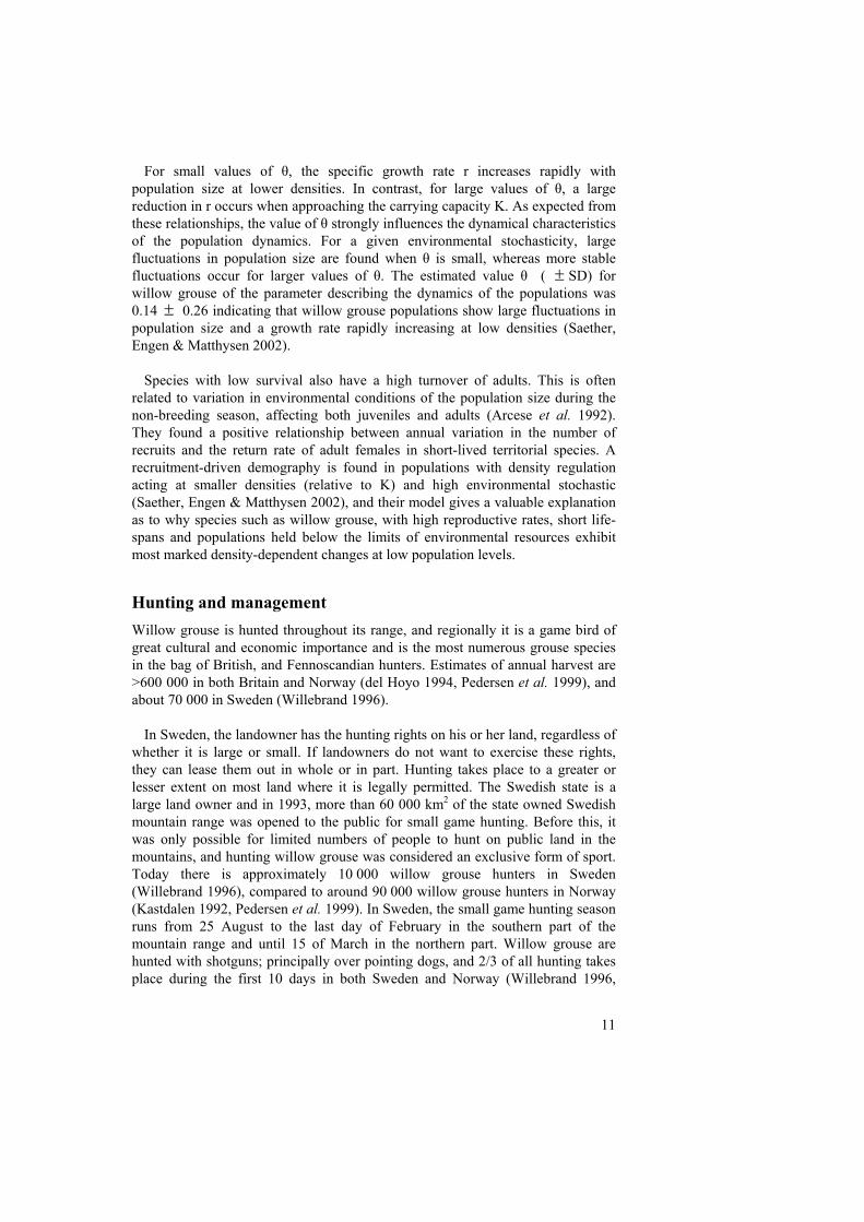
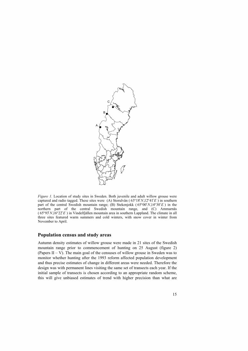
in the Swedish mountain range (Paper IV). These sites were (A) southern part of the central Swedish mountain range (Storulvån 1992 – 1995, EN 1412,8163 ′°′° ); (B) Stekenjokk mountain area (Stekenjokk 1998 – 1999, EN 0314,0065 ′°′° ) in the northern part of the central mountain range; (C) Vindelfjällen mountain area in southern Lapland (Ammarnäs 1997 – 1998, EN 2216,3965 ′°′° ) (figure 1). Storulvån contained of three subunits; one hunted site where hunters were intensively monitored, and two control sites where hunting was forbidden. Ordinary willow grouse hunting was allowed outside the study sites. My other two study sites were hunted from 25 August to the last day of February in Stekenjokk and in Ammarnäs hunting was permitted until 15 March. During the whole study more than 300 willow grouse were captured and fitted with radio-transmitters. Three different methods were used to capture grouse depending on season. Between late July and mid August we caught adults and their chicks prior to brood break-up by using pointing dogs to locate the birds

13

14

which then were flushed into nets. During winter and early spring, birds were trapped in walk-in cages or spot-lighted and netted during night.

Individual grouse were aged based on their primary feather pigmentation (Bergerud, Peters & McGrath 1963) and classified as juveniles (< 1 year) or adults. Weight, wing-length and secondary sexual characteristics were recorded in order to sex adult birds. Willow grouse chicks were sexed using DNA probes in site A while chicks caught in the other two sites were flushed several times during their lifetime to be sexed by morphological signs and behavioral patterns. All caught birds were marked with wing-tags (Höglund 1956), and birds weighing over 300 g, fitted with a small radio transmitter (Holohil Systems, Ltd., Ontario, Canada) of 7 – 13 g with an lifetime of 14 – 28 months.

Grouse locations were obtained by telemetric triangulation using hand-held 3-element Yagi antennas and radio receivers and portable GPS receivers (Garmin) were used to give observer location and/or grouse positions when flushed. Birds were checked more frequently during August to October and March to the beginning of June. Birds were not checked between mid-December and mid January in any site any year because weather and snow conditions made it difficult to reach the study sites. During dispersal periods in spring and autumn aircraft were used to locate long distant dispersers to a maximum distance of 40 km. Aerial tracking was accomplished as described in Samuel & Fuller (1994). Attempts to visually locate birds were made as soon as possible following dispersal, and in most cases birds were located within a week after dispersal. The radio-transmitters had mortality functions on and when a bird’s radio signal indicated mortality, it was visually located and checked.

Since uneven tracking schedules were used in the different sites, data from the least intensively tracked site determined my choice of distance measurement. I divided the year into two periods; summer (May – August) and winter (September – April). This also reflected the changes in weather conditions and grouse biology. I estimated natal dispersal distances for complete dispersers as the maximum distance moved from first summer caught to next summer. I used the straight-line maximum distance between time periods since I could not precisely define the natal area or the home range of all the parents. All willow grouse that dispersed from natal areas tended to disperse rapid and abrupt, in a strait line (Smith 1997). Rapid movements sometimes continued for a period of several days interspersed with periods when grouse were more sedentary during the rest of the period. The same procedure with the straight-line maximum distance between time periods was used when calculating movement of adult birds.

15

#

#

#

A

B

C

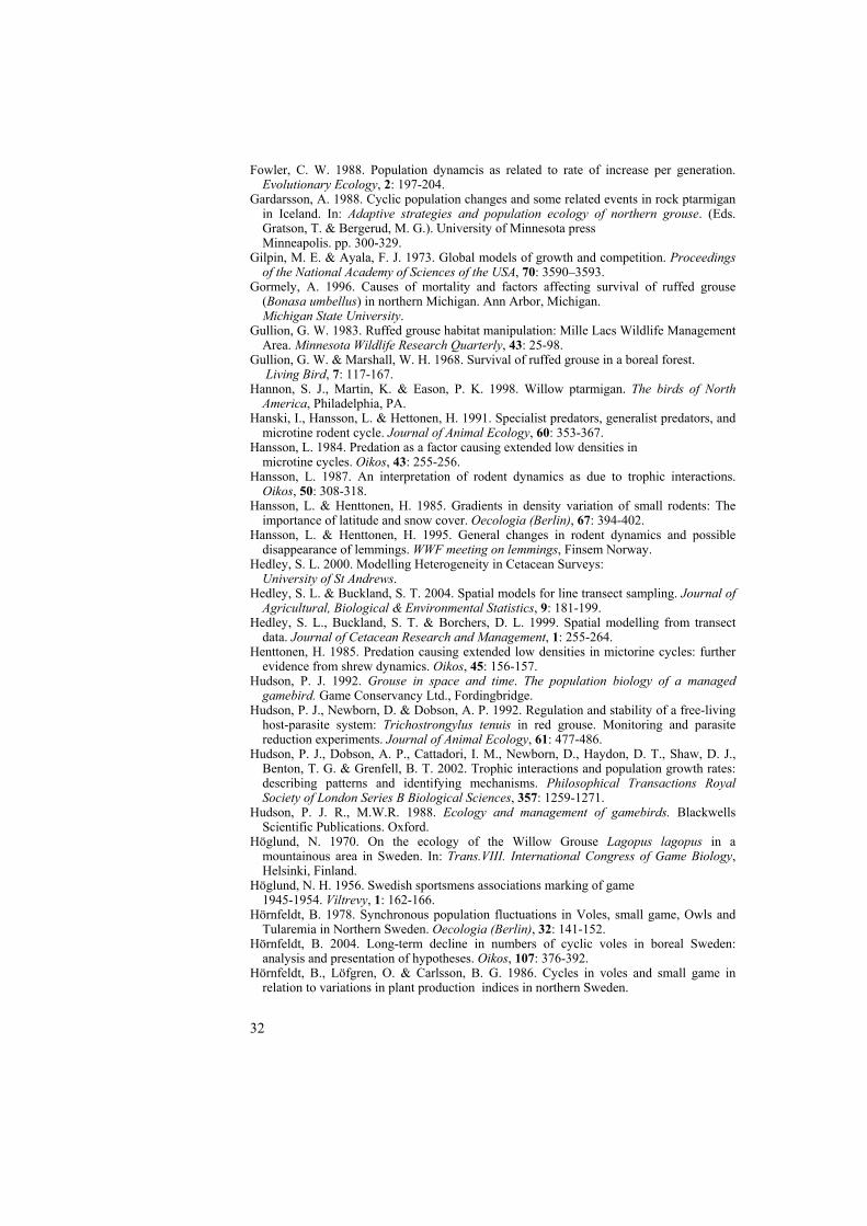
Figure 1. Location of study sites in Sweden. Both juvenile and adult willow grouse were captured and radio tagged. These sites were (A) Storulvån ( EN 1412,8163 ′°′° ) in southern part of the central Swedish mountain range; (B) Stekenjokk ( EN 0314,0065 ′°′° ) in the northern part of the central Swedish mountain range, and (C) Ammarnäs ( ) in Vindelfjällen mountain area in southern Lappland. The climate in all three sites featured warm summers and cold winters, with snow cover in winter from November to April.

EN 2216,3965 ′°′°

Population census and study areas Autumn density estimates of willow grouse were made in 21 sites of the Swedish mountain range prior to commencement of hunting on 25 August (figure 2) (Papers II – V). The main goal of the censuses of willow grouse in Sweden was to monitor whether hunting after the 1993 reform affected population development and thus precise estimates of change in different areas were needed. Therefore the design was with permanent lines visiting the same set of transects each year. If the initial sample of transects is chosen according to an appropriate random scheme, this will give unbiased estimates of trend with higher precision than what are

obtained by selecting new transects each year (Thomas, Burnham & Buckland 2004).

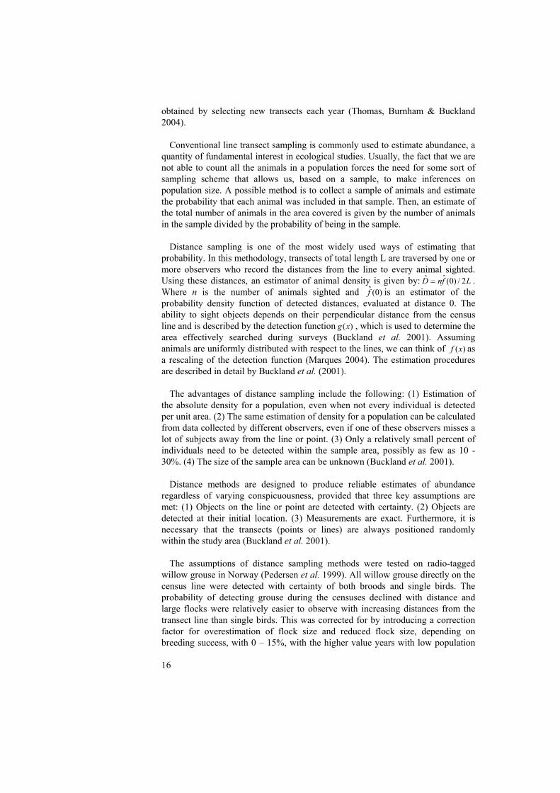
Conventional line transect sampling is commonly used to estimate abundance, a quantity of fundamental interest in ecological studies. Usually, the fact that we are not able to count all the animals in a population forces the need for some sort of sampling scheme that allows us, based on a sample, to make inferences on population size. A possible method is to collect a sample of animals and estimate the probability that each animal was included in that sample. Then, an estimate of the total number of animals in the area covered is given by the number of animals in the sample divided by the probability of being in the sample.

Distance sampling is one of the most widely used ways of estimating that

probability. In this methodology, transects of total length L are traversed by one or more observers who record the distances from the line to every animal sighted. Using these distances, an estimator of animal density is given by: . Where n is the number of animals sighted and is an estimator of the probability density function of detected distances, evaluated at distance 0. The ability to sight objects depends on their perpendicular distance from the census line and is described by the detection function , which is used to determine the area effectively searched during surveys (Buckland et al. 2001). Assuming animals are uniformly distributed with respect to the lines, we can think of as a rescaling of the detection function (Marques 2004). The estimation procedures are described in detail by Buckland et al. (2001).

LfnD 2/)0(ˆˆ =)0(f̂

)(xg

)(xf

The advantages of distance sampling include the following: (1) Estimation of

the absolute density for a population, even when not every individual is detected per unit area. (2) The same estimation of density for a population can be calculated from data collected by different observers, even if one of these observers misses a lot of subjects away from the line or point. (3) Only a relatively small percent of individuals need to be detected within the sample area, possibly as few as 10 - 30%. (4) The size of the sample area can be unknown (Buckland et al. 2001).

Distance methods are designed to produce reliable estimates of abundance regardless of varying conspicuousness, provided that three key assumptions are met: (1) Objects on the line or point are detected with certainty. (2) Objects are detected at their initial location. (3) Measurements are exact. Furthermore, it is necessary that the transects (points or lines) are always positioned randomly within the study area (Buckland et al. 2001).

The assumptions of distance sampling methods were tested on radio-tagged willow grouse in Norway (Pedersen et al. 1999). All willow grouse directly on the census line were detected with certainty of both broods and single birds. The probability of detecting grouse during the censuses declined with distance and large flocks were relatively easier to observe with increasing distances from the transect line than single birds. This was corrected for by introducing a correction factor for overestimation of flock size and reduced flock size, depending on breeding success, with 0 – 15%, with the higher value years with low population

16

17

size and high breeding success. The corrected value is calculated using a linear regression between flock size and distance from census line and corrects for an increase in flock size with distance from the census line (Buckland et al. 2001). A test was also carried out to investigate the activity of the birds when using hunting dogs and assess whether birds were detected at their initial locations. The general pattern was that grouse were more active when the census team was far away, becoming more passive as the team got closer (Pedersen et al. 1999). Evaluation of the accuracy of the paced out distances were made in one site between 1999 – 2004 by letting the observers both measure the perpendicular distance both by tape measure and by pacing out, and no significant difference between detection functions and estimate of densities between the two methods of measuring distances was found (M. Hörnell-Willebrand unpubl. data). The variation (% CV) around the estimates are between 10-30% and most of this variation is due to variation in number of grouse in the different transects.

The half-normal, hazard rate, negative exponential and uniform models (with and without cosine series expansion) were fitted to the data. The best model was selected with the use of Akaike’s Information Criterion (AIC) (Akaike 1973) and a corresponding density for each site and year was estimated by using program DISTANCE (Thomas et al. 2003). Due to small sample sizes in low density years, I modeled the entire data set in each site and stratified by year. Models used by program DISTANCE are “pooling robust” to variation in detection probability and stratification will improve precision and reduce bias of estimates when detection patterns vary among years (Buckland et al. 2001).

####

####

# #

#

#

##

#

####

##

%U

%U

%U

%U

%U

%U

# Norrbotten

# Västerbotten

#

Jämtland

# 2324

#

6789

#

45

#

23

#22

# 20#

19

#

21 #

17#

16#

18

#11

#

12#

10

#15

#13#

79#

89

#

99 #

1

SWEDENNORWAY

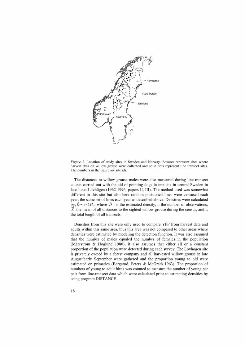
Figure 2. Location of study sites in Sweden and Norway. Squares represent sites where harvest data on willow grouse were collected and solid dots represent line transect sites. The numbers in the figure are site ids.

The distances to willow grouse males were also measured during line transect

counts carried out with the aid of pointing dogs in one site in central Sweden in late June: Lövhögen (1962-1996, papers II, III). The method used was somewhat different in this site but also here random positioned lines were censused each year, the same set of lines each year as described above. Densities were calculated by; LxnD 2/ˆ = , where is the estimated density, n the number of observations, D̂x the mean of all distances to the sighted willow grouse during the census, and L the total length of all transects.

Densities from this site were only used to compare YPP from harvest data and adults within this same area, thus this area was not compared to other areas where densities were estimated by modeling the detection function. It was also assumed that the number of males equaled the number of females in the population (Marcström & Höglund 1980), it also assumes that either all or a constant proportion of the population were detected during each survey. The Lövhögen site is privately owned by a forest company and all harvested willow grouse in late August/early September were gathered and the proportion young to old were estimated on primaries (Bergerud, Peters & McGrath 1963). The proportion of numbers of young to adult birds was counted to measure the number of young per pair from line-transect data which were calculated prior to estimating densities by using program DISTANCE.

18

19

Time-series analysis Six long time-series of harvest data were used during this study (three from Sweden (S) and three from Norway (N): 1. Lövhögen, S (1962-1996), 13. Ammarnäs, S (1960-1996), 15. Arjeplog, S (1974-1997), 79. Hattfjelldal, N (1967-2003), 89. Grane/Vefsn, N (1967 – 2003), and 99. Östre Slidre, N (1979-2003) (figure 2). Grouse were aged depending on coloration and pattern of molt (Bergerud, Peters & McGrath 1963). From this data I determined the number of young to adult birds in the shot samples and investigated the pattern of cyclicity and correlation (Paper II).

The investigation of time-series, a chronological collection of population estimates, has been central to the understanding of population dynamics (Turchin 2003). Game records analysis with the aid of time-series started early in Europe (Siivonen 1948, Moran 1952), and different features of many populations have been investigated in Fennoscandian populations (Hörnfeldt 1978, Hansson & Henttonen 1985, Marcström, Höglund & Krebs 1990, Angelstam, Lindström & Widén 1985, Myrberget & Lund-Tangen 1990, Ranta et al. 1997).

Traditional time-series analyses are done by breaking down (decomposing) the variance of a time series into a trend, seasonal variation, other cyclic oscillations, and the remaining irregular fluctuations (Chatfield 1989). The ultimate aim of a time series analysis of population dynamics is to construct mechanistic models to investigate the population processes (Kendall et al. 1999, Turchin 2003). Measures of population are often log transformed prior to any analysis when transformation helps to stabilize the variance and translates multiplicative population processes into linear, additive, effects more amiable to statistical analysis Turchin 2003).

A trend is a long-term, exogenously driven systematic change in the population and is most often represented in time-series by a change in the mean level of fluctuations. The probability theory of time series analysis is based on the assumption that time series are stationary (mean and the variance is constant), and trends violate this stationarity assumption. The most widely used approach is to model the trend and use the residuals in the time series (Turchin 2003). Removing a linear trend involves regressing Y=log Nt on time to obtain intercept and slope. Non-linear trends can be removed by fitting higher order polynomials but the use of polynomials can be questioned as polynomial regression is rather inflexible and constrains the output. A more flexible way is to use a locally weighted polynomial regression (LOESS), which is a non-parametric form of regression that fits a polynomial surface using local fitting (Cleveland 1979, Cleveland & Devlin 1988).

Long time-series are needed when investigating second-order dynamics that tend to yield lower frequency oscillations (6-12 years). For investigating first-order dynamics, which tend to exhibit higher frequency oscillations, a shorter time-series may be sufficient. A general rule of thumb is that the time-series

20

should represent 3 data points, which are three complete oscillations (Turchin 2003).

Autocorrelation Function (ACF) is used to detect periodicity in time series data. Autocorrelation measures the degree of association between numbers in a time series separated by different time lags. The autocorrelation between the logarithms of population counts separated by one time lag is obtained by calculating the coefficient of correlation between log Nt and log Nt-1 over the entire series. This is called the autocorrelation at lag 1. The auto-correlation for lag two is the correlation between log Nt and log Nt-2. Plots of autocorrelation coefficients are plotted against their lag to give the autocorrelation function (ACF). Examination of the ACF also allows an objective estimate of the dominant cycle period (Turchin 2003). The dominant period of a cycle, T, can be identified by finding the lag at which ACF reaches its first maximum, and this point is termed ACF(T). We can test whether this is significantly different from zero by applying Bartlett’s criterion ACF(T) > 2/√n, where n is the length of the time-series (Royama 1992). If ACF(T) exceeds Bartletts’s criterion there is strong evidence of statistical periodicity. If ACF(T) is smaller then we check the ACF at the lag nearest half the estimated period and if ACF(T/2) < -2/√n then there is weak evidence of statistical periodicity. If neither ACF(T) nor ACF(T/2) are significant there is no evidence of periodicity.

The determination of the process order is fundamental to time-series analysis. While, ACF is a useful tool for identifying the period of a time-series it does not give much information about the dimension or structure of density-dependant processes. To overcome this limitation of ACF, Box & Jenkins (1976) proposed the use of partial autocorrelation coefficients as an indicator of the order of the process. The partial autocorrelation shows the correlations between Nt and Nt-d, where d is a time lag, with the effect of earlier lags removed by inclusion of the regression residuals from earlier lags. Partial autocorrelations are plotted against lag to give the partial autocorrelation function (PACF). PACF is used to identify a candidate value for the number of lags needed to model the population fluctuations: the process order; which is the number of lagged densities affecting the realised per capita rate of change. First-order oscillations are systems in which population feedbacks operate with time lags of one generation or less, typical periods are in the range of 2-3 generation times, and population declines can be rapid and take place in one time step. A second-order oscillations are driven by feedbacks that operate over time lags of more than one generation and give rise to cycles of 6-12 years. In second-order processes population declines usually take place over more than one time step. (Turchin 2003).

PACF is not well suited to detecting negative feedback at lag one because of positive autocorrelations due to reproduction, which can mask any negative feedback (Berryman 1992, Berryman & Turchin 2001, Turchin 2003) . The solution, which is similar to the approach used in phase-plots, is to regress Rt=log (Nt/Nt-1) against lagged log-population density whilst controlling for the affect of previous population density. This provides the partial correlations between the per-capita rate of change Rt, and lagged population density Nt-d and gives, the

21

partial rate correlation (PRCF) (Turchin 2003). The PRCF provides better information than PACF on the lag structure of the negative feedback mechanisms acting on the population at lag one. Note that PRCF at lag two or greater is the same as PACF at the same lag. This means that an investigator only needs to calculate PRCF(1) = correlation Rt vs. log Nt-1. PRCF(>lag 1) is the same as the corresponding PACF at the same lag.

Cross-correlation is a method that can be used to investigate the correlation in time-series between populations. Cross-correlation plots help to identify relations between two different series and any time delays to the relations. A correlation for a negative lag indicates the relation of the values in the first series to values in the second series that number of periods earlier. The correlation at lag 0 is the usual Pearson correlation. Similarly, correlations at positive lags relate values in the first series to subsequent values in the second series.

Results and discussion

Population dynamics and density-dependence (II, III) Time series of breeding success from populations indexed in late August by direct counts showed a spatial correlation between sitess up to 200 km apart, indicating that external agents synchronize the average young per pair in the populations (paper II). However, there was no spatial correlation of adult density indicating that this synchronizing agent must act during spring and summer. The results from paper III showed significant positive, non-significant and even significant negative relationships between breeding success and intrinsic rate of increase. There was a positive relationship in the northernmost region where first and second order density dependence was found to be weak and of equal strength, but no relationship was found in the southernmost region where density dependence was stronger and dominated by a first order density dependence. The study sites showed average adult densities in August (2.4 – 8.2 adults/km2). Strong first order density dependence would be expected to smooth large variations in fall populations until next spring. We did not find any evidence of adult density affecting chick production from the 21 sites where population densities were measured by direct counts. We found little evidence of cyclic fluctuations in either the adult populations or chick production in the long time-series of harvest data from Sweden and Norway, or from willow grouse populations indexed by direct counts in Sweden. Lindström et al. (1995) used the term clock-work for the population fluctuation of the Finnish woodland grouse and Steen et al. (1988b) suggested that the chick production of willow grouse varied with such regularity that it could be a used to predict good and bad years in grouse management. Our findings suggest that the regular periodicity in chick production is rather an exception than a rule in willow grouse.

It has long been known that the harvest data of willow grouse from Sweden and Norway produce almost identical long term averages in chick production with a

22

long term average of about 2.8 young per pair. We found that breeding success from sites based on transect counts of willow grouse varied to a much larger extent with a significantly higher grand mean than the average breeding success from harvest data, with a difference of more than one young per pair (3.99 compared to 2.88). The differences between the data sets were more apparent at higher breeding success and we suggest that the harvest process in itself acts to adjust the young to old ration in the bag to a similar distribution in different areas.

Thus, my observations do not find a solution to the puzzle of why populations cycles, other than the Swedish willow grouse populations fluctuations, seems to be less regular than previous showed or believed. The overwhelming majority of examples of populations oscillations in nature are explained by the mechanism of specialist predation (including parasitoids), and I found this explanation to be the most plausible even in the regulation of willow grouse populations. I suggest that the density dependent mechanism is caused by predation during winter and early spring but that on the local scale, dispersal evens out density differences and makes compensatory mortality difficult to detect.

Willow grouse exhibit different dynamical pattern in the southern and in the

northern part of the Swedish mountain range, suggesting that the mechanisms underlying these fluctuations can be quite variable. Future research should strive to investigate the demographic mechanisms at very low density levels of willow grouse populations, and try to find out whether, or to what extent, over winter mortality does or does not compensate for hunting. This could be done by reducing populations close to extinction and then measuring immigration, breeding success and mortality.

Movements and dispersal (IV) Large-scale spatial dynamics are difficult to study (Taylor 1990), and dispersal in many cases has been overlooked as an important factor in local population dynamics, characterized as source-sink systems such as willow grouse population dynamics. Paper IV is the first study to provide evidence for a general pattern of seasonal and age related movements in willow grouse.

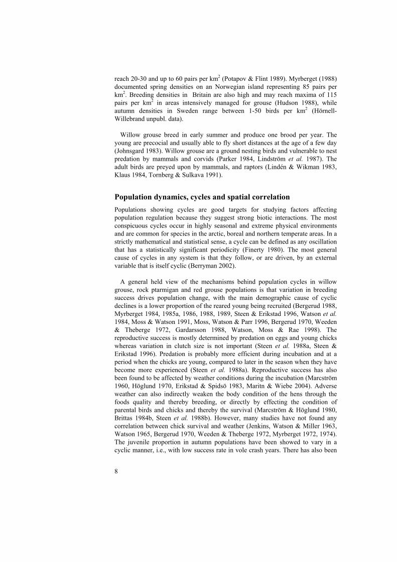
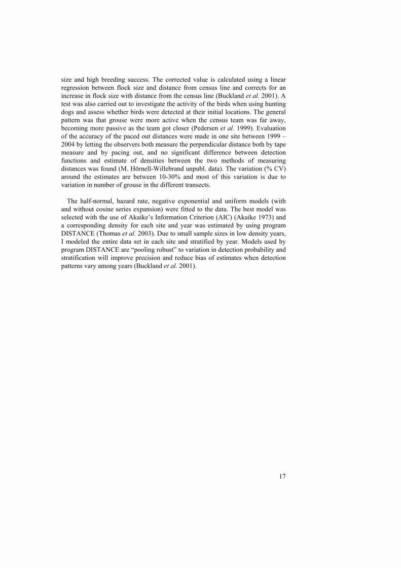
Figurejuvenigrousesummkm).

We

male distanjuvenof thenatal similaappardistandifferdisper

1 2 3 4 5 6 7 8 9 10 15 16-20 > 21

FemalesMales

Natal Dispersal

02

46

8 a)

1 2 3 4 5 6 7 8 9 10 15 16-20 > 21

Summer to Winter

Freq

uenc

y

010

2030 b)

1 2 3 4 5 6 7 8 9 10 15 16-20 > 21

Winter to Summer

Distance

010

2030 c)

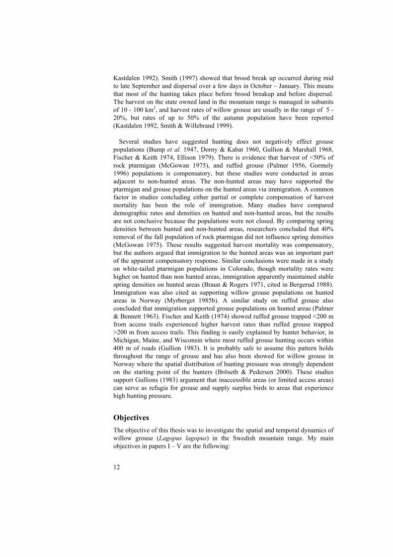
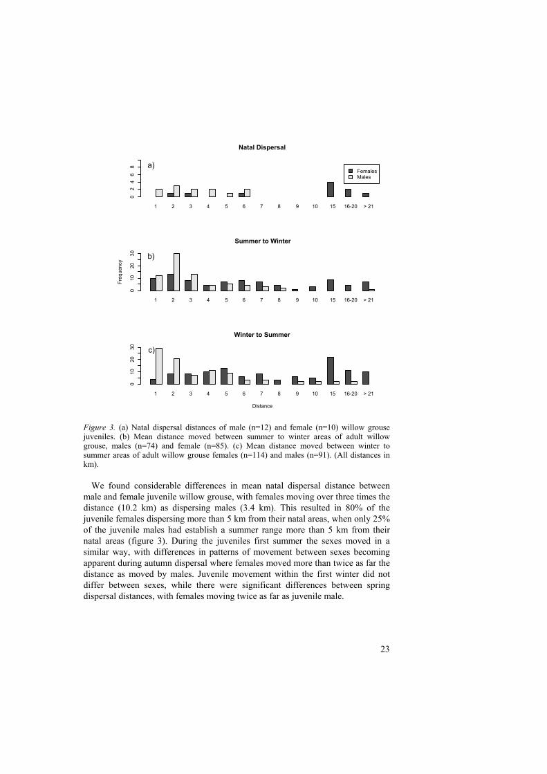
3. (a) Natal dispersal distances of male (n=12) and female (n=10) willow grouse les. (b) Mean distance moved between summer to winter areas of adult willow , males (n=74) and female (n=85). (c) Mean distance moved between winter to er areas of adult willow grouse females (n=114) and males (n=91). (All distances in

found considerable differences in mean natal dispersal distance between and female juvenile willow grouse, with females moving over three times the ce (10.2 km) as dispersing males (3.4 km). This resulted in 80% of the ile females dispersing more than 5 km from their natal areas, when only 25% juvenile males had establish a summer range more than 5 km from their areas (figure 3). During the juveniles first summer the sexes moved in a r way, with differences in patterns of movement between sexes becoming ent during autumn dispersal where females moved more than twice as far the ce as moved by males. Juvenile movement within the first winter did not between sexes, while there were significant differences between spring sal distances, with females moving twice as far as juvenile male.

23

24

There were no differences in movement patterns between the three areas, and adult movements were similar to that of juveniles. Adult females moved further from the area where they nested and raised broods to over-wintering sites than males, and almost all females (82%) returned to the area where they nested and raised broods the previous year (figure 3).

We did observe dispersals as long as 25 km made by some males, and though most male willow grouse remained in their area of birth, 25% did move more than 5 km. This can explain why analyses of genetic similarity among willow grouse revealed no significant difference between males and females (Rörvik, Pedersen & Steen 1998) which would be expected if no males moved as previously thought. The long term effects of accumulated short dispersal distances of individuals can be remarkably successful in expanding the distribution of a population.

An important question is to what extent this rate and sex differences in movement patterns found in our study, is modified by changes in local density. We were unable to detect any differences between years or areas, although the hunting pressure ranged from no hunting to harvest rates exceeding 60%, suggesting that the population levels differed between areas and years. As a working hypothesis we suggested that the high proportion of juvenile males that remain and juvenile females that leave are independent of local population size, but that local density is a cue that affects where the dispersal will end. Thus, juvenile emigration is probably not density-dependent while this effect does operate on immigration.

Our findings can be part of the explanation to why several studies of harvest willow grouse populations have not found a decrease in heavily hunted areas compared to areas with no harvest. The non-hunted areas may have supported populations on hunted areas via immigration. One possible reason for the disparities among the effects of grouse harvest is that dispersal and compensatory mortality might interact to induce regional synchrony over large areas. If these processes occur in the same time, but dominate on different scales, it will be difficult to measure the effects of dispersal and compensatory mortality separately. Thus, this problem has to be carefully addressed in further studies of willow grouse population dynamics.

Management and harvest (I, V) In paper I, we used a spatial model of a fluctuating population of willow grouse to investigate the possible advantages of buffer zones in managing harvest. The outcome of our model was investigated under four different scenarios and our analysis suggests that the use of buffer zones may provide a simple strategy for managing the harvest of our stochastic model population. About 75% of the area could be left open to hunting even if the level of harvest was close to the extinction level if executed in all grids. The management system would only need to ensure that the refuges are not utilized once the required size and distribution of buffers are established. However, our model acts on such a large scale that it

would be difficult in traditional experimental research. The assistance of managers willing to adopt harvest strategies that provide data to compare different models would be a more fruitful approach.

25

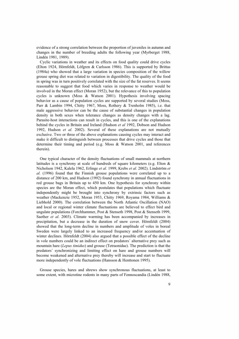
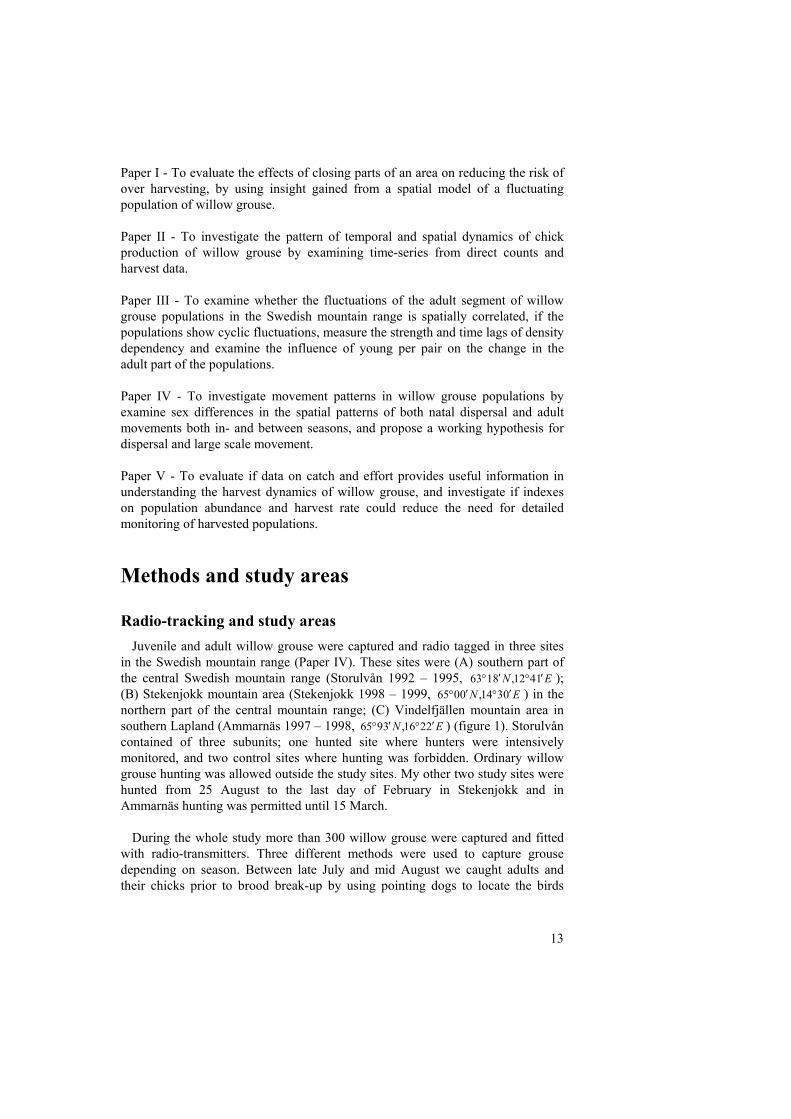
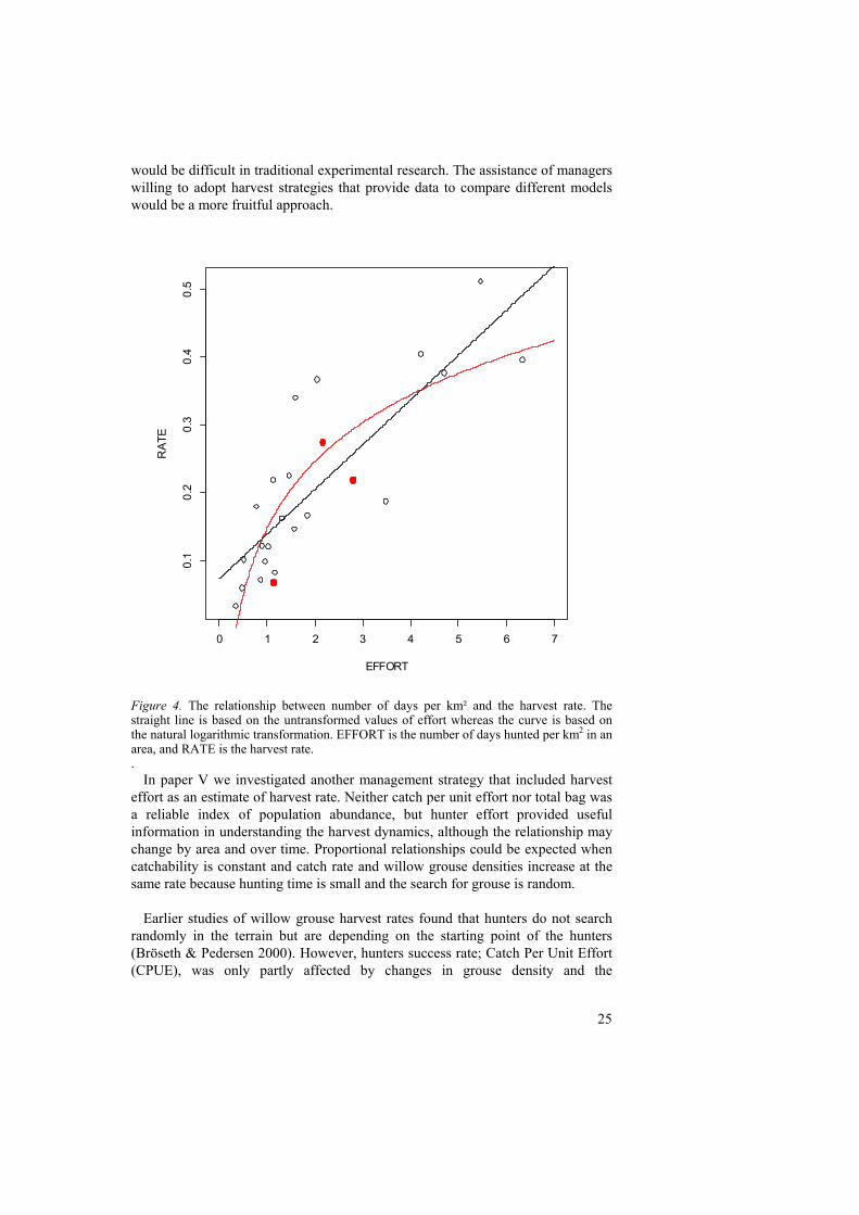
Figure 4. The relationship between number of days per km² and the harvest rate. The straight line is based on the untransformed values of effort whereas the curve is based on the natural logarithmic transformation. EFFORT is the number of days hunted per km2 in an area, and RATE is the harvest rate.

0 1 2 3 4 5 6 7

0.1

0.2

0.3

0.4

0.5

EFFORT

RA

TE

. In paper V we investigated another management strategy that included harvest

effort as an estimate of harvest rate. Neither catch per unit effort nor total bag was a reliable index of population abundance, but hunter effort provided useful information in understanding the harvest dynamics, although the relationship may change by area and over time. Proportional relationships could be expected when catchability is constant and catch rate and willow grouse densities increase at the same rate because hunting time is small and the search for grouse is random.

Earlier studies of willow grouse harvest rates found that hunters do not search

randomly in the terrain but are depending on the starting point of the hunters (Bröseth & Pedersen 2000). However, hunters success rate; Catch Per Unit Effort (CPUE), was only partly affected by changes in grouse density and the

26

catchability increased as the population decreased. Increased catchability has also been found in recreational fishery at lower densities of lake trout (Post et al. 2002). This depensatory mortality in combination with high catch rates could reduce a population below a critical level of depensation where it would inevitable go extinct. A fundamental question is whether catchability of willow grouse continues to increase as populations decline, or if a threshold is reached where hunter success begins to decline (figure 4). We conclude that the annual accumulated effort can be a valuable tool in harvest management of small game. Setting limits to the totally allowable effort within an area has probably more potential for controlling harvest of small game than daily bag limits and adjusting the length of the open season.

Conclusions

The pattern of population dynamics showed a large variation in the different areas where I studied willow grouse. It does not suggest different ecological mechanisms but rather that the local settings for the willow grouse are different, and thereby creating a varied pattern of fluctuations. The challenge is to find the principles of the mechanisms that create these patterns. I have shown that willow grouse populations in the Swedish mountain range only showed weak evidence of cyclic fluctuations, both in breeding success and the adult segment of the population. The weak secondary density dependence in the north fit well with the general theory of less generalist predators, which are more common in the southern mountain range. However, there seem to be a general trend of increasing number of generalist predators as red fox and mink higher up in the mountains and further north, possibly due to global warming. I suggest that the occurrence of regular cycles will probably be less likely although the large fluctuations may well persist.

Breeding-success showed a spatial correlation between sites up to 200 km apart, while there was no correlation in the adult populations between sites. The number of adults in the population did not show any relationship with breeding success, and I believe that the annual variation in breeding success is probably affected by a combination of predators, food quality of females during egg-laying and weather. The alternative prey hypothesis is likely to be the most dominating mechanisms in areas where microtines show strong cyclic pattern, in other areas predation rate is probably affected more by random events such as weather. The different sites also seemed to vary more in average breeding success than in average adult density, showing that although breeding success is not density dependent it is probably affected by local features.

The adult part of the population varied to a lesser extent than the breeding success although the extent of the annual variation in number of adults seems to be tied to local landscape conditions. The poor spatial correlation but density-dependent changes in the adult population suggest that it is local conditions determining these fluctuations. Since I only have measurement of the population

27

in summer I cannot determine if the changes are due to losses in winter or in spring and early summer.

I have shown that the dispersal pattern of willow grouse follow the general pattern of birds, and most juvenile females will move into new populations before breeding. Juvenile males, on the other hand, mostly remain in their natal population. I suggest that one reason for the disparities among the effects of grouse harvest is that dispersal and compensatory mortality might interact over large areas. If these processes occur at the same time, but dominate on different scales, it will be difficult to measure the effects of dispersal and compensatory mortality separately.

My results show that conclusions from harvest statistics have to be treated with caution. Hunters bag young grouse disproportionately to what is present in the population, resulting in a long term average that underestimates the true value and conforms the distribution of young per pair to be same in different areas. Catch per unit effort showed a poor correlation with population abundance, and the catchability increased as the population decreased. However, I found that the proportion harvested was almost constant in the area with restricted access to local hunters, and here the total bag could be used to index population abundance. I showed that harvest effort can be a valuable tool in harvest management of willow grouse in the open access system on state land since it shows a good relationship with harvest rate. I also suggest that that using unhunted buffer zones can secure a sustainable harvest without the need for a resource demanding control system. This harvest management strategy is especially well suited where managers have control over large areas such as the state owned land in the Swedish mountain range.

Future research

My results have highlighted several areas that I feel require further investigation. Obviously the time series from the 21 line transects sites will become more valuable as time progress. It will be possible to compare the different sites in a more rigorous way, and further investigate possible gradients and outliers in the patterns of density dependency. I believe that it is interesting to establish if there is a north to south gradient and to further study the two sites in the central mountain range that departed markedly from the other sites. It will also be important to further evaluate the use of harvest data in management.

However, there is also a need for a more experimentally manipulative approach, and I suggest that the strength and mechanisms of density dependence should be investigated by reducing an isolated population of willow grouse close to extinction, and then measure immigration, breeding success and mortality. The willow grouse population living on the isolated mountain area Dundret in Norrbotten would be suitable for an experiment of this kind, since Dundret is

28

separated from other high quality willow grouse habitat, and population densities of willow grouse in surrounding forested areas are expected to be low.

My research has generated a lot of data of grouse locations with or without radio transmitters, and with the new technology available in GIS and remote sensing I believe there are many questions that can be answered regarding habitat preferences and spatial distributions using both density and breeding success as dependent variables. Habitat variables from willow grouse could be mapped in all study sites when all positions during the years have been positioned with portable GPS receivers. This could be done by estimating willow grouse density, breeding success and potentially survival as a function of location, allowing for those parameters to be related to habitat or other location covariates. These methods also enable estimation of abundance for any sub area of interest within the surveyed region. Methods have been developed to relate animal density to spatial variables that affect the animals´ environment (Hedley 2000, Hedley, Buckland & Borchers 1999), and more statistical techniques are under development (Hedley & Buckland 2004), but they have yet been applied to willow grouse populations.

Climate change impacts strongly on wildlife species at high elevations (Burton 1995, Jenik 1997, Inouye et al. 2000), and higher temperatures have the potential to alter the amount of alpine and sub-alpine habitat and to increase alpine fragmentation because of rising sub-alpine treelines (Roland, Keyghobadi & Fownes 2000, Martin 2001). Long-term monitoring programs for alpine and sub-alpine wildlife, like the Swedish willow grouse census, will have high efficiency when even small increments in warming are shown to significantly impact habitat quantity and quality for breeding and migration in other Lagopus species (Martin 2001). Models show that temperature increases of only 3-5 oC, well within the ranges predicted under global warming, could have serious implication for the alpine tundra habitat. To detect and predict the ecological effects of global climate change, it will be crucial to continue with the willow grouse census in Sweden.

Maybe most intriguing path forward would be to continue to investigate the affect on hunter anticipation and behavior on catch rates and effort in relation to population abundance. I believe that it is possible to merge traditional predator-prey theory with the insights gained from the rapidly advancing discipline “Human dimensions of wildlife”. There is an obvious gap in our knowledge about hunter expectations and the values forming their behavior, and we expect different patterns will develop along the axis of open access to highly restricted, from day permits to long term lease and a strong commitment to the land.

Finally, and even if the above suggestions are not addressed, I believe that there are sufficient results to synthesize the available knowledge into a broad understanding of the dynamic of willow grouse. This will identify the important gaps in the understanding of willow grouse and could be formulated in to a number of competing models. The management of small game on the state owned land in Sweden is well suited to incorporate and test these competing models by developing an adaptive management plan.

29

Acknowledgements

First of all, I want to thank my supervisor professor Kjell Danell for giving me the opportunity to work on this fascinating aspect of ecology that is the population dynamics of willow grouse. He has supported me during the whole process of my postgraduate studies and has also shared his wide knowledge of ecology. His commitment to good science will always be an inspiration. Then, I want to thank Tomas Willebrand who originally set up the willow grouse project, employed me to catch willow grouse and ended up as my husband. Tomas’ input, advice and support have been central to the success of the willow grouse project.

This work had not been possible without the help of the Swedish grouse hunters. They have made a tremendous contribution in censusing willow grouse thought the years; it is thanks to you the Swedish willow grouse census have this high international standard. I also want to thank the Swedish Hunters Association and the county boards in Jämtland, Norrbotten and Västerbotten for supporting the grouse census.

Much of the data used in this report was kindly contributed by Vidar Marcström, Rolf Brittas and Martin Håker. Without help in the field of my “field-girls”; Angelika Hammarström, Sara Edfalk, Erika Edfors and Rosalyn Schumacher, there had been no willow grouse to write about. I am very grateful to Jan-Peter Magnusson and Erik Ringaby for their skilful work with their dogs during the grouse catching in the summers. Thanks for sharing your companionship during sometimes rough field conditions. I also want to thank all my colleagues at the Department of Animal Ecology at the Swedish University of Agricultural Sciences, Umeå for creating a productive scientific environment and stimulating scientific environment.

Thanks are due also to several other people during this study: Lasse Strömgren at the research station in Ammarnäs for making things going smoothly and making my staying at the pleasant, the Sámi villages working with reindeer husbandry in my study sites for good cooperation, Macke and Inger Långström at Blåsjöns Fjällcamp for all support and encouragement and Scott Newey for providing valuable feedback on the manuscripts. I am also grateful to Christopher Heap who provided valuable suggestions to improve the language of this thesis, and I am thankful to all my coo-authors for working with me on the manuscripts. I am grateful to the very helpful secretary at Fjäll-MISTRA, Ylva Johansson for supporting me with all the administrative work before finalizing the dissertation. A big hug to you Ylva, for running everything so smoothly and for assisting me in many different ways.

30

This project was financed by the Swedish Hunters Association, the Swedish Environmental Protection Agency and the MISTRA foundation. Permits to capture and handle grouse were given by the Swedish Environmental Protection Agency. All handling of animals in the study followed the principles and guidelines set out by the Swedish National Board for Laboratory Animals.

My deepest appreciation is for my families, who have shown me nothing but encouragement, understanding and love. Special thanks to my parents and to my mother in law, that have spent weeks and weeks babysitting and given me the space to work. Without your help finishing this thesis would have been a lot harder.

Lastly, and most importantly, I wish to thank my entire extended family for providing a loving environment for me. My children Anders and Signe, for their joy and inspiration, my beautiful and intelligent “bonus-children”; Kerstin, Elsa and Sofia – I thought teen-agers like you only existed in the fairytales, and my husband Tomas for sharing my life. To them I dedicate this thesis.

References

Abrahamsen, J., Jakobsen, N. K., Dahl, E., Kalliola, R., Wiborg, L. & Påhlson, L. 1977. Naturgeografisk regionindelning av Norden (in Swedish). Nordiska utredningar, Stockholm. Sweden. (In Swedish).

Akaike, H. 1973. Information theory and an extension of the maximum likelihood principle.In: International Symposium on Information Theory, 2nd edn. (Eds. Petran, B. N. & Csaaki, F.). Akadèemiai Kiadi. Budapest, Hungary.

Angelstam, P., Lindstrom, E. & Widen, P. 1984. Role of predation in short term population fluctuations of birds and mammals in Fennoscandia. Oecologia, 62: 199-208.

Angelstam, P., Lindström, E. & Widén, P. 1985. Synchronous short-term population fluctuations of some birds and mammals in Fennoscandia - occurrence and distribution. Holartic Ecology, 8: 285-298.

Arcese, P., Smith, J. N. M., Hochachka, W. M., Rogers, C. M. & Ludwig, D. 1992. Stability, regulation, and the determination of abundance in an insular song sparrow population. Ecology, 73: 805-882.

Bergerud, A. T. 1970. Population dynamics of the willow ptarmigan Lagopus lagopus alleni L. in Newfoundland 1955 to 1965. Oikos, 21: 299-325.

Bergerud, A. T. 1988. Population ecology of North American Grouse. In: Adaptive Strategies and Population Ecology of Northern Grouse. (Eds. Bergerud, A. T. & Gratson, M. W.). University of Minnesote Press, Minneapolis, Minnesota. pp. 578-685.

Bergerud, A. T., Peters, S. S. & McGrath, R. 1963. Determining sex and age of willow ptarmigan in Newfoundland. Journal of Wildlife Management, 27: 700-711.

Berryman, A. 2002. Population Cycles. Oxford University Press. Oxford. 192 pp. Berryman, A. & Turchin, P. 2001. Identifying the density-dependent structure underlying

ecological time series. Oikos, 92: 265-270. Berryman, A. A. 1992. On Choosing Models for Describing and Analysing Time Series.

Ecology, 72: 694-698. Björnstad, O. N., Falck, W. & Stenseth, N. C. 1995. A geographic gradient in small rodent

density fluctuations: a statistical modelling approach. Proceedings of the Royal Society of London. Series B, 262: 127-133.

31

Box, G. E. P. & Jenkins, G. M. 1976. Time series analysis: forecasting and control. Holden Day. Oakland, California, USA.

Braun, C. E. & Rogers, G. E. 1971. The white-tailed ptarmigan in Colorado. Colorado Division of Game, Fish, and Parks Technical Publication, Denver, Co, USA.

Brittas, R. 1984a. Nutritional and Reproduction of the Willow Grouse (Lagopus Lagopus) in Central Sweden. the Faculty of science. Uppsala University. Uppsala, Sweden.

Brittas, R. 1984b. Seasonal and annual changes in condition of the Swedish Willow Grouse, Lagopus Lagopus. Finnish Game Research, 42: 5-17.

Bröseth, H. & Pedersen, H. C. 2000. Hunting effort and game vulnerability studies on a small scale: a new technique combining radio-telemetry, GPS, and GIS. Journal of Applied ecology, 37: 182-190.

Buckland, S. T., Anderson, D. R., Burnham, K. P., Laake, J. L., Borchers, D. L. & Thomas, L. 2001. Introduction to Distance Sampling: Estimating abundance of biological populations. Oxford University Press, Oxford. 432 pp.

Bump, G., Darrow, R. W., Edminster, F. C. & Crissey, W. F. 1947. The ruffed grouse: life history, propagation, and management. Telegraph Press. Harrisburg, Pennsylvania. 915 pp.

Burton, J. F. 1995. Birds and climate change. Helm. London. Chatfield, C. 1989. The analysis of time series. An introduction.

Chapman and Hall, London. 352 pp. Chitty, C. 1969. Regulatory effects of a random variable. American Zoologist 9: 400. Chitty, D. 1967. The natural selection of self-regulatory behavior in animal populations.

Proceedings of the Ecology Society of Australia, 2: 51-78. Cleveland, W. S. 1979. Robust locally weighted regression and smoothing scatter-plots.

Jouran of the American Statistical Association, 74: 829-836. Cleveland, W. S. & Devlin, S. J. 1988. Locally weighted regression: an approach to

regression analysis by local fitting. Journal of the American Statistical Association, 83: 596-610.

del Hoyo, J. 1994. Handbook of the birds of the world. Vol. 2. New world vultures of guineafowl. Lynx Edicions. Barcelona.

Dobson, A. P. & Hudson, P. J. 1992. Regulation and stability of a free-living host -parasite system: Trichostrongylus tenuis in red grouse. II. Population models. Journal of Animal Ecology, 61: 487-498.

Dorny, R. S. & Kabat, C. 1960. Relation of weather, parasitic disease, and hunting to Wisconsin ruffed grouse populations. Technical Bulletin: Wisconsin Conservation Department.

Ellison, L. N. 1979. Black grouse population characteristics on a hunted and three unhunted areas in the french alps. In: Woodland Grouse Symposium, Inverness, Scotland, December 4-8th,1978 : 64-73. (Eds. Lovel T.W.I.) World Pheasant Association.

Elton, C. & Nicholson, M. 1942. The Ten-Year Cycle in Numbers of the Lynx in Canada. Journal of Animal Ecology, 11: 215-244.

Elton, C. S. 1924. Fluctuations in the numbers of animals: their causes and effects. British Journal of Experimental Biology, 2: 119-163.

Erikstad, K. E. & Spidsö, T. K. 1983. The effect of weather on survival, growth and feeding time in different sized willow grouse broods. Ornis Scandinavica 14: 249-252.

Erlinge, S., Danell, K., Frodin, P., Hasselquist, D., Nilsson, P., Olofsson, E.-B. & Svensson, M. 1999. Asynchronous population dynamics of Siberian lemmings across the Palaearctic tundra. Oecologia, 119: 493-500.

Finerty, J. P. 1980. The population ecology of cycles of small mammals. Yale Univ. Press. New Haven, CT. 234 pp.

Fischer, C. A. & Keith, L. B. 1974. Population responses of central Alberta ruffed grouse to hunting. Journal of Wildlife Management, 38: 585-600.

Forchhammer, M. C., Post, E. & Steseth, N. C. 1998. Breeding phenology and climate. Nature, 391: 29–30.

Fowler, C. W. 1981. Density dependence as relatied to lefe history strategy. Ecology, 62: 602-610.

32

Fowler, C. W. 1988. Population dynamcis as related to rate of increase per generation. Evolutionary Ecology, 2: 197-204.

Gardarsson, A. 1988. Cyclic population changes and some related events in rock ptarmigan in Iceland. In: Adaptive strategies and population ecology of northern grouse. (Eds. Gratson, T. & Bergerud, M. G.). University of Minnesota press Minneapolis. pp. 300-329.

Gilpin, M. E. & Ayala, F. J. 1973. Global models of growth and competition. Proceedings of the National Academy of Sciences of the USA, 70: 3590–3593.

Gormely, A. 1996. Causes of mortality and factors affecting survival of ruffed grouse (Bonasa umbellus) in northern Michigan. Ann Arbor, Michigan.

Michigan State University. Gullion, G. W. 1983. Ruffed grouse habitat manipulation: Mille Lacs Wildlife Management

Area. Minnesota Wildlife Research Quarterly, 43: 25-98. Gullion, G. W. & Marshall, W. H. 1968. Survival of ruffed grouse in a boreal forest.

Living Bird, 7: 117-167. Hannon, S. J., Martin, K. & Eason, P. K. 1998. Willow ptarmigan. The birds of North

America, Philadelphia, PA. Hanski, I., Hansson, L. & Hettonen, H. 1991. Specialist predators, generalist predators, and

microtine rodent cycle. Journal of Animal Ecology, 60: 353-367. Hansson, L. 1984. Predation as a factor causing extended low densities in

microtine cycles. Oikos, 43: 255-256. Hansson, L. 1987. An interpretation of rodent dynamics as due to trophic interactions.

Oikos, 50: 308-318. Hansson, L. & Henttonen, H. 1985. Gradients in density variation of small rodents: The

importance of latitude and snow cover. Oecologia (Berlin), 67: 394-402. Hansson, L. & Henttonen, H. 1995. General changes in rodent dynamics and possible

disappearance of lemmings. WWF meeting on lemmings, Finsem Norway. Hedley, S. L. 2000. Modelling Heterogeneity in Cetacean Surveys:

University of St Andrews. Hedley, S. L. & Buckland, S. T. 2004. Spatial models for line transect sampling. Journal of

Agricultural, Biological & Environmental Statistics, 9: 181-199. Hedley, S. L., Buckland, S. T. & Borchers, D. L. 1999. Spatial modelling from transect

data. Journal of Cetacean Research and Management, 1: 255-264. Henttonen, H. 1985. Predation causing extended low densities in mictorine cycles: further

evidence from shrew dynamics. Oikos, 45: 156-157. Hudson, P. J. 1992. Grouse in space and time. The population biology of a managed

gamebird. Game Conservancy Ltd., Fordingbridge. Hudson, P. J., Newborn, D. & Dobson, A. P. 1992. Regulation and stability of a free-living

host-parasite system: Trichostrongylus tenuis in red grouse. Monitoring and parasite reduction experiments. Journal of Animal Ecology, 61: 477-486.

Hudson, P. J., Dobson, A. P., Cattadori, I. M., Newborn, D., Haydon, D. T., Shaw, D. J., Benton, T. G. & Grenfell, B. T. 2002. Trophic interactions and population growth rates: describing patterns and identifying mechanisms. Philosophical Transactions Royal Society of London Series B Biological Sciences, 357: 1259-1271.

Hudson, P. J. R., M.W.R. 1988. Ecology and management of gamebirds. Blackwells Scientific Publications. Oxford.

Höglund, N. 1970. On the ecology of the Willow Grouse Lagopus lagopus in a mountainous area in Sweden. In: Trans.VIII. International Congress of Game Biology, Helsinki, Finland.

Höglund, N. H. 1956. Swedish sportsmens associations marking of game 1945-1954. Viltrevy, 1: 162-166. Hörnfeldt, B. 1978. Synchronous population fluctuations in Voles, small game, Owls and

Tularemia in Northern Sweden. Oecologia (Berlin), 32: 141-152. Hörnfeldt, B. 2004. Long-term decline in numbers of cyclic voles in boreal Sweden:

analysis and presentation of hypotheses. Oikos, 107: 376-392. Hörnfeldt, B., Löfgren, O. & Carlsson, B. G. 1986. Cycles in voles and small game in

relation to variations in plant production indices in northern Sweden.

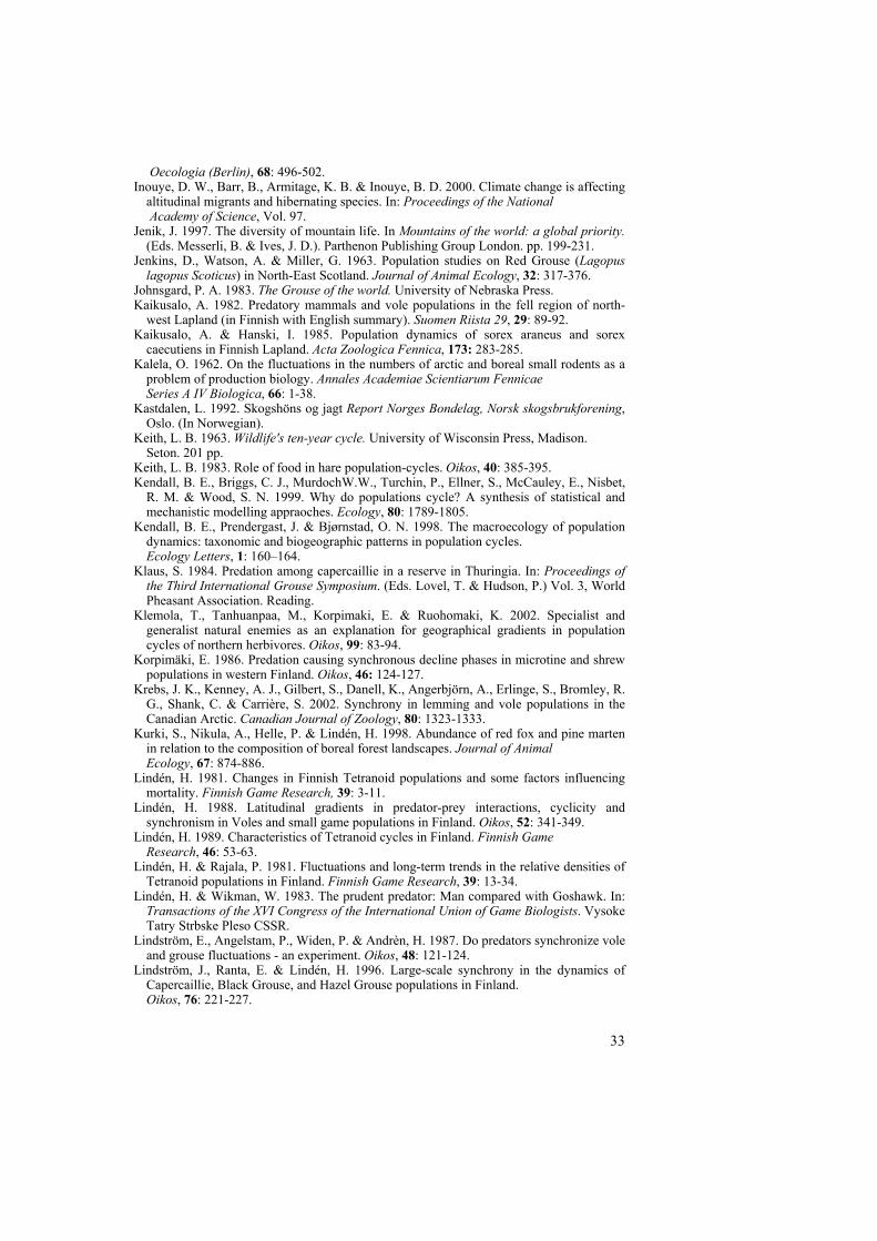
33

Oecologia (Berlin), 68: 496-502. Inouye, D. W., Barr, B., Armitage, K. B. & Inouye, B. D. 2000. Climate change is affecting

altitudinal migrants and hibernating species. In: Proceedings of the National Academy of Science, Vol. 97.

Jenik, J. 1997. The diversity of mountain life. In Mountains of the world: a global priority. (Eds. Messerli, B. & Ives, J. D.). Parthenon Publishing Group London. pp. 199-231.

Jenkins, D., Watson, A. & Miller, G. 1963. Population studies on Red Grouse (Lagopus lagopus Scoticus) in North-East Scotland. Journal of Animal Ecology, 32: 317-376.

Johnsgard, P. A. 1983. The Grouse of the world. University of Nebraska Press. Kaikusalo, A. 1982. Predatory mammals and vole populations in the fell region of north-

west Lapland (in Finnish with English summary). Suomen Riista 29, 29: 89-92. Kaikusalo, A. & Hanski, I. 1985. Population dynamics of sorex araneus and sorex

caecutiens in Finnish Lapland. Acta Zoologica Fennica, 173: 283-285. Kalela, O. 1962. On the fluctuations in the numbers of arctic and boreal small rodents as a

problem of production biology. Annales Academiae Scientiarum Fennicae Series A IV Biologica, 66: 1-38. Kastdalen, L. 1992. Skogshöns og jagt Report Norges Bondelag, Norsk skogsbrukforening,

Oslo. (In Norwegian). Keith, L. B. 1963. Wildlife's ten-year cycle. University of Wisconsin Press, Madison.

Seton. 201 pp. Keith, L. B. 1983. Role of food in hare population-cycles. Oikos, 40: 385-395. Kendall, B. E., Briggs, C. J., MurdochW.W., Turchin, P., Ellner, S., McCauley, E., Nisbet,

R. M. & Wood, S. N. 1999. Why do populations cycle? A synthesis of statistical and mechanistic modelling appraoches. Ecology, 80: 1789-1805.

Kendall, B. E., Prendergast, J. & Bjørnstad, O. N. 1998. The macroecology of population dynamics: taxonomic and biogeographic patterns in population cycles. Ecology Letters, 1: 160–164.

Klaus, S. 1984. Predation among capercaillie in a reserve in Thuringia. In: Proceedings of the Third International Grouse Symposium. (Eds. Lovel, T. & Hudson, P.) Vol. 3, World Pheasant Association. Reading.

Klemola, T., Tanhuanpaa, M., Korpimaki, E. & Ruohomaki, K. 2002. Specialist and generalist natural enemies as an explanation for geographical gradients in population cycles of northern herbivores. Oikos, 99: 83-94.

Korpimäki, E. 1986. Predation causing synchronous decline phases in microtine and shrew populations in western Finland. Oikos, 46: 124-127.

Krebs, J. K., Kenney, A. J., Gilbert, S., Danell, K., Angerbjörn, A., Erlinge, S., Bromley, R. G., Shank, C. & Carrière, S. 2002. Synchrony in lemming and vole populations in the Canadian Arctic. Canadian Journal of Zoology, 80: 1323-1333.

Kurki, S., Nikula, A., Helle, P. & Lindén, H. 1998. Abundance of red fox and pine marten in relation to the composition of boreal forest landscapes. Journal of Animal Ecology, 67: 874-886.

Lindén, H. 1981. Changes in Finnish Tetranoid populations and some factors influencing mortality. Finnish Game Research, 39: 3-11.

Lindén, H. 1988. Latitudinal gradients in predator-prey interactions, cyclicity and synchronism in Voles and small game populations in Finland. Oikos, 52: 341-349.

Lindén, H. 1989. Characteristics of Tetranoid cycles in Finland. Finnish Game Research, 46: 53-63.

Lindén, H. & Rajala, P. 1981. Fluctuations and long-term trends in the relative densities of Tetranoid populations in Finland. Finnish Game Research, 39: 13-34.

Lindén, H. & Wikman, W. 1983. The prudent predator: Man compared with Goshawk. In: Transactions of the XVI Congress of the International Union of Game Biologists. Vysoke Tatry Strbske Pleso CSSR.

Lindström, E., Angelstam, P., Widen, P. & Andrèn, H. 1987. Do predators synchronize vole and grouse fluctuations - an experiment. Oikos, 48: 121-124.

Lindström, J., Ranta, E. & Lindén, H. 1996. Large-scale synchrony in the dynamics of Capercaillie, Black Grouse, and Hazel Grouse populations in Finland. Oikos, 76: 221-227.

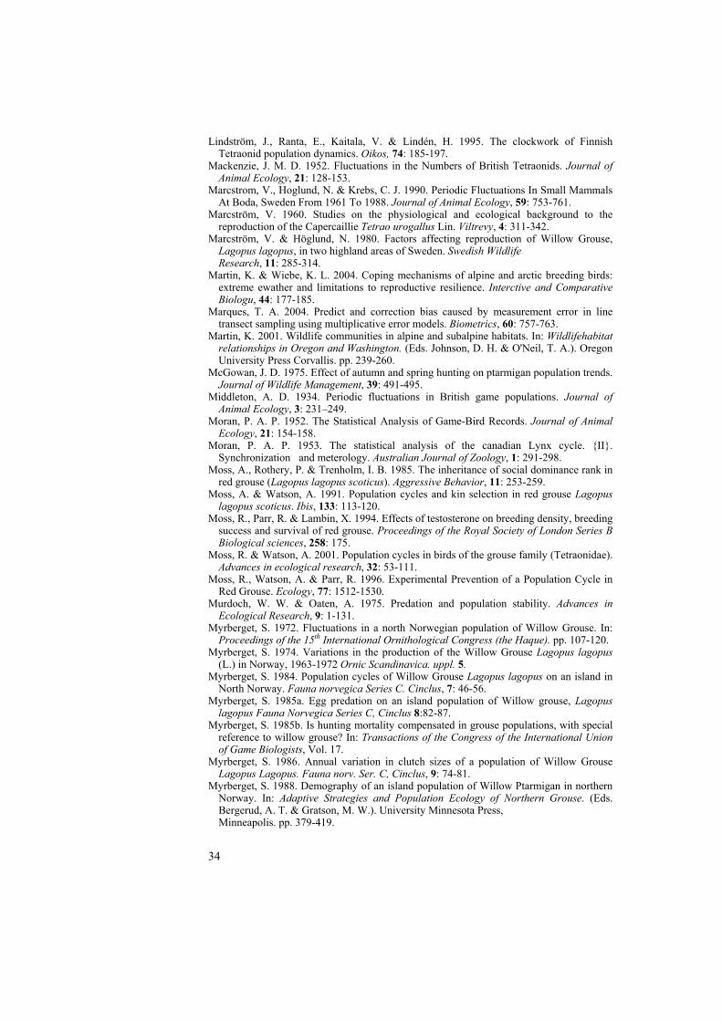
34

Lindström, J., Ranta, E., Kaitala, V. & Lindén, H. 1995. The clockwork of Finnish Tetraonid population dynamics. Oikos, 74: 185-197.

Mackenzie, J. M. D. 1952. Fluctuations in the Numbers of British Tetraonids. Journal of Animal Ecology, 21: 128-153.

Marcstrom, V., Hoglund, N. & Krebs, C. J. 1990. Periodic Fluctuations In Small Mammals At Boda, Sweden From 1961 To 1988. Journal of Animal Ecology, 59: 753-761.

Marcström, V. 1960. Studies on the physiological and ecological background to the reproduction of the Capercaillie Tetrao urogallus Lin. Viltrevy, 4: 311-342.

Marcström, V. & Höglund, N. 1980. Factors affecting reproduction of Willow Grouse, Lagopus lagopus, in two highland areas of Sweden. Swedish Wildlife Research, 11: 285-314.

Martin, K. & Wiebe, K. L. 2004. Coping mechanisms of alpine and arctic breeding birds: extreme ewather and limitations to reproductive resilience. Interctive and Comparative Biologu, 44: 177-185.

Marques, T. A. 2004. Predict and correction bias caused by measurement error in line transect sampling using multiplicative error models. Biometrics, 60: 757-763.

Martin, K. 2001. Wildlife communities in alpine and subalpine habitats. In: Wildlifehabitat relationships in Oregon and Washington. (Eds. Johnson, D. H. & O'Neil, T. A.). Oregon University Press Corvallis. pp. 239-260.

McGowan, J. D. 1975. Effect of autumn and spring hunting on ptarmigan population trends. Journal of Wildlife Management, 39: 491-495.

Middleton, A. D. 1934. Periodic fluctuations in British game populations. Journal of Animal Ecology, 3: 231–249.

Moran, P. A. P. 1952. The Statistical Analysis of Game-Bird Records. Journal of Animal Ecology, 21: 154-158.

Moran, P. A. P. 1953. The statistical analysis of the canadian Lynx cycle. {II}. Synchronization and meterology. Australian Journal of Zoology, 1: 291-298.

Moss, A., Rothery, P. & Trenholm, I. B. 1985. The inheritance of social dominance rank in red grouse (Lagopus lagopus scoticus). Aggressive Behavior, 11: 253-259.

Moss, A. & Watson, A. 1991. Population cycles and kin selection in red grouse Lagopus lagopus scoticus. Ibis, 133: 113-120.

Moss, R., Parr, R. & Lambin, X. 1994. Effects of testosterone on breeding density, breeding success and survival of red grouse. Proceedings of the Royal Society of London Series B Biological sciences, 258: 175.

Moss, R. & Watson, A. 2001. Population cycles in birds of the grouse family (Tetraonidae). Advances in ecological research, 32: 53-111.

Moss, R., Watson, A. & Parr, R. 1996. Experimental Prevention of a Population Cycle in Red Grouse. Ecology, 77: 1512-1530.

Murdoch, W. W. & Oaten, A. 1975. Predation and population stability. Advances in Ecological Research, 9: 1-131.

Myrberget, S. 1972. Fluctuations in a north Norwegian population of Willow Grouse. In: Proceedings of the 15th International Ornithological Congress (the Haque). pp. 107-120.

Myrberget, S. 1974. Variations in the production of the Willow Grouse Lagopus lagopus (L.) in Norway, 1963-1972 Ornic Scandinavica. uppl. 5.

Myrberget, S. 1984. Population cycles of Willow Grouse Lagopus lagopus on an island in North Norway. Fauna norvegica Series C. Cinclus, 7: 46-56.

Myrberget, S. 1985a. Egg predation on an island population of Willow grouse, Lagopus lagopus Fauna Norvegica Series C, Cinclus 8:82-87.

Myrberget, S. 1985b. Is hunting mortality compensated in grouse populations, with special reference to willow grouse? In: Transactions of the Congress of the International Union of Game Biologists, Vol. 17.

Myrberget, S. 1986. Annual variation in clutch sizes of a population of Willow Grouse Lagopus Lagopus. Fauna norv. Ser. C, Cinclus, 9: 74-81.

Myrberget, S. 1988. Demography of an island population of Willow Ptarmigan in northern Norway. In: Adaptive Strategies and Population Ecology of Northern Grouse. (Eds. Bergerud, A. T. & Gratson, M. W.). University Minnesota Press, Minneapolis. pp. 379-419.

35

Myrberget, S. 1989. Norwegian research on willow grouse: implications for management. Finnish Game Research, 46: 17-25.

Myrberget, S. & Lund-Tangen, H. I. 1990. Cyclic variations in small game populations in central Norway. In: Transactions of the 19th International Union of Game Biologists Congress, Norwegian Institute for Nature Research. Trondhiem, NINA.

Palmer, W. L. 1956. Ruffed grouse population studies on hunted and unhunted areas. In: Twenty-first North American Wildlife Conference, Vol. 21.

Palmer, W. L. & Bennett, C. L. J. 1963. Relation of season length to hunting harvest of ruffed grouse. Journal of Wildlife Management, 27: 634-639.

Parker, H. 1984. Effect of corvid removal on reproduction of willow ptarmigan and black grouse. Journal of Wildlife Management, 48: 1197-1205.

Pedersen, H. C., Steen, H., Kastdalen, L., Svendsen, W. & Brösteh, H. 1999. Betydningen av jakt på lirypebestander. Framdriftsrapport 1996-1998, (in Norwegian with English summary). NINA Oppdragsmelding.

Post, E. & Stenseth, N. C. 1999. Climatic variability, plant phenology, and northern ungulates. Ecology, 80: 1322–1339.

Post, J. R., Sullivan, M., Cox, S., Lester, N. P., Walters, C. J., Parkinson, E. A., Paul, A. J., Jackson, L. & Shuter, B. J. 2002. Canada’s Recreational Fisheries: The Invisible Collapse? Fisheries, 27: 6-17.

Potapov, R. L. & Flint, V. E. 1989. Handbuch der Vögel der Sowjetunion. Band 4 Galliformes, Gruiformes. Ziemsen Verlag Wittenberg. Lutherstadt, Germany.

Potts, G. R., Tapper, S. C. & Hudson, P. J. 1984. Population fluctuations in Red Grouse: Analysis of bag records and a simulation model. Journal of Animal Ecology, 35: 21-36.

Ranta, E., Lindström, J., Kaitala, V., Kokko, H., Linden, H. & Helle, E. 1997. Solar activity and Hare dynamics: a cross continental comparison. American Naturalist, 149: 765-775.

Roland, J., Keyghobadi, N. & Fownes, S. 2000. Alpine Parnassius butterfly dispersal: effects of landscape and population size. Ecology, 81: 1642-1653.

Royama, T. 1984. Population dynamics of the spruce budworm Choristoneura fumiferana. Ecological Monographs, 54: 429–462.

Royama, T. 1992. Analytichal population dynamics. Chapman & Hall. London.371 pp. Rörvik, K.-A., Pedersen, H. C. & Steen, J. B. 1998. Dispersal in willow ptarmigan Lagopus

lagopus - who is dispersing and why? 4: 91-96. Sæther, B.-E., Engen, S., Lande, R., Arcese, P. & Smith, J. N. M. 2000. Estimating the time

to extinction in an island population of song sparrows. In: Proceedings of the Royal Society of London, Series B, 267: 621–626.

Saether, B.-E., Engen, S. & Matthysen, E. 2002. Demographic Characteristics and Population Dynamical Patterns of Solitary Birds. Science, 295: 2070-2073.

Saether, B. E., Engen, S., Moller, A. P., Matthysen, E., Adriaensen, F., Fiedler, W., Leivits, A., Lambrechts, M. M., Visser, M. E., Anker-Nilssen, T., Both, C., Dhondt, A. A., McCleery, R. H., McMeeking, J., Potti, J., Rostad, O. W. & Thomson, D. 2003. Climate variation and regional gradients in population dynamics of two hole-nesting passerines. Proceedings of the Royal Society Series B, 270: 2397-2404.

Samuel, M. D. & Fuller, M. R. 1994. Wildlife radiotelemetry. In: Research and management techniques for wildlife and habitats. (Eds. Bookhout, T. A.). The Wildlife Sot., Bethesda, Maryland. pp 370-418.

Siivonen, L. 1948. Structure of short cyclic fluctuation in numbers of mammals and birds in the northern parts of the northern hemisphere. Papers in Game Research, 1: 1-166.

Small, R. J., Marcström, V. & Willebrand, T. 1993. Synchronous and nonsynchronous population fluctuations of some predators and their prey in Central Sweden. Ecography, Copenhagen., 16: 360-364.

Smith, A. A. 1997. Movement, dispersal and survival patterns of Swedish willow grouse (Lagopus lagopus L.) Edward Grey Institute, Department of Zoology.

University of Oxford, Oxford. Smith, A. A. & Willebrand, T. 1999. Mortality causes and survival rates of hunted and

unhunted Willow Grouse. Journal of Wildlife Management, 63: 722-730. Sonnerud, G. A. 1988. What causes extended lows in microtine cycles? Analysis of

fluctuations in sympatric shrews and microtine populations in Fennoscandia.

36

Oecologia, 76: 37-42. Steen, H. & Erikstad, K. E. 1996. Sensitivity of Willow Grouse Lagopus lagopus

population dynamics to variations in demographic parameters. Wildlife Biology, 2: 27-35. Steen, J. B., Andersen, Ö., Säbö, A., Pedersen, H. C. & Erikstad, K. E. 1988a. Viability of

newly hatched chicks of Willow Ptarmigan Lagopus lagopus. Ornis Scandinavica Copenhagen., 19: 93-96.

Steen, J. B., Steen, H., Stenseth, N. C., Myrberget, S. & Markström, V. 1988b. Microtine density and weather as a predictors of chick production in Willow Ptarmigan, Lagopus lagopus. Oikos 51: 367-376.

Stenseth, N. C., Falck, W., Chan, K.-S., Bjornstad, O. N., O´Donoghue, M., Tong, H., Boonstra, R., Boutin, S., Krebs, C. H. & Yoccoz, N. G. 1998. From patterns to processes: Phase and density dependencies in the Canadian lynx cycle. Ecology, 95: 15430-15435.

Taylor, A. D. 1990. Metapopulations, dispersal, and predator-prey dynamics: and overview. Ecology, 71: 429-433.

Thomas, L., Burnham, K. P. & Buckland, S. T. 2004. Temporal inferences from distance sampling surveys. In: Advanced Distance Sampling. (Eds. Buckland, S. T., Anderson, D.R., Burnham, K.P., Laake, J.L., Borchers, D.L., & Thomas, L.). Oxford University Press, Oxford. pp. 71-107.

Thomas, L., Laake, J. L., Strindberg, S., Marques, F. F. C., Buckland, S. T., Borchers, D. L., Anderson, D. R., Burnham, K. P., Hedley, S. L., Pollard, J. H. & Bishop, J. R. B. 2003. Distance 4.1 Release 2, St. Anderws: Research Unit for Wildlife Population Assessment, University of St .Andrews.

Tornberg, R. & Sulkava, S. 1991. The effect of changing tetraonid populations on the nutrition and breeding success of the goshawk (Accipiter gentilis L.) in Northern Finland. Aquilo Serie Zoologica, 28: 23–33.

Turchin, P. 2003. Complex Population Dynamics: A Theoretical/Empirical Synthesis. Princeton University Press.

Turchin, P. & Hanski, I. 1997. An empirically based model for latitudinal gradient in vole population dynamics. American Naturalist, 149: 842-874.

Watson, A. 1965. A population study of ptarmigan (Lagopus mutus) in Scotland. Journal of Animal Ecology, 34: 135-172.

Watson, A., Moss, A., Rothery, P. & Parr, R. 1984. Demographic causes and predictive models of population fluctuations in red grouse. Journal of Animal Ecology, 53: 639-662.

Watson, A. & Moss, R. 1979. Populations cycles in Tetraonidae Ornis Fennica 57:87-109. Watson, A., Moss, R. & Rae, S. R. 1998. Population dynamics of Scottish rock ptarmigan

cycles. Ecology, 79: 1174-1192. Weeden, R. B. & Theberge, J. B. 1972. The dynamic of a fluctuating population of rock

ptarmigan in Alaska. In: Proceedings of the International Ornithological Congress, 15: 90-106.

Willebrand, T. 1996. Ripan och småviltjakten på statens mark ovanför odlingsgränsen och på renbetesfjällen. 3.18 Jordbruksverket, Naturvårdsverket och Sametinget. Utvärderingen av småviltjakten och handredskapsfisket ovan odlingsgränsen och på renbetesfjällen. NV, Stockholm. Stockholm: Naturvårdsverket (Swedish Environmental Protection Agency). (In Swedish).

Williams, C. K., Ives, A. R., Applegate, R. D. & Ripa, J. 2004. The collapse of cycles in the dynamics of North American grouse populations. Ecology Letters, 7: 1135-1142.

Williams, D. W. & Liebhold, A. 2000. Spatial synchrony of spruce budworm outbreaks in eastern North America. Ecology, 81: 2753–2766.

Williams, G. R. 1954. Population fluctuations in some northern hemisphere game birds (Tetraonidae). Journal of Animal Ecology, 23: 1-34.

Williams, J. 1985. Statistical analysis of fluctuations in red grouse bag data. Oecologia, 65: 269-272.