TEMPLATE ELASTIC-PLASTIC COMPUTATIONS IN...

CREPORT NO. UCD/CGM-01/02

TC

B BZ

DCU S

ENTER FOR GEOTECHNICAL MODELING

EMPLATE ELASTIC-PLASTIC OMPUTATIONS IN GEOMECHANICS

Y

. JEREMIC . YANG

EPARTMENT OF CIVIL & ENVIRONMENTAL ENGINEERING OLLEGE OF ENGINEERING NIVERSITY OF CALIFORNIA AT DAVIS

EPTEMBER 2001

Bor

is J

erem

ic: D

raft

Pap

erINTERNATIONAL JOURNAL FOR NUMERICAL AND ANALYTICAL METHODS IN GEOMECHANICS

Int. J. Numer. Anal. Meth. Geomech. 2001; 01:1{6 Prepared using nagauth.cls [Version: 2000/03/22 v1.0]

Template Elastic{Plastic Computations in Geomechanics

Boris Jeremi�c�and Zhaohui Yang

Department of Civil and Environmental Engineering, University of California,

Davis, CA 95616

submitted for publication in the International Journal for Numerical and Analytical Methods

in Geomechanics, July 2001.

SUMMARY

In this paper we present a new approach to computations in elasto{plastic geomechanics. The

approach is based on the object oriented design philosophy and observations on similarity of most

incremental elastic{plastic material models. This new approach to elastic{plastic computations in

geomechanics allows for creation of template material models. The analysis of template material

models will in turn allow for an easy implementation of other elastic{plastic material models based on

the object oriented design principles. Furthermore we present some illustrative implementation details.

Finally we present analysis results that emphasize features of template elastic{plastic computations

in geomechanics.

Copyright c 2001 John Wiley & Sons, Ltd.

�Correspondence to: Boris Jeremi�c, Department of Civil and Environmental Engineering, University of

California, One Shields Ave., Davis, CA 95616, [email protected]

Contract/grant sponsor: NSF; contract/grant number: EEC-9701568

Copyright c 2001 John Wiley & Sons, Ltd.

Bor

is J

erem

ic: D

raft

Pap

er2 BORIS JEREMI�C AND ZHAOHUI YANG

key words: Elasto{plastic geomechanics; template constitutive driver; object oriented design

1. INTRODUCTION

Current approach to the development and implementation of elastic{plastic material models in

computational geomechanics relies heavily on a �nite number of existing yield functions, ow

potential rules and evolution laws. The yield function de�nitions are usually based on a set of

already existing shapes. We mention a few of the most prominent examples of yield functions:

von Mises , Drucker{Prager, Mohr{Coulomb, Cam{Clay (Roscoe et al. [39], Scho�eld and

Wroth [40], Roscoe et al. [38] and Roscoe and Burland [37]), Parabolic model (Menetrey and

Willam [31]) and Lade's yield functions (Lade [21, 24]).

In addition to that, plastic ow direction is in most cases de�ned as normal to the potential

surface, which is usually quite similar to the yield surface (function). There are some exceptions

in which the plastic ow direction is directly de�ned in stress space. Nevertheless all of the

de�ned yield surfaces can be used, with small changes, as plastic potential surfaces.

The hardening and/or softening behavior of the material model is controlled by the evolution

laws. These laws provide functional relationship between the internal variable and the size and

shape of yield surface and plastic ow directions (or potential surface)

It is important to note that a large majority of incremental elastic{plastic material models

developed for geomechanics consist of the three main elements: (a) the yield functions

(surfaces); (b) the plastic ow direction (directly or through the potential function); and

(c) the evolution hardening{softening rules (functions describing the evolutions of the yield

function and plastic ow directions with the inelastic deformations). This observation has

Copyright c 2001 John Wiley & Sons, Ltd. Int. J. Numer. Anal. Meth. Geomech. 2001; 01:1{6

Prepared using nagauth.cls

Bor

is J

erem

ic: D

raft

Pap

erTEMPLATE ELASTIC{PLASTIC COMPUTATIONS IN GEOMECHANICS 3

practical consequence in that it is possible to unify the implementation of the incremental

elastic{plastic equations under a single framework. This paper describes the theoretical basis

and the implementation details for the template elastic{plastic computations in geomechanics.

The object oriented philosophy has been extensively used in computational mechanics

recently. To this end we mention early experimental developments and implementations of

Donescu and Laursen [6], Zimmermann et al. [48, 7, 47, 10], Forde et al. [14], Miller [32],

Pidaparti and Hudli [36], Scholz [41], Zeglinski et al. [45], Fenves [12], Foerch et al. [13], and

Men�entrey and Zimmermann [30].

While the early works have focused on basic issues in the object oriented design of programs,

they were hindered by the lack of standard for C++, which is most of the time programming

language of choice. Recent acceptance of the standard [1] has provided developers of the

object{oriented �nite element programs based on C++ with a stable platform. More recent

work has focused on designing and implementing large �nite element programs for sequential

and parallel platforms. There was far less work in the general area of object oriented design and

implementation for material non{linear analysis of solids. We mention recent work by Dubois{

P�elerin and Pegon [8], Eyheramendy and Zimmermann [11], and by Jeremi�c and Sture [19].

We also note an excellent bibliography of recent works in object oriented �nite element by

Mackerle [27].

The developments we present in this paper are part of much larger endeavor currently

underway within the Paci�c Earthquake Engineering Research Center and led by Professor

Fenves (Archer et al. [2], Archer [3] and McKenna [29]). This endeavor has recently resulted

in a public release of the OpenSees platform [33] for Open Seismic Earthquake Engineering

Simulations.



Bor

is J

erem

ic: D

raft

Pap


The paper is organized as follows: In section 2 we review common elastic and elastic{

plastic models used in computational geomechanics. Section 3 reviews basic elastic{plastic

formulations. This section also presents two commonly used algorithms for integrating

constitutive equations. In section 4 we present the object{oriented design and implementation.

Section 5 present a number of illustrative elastic{plastic simulations. Finally, section 6 presents

a set of conclusions and future work directions.

2. ELASTIC{PLASTIC MATERIAL MODELS

In this section we present elements of general elastic{plastic material models for geomaterials.

We describe various forms of the yield functions, plastic ow directions and hardening and

softening laws.

2.1. Elasticity

In elasticity the relationship between the stress tensor �ij and the strain tensor �kl can be

represented in the following form:

�ij = � (�ij) (1)

In it's simplest form it reads

�ij = Eijkl�kl (2)

where Eijkl is the fourth order elastic sti�ness tensor with 81 independent components in total.

The elastic sti�ness tensor features both minor symmetry Eijkl = Ejikl = Eijlk and major

symmetry Eijkl = Eklij (e.g. Jeremi�c and Sture [18]). The number of independent components

for such elastic sti�ness tensor is 21 (cf. Spencer [42]).



Bor

is J

erem

ic: D

raft

Pap


Most of the models used to describe elastic behavior of soils assume isotropic behavior.

The most general form of the isotropic elastic sti�ness tensor of rank 4 has the following

representation:

Eijkl = �ÆijÆkl + � (ÆikÆjl + ÆilÆjk) (3)

where � and � are the Lam�e coeÆcients:

� =�E

(1 + �) (1� 2�); � =

E

2 (1 + �)(4)

and E and � are Young's Modulus and Poisson's ratio respectively. Equation (3) can be written

in terms of E and � as:

Eijkl =E

2 (1 + �)

�2�

1� 2�ÆijÆkl + ÆikÆjl + ÆilÆjk

�(5)

The same relation in terms of bulk modulus K and shear modulus G is:

Eijkl = KÆijÆkl +G

��2

3ÆijÆkl + ÆikÆjl + ÆilÆjk

�(6)

where K and G are given as:

K = �+2

3� ; G = � (7)

The elastic isotropic behavior of soils obeys Hooke's law with a constant Poisson's ratio. The

variation of the Young's modulus E is usually assumed to be a function of the stress state. To

this end we use four di�erent elastic laws.

Linear Elastic Model. Linear elastic law is the simplest one and assumes constant Young's

modulus E and constant Poisson's Ration �.



Bor

is J

erem

ic: D

raft

Pap


Non{linear Elastic Model #1. This nonlinear model (cf. Janbu [16], Duncan and Chang

[9]) assumes dependence of the Young's modulus on the minor principal stress �3 = �min in

the form

E = Kpa

��3

pa

�n

(8)

Here, pa is the atmospheric pressure in the same units as E and stress. The two material

constants K and n are constant for a given void ratio.

Non{linear Elastic Model #2. If Young's modulus and Poisson's ratio are replaced by

the shear modulus G and bulk modulus K the non{linear elastic relationship can be expressed

in terms of the normal e�ective mean stress p as

G and/or K = AF (e;OCR)pn (9)

where e is the void ratio, OCR is the overconsolidation ratio and p = �ii=3 is the mean e�ective

stress (Hardin [15]).

Lade's Non{linear Elastic Model. Lade and Nelson [25] and Lade [23] proposed a

nonlinear elastic model based on Hooke's law in which Poisson ratio � is kept constant.

According to this model, Young's modulus can be expressed in terms of a power law as:

E =M pa

�I1

pa

�2+

�61 + �

1� 2�

�J2D

p2a

!�

(10)

where I1 = �ii is the �rst invariant of the stress tensor and J2D = (sijsij)=2 is the second

invariant of the deviatoric stress tensor sij = �ij ��kkÆij=3. The parameter pa is atmospheric

pressure expressed in the same unit as E, I1 andpJ2D and the modulus number M and the

exponent � are constant, dimensionless numbers.



Bor

is J

erem

ic: D

raft

Pap


2.2. Yield Functions

The typical plastic behavior of frictional materials is in uenced by both normal and shear

stresses. It is usually assumed that there exists a yield surface F in the stress space that

encompasses the elastic region. States of stress inside the yield surface are assumed to be elastic

(linear or nonlinear). Stress states on the surface are assumed to produce plastic deformations.

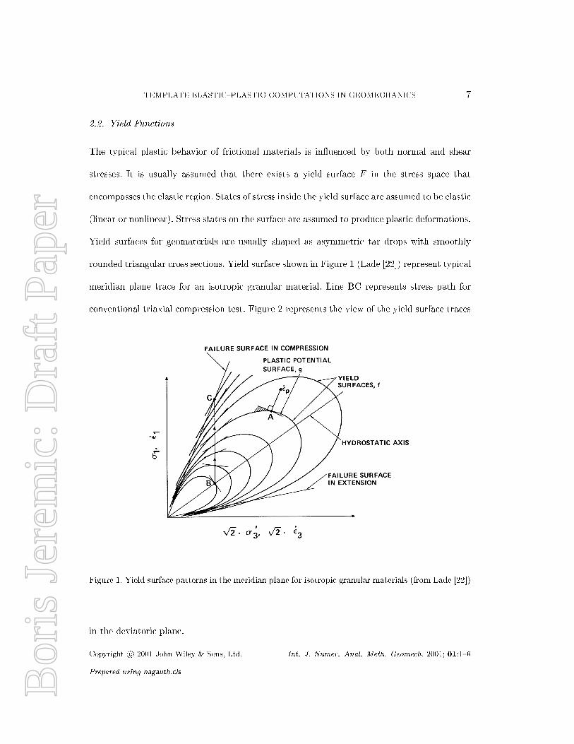
Yield surfaces for geomaterials are usually shaped as asymmetric tar drops with smoothly

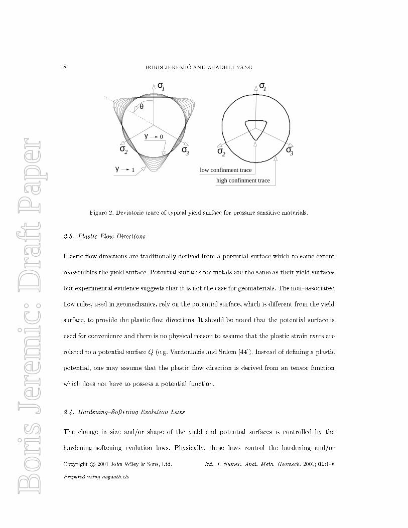
rounded triangular cross sections. Yield surface shown in Figure 1 (Lade [22]) represent typical

meridian plane trace for an isotropic granular material. Line BC represents stress path for

conventional triaxial compression test. Figure 2 represents the view of the yield surface traces

Figure 1. Yield surface patterns in the meridian plane for isotropic granular materials (from Lade [22])

in the deviatoric plane.



Bor

is J

erem

ic: D

raft

Pap


σ2 σ3

σ1

γ 1

γ 0

σ3σ2

σ1

θ

low confinment trace

high confinment trace

Figure 2. Deviatoric trace of typical yield surface for pressure sensitive materials.

2.3. Plastic Flow Directions

Plastic ow directions are traditionally derived from a potential surface which to some extent

reassembles the yield surface. Potential surfaces for metals are the same as their yield surfaces

but experimental evidence suggests that it is not the case for geomaterials. The non{associated

ow rules, used in geomechanics, rely on the potential surface, which is di�erent from the yield

surface, to provide the plastic ow directions. It should be noted that the potential surface is

used for convenience and there is no physical reason to assume that the plastic strain rates are

related to a potential surface Q (e.g. Vardoulakis and Sulem [44]). Instead of de�ning a plastic

potential, one may assume that the plastic ow direction is derived from an tensor function

which does not have to possess a potential function.

2.4. Hardening{Softening Evolution Laws

The change in size and/or shape of the yield and potential surfaces is controlled by the

hardening{softening evolution laws. Physically, these laws control the hardening and/or



Bor

is J

erem

ic: D

raft

Pap


softening process during loading. Depending on the evolution type they control, these laws can

be in general separated into isotropic and kinematic (also called anisotropic). The isotropic

evolution laws control the size of the yield surface through a single scalar variable. This is

usually related to the Coulomb friction or to the mean stress values at isotropic yielding. The

non{isotropic evolution laws can be further specialized to rotational, translational kinematic

and distortional. It should be noted that all of the kinematic evolution laws can be treated as

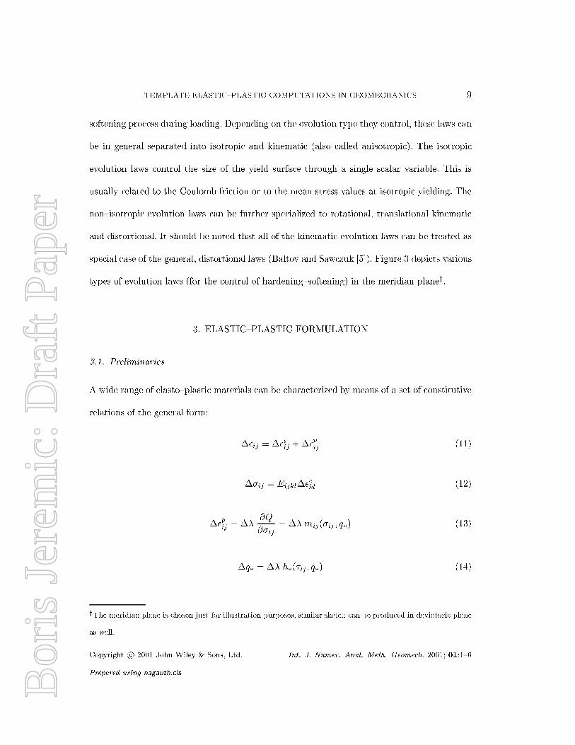
special case of the general, distortional laws (Baltov and Sawczuk [5]). Figure 3 depicts various

types of evolution laws (for the control of hardening{softening) in the meridian planey.

3. ELASTIC{PLASTIC FORMULATION

3.1. Preliminaries

A wide range of elasto{plastic materials can be characterized by means of a set of constitutive

relations of the general form:

��ij = ��eij +��pij (11)

��ij = Eijkl��ekl (12)

��pij = ��@Q

@�ij= �� mij(�ij ; q�) (13)

�q� = �� h�(�ij ; q�) (14)

yThe meridian plane is chosen just for illustration purposes, similar sketch can be produced in deviatoric plane

as well.



Bor

is J

erem

ic: D

raft

Pap


q

p

q

ppc

q

p

q

p

a) b)

d)c)

Figure 3. Various types of evolution laws that control hardening and/or softening of elastic{

plastic material models: (a) Isotropic (scalar) controlling equivalent friction angle and

isotropic yield stress. (b) Rotational kinematic hardening (second order tensor) controlling

pivoting around �xed point (usually stress origin) of the yield surface. (c) Translational

kinematic hardening (second order tensor) controlling translation of the yield surface. (d)

Distortional (fourth order tensor) controlling the shape of the yield surface.

where, following standard notation ��ij ; ��eij and ��pij denotes the increment in total, elastic

and plastic strain tensor, ��ij is the increment in Cauchy stress tensor, and �q� signi�es

increments in some suitable set of internal variables z. The asterisk in the place of indices in

q� replaces n indicesx. Equation (11) expresses the commonly assumed additive decomposition

of the in�nitesimal strain tensor into elastic and plastic parts. Equation (12) represents the

zIn the simplest models of plasticity the internal variables are taken as either incremental plastic strain

components ��p

ijor the hardening variables � de�ned, for example as a function of inelastic (plastic) work, i.e.

� = f (W p). See Lubliner [26], page 115.

xfor example ij if the variable is �p

ij, or nothing if the variable is a scalar value, i.e. � .



Bor

is J

erem

ic: D

raft

Pap


generalized Hooke's law which linearly relates stresses and elastic strains through a sti�ness

modulus tensorEijkl . Equation (13) expresses a generally associated or non-associated ow rule

for the incremental plastic strain and (14) describes a suitable set of hardening/softening laws,

which govern the evolution of the plastic variables. In these equations, mij is the plastic ow

direction, h� the plastic moduli and �� is a plastic (consistency) parameter to be determined

with the aid of the loading{unloading criterion, which can be expressed in terms of the Karush{

Kuhn{Tucker ([20]) conditions as:

F (�ij ; q�) � 0 (15)

�� 0 (16)

F �� = 0 (17)

In the previous equations F (�ij ; q�) denotes the yield function of the material and (15)

characterizes the corresponding elastic domain, which is presumably convex. Along any process

of loading, conditions (15), (16) and (17) must hold simultaneously. For F < 0, equation (17)

yields �� = 0, i.e. elastic behavior, while plastic ow is characterized by �� > 0, which with

(17) is possible only if the yield criterion is satis�ed, i.e. F = 0. From the latter constraint, in

the process of plastic loading the plastic consistency conditions is obtained in the form:

dF =@F

@�ijd�ij +

@F

@q�dq� = nijd�ij + ��dq� = 0 (18)

where :

nij =@F

@�ij(19)

�� =@F

@q�(20)



Bor

is J

erem

ic: D

raft

Pap


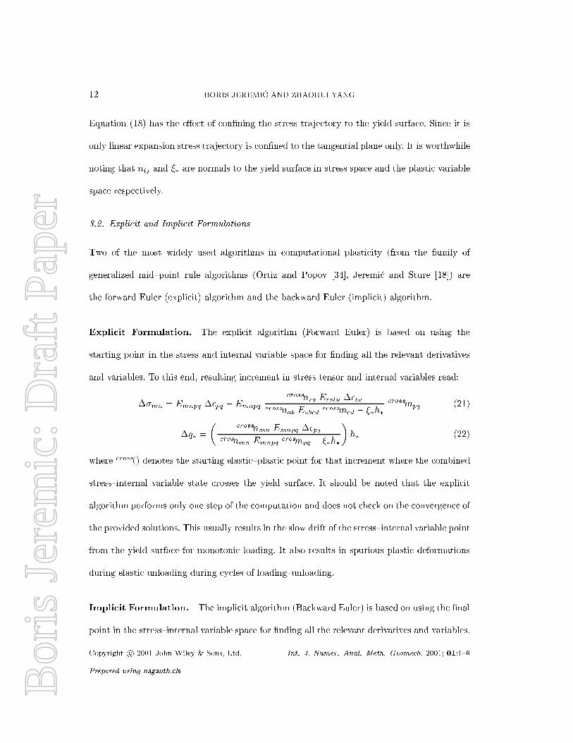
Equation (18) has the e�ect of con�ning the stress trajectory to the yield surface. Since it is

only linear expansion stress trajectory is con�ned to the tangential plane only. It is worthwhile

noting that nij and �� are normals to the yield surface in stress space and the plastic variable

space respectively.

3.2. Explicit and Implicit Formulations

Two of the most widely used algorithms in computational plasticity (from the family of

generalized mid{point rule algorithms (Ortiz and Popov [34], Jeremi�c and Sture [18]) are

the forward Euler (explicit) algorithm and the backward Euler (implicit) algorithm.

Explicit Formulation. The explicit algorithm (Forward Euler) is based on using the

starting point in the stress and internal variable space for �nding all the relevant derivatives

and variables. To this end, resulting increment in stress tensor and internal variables read:

��mn = Emnpq ��pq �Emnpq

crossnrs Erstu ��tucrossnab Eabcd

crossmcd � ��h�

crossmpq (21)

�q� =

�crossnmn Emnpq ��pq

crosnmn Emnpqcrosmpq � ��h�

�h� (22)

where cross() denotes the starting elastic{plastic point for that increment where the combined

stress{internal variable state crosses the yield surface. It should be noted that the explicit

algorithm performs only one step of the computation and does not check on the convergence of

the provided solutions. This usually results in the slow drift of the stress{internal variable point

from the yield surface for monotonic loading. It also results in spurious plastic deformations

during elastic unloading during cycles of loading{unloading.

Implicit Formulation. The implicit algorithm (Backward Euler) is based on using the �nal

point in the stress{internal variable space for �nding all the relevant derivatives and variables.



Bor

is J

erem

ic: D

raft

Pap


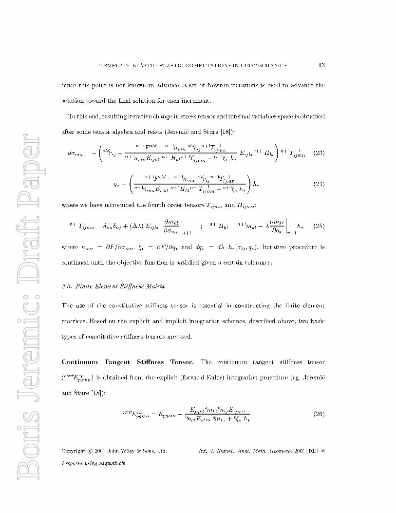
Since this point is not known in advance, a set of Newton iterations is used to advance the

solution toward the �nal solution for each increment.

To this end, resulting iterative change in stress tensor and internal variables space is obtained

after some tensor algebra and reads (Jeremi�c and Sture [18]):

d�mn = �

oldrij +

n+1F old � n+1nmnoldrij

n+1T�1ijmn

n+1nmnEijkln+1Hkl

n+1T�1ijmn �

n+1�� h�Eijkl

n+1Hkl

!n+1T�1

ijmn (23)

q� =

n+1F old � n+1nmn

oldrijn+1T�1

ijmn

n+1nmnEijkln+1Hkl

n+1T�1ijmn �

n+1�� h�

!h� (24)

where we have introduced the fourth order tensors Tijmn and Hijmn:

n+1Tijmn = ÆimÆnj + (.��) Eijkl@mkl

@�mn

��n+1

; n+1Hkl =n+1mkl + �

@mkl

@q�

��n+1

h� (25)

where nmn = @F=@�mn, �� = @F=@q� and dq� = d� h�(�ij ; q�). Iterative procedure is

continued until the objective function is satis�ed given a certain tolerance.

3.3. Finite Element Sti�ness Matrix

The use of the constitutive sti�ness tensor is essential in constructing the �nite element

matrices. Based on the explicit and implicit integration schemes, described above, two basic

types of constitutive sti�ness tensors are used.

Continuum Tangent Sti�ness Tensor. The continuum tangent sti�ness tensor

(contEeppqmn) is obtained from the explicit (forward Euler) integration procedure (eg. Jeremi�c

and Sture [18]):

contEeppqmn = Epqmn �

Epqklnmkl

nnijEijmn

nnotEotrsnmrs + n�� h�

(26)



Bor

is J

erem

ic: D

raft

Pap


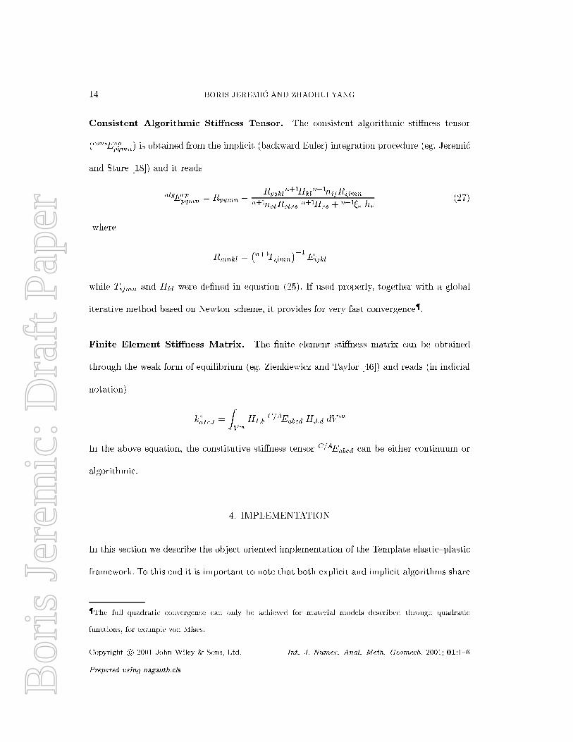
Consistent Algorithmic Sti�ness Tensor. The consistent algorithmic sti�ness tensor

(consEeppqmn) is obtained from the implicit (backward Euler) integration procedure (eg. Jeremi�c

and Sture [18]) and it reads

algEeppqmn = Rpqmn �

Rpqkln+1Hkl

n+1nijRijmn

n+1notRotrsn+1Hrs + n+1�� h�

(27)

where

Rmnkl =�n+1Tijmn

��1Eijkl

while Tijmn and Hkl were de�ned in equation (25). If used properly, together with a global

iterative method based on Newton scheme, it provides for very fast convergence{.

Finite Element Sti�ness Matrix. The �nite element sti�ness matrix can be obtained

through the weak form of equilibrium (eg. Zienkiewicz and Taylor [46]) and reads (in indicial

notation)

keaIcJ =

ZVm

HI;bC=AEabcd HJ;d dV

m

In the above equation, the constitutive sti�ness tensor C=AEabcd can be either continuum or

algorithmic.

4. IMPLEMENTATION

In this section we describe the object oriented implementation of the Template elastic{plastic

framework. To this end it is important to note that both explicit and implicit algorithms share

{The full quadratic convergence can only be achieved for material models described through quadratic

functions, for example von Mises.



Bor

is J

erem

ic: D

raft

Pap


common set of material functions and their derivatives with respect to the stress or internal

variable tensors. For example the �rst derivatives of the yield function nij = @F=@�ij appears

in both explicit and implicit integration algorithms and can be implemented in general form

without specifying particular material model to be used.

Our implementation relies on three classes:

� MatPoint

� EPState

� Template3Dep

4.1. The MatPoint Class

The MatPoint class represents the spatial setting of the material point in the solid. It also

includes the objects of NDMaterial type. The NDMaterial objects represent a container for all

the material models in the OpenSees framework.

4.2. The EPState Class

The EPState class contains the elastic{plastic state of the material point. This class is designed

to be as general as possible. The data part of the class includes current, incremental, iterative

and committed stress and strain tensors, current and committed constitutive sti�ness tensor,

and an array of initial, current and committed scalar and tensorial internal variables. The

EPState class can be easily expanded to accommodate new developments. It should be noted

that the type of constitutive sti�ness tensor is a function of the constitutive integration method

used. For the explicit algorithm continuum tangent sti�ness tensor is used while for the implicit

algorithm, consistent tangent sti�ness tensor is used.



Bor

is J

erem

ic: D

raft

Pap


4.3. The Template3Dep Class

The Template3Dep class represents the container class for yield surfaces, ow directions and

evolution laws described in sections 2.2, 2.3 and 2.4 respectively. This class allows for di�erent

yield criteria, ow directions and evolution laws to be synthesized into a working elastic{plastic

material model. The Template3Dep class inherits all the functionality from the NDMaterial

class. The NDMaterial class is an abstract class. It provides the interface that should be

followed when introducing new NDMaterial subclasses. More on NDMaterial class can be found

at the OpenSees web repository [33]. The Template3Dep class features a number of constructors

which are used to combine di�erent yield surface, plastic potential surface and evolution

laws. This class features two methods for integration of the constitutive equations, namely

ForwardEulerEPState and BackwardEulerEPState. Both methods can also be used with the

subincrementation technique in which user supplies number of subincrements to be used for

desired convergence. Both the explicit (ForwardEulerEPState) and the implicit algorithm

(BackwardEulerEPState) as well as their subincrementation counterparts, return an EPState

object. Moreover, each of the integration algorithms will also create corresponding tangent

constitutive tensor. That is, the ForwardEulerEPState method will create a continuum

tangent sti�ness tensor while the BackwardEulerEPState will create a consistent tangent

sti�ness tensor.

In addition to the above three classes, the implementation relies on a number of yield

functions, plastic potential functions and evolution laws. The implementation for each is

provided in a separate �le and includes a number of methods.



Bor

is J

erem

ic: D

raft

Pap


Yield Functions. The yield function base class YieldSurface provides virtual methods

for yield function evaluation based on supplied elastic{plastic state, �rst derivative of yield

function with respect to the stress state, �rst derivatives of the yield surface with respect to

scalar and tensorial internal variables and output functions. In addition to that, derived yield

function classes provide constructor and destructor methods. Current implementation features

von Mises yield function, Drucker{Prager yield function, MRS{Lade yield function (Sture et

al. [43]), and Modi�ed Cam{Clay yield function.

Plastic Potential Functions. The plastic potential function virtual base class

PotentialSurface provides similar functionality as the yield surface classes with the addition

of second derivatives of plastic potential function with respect to the stress and internal variable

state. These derivatives are needed by the implicit (Backward Euler) algorithm (described in

section 3.2). Also provided are means of directly de�ning ow directions. That approach was

used to implement the ow directions de�ned by Manzari and Dafalias [28] and can be used

to implement any such model with which only de�nes ow directions.

Evolution Laws. The implementation for Evolution Laws is subdivided into scalar

EvolutionLaw S and tensorial EvolutionLaw T base virtual classes. Current implementation

for scalar evolution laws features derived classes implementing linear and nonlinear functions.

The implemented nonlinear evolution function is described in a recent paper by Jeremi�c et al.

[17]. The implementation of additional scalar nonlinear evolution functions is easily achievable

by following the provided general template. The tensorial evolution laws feature derived classes

implementing linear and nonlinear evolution functions. There are currently two nonlinear

tensorial evolution law implementations. The �rst implementation features Armstrong and



Bor

is J

erem

ic: D

raft

Pap


Frederick [4] nonlinear kinematic hardening law while the second features bounding surface

nonlinear kinematic hardening law (eg. Manzari and Dafalias [28]).

Our implementation makes heavy use of the nDarray class libraries, described by Jeremi�c

and Sture [19]. The nDarray class libraries make it possible to implement solid mechanics

equations provided in indicial format directly into the code. For example, in equation 25 we

de�ned a temporary fourth order tensor Tijmn as

n+1Tijmn = ÆimÆnj + (.��) Eijkl@mkl

@�mn

��n+1

while the actual implementationk reads

T = I_ikjl + E("ijkl")*d2Qoverds2("klmn")*Delta_lambda;

4.4. Command Examples

In order to facilitate smooth creation of new material models, an interpreter was implemented

using Tool Command Language (Tcl) [35]. As an example we present the input commands for

the elastic{plastic material model created from the Drucker{Prager yield surface, von Mises

potential surface and the linear scalar hardening law. The commands that create this model

are given below:

set YS "-DP"

set PS "-VM"

set ES1 "-Leq 1.0"

set ET1 "-Linear 0.0"

set stressp "0.10 0 0 0 0.10 0 0 0 0.10"

set EPS "70000.0 70000.0 0.2 1.8 -NOD 1 -NOS 2 0.2 0.0 -stressp $stressp"

kFile Template3Dep.cpp, function Template3Dep::BackwardEulerEPState( const straintensor

&strain increment) available at OpenSees repository [33].



Bor

is J

erem

ic: D

raft

Pap


nDMaterial Template3Dep 1 -YS $YS -PS $PS -EPS $EPS -ELS1 $ES1 -ELT1 $ET1

First four lines are used to set{up the elastic{plastic material model:

1. Yield Surface using Drucker{Prager function set YS "-DP".

2. Plastic ow directions using von Mises potential surface set PS "-VM".

3. Scalar evolution law (hardening and/or softening) set ES1 "-Leq 1.0" . This

particular one describes single scalar evolution law evolving with equivalent strain, using

number 1.0 as a coeÆcient.

4. Tensorial evolution law set ET1 "-Linear 0.0". In this particular case there is one

tensorial hardening variable using plastic deviatoric strain but the coeÆcient is speci�ed

as 0:0 so it does not a�ect the solution.

The �fth line is used to set up the initial stress at given material point. in this particular case

set stressp "0.10 0 0 0 0.10 0 0 0 0.10" the initial stress state is set to the isotropic

stress �xx = �yy = �zz = 0:10. The sixth line is used to set up the elastic{plastic state

set EPS "70000.0 70000.0 0.2 1.8 -NOD 1 -NOS 2 0.2 0.0 -stressp $stressp". In this

case we set the initial and the current modulus of elasticity E0 = 70000:0, E = 70000:0.

The initial modulus of elasticity E0 is the one at reference pressure (100kPa), and E is

the current one. One can supply E = 0:0, for it is computed (by default) according

to the current pressure using the Non{linear Elastic Model #1 described in section 2.1.

The Poisson's ration is also set � = 0:2 as well as the mass density � = 1:8. After

that, we set the number of tensorial internal variables (-NOD 1) and the number of scalar

internal variables as well as their initial values (-NOS 2 0.2 0.0). Here we specify the

friction angle � in terms of � = 2 sin�=(p3(3 � sin�)), which in this case is de�ned as

� = 0:2 and a cohesion, de�ned as c = 0:0. Lastly, that same command line provides



Bor

is J

erem

ic: D

raft

Pap


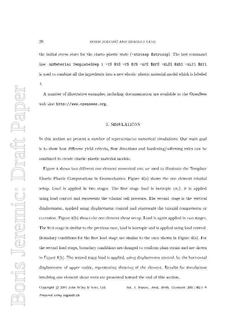
the initial stress state for the elasto{plastic state (-stressp $stressp). The last command

line nDMaterial Template3Dep 1 -YS $YS -PS $PS -EPS $EPS -ELS1 $ES1 -ELT1 $ET1

is used to combine all the ingredients into a new elastic{plastic material model which is labeled

1.

A number of illustrative examples, including documentation are available at the OpenSees

web site: http://www.opensees.org.

5. SIMULATIONS

In this section we present a number of representative numerical simulations. Our main goal

is to show how di�erent yield criteria, ow directions and hardening/softening rules can be

combined to create elastic{plastic material models.

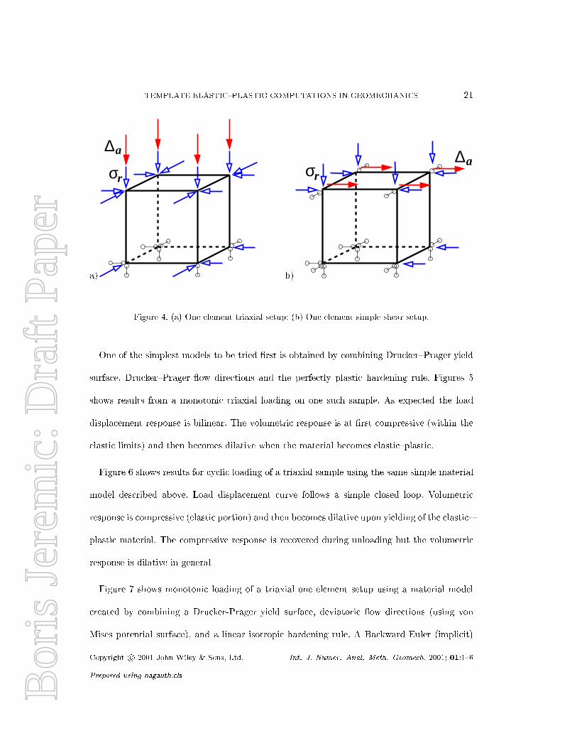
Figure 4 shows two di�erent one element numerical test we used to illustrate the Template

Elastic{Plastic Computations in Geomechanics. Figure 4(a) shows the one element triaxial

setup. Load is applied in two stages. The �rst stage load is isotropic (�r). it is applied

using load control and represents the triaxial cell pressure. The second stage is the vertical

displacement, applied using displacement control and represents the triaxial compression or

extension. Figure 4(b) shows the one element shear setup. Load is again applied in two stages.

The �rst stage is similar to the previous case, load is isotropic and is applied using load control.

Boundary conditions for the �rst load stage are similar to the ones shown in Figure 4(a). For

the second load stage, boundary conditions are changed to conform plain strain and are shown

in Figure 4(b). The second stage load is applied, using displacement control, by the horizontal

displacement of upper nodes, representing shearing of the element. Results for simulations

involving one element shear tests are presented toward the end of this section.



Bor

is J

erem

ic: D

raft

Pap


a)

σr

∆a

b)

σr

∆a

Figure 4. (a) One element triaxial setup; (b) One element simple shear setup.

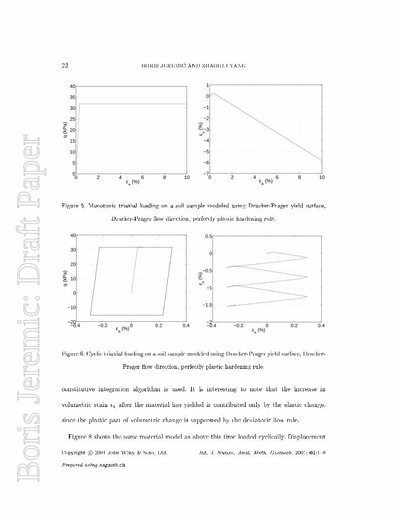
One of the simplest models to be tried �rst is obtained by combining Drucker{Prager yield

surface, Drucker{Prager ow directions and the perfectly plastic hardening rule. Figures 5

shows results from a monotonic triaxial loading on one such sample. As expected the load

displacement response is bilinear. The volumetric response is at �rst compressive (within the

elastic limits) and then becomes dilative when the material becomes elastic{plastic.

Figure 6 shows results for cyclic loading of a triaxial sample using the same simple material

model described above. Load displacement curve follows a simple closed loop. Volumetric

response is compressive (elastic portion) and then becomes dilative upon yielding of the elastic{

plastic material. The compressive response is recovered during unloading but the volumetric

response is dilative in general

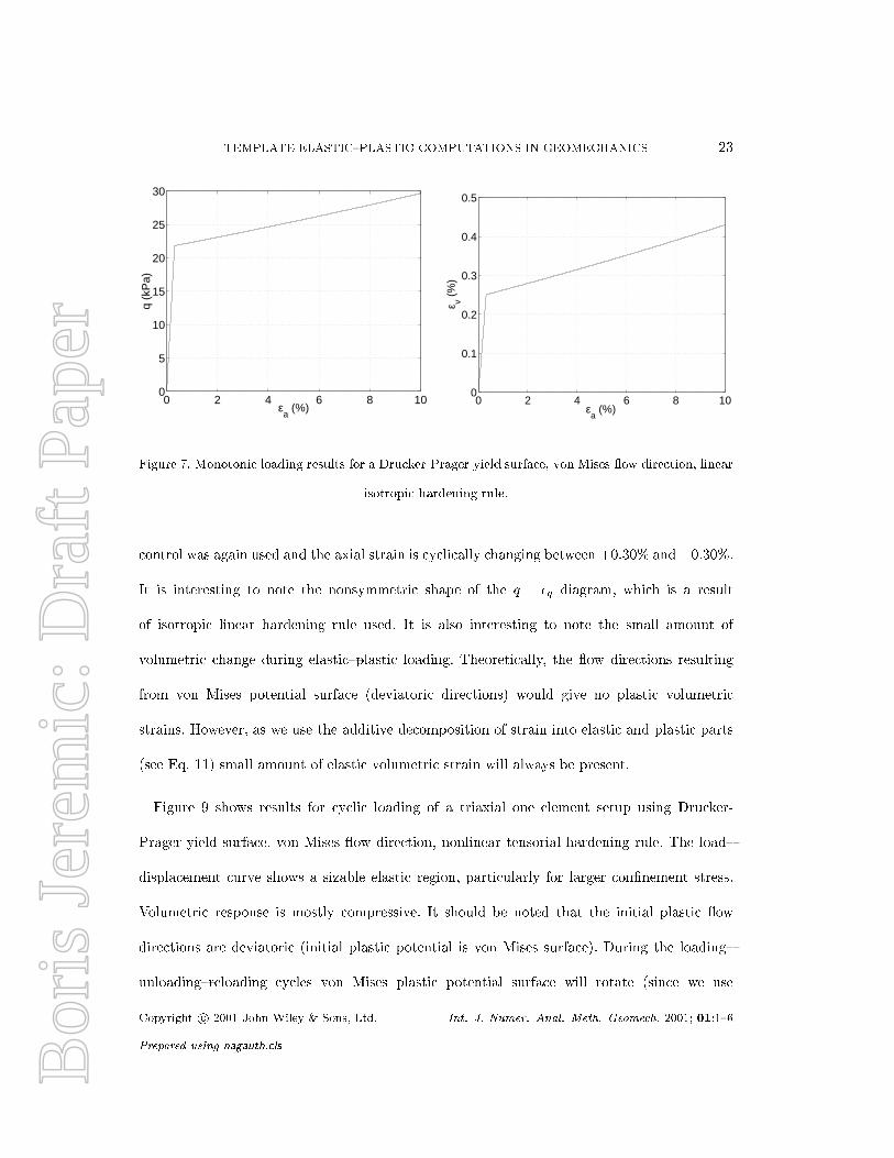
Figure 7 shows monotonic loading of a triaxial one element setup using a material model

created by combining a Drucker-Prager yield surface, deviatoric ow directions (using von

Mises potential surface), and a linear isotropic hardening rule. A Backward Euler (implicit)



Bor

is J

erem

ic: D

raft

Pap


0 2 4 6 8 100

5

10

15

20

25

30

35

40

εa (%)

q (k

Pa)

0 2 4 6 8 10−7

−6

−5

−4

−3

−2

−1

0

1

εa (%)

ε v (%

)Figure 5. Monotonic triaxial loading on a soil sample modeled using Drucker-Prager yield surface,

Drucker-Prager ow direction, perfectly plastic hardening rule.

−0.4 −0.2 0 0.2 0.4−20

−10

0

10

20

30

40

εa (%)

q (k

Pa)

−0.4 −0.2 0 0.2 0.4−2

−1.5

−1

−0.5

0

0.5

εa (%)

ε v (%

)

Figure 6. Cyclic triaxial loading on a soil sample modeled using Drucker-Prager yield surface, Drucker-

Prager ow direction, perfectly plastic hardening rule.

constitutive integration algorithm is used. It is interesting to note that the increase in

volumetric stain �v after the material has yielded is contributed only by the elastic change,

since the plastic part of volumetric change is suppressed by the deviatoric ow rule.

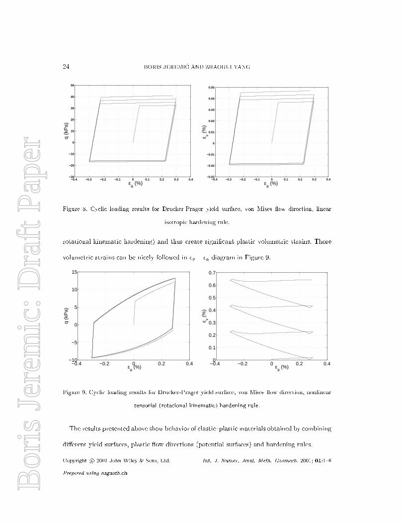
Figure 8 shows the same material model as above this time loaded cyclically. Displacement



Bor

is J

erem

ic: D

raft

Pap


0 2 4 6 8 100

5

10

15

20

25

30

εa (%)

q (k

Pa)

0 2 4 6 8 100

0.1

0.2

0.3

0.4

0.5

εa (%)

ε v (%

)Figure 7. Monotonic loading results for a Drucker-Prager yield surface, von Mises ow direction, linear

isotropic hardening rule.

control was again used and the axial strain is cyclically changing between +0:30% and �0:30%.

It is interesting to note the nonsymmetric shape of the q � �q diagram, which is a result

of isotropic linear hardening rule used. It is also interesting to note the small amount of

volumetric change during elastic{plastic loading. Theoretically, the ow directions resulting

from von Mises potential surface (deviatoric directions) would give no plastic volumetric

strains. However, as we use the additive decomposition of strain into elastic and plastic parts

(see Eq. 11) small amount of elastic volumetric strain will always be present.

Figure 9 shows results for cyclic loading of a triaxial one element setup using Drucker-

Prager yield surface, von Mises ow direction, nonlinear tensorial hardening rule. The load{

displacement curve shows a sizable elastic region, particularly for larger con�nement stress.

Volumetric response is mostly compressive. It should be noted that the initial plastic ow

directions are deviatoric (initial plastic potential is von Mises surface). During the loading{

unloading{reloading cycles von Mises plastic potential surface will rotate (since we use



Bor

is J

erem

ic: D

raft

Pap


−0.4 −0.3 −0.2 −0.1 0 0.1 0.2 0.3 0.4−30

−20

−10

0

10

20

30

40

50

εa (%)

q (k

Pa)

−0.4 −0.3 −0.2 −0.1 0 0.1 0.2 0.3 0.4−0.03

−0.02

−0.01

0

0.01

0.02

0.03

0.04

0.05

εa (%)

ε v (%

)Figure 8. Cyclic loading results for Drucker-Prager yield surface, von Mises ow direction, linear

isotropic hardening rule.

rotational kinematic hardening) and thus create signi�cant plastic volumetric strains. Those

volumetric strains can be nicely followed in �v � �a diagram in Figure 9.

−0.4 −0.2 0 0.2 0.4−10

−5

0

5

10

15

εa (%)

q (k

Pa)

−0.4 −0.2 0 0.2 0.40

0.1

0.2

0.3

0.4

0.5

0.6

0.7

εa (%)

ε v (%

)

Figure 9. Cyclic loading results for Drucker-Prager yield surface, von Mises ow direction, nonlinear

tensorial (rotational kinematic) hardening rule.

The results presented above show behavior of elastic{plastic materials obtained by combining

di�erent yield surfaces, plastic ow directions (potential surfaces) and hardening rules.



Bor

is J

erem

ic: D

raft

Pap


A more realistic response for soils can be obtained by combining above elements of an elastic{

plastic model with other, more sophisticated elements. For example, an excellent material

model for sand can be obtained by combining Drucker-Prager yield surface, Manzari-Dafalias

ow direction and bounding surface hardening rule (Manzari and Dafalias [28]).

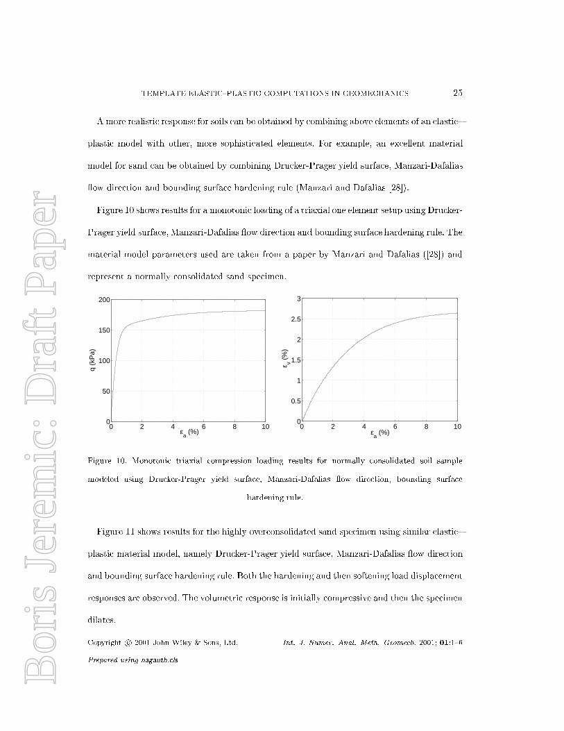
Figure 10 shows results for a monotonic loading of a triaxial one element setup using Drucker-

Prager yield surface, Manzari-Dafalias ow direction and bounding surface hardening rule. The

material model parameters used are taken from a paper by Manzari and Dafalias ([28]) and

represent a normally consolidated sand specimen.

0 2 4 6 8 100

50

100

150

200

εa (%)

q (k

Pa)

0 2 4 6 8 100

0.5

1

1.5

2

2.5

3

εa (%)

ε v (%

)

Figure 10. Monotonic triaxial compression loading results for normally consolidated soil sample

modeled using Drucker-Prager yield surface, Manzari-Dafalias ow direction, bounding surface

hardening rule.

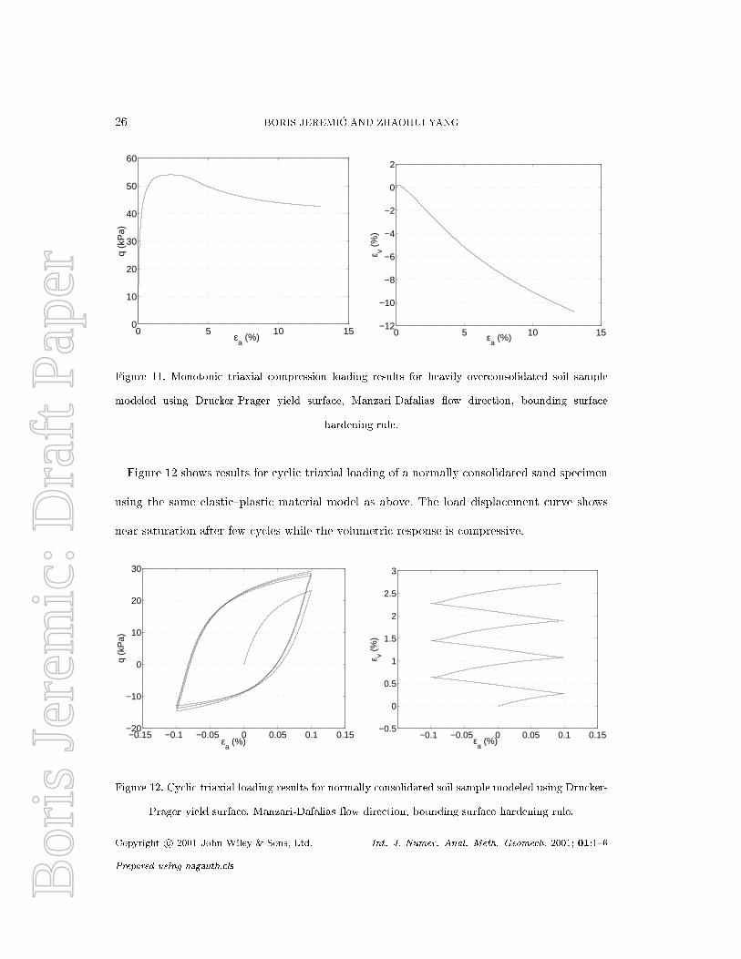
Figure 11 shows results for the highly overconsolidated sand specimen using similar elastic{

plastic material model, namely Drucker-Prager yield surface, Manzari-Dafalias ow direction

and bounding surface hardening rule. Both the hardening and then softening load displacement

responses are observed. The volumetric response is initially compressive and then the specimen

dilates.



Bor

is J

erem

ic: D

raft

Pap


0 5 10 150

10

20

30

40

50

60

εa (%)

q (k

Pa)

0 5 10 15−12

−10

−8

−6

−4

−2

0

2

εa (%)

ε v (%

)Figure 11. Monotonic triaxial compression loading results for heavily overconsolidated soil sample

modeled using Drucker-Prager yield surface, Manzari-Dafalias ow direction, bounding surface

hardening rule.

Figure 12 shows results for cyclic triaxial loading of a normally consolidated sand specimen

using the same elastic{plastic material model as above. The load displacement curve shows

near saturation after few cycles while the volumetric response is compressive.

−0.15 −0.1 −0.05 0 0.05 0.1 0.15−20

−10

0

10

20

30

εa (%)

q (k

Pa)

−0.1 −0.05 0 0.05 0.1 0.15−0.5

0

0.5

1

1.5

2

2.5

3

εa (%)

ε v (%

)

Figure 12. Cyclic triaxial loading results for normally consolidated soil sample modeled using Drucker-

Prager yield surface, Manzari-Dafalias ow direction, bounding surface hardening rule.



Bor

is J

erem

ic: D

raft

Pap


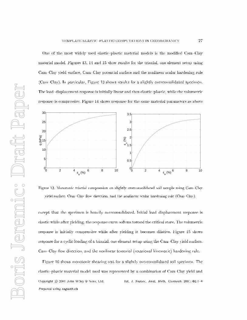
One of the most widely used elastic{plastic material models is the modi�ed Cam{Clay

material model. Figures 13, 14 and 15 show results for the triaxial, one element setup using

Cam{Clay yield surface, Cam{Clay potential surface and the nonlinear scalar hardening rule

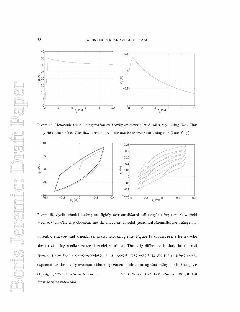
(Cam{Clay). In particular, Figure 13 shows results for a slightly overconsolidated specimen.

The load{displacement response is initially linear and then elastic{plastic, while the volumetric

response is compressive. Figure 14 shows response for the same material parameters as above

0 2 4 6 8 100

5

10

15

20

25

30

εa (%)

q (k

Pa)

0 2 4 6 8 100

0.5

1

1.5

2

2.5

3

3.5

εa (%)

ε v (%

)

Figure 13. Monotonic triaxial compression on slightly overconsolidated soil sample using Cam{Clay

yield surface, Cam{Clay ow direction, and the nonlinear scalar hardening rule (Cam{Clay).

except that the specimen is heavily overconsolidated. Initial load displacement response is

elastic while after yielding, the response curve softens toward the critical state. The volumetric

response is initially compressive while after yielding it becomes dilative. Figure 15 shows

response for a cyclic loading of a triaxial, one element setup using the Cam{Clay yield surface,

Cam{Clay ow direction, and the nonlinear tensorial (rotational kinematic) hardening rule.

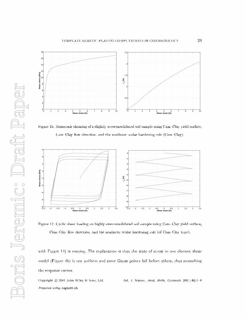
Figure 16 shows monotonic shearing test for a slightly overconoslidated soil specimen. The

elastic{plastic material model used was represented by a combination of Cam Clay yield and



Bor

is J

erem

ic: D

raft

Pap


0 2 4 6 8 100

5

10

15

20

25

30

35

40

εa (%)

q (k

Pa)

0 2 4 6 8 10−1

−0.5

0

0.5

εa (%)

ε v (%

)Figure 14. Monotonic triaxial compression on heavily overconsolidated soil sample using Cam{Clay

yield surface, Cam{Clay ow direction, and the nonlinear scalar hardening rule (Cam{Clay).

−0.4 −0.2 0 0.2 0.4−10

−5

0

5

10

εa (%)

q (k

Pa)

−0.4 −0.2 0 0.2 0.4−0.15

−0.1

−0.05

0

0.05

0.1

0.15

0.2

0.25

εa (%)

ε v (%

)

Figure 15. Cyclic triaxial loading on slightly overconsolidated soil sample using Cam{Clay yield

surface, Cam{Clay ow direction, and the nonlinear tensorial (rotational kinematic) hardening rule.

potential surfaces and a nonlinear scalar hardening rule. Figure 17 shows results for a cyclic

shear test using similar material model as above. The only di�erence is that the the soil

sample is now highly overconsolidated. It is interesting to note that the sharp failure point,

expected for the highly overconsolidated specimen modeled using Cam{Clay model (compare



Bor

is J

erem

ic: D

raft

Pap


0 1 2 3 4 5 6 7 8 9 100

2

4

6

8

10

12

14

16

18

Shear strain (%)

She

ar s

tres

s (k

Pa)

0 1 2 3 4 5 6 7 8 9 100

0.5

1

1.5

2

2.5

Shear strain (%)

ε v (%

)

Figure 16. Monotonic shearing of a slightly overconsolidated soil sample using Cam{Clay yield surface,

Cam{Clay ow direction, and the nonlinear scalar hardening rule (Cam{Clay).

−2.5 −2 −1.5 −1 −0.5 0 0.5 1 1.5 2 2.5−8

−6

−4

−2

0

2

4

6

8

Shear strain (%)

She

ar s

tres

s (k

Pa)

−2.5 −2 −1.5 −1 −0.5 0 0.5 1 1.5 2 2.5−10

−9

−8

−7

−6

−5

−4

−3

−2

−1

0

Shear strain (%)

ε v (%

)

Figure 17. Cyclic shear loading on highly overconsolidated soil sample using Cam{Clay yield surface,

Cam{Clay ow direction, and the nonlinear scalar hardening rule (of Cam{Clay type).

with Figure 14) is missing. The explanation is that the state of stress in one element shear

model (Figure 4b) is not uniform and some Gauss points fail before others, thus smoothing

the response curves.



Bor

is J

erem

ic: D

raft

Pap


6. CONCLUSIONS

In this paper we have presented a new approach to computations in elasto{plastic

geomechanics. The approach is based on the object oriented design philosophy and observations

on similarity of most incremental elastic{plastic material models. Based on this approach

we have shown that new elasto{plastic material models can be created by combining small

number of building blocks. This has an added bene�t of allowing an easy implementation

of other elastic{plastic material models based on the object oriented design principles. We

presented illustrative command language example used for creation of elastic{plastic models.

We also presented number of analysis results that emphasize features of template elastic{plastic

computations in geomechanics.

Last but not the least, we have made all of our developments, including source code, examples

and accompanying documentation in public domain, available at the OpenSees web site [33].

ACKNOWLEDGEMENT

This work was supported primarily by the Earthquake Engineering Research Centers Program of

the National Science Foundation under Award Number EEC-9701568. The authors wish to thank

Professor Gregory Fenves and Dr. Francis McKenna of University of California at Berkeley for helpful

discussion during the course of this work.



Bor

is J

erem

ic: D

raft

Pap


REFERENCES

1. ANSI ISO/IEC 14882-1998. Information Technology - Programming Languages - C++.

http://reality.sgi.com/austern_mti/std-c++/faq.html

2. G. C. Archer, G. Fenves, and C. Thewalt. A new object{oriented �nite element analysis program

architecture. Computers and Structures, 70(1):63{75, 1999.

3. Graham Charles Archer. Object Oriented Finite Analysis. PhD thesis, University of California, 1996.

4. P.J. Armstrong and C.O. Frederick. A mathematical representation of the multiaxial bauschinger e�ect.

Technical Report RD/B/N 731, C.E.G.B, 1966.

5. A. Baltov and A. Sawczuk. A rule of anisotropic hardening. Acta Mechanica, I(2):81{92, 1965.

6. Pompiliu Donescu and Tod A. Laursen. A generalized object{oriented approach to solving ordinary and

partial di�erential equations using �nite elements. Finite Elements in Analysis and Design, 22:93{107,

1996.

7. Yves Dubois-P�elerein and Thomas Zimmermann. Object{oriented �nite element programing: Iii. an

eÆcient implementation in c++. Computer Methods in Applied Mechanics and Engineering, 108:165{183,

1993.

8. Yves Dubois-P�elerin and Pierre Pegon. Object-oriented programming in nonlinear �nite element analysis.

Computers & Structures, 67(4):225{241, 1998.

9. J. M. Duncan and C.-Y Chang. Nonlinear analysis of stress and strain in soils. Journal of Soil Mechanics

and Foundations Division, 96:1629{1653, 1970.

10. D. Eyheramendy and Th. Zimmermann. Object{oriented �nite elements II. a symbolic environment for

automatic programming. Computer Methods in Applied Mechanics and Engineering, 132:277{304, 1996.

11. D. Eyheramendy and Th. Zimmermann. Object-oriented �nite elements. iv. symbolic derivations and

automatic programming of nonlinear formulations. Computer Methods in Applied Mechanics and

Engineering, 190(22-23):2729{2751, 2001.

12. Gregory L. Fenves. Object {oriented programming for engineering software development. Engineering

with Computers, 6:1{15, 1990.

13. R. Foerch, J. Besson, G Cailletaud, and P. Pilvin. Polymorphic constitutive equations in �nite element

codes. Computer methods in applied mechanics and engineering, 141:355{372, 1997.

14. Bruce W. R. Forde, Ricardo O. Foschi, and Siegfried F. Steimer. Object { oriented �nite element analysis.

Computers and Structures, 34(3):355{374, 1990.



Bor

is J

erem

ic: D

raft

Pap


15. B. O. Hardin. The nature of stress{strain behavior of soils. In Proceedings of the Specialty Conference

on Earthquake Engineering and Soil Dynamics, volume 1, pages 3{90, Pasadena, 1978.

16. N. Janbu. Soil compressibility as determined by odometer and triaxial tests. In Proceedings of European

Conference on Soil Mechanics and Foundation Engineering, pages 19{25, 1963.

17. Boris Jeremi�c, Kenneth Runesson, and Stein Sture. A model for elastic{plastic pressure sensitive materials

subjected to large deformations. International Journal of Solids and Structures, 36(31/32):4901{4918,

1999.

18. Boris Jeremi�c and Stein Sture. Implicit integrations in elasto{plastic geotechnics. International Journal

of Mechanics of Cohesive{Frictional Materials, 2:165{183, 1997.

19. Boris Jeremi�c and Stein Sture. Tensor data objects in �nite element programming. International Journal

for Numerical Methods in Engineering, 41:113{126, 1998.

20. H. W. Kuhn and A. W. Tucker. Nonlinear programming. In Jerzy Neyman, editor, Proceedings of the

Second Berkeley Symposium on Mathematical Statistics and Probability, pages 481 { 492. University of

California Press, July 31 { August 12 1950 1951.

21. Poul V. Lade. Double hardening constitutive model for soils, parameter determination and predictions

for two sands. In A. Saada and G. Bianchini, editors, Constitutive Equations for Granular Non{Cohesive

Soils, pages 367{382. A. A. Balkema, July 1988.

22. Poul V. Lade. E�ects of voids and volume changes on the behavior of frictional materials. International

Journal for Numerical and Analytical Methods in Geomechanics, 12:351{370, 1988.

23. Poul. V. Lade. Model and parameters for the elastic behavior of soils. In Swoboda, editor, Numerical

Methods in Geomechanics, pages 359{364, Innsbruck, 1988. Balkema, Rotterdam.

24. Poul V. Lade. Single{hardening model with application to NC clay. ASCE Journal of Geotechnical

Engineering, 116(3):394{414, 1990.

25. Poul V. Lade and Richard B. Nelson. Modeling the elastic behavior of granular materials. International

Journal for Numerical and Analytical Methods in Geomechanics, 4, 1987.

26. Jacob Lubliner. Plasticity Theory. Macmillan Publishing Company, New York., 1990.

27. Jaroslav Mackerle. Object{oriented techniques in FEM and BEM a bibliography (1996-1999). Finite

Elements in Analysis and Design, 36:189{196, 2000.

28. M. T. Manzari and Y. F. Dafalias. A critical state two{surface plasticity model for sands. G�eotechnique,

47(2):255{272, 1997.

29. Francis Thomas McKenna. Object Oriented Finite Element Programming: Framework for Analysis,



Bor

is J

erem

ic: D

raft

Pap


Algorithms and Parallel Computing. PhD thesis, University of California, 1997.

30. Ph. Men�entrey and Th. Zimmermann. Object{oriented non{linear �nite element analysis: Application to

J2 plasticity. Computers and Structures, 49(5):767{77, 1993.

31. Ph. Menetrey and K. J. Willam. Triaxial failure criterion for concrete and its generalization. ACI

Structural Journal, 92(3):311{318, May{June 1995.

32. G. R. Miller. An object { oriented approach to structural analysis and design. Computers and Structures,

40(1):75{82, 1991.

33. Open Source Project. OpenSees: open system for earthquake engineering simulations.

http://www.opensees.org; (to login use: user: guest, password OSg3OS).

34. M. Ortiz and E. P. Popov. Accuracy and stability of integration algorithms for elastoplastic constitutive

relations. International Journal for Numerical Methods in Engineering, 21:1561{1576, 1985.

35. John Ousterhout and Tcl/Tk Consortium. Tool command language (Tcl), tool kit (Tk) gui.

http://www.tclconsortium.org/ and http://www.scriptics.com/

36. R. M. V. Pidaparti and A. V. Hudli. Dynamic analysis of structures using object{oriented techniques.

Computers and Structures, 49(1):149{156, 1993.

37. K. H. Roscoe and J. B. Burland. On the generalized stress{strain behavior of wet clays. In J. Heyman

and F. A. Leckie, editors, Engineering Plasticity, pages 535{609, 1968.

38. K. H. Roscoe, A. N. Scho�eld, and A. Thurairajah. Yielding of clays in states wetter than critical.

G�eotechnique, 13(3):211{240, 1963.

39. K. H. Roscoe, A. N. Scho�eld, and C. P. Wroth. On the yielding of soils. Geotechnique, 8(1):22{53, 1958.

40. A. N. Scho�eld and C. P. Wroth. Critical State Soil Mechanics. McGraww{ Hill, 1968.

41. S.-P. Scholz. Elements of an object { oriented FEM++ program in C++. Computers and Structures,

43(3):517{529, 1992.

42. A. J. M. Spencer. Continuum Mechanics. Longman Mathematical Texts. Longman Group Limited, 1980.

43. S. Sture, K. Runesson, and E. J. Macari-Pasqualino. Analysis and calibration of a three invariant plasticity

model for granular materials. Ingenieur Archiv, 59:253{266, 1989.

44. I. Vardoulakis and J. Sulem. Bifurcation Analysis in Geomechanics. Blackie Academic & Professional,

1995. ISBN 0-7514-0214-1.

45. Gordon W. Zeglinski, Ray S. Han, and Peter Aitchison. Object oriented matrix classes for use in a �nite

element code using C++. International Journal for Numerical Methods in Engineering, 37:3921{3937,

1994.



Bor

is J

erem

ic: D

raft

Pap


46. Olgierd Cecil Zienkiewicz and Robert L. Taylor. The Finite Element Method, volume 1. McGraw - Hill

Book Company, fourth edition, 1991.

47. Th. Zimmermann and D. Eyheramendy. Object{oriented �nite elements I. principles of symbolic

derivations and automatic programming. Computer Methods in Applied Mechanics and Engineering,

132:259{276, 1996.

48. Thomas Zimmermann, Yves Dubois-P�elerin, and Patricia Bomme. Object oriented �nite element

programming: I. governing principles. Computer Methods in Applied Mechanics and Engineering, 98:291{

303, 1992.



TEMPLATE ELASTIC-PLASTIC COMPUTATIONS IN...

Documents

Transcript of TEMPLATE ELASTIC-PLASTIC COMPUTATIONS IN...