Tempered Particle Filtering - Federal Reserve System and Economics Discussion Series Divisions of...
67
Finance and Economics Discussion Series Divisions of Research & Statistics and Monetary Affairs Federal Reserve Board, Washington, D.C. Tempered Particle Filtering Edward Herbst and Frank Schorfheide 2016-072 Please cite this paper as: Herbst, Edward and Frank Schorfheide (2016). “Tempered Particle Filtering,” Finance and Economics Discussion Series 2016-072. Washington: Board of Governors of the Federal Reserve System, http://dx.doi.org/10.17016/FEDS.2016.072. NOTE: Staff working papers in the Finance and Economics Discussion Series (FEDS) are preliminary materials circulated to stimulate discussion and critical comment. The analysis and conclusions set forth are those of the authors and do not indicate concurrence by other members of the research staff or the Board of Governors. References in publications to the Finance and Economics Discussion Series (other than acknowledgement) should be cleared with the author(s) to protect the tentative character of these papers.
Transcript of Tempered Particle Filtering - Federal Reserve System and Economics Discussion Series Divisions of...

Finance and Economics Discussion SeriesDivisions of Research & Statistics and Monetary Affairs
Federal Reserve Board, Washington, D.C.
Tempered Particle Filtering
Edward Herbst and Frank Schorfheide
2016-072
Please cite this paper as:Herbst, Edward and Frank Schorfheide (2016). “Tempered Particle Filtering,” Finance andEconomics Discussion Series 2016-072. Washington: Board of Governors of the FederalReserve System, http://dx.doi.org/10.17016/FEDS.2016.072.
NOTE: Staff working papers in the Finance and Economics Discussion Series (FEDS) are preliminarymaterials circulated to stimulate discussion and critical comment. The analysis and conclusions set forthare those of the authors and do not indicate concurrence by other members of the research staff or theBoard of Governors. References in publications to the Finance and Economics Discussion Series (other thanacknowledgement) should be cleared with the author(s) to protect the tentative character of these papers.

Tempered Particle Filtering
Edward Herbst
Federal Reserve Board
Frank Schorfheide∗
University of Pennsylvania
PIER, CEPR, and NBER
August 25, 2016
Abstract
The accuracy of particle filters for nonlinear state-space models crucially depends
on the proposal distribution that mutates time t− 1 particle values into time t values.
In the widely-used bootstrap particle filter this distribution is generated by the state-
transition equation. While straightforward to implement, the practical performance is
often poor. We develop a self-tuning particle filter in which the proposal distribution is
constructed adaptively through a sequence of Monte Carlo steps. Intuitively, we start
from a measurement error distribution with an inflated variance, and then gradually
reduce the variance to its nominal level in a sequence of steps that we call tempering.
We show that the filter generates an unbiased and consistent approximation of the
likelihood function. Holding the run time fixed, our filter is substantially more accurate
in two DSGE model applications than the bootstrap particle filter.
JEL CLASSIFICATION: C11, C15, E10
KEY WORDS: Bayesian Analysis, DSGE Models, Nonlinear Filtering, Monte Carlo Methods
∗Correspondence: E. Herbst: Board of Governors of the Federal Reserve System, 20th Street and Con-
stitution Avenue N.W., Washington, D.C. 20551. Email: [email protected]. F. Schorfheide: De-
partment of Economics, 3718 Locust Walk, University of Pennsylvania, Philadelphia, PA 19104-6297. We
thank seminar participants at the Board of Governors and the Federal Reserve Bank of Cleveland for helpful
comments. Email: [email protected]. Schorfheide gratefully acknowledges financial support from the
National Science Foundation under the grant SES 1424843. The views expressed in this paper are those of
the authors and do not necessarily reflect the views of the Federal Reserve Board of Governors or the Federal
Reserve System.

1
1 Introduction
Estimated dynamic stochastic general equilibrium (DSGE) models are now widely used by
academics to conduct empirical research in macroeconomics as well as by central banks to
interpret the current state of the economy, to analyze the impact of changes in monetary
or fiscal policies, and to generate predictions for macroeconomic aggregates. In most ap-
plications, the estimation utilizes Bayesian techniques, which require the evaluation of the
likelihood function of the DSGE model. If the model is solved with a (log)linear approx-
imation technique and driven by Gaussian shocks, then the likelihood evaluation can be
efficiently implemented with the Kalman filter. If, however, the DSGE model is solved using
a nonlinear technique, the resulting state-space representation is nonlinear and the Kalman
filter can no longer be used.
Fernandez-Villaverde and Rubio-Ramırez (2007) proposed to use a particle filter to evalu-
ate the likelihood function of a nonlinear DSGE model and many other papers have followed
this approach since. However, configuring the particle filter so that it generates an accurate
approximation of the likelihood function remains a key challenge. The contribution of this
paper is to propose a self-tuning particle filter, which we call a tempered particle filter, that
in our applications is substantially more accurate than the widely-used bootstrap particle
filter.
Our starting point is the state-space representation of a potentially nonlinear DSGE
model given by a measurement equation and a state-transition equation the form
yt = Ψ(st, t; θ) + ut, ut ∼ N(0,Σu(θ)
)(1)
st = Φ(st−1, εt; θ), εt ∼ Fε(·; θ).
The functions Ψ(st, t; θ) and Φ(st−1, εt; θ) are generated numerically when solving the DSGE
model. Here yt is a ny× 1 vector of observables, ut is a ny× 1 vector of normally distributed
measurement errors, and st is an ns × 1 vector of hidden states. In order to obtain the
likelihood increments p(yt+1|Y1:t, θ), where Y1:t = {y1, . . . , yt}, it is necessary to integrate out
the latent states:
p(yt+1|Y1:t, θ) =
∫ ∫p(yt+1|st+1, θ)p(st+1|st, θ)p(st|Y1:t, θ)dst+1dst, (2)
which can be done recursively with a filter.

2
Particle filters represent the distribution of the hidden state vector st conditional on time
t information Y1:t = {y1, . . . , yt} through a swarm of particles {sjt ,W jt }Mj=1 such that
1
M
M∑j=1
h(sjt)Wjt ≈
∫h(st)p(st|Y1:t, θ). (3)
The approximation here is in the sense of a strong law of large numbers (SLLN) or a central
limit theorem (CLT). The approximation error vanishes as the number of particles M tends
to infinity. The filter recursively generates approximations of p(st|Y1:t, θ) for t = 1, . . . , T
and produces approximations of the likelihood increments p(yt|Y1:t, θ) as a by-product. There
exists a large literature on particle filters. Surveys and tutorials are provided, for instance,
by Arulampalam, Maskell, Gordon, and Clapp (2002), Cappe, Godsill, and Moulines (2007),
Doucet and Johansen (2011), Creal (2012), and Herbst and Schorfheide (2015). Textbook
treatments of the statistical theory underlying particle filters can be found in Liu (2001),
Cappe, Moulines, and Ryden (2005), and Del Moral (2013).
The conceptually most straightforward version of the particle filter is the bootstrap par-
ticle filter proposed by Gordon, Salmond, and Smith (1993). This filter uses the state-
transition equation to turn sjt−1 particles onto sjt particles, which are then reweighted based
on their success in predicting the time t observation, measured by p(yt|sjt , θ). While the
bootstrap particle filter is easy to implement, it relies on the state-space model’s ability to
accurately predict yt by forward simulation of the state-transition equation. In general, the
lower the average density p(yt|sjt , θ), the more uneven the distribution of the updated particle
weights, and the less accurate the approximation in (3).
Ideally, the proposal distribution for sjt should not just be based on the state-transition
equation p(st|st−1, θ), but also account for the observation yt. In fact, conditional on sjt−1
the optimal proposal distribution is the posterior
p(st|yt, sjt−1, θ) ∝ p(yt|st, θ)p(st|sjt−1, θ),
where ∝ denotes proportionality. Unfortunately, in a generic nonlinear state-space model, it
is not possible to directly sample from this distribution. Constructing an approximation for
p(st|yt, sjt−1, θ) in a generic state-space model is difficult and often involves tedious model-
specific calculations that have to be executed by the user of the algorithm prior to its
implementation.1 The innovation in our paper is to generate this approximation in a sequence
1Attempts include approximations based on the one-step Kalman filter updating formula applied to a

3
of Monte Carlo steps. The starting point is the observation, that the larger the measurement
error variance the more accurate the filter becomes, because holding everything else constant,
the variance of the particle weights decreases. Building on this insight, in each period t,
we generate sjt by forward simulation, but then update the particle weights based on a
density p1(yt|st, θ) with an inflated measurement error variance. In a sequence of steps that
we call tempering, we reduce this inflated measurement error variance to its nominal level.
These steps mimic a sequential Monte Carlo algorithm designed for a static parameter. Such
algorithms have been successfully used to approximate posterior distributions for parameters
of econometric models.2
We show that our proposed tempered particle filter produces a valid approximation of the
likelihood function and substantially reduces the Monte Carlo error relative to the bootstrap
particle filter, even after controlling for computational time. Our algorithm can be embed-
ded into particle Markov chain Monte Carlo algorithms that replace the true likelihood by
a particle-filter approximation; see, for instance, Fernandez-Villaverde and Rubio-Ramırez
(2007) for DSGE model applications and Andrieu, Doucet, and Holenstein (2010) for the
underlying statistical theory.
The remainder of the paper is organized as follows. The proposed tempered particle
filter is presented in Section 2. We provide a SLLN for the particle filter approximation of
the likelihood function in Section 3 and show that the approximation is unbiased. Here we
are focusing of a version of the filter that is non-adaptive. The filter is applied to a small-
scale New Keynesian DSGE model and the Smets-Wouters model in Section 4 and Section 5
concludes. Theoretical derivations, computational details, DSGE model descriptions, and
data sources are relegated to the Online Appendix.
2 The Tempered Particle Filter
A key determinant of the behavior of a particle filter is the distribution of the normalized
weights
W jt =
wjtWjt−1
1M
∑Mi=1 w
jtW
jt−1
,
linearized version of the DSGE model. Alternatively, one could use the updating step of an approximatefilter, e.g., the ones developed by Andreasen (2013) or Kollmann (2015).
2Chopin (2002) first showed how to use sequential Monte Carlo methods to conduct inference on aparameter that does not evolve over time. Applications to the estimation of DSGE model parametershave been considered in Creal (2007) and Herbst and Schorfheide (2014). Durham and Geweke (2014) andBognanni and Herbst (2015) provide applications to the estimation of other time-series models.

4
where W jt−1 is the (normalized) weight associated with the jth particle at time t − 1, wjt
incremental weight after observing yt, and W jt is the normalized weight accounting for this
new observation.3 For the bootstrap particle filter, the incremental weight is simply the
likelihood of observing yt given the jth particle, p(yt|sjt , θ).
One can show that, holding the observations fixed, the bootstrap particle filter becomes
more accurate as the measurement error variance increases because the variance of the par-
ticle weights {Wt}Mj=1 decreases. Consider the following stylized example which examines
an approximate population analogue for W jt . Suppose that yt is scalar, the measurement
errors are distributed as ut ∼ N(0, σ2u), Wt−1 = 1, and let δt = yt − Ψ(st, t; θ). Moreover,
assume that in population the δt’s are distributed according to a N(0, 1). In this case, we
can define the weights v(δt) normalized under the population distribution of δt as (omitting
t subscripts):
v(δ) =exp
{− 1
2σ2uδ2}
(2π)−1/2∫
exp{−1
2
(1 + 1
σ2u
)δ2}dδ
=
(1 +
1
σ2u
)1/2
exp
{− 1
2σ2u
δ2
}.
By virtue of the normalization, the mean of the weights is equal to one: E[v(δ)] = 1.
The population variance of the weights v(δ) is given by
V[v(δ)] =
∫v2(δ)dδ − 1 =
1
σu
1 + σ2u√
2 + σ2u
− 1.
Note that V[v(δ)] −→ ∞ as σu −→ 0. Moreover, V[v(δ)] −→ 0 as σu −→ ∞. By differenti-
ating with respect to σu one can show that the variance is monotonically decreasing in the
measurement error variance σ2u. This heuristic illustrates that the larger the measurement
error variance in the state-space model (holding the observations fixed), the smaller the vari-
ance of the particle weights. Because the variance of an importance sampling approximation
is an increasing function of the variance of the particle weights, increasing the measurement
error variance tends to raise the accuracy of the particle filter approximation.
We use this insight to construct a tempered particle filter in which we generate proposed
particle values sjt sequentially, by reducing the measurement error variance from an inflated
3In the notation developed subsequently, the tilde on W jt indicates that this is weight associated with
particle j before any resampling of the particles.

5
initial level Σu(θ)/φ1 to the nominal level Σu(θ). Formally, define
pn(yt|st, θ) ∝ φd/2n |Σu(θ)|−1/2 exp
{−1
2(yt −Ψ(st, t; θ))
′φnΣ−1u (θ)(yt −Ψ(st, t; θ))
}, (4)
where:
φ1 < φ2 < . . . < φNφ = 1.
Here φn scales the inverse covariance matrix of the measurement error and can therefore be
interpreted as a precision parameter. The reduction of the measurement error variance is
achieved by a sequence of Monte Carlo steps that we borrow from the literature of SMC
approximations for posterior moments of static parameters (see Chopin (2002) and, for
instance, the treatment in Herbst and Schorfheide (2015)).
By construction, pNφ(yt|st, θ) = p(yt|st, θ). Based on pn(yt|st, θ) we can define the bridge
distributions
pn(st|yt, st−1, θ) ∝ pn(yt|st, θ)p(st|st−1, θ). (5)
Integrating out st−1 under the distribution p(st−1|Y1:t−1, θ) yields the bridge posterior density
for st conditional on the observables:
pn(st|Y1:t, θ) =
∫pn(st|yt, st−1, θ)p(st−1|Y1:t−1, θ)dst−1. (6)
In the remainder of this section we describe the proposed tempered particle filter. We do so
in two steps: Section 2.1 presents the main algorithm that iterates over periods t = 1, . . . , T
to approximate the likelihood increments p(yt|Y1:t−1, θ) and the filtered states p(st|Y1:t, θ).
In Section 2.2 we focus on the novel component of our algorithm, which in every period t
uses Nφ steps to reduce the measurement error variance from Σu(θ)/φ1 to Σu(θ).
2.1 The Main Iterations
The tempered particle filter has the same structure as the bootstrap particle filter. In
every period t, we use the state-transition equation to simulate the state vector forward, we
update the particle weights, and we resample the particles. The key innovation is to start
out with a fairly large measurement error variance, which is then iteratively reduced to the
nominal measurement error variance Σu(θ). As the measurement error variance is reduced

6
(tempering), we adjust the innovations to the state-transition equation as well as the particle
weights. The algorithm is essentially self-tuning. The user only has to specify the overall
number of particles M and two tuning parameters for the tempering steps. The tempering
sequence φ1, . . . , φNφ can be chosen adaptively. We will provide more details in Section 2.2.
Algorithm 1 summarizes the iterations over periods t = 1, . . . , T .
Algorithm 1 (Tempered Particle Filter)
1. Period t = 0 initialization. Draw the initial particles from the distribution sj0iid∼
p(s0|θ) and set Nφ = 1, sj,Nφ0 = sj0, and W
j,Nφ0 = 1, j = 1, . . . ,M .
2. Period t Iterations. For t = 1, . . . , T :
(a) Particle Initialization.
i. Starting from {sj,Nφt−1 ,Wj,Nφt−1 }, generate εj,1t ∼ Fε(·; θ) and define
sj,1t = Φ(sj,Nφt−1 , ε
j,1t ; θ).
ii. Compute the incremental weights:
wj,1t = p1(yt|sj,1t , θ) (7)
= (2π)−d/2φd/21 |Σu(θ)|−1/2
×[exp
{− 1
2
(yt −Ψ(sj,1t , t; θ)
)′φ1Σ−1
u (θ)(yt −Ψ(sj,1t , t; θ)
)}].
iii. Normalize the incremental weights:
W j,1t =
wj,1t Wj,Nφt−1
1M
∑Mj=1 w
j,1t W
j,Nφt−1
(8)
to obtain the particle swarm {sj,1t , εj,1t , sj,Nφt−1 , W
j,1t }, which leads to the approx-
imation
h1t,M =
1
M
M∑j=1
h(sj,1t )W j,1t ≈
∫h(st)p1(st|Y1:t, θ)dst. (9)
Moreover1
M
M∑j=1
wj,1t Wj,Nφt−1 ≈ p1(yt|Y1:t−1, θ). (10)

7
iv. Resample the particles:
{sj,1t , εj,1t , sj,Nφt−1 , W
j,1t } 7→ {sj,1t , εj,1t , s
j,Nφt−1 ,W
j,1t },
where W j,1t = 1 for j = 1, . . . , N . This leads to the approximation
h1t,M =
1
M
M∑j=1
h(sj,1t )W j,1t ≈
∫h(st)p1(st|Y1:t)dst. (11)
(b) Tempering Iterations: Execute Algorithm 2 to
i. convert the particle swarm
{sj,1t , εj,1t , sj,Nφt−1 ,W
j,1t } 7→ {sj,Nφt , ε
j,Nφt , s
j,Nφt−1 ,W
j,Nφt }
to approximate
hNφt,M =
1
M
M∑j=1
h(sj,Nφt )W
j,Nφt ≈
∫h(st)p(st|Y1:t, θ)dst; (12)
ii. compute the approximation pM(yt|Y1:t−1, θ) of the likelihood increment.
3. Likelihood Approximation
pM(Y1:T |θ) =T∏t=1
pM(yt|Y1:t−1, θ). � (13)
If we were to set φ1 = 1, Nφ = 1, and omit Step 2.(b), then Algorithm 1 is exactly
identical to the bootstrap particle filter: the sjt−1 particle values are simulated forward using
the state-transition equation, the weights are then updated based on how well the new state
sjt predicts the time t observations, measured by the predictive density p(yt|sjt), and finally
the particles are resampled using a standard resampling algorithm, such as multinominal
resampling, or systematic resampling.4
The drawback of the bootstrap particle filter is that the proposal distribution for the
innovation εjt ∼ Fε(·; θ) is “blind,” in that it is not adapted to the period t observation yt.
This typically leads to a large variance in the incremental weights wjt , which in turn translates
4Detailed textbook treatments of resampling algorithms can be found in the by Liu (2001) and Cappe,Moulines, and Ryden (2005).

8
into inaccurate Monte Carlo approximations. Taking the states {sjt−1}Mj=1 as given and
assuming that a t− 1 resampling step has equalized the particle weights, that is, W jt−1 = 1,
the conditionally optimal choice for the proposal distribution is p(εjt |sjt−1, yt, θ). However,
because of the nonlinearity in state-transition and measurement equation, it is not possible
to directly generate draws from this distribution. The main idea of our algorithm is to
sequentially adapt the proposal distribution for the innovations to the current observation
yt by raising φn from a small initial value to φNφ = 1.5 This is done in Step 2(b), which is
described in detail in Algorithm 2 in the next section.
In general, we could replace the draws of εj,1t from the innovation distribution Fε(·; θ) in
Step 2(a)i of Algorithm 2 with draws from a tailored distribution with density g1t (ε
j,1t |s
j,Nφt−1 )
and then adjust the incremental weight ωj,1t by the ratio pε(εj,1t )/g1
t (εj,1t |s
j,Nφt−1 ), as it is done
in the generalized version of the particle filter. Here the gt(·) density might be constructed
based on a linearized version of the DSGE model or be obtained through the updating steps
of a conventional nonlinear filter, such as an extended Kalman filter, unscented Kalman filter,
or a Gaussian quadrature filter. Thus, the proposed tempering steps can be used either to
relieve the user from the burden of having to construct a g1t (ε
j,1t |s
j,Nφt−1 ) in the first place; or it
could be used to improve upon the accuracy obtained with a readily-available g1t (ε
j,1t |s
j,Nφt−1 ).
2.2 Tempering the Measurement Error Variance
The tempering iterations build on the sequential Monte Carlo (SMC) algorithms that have
been developed for static parameters. In these algorithms (see, for instance, Chopin (2002),
Durham and Geweke (2014), Herbst and Schorfheide (2014, 2015)), the goal is to generate
draws from a posterior distribution p(θ|Y ) by sampling from a sequence of bridge posteriors
pn(θ|Y ) ∝[p(Y |θ)
]φnp(θ). Note that the bridge posterior is equal to the actual posterior
for φn = 1. At each iteration, the algorithm cycles through three stages: particle weights
are updated in the correction step; the particles are being resampled and particle weights
are equalized in the selection step; and particle values are changed in the mutation step.
The analogue of[p(Y |θ)
]φnin our algorithm is pn(yt|st, θ) given in (4), which reduces to
p(yt|st, θ) for φn = 1. Algorithm 2 summarizes the correction, selection, and mutation steps
for tempering iterations n = 2, . . . , Nφ.
5The number of iterations that we are using depends on the period t, but to simplify the notationsomewhat, we dropped the t subscript and write Nφ rather than Nφ,t.

9
Algorithm 2 (Tempering Iterations) This algorithm receives as input the particle swarm
{sj,1t , εj,1t , sj,Nφt−1 ,W
j,1t } and returns as output the particle swarm {sj,Nφt , ε
j,Nφt , s
j,Nφt−1 ,W
j,Nφt } and
the likelihood increment pM(yt|Y1:t−1, θ). Set n = 2 and Nφ = 0.
1. Do until n = Nφ:
(a) Correction:
i. For j = 1, . . . ,M define the incremental weights
wj,nt (φn) =pn(yt|sj,n−1
t , θ)
pn−1(yt|sj,n−1t , θ)
(14)
=
(φnφn−1
)d/2exp
{− 1
2
[yt −Ψ(sj,n−1
t , t; θ)]′
×(φn − φn−1)Σ−1u
[yt −Ψ(sj,n−1
t , t; θ)]}.
ii. Define the normalized weights
W j,nt (φn) =
wj,nt (φn)W j,n−1t
1M
∑Mj=1 w
j,nt (φn)W j,n−1
t
, (15)
(W j,n−1t = 1, because the resampling step was executed in iteration n − 1),
and the inefficiency ratio
InEff(φn) =1
M
M∑j=1
(W j,nt (φn)
)2. (16)
iii. If InEff(φn = 1) ≤ r∗, then set φn = 1, Nφ = n, and W j,nt = W j,n
t (φn = 1).
Otherwise, let n = n + 1, φ∗n be the solution to InEff(φ∗n) = r∗, and W j,nt =
W j,nt (φn = φ∗n).
iv. The particle swarm {sj,n−1t , εj,n−1
t , sj,Nφt−1 , W
j,nt } approximates
hnt,M =1
M
M∑j=1
h(sj,n−1t )W j,n
t ≈∫h(st)pn(st|Y1:t, θ)dst. (17)
(b) Selection: Resample the particles:
{sj,n−1t , εj,n−1
t , sj,Nφt−1 , W
j,nt } 7→ {sj,nt , εj,nt , s
j,Nφt−1 ,W
j,nt },

10
where W j,nt = 1 for j = 1, . . . , N . Keep track of the correct ancestry information
such that
sj,nt = Φ(sj,Nφt−1 , ε
j,nt ; θ)
for each j. This leads to the approximation
hnt,M =1
M
M∑j=1
h(sj,nt )W j,nt ≈
∫h(st)pn(st|Y1:t, θ)dst. (18)
(c) Mutation: Use a Markov transition kernel Kn(st|st; st−1) with the invariance
property
pn(st|yt, st−1, θ) =
∫Kn(st|st; st−1)pn(st|yt, st−1, θ)dst (19)
to mutate the particle values (see Algorithm 3 for an implementation). This leads
to the particle swarm {sj,nt , εj,nt , sj,Nφt−1 ,W
j,nt }, which approximates
hnt,M =1
M
M∑j=1
h(sj,nt )W j,nt ≈
∫h(st)pn(st|Y1:t, θ)dst. (20)
2. Approximate the likelihood increment:
pM(yt|Y1:t−1, θ) =
Nφ∏n=1
(1
M
M∑j=1
wj,nt W j,n−1t
)(21)
with the understanding that W j,0t = W
j,Nφt−1 . �
The correction step adapts the stage n − 1 particle swarm to the reduced measurement
error variance in stage n by reweighting the particles. The incremental weights in (14) capture
the change in the measurement error variance from Σn(θ)/φn−1 to Σn(θ)/φn and yield an
importance sampling approximation of pn(st|Y1:t, θ) based on the stage n− 1 particle values.
Rather than relying on a fixed exogenous tempering schedule {φn}Nφn=1, we choose φn to
achieve a targeted inefficiency ratio r∗ > 1, an approach that has proven useful in the context
of global optimization of nonlinear functions. Geweke and Frischknecht (2014) develop an
adaptive SMC algorithm incorporating targeted tempering to solve such problems. To relate
the inefficiency ratio to φn, we begin by defining
ej,t =1
2(yt −Ψ(sj,n−1
t , t; θ))′Σ−1u (yt −Ψ(sj,n−1
t , t; θ)).

11
Assuming that the particles were resampled in iteration n− 1 and W j,n−1t = 1, we can then
express the inefficiency ratio as
InEff(φn) =1
M
M∑j=1
(W j,nt (φn)
)2=
1M
∑Mj=1 exp[−2(φn − φn−1)ej,t](
1M
∑Mj=1 exp[−(φn − φn−1)ej,t]
)2 . (22)
It is straightforward to verify that for φn = φn−1 the inefficiency ratio InEff(φn) = 1 < r∗.
Moreover, we show in the Online Appendix that the function is monotonically increasing
on the interval [φn−1, 1], which is the justification for Step 1(a)iii of Algorithm 3. Thus, we
are raising φn as closely to one as we can without exceeding a user-defined bound on the
variance of the particle weights. Note that we can use the same approach to set the initial
scaling factor φ1 in Algorithm 1.
The selection step is executed in every iteration n to ensure that we can find a unique
φn+1 based on (22) in the subsequent iteration. The equalization of the particle weights
allows us to characterize the properties of the function InEff(φn). Finally, in the mutation
step we are using a Markov transition kernel to change the particle values (sj,nt , εj,nt ) in a
way to maintain an approximation of pn(st|Y1:t, θ). In the absence of the mutation step the
initial particle values (sj,1t , εj,1t ) generated in Step 2(a) of Algorithm 2 would never change
and we would essentially reproduce the bootstrap particle filter by computing p(yt|sjt , θ)sequentially under a sequence of measurement error covariance matrices that converges to
Σu(θ). The mutation can be implemented with NMH steps of a random walk Metropolis-
Hastings (RWMH) algorithm.
Algorithm 3 (RWMH Mutation Step) This algorithm receives as input the particle swarm
{sj,nt , εj,nt , sj,Nφt−1 ,W
j,nt } and returns as output the particle swarm {sj,nt , εj,nt , s
j,Nφt−1 ,W
j,nt }.
1. Tuning of Proposal Distribution: Compute
µεn =1
M
M∑j=1
εj,nt W j,nt , Σε
n =1
M
M∑j=1
εj,nt (εj,nt )′W j,nt − µεn(µεn)′.
2. Execute NMH Metropolis-Hastings Steps for Each Particle: For j = 1, . . .M :
(a) Set εj,n,0t = εj,nt . Then, for l = 1, . . . , NMH :

12
i. Generate a proposed innovation:
ejt ∼ N(εj,n,l−1t , c2
nΣεn
).
ii. Compute the acceptance rate:
α(ejt |εj,n,l−1t ) = min
{1,
pn(yt|ejt , sj,Nφt−1 , θ)pε(e
jt)
pn(yt|εj,n,l−1t , s
j,Nφt−1 , θ)pε(ε
j,n,l−1t )
}.
iii. Update particle values:
εj,n,lt =
{ejt with prob. α(ejt |εj,n,l−1
t )
εj,n,l−1t with prob. 1− α(ejt |εj,n,l−1
t )
(b) Define
εj,nt = εj,n,NMHt , sj,nt = Φ(s
j,Nφt−1 , ε
j,nt ; θ). �
To tune the RWMH steps, we use the {εj,nt ,W j,nt } particles (this is the output from the
selection step in Algorithm 2) to compute a covariance matrix for the Gaussian proposal
distribution used in Step 2.(a) of Algorithm 3. We scale the covariance matrix adaptively
by cn to achieve a desired acceptance rate. In particular, we compute the average empirical
rejection rate Rn−1(cn−1), based on the Mutation phase in iteration n − 1. The average is
computed across the NMH RWMH steps. We set c1 = c∗ and for n > 2 adjust the scaling
factor according to
cn = cn−1f(1− Rn−1(cn−1)
), f(x) = 0.95 + 0.10
e20(x−0.40)
1 + e20(x−0.40). (23)
This function is designed to increase the scaling factor by 5 percent if the acceptance rate
is well above 0.40, and decrease the scaling factor by 5 percent if the acceptance rate is well
below 0.40. For acceptance rates near 0.40, the increase (or decrease) of cn is attenuated by
the logistic component of the function above. In our empirical applications, the performance
of the filter was robust to variations on the rule.
In order to run Algorithm 3 the user has to specify the initial scaling of the proposal
covariance matrix c∗, as well as the number of Metropolis-Hastings steps. In principle, the
user can also adjust the target acceptance rate and the speed of adjustment in (23).

13
3 Theoretical Properties of the Filter
We will now examine asymptotic (with respect to the number of particles M) and finite sam-
ple properties of the particle filter approximation of the likelihood function. Section 3.1 pro-
vides a SLLN and Section 3.2 shows that the likelihood approximation is unbiased. Through-
out this section, we will focus on a version of the filter that is not self-tuning. This version
of the filter replaces Algorithm 2 by Algorithm 4 and Algorithm 3 by Algorithm 5:
Algorithm 4 (Tempering Iterations – Not Self-Tuning) This algorithm is identical to
Algorithm 2, with the exception that the tempering schedule {φn}Nφn=1 is pre-determined. The
Do until n = Nφ-loop is replaced by a For n = 1 to Nφ-loop and Step 1(a)iii is eliminated. �
Algorithm 5 (RWMH Mutation Step – Not Self-Tuning) This algorithm is identi-
cal to Algorithm 3 with the exception that the sequences {cn,Σεn}
Nφn=1 are pre-determined.
�
Extensions of the asymptotic results to self-tuning sequential Monte Carlo algorithms are
discussed, for instance, in Herbst and Schorfheide (2014) and Durham and Geweke (2014).
3.1 Asymptotic Properties
Under suitable regularity conditions the Monte Carlo approximations generated by a particle
filter satisfy a SLLN and a CLT. Proofs for a generic particle filter are provided in Chopin
(2004). We will subsequently establish a SLLN for the tempered particle filter, by modifying
the recursive proof developed by Chopin (2004) to account for the tempering iterations of
Algorithm 4. To simplify the notation we drop θ from the conditioning set of all densities.
In this paper we are primarily interested in establishing an almost-sure limit for the Monte
Carlo approximation of the likelihood function:
pM(Y1:T ) =T∏t=1
pM(yt|Y1:t−1)a.s.−→
T∏t=1
p1(yt|Y1:t−1)
Nφ∏n=2
pn(yt|Y1:t−1)
pn−1(yt|Y1:t−1)
= p(Y1:T ). (24)
Here the last equality follows because pNφ(yt|Y1:t−1) = p(yt|Y1:t−1) by definition. The limit
is obtained by letting the number of particles M −→ ∞. We assume that the length of the

14
sample T is fixed. As a by-product, we also derive an almost-sure limit for Monte Carlo
approximations of moments of the filtered states:
hnt,M =1
M
M∑j=1
h(sj,nt , sj,Nφt−1 )W j,n
ta.s.−→
∫ ∫h(st, st−1)pn(st, st−1|Y1:t)dstdst−1. (25)
We use h(·) to denote a generic function of both st and st−1 for technical reasons that will
be explained below.6 Of course, a special case is a function that is constant with respect to
st−1. For short, we simply denote such functions by h(st).
In order to guarantee the almost-sure convergence, we need to impose some regularity
conditions on the functions h(st, st−1). We define the following classes of functions:
H1t =
{h(st, st−1)
∣∣∣∣ ∫ Ep(·|st−1)[|h(st, st−1)|]p(st−1|Y1:t−1)dst−1 <∞, (26)
∃δ > 0 s.t. Ep(·|st−1)
[∣∣h(st, st−1)− Ep(·|st−1)[h]∣∣1+δ
]< C <∞,
Ep(·|st−1)[h] ∈ HNφt−1
}and for n = 2, . . . , Nφ:
Hnt =
{h(st, st−1)
∣∣∣∣h(st, st−1) ∈ Hn−1t , (27)
∃δ > 0 s.t. EKn(·|st,st−1)
[∣∣h(st, st−1)− EKn(·|st,st−1)[h]∣∣1+δ
]< C <∞,
EKn(·|st,st−1)[h(st, st−1)] ∈ Hn−1t
}.
By definition Hnt ⊆ Hn
t for n > n. The classes Hnt are chosen such that the moment bounds
that guarantee the almost sure convergence of Monte Carlo averages of h(sj,nt , sj,Nφt−1 ) are
satisfied. The key assumption here is that there exists a uniform bound for the centered 1+δ
conditional moment of the function h(st, st−1) under the state-transition density p(st|st−1)
and the transition kernel of the mutation step of Algorithm 5, Kn(st|st, st−1). This will allow
us to apply a SLLN to the particles generated by the forward simulation of the model and
the mutation step in the tempering iterations.
6Spoiler alert: we need the st−1 because the Markov transition kernel generated by Algorithm 4 (orAlgorithm 2 is invariant under the distribution pn(st|yt, st−1), which is conditioned on st−1, instead of thedistribution pn(st|Y1:t).

15
For the class H11 to be properly defined according to (26) we need to define HNφ
0 . Let
H0 = HNφ0 and note that Ep(·|s0)[h] is a function of s0 only. Thus, we define
H0 =
{h(s0)
∣∣∣∣ ∫ |h(s0)|p(s0)ds0 <∞}. (28)
Under the assumption that the initial particles are generated by iid sampling from p(s0),
the integrability conditions ensures that we can apply Kolmogorov’s SLLN. Throughout
this paper, we use C to denote a generic constant. Notice that any bounded function
|h(·)| < h is an element of Hnt for all t and n. Under the assumption that the measurement
errors have a multivariate normal distribution, the densities pn(yt|st) and the density ratios
pn(yt|st)/pn−1(yt|st) are bounded uniformly in st, which means that these functions are
elements of all Hnt .
By changing the definition of the classesHnt and requiring moments of order 2+δ to exist,
the subsequent theoretical results can be extended to a CLT following arguments in Chopin
(2004) and Herbst and Schorfheide (2014). The CLT provides a justification for computing
numerical standard errors from the variation of Monte Carlo approximations across multiple
independent runs of the filter, but the formulas for the asymptotic variances have an awkward
recursive form that makes it infeasible to evaluate them. Thus, they are of limited use in
practice.
3.1.1 Algorithm 1
In order to prove the convergence of the Monte Carlo approximations generated in Step 2(a)
of Algorithm 1 we can use well established arguments for the bootstrap particle filter, which
we adapt from the presentation in Herbst and Schorfheide (2015). We usea.s.−→ to denote
almost-sure convergence as M −→∞. Starting point is the following recursive assumption:
Assumption 1 The particle swarm {sj,Nφt−1 ,Wj,Nφt−1 } generated by the period t− 1 iteration of
Algorithm 1 approximates:
hNφt−1,M =
1
M
M∑j=1
h(sj,Nφt−1 )W
j,Nφt−1
a.s.−→∫h(st−1)p(st−1|Y1:t−1)dst−1. (29)
for functions h(st−1) ∈ HNφt−1.

16
In our statement of the recursive assumption we only consider functions that vary with
st−1, which is why we write h(st−1) (instead of h(st−1, st−2)). As discussed above, if the filter
is initialized by direct sampling from p(s0), then the recursive assumption is satisfied for
t = 1. Conditional on the recursive assumption, we can obtain the following convergence
result:
Lemma 1 Suppose that Assumption 1 is satisfied. Then for h ∈ H1t :
h1t,M =
1
M
M∑j=1
h(sj,1t , sj,Nφt−1 )W
j,Nφt−1
a.s.−→∫ ∫
h(st, st−1)p(st, st−1|Y1:t−1)dstdst−1 (30)
h1t,M =
1M
∑Mj=1 h(sj,1t , s
j,Nφt−1 )wj,1t W
j,Nφt−1
1M
∑Mj=1 w
j,1t W
j,Nφt−1
a.s.−→∫ ∫
h(st, st−1)p1(st, st−1|Y1:t)dstdst−1(31)
h1t,M =
1
M
M∑j=1
h(sj,1t , sj,Nφt−1 )W j,1
ta.s.−→
∫ ∫h(st, st−1)p1(st, st−1|Y1:t)dstdst−1. (32)
Moreover,
p1(yt|Y1:t−1) =1
M
M∑j=1
wj,1t Wj,Nφt−1
a.s.−→∫p1(yt|st)p1(st|Y1:t−1)dst. (33)
A formal proof of Lemma 1 that verifies the moment conditions required for the almost-
sure convergence is provided in the Online Appendix. Subsequently, we provide the key steps
of the argument. Because we need to keep track of joint densities (st, st−1), we define
pn(st, st−1|Y1:t) =pn(yt|st)p(st|st−1)p(st−1|Y1:t−1)∫
pn(yt|st)[∫p(st|st−1)p(st−1|Y1:t−1)dst−1
]dst
Here we used the fact that according to the state-space model the distribution of yt condi-
tional on st does not depend on (st−1, Y1:t−1). Moreover, the distribution of st conditional
on st−1 does not depend on Y1:t−1. Thus, integrating with respect to st−1 yields∫pn(st, st−1|Y1:t)dst−1 = pn(st|Y1:t),
where pn(st|Y1:t) was previously introduced in (6).
The forward iteration of the state-transition equation amounts to drawing sjt from the
density p(st|sj,Nφt−1 ). Use Ep(·|s
j,Nφt−1 )
[h] to denote expectations under this density and consider

17
the decomposition:
h1t,M −
∫ ∫h(st, st−1)p(st, st−1|Y1:t−1)dstdst−1 (34)
=1
M
M∑j=1
(h(sj,1t , s
Nφt−1)− E
p(·|sj,Nφt−1 )
[h]
)W
j,Nφt−1
+1
M
M∑j=1
(Ep(·|s
j,Nφt−1 )
[h]Wj,Nφt−1 −
∫ ∫h(st, st−1)p(st, st−1|Y1:t−1)dstdst−1
)= I + II,
say. Both terms converge to zero. First, conditional on the particles {sj,Nφt−1 ,Wj,Nφt−1 } the
weights Wj,Nφt−1 are known and term I is an average of mean-zero random variables that are
independently distributed. Second, the definition of H1t implies that E
p(·|sj,Nφt−1 )
[h] ∈ HNφt−1.
Thus, we can deduce from Assumption 1 that term II converges to zero. This delivers (30).
In slight abuse of notation we can now set h(·) to either h(st)p1(yt|st) or p1(yt|st) to deduce
the convergence result required to justify the approximations in (31) and (33). Finally, the
SLLN is preserved by the resampling step, which delivers (32).
3.1.2 Algorithm 4
The convergence results for the tempering iterations rely on the following recursive assump-
tion, which according to Lemma 1 is satisfied for n = 2.
Assumption 2 The particle swarm {sj,n−1t , s
j,Nφt−1 ,W
j,n−1t } generated by iteration n − 1 of
Algorithm 4 approximates:
hn−1t,M =
1
M
M∑j=1
h(sj,n−1t , s
j,Nφt−1 )W j,n−1
ta.s.−→
∫ ∫h(st, st−1)pn−1(st, st−1|Y1:t)dstdst−1. (35)
for functions h ∈ Hnt .
The convergence results are stated in the following Lemma:

18
Lemma 2 Suppose that Assumption 2 is satisfied. Then for h ∈ Hn−1t :
hnt,M =1M
∑Mj=1 h(sj,n−1
t , sj,Nφt−1 )wj,nt W j,n−1
t
1M
∑Mj=1 w
j,nt W j,n−1
t
(36)
a.s.−→∫ ∫
h(st, st−1)pn(st, st−1|Y1:t)dstdst−1
hnt,M =1
M
M∑j=1
h(sj,nt , sj,Nφt−1 )W j,n
ta.s.−→
∫ ∫h(st, st−1)pn(st, st−1|Y1:t)dstdst−1. (37)
Moreover,(
pn(yt|Y1:t−1)
pn−1(yt|Y1:t−1)
)=
1
M
M∑j=1
wj,nt W j,n−1t
a.s.−→ pn(yt|Y1:t−1)
pn−1(yt|Y1:t−1)(38)
and for h ∈ Hnt
hnt,M =1
M
M∑j=1
h(sj,nt , sj,Nφt−1 )W j,n
ta.s.−→
∫ ∫h(st, st−1)pn(st, st−1|Y1:t)dstdst−1. (39)
The convergence in (39) implies that the recursive Assumption 2 is satisfied for iteration
n + 1 of Algorithm 4. Thus, we deduce that the convergence in (39) holds for n = Nφ.
This, in turn, implies that if the recursive Assumption 2 for Algorithm 1 is satisfied at the
beginning of period t it will also be satisfied at the beginning of period t+ 1. A formal proof
of Lemma 2 is provided in the Online Appendix. We will provide an outline of the argument
below.
Correction and Selection Steps. The convergence of the approximations in (36) and
(38), obtained after executing the correction step, follows from the recursive Assumption 2
and the fact that h(sj,n−1t , s
j,Nφt−1 ) ∈ Hn−1
t and h(sj,n−1t , s
j,Nφt−1 )wj,nt ∈ Hn−1
t . Furthermore, it
relies on the following calculation:∫ ∫h(st, st−1) pn(yt|st)
pn−1(yt|st)pn−1(st, st−1|Y1:t)dstdst−1∫ pn(yt|st)pn−1(yt|st)pn−1(st|Y1:t)dst
(40)
=
∫ ∫h(st, st−1) pn(yt|st)
pn−1(yt|st)pn−1(yt|st)p(st,st−1|Y1:t−1)
pn−1(yt|Y1:t−1)dstdst−1∫ pn(yt|st)
pn−1(yt|st)pn−1(yt|st)p(st|Y1:t−1)
pn−1(yt|Y1:t−1)dst
=
∫ ∫h(st, st−1)pn(yt|st)p(st, st−1|Y1:t−1)dstdst−1∫
pn(yt|st)p(st|Y1:t−1)dst
=
∫ ∫h(st, st−1)pn(st, st−1|Y1:t)dstdst−1.

19
The first equality is obtained by reversing Bayes Theorem and expressing the “posterior”
pn−1(st, st−1|Y1:t) as the product of “likelihood” pn−1(yt|st) and “prior” p(st, st−1|Y1:t−1) di-
vided by the “marginal likelihood” pn−1(yt|Y1:t−1). We then cancel the pn−1(yt|st) and the
marginal likelihood terms to obtain the second equality. Finally, an application of Bayes
Theorem leads to the third equality.
Recall that pNφ(yt|Y1:t−1) = p(yt|Y1:t−1) by construction and that an approximation of
p1(yt|Y1:t−1) is generated in Step 2.(a)iii of Algorithm 1. Together, this leads to the approxi-
mation of the likelihood increment p(yt|Y1:t−1) in (21). Resampling after the correction step
preserves the SLLN, which delivers (37).
Mutation Step. We now outline how to establish (39). Let
EKn(·|st;st−1)[h] =
∫h(st, st−1)Kn(st|st; st−1)dst,
which is a function of (st, st−1). We can decompose the Monte Carlo approximation from
the mutation step as follows:
1
M
M∑j=1
h(sj,nt , sj,Nφt−1 )W j,n
t −∫ ∫
h(st, st−1)pn(st, st−1|Y1:t)dstdst−1 (41)
=1
M
M∑j=1
(h(sj,nt , s
j,Nφt−1 )− E
Kn(·|sj,nt ;sj,Nφt−1 )
[h]
)W j,nt
+1
M
M∑j=1
(EKn(·|sj,nt ;s
j,Nφt−1 )
[h]−∫ ∫
h(st, st−1)pn(st, st−1|Y1:t)dstdst−1
)W j,nt
= I + II, say.
By construction, conditional on the particles {sj,nt , sj,Nφt−1 ,W
j,nt } term I is an average of inde-
pendent mean-zero random variables, which converges to zero.
The analysis of term II is more involved for two reasons. First, as highlighted above,
EKn(·|sj,nt ;s
j,Nφt−1 )
[h] is a function not only of st but also of st−1. Second, while the invariance

20
property (19) implies that∫EKn(·|st;st−1)[h]pn(st|yt, st−1)dst (42)
=
∫ (∫h(st, st−1)Kn(st|st; st−1)dst
)pn(st|yt, st−1)dst
=
∫h(st, st−1)
(∫Kn(st|st; st−1)pn(st|yt, st−1)dst
)dst
=
∫h(st, st−1)pn(st|yt, st−1)dst,
the summation over (sj,nt , sj,Nφt−1 ,W
j,nt ) generates an integral with respect to pn(st, st−1|Y1:t)
instead of pn(st|yt, st−1); see (37).
To obtain the expected value of EKn(·|st;st−1)[h] under the distribution pn(st, st−1|Y1:t),
notice that
pn(st, st−1|Y1:t) = pn(st, st−1|yt, Y1:t−1) (43)
= pn(st|st−1, yt, Y1:t−1)p(st−1|yt, Y1:t−1)
= pn(st|st−1, yt)p(st−1|yt, Y1:t−1).
The last equality holds because, using the first-order Markov structure of the state-space
model, we can write
pn(st|yt, st−1, Y1:t−1) =pn(yt|st, st−1, Y1:t−1)p(st|st−1, Y1:t−1)∫
stpn(yt|st, st−1, Y1:t−1)p(st|st−1, Y1:t−1)dst
=pn(yt|st)p(st|st−1)∫
stpn(yt|st)p(st|st−1)dst
= pn(st|yt, st−1).
Therefore, we obtain∫ ∫EKn(·|st;st−1)[h]pn(st, st−1|Y1:t)dstdst−1 (44)
=
∫ (∫EKn(·|st;st−1)[h]pn(st|yt, st−1)dst
)pn(st−1|yt, Y1:t−1)dst−1
=
∫ (∫h(st, st−1)pn(st|yt, st−1)dst
)pn(st−1|yt, Y1:t−1)dst−1
=
∫ ∫h(st, st−1)pn(st, st−1|Y1:t)dstdst−1.

21
The first equality uses (43). The second equality follows from the invariance property (42)
and for the third equality we used (43) again. Thus, under suitable regularity conditions,
term II also converges to zero almost surely, which leads to the convergence in (39).
We can deduce from Lemmas 1 and 2 that we obtain almost-sure approximations of the
likelihood increment for every period t = 1, . . . , T . Because T is fixed and pNφ(yt|Y1:t−1) =
p(yt|Y1:t−1), we obtain the following Theorem:
Theorem 1 Consider the nonlinear state-space model (1) with Gaussian measurement er-
rors. Suppose that the initial particles are generated by iid sampling from p(s0). Then the
Monte Carlo approximation of the likelihood function generated by Algorithms 1, 4, 5 is
consistent:
pM(Y1:T ) =T∏t=1
pM(yt|Y1:t−1)a.s.−→
T∏t=1
p1(yt|Y1:t−1)
Nφ∏n=2
pn(yt|Y1:t−1)
pn−1(yt|Y1:t−1)
= p(Y1:T ). (45)
3.2 Unbiasedness
Particle filter approximations of the likelihood function are often embedded into posterior
samplers for the parameter vector θ, e.g., a Metropolis-Hastings algorithm or a sequential
Monte Carlo algorithm; see Herbst and Schorfheide (2015) for a discussion and further
references in the context of DSGE models. A necessary condition for the convergence of the
posterior sampler is that the likelihood approximation of the particle filter is unbiased.
Theorem 2 Suppose that the tempering schedule is deterministic and that the number of
stages Nφ is the same for each time period t ≥ 1. Then, the particle filter approximation of
the likelihood generated by Algorithm 1 is unbiased:
E[pM(Y1:T |θ)
]= E
T∏t=1
Nφ∏n=1
(1
M
M∑j=1
wj,nt W j,n−1t
) = p(Y1:T |θ). (46)
A proof of Theorem 2 unbiasedness is provided in the Online Appendix. Our proof ex-
ploits the recursive structure of the algorithm and extends the proof by Pitt, Silva, Giordani,
and Kohn (2012) to account for the tempering iterations.

22
4 DSGE Model Applications
In this section, we assess the performance of the tempered particle filter (TPF) and the
bootstrap particle filter (BSPF). The principle point of comparison is the accuracy of the
approximation of the likelihood function, though we will also assess each filter’s ability to
track the filtered states. We consider two models in the subsequent analysis. The first is
a small-scale New Keynesian DSGE model that comprises a consumption Euler equation, a
New Keynesian Phillips curve, a monetary policy rule, and three exogenous shock processes.
The second model is the medium-scale DSGE model by Smets and Wouters (2007), which
is the core of many of the models that are being used in academia and at central banks.
While the exposition of the algorithms in this paper focuses on the nonlinear state-space
model (1), the numerical illustrations are based on linearized versions of the DSGE models.
Linearized DSGE models (with normally distributed innovations) lead to a linear Gaussian
state-space representation. This allows us to use the Kalman filter to compute the exact
values of the likelihood function p(Y1:T |θ) and the filtered states E[st|Y1:t, θ].
We assess the accuracy of the particle filter approximations by running the filters repeat-
edly and studying the sampling distribution of their output across independent runs. To
evaluate the accuracy of pM(Y1:T |θ) we consider two statistics. The first is the log likelihood
approximation error,
∆1 = ln pM(Y1:T |θ)− ln p(Y1:T |θ). (47)
Because the particle filter approximation of the likelihood function is unbiased (see Theo-
rem 2), Jensen’s inequality applied to the concave logarithmic transformation implies that
the expected value of ∆1 is negative. Second, we consider the following statistic:7
∆2 =pM(Y1:T |θ)p(Y1:T |θ)
− 1 = exp[ln pM(Y1:T |θ)− ln p(Y1:T |θ)]− 1. (48)
The computation of ∆2 requires us to exponentiate the difference in log-likelihood values,
which is feasible if the particle filter approximation is reasonably accurate. The unbiasedness
result implies that the sampling mean of ∆2 should be close to zero.
In our experiments, we run the filters Nrun = 100 times and examine the sampling
properties of the discrepancies ∆1 and ∆2. Because there is always a trade-off between
accuracy and speed, we also assess the run-time of the filters. The run-time of any particle
7Assessing the bias of the likelihood function pM (Y1:T |θ) directly, is numerically challenging, becauseexponentiating a log-likelihood value of around −300 leads to a missing value using standard software.

23
filter is sensitive to the exact computing environment used. Thus, we provide details about
the implementation in the Online Appendix. In this regard, it is important to note that
the tempered particle filter is designed to work with a small number of particles (i.e., on a
desktop computer.) Therefore we restrict the computing environment to a single machine
and we do not try to leverage large-scale parallelism via a computing cluster, as in Gust,
Herbst, Lopez-Salido, and Smith (2016). Results for the small-scale New Keynesian DSGE
model are presented in Section 4.1. In Section 4.2 the tempered particle filter is applied to
the Smets-Wouters model.
4.1 A Small Scale DSGE Model
We first use the BSPF and the TPF to evaluate the likelihood function associated with
the small-scale New Keynesian DSGE model used in Herbst and Schorfheide (2015). The
details about the model can be found in the Online Appendix. From the perspective of the
particle filter, the key feature of the model is that it has three observables (output growth,
inflation, and the federal funds rate). To facilitate the use of particle filters, we augment
the measurement equation of the DSGE model by independent measurement errors, whose
standard deviations we set to be 20% of the standard deviation of the observables.8
Great Moderation Sample. The data span 1983Q1 to 2002Q4, for a total of 80 obser-
vations for each series. We assess the performance of the particle filters for two parameter
vectors, which are denoted by θm and θl and tabulated in Table 1. The value θm is chosen
as a high likelihood point, close the posterior mode of the model. The log likelihood at θm
is ln p(Y |θm) = −306.49. The second parameter value, θl, is chosen to be associated with a
lower log-likelihood value. Based on our choice, ln p(Y |θl) = −313.36. The sample and the
parameter values are identical to those used in Chapter 8 of Herbst and Schorfheide (2015).
We compare the BSPF with two variants of the TPF which differ with respect to the
targeted inefficiency ratio: r∗ = 2 and r∗ = 3. For the BSPF we use M = 40, 000 particles
and for the TPF we consider M = 4, 000 and M = 40, 000 particles, respectively. In
Algorithm 3 we use NMH = 1 Metropolis-Hastings steps and set the initial scale of the
proposal covariance matrix to c∗ = 0.3.
Figure 1 displays density estimates for the sampling distribution of ∆1 associated with
each particle filter for θ = θm (left panel) and θ = θl (right panel). For θ = θm, the
8The measurement error standard deviations are 0.1160 for output growth, 0.2942 for inflation, and 0.4476for the interest rates.

24
Table 1: Small-Scale Model: Parameter Values
Parameter θm θl Parameter θm θl
τ 2.09 3.26 κ 0.98 0.89ψ1 2.25 1.88 ψ2 0.65 0.53ρr 0.81 0.76 ρg 0.98 0.98ρz 0.93 0.89 r(A) 0.34 0.19π(A) 3.16 3.29 γ(Q) 0.51 0.73σr 0.19 0.20 σg 0.65 0.58σz 0.24 0.29 ln p(Y |θ) -306.5 -313.4
Figure 1: Small-Scale Model: Distribution of Log-Likelihood Approximation Errors
θ = θm θ = θl
−10 −8 −6 −4 −2 0 2 40.0
0.1
0.2
0.3
0.4
0.5
0.6
0.7
0.8
Den
sity
TPF (r ∗ = 2), M = 40000
TPF (r ∗ = 2), M = 4000
TPF (r ∗ = 3), M = 40000
TPF (r ∗ = 3), M = 4000
BSPF , M = 40000
−15 −10 −5 00.0
0.1
0.2
0.3
0.4
0.5
0.6D
ensi
ty
TPF (r ∗ = 2)M = 40000
TPF (r ∗ = 2), M = 4000
TPF (r ∗ = 3), M = 40000
TPF (r ∗ = 3), M = 4000
BSPF , M = 40000
Notes: Density estimate of ∆1 = ln p(Y1:T |θm) − ln p(Y1:T |θm) based on Nrun = 100 runs ofthe particle filter.
TPF (r∗ = 2) with M = 40, 000 (the green line) is the most accurate of all the filters
considered, with ∆1 distributed tightly around zero. The distribution of ∆1 associated with
TPF (r∗ = 3) with M = 40, 000 is slightly more disperse, with a larger left tail, as the higher
tolerance for particle inefficiency translates into a higher variance for the likelihood estimate.
Reducing the number of particles to M = 4, 000 for both of these filters, results in a higher
variance estimate of the likelihood. The most poorly performing TPF (with r∗ = 3 and
M = 4, 000) is associated with a distribution for ∆1 that is similar to the one associated
with the BSPF which uses M = 40, 000. Overall, the TPF compares favorably with the
BSPF when θ = θm.
The performance differences become even more stark when we consider θ = θl; depicted

25
Table 2: Small-Scale Model: PF Summary Statistics
BSPF TPFNumber of Particles M 40,000 4,000 4,000 40,000 40,000Target Ineff. Ratio r∗ 2 3 2 3
High Posterior Density: θ = θm
Bias ∆1 -1.44 -0.88 -1.53 -0.31 -0.05
StdD ∆1 1.92 1.36 1.69 0.44 0.60
Bias ∆2 -0.11 0.10 -0.37 0.05 -0.12
T−1∑T
t=1Nφ,t 1.00 4.31 3.24 4.31 3.23Average Run Time (s) 0.81 0.43 0.34 3.98 3.30
Low Posterior Density: θ = θl
Bias ∆1 -6.52 -2.05 -3.12 -0.32 -0.64
StdD ∆1 5.25 2.10 2.58 0.75 0.98
Bias ∆2 2.97 0.36 0.71 -.004 -0.11
T−1∑T
t=1Nφ,t 1.00 4.36 3.29 4.35 3.28Average Run Time (s) 1.56 0.41 0.33 3.66 2.87
Notes: The results are based on Nrun = 100 independent runs of the particle filters. Thelikelihood discrepancies ∆1 and ∆2 are defined in (47) and (48).
in the right panel of Figure 1. While the sampling distributions indicate that the likelihood
estimates are less accurate for all the particles filters, the BSPF deteriorates by the largest
amount. The TPF, by targeting an inefficiency ratio, adaptively adjust to account for the
for relatively worse fit of θl.
The results are also born out in Table 2, which displays summary statistics for the two
types of likelihood approximation errors as well as information about the average number of
stages and run time of each filter. The results for ∆1 convey essentially the same story as
Figure 1. The bias associated with ∆2 highlights the performance deterioration associated
with the BSPF when considering θ = θl. The bias of almost 3 is substantially larger than
for any of the TPFs.
The row labeled T−1∑T
t=1Nφ,t shows the average number of tempering iterations asso-
ciated with each particle filter. The BSPF has, by construction, always an average of one.
When r∗ = 2, the TPFs use about 4 stages per time period. With a higher tolerance for
inefficiency, when r∗ = 3, that number falls to just above 3. Note that when considering
θl, the TPF always uses a greater number of stages, reflecting the relatively worse fit of the
model under θ = θl compared to θ = θm. Table 2 also displays the average run time of each

26
Figure 2: Small-Scale Model: Accuracy of Filtered State
1984 1989 1994 19990.0
0.5
1.0
1.5
2.0
2.5
3.0
3.5
BSPF, M=40kTPF(r*=2), M=40kTPF(r*=3), M=40k
TPF(r*=2), M=4kTPF(r*=3), M=4k
Notes: The figure depicts RMSEs associated with E[gt|Y1:t]. Results are based on Nrun = 100independent runs of the particle filters.
filter (in seconds).9 When using the same number of particles, the BSPF runs much more
quickly than the TPFs, reflecting the fact that the additional tempering iterations require
many more likelihood evaluations, in addition to the computational costs associated with
the mutation phase. For a given level of accuracy, however, the TPF requires many fewer
particles. For instance, using M = 4, 000, the TPF yields more precise likelihood estimates
than the BSPF using M = 40, 000 and takes about half as much time to run.
Finally, we consider the accuracy of the filtered state estimates. We consider the la-
tent government spending shock as a prototypical hidden state. Using the Kalman filter we
can compute E[gt|Y1:T ], which we compare to the particle filter approximation, denoted by
E[gt|Y1:T ]. Figure 2 plots root-mean-squared errors (RMSEs) for E[gt|Y1:T ]. The ranking of
the filters is consistent with the ranking based on the accuracy of the likelihood approxima-
tions. The BSPF performs the worst. Using the TPF with M = 40, 000 particles reduces
the RMSE roughly by a factor of three.
Great Recession Sample. It is well known that the BSPF is very sensitive to outliers.
To examine the extent to which this is also true for the tempered particle filter, we re-run
the above experiments on the sample 2003Q1 to 2013Q4. This period includes the Great
Recession, which was a large outlier from the perspective of the small-scale DSGE model
9The run times are stochastic. In principle, there should be no difference in running the BSPF on the twoparameters. However, in practice, there were a few runs that took significantly longer, which contaminatedthe average reported in the table.

27
Figure 3: Small-Scale Model: Distribution of Log-Likelihood Approximation Errors, GreatRecession Sample
θ = θm θ = θl
−350 −300 −250 −200 −150 −100 −50 00.00
0.05
0.10
0.15
0.20
0.25
0.30
Den
sity
TPF (r ∗ = 2), M = 40000
TPF (r ∗ = 2), M = 4000
TPF (r ∗ = 3), M = 40000
TPF (r ∗ = 3), M = 4000
BSPF , M = 40000
−350 −300 −250 −200 −150 −100 −50 00.00
0.05
0.10
0.15
0.20
0.25
Den
sity
TPF (r ∗ = 2), M = 40000
TPF (r ∗ = 2), M = 4000
TPF (r ∗ = 3), M = 40000
TPF (r ∗ = 3), M = 4000BSPF , M = 40000
Notes: Density estimate of ∆1 = ln p(Y1:T |θm) − ln p(Y1:T |θm) based on Nrun = 100 runs ofthe particle filters.
(and most other econometric models).
Figure 3 plots the density of the approximation errors of the log likelihood estimates
associated with each of the filters. The difference in the distribution of approximation errors
between the BSPF and the TPFs is massive. For θ = θm and θ = θl, the approximation
errors associated with the BSPF are concentrated in the range of -200 to -300, almost two
orders of magnitude larger than the errors associated with the TPFs. This happens because
the large drop in output in 2008Q4 is not predicted by the forward simulation in the BSPF.
In turn, the filter collapses, in the sense that the likelihood increment in that quarter is
estimated using essentially only one particle.
Table 3 tabulates the results for each of the filters. Consistent with Figure 3 the bias
associated with the log likelihood estimate is −215 and −279 for θ = θm and θ = θl,
respectively, compared to about −8 and −10 for the worst performing TPF. For θ = θm,
the TPF (r∗ = 2) with M = 40, 000 has a bias only of −2.8 with a standard deviation of
1.5, which is about 25 times smaller than the BSPF. It is true that this variant of the filter
takes about 6 times longer to run than the BSPF, but even when considering M = 4, 000
particles, the TPF estimates are still overwhelmingly more accurate – and are computed
more quickly – than the BSPF estimates. A key driver of this result is the adaptive nature
of the tempered particle filter. While the average number of stages used is about 5 for r∗ = 2
and 4 for r∗ = 3, for t = 2008Q4 – the period with the largest outlier – the tempered particle
28
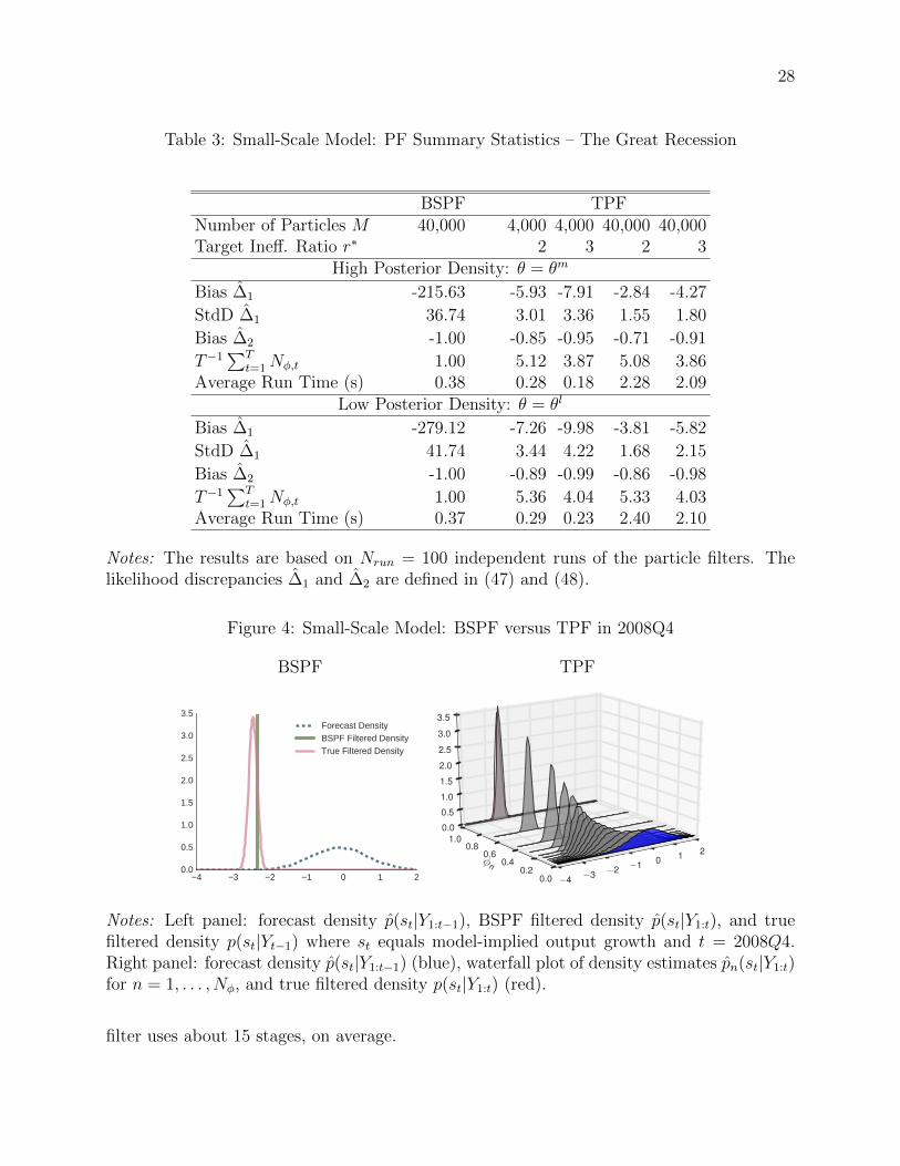
Table 3: Small-Scale Model: PF Summary Statistics – The Great Recession
BSPF TPFNumber of Particles M 40,000 4,000 4,000 40,000 40,000Target Ineff. Ratio r∗ 2 3 2 3
High Posterior Density: θ = θm
Bias ∆1 -215.63 -5.93 -7.91 -2.84 -4.27
StdD ∆1 36.74 3.01 3.36 1.55 1.80
Bias ∆2 -1.00 -0.85 -0.95 -0.71 -0.91
T−1∑T
t=1Nφ,t 1.00 5.12 3.87 5.08 3.86Average Run Time (s) 0.38 0.28 0.18 2.28 2.09
Low Posterior Density: θ = θl
Bias ∆1 -279.12 -7.26 -9.98 -3.81 -5.82
StdD ∆1 41.74 3.44 4.22 1.68 2.15
Bias ∆2 -1.00 -0.89 -0.99 -0.86 -0.98
T−1∑T
t=1Nφ,t 1.00 5.36 4.04 5.33 4.03Average Run Time (s) 0.37 0.29 0.23 2.40 2.10
Notes: The results are based on Nrun = 100 independent runs of the particle filters. Thelikelihood discrepancies ∆1 and ∆2 are defined in (47) and (48).
Figure 4: Small-Scale Model: BSPF versus TPF in 2008Q4
BSPF TPF
4 3 2 1 0 1 20.0
0.5
1.0
1.5
2.0
2.5
3.0
3.5Forecast DensityBSPF Filtered DensityTrue Filtered Density
−4 −3 −2 −1 0 1 2φn
0.00.2
0.40.6
0.81.0
0.0
0.5
1.0
1.5
2.0
2.5
3.0
3.5
Notes: Left panel: forecast density p(st|Y1:t−1), BSPF filtered density p(st|Y1:t), and truefiltered density p(st|Yt−1) where st equals model-implied output growth and t = 2008Q4.Right panel: forecast density p(st|Y1:t−1) (blue), waterfall plot of density estimates pn(st|Y1:t)for n = 1, . . . , Nφ, and true filtered density p(st|Y1:t) (red).
filter uses about 15 stages, on average.

29
Figure 4 provides an illustration of why the TPF provides much more accurate approxima-
tions than the BSPF. We focus on one particular state, namely model-implied output growth,
which is observed output growth minus its measurement error. We focus on t = 2008Q4. The
left panel depicts the BSPF approximations p(st|Y1:t−1) and p(st|Y1:t) as well as the “true”
density p(st|Y1:t). The BSPF essentially generates draws from the forecast density p(st|Y1:t−1)
and reweights them to approximate the density p(st|Y1:t). In 2008Q4, these densities have
very little overlap. This implies that essentially one draw from the forecast density receives
all the weight and the BSPF filtered density is a point mass. This point mass provides a
poor approximation of p(st|Y1:t).
The right panel of Figure 4 displays a waterfall plot of density estimates pn(st|Y1:t) for
n = 1, . . . , Nφ = 15. The densities are placed on the y-axis at the corresponding value of
φn. The first iteration in the tempering phase has φ1 = 0.002951, which corresponds to an
inflation of the measurement error variance by a factor over 300. This density looks similar
to the predictive distribution p(st|Y1:t−1), with a 1-step-ahead prediction for output growth
of about −1% (in quarterly terms). As we move through the iterations, φn increases slowly
at first and pn(st|Y1:t) gradually adds more density where st ≈ −2.5. Each correction step of
Algorithm 2 requires only modest reweighting of the particles and the mutation steps refresh
the particle values. The filter begins to tolerate relatively large changes from φn to φn+1,
as more particles lie in this region, needing only three stages to move from φn ≈ 0.29 to
φN = 1. Alongside pNφ(st|Y1:t) we also show the true filtered density in red, obtained from
the Kalman filter recursions. The TPF approximation at n = Nφ matches the true density
extremely well.
4.2 The Smets-Wouters Model
We next assess the performance of the tempered particle filter for the Smets and Wouters
(2007), henceforth SW, model. This model forms the core of the latest vintage of DSGE
models. While we leave the details of the model to the Online Appendix, it is important
to note that the SW model is estimated over the period 1966Q1 to 2004Q4 using seven
observables: the real per capita growth rates of output, consumption, investment, wages;
hours worked, inflation, and the federal funds rate. Moreover, the SW model has a high-
dimensional state space st with more than a dozen state variables. The performance of the
BSPF deteriorates quickly due to the increased state space and the fact that it is much more
difficult to predict seven observables than it is to predict three observables with a DSGE

30
Table 4: SW Model: Parameter Values
θm θl θm θl
β 0.159 0.182 π 0.774 0.571l −1.078 0.019 α 0.181 0.230σ 1.016 1.166 Φ 1.342 1.455ϕ 6.625 4.065 h 0.597 0.511ξw 0.752 0.647 σl 2.736 1.217ξp 0.861 0.807 ιw 0.259 0.452ιp 0.463 0.494 ψ 0.837 0.828rπ 1.769 1.827 ρ 0.855 0.836ry 0.090 0.069 r∆y 0.168 0.156ρa 0.982 0.962 ρb 0.868 0.849ρg 0.962 0.947 ρi 0.702 0.723ρr 0.414 0.497 ρp 0.782 0.831ρw 0.971 0.968 ρga 0.450 0.565µp 0.673 0.741 µw 0.892 0.871σa 0.375 0.418 σb 0.073 0.075σg 0.428 0.444 σi 0.350 0.358σr 0.144 0.131 σp 0.101 0.117σw 0.311 0.382 ln p(Y |θ) −943.0 −956.1
Notes: β = 100(β−1 − 1).
model. As a consequence, the estimation of nonlinear variants of the SW model has proven
extremely difficult.
We compute the particle filter approximations conditional on two sets of parameter val-
ues, θm and θl, which are summarized in Table 4. θm is the parameter vector associated with
the highest likelihood value among the draws that we generated with a posterior sampler.
θl is a parameter vector that attains a lower likelihood value. The log-likelihood difference
between the two parameter vectors is approximately 13. The standard deviations of the
measurement errors are chosen to be approximately 20% of the sample standard deviation
of the time series.10 For comparison purposes, the parameter values and the data are iden-
tical to the ones used in Chapter 8 of Herbst and Schorfheide (2015). We run each filter
Nrun = 100 times.
Figure 5 displays density estimates of the approximation errors associated with the log
10The standard deviations for the measurement errors are: 0.1731 (output growth), 0.1394 (consumptiongrowth), 0.4515 (investment growth), 0.1128 (wage growth), 0.5838 (log hours), 0.1230 (inflation), 0.1653(interest rates).

31
Figure 5: Smets-Wouters Model: Distribution of Log-Likelihood Approximation Errors
θ = θm θ = θl
−700 −600 −500 −400 −300 −200 −100 0 1000.000
0.002
0.004
0.006
0.008
0.010
0.012
0.014
0.016
0.018
Den
sity
TPF (r ∗ = 2), M = 40000
TPF (r ∗ = 2), M = 4000
TPF (r ∗ = 3), M = 40000
TPF (r ∗ = 3), M = 4000
BSPF , M = 40000
−600 −500 −400 −300 −200 −100 0 100 2000.000
0.002
0.004
0.006
0.008
0.010
0.012
0.014
0.016
Den
sity
TPF (r ∗ = 2), M = 40000
TPF (r ∗ = 2), M = 4000
TPF (r ∗ = 3), M = 40000
TPF (r ∗ = 3), M = 4000
BSPF , M = 40000
Notes: Density estimate of ∆1 = ln p(Y1:T |θm) − ln p(Y1:T |θm) based on Nrun = 100 runs ofthe particle filters.
likelihood estimates under θ = θm and θ = θl. We use M = 40, 000 particles for the BSPF.
For the TPF we use M = 4, 000 or M = 40, 000 and consider r∗ = 2 and r∗ = 3. Moreover,
in the mutation step (Algorithm 3) we set NMH = 1 and c∗ = 0.3. Under both parameter
values, the BSPF exhibits the most bias, with its likelihood estimates substantially below
the true likelihood value. The distribution of the bias falls mainly between -400 and -100.
This means that eliciting the posterior distribution of the SW model using, for example, a
particle Markov chain Monte Carlo algorithm with likelihood estimates from the bootstrap
particle filter would be nearly impossible. The TPFs perform better, although they also
underestimate the likelihood by a large amount.
Table 5 underscores the results in Figure 5. The best-performing TPF, while three to four
times more accurate than the BSPF, still generates a bias in the log-likelihood approximation
of about −55 and a standard deviation of about 21 for θ = θm. Moreover, this increased
performance comes at a cost: the TPF (r∗ = 2),M = 40, 000 filter takes about 29 seconds,
while the BSPF takes only 4 seconds. Even the variants of the TPF, which run more quickly
than the BSPF, still have wildly imprecise estimates of the likelihood; though, to be sure,
these estimates are in general better than those of the BSPF.
It is well known that in sequential Monte Carlo algorithms for static parameters the
mutation phase is crucial. For example, Bognanni and Herbst (2015) show that tailoring
the mutation step to model can substantially improve performance. The modification of the
mutation step is not immediately obvious. One clear way to allow the particles to better

32
Table 5: SW Model: PF Summary Statistics
BSPF TPFNumber of Particles M 40,000 4,000 4,000 40,000 40,000Target Ineff. Ratio r∗ 2 3 2 3
High Posterior Density: θ = θm
Bias ∆1 -235.50 -126.09 -144.57 -55.71 -65.94
StdD ∆1 60.30 46.55 44.32 20.73 23.81
Bias ∆2 -1.00 -1.00 -1.00 -1.00 -1.00
T−1∑T
t=1Nφ,t 1.00 6.19 4.75 6.14 4.71Average Run Time (s) 4.28 2.75 2.11 28.83 22.40
Low Posterior Density: θ = θl
Bias ∆1 -263.31 -138.69 -168.76 -66.92 -83.08
StdD ∆1 78.14 48.18 50.15 24.26 29.14
Bias ∆2 -1.00 -1.00 -1.00 -1.00 -1.00
T−1∑T
t=1Nφ,t 1.00 6.25 4.81 6.21 4.78Average Run Time (s) 4.17 2.34 2.16 26.01 20.14
Notes: The likelihood discrepancies ∆1 and ∆2 are defined in (47) and (48). Results arebased on Nrun = 100 runs of the particle filters.
adapt to the current density is to increase the number of Metropolis-Hastings steps. While
all of the previous results are based on NMH = 1, we now consider NMH = 10. Table
6 displays the results associated with this choice for variants of the TPF, along with the
BSPF, which is unchanged the previous exercise.
The bias shrinks dramatically. For the TPF (r∗ = 2),M = 40, 000, when θ = θm, the bias
falls from about −55 to about −6, with the standard deviation of the estimator decreasing
by a factor of 6. Of course this increase in performance comes at a computational cost.
Each filter takes about three times longer than their NMH = 1 counterpart. Note that this
is less than you might expect, given the fact the number of Metropolis-Hastings steps at
each iteration has increased by 10. This reflects two things. First, the mutation phase is
easily parallelizable on a multi-core desktop computer. Second, a substantial fraction of
computational time is spent during the resampling (selection) phase, which is not affected
by increasing the number of Metropolis-Hastings steps.
33
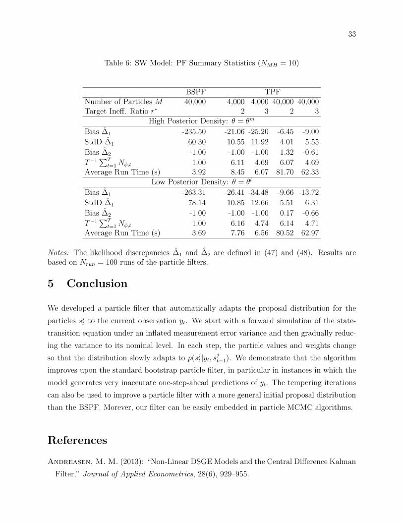
Table 6: SW Model: PF Summary Statistics (NMH = 10)
BSPF TPFNumber of Particles M 40,000 4,000 4,000 40,000 40,000Target Ineff. Ratio r∗ 2 3 2 3
High Posterior Density: θ = θm
Bias ∆1 -235.50 -21.06 -25.20 -6.45 -9.00
StdD ∆1 60.30 10.55 11.92 4.01 5.55
Bias ∆2 -1.00 -1.00 -1.00 1.32 -0.61
T−1∑T
t=1Nφ,t 1.00 6.11 4.69 6.07 4.69Average Run Time (s) 3.92 8.45 6.07 81.70 62.33
Low Posterior Density: θ = θl
Bias ∆1 -263.31 -26.41 -34.48 -9.66 -13.72
StdD ∆1 78.14 10.85 12.66 5.51 6.31
Bias ∆2 -1.00 -1.00 -1.00 0.17 -0.66
T−1∑T
t=1Nφ,t 1.00 6.16 4.74 6.14 4.71Average Run Time (s) 3.69 7.76 6.56 80.52 62.97
Notes: The likelihood discrepancies ∆1 and ∆2 are defined in (47) and (48). Results arebased on Nrun = 100 runs of the particle filters.
5 Conclusion
We developed a particle filter that automatically adapts the proposal distribution for the
particles sjt to the current observation yt. We start with a forward simulation of the state-
transition equation under an inflated measurement error variance and then gradually reduc-
ing the variance to its nominal level. In each step, the particle values and weights change
so that the distribution slowly adapts to p(sjt |yt, sjt−1). We demonstrate that the algorithm
improves upon the standard bootstrap particle filter, in particular in instances in which the
model generates very inaccurate one-step-ahead predictions of yt. The tempering iterations
can also be used to improve a particle filter with a more general initial proposal distribution
than the BSPF. Morever, our filter can be easily embedded in particle MCMC algorithms.
References
Andreasen, M. M. (2013): “Non-Linear DSGE Models and the Central Difference Kalman
Filter,” Journal of Applied Econometrics, 28(6), 929–955.

34
Andrieu, C., A. Doucet, and R. Holenstein (2010): “Particle Markov Chain Monte
Carlo Methods,” Journal of the Royal Statistical Society Series B, 72(3), 269–342.
Arulampalam, S., S. Maskell, N. Gordon, and T. Clapp (2002): “A Tutorial on
Particle Filters for Online Nonlinear/Non-Gaussian Bayesian Tracking,” IEEE Transac-
tions on Signal Processing, 50(2), 174–188.
Bognanni, M., and E. P. Herbst (2015): “Estimating (Markov-Switching) VAR Models
without Gibbs Sampling: A Sequential Monte Carlo Approach,” FEDS, 2015(116), 154.
Cappe, O., S. J. Godsill, and E. Moulines (2007): “An Overview of Existing Methods
and Recent Advances in Sequential Monte Carlo,” Proceedings of the IEEE, 95(5), 899–
924.
Cappe, O., E. Moulines, and T. Ryden (2005): Inference in Hidden Markov Models.
Springer Verlag.
Chopin, N. (2002): “A Sequential Particle Filter for Static Models,” Biometrika, 89(3),
539–551.
(2004): “Central Limit Theorem for Sequential Monte Carlo Methods and its
Application to Bayesian Inference,” Annals of Statistics, 32(6), 2385–2411.
Creal, D. (2007): “Sequential Monte Carlo Samplers for Bayesian DSGE Models,”
Manuscript, University Chicago Booth.
(2012): “A Survey of Sequential Monte Carlo Methods for Economics and Finance,”
Econometric Reviews, 31(3), 245–296.
Del Moral, P. (2013): Mean Field Simulation for Monte Carlo Integration. Chapman &
Hall/CRC.
Doucet, A., and A. M. Johansen (2011): “A Tutorial on Particle Filtering and Smooth-
ing: Fifteen Years Later,” in Handook of Nonlinear Filtering, ed. by D. Crisan, and B. Ro-
zovsky. Oxford University Press.
Durham, G., and J. Geweke (2014): “Adaptive Sequential Posterior Simulators for
Massively Parallel Computing Environments,” in Advances in Econometrics, ed. by I. Jeli-
azkov, and D. Poirier, vol. 34, chap. 6, pp. 1–44. Emerald Group Publishing Limited.

35
Fernandez-Villaverde, J., and J. F. Rubio-Ramırez (2007): “Estimating Macroeco-
nomic Models: A Likelihood Approach,” Review of Economic Studies, 74(4), 1059–1087.
Geweke, J., and B. Frischknecht (2014): “Exact Optimization By Means of Sequen-
tially Adaptive Bayesian Learning,” Mimeo.
Gordon, N., D. Salmond, and A. F. Smith (1993): “Novel Approach to Nonlinear/Non-
Gaussian Bayesian State Estimation,” Radar and Signal Processing, IEE Proceedings F,
140(2), 107–113.
Gust, C., E. Herbst, D. Lopez-Salido, and M. E. Smith (2016): “The Empirical
Implications of the Interest-Rate Lower Bound,” Manuscript, Federal Reserve Board.
Herbst, E., and F. Schorfheide (2014): “Sequential Monte Carlo Sampling for DSGE
Models,” Journal of Applied Econometrics, 19(7), 1073–1098.
(2015): Bayesian Estimation of DSGE Models. Princeton University Press, Prince-
ton.
Kollmann, R. (2015): “Tractable Latent State Filtering for Non-Linear DSGE Models
Using a Second-Order Approximation and Pruning,” Computational Economics, 45(2),
239–260.
Liu, J. S. (2001): Monte Carlo Strategies in Scientific Computing. Springer Verlag.
Pitt, M. K., R. d. S. Silva, P. Giordani, and R. Kohn (2012): “On Some Properties
of Markov Chain Monte Carlo Simulation Methods Based on the Particle Filter,” Journal
of Econometrics, 171, 134–151.
Smets, F., and R. Wouters (2007): “Shocks and Frictions in US Business Cycles: A
Bayesian DSGE Approach,” American Economic Review, 97, 586–608.
White, H. (2001): Asymptotic Theory For Econometricians. Academic Press.
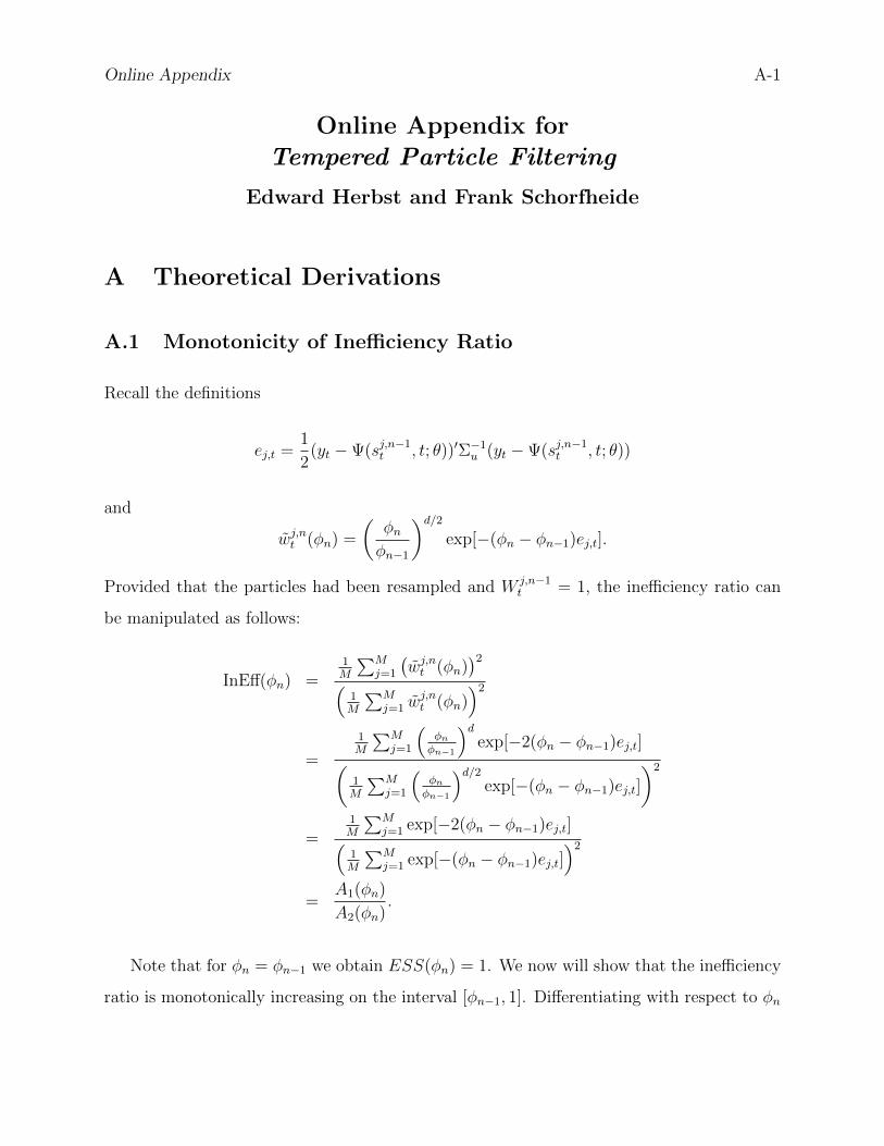
Online Appendix A-1
Online Appendix for
Tempered Particle Filtering
Edward Herbst and Frank Schorfheide
A Theoretical Derivations
A.1 Monotonicity of Inefficiency Ratio
Recall the definitions
ej,t =1
2(yt −Ψ(sj,n−1
t , t; θ))′Σ−1u (yt −Ψ(sj,n−1
t , t; θ))
and
wj,nt (φn) =
(φnφn−1
)d/2exp[−(φn − φn−1)ej,t].
Provided that the particles had been resampled and W j,n−1t = 1, the inefficiency ratio can
be manipulated as follows:
InEff(φn) =1M
∑Mj=1
(wj,nt (φn)
)2(1M
∑Mj=1 w
j,nt (φn)
)2
=
1M
∑Mj=1
(φnφn−1
)dexp[−2(φn − φn−1)ej,t](
1M
∑Mj=1
(φnφn−1
)d/2exp[−(φn − φn−1)ej,t]
)2
=1M
∑Mj=1 exp[−2(φn − φn−1)ej,t](
1M
∑Mj=1 exp[−(φn − φn−1)ej,t]
)2
=A1(φn)
A2(φn).
Note that for φn = φn−1 we obtain ESS(φn) = 1. We now will show that the inefficiency
ratio is monotonically increasing on the interval [φn−1, 1]. Differentiating with respect to φn
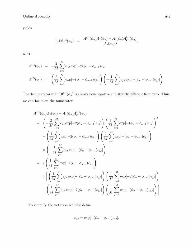
Online Appendix A-2
yields
InEff(1)(φn) =A(1)(φn)A2(φn)− A1(φn)A
(1)2 (φn)
[A2(φn)]2,
where
A(1)(φn) = − 2
M
M∑j=1
ej,t exp[−2(φn − φn−1)ej,t]
A(2)(φn) =
(2
M
M∑j=1
exp[−(φn − φn−1)ej,t]
)(− 1
M
M∑j=1
ej,t exp[−(φn − φn−1)ej,t]
).
The denumerator in InEff(1)(φn) is always non-negative and strictly different from zero. Thus,
we can focus on the numerator:
A(1)(φn)A2(φn)− A1(φn)A(1)2 (φn)
=
(− 2
M
M∑j=1
ej,t exp[−2(φn − φn−1)ej,t]
)(1
M
M∑j=1
exp[−(φn − φn−1)ej,t]
)2
−(
1
M
M∑j=1
exp[−2(φn − φn−1)ej,t]
)(2
M
M∑j=1
exp[−(φn − φn−1)ej,t]
)
×(− 1
M
M∑j=1
ej,t exp[−(φn − φn−1)ej,t]
)
= 2
(1
M
M∑j=1
exp[−(φn − φn−1)ej,t]
)
×[(
1
M
M∑j=1
ej,t exp[−(φn − φn−1)ej,t]
)(1
M
M∑j=1
exp[−2(φn − φn−1)ej,t]
)
−(
1
M
M∑j=1
ej,t exp[−2(φn − φn−1)ej,t]
)(1
M
M∑j=1
exp[−(φn − φn−1)ej,t]
)]
To simplify the notation we now define
xj,t = exp[−(φn − φn−1)ej,t].

Online Appendix A-3
Note that 0 < xj,t ≤ 1, which implies that x2j,t ≤ xj,t. Moreover, ej,t ≥ 0. We will use these
properties to establish the following bound:
A(1)(φn)A2(φn)− A1(φn)A(1)2 (φn)
= 2
(1
M
M∑j=1
xj,t
)[(1
M
M∑j=1
ej,txj,t
)(1
M
M∑j=1
x2j,t
)−(
1
M
M∑j=1
ej,tx2j,t
)(1
M
M∑j=1
xj,t
)]
≥ 2
(1
M
M∑j=1
xj,t
)[(1
M
M∑j=1
ej,txj,t
)(1
M
M∑j=1
x2j,t
)−(
1
M
M∑j=1
ej,tx2j,t
)(1
M
M∑j=1
x2j,t
)]
= 2
(1
M
M∑j=1
xj,t
)(1
M
M∑j=1
x2j,t
)[(1
M
M∑j=1
ej,txj,t
)−(
1
M
M∑j=1
ej,tx2j,t
)]≥ 0.
We conclude that the inefficiency ratio InEff(φn) in increasing in φn. �
A.2 Proofs for Section 3.1
The proofs in this section closely follow Chopin (2004) and Herbst and Schorfheide (2014).
Throughout this section we will assume that h(θ) is scalar and we use absolute values |h|instead of a general norm ‖h‖. Extensions to vector-valued h functions are straightforward.
We use C to denote a generic constant. We will make repeated use of the following moment
bound for r > 1
E[∣∣X − E[X]
∣∣r] ≤ Cr(E[∣∣X∣∣r]+
∣∣E[X]∣∣r) (A.1)
≤ 2CrE[∣∣X∣∣r],
where Cr = 1 for r = 1 and Cr = 2r−1 for r > 1. The first inequality follows from the Cr
inequality and the second inequality follows from Jensen’s inequality.
We will make use of the following SLLN (Markov, see White (2001) p. 33): Let {Zj} be
a sequence of independent random variables with finite means µj = E[Zj]. If for some δ > 0,∑∞j=1 E
[|Zj − µj|1+δ
]/j1+δ < ∞, then 1
M
∑Mj=1 Zj − µj
a.s−→ 0. Note that E[|Zj − µj|1+δ
]<
C <∞ implies that the summability condition is satisfied because∑∞
j=1(1/j)1+δ <∞.

Online Appendix A-4
Recall that under a multivariate Gaussian measurement error distribution, the density
pn(yt|st) can be bounded from above. Thus, pn(yt|st) ∈ Hnt
and ωj,nt ∈ Hnt
for any t and n.
Moreover, for any h(st, st−1) ∈ Hnt we can deduce that h(·) = h(·)ωj,nt ∈ Hn
t .
Proof of Lemma 1. (i) (30) can be established as follows. Consider the summands I and
II in (34). Recall that
I =1
M
M∑j=1
(h(sjt , s
j,Nφt−1 )− Ep(·|sjt−1)[h]
)W
j,Nφt−1 .
Conditional on the particles {sj,Nφt−1 ,Wj,Nφt−1 } the summands in term I form a triangular array
of mean-zero random variables that within each row are independently distributed. In Al-
gorithm 4 the particles were resampled during the t − 1 tempering iteration Nφ, such that
WNφt−1 = 1. Using the bound
Ep(·|st−1)
[∣∣h(st, st−1)− Ep(·|st−1)[h(st, st−1)]∣∣1+δ
]< C <∞
implied by the definition of H1t we can apply the SLLN to deduce that term I
a.s.−→ 0. The
second term in (34) takes the form
II =1
M
M∑j=1
(Ep(·|sjt−1)[h]−
∫ ∫h(st, st−1)p(st, st−1|Y1:t−1)dstdst−1
).
By assumption, Ep(·|st−1)[h] ∈ HNφt−1. The almost-sure convergence to zero of term II can now
be deduced from the recursive Assumption (29). By combining the convergence results for
terms I and II we have established (30).
(ii) The convergences in (31) and (33) follow immediately from the fact that p1(yt|st) ∈H1t . Moreover, if h(st, st−1) ∈ H1
t , then h(st, st−1)p1(yt|st) ∈ H1t . Finally, p1(yt|st) > 0,
which implies that the almost-sure limit of the denominator in (31) is strictly positive.
(iii) To verify (32), let Ft,1,M denote the σ-algebra generated by the particles {sj,1t , sj,Nφt−1 ,W
j,1t }.

Online Appendix A-5
Moreover, define
E[h|Ft,1,M ] =1
M
M∑j=1
h(sj,1t , sj,Nφt−1 )W j,1
t ,
and write
h1t,M −
∫h(st, st−1)p1(st, st−1|Y1:t)dst (A.2)
=1
M
M∑j=1
(h(sj,1t , s
j,Nφt−1 )− E[h|Ft,1,M ]
)+
(1
M
M∑j=1
h(sj,1t , sNφt−1)W j,1
t −∫ ∫
h(st, st−1)p1(st, st−1|Y1:t)dstdst−1
)
=1
M
M∑j=1
(h(sj,1t , s
j,Nφt−1 )− E[h|Ft,1,M ]
)+
(h1t,M −
∫ ∫h(st, st−1)p1(st, st−1|Y1:t)dstdst−1
)= I + II.
From (31), we can immediately deduce that term II converges to zero almost surely. Re-
call that we are resampling the pairs (sj,nt , sj,Nφt−1 ). Thus, under multinomial resampling the
h(sj,1t , sj,Nφt )’s form a triangular array of iid random variables conditional on Ft,1,M . Using
Kolmogorov’s SLLN for iid sequences, it suffices to verify for that
E[∣∣h(sj,1t , s
j,Nφt )
∣∣ ∣∣∣∣ Ft,1,M] <∞.We can manipulate the moment as follows
E[∣∣h(sj,1t , s
j,Nφt−1 )
∣∣ ∣∣∣∣ Ft,1,M] =1
M
M∑j=1
∣∣h(sj,1t , sj,Nφt−1 )
∣∣W j,1t
a.s−→∫ ∣∣h(st, st−1)
∣∣p1(st, st−1|Y1:t)dstdst−1 <∞.
Because h ∈ H1t implies |h| ∈ H1
t , we obtain the almost sure convergence from (31). �
Proof of Lemma 2. (i) We begin with the correction step. Recall that for any h(st, st−1) ∈

Online Appendix A-6
Hn−1t :
pn(yt|st)/pn−1(yt|st) ∈ Hn−1t and h(st, st−1)pn(yt|st)/pn−1(yt|st) ∈ Hn−1
t .
Thus, the recursive Assumption 2 yields the almost-sure convergence in (36) and (38).
(ii) We proceed with the selection step. The convergence in (37) can be established with
an argument similar to the one used in Step (iii) of the proof of Lemma 1.
(iii) Finally, consider the mutation step. To establish the convergence in (39) we need to
construct moment bounds for the terms I and II that appear in (41). Under the assumption
that the resampling step is executed at every iteration n, term I takes the form:
I =1
M
M∑j=1
(h(sj,nt , s
j,Nφt−1 )− E
Kn(·|sj,nt ;sj,Nφt−1 )
[h]
).
Conditional on the σ-algebra generated by the particles of the selection step, term I is an
average of independently distributed mean-zero random variables. By virtue of h ∈ Hnt , we
can deduce that, omitting the j and n superscripts,
EKn(·|st;st−1)
[∣∣h(st, st−1)− EKn(·|st;st−1)[h]∣∣1+δ]
< C <∞.
Therefore, the SLLN implies that Ia.s.−→ 0. For term II, we have
II =1
M
M∑j=1
(EKn(·|sj,nt ;s
j,Nφt−1 )
[h]−∫ ∫
h(st, st−1)pn(st, st−1|Y1:t)dstdst−1
).
Now define
ψ(st, st−1) = EKn(·|st;st−1)[h].
The definition of Hnt implies that ψ(st, st−1) ∈ Hn−1
t . Thus, we can deduce from (37) that
IIa.s.−→ 0. �

Online Appendix A-7
A.3 Proofs for Section 3.2
The subsequent proof of the unbiasedness of the particle filter approximation utilizes Lem-
mas 3 and 5 below. Throughout this section, we use the convention that W j,0t = W
j,Nφt−1 .
Moreover, we often use the j subscript to denote a fixed particle as well as a running index
in a summation. That is, we write aj/∑M
j=1 aj instead of aj/
∑Ml=1 a
l. We also define the
information set
Ft−1,n,M ={
(sj,Nφ0 ,W
j,Nφ0 ), (sj,11 ,W j,1
1 ), . . . , (sj,Nφ1 ,W
j,Nφ1 ), . . . , (A.3)
(sj,1t−1,Wj,1t−1), . . . , (sj,nt−1,W
j,nt−1)}Mj=1.
A.3.1 Additional Lemmas
Lemma 3 Suppose that the incremental weights wj,nt are defined as in (7) and (14) and that
there is no resampling. Then
Nφ∏n=1
(1
M
M∑j=1
wj,nT W j,n−1T
)=
1
M
M∑j=1
Nφ∏n=1
wj,nT
Wj,NφT−1 (A.4)
and
Wj,NφT−h−1
Nφ∏n=1
(1
M
M∑j=1
wj,nT−h−1Wj,n−1T−h−1
)=
Nφ∏n=1
wj,nT−h−1
Wj,NφT−h−2. (A.5)
Proof of Lemma 3. The lemma can be proved by induction. If there is no resampling,
then W j,nt = W j,n
t .
Part 1. The inductive hypothesis to show (A.4) takes the form
Nφ∏n=n∗
(1
M
M∑j=1
wj,nT W j,n−1T
)=
1
M
M∑j=1
Nφ∏n=n∗
wj,nT
W j,n∗−1T . (A.6)

Online Appendix A-8
If the hypothesis is correct, then
Nφ∏n=n∗−1
(1
M
M∑j=1
wj,nT W j,n−1T
)(A.7)
=
1
M
M∑j=1
Nφ∏n=n∗
wj,nT
W j,n∗−1T
( 1
M
M∑j=1
wj,n∗−1T W j,n∗−2
T
)
=
1
M
M∑j=1
Nφ∏n=n∗
wj,nT
wj,n∗−1T W j,n∗−2
T
1M
∑Mj=1 w
j,n∗−1T W j,n∗−2
T
( 1
M
M∑j=1
wj,n∗−1T W j,n∗−2
T
)
=1
M
M∑j=1
Nφ∏n=n∗−1
wj,nT
W j,n∗−2T .
The first equality follows from (A.6) and the second equality is obtained by using the defi-
nition of W j,n∗−1T .
It is straightforward to verify that the inductive hypothesis (A.6) is satisfied for n∗ = Nφ.
Setting n∗ = 1 in (A.6) and noticing that W j,0T = W
j,NφT−1 leads the desired result.
Part 2. To show (A.5), we can use the inductive hypothesis
Wj,NφT−h−1
Nφ∏n=n∗
(1
M
M∑j=1
wj,nT−h−1Wj,n−1T−h−1
)=
Nφ∏n=n∗
wj,nT−h−1
W j,n∗−1T−h−1. (A.8)
If the inductive hypothesis is satisfied, then
Wj,NφT−h−1
Nφ∏n=n∗−1
(1
M
M∑j=1
wj,nT−h−1Wj,n−1T−h−1
)(A.9)
= Wj,NφT−h−1
Nφ∏n=n∗
(1
M
M∑j=1
wj,nT−h−1Wj,n−1T−h−1
)(1
M
M∑j=1
wj,n∗−1T−h−1W
j,n∗−2T−h−1
)
=
Nφ∏n=n∗
wj,nT−h−1
wj,n∗−1T−h−1W
j,n∗−2T−h−1
1M
∑Mj=1 w
j,n∗−1T−h−1W
j,n∗−2T−h−1
(1
M
M∑j=1
wj,n∗−1T−h−1W
j,n∗−2T−h−1
)
=
Nφ∏n=n∗−1
wj,nT−h−1
W j,n∗−2T−h−1.

Online Appendix A-9
For n∗ = Nφ the validity of the inductive hypothesis can be verified as follows:
Wj,NφT−h−1
(1
M
M∑j=1
wj,NφT−h−1W
j,Nφ−1
T−h−1
)(A.10)
=wj,NφT−h−1W
j,Nφ−1
T−h−1
1M
∑Mj=1 w
j,NφT−h−1W
j,Nφ−1
T−h−1
(1
M
M∑j=1
wj,NφT−h−1W
j,Nφ−1
T−h−1
)= w
j,NφT−h−1W
j,Nφ−1
T−h−1 .
Setting n∗ = 1 in (A.8) leads to the desired result. �
The following lemma simply states that the expected value of a sum is the sum of the
expected values, but it does so using a notation that we will encounter below.
Lemma 4 Suppose sj, j = 1, . . . ,M , is a sequence of random variables with density∏M
j=1 p(sj),
then
∫· · ·∫ (
1
M
M∑j=1
f(sj)
)( M∏j=1
p(sj)
)ds1 · · · dsM =
1
M
M∑j=1
∫f(sj)p(sj)dsj.
Proof of Lemma 4. The statement is trivially satisfied for M = 1. Suppose that it is true
for M − 1, then
∫· · ·∫ (
1
M
M∑j=1
f(sj)
)( M∏j=1
p(sj)
)ds1 · · · dsM (A.11)
=
∫· · ·∫ (
1
Mf(sM) +
M − 1
M
1
M − 1
M−1∑j=1
f(sj)
)(p(sM)
M−1∏j=1
p(sj)
)ds1 · · · dsM
=
(1
M
∫f(sM)p(sM)dsM
)M−1∏j=1
∫p(sj)dsj
+
(M − 1
M
1
M − 1
M−1∑j=1
∫f(sj)p(sj)dsj
)∫p(sM)dsM
=1
M
M∑j=1
∫f(sj)p(sj)dsj, (A.12)
which verifies the claim for all M by induction. �

Online Appendix A-10
Lemma 5 Suppose that the incremental weights wj,nt are defined as in (7) and (14) and
that the selection step is implemented by multinomial resampling for a predetermined set of
iterations n ∈ N . Then
E
Nφ∏n=1
(1
M
M∑j=1
wj,nT W j,n−1T
)∣∣∣∣FT−1,Nφ,M
=1
M
M∑j=1
p(yT |sj,NφT−1)Wj,NφT−1 (A.13)
and
1
M
M∑j=1
E
p(YT−h:T |sj,NφT−h−1)Wj,NφT−h−1
Nφ∏n=1
(1
M
M∑j=1
wj,nT−h−1Wj,n−1T−h−1
)∣∣∣∣FT−h−2,Nφ,M
(A.14)
=1
M
M∑j=1
p(YT−h−1:T |sj,NφT−h−2)Wj,NφT−h−2.
Proof of Lemma 5. We first prove the Lemma under the assumption of no resampling,
i.e., N = ∅. We then discuss how the proof can be modified to allow for resampling.
Part 1 (No Resampling). We deduce from Lemma 3 that
E[ Nφ∏n=1
(1
M
M∑j=1
wj,nT W j,n−1T
)∣∣∣∣FT−1,Nφ,M
]=
1
M
M∑j=1
E[ Nφ∏
n=1
wj,nT
Wj,NφT−1
∣∣∣∣FT−1,Nφ,M
].
(A.15)
The subsequent derivations focus on the evaluation of the expectation on the right-hand-
side of this equation. We will subsequently integrate over the particles s1:M,1T , . . . , s
1:M,Nφ−1T ,
which enter the incremental weights wj,nT . We use s1:M,nT to denote the set of particle values
{s1,nT , . . . , sM,n
T }. Because Wj,NφT−1 ∈ FT−1,Nφ,M it suffices to show that
E[ Nφ∏
n=1
wj,nT
∣∣∣∣FT−1,Nφ,M
]= p(yT |sj,NφT−1). (A.16)
Recall that the initial state particle sj,1T is generated from the state-transition equation

Online Appendix A-11
p(sT |sj,NφT−1). The first incremental weight is defined as
wj,1T = p1(yT |sj,1T ).
The incremental weight in tempering iteration n is given by
wj,nT =pn(yT |sj,n−1
T )
pn−1(yT |sj,n−1T )
.
Because we are omitting the selection step, the new particle value is generated in the mutation
step by sampling from the Markov transition kernel
sj,nT ∼ Kn(snT |sj,n−1T , s
j,NφT−1), (A.17)
which has the invariance property
pn(sT |yT , sT−1) =
∫Kn(sT |sT ; sT−1)pn(sT |yT , sT−1)dsT . (A.18)
Using the above notation, we can write
E
Nφ∏n=1
wj,nT
∣∣∣∣FT−1,Nφ,M
(A.19)
=
∫· · ·∫ Nφ∏
n=3
pn(yT |sj,n−1T )
pn−1(yT |sj,n−1T )
Kn−1(sj,n−1T |sj,n−2
T , sj,NφT−1)
×p2(yT |sj,1T )
p1(yT |sj,1T )p1(yT |sj,1T )p(sj,1T |s
j,NφT−1)dsj,1T · · · ds
j,Nφ−1T .
The bridge posterior densities were defined as
pn(st|yt, st−1) =pn(yt|st)p(st|st−1)
pn(yt|st−1), pn(yt|st−1) =
∫pn(yt|st)p(st|st−1)dst. (A.20)
Using the invariance property of the transition kernel in (A.18) and the definition of the

Online Appendix A-12
bridge posterior densities, we deduce that
∫Kn−1(sj,n−1
T |sj,n−2T , s
j,NφT−1)pn−1(yT |sj,n−2
T )p(sj,n−2T |sj,NφT−1)dsj,n−2
T (A.21)
=
∫Kn−1(sj,n−1
T |sj,n−2T , s
j,NφT−1)pn−1(sj,n−2
T |yT , sj,NφT−1)pn−1(yT |sj,NφT−1)dsj,n−2T
= pn−1(sj,n−1T |yT , sj,NφT−1)pn−1(yT |sj,NφT−1)
= pn−1(yT |sj,n−1T )p(sj,n−1
T |sj,NφT−1).
The first equality follows from Bayes Theorem in (A.20). The second equality follows from
the invariance property of the transition kernel. The third equality uses Bayes Theorem
again.
We can now evaluate the integrals in (A.19). Consider the terms involving sj,1T∫K2(sj,2T |sj,1T , s
j,NφT−1)
p2(yT |sj,1T )
p1(yT |sj,1T )p1(yT |sj,1T )p(sj,1T |s
j,NφT−1)dsj,1T (A.22)
=
∫K2(sj,2T |sj,1T , s
j,NφT−1)p2(yT |sj,1T )p(sj,1T |s
j,NφT−1)dsj,1T
= p2(yT |sj,2T )p(sj,2T |sj,NφT−1).
Thus,
E
Nφ∏n=1
wj,nT
∣∣∣∣FT−1,Nφ,M
(A.23)
=
∫· · ·∫ Nφ∏
n=4
pn(yT |sj,n−1T )
pn−1(yT |sj,n−1T )
Kn−1(sj,n−1T |sj,n−2
T , sj,NφT−1)
×p3(yT |sj,2T )
p2(yT |sj,2T )p2(yT |sj,2T )p(sj,2T |s
j,NφT−1)dsj,2T · · · ds
j,Nφ−1T
=
∫pNφ(yT |sj,Nφ−1
T )
pNφ−1(yT |sj,Nφ−1T )
pNφ−1(yT |sj,Nφ−1T )p(s
j,Nφ−1T |sj,NφT−1)ds
j,Nφ−1T
= p(yT |sj,NφT−1).
The first equality follows from (A.22). The second equality is obtained by sequentially
integrating out sj,2T , . . . , sj,Nφ−2
T , using a similar argument as for sj,1T . This proves the first

Online Appendix A-13
part of the Lemma.
Part 2 (No Resampling). Using Lemma 3 we write
E[p(YT−h:T |sj,NφT−h−1, θ)W
j,NφT−h−1
Nφ∏n=1
(1
M
M∑j=1
wj,nT−h−1Wj,n−1T−h−1
)∣∣∣∣FT−h−2,Nφ,M
]
= E[p(YT−h:T |sj,NφT−h−1, θ)
Nφ∏n=1
wj,nT−h−1
Wj,NφT−h−2
∣∣∣∣FT−h−2,Nφ,M
](A.24)
To prove the second part of the Lemma we slightly modify the last step of the integration
in (A.23):
E
p(YT−h:T |sj,NφT−h−1)
Nφ∏n=1
wj,nT−h−1
∣∣∣∣FT−2,Nφ,M
(A.25)
=
∫p(YT−h:T |sj,NφT−h−1)pNφ(yT−h−1|sj,Nφ−1
T−h−1)p(sj,Nφ−1
T−h−1|sj,NφT−h−2)ds
j,Nφ−1
T−h−1
= p(YT−h−1:T |sj,NφT−h−2),
as required.
Part 1 (Resampling in tempering iteration n). We now assume that the selection step is
executed once, in iteration n, i.e., N = {n}. For reasons that will become apparent subse-
quently, we will use i subscripts for particles in stages n = 1, . . . , n− 1. Using Lemma 3, we
deduce that it suffices to show:
E[( n−1∏
n=1
(1
M
M∑i=1
wi,nT W i,n−1T
))(1
M
M∑j=1
wj,nT W j,n−1T
)(A.26)
×(
1
M
M∑j=1
( Nφ∏n=n+1
wj,nT
)W j,nT
)∣∣∣∣FT−1,Nφ,M
]
=1
M
M∑j=1
p(yT |sj,NφT−1)Wj,NφT−1 .
To evaluate the expectation, we need to integrate over the particles s1:M,1T , . . . , s
1:M,NφT as well

Online Appendix A-14
as the particles s1:M,nT generated during the selection step. We have to distinguish two cases:
Case 1, n 6= n : sj,nT ∼ Kn(sj,nT |sj,n−1T , s
j,NφT ), j = 1, . . . ,M
Case 2, n = n : sj,nT ∼ Kn(sj,nT |sj,nT , sj,NφT ), j = 1, . . . ,M ;
sj,nT ∼MN(s1:M,n−1T , W 1:M,n
T
), j = 1, . . . ,M
where MN(·) here denotes the multinomial distribution.
In a preliminary step, we are integrating out the particles s1:M,nT . These particles enter the
Markov transition kernel Kn(sj,nT |sj,nT , sj,NφT−1) as well as the conditional density p(sj,nT |s1:M,n−1
T ).
Under the assumption that the resampling step is executed using multinomial resampling,
p(sj,nT |s1:M,n−1T ) =
1
M
M∑i=1
W j,nT δ(sj,nT − si,n−1
T ),
where δ(x) is the Dirac function with the property that δ(x) = 0 for x 6= 0 and∫δ(x)dx = 1.
Integrating out the resampled particles yields
p(s1:M,nT |s1:M,n−1
T ) (A.27)
=
∫ M∏j=1
Kn(sj,nT |sj,nT , sj,NφT−1)
[1
M
M∑i=1
W i,nT δ(sj,nT − si,n−1
T )
]ds1:M,n
T
=M∏j=1
∫Kn(sj,nT |sj,nT , s
j,NφT−1)
[1
M
M∑i=1
W i,nT δ(sj,nT − si,n−1
T )
]dsj,nT
=M∏j=1
[1
M
M∑i=1
W i,nT Kn(sj,nT |si,n−1
T , si,NφT−1)
].
In the last equation, the superscript for sT−1 changes from j to i because during the resam-
pling, we keep track of the history of the particle. Thus, if for particle j = 1 the value s1,nT
is set to s3,n−1T , we also use s
3,NφT−1 for this particle.
We can now express the expected value, which we abbreviate as E , as the following

Online Appendix A-15
integral:
E = E[( n−1∏
n=1
(1
M
M∑i=1
wi,nT W i,n−1T−1
))(1
M
M∑j=1
wj,nT W j,n−1T
)(A.28)
×(
1
M
M∑j=1
( Nφ∏n=n+1
wj,nT
)W j,nT
)∣∣∣∣FT−1,Nφ,M
]
=
∫· · ·∫ ( n−1∏
n=1
(1
M
M∑i=1
wi,nT W i,n−1T−1
))(1
M
M∑j=1
wj,nT W j,n−1T
)(1
M
M∑j=1
( Nφ∏n=n+1
wj,nT
))
×( n−1∏n=1
M∏j=1
Kn(si,nT |si,n−1T , s
i,NφT−1)
)( M∏j=1
[1
M
M∑i=1
W i,nT Kn(sj,nT |si,n−1
T , si,NφT−1)
])
×( Nφ−1∏n=n+1
M∏j=1
Kn(sj,nT |sj,n−1T , s
j,NφT−1)
)ds1:M,1
T · · · ds1:M,Nφ−1T .
For the second equality we used the fact that W j,nT = 1.
Using Lemma 4, we can write
∫· · ·∫ (
1
M
M∑j=1
( Nφ∏n=n+1
wj,nT
)( Nφ−1∏n=n+1
M∏j=1
Kn(sj,nT |sj,n−1T , s
j,NφT−1)
)ds1:M,n+1
T · · · ds1:M,Nφ−1T
=1
M
M∑j=1
∫· · ·∫ ( Nφ∏
n=n+1
wj,nT
)( Nφ−1∏n=n+1
Kn(sj,nT |sj,n−1T , s
j,NφT−1)
)dsj,n+1
T · · · dsj,Nφ−1T
=1
M
M∑j=1
F (sj,nT , sj,NφT−1). (A.29)

Online Appendix A-16
Now consider the following integral involving terms that depend on s1:M,nT :
I1 =
∫ (1
M
M∑j=1
F(sj,nT , s
j,NφT−1
))( 1
M
M∑j=1
wj,nT W j,n−1T
)(A.30)
×M∏j=1
[1
M
M∑i=1
W i,nT Kn(sj,nT |si,n−1
T , si,NφT−1)
]ds1:M,n
T
=
(1
M
M∑j=1
∫F(sj,nT , s
j,NφT−1
)[ 1
M
M∑i=1
W i,nT Kn(sj,nT |si,n−1
T , si,NφT−1)
]dsj,nT
)
×(
1
M
M∑j=1
wj,nT W j,n−1T
)
=1
M
M∑j=1
∫F(sj,nT , s
j,NφT−1
)[ 1
M
M∑i=1
wi,nT W i,n−1T Kn(sj,nT |si,n−1
T , si,NφT−1)
]dsj,nT .
The first equality is the definition of I1. The second equality is a consequence of Lemma 4.
The last equality is obtained by recalling that
W i,nT =
wi,nT W i,n−1T
1M
∑Mi=1 w
i,nT W i,n−1
T
.
We proceed in the evaluation of the expected value E by integrating over the particle
values s1:M,1T , . . . , s1:M,n−1
T :
E =
∫· · ·∫I1 ·( n−1∏n=1
(1
M
M∑i=1
wi,nT W i,n−1T
))(A.31)
×( n−1∏n=1
M∏j=1
Kn(si,nT |si,n−1T , s
i,NφT−1)
)ds1:M,1
T · · · ds1:M,n−1T ,

Online Appendix A-17
where
I1 ·( n−1∏n=1
(1
M
M∑i=1
wi,nT W i,n−1T
))
=
(1
M
M∑j=1
∫F(sj,nT , s
j,NφT−1
)[ 1
M
M∑i=1
wi,nT W i,n−1T Kn(sj,nT |si,n−1
T , si,NφT−1)
]dsj,nT
)
×( n−1∏n=1
(1
M
M∑i=1
wi,nT W i,n−1T
))
=1
M
M∑j=1
∫F(sj,nT , s
j,NφT−1
)[ 1
M
M∑i=1
wi,nT W i,n−1T
( n−1∏n=1
(1
M
M∑i=1
wi,nT W i,n−1T
))×Kn(sj,nT |si,n−1
T , si,NφT−1)
]dsj,nT
=1
M
M∑j=1
∫F(sj,nT , s
j,NφT−1
)[ 1
M
M∑i=1
wi,nT
( n−1∏n=1
wi,nT
)W
i,NφT−1
×Kn(sj,nT |si,n−1T , s
i,NφT−1)
]dsj,nT .
The last equality follows from the second part of Lemma 3. Notice the switch from j to i
superscript for functions of particles in stages n < n. Thus,
E =1
M
M∑j=1
∫F(sj,nT , s
j,NφT−1
) ∫· · ·∫ [
1
M
M∑i=1
wi,nT
( n−1∏n=1
wi,nT
)W
i,NφT−1 (A.32)
×Kn(sj,nT |si,n−1T , s
i,NφT−1)
]( n−1∏n=1
M∏i=1
Kn(si,nT |si,n−1T , s
i,NφT−1)
)ds1:M,1
T · · · ds1:M,n−1T dsj,nT
=1
M
M∑j=1
∫F(sj,nT , s
j,NφT−1
)[ 1
M
M∑i=1
∫· · ·∫ ( n∏
n=1
wi,nT
)W
i,NφT−1
×Kn(sj,nT |si,n−1T , s
i,NφT−1)
n−1∏n=1
Kn(si,nT |si,n−1T , s
i,NφT−1)dsi,1T · · · dsi,n−1
T
]dsj,nT
The second equality follows from Lemma 4. The calculations in (A.23) imply that
∫· · ·∫ ( n∏
n=1
wi,nT
)W
i,NφT−1
n−1∏n=1
Kn(si,nT |si,n−1T , s
i,NφT−1)dsi,1T · · · dsi,n−2
T (A.33)
= pn−1(yT |si,n−1T )p(si,n−1
T |si,NφT−1)Wi,NφT−1

Online Appendix A-18
In turn,
E =1
M
M∑j=1
∫F(sj,nT , s
j,NφT−1
)[ 1
M
M∑i=1
∫Kn(sj,nT |si,n−1
T , si,NφT−1)
×pn(yT |si,n−1T )p(si,n−1
T |si,NφT−1)Wi,NφT−1 ds
i,n−1T
]dsj,nT
=1
M
M∑i=1
[1
M
M∑j=1
∫F(sj,nT , s
j,NφT−1
)Kn(sj,nT |si,n−1
T , si,NφT−1)dsj,nT (A.34)
×pn(yT |si,n−1T )p(si,n−1
T |si,NφT−1)Wi,NφT−1 ds
i,n−1T
]=
1
M
M∑i=1
∫F(si,nT , s
i,NφT−1
)pn(yT |si,nT )p(si,nT |s
i,NφT−1)W
i,NφT−1 ds
i,nT
=1
M
M∑j=1
∫· · ·∫ ( Nφ∏
n=n+1
wj,nT
)( Nφ−1∏n=n+1
Kn(sj,nT |sj,n−1T , s
j,NφT−1)
)×pn(yT |sj,nT )p(sj,nT |s
j,NφT−1)W
j,NφT−1 ds
j,n+1T · · · dsj,Nφ−1
T pn(yT |sj,nT )p(sj,nT |sj,NφT−1)dsj,nT
=1
M
M∑j=1
p(yT |sj,NφT−1)Wj,NφT−1 .
The second equality is obtained by changing the order of two summations. To obtain the
third equality we integrate out the si,n−1T terms along the lines of (A.21). Notice that the
value of the integral is identical for all values of the j superscript. Thus, we simply set j = i
and drop the average. For the fourth equality, we plug in the definition of F(si,nT , s
i,NφT−1
)and
replace the i index with a j index. The last equality follows from calculations similar to
those in (A.23). This completes the analysis of Part 1.
Part 2 (Resampling in tempering iteration n). A similar argument as for Part 1 can be used
to extend the result for Part 2.
Resampling in multiple tempering iterations. The previous analysis can be extended to the
case in which the selection step is executed in multiple tempering iterations n ∈ N , assuming
that the set N does not itself depend on the particle system. �

Online Appendix A-19
A.3.2 Proof of Main Theorem
Proof of Theorem 2. Suppose that for any h such that 0 ≤ h ≤ T − 1
E[p(YT−h:T |Y1:T−h−1, θ)|FT−h−1,Nφ,M
]=
1
M
M∑j=1
p(YT−h:T |sj,NφT−h−1, θ)Wj,NφT−h−1, (A.35)
where
p(YT−h:T |Y1:T−h−1, θ) =T∏
t=T−h
Nφ∏n=1
(1
M
M∑j=1
wj,nt W j,n−1t
) .
Then, by setting h = T − 1, we can deduce that
E[p(Y1:T |θ)|F0,Nφ,M
]=
1
M
M∑j=1
p(Y1:T |sj,Nφ0 , θ)Wj,Nφ0 . (A.36)
Recall that for period t = 0 we adopted the convention that Nφ = 1 and assumed that the
states were initialized by direct sampling: sj,Nφ0 ∼ p(s0) and W
j,Nφ0 = 1. Thus,
E[p(Y1:T |θ)
]= E
[E[p(Y1:T |θ)|F0,Nφ,M
]](A.37)
= E[
1
M
M∑j=1
p(Y1:T |sj,Nφ0 , θ)Wj,Nφ0
]=
∫p(Y1:T |s0, θ)p(s0)ds0
= p(Y1:T |θ),
as desired.
In the remainder of the proof we use an inductive argument to establish (A.35). If (A.35)

Online Appendix A-20
holds for h, it also has to hold for h+ 1:
E[p(YT−h−1:T |Y1:T−h−2, θ)|FT−h−2,Nφ,M
]= E
[E[p(YT−h:T |Y1:T−h−1, θ)
∣∣FT−h−1,Nφ,M
]p(yT−h−1|Y1:T−h−2, θ)
∣∣∣∣FT−h−2,Nφ,M
]=
1
M
M∑j=1
E[p(YT−h:T |sj,NφT−h−1, θ)W
j,NφT−h−1p(yT−h−1|Y1:T−h−2, θ)
∣∣FT−h−2,Nφ,M
]=
1
M
M∑j=1
E
p(YT−h:T |sj,NφT−h−1, θ)Wj,NφT−h−1
Nφ∏n=1
(1
M
M∑j=1
wj,nT−h−1Wj,n−1T−h−1
)∣∣∣∣FT−h−2,Nφ,M
=
1
M
M∑j=1
p(YT−h−1:T |sj,NφT−h−2, θ)Wj,NφT−h−2
Note that FT−h−2,Nφ,M ⊂ FT−h−1,Nφ,M . Thus, the first equality follows from the law of iter-
ated expectations. The second equality follows from the inductive hypothesis (A.35). The
third equality uses the definition of the period-likelihood approximation in (21) of Algo-
rithm 2. The last equality follows from the second part of Lemma 5.
We now verify that the inductive hypothesis (A.35) holds for h = 0. Using the definition
of p(yT |Y1:T−1, θ), we can write
E[p(yT |Y1:T−1, θ)|FT−1,Nφ,M
]= E
Nφ∏n=1
(1
M
M∑j=1
wj,nT W j,n−1T
)∣∣∣∣FT−1,Nφ,M
(A.38)
=1
M
M∑j=1
p(yT |sj,NφT−1)Wj,NφT−1 .
The second equality follows from the first part of Lemma 5. Thus, we can deduce that (A.35)
holds for h = T − 1 as required. This completes the proof. �
B Computational Details
The code for this project is available at http://github.com/eph/tempered_pf. The appli-
cations in Section 4 were coded in Fortran and compiled using the Intel Fortran Compiler

Online Appendix A-21
(version: 13.0.0), including the math kernel library. The calculations in Algorithm 1, part
2(a)ii, Algorithm 2, part 1(a)i, and Algorithm 2, part 2(c) were implemented using OpenMP
(shared memory) multithreading.
C DSGE Models and Data Sources
C.1 Small-Scale DSGE Model
C.1.1 Equilibrium Conditions
We write the equilibrium conditions by expressing each variable in terms of percentage
deviations from its steady state value. Let xt = ln(xt/x) and write
1 = βEt[e−τ ct+1+τ ct+Rt−zt+1−πt+1
](A.39)
0 =(eπt − 1
) [(1− 1
2ν
)eπt +
1
2ν
](A.40)
−βEt[(eπt+1 − 1
)e−τ ct+1+τ ct+yt+1−yt+πt+1
]+
1− ννφπ2
(1− eτ ct
)ect−yt = e−gt − φπ2g
2
(eπt − 1
)2(A.41)
Rt = ρRRt−1 + (1− ρR)ψ1πt (A.42)
+(1− ρR)ψ2 (yt − gt) + εR,t
gt = ρggt−1 + εg,t (A.43)
zt = ρz zt−1 + εz,t. (A.44)
Log-linearization and straightforward manipulation of Equations (A.39) to (A.41) yield
the following representation for the consumption Euler equation, the New Keynesian Phillips

Online Appendix A-22
curve, and the monetary policy rule:
yt = Et[yt+1]− 1
τ
(Rt − Et[πt+1]− Et[zt+1]
)(A.45)
+gt − Et[gt+1]
πt = βEt[πt+1] + κ(yt − gt)
Rt = ρRRt−1 + (1− ρR)ψ1πt + (1− ρR)ψ2 (yt − gt) + εR,t
where
κ = τ1− ννπ2φ
. (A.46)
In order to construct a likelihood function, we have to relate the model variables to a set
of observables yt. We use the following three observables for estimation: quarter-to-quarter
per capita GDP growth rates (YGR), annualized quarter-to-quarter inflation rates (INFL),
and annualized nominal interest rates (INT). The three series are measured in percentages
and their relationship to the model variables is given by the following set of equations:
Y GRt = γ(Q) + 100(yt − yt−1 + zt) (A.47)
INFLt = π(A) + 400πt
INTt = π(A) + r(A) + 4γ(Q) + 400Rt.
The parameters γ(Q), π(A), and r(A) are related to the steady states of the model economy
as follows:
γ = 1 +γ(Q)
100, β =
1
1 + r(A)/400, π = 1 +
π(A)
400.
The structural parameters are collected in the vector θ. Since in the first-order approximation
the parameters ν and φ are not separately identifiable, we express the model in terms of κ,
defined in (A.46). Let
θ = [τ, κ, ψ1, ψ2, ρR, ρg, ρz, r(A), π(A), γ(Q), σR, σg, σz]
′.

Online Appendix A-23
C.1.2 Data Sources
1. Per Capita Real Output Growth Take the level of real gross domestic product,
(FRED mnemonic “GDPC1”), call it GDPt. Take the quarterly average of the Civilian
Non-institutional Population (FRED mnemonic “CNP16OV” / BLS series “LNS10000000”),
call it POPt. Then,
Per Capita Real Output Growth
= 100
[ln
(GDPtPOPt
)− ln
(GDPt−1
POPt−1
)].
2. Annualized Inflation. Take the CPI price level, (FRED mnemonic “CPIAUCSL”),
call it CPIt. Then,
Annualized Inflation = 400 ln
(CPItCPIt−1
).
3. Federal Funds Rate. Take the effective federal funds rate (FRED mnemonic “FED-
FUNDS”), call it FFRt. Then,
Federal Funds Rate = FFRt.
C.2 The Smets-Wouters Model
C.2.1 Equilibrium Conditions
The log-linearized equilibrium conditions of the Smets and Wouters (2007) model take the
following form:

Online Appendix A-24
yt = cy ct + iy it + zyzt + εgt (A.48)
ct =h/γ
1 + h/γct−1 +
1
1 + h/γEtct+1 (A.49)
+wlc(σc − 1)
σc(1 + h/γ)(lt − Etlt+1)
− 1− h/γ(1 + h/γ)σc
(rt − Etπt+1)− 1− h/γ(1 + h/γ)σc
εbt
it =1
1 + βγ(1−σc)it−1 +
βγ(1−σc)
1 + βγ(1−σc)Etit+1 (A.50)
+1
ϕγ2(1 + βγ(1−σc))qt + εit
qt = β(1− δ)γ−σcEtqt+1 − rt + Etπt+1 (A.51)
+(1− β(1− δ)γ−σc)Etrkt+1 − εbtyt = Φ(αkst + (1− α)lt + εat ) (A.52)
kst = kt−1 + zt (A.53)
zt =1− ψψ
rkt (A.54)
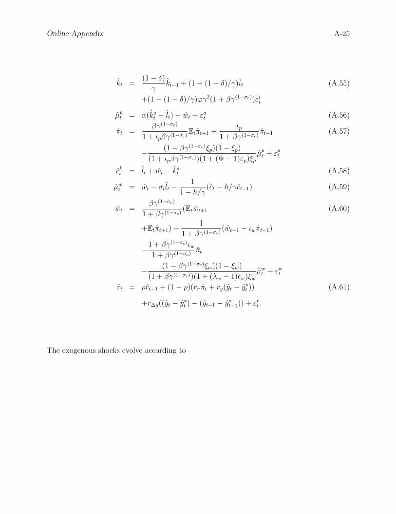
Online Appendix A-25
kt =(1− δ)γ
kt−1 + (1− (1− δ)/γ)it (A.55)
+(1− (1− δ)/γ)ϕγ2(1 + βγ(1−σc))εit
µpt = α(kst − lt)− wt + εat (A.56)
πt =βγ(1−σc)
1 + ιpβγ(1−σc)Etπt+1 +
ιp1 + βγ(1−σc)
πt−1 (A.57)
− (1− βγ(1−σc)ξp)(1− ξp)(1 + ιpβγ(1−σc))(1 + (Φ− 1)εp)ξp
µpt + εpt
rkt = lt + wt − kst (A.58)
µwt = wt − σl lt −1
1− h/γ (ct − h/γct−1) (A.59)
wt =βγ(1−σc)
1 + βγ(1−σc)(Etwt+1 (A.60)
+Etπt+1) +1
1 + βγ(1−σc)(wt−1 − ιwπt−1)
−1 + βγ(1−σc)ιw1 + βγ(1−σc)
πt
− (1− βγ(1−σc)ξw)(1− ξw)
(1 + βγ(1−σc))(1 + (λw − 1)εw)ξwµwt + εwt
rt = ρrt−1 + (1− ρ)(rππt + ry(yt − y∗t )) (A.61)
+r∆y((yt − y∗t )− (yt−1 − y∗t−1)) + εrt .
The exogenous shocks evolve according to

Online Appendix A-26
εat = ρaεat−1 + ηat (A.62)
εbt = ρbεbt−1 + ηbt (A.63)
εgt = ρgεgt−1 + ρgaη
at + ηgt (A.64)
εit = ρiεit−1 + ηit (A.65)
εrt = ρrεrt−1 + ηrt (A.66)
εpt = ρrεpt−1 + ηpt − µpηpt−1 (A.67)
εwt = ρwεwt−1 + ηwt − µwηwt−1. (A.68)

Online Appendix A-27
The counterfactual no-rigidity prices and quantities evolve according to
y∗t = cy c∗t + iy i
∗t + zyz
∗t + εgt (A.69)
c∗t =h/γ
1 + h/γc∗t−1 +
1
1 + h/γEtc∗t+1 (A.70)
+wlc(σc − 1)
σc(1 + h/γ)(l∗t − Etl∗t+1)
− 1− h/γ(1 + h/γ)σc
r∗t −1− h/γ
(1 + h/γ)σcεbt
i∗t =1
1 + βγ(1−σc)i∗t−1 +
βγ(1−σc)
1 + βγ(1−σc)Eti∗t+1
+1
ϕγ2(1 + βγ(1−σc))q∗t + εit (A.71)
q∗t = β(1− δ)γ−σcEtq∗t+1 − r∗t (A.72)
+(1− β(1− δ)γ−σc)Etrk∗t+1 − εbty∗t = Φ(αks∗t + (1− α)l∗t + εat ) (A.73)
ks∗t = k∗t−1 + z∗t (A.74)
z∗t =1− ψψ
rk∗t (A.75)
k∗t =(1− δ)γ
k∗t−1 + (1− (1− δ)/γ)it (A.76)
+(1− (1− δ)/γ)ϕγ2(1 + βγ(1−σc))εit
w∗t = α(ks∗t − l∗t ) + εat (A.77)
rk∗t = l∗t + w∗t − k∗t (A.78)
w∗t = σl l∗t +
1
1− h/γ (c∗t + h/γc∗t−1). (A.79)
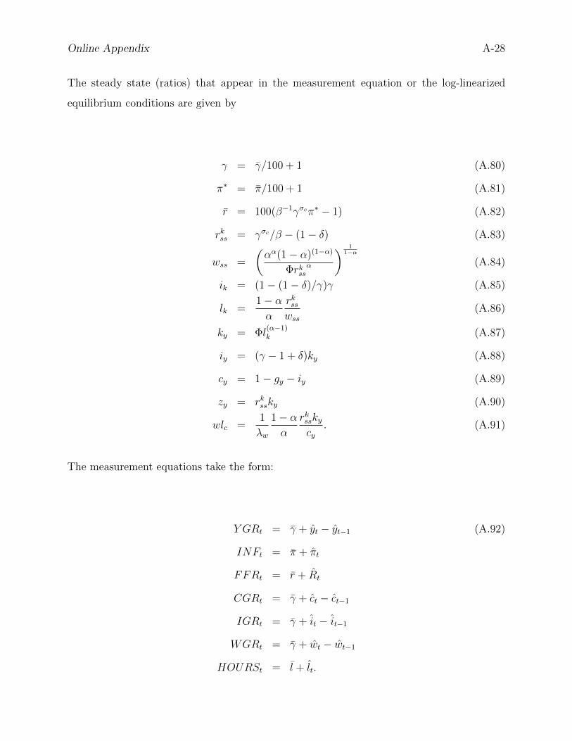
Online Appendix A-28
The steady state (ratios) that appear in the measurement equation or the log-linearized
equilibrium conditions are given by
γ = γ/100 + 1 (A.80)
π∗ = π/100 + 1 (A.81)
r = 100(β−1γσcπ∗ − 1) (A.82)
rkss = γσc/β − (1− δ) (A.83)
wss =
(αα(1− α)(1−α)
Φrkssα
) 11−α
(A.84)
ik = (1− (1− δ)/γ)γ (A.85)
lk =1− αα
rksswss
(A.86)
ky = Φl(α−1)k (A.87)
iy = (γ − 1 + δ)ky (A.88)
cy = 1− gy − iy (A.89)
zy = rkssky (A.90)
wlc =1
λw
1− αα
rksskycy
. (A.91)
The measurement equations take the form:
Y GRt = γ + yt − yt−1 (A.92)
INFt = π + πt
FFRt = r + Rt
CGRt = γ + ct − ct−1
IGRt = γ + it − it−1
WGRt = γ + wt − wt−1
HOURSt = l + lt.

Online Appendix A-29
C.2.2 Data
The data cover 1966:Q1 to 2004:Q4. The construction follows that of Smets and Wouters
(2007). Output data come from the NIPA; other sources are noted in the exposition.
1. Per Capita Real Output Growth. Take the level of real gross domestic product
(FRED mnemonic “GDPC1”), call it GDPt. Take the quarterly average of the Civilian
Non-institutional Population (FRED mnemonic
“CNP16OV” / BLS series “LNS10000000”), normalized so that its 1992Q3 value is
1, call it POPt. Then,
Per Capita Real Output Growth
= 100
[ln
(GDPtPOPt
)− ln
(GDPt−1
POPt−1
)].
2. Per Capita Real Consumption Growth. Take the level of personal consumption
expenditures (FRED mnemonic “PCEC”), call it CONSt. Take the level of the GDP
price deflator (FRED mnemonic “GDPDEF”), call it GDPPt. Then,
Per Capita Real Consumption Growth
= 100
[ln
(CONSt
GDPPtPOPt
)− ln
(CONSt−1
GDPPt−1POPt−1
)].
3. Per Capita Real Investment Growth. Take the level of fixed private investment
(FRED mnemonic “FPI”), call it INVt. Then,
Per Capita Real Investment Growth
= 100
[ln
(INVt
GDPPtPOPt
)− ln
(INVt−1
GDPPt−1POPt−1
)].

Online Appendix 30
4. Per Capita Real Wage Growth. Take the BLS measure of compensation per
hour for the nonfarm business sector (FRED mnemonic “COMPNFB” / BLS series
“PRS85006103”), call it Wt. Then,
Per Capita Real Wage Growth
= 100
[ln
(Wt
GDPPt
)− ln
(Wt−1
GDPPt−1
)].
5. Per Capita Hours Index. Take the index of average weekly nonfarm business hours
(FRED mnemonic / BLS series “PRS85006023”), call it HOURSt. Take the number of
employed civilians (FRED mnemonic “CE16OV”), normalized so that its 1992Q3 value
is 1, call it EMPt. Then,
Per Capita Hours = 100 ln
(HOURStEMPt
POPt
).
The series is then demeaned.
6. Inflation. Take the GDP price deflator, then
Inflation = 100 ln
(GDPPtGDPPt−1
).
7. Federal Funds Rate. Take the effective federal funds rate (FRED mnemonic “FED-
FUNDS”), call it FFRt. Then,
Federal Funds Rate = FFRt/4.