Temperature response of duckweed growth at the Ecoferm ...

Page | 1

Temperature response of duckweed growth at the Ecoferm greenhouse

Chair group Biobased Chemistry & Technology

BSc Thesis Biosystems Engineering

Thijs Ruigrok

8 June 2015

Page | 2

Bachelor thesis

Page | 3

Bachelor thesis

Temperature response of duckweed

growth at the Ecoferm greenhouse

Student: Thijs Ruigrok

Registration number: 940731714130

Bachelor programme: Biosystems Engineering (BAT)

Course: Bachelor thesis Biosystems Engineering

Code: YEI-80324

Ects: 24 credits

Datum: 8 June 2015

Chair group: BCT

Supervisor: Dr. R.J.C. van Ooteghem

Examiner: Dr. ir. A.J.B. van Boxtel

Page | 4

1 Abstract

In Uddel, the first Ecoferm farm is build. The Ecoferm concept is about reusing manure, ammonia,

carbon dioxide and heat from livestock to produce protein rich food, in the form of duckweed. The

farms consist of a rose calve stable with a greenhouse on top of it. In the greenhouse there is a basin

were the duckweed is cultivated. Via the stable’s ventilation, the carbon dioxide and ammonium rich

air is blown through a biobed into the greenhouse. In this setup the greenhouse is heated by solar

radiation, and via the body heat of the rose calves. The problem however is that in the summer the

duckweed at the Ecoferm dies, due to a too high temperature of above 40°C.

This thesis will mainly focus on controlling the temperature of the duckweed at the Ecoferm, in such

a way that the duckweed will survive the hot days, optimal control is not considered. This topic is

chosen because the dyeing of duckweed is currently the largest problem for the Ecoferm.

In the first chapter, the growth of duckweed, and its associated parameters are discussed. In the

second chapter the climate model of the Ecoferm is discussed. This dynamic model is a modified

version of the dynamic model made by (van den Top, 2014).

This model, and the literature, lack essential information on the growth/death rate of duckweed at

temperatures above 35°C. To be able to model this growth at these temperatures, an experiment is

conducted with as goal; determining the death rate of duckweed at temperatures above 35°C. The

results and analysis were however not sufficient to construct an accurate dynamic model, but

provided enough information to approximate the response at high temperatures.

In the last part of this thesis, the effect of different climate actuators is tested. The conclusion is that

with the help of an adiabatic cooler or extra ventilation, the duckweed can survive during the hot

summer months. Increasing the total production to 2713.2 kg dry matter per year.

Page | 5

Contents 1 Abstract ........................................................................................................................................... 4

Contents .................................................................................................................................................. 5

1 Introduction ..................................................................................................................................... 8

1.1. Background .............................................................................................................................. 8

1.2. Problem description ................................................................................................................ 8

1.3. Aim........................................................................................................................................... 9

1.4. Research questions.................................................................................................................. 9

1.5. Delimitations ........................................................................................................................... 9

1.6. Approach ............................................................................................................................... 10

2 Literature ....................................................................................................................................... 11

2.1 Growth as function of temperature ...................................................................................... 11

2.1.1 Currently used growth model ....................................................................................... 11

2.1.2 Alternative growth models ............................................................................................ 13

2.1.3 Death rate of L.minor .................................................................................................... 14

2.1.4 Growth kinetics ............................................................................................................. 15

2.1.5 Dry weight as function of temperature ......................................................................... 15

2.1.6 Protein production as function of temperature ............................................................ 15

2.1.7 Summary ........................................................................................................................ 16

2.2 Growth factors except temperature ..................................................................................... 16

2.2.1 Solar radiation ............................................................................................................... 16

2.2.2 Growth medium and nutrients ...................................................................................... 17

2.2.3 Lag period ...................................................................................................................... 19

3 Simulation ...................................................................................................................................... 19

3.1 The Ecoferm as it is ................................................................................................................ 19

3.2 Integration method ............................................................................................................... 20

3.2.1 Ode45 ............................................................................................................................ 21

3.2.2 Ode23 ............................................................................................................................ 21

3.2.3 Euler ............................................................................................................................... 21

3.2.4 Euler vs ode23 ............................................................................................................... 21

3.3 Climate model ....................................................................................................................... 21

3.3.1 Change in temperature ................................................................................................. 21

3.3.1 Radiation........................................................................................................................ 22

3.3.2 Convection and conduction ........................................................................................... 24

Page | 6

3.3.3 Humidity ratio and latent heat ...................................................................................... 24

3.3.4 Ventilation ..................................................................................................................... 27

3.3.5 Stable ............................................................................................................................. 30

3.3.6 Biobed ............................................................................................................................ 32

3.3.7 Greenhouse ................................................................................................................... 32

3.3.8 Water in basin ............................................................................................................... 33

3.3.9 Duckweed ...................................................................................................................... 33

3.3.10 Roof ............................................................................................................................... 33

3.4 Growth model of duckweed .................................................................................................. 33

3.5 Climate actuators .................................................................................................................. 33

3.5.1 Whitewash ..................................................................................................................... 33

3.5.2 Indoor thermal screen ................................................................................................... 34

3.5.3 Outdoor sunscreen ........................................................................................................ 36

3.5.4 Adiabatic cooling ........................................................................................................... 37

4 Materials and methods ................................................................................................................. 38

4.1 Test setup .............................................................................................................................. 39

4.2 Components .......................................................................................................................... 39

4.2.1 Thermostatic bath ......................................................................................................... 40

4.2.2 Heater ............................................................................................................................ 41

4.2.3 Growth container .......................................................................................................... 41

4.2.4 Par lamp ......................................................................................................................... 42

4.2.5 Growth medium ............................................................................................................ 43

4.2.6 Camera .......................................................................................................................... 44

4.2.7 Temperature sensor ...................................................................................................... 46

4.2.8 PAR sensor ..................................................................................................................... 46

4.2.8 Data logger .................................................................................................................... 47

4.2.9 Data collecting ............................................................................................................... 48

4.3 Methods ................................................................................................................................ 49

4.3.1 Temperature growth model .......................................................................................... 50

5 Experimental results ...................................................................................................................... 51

5.1 Temperature in the test setup .............................................................................................. 51

5.1 Temperature growth curve ................................................................................................... 53

5.2 Duckweed climate ................................................................................................................. 53

5.2.1 Duckweed without climate control ............................................................................... 53

Page | 7

5.2.2 Extra ventilation ............................................................................................................ 53


5.2.4 Whitewash ..................................................................................................................... 54

5.2.5 Thermal screen .............................................................................................................. 54

6 Discussion ...................................................................................................................................... 54

6.1 Experiment ............................................................................................................................ 54

6.2 Model .................................................................................................................................... 54

6.2.1 Whitewash ..................................................................................................................... 54


6.2.1 Ventilation ..................................................................................................................... 55

7 Conclusion ..................................................................................................................................... 55

7.1 Determining the death rate at high temperatures ............................................................... 55

7.2 Climate actuators .................................................................................................................. 55

7.3 Research questions................................................................................................................ 55

8 Recommendations......................................................................................................................... 56

9 References ..................................................................................................................................... 57

10 Appendices ................................................................................................................................ 60

10.1 Camera calibration ................................................................................................................ 60

10.2 Death rate temperature ........................................................................................................ 61

10.2.1 Temperature of 40.9°C .................................................................................................. 61

10.2.2 Temperature 39.1°C ...................................................................................................... 64

10.2.3 Temperature 37.3°C ...................................................................................................... 66

10.2.4 Batch 4 ............................................................................... Error! Bookmark not defined.

11 Climate model ........................................................................................................................... 71

11.1 No climate control ................................................................................................................. 71

11.1 Whitewash ............................................................................................................................. 74

11.1 Adiabatic cooler ..................................................................................................................... 75

11.1 Ventilation ............................................................................................................................. 79

Page | 8

1 Introduction

1.1. Background In the Netherlands there is a large livestock sector. All these animals produce a lot of manure, which

can be used to fertilize the land. Due to environmental laws and side effects of fertilization, one can

only fertilize the land with a certain amount of manure. Most of the livestock farmers do not have

enough land to get rid of all their manure. Therefor these farmers need to transport the manure to

arable farmers who can use this for fertilization. Manure consists for only 10% of organic matter and

nutrients, so basically they are mainly transporting water.

Another problem about this large livestock sector is the demand for (protein rich) feed. To increase

the production of the livestock, protein rich food is needed. This protein rich food is provided in the

form of soy (Liere et al., 2011). The climate in Europe is not suitable for soy, therefore soy is

imported from South America. The production of soybean is intensive and exhausting for the land.

Therefor rainforest is felled to create new soybean fields. The current production of protein rich dairy

food is unsustainable.

The manure surplus and the protein import are two major problems of the livestock sector. These

problems will expand proportionally to the growth of this sector. Especially the dairy sector is

expanding fast because soon there will be no milk quota any more.

A sustainable solution for these problems would be to produce protein rich food locally with

nutrients from the manure. Innovation Network has developed the Ecoferm concept, which is based

on closed cycles. The Ecoferm concept is about reusing manure, ammonia, carbon dioxide and heat

from livestock to produce protein rich food, in the form of duckweed and algae. The protein content

of duckweed is: 15-40% (Landolt et al., 1987), which is comparable to that of soy: 30-46% (Breene et

al., 1988). Due to the high protein content of duckweed, it can be used (partly) as a substitute for

soybean. Duckweed can grow in the European climate, on a growth medium made out of urine,

water and digestate from a manure digester. This manure/mono-digester also produces biogas for a

turbine. In short, the Ecoferm provides a substitute for soybean meal and decreases the manure

surplus.

1.2. Problem description In Uddel, the first Ecoferm farm is build.

The farms consist of a rose calve stable

with a greenhouse on top of it. In the

greenhouse there is a basin were the

duckweed is cultivated. Via the stable’s

ventilation, the carbon dioxide and

ammonium rich air is blown through a

biobed into the greenhouse. In this setup

the greenhouse is heated by solar

radiation, and via the heat production of

the calves.

The amount of produced duckweed is calculated with the model of van den Top (2014). According to

this model, the growth of duckweed is inhibited during warm summer days. In reality, there is no

Page | 9

growth at all, the duckweed even dies. The death of the duckweed is probably caused by too high

temperatures. According to van den Top (2014), the temperatures in the greenhouse can rise above

40°C, which is lethal to duckweed (Stanley and Madewell, 1976).

1.3. Aim In the current situation, the problem lies in the extreme growth conditions during summer. The goal

of this thesis is to:

- Control the climate in the greenhouse so the cultivation of duckweed can continue during

summer.

- Construct a model of the growth/death rate of duckweed at high temperatures.

1.4. Research questions To get a better understanding of the growth of duckweed during summer, the following research

questions are formulated:

Growth behaviour:

1) How does the growth rate of duckweed behave in the Ecoferm greenhouse?

2) How does the growth rate of duckweed behave at high temperatures in the greenhouse?

Control/ model:

3) Which parameters are important for the climate in the greenhouse?

4) Which climate actuator influences the temperature of the duckweed the most?

a. White wash

b. Solar screen

c. Ventilation

d. Adiabatic cooler

5) Which climate actuators are needed for the duckweed to survive the hot summer months?

6) What climate actuators are the most effective to increase the duckweed production year

round?

1.5. Delimitations The Ecoferm greenhouse in Uddel contains the following subsystems: Stable, Manure pit, Calves,

Biobed, Greenhouse, Mono-digester, Buffers, and Generator.

In my thesis, I will try to optimize the temperature in the greenhouse for optimal growth conditions.

The effects of nutrients in the growth medium and ammonium and carbon dioxide in the air are not

investigated.

The effects of the manure pit on the temperature of the duckweed are not significant, and therefor

neglected. The mono-digester and the generator produce a lot of heat, all the heat produced by

these subsystems is used in other processes outside the Ecoferm and therefore do not influence the

climate in the greenhouse. The gasses coming out of generator are released into the air outside the

system, and therefor do not significantly influence the climate in the greenhouse.

Page | 10

In the systems stable, biobed and greenhouse, the effects of ventilation, evaporation, conduction

and convection are taken into account. The influence of solar radiation on the temperature in the

stable is neglected. In the biobed and the greenhouse, solar radiation is taken into account.

1.6. Approach Insight of the growth behaviour is important to understand the growth model and for optimization of the growth conditions.

Question 1, the growth behaviour of the duckweed in the Ecoferm greenhouse is investigated with a literature study. The most important literature is van den Top (2014). Question 2, about the growth/death rate of duckweed at high temperatures, Little is known. The current growth models describe growth at temperatures up to 35°C. At the Ecoferm, temperatures can rise up to 42°C. At these high temperatures, duckweed dies, but there is no model describing the death rate. Therefore an experiment is conducted to determine the death rate of duckweed at these temperatures myself.

To answer all the questions about the model of the Ecoferm greenhouse and the control of it, the model itself is needed. The dynamic model will be a modified version of the model of van den Top (2014). This model will be expanded and climate actuators will be integrated in it.

Question 3, the parameters that influence the temperature in the greenhouse the most will be determined using a sensitivity analysis. The outcome of this analysis will be used to validate the model. Question 4, to determine of the influence of the climate actuators on the greenhouse temperature, a sensitivity analysis will be used. Question 5, the algorithm of the death rate of duckweed and the climate actuators will be implemented in the dynamic model. The effect of these climate actuators on the growth rate will be tested via simulation. Question 6, the climate actuator with the largest influence on the temperature doesn’t necessarily increase the duckweed growth the most. It is possible for a less sensitive climate actuator to influence the temperature in a better way, for example a solar screen that prevents the duckweed from overheating during the day and keeps the heat inside during the night to increase the growth. To find the climate actuator with the best growth results several simulations will be run.

Page | 11

2 Literature In chapter 2.1 the effects of temperature on the growth rate are discussed. Not only the intrinsic

growth rate, but also the influence of temperature on the dry weight and protein content of the

duckweed. In chapter 2.2 growth factors except temperature are discussed such as the effect of light,

and nutrients in the growth medium. These growth factors will not be investigated, but their

influence is essential background information.

2.1 Growth as function of temperature Temperature is among the most important environmental factors that control plant development,

growth and yield (Yan and Hunt, 1999). In this chapter, the current and some alternative growth

models as function temperature will be discussed. Also the growth/death rate at high temperatures

will be discussed. In the end of this chapter other effects than growth as function of temperature will

be discussed.

2.1.1 Currently used growth model

To describe the growth of L.minor, the growth model of Lasfar et al. (2007) is used. This growth

model is also used by van den Top (2014). The growth model is as follows:

Equation 2.1.1-1

𝑟𝑖 = 𝛼𝑇 ∗ 𝑝1

(𝑇−𝑇𝑜𝑝

𝑇𝑜𝑝)

2

∗ 𝑝2

𝑇−𝑇𝑜𝑝

𝑇𝑜𝑝

Symbol Meaning Value Unit

𝑟𝑖 Intrinsic growth rate - 𝑑𝑎𝑦−1 𝛼𝑇 Growth constant for other factors - 𝑑𝑎𝑦−1 𝑝1 Non dimensional constant 0.41 −

𝑝2 Non dimensional constant 0.0025 −

𝑇 Temperature growth medium - °𝐶 𝑇𝑜𝑝 Optimal growth medium temperature 26 °𝐶

This model is based on the following graph.

Page | 12

Figure 1 (Lasfar et al., 2007) Intrinsic growth rate as a function of temperature; the bars represent the maximum error.

The aim of the research of Lasfar et al. (2007) was to mathematically express the duckweed (Lemna

minor) intrinsic growth rate. The intrinsic growth rate is different from the relative growth rate,

because it corrects for the mat density. To correct for the mat density, the following formula is used.

Equation 2.1.1-2

𝑑𝐷

𝑑𝑡=

𝐷𝑙 − 𝐷

𝐷𝑙∗ 𝑟𝑖 ∗ 𝐷

Where 𝐷𝑙 is the upper limit of the mat density, above this point the growth rate is close to zero. 𝐷 is

the instant mat density and 𝐷0 the initial mat density. When integrated, this formula gives the mat

density as function of time.

Equation 2.1.1-3

𝐷 =𝐷𝑙 ∗ 𝐷0

(𝐷𝑙 − 𝐷𝑜) ∗ 𝑒−𝑟𝑖∗𝑡 + 𝐷0

At temperatures above 30°C the error of the model is large. In Figure 1, one can see that the

calculated curve differs from the measured data at 35°C. In the current model, extrapolation is used

to approximate the growth rate of duckweed at these temperatures. Looking at figure 1, one can

conclude that extrapolation is not accurate for higher temperatures.

The function is based on measured data. Looking at the graph, the function approximates the

measurements accurately, except for higher temperatures. This can be explained by the limitations

of a black/grey box model. This model is designed for temperatures from 5°C till 32°C. Above this

temperature, the growth kinetics of duckweed change, and therefore the model loses accuracy.

Page | 13

2.1.2 Alternative growth models

For L.minor van der Heide et al. (2006) found a similar growth rate curve as Lasfar et al. (2007), as a

function of temperature. In this research parameters of three different growth functions were

estimated.

Figure 2 (van der Heide et al., 2006) Relative growth rate as a function of temperature; the bars represent the maximum error.

The relative growth rates at the different temperatures were calculated assuming exponential

growth (Equation 2.1.1-2): exponential growth is assumed because the amount of biomass produced

depends on the current amount of biomass. In this research, contrary to (Lasfar et al., 2007), the mat

density is considered to have no effect on the growth rate of duckweed.

Equation 2.1.2-1

𝑅 =𝑙𝑛(𝐵1) − 𝑙𝑛(𝐵0)

Δ𝑡

Symbol Meaning Unit

𝑅 Relative growth rate 𝑑𝑎𝑦−1 𝐵1 Biomass at t=end 𝑘𝑔

𝐵0 Biomass at t=0 𝑘𝑔

Δ𝑡 Time interval between measurements 𝑑𝑎𝑦

Room (1986) composed a mathematical model (Equation 2.1.1-2). In this model, a logarithmic

relation between the temperature and the relative growth rate is assumed. The model is a linearized

model around the maximum growth rate at the optimal temperature. The model is as follows (Figure

2, the dotted line):

Page | 14

Equation 2.1.2-2 (Room, 1986)

𝑅 = 𝑅𝑚𝑎𝑥𝑒𝑥 {𝑥 = 𝑎(𝑇𝑜𝑝𝑡 − 𝑇)

2 𝑖𝑓 𝑇 < 𝑇𝑜𝑝𝑡

𝑥 = 𝑏(𝑇𝑜𝑝𝑡 − 𝑇)2

𝑖𝑓 𝑇 > 𝑇𝑜𝑝𝑡

Symbol Meaning Unit

𝑅 Relative growth rate 𝑑𝑎𝑦−1 𝑅𝑚𝑎𝑥 Maximum growth rate 𝑑𝑎𝑦−1

𝑎 Crop specific growth parameter for temperatures lower than the optimum

−

𝑏 Crop specific growth parameter for temperatures higher than the optimum

−

𝑇𝑜𝑝𝑡 Optimal growth temperature °𝐶

𝑇 Instant temperature of the duckweed °𝐶

A major problem of this model is that it has a horizontal asymptote at 𝑅 = 0. It is known that at high

temperatures duckweed dies. One can see that, according to this model, the growth rate at 38°C is

significant, but van der Heide et al. (2006) himself stated that L.minor dies at this temperature.

Yan and Hunt (1999) designed a model that predicts the growth rate of a plant, dependent on only

three parameters, which can be determined experimentally (Figure 2, the striped line) .

Equation 2.1.2-3

𝑅(𝑇) = 𝑅𝑚𝑎𝑥 ∗ (𝑇𝑚𝑎𝑥 − 𝑇

𝑇𝑚𝑎𝑥−𝑇𝑜𝑝𝑡

) ∗ (𝑇

𝑇𝑜𝑝𝑡)

𝑇𝑜𝑝𝑡

𝑇𝑚𝑎𝑥 −𝑇𝑜𝑝𝑡

Symbol Meaning Unit

𝑅(𝑇) Relative growth rate as function of temperature 𝑑𝑎𝑦−1 𝑅𝑚𝑎𝑥 Maximum growth rate 𝑑𝑎𝑦−1

𝑇 Temperature °𝐶

𝑇𝑚𝑎𝑥 Maximum temperature for which the duckweed does not die

°𝐶

𝑇𝑜𝑝𝑡 Optimal growth temperature for the duckweed °𝐶

In this growth model, 𝑇𝑚𝑖𝑛 is assumed to be zero, and therefore omitted from this formula. The model only has three model parameters, therefore theoretically, three measurements would be sufficient for the curve fitting, provided that the treatment temperatures span 𝑇𝑜𝑝𝑡 (Yan and Hunt,

1999).

2.1.3 Death rate of L.minor

Stanley and Madewell (1976) did research for growth and death rate of L.minor at high

temperatures. In their research the 50% lethality (LD50) and the 50% growth inhibition (I50) level were

determined for each 2°C interval from 40°C to 60°C. LD50 and I50 were identical, which indicated that

acute toxicity was the only cause of inhibition. The temperature interaction followed the curve:

Page | 15

Equation 2.1.3-1

𝑇 = {57,0 − 3,894 𝑙𝑜𝑔(𝑡) 𝑖𝑓 (𝑇 < 50°C)

61,7 − 6,566 𝑙𝑜𝑔(𝑡)𝑖𝑓(𝑇 > 50°C)

Symbol Meaning Unit

𝑇 Duckweed temperature °𝐶

𝑡 Time it takes before 50% of the population is extinct 𝑠 This research showed a connection between light exposure and thermal tolerance. Exposure to light

during the lethal temperature decreased mortality and increased subsequent growth with longer

exposures at temperatures below 50° but had no effect with short exposures at temperatures above

50°C.

2.1.4 Growth kinetics

The energy to make essential molecules and growth material comes from photosynthesis. In the

process of photosynthesis Rubisco is an enzyme catalysing the reaction to fixate carbon dioxide and

energy. Rubisco can catalyse carboxylation, this is the forming of sugar, but Rubisco can also catalyse

oxygenation, the burning of sugar (Evert and Eichhorn, 2013) If oxygenation is the dominant process,

the plant will burn its fixed carbon and energy. Lemna Minor uses C3 photosynthesis (Landolt et al.,

1987) to fixate carbon dioxide and solar energy, it therefore has no method to prevent oxygenation.

Whether carboxylation or oxygenation happens depends on the ratio of carbon dioxide and oxygen

in the chloroplast (Farquhar et al., 1980). Duckweed gets most of its carbon dioxide and oxygen from

the water it floats on (Filbin and Hough, 1985), therefore the concentrations and solubility of carbon

dioxide and oxygen in water are important parameters. Because the solubility of carbon dioxide at

room temperature is much higher than that of oxygen, the carboxylation dominates. Carbon dioxide

and oxygen are less soluble at higher temperatures, but the solubility of carbon dioxide decreases

much faster as function of temperature than that of oxygen (Farquhar et al., 1980). Therefore, at

higher temperatures photorespiration increases. A plant cannot die because of photorespiration, but

the growth can be strongly inhibited, or even stop (Evert and Eichhorn, 2013). This process explains

the growth rate drop at temperatures above 30°C.

2.1.5 Dry weight as function of temperature

The dry weight fraction of L.minor is influenced by the temperature; especially at optimal

temperatures, the dry weight percentage of L.minor is relatively low. The area per dry weight in

L.minor rises from 12.5°C to 27.5°C to the threefold value (Hodgson, 1970).

The growth rate of L.minor is temperature dependent. The growth rate is highest for a temperature

of 26°C, however, the dry weight production might be optimal at another temperature. Hodgson

(1970) noted that the rate of net assimilation of L.minor only slightly rises from 12.5°C to 17.5°C and

falls to 2/3 of the maximum value at 27.5°C. The growth rate is higher at 27.5°C, but the assimilation

rate is lower.

2.1.6 Protein production as function of temperature

The existing model of van den Top (2014) describes the dry weight production of the duckweed at

the Ecoferm. This duckweed is supposed to be protein rich dairy food, with a protein content ranging

from 15% to 45% of dry weight (Landolt et al., 1987). However, the exact protein content of

duckweed is unknown, and not calculated in the existing model. Protein per frond, per root, and per

Page | 16

unit dry weight is greater in plants grown at 23.9°C than at 18.3°C. Average protein content is 1.7-

3.1-fold higher in fronds grown at 23.9°C than those grown at 18.3°C (Lehman et al., 1981). These

numbers suggest that one can increase the protein production by controlling the temperature.

Though this is an interesting topic I will not research it in this thesis.

2.1.7 Summary

In the model of van den Top (2014) the lowest water temperature is round 5°C and the highest

temperature round 42°C. At high temperatures (30°C and above) the existing growth model is

incomplete. At these temperatures some of the duckweed will die. In the existing model, death is not

possible. According to Stanley and Madewell (1976) 50% lethality is reached after 2 hours at 42°C;

this temperature is reached at the Ecoferm. According to van der Heide et al. (2006) temperatures of

38°C, are lethal to L.minor.

2.2 Growth factors except temperature The growth of duckweed is dependent on several factors; in this chapter all growth factors except for

the temperature will be discussed.

2.2.1 Solar radiation

The measurement of light intensity is not always comparable. In literature, sometimes, light intensity

is measured in lux, mmol m-2s-1 or Wm-2 There is no single conversion factor between lux, mmol m-2s-1

and Wm-2; there is a different conversion factor for every wavelength, and it is not possible to make a

conversion unless one knows the spectral composition of the light. However, for sunlight, there is an

approximate conversion of 0.0079 Wm-2 per lux, 0.22 Wm-2 per mmol m-2s-1 and 0.036 mmol m-2s-1

per lux.

It is difficult to determine the effects of the amount of light on the growth rate of duckweed, there

are several factors influencing the photosynthesis rate. Both light intensity (chapter 2.2.1.1) and

photoperiod (chapter 2.2.1.2) are important for the growth of duckweed (Peeters et al., 2013). Also

there is a minimum threshold to start the photosynthesis and a saturation point for light intensity

(Landolt et al., 1987). The minimum threshold, saturation point, and the photosynthesis rate also

depend on temperature (Landolt et al., 1987).

2.2.1.1 Light intensity

Ashby and Oxley (1935) did research on photosynthesis in L.minor as function of light intensity and

temperature, Figure 3 shows the findings of their research. Ashby and Oxley (1935) did not

document the exact light composition used in the experiment, but they tried to approximate

sunlight, so the estimation of 0.036 mmol m-2s-1 per lux (16000 lux = 5.8⋅102 mmol m-2s-1 ) should be

fairly accurate.

Page | 17

Figure 3 (Ashby and Oxley, 1935) Growth rates of L.minor at different light intensities and different temperatures

The effects of light intensity and temperature on photosynthetic oxygen evolution by two week old

cultures of Lemna were investigated by Wedge and Burris (1982). Photosynthesis was light-saturated

at 600 µE m-2 s-1 for all temperatures, except 30°C where saturation was at 300 µE m-2 s-1 (full sunlight

was measured as 1400 µE m-2 s-1. At light intensities higher than 1200 µE m-2 s-1 photosynthesis was

inhibited. Similar experiments were performed with six week old cultures of Lemna and

photosynthesis was again saturated at 300-600 µE m-2 s-1, but photo inhibition did not occur until at

least 2000 µE m-2 s-1. These results suggest that older fronds are more robust.

2.2.1.2 Photoperiod

The relation between photoperiod and growth rate is linear at low light intensities; at higher light

intensities they approach an optimum asymptotically. The growth rate of Lemnaceae is highest under

continuous light ((Ashby, 1929), (Landolt, 1957)). Near light saturation, the increase is no longer

linear. One must notice that this research is done on L.gibba instead of L.minor, both are in the

Lemnaceae family of duckweed, but they are a different species. At optimal intensities the optimal

photoperiod for L.minor is 13 hours (Lasfar et al., 2007).

2.2.2 Growth medium and nutrients

The availability of nutrients is crucial for growth, in chapter 2.2.2.1 and 2.2.2.2, the required

concentration for nutrients in the growth medium will be discussed. Not only availability of nutrients,

but also the acidity (chapter 2.2.2.3) and availability of carbon dioxide (chapter 2.2.2.4) are important

factors.

Page | 18

2.2.2.1 Nitrogen and phosphorus

The research by Szabó et al. (2005) showed that nitrogen and phosphorus have the largest effect on

the growth rate of duckweed, compared to all other components.

In Lasfar et al. (2007), it was found that the L.minor intrinsic growth rate does not depend on the N

and P concentrations, as long as they exceed 4.0mg-NL-1 and 0.74 mg-P L-1 respectively (Figure 4 and

Figure 5).

Figure 4 (Lasfar et al., 2007) Intrinsic growth rate as a function of nitrogen concentration.

Figure 5 (Lasfar et al., 2007) Intrinsic growth rate as a function of phosphorus concentration.

Duckweed is able to take up nitrogen in the form of nitrate, nitrite, ammonium, urea or amino acids.

However, the most important substances are nitrate and ammonium Landolt et al. (1987)

Ammonia is in the breath of the rose calves and is also evaporated from the urine in the stable. This

results in an increased ammonia concentration in the air of the stable. This air is ventilated through

the biobed into the greenhouse, increasing its ammonia concentration.

Page | 19

2.2.2.2 Other nutrients

2.2.2.3 Acidity (Currey)

The effect of the pH on duckweed plants is complex, because the solubility of all nutrients change

with different pH values. Exceeding the pH limits causes growth inhibition and finally duckweed

mortality. The lower pH limit is due to CO2 uptake. When the pH of the medium decreases, it is hard

to get sufficient CO2 from the medium (Landolt et al., 1987). The optimal pH is fairly neutral. A pH of

6.2 is optimal according to van den Top (2014) and McLay (1976).

2.2.2.4 Carbon dioxide

L.minor requires a minimum CO2 concentration of 65 ppm for autotrophic growth. At 330 ppm CO2, a

concentration which corresponds to the normal air composition, L.minor has a much higher growth

rate. A supply of 9000 ppm CO2 does not increase the growth rate, but the dry weight of the fronds

(Landolt et al., 1987). Duckweed can also take up carbon from the growth medium. Filbin and Hough

(1985) found that, most of the carbon uptake of L.minor comes from the growth medium. When

there is not enough carbon available in the medium, carbon is taken up directly from the air. This

however slows down the growth rate. Higher concentrations of CO2 in the air increase the rate at

which the CO2 dissolves in water. Therefor an increase in CO2 concentrations in the greenhouse are

important.

2.2.3 Lag period

Previous studies showed that duckweed needs some time to accumulate to a new growth medium.

Alaerts (2000) noticed that there was a slight N and P reduction in the growth medium after

switching to a different growth medium, but no growth. This phenomenon indicates that the

duckweed accumulated N and P in its cells without increasing its weight during the lag phase,

resulting in a higher N and P contents of the duckweed.

The lag period is fairly long for duckweed, according to Landolt et al. (1987): in Lemnaceae the

preconditions of cultivation have a much longer lasting effect on the growth rate than in unicellular

organisms, since the formation of the new buds takes place many days before their appearance. As a

rule, the experimental conditions should be kept constant for at least 4 weeks before beginning the

growth rate measurements. Since the appearance of new daughter fronds is enabled by the

elongation of the cells, short-time change in the culture conditions (e.g. short fluctuation of

temperature, replacement of the nutrient solution) may show up in a short-term change of growth

rate.

3 Simulation In this chapter the simulation model is described, this model is an expansion of the model of (van den

Top, 2014). In chapter 3.1 the climate model of the Ecoferm is described, in chapter 3.4 the growth

model of duckweed is described and in chapter 3.5 climate actuators to control the growth

conditions of the duckweed are described.

3.1 The Ecoferm as it is The Ecoferm greenhouse is built on top of a rose calve stable. The stable and the greenhouse have a

large contact surface. Also the ventilation from the stable goes into the greenhouse via the biobed,

so the interaction between those components therefore is large. These three rooms all have their

Page | 20

own climate behaviour. In this chapter the climate behaviour and the interaction of these

compartments will be discussed.

Building properties are important parameters for the model. In this thesis the most important building properties are related to heat transfer between building components and solar Irradiance. The orientation and roof angle influence the solar energy that is available for the duckweed plants. In figure 8, a map of the Ecoferm farm with the orientation and dimensions is given.

Figure 8 – Map of the ECOFERM farm with the orientation. The thin blocks are the eight departments on the ground floor, the thick blocks are the duckweed basin and biobed(van den Top, 2014). The numbers are lengths and given in table 1.

Number Length (m)

1 110

2 52

3 95

4 100

5 22

6 4

Table 1 – Building properties of ECOFERM: lengths, various heights, orientation and roof angle(Kroes, 2014; van den Top, 2014).

Because the duckweed basin is not symmetric with the building, a roof side specific calculation must be made to determine the correct solar irradiance per square meter. The orientation and specific building properties are important to develop a thermal model of the greenhouse. These building properties are given in table 1.

3.2 Integration method The integration method is important for the accuracy, therefore several methods have been taken

into account.

Orientation East-West

Latitude 52.26

Longitude 5.76

Roof angle(°) 14.50

Height first floor (m) 4.25

Height second floor (m) 3.75

Height roof (m) 7.00

Height basin (m) 0.50

Depth growth medium(m)

0.30

Page | 21

3.2.1 Ode45

This is the standard integration method of Matlab. It integrates a function with a variable 4th-5th

order runge kutta method. This Integration method is accurate at the cost of medium computation

time. This integration method has problems with Boolean operators in the climate controller.

3.2.2 Ode23

This integration method is less accurate than Ode45 because it only uses variable 2th and 3th order

runge kutta this function is also programed to handle moderately stiff systems, it therefore can

handle the Boolean operators of the controller.

3.2.3 Euler

Euler is the simplest integration method, does not give any errors and has the fastest computation

time. It also has the lowest accuracy of all of them.

3.2.4 Euler vs ode23

To determine which integration method is the best for the experiments, a simple test is performed.

In this test only twenty days of the summer of the year are simulated. Ode23 took 164s and Euler 75s

for the same simulation. The decrease in simulation time is especially useful for analysis of the

system such as, sensitivity analysis. The largest difference in temperature between the two

simulation methods was 0.04 °C. This difference was not increasing in time. Because the Euler

method was more than twice as fast as Ode23 and because the difference in result was irrelevant,

the Euler method is used in further simulations.

3.3 Climate model In this chapter the formulas used in the climate model are discussed. In chapter 3.3.1 the main

formula about the change in temperature is discussed. Chapter 3.3.3.1 is about interaction of

components of the greenhouse due to evaporation and condensation. Al the outdoor climate data is

coming from (KNMI, 2009), further referred to as selyear.

3.3.1 Change in temperature

The temperature is important for the growth of duckweed. In the model the following states

represent a temperature: 𝑇𝑠𝑡𝑎𝑏𝑙𝑒 𝑇𝑏𝑖𝑜𝑏𝑒𝑑 𝑇𝑔𝑟𝑒𝑒𝑛ℎ𝑜𝑢𝑠𝑒 𝑇𝑤𝑎𝑡𝑒𝑟 𝑇𝑟𝑜𝑜𝑓 and 𝑇𝑑𝑢𝑐𝑘𝑤𝑒𝑒𝑑 . The change is

these temperatures is calculated using a differential equation.

Equation 3.3.1-1

𝑑𝑇

𝑑𝑡=

𝑄𝑝𝑟𝑜𝑑𝑢𝑐𝑡𝑖𝑜𝑛 + 𝑄𝑐𝑜𝑛𝑣𝑒𝑐𝑡𝑖𝑜𝑛 + 𝑄𝑟𝑎𝑑 − 𝑄𝑙𝑎𝑡𝑒𝑛𝑡 + 𝑄𝑣𝑒𝑛𝑡 + 𝑄𝑟𝐻2𝑂

𝜌 ⋅ 𝑐𝑝 ⋅ 𝑉

Variable Definition Unit 𝑑𝑇

𝑑𝑡

Change in temperature °𝐶 ⋅ 𝑠−1

𝑄𝑣𝑒𝑛𝑡 Energy flow by ventilation(chapter 3.3.4.1) 𝑊 𝑄𝑝𝑟𝑜𝑑𝑢𝑐𝑡𝑖𝑜𝑛 Energy production of the compartment, currently

there is only heat production in the stable(chapter 3.3.5.1)

𝑊

𝑄𝑐𝑜𝑛𝑣𝑒𝑐𝑡𝑖𝑜𝑛 Energy flow as effect of convection(chapter 3.3.1) 𝑊

𝑄𝑟𝑎𝑑 Energy flow due to radiation(chapter 3.3.1) 𝑊

𝑄𝑙𝑎𝑡𝑒𝑛𝑡 Energy flow sensible heat to latent heat(chapter 𝑊

Page | 22

3.3.3.4)

𝜌 Density of the material 𝑘𝑔

𝑚3

𝑐𝑝 Specific heat capacity of the material 𝐽

𝑘𝑔 ⋅ 𝐾

𝑉 Volume of the material 𝑚3

3.3.1 Radiation

3.3.1.1 Outdoor radiation

Solar radiation has a large influence on the climate in the Ecoferm greenhouse. The effects of solar

radiation on the greenhouse tem

The intensity of the radiation in the greenhouse is calculated based in the sun position and measured

sunlight intensity. The measured sunlight intensity is from the selyear dataset.

The declination of the sun

Equation 3.3.1-1 (Keller and Costa, 2011)

𝑑𝑒𝑐𝑙𝑖𝑛𝑎𝑡𝑖𝑜𝑛 = 0.3963723 − 22.9132845 ⋅ 𝑐𝑜𝑠(𝑡𝑖𝑚𝑒𝐷𝑒𝑔𝑟𝑒𝑒) + 4.0254304

⋅ 𝑠𝑖𝑛(𝑡𝑖𝑚𝑒𝐷𝑒𝑔𝑟𝑒𝑒) − 0.387205 ⋅ 𝑐𝑜𝑠(𝑡𝑖𝑚𝑒𝐷𝑒𝑔𝑟𝑒𝑒) + 0.05196728 ⋅ 𝑠𝑖𝑛(2

⋅ 𝑡𝑖𝑚𝑒𝐷𝑒𝑔𝑟𝑒𝑒) − 0.1545267 ⋅ 𝑐𝑜𝑠(3 ⋅ 𝑡𝑖𝑚𝑒𝐷𝑒𝑔𝑟𝑒𝑒) + 0.08479777

⋅ 𝑠𝑖𝑛(𝑡𝑖𝑚𝑒𝐷𝑒𝑔𝑟𝑒𝑒)

Correction for the time difference between the solar time and the mean solar time

Equation 3.3.1-2(Keller and Costa, 2011)

𝑑𝑡. 𝑒𝑜𝑡 = 229.2 ⋅ (0.000075 + 0.001868 ⋅ 𝑐𝑜𝑠(𝑡𝑖𝑚𝑒𝐷𝑒𝑔𝑟𝑒𝑒) − 0.032077 ⋅ 𝑠𝑖𝑛(𝑡𝑖𝑚𝑒𝐷𝑒𝑔𝑟𝑒𝑒)

− 0.014615 ⋅ 𝑐𝑜𝑠(2 ⋅ 𝑡𝑖𝑚𝑒𝐷𝑒𝑔𝑟𝑒𝑒) − 0.04089 ⋅ 𝑠𝑖𝑛(2 ⋅ 𝑡𝑖𝑚𝑒𝐷𝑒𝑔𝑟𝑒𝑒))

Correction for the time difference between the time zone and the local time. The time system we use

uses time zones, assuming the time in a zone is the same everywhere. The movement of the sun,

however is continues. This causes a difference in solar time and local civil time.

Equation 3.3.1-3(Ooster, 2014)

𝑑𝑡. 𝑙𝑐𝑡 = ((𝑙𝑜𝑛𝑔𝑖𝑡𝑢𝑑𝑒/15) − 𝑡𝑖𝑚𝑒𝑧𝑜𝑛𝑒) ⋅ 60

All previously mentioned corrections are combined in the following formula.

Equation 3.3.1-4

𝑡𝑖𝑚𝑒. 𝑙𝑠𝑡 = 𝑡𝑖𝑚𝑒. 𝑜𝑢𝑡 + 𝑑𝑡. 𝑒𝑜𝑡 + 𝑑𝑡. 𝑙𝑐𝑡

Hour angle, angle of the sun, 0 when the sun is perpendicular to the earth surface at the specific

location.


ℎ𝑎 = (720 − 𝑡𝑖𝑚𝑒. 𝑙𝑠𝑡)/4

Page | 23

Elevation, elevation angle of the sun


𝑒𝑙𝑒𝑣𝑎𝑡𝑖𝑜𝑛 = 𝑎𝑠𝑖𝑛(𝑐𝑜𝑠𝑑(𝑙𝑎𝑡𝑖𝑡𝑢𝑑𝑒) ⋅ 𝑐𝑜𝑠(ℎ𝑎) ⋅ 𝑐𝑜𝑠(𝑑𝑒𝑐𝑙𝑖𝑛𝑎𝑡𝑖𝑜𝑛) + 𝑠𝑖𝑛(𝑙𝑎𝑡𝑖𝑡𝑢𝑑𝑒)

⋅ 𝑠𝑖𝑛(𝑑𝑒𝑐𝑙𝑖𝑛𝑎𝑡𝑖𝑜𝑛))

Azimuth Calculate azimuth corner. Azimuth angle from north, moving to the east gives a positive sign


𝑎𝑧𝑖𝑚𝑢𝑡ℎ = 𝑎𝑐𝑜𝑠((𝑠𝑖𝑛(𝑙𝑎𝑡𝑖𝑡𝑢𝑑𝑒) ⋅ 𝑐𝑜𝑠(𝑑𝑒𝑐𝑙𝑖𝑛𝑎𝑡𝑖𝑜𝑛) ⋅ 𝑐𝑜𝑠(ℎ𝑎) − 𝑐𝑜𝑠(𝑙𝑎𝑡𝑖𝑡𝑢𝑑𝑒)

⋅ 𝑠𝑖𝑛(𝑑𝑒𝑐𝑙𝑖𝑛𝑎𝑡𝑖𝑜𝑛)) / 𝑐𝑜𝑠(𝑒𝑙𝑒𝑣𝑎𝑡𝑖𝑜𝑛))

It is assumed that when the solar angle is below 0° the sun does not give any radiation. Sets azimuth

to 0 when it is night

𝑒𝑙𝑒𝑣𝑎𝑡𝑖𝑜𝑛(𝑒𝑙𝑒𝑣𝑎𝑡𝑖𝑜𝑛 < 0) = 0

𝑎𝑧𝑖𝑚𝑢𝑡ℎ(𝑒𝑙𝑒𝑣𝑎𝑡𝑖𝑜𝑛 <= 0) = 0;

Makes the azimuth negative after solar noon. After noon, the azimuth decreases.

𝑖𝑛𝑅𝑎𝑛𝑔𝑒 = (𝑡𝑖𝑚𝑒. 𝑙𝑠𝑡 >= 720);

𝑎𝑧𝑖𝑚𝑢𝑡ℎ(𝑖𝑛𝑅𝑎𝑛𝑔𝑒) = −𝑎𝑧𝑖𝑚𝑢𝑡ℎ(𝑖𝑛𝑅𝑎𝑛𝑔𝑒);

3.3.1.2 Radiation in the greenhouse

The greenhouse is heated by solar radiation. All the objects in the greenhouse also have interaction

via radiation. Due to low temperature differences, the objects in the greenhouse do not emit a

significant amount of shortwave radiation, therefore only long wave radiation is taken into account.

Equation 3.3.1-8

𝑄𝑟𝑜𝑙

𝑄𝑟𝑑𝑤𝑙

𝑄𝑟𝑤𝑙

} = 𝐴𝑟𝑜𝑜𝑓 ⋅ 𝐸𝑟𝑜𝑜𝑓 ⋅ 𝜎 ⋅ {𝐸𝑠𝑘𝐸𝑑𝑤𝐸𝑤

} ⋅ (({

𝑇𝑠𝑘𝑦

𝑇𝑑𝑢𝑐𝑘𝑤𝑒𝑒𝑑

𝑇𝑤𝑎𝑡𝑒𝑟

} + 𝑇𝑘)

4

− (𝑇𝑟𝑜𝑜𝑓 + 𝑇𝑘)4

)

Variable Definition Unit

𝑄𝑟𝑜𝑙 Long wave radiation absorption from sky 𝑊

𝑄𝑟𝑑𝑤𝑙 Long wave radiation absorption from duckweed 𝑊

𝑄𝑟𝑤𝑙 Long wave radiation absorption from water 𝑊 𝐴𝑟𝑜𝑜𝑓 Area roof 𝑚2

𝐸𝑟𝑜𝑜𝑓 Emission coefficient for the roof −

𝜎 Stefan Boltzmann constant 𝑊

𝑚2⋅ 𝐾4

𝐸𝑠𝑘 Emission coefficient for the sky −

Page | 24

𝐸𝑑𝑤 Emission coefficient for the duckweed −

𝐸𝑤 Emission coefficient for the water − 𝑇𝑠𝑘𝑦 Sky temperature °𝐶

𝑇𝑑𝑢𝑐𝑘𝑤𝑒𝑒𝑑 Duckweed temperature °𝐶

𝑇𝑤𝑎𝑡𝑒𝑟 Water temperature °𝐶

𝑇𝑘 Convert factor from degrees Celsius to Kelvin °𝐶

3.3.2 Convection and conduction

In this chapter, heat flow by convection and conduction is discussed. The time constant of the

outdoor temperature is very high, it takes roughly 1 hour to change 1.5 °C. The time constant for the

walls is much faster which underpins that the walls are in quasi-steady state. Therefore the

conductance of the wall can be approximated using a linear model resulting in simpler calculation.

The thermal model of a quasi-steady state wall consists of a wall specific constant, together with a

convection constant results in the thermal conductance of an element. These different elements can

be air, water, duckweed or a construction element like a wall, roof or floor.

Equation 3.3.2-1

𝑄𝑝𝑎𝑛𝑒𝑙 = 𝑈 ⋅ 𝐴 ⋅ Δ𝑇


𝑄𝑝𝑎𝑛𝑒𝑙 Heat transfer through the specific panel 𝑊

𝑈 Thermal conductance of the specific elements 𝑊

𝑚2 ⋅ 𝐾

𝐴 Contact surface area 𝑚2 Δ𝑇 Temperature difference between the elements °𝐶

3.3.3 Humidity ratio and latent heat

Chapter 3.3.3.1 is about the interaction of temperature between several elements caused by means

of evaporation and condensation. The rest of the paragraphs are about the behaviour of the

humidity and its influence on the compartments. In these chapters a simplified model is used were it

is assumed that vapour condensates instantaneous when the relative humidity is above 100%.

3.3.3.1 Heat exchange by means of evaporation and condensation

Heat exchange through evaporation and condensation is only taken into account for in the

greenhouse. This type of interaction is relevant for the temperature of the roof, duckweed and the

basin. Equation 3.3.3-1 is the main formula calculating the heat exchange between air and a surface

via evaporation and condensation. Basically, this formula is the product of the evaporation heat per

mass unit and the mass of evaporated water. If the water condensates, the mass of evaporated

water is negative. The interaction of heat by means of evaporation and condensation in the stable

and the biobed do not significantly influence the temperature in the greenhouse and are therefore

not calculated.

Equation 3.3.3-1 (Ooster, 2014)

𝑄 𝐻2𝑂 = (𝐻𝑣0 − 2.381 ⋅ 𝑇𝑠𝑓) ⋅ 𝜙𝐻2𝑂


𝑄 𝐻2𝑂 Heat transfer from the greenhouse air to the roof 𝑊

Page | 25

due to condensation on the roof. 𝐻𝑣0 Evaporation heat at 0°C 𝐽

𝑘𝑔

𝑇𝑠𝑓 Surface temperature

𝜙𝐻2𝑂 Mass flow rate of water vapour from the indoor air to the indoor side of the roof

𝑘𝑔

𝑠

The vapour mass flow of duckweed is calculated using Equation 3.3.3-2 this formula is area of the

evaporating surface multiplied by the evaporation flux. The evaporation flux is calculated using

the mass transfer coefficient multiplied by the saturation concentration difference between the

evaporation surface and the air. The mass transfer coefficient is calculated with Equation 3.3.3-3.

The saturation concentration is calculated using the function saturation concentration (Equation

3.3.3-5).

Equation 3.3.3-2

𝜙𝐻2𝑂 = 𝐴 ⋅ 𝑘 ⋅ (𝑠𝑐𝑎 − 𝑠𝑐𝑠)


𝐴 Surface area 𝑘 Mass transfer coefficient 𝑚

𝑠

𝑠𝑐𝑎 Saturation concentration of water vapour at air temperature

𝑘𝑔

𝑚3

𝑠𝑐𝑠 Saturation concentration of water vapour at surface temperature

𝑘𝑔

𝑚3

The mass transfer coefficient is a constant which can be calculated when the heat transfer

coefficient of the surface material and basic air properties.

Equation 3.3.3-3

𝑘 =𝛼𝑔

𝜌𝑎𝑖𝑟 ∗ 𝑐𝑝𝑎𝑖𝑟 ⋅ 𝐿𝑒23


𝛼𝑔 Heat transfer coefficient from air to surface 𝑤

𝑚2⋅ 𝐾

𝐿𝑒 Lewis number −

3.3.3.2 Relative humidity and humidity ratio

The humidity ratio of the outdoor air is coming from (KNMI, 2009), this This is the relative humidity

in percentage of the saturation concentration. To solve mass flows, the mass of vapour must be

known, therefore the relative humidity is recalculated to the humidity ratio in kg vapour per kg air.

Equation 3.3.3-4

𝑋 = 𝑟ℎ ⋅ 𝑋𝑠


𝑋 Humidity ratio 𝑘𝑔 𝑣𝑎𝑝𝑜𝑢𝑟

𝑘𝑔 𝑎𝑖𝑟

Page | 26

𝑟ℎ Relative humidity as percentage of the saturation concentration

−

𝑋𝑠 Humidity ratio at saturation concentration 𝑘𝑔 𝑣𝑎𝑝𝑜𝑢𝑟


The humidity ratio at saturation concentration is influenced by temperature and atmospheric

pressure. This formula is used so often that we call this function saturation concentration. This

contains the following bilinear model:


𝑋𝑠 =0.622 ⋅ 𝑝𝑠𝑠

𝑝𝑎𝑡𝑚𝑎𝑖𝑟 − 𝑝𝑠𝑠{

𝑝𝑠𝑠 = 610.5 ⋅ 109.5⋅𝑇

265.5+𝑇 𝑖𝑓(𝑇 < 0)

𝑝𝑠𝑠 = 610.5 ⋅ 107.5⋅𝑇

273.3+𝑇 𝑖𝑓(𝑇 > 0)


𝑝𝑠𝑠 Saturation vapour pressure according to the Magnus equation

𝑘𝑃𝑎

𝑝𝑎𝑡𝑚𝑎𝑖𝑟 Air pressure 𝑘𝑃𝑎

𝑇 Air temperature °𝐶

3.3.3.3 Change in humidity ratio

In the compartments stable, biobed and greenhouse, there is air and thus a humidity ratio. The

differential equation describing the change in humidity ratio is discussed here. We assume that the

compartments have a homogeneous concentration. The differential equation is the following:

Equation 3.3.3-6

𝑑𝑋

𝑑𝑡=

𝑣𝑎𝑝𝑝 + 𝑣𝑎𝑝𝑖𝑛 − 𝑣𝑎𝑝𝑜𝑢𝑡

𝑎𝑖𝑟𝑚𝑎𝑠𝑠

Variable Definition Unit 𝑑𝑋

𝑑𝑡

Change in humidity ratio of the compartment 𝑘𝑔 𝑣𝑎𝑝𝑜𝑢𝑟

𝑘𝑔 𝑎𝑖𝑟⋅ 𝑠−1

𝑣𝑎𝑝𝑝 Vapour production in the compartment 𝑘𝑔 ⋅ 𝑠−1

𝑣𝑎𝑝𝑖𝑛 Mass flow of vapour coming in the compartment 𝑘𝑔 ⋅ 𝑠−1

𝑣𝑎𝑝𝑜𝑢𝑡 Mass flow of vapour going out the compartment 𝑘𝑔 ⋅ 𝑠−1 𝑎𝑖𝑟𝑚𝑎𝑠𝑠 Total mass of dry air in the compartment 𝑘𝑔

Rewriting this formula to the variables in the model we get the following formula.

Equation 3.3.3-7

𝑑𝑋

𝑑𝑡=

𝑣𝑎𝑝𝑝

𝜌𝑎𝑖𝑟+ (𝑋𝑖𝑛 − 𝑋𝑜𝑢𝑡) ⋅ 𝜙𝑓𝑎𝑛𝑠

𝑉


𝜌𝑎𝑖𝑟 Air density 𝑘𝑔 ⋅ 𝑚−3 𝑋𝑖𝑛 Humidity ratio of the ventilation flow coming into the

compartment

𝑘𝑔 𝑣𝑎𝑝𝑜𝑢𝑟


𝑋𝑜𝑢𝑡 Humidity ratio of the ventilation flow coming out of the compartment, this is the ventilation flow of the compartment itself

𝑘𝑔 𝑣𝑎𝑝𝑜𝑢𝑟


Page | 27

𝜙𝑓𝑎𝑛𝑠 Ventilation flow 𝑚3 ⋅ 𝑠−1

𝑉 Volume of the air in the compartment 𝑚3 When the relative humidity is above 100%, it is assumed that the excessive vapour condensates

instantaneous. The condense flow is calculated using the Equation 3.3.3-8. The function max is used

so the condense flow cannot be negative, otherwise the air would always be saturated. Negative

condense flow represents evaporation. The effect of condensation on the energy balance is

calculated in chapter 3.3.3.4 Latent heat exchange.

Equation 3.3.3-8

𝑑𝑋𝑐𝑜𝑛𝑑𝑒𝑛𝑠

𝑑𝑡=

max((𝑋 − 𝑋𝑠), 0)

𝑡𝑖

Variable Definition Unit 𝑑𝑋𝑐𝑜𝑛𝑑𝑒𝑛𝑠

𝑑𝑡

Change in humidity ratio due to condensation 𝑘𝑔 𝑣𝑎𝑝𝑜𝑢𝑟


𝑋 Humidity ratio of the air in the compartment 𝑘𝑔 𝑣𝑎𝑝𝑜𝑢𝑟


𝑋𝑠 Humidity ratio at saturation in the compartment 𝑘𝑔 𝑣𝑎𝑝𝑜𝑢𝑟


𝑡𝑖 Integration time interval 𝑠

3.3.3.4 Latent heat exchange

When water is evaporated, sensible heat is transferred to latent heat. Latent heat is the heat energy

stored in water vapour. This heat is released in the form of sensible heat when water condensates. In

Equation 3.3.3-9 the change in the latent heat due to change in humidity ratio and temperature is

calculated. This energy flow is used to calculate the change in temperature in Equation 3.3.1-1.

Equation 3.3.3-9

𝑄𝑙𝑎𝑡𝑒𝑛𝑡 =𝑑𝑋

𝑑𝑡⋅ 𝜌𝑎𝑖𝑟 ⋅ 𝑉 ⋅ (𝐻𝑣0 + 𝑐𝑝𝑣𝑎𝑝 ⋅ 𝑇)


𝑄𝑙𝑎𝑡𝑒𝑛𝑡 Change in latent heat 𝑊 𝑑𝑋

𝑑𝑡

Change in humidity ratio 𝑘𝑔 𝑣𝑎𝑝𝑜𝑢𝑟


𝜌𝑎𝑖𝑟 Air density 𝑘𝑔

𝑚3

𝑉 Volume of air 𝑚3 𝐻𝑣0 Evaporation heat of water at zero degrees Celsius 𝐽

𝑘𝑔

𝑐𝑝𝑣𝑎𝑝 Heat capacity of vapour 𝐽

𝑘𝑔⋅ 𝐾−1

𝑇 Temperature of the compartment °𝐶

3.3.4 Ventilation

In the model, the ventilation flow is controlled using a simple controller. This controller calculates the

required ventilation based on three variables: evaporated water, carbon dioxide production and the

Page | 28

temperature of the stable. In the chapter 3.5 Climate actuators, the possibilities of an extra ventilator

are discussed.

3.3.4.1 Heat exchange by ventilation

In the compartments stable, biobed and greenhouse, heat exchange by ventilation takes place. This

heat transfer is sensible, as well as latent heat. This heat exchange is calculated using a simple mass

balance.

Equation 3.3.4-1

Δ𝑄𝑣𝑒𝑛𝑡 = 𝑄𝑖𝑛 − 𝑄𝑜𝑢𝑡


Δ𝑄𝑣𝑒𝑛𝑡 Change in heat due to ventilation 𝑊

𝑄𝑖𝑛 Energy flow coming in the compartment both sensible and latent heat

𝑊

𝑄𝑜𝑢𝑡 Energy flow going out the compartment both sensible and latent heat

𝑊

These energy flows consist of sensible, as well as latent heat. The sensible heat flow is the following:

Equation 3.3.4-2

𝑄𝑣𝑒𝑛𝑡𝑠𝑒𝑛𝑠= 𝜙𝑎𝑖𝑟𝑚

⋅ Δ𝑇 ⋅ 𝑐𝑝𝑎𝑖𝑟


𝑄𝑣𝑒𝑛𝑡𝑠𝑒𝑛𝑠 Sensible heat flow by ventilation 𝑊

𝜙𝑎𝑖𝑟𝑚 Ventilation mass flow 𝑘𝑔

𝑠

Δ𝑇 Temperature difference between compartments °𝐶

𝑐𝑝𝑎𝑖𝑟 Heat capacity of air 𝐽


Equation 3.3.4-3

𝑄𝑣𝑒𝑛𝑡𝑙𝑎𝑡= 𝜙𝑎𝑖𝑟𝑚

⋅ Δ𝑋 ⋅ (Δ𝑇 ⋅ 𝑐𝑝𝑣𝑎𝑝 + 𝐻𝑣0)


𝑄𝑣𝑒𝑛𝑡𝑙𝑎𝑡 Latent heat flow by ventilation 𝑊

𝜙𝑎𝑖𝑟𝑚 Ventilation mass flow 𝑘𝑔

𝑠

Δ𝑋 Difference in relative humidity between compartments

−

Δ𝑇 Temperature difference between compartments °𝐶 𝑐𝑝𝑣𝑎𝑝 Heat capacity of vapour 𝐽


𝐻𝑣0 Evaporation heat of water at zero degrees Celsius 𝐽

𝑘𝑔

Combining these formulas gives:

Equation 3.3.4-4

Δ𝑄𝑣𝑒𝑛𝑡 = 𝜙𝑎𝑖𝑟𝑚⋅ (Δ𝑇 ⋅ (𝑐𝑝𝑎𝑖𝑟 + Δ𝑋) ⋅ 𝑐𝑝𝑣𝑎𝑝) + Δ𝑋 ⋅ 𝐻𝑣0)

Page | 29

3.3.4.2 Ventilation control

First the required ventilation for three conditions, the humidity, carbon dioxide concentration and

the temperature are calculated separately. Only the highest ventilation requirement will be used in

further calculations, therefor the function max is used. Because the ventilation flow cannot exceed

the max ventilation capacity, the function minimum is used to select the max ventilation capacity as

ventilation flow when the required flow is higher.

Equation 3.3.4-5

𝜙𝑓𝑎𝑛𝑠 = min(max(𝜙𝐻2𝑂, 𝜙𝐶𝑂2, 𝜙𝑡𝑒𝑚𝑝) , 𝑚𝑎𝑥𝑣𝑒𝑛𝑡𝑖𝑙𝑎𝑡𝑖𝑜𝑛)


𝜙𝑓𝑎𝑛𝑠 Current ventilation flow 𝑚3 ⋅ 𝑠−1

3.3.4.2.1 𝜙𝐻2𝑂 Ventilation for water vapour

The required ventilation flow for water vapour is the required ventilation to remove all vapour. If the

value of 𝜙𝐻2𝑂is negative, it represents a negative ventilation flow, which is impossible. Therefor it is

filtered out later in the ventilation controller. If the required ventilation flow for vapour is larger than

the max ventilation capacity, it will be limited to the maximum possible. The vapour that is not

ventilated is stored in a mass balance.


𝜙𝐻2𝑂 =𝐻2𝑂𝑐𝑎𝑙𝑣𝑒𝑠

(𝑥𝑜𝑢𝑡 − 𝑥𝑠𝑡𝑎𝑏𝑙𝑒) ⋅ 𝜌𝑎𝑖𝑟


𝜙𝐻2𝑂 Required ventilation flow to get rid of all evaporated vapour

𝑚3 ⋅ 𝑠−1

𝐻2𝑂𝑐𝑎𝑙𝑣𝑒𝑠 Evaporated water by the calves 𝑘𝑔 ⋅ 𝑠−1 𝑥𝑜𝑢𝑡 Outdoor humidity ratio 𝑘𝑔 𝑣𝑎𝑝𝑜𝑢𝑟


𝑥𝑠𝑡𝑎𝑏𝑙𝑒 Humidity ratio in the stable 𝑘𝑔 𝑣𝑎𝑝𝑜𝑢𝑟



𝑚3

3.3.4.2.2 𝜙𝐶𝑂2 Ventilation for carbon dioxide

For the simplified controller, it is assumed that al produced carbon dioxide must be ventilated out of

the stable. In a real ventilation controller, ventilation is also based on carbon dioxide concentration

as indicator for air quality (Ooster, 2014).


𝐶𝑂2𝑐𝑎𝑙𝑣𝑒𝑠 =𝑄𝑐𝑎𝑙𝑣𝑒𝑠 ⋅ 𝑐𝑜𝑛 ⋅ 𝑃𝑎𝑡𝑚𝑎𝑖𝑟 ⋅ 𝑀𝐶𝑂2

𝑡ℎ ⋅ 𝑅 ⋅ (𝑇𝑠𝑡𝑎𝑏𝑙𝑒 + 𝑇𝐾)


𝐶𝑂2𝑐𝑎𝑙𝑣𝑒𝑠 Carbon dioxide production by calves Equation 3.3.4-8 𝑘𝑔 ⋅ 𝑠−1 𝑄𝑐𝑎𝑙𝑣𝑒𝑠 Heat production calves, Equation 3.3.5-1 𝑊

Page | 30

𝑐𝑜𝑛 Constant CO2 production in relation to 𝑄𝑐𝑎𝑙𝑣𝑒𝑠 ℎ ⋅ 𝑊−1 𝑃𝑎𝑡𝑚𝑎𝑖𝑟 Air pressure from selyear 𝑘𝑃𝑎

𝑀𝐶𝑂2 Molecular mass CO2 𝑘𝑔 ⋅ 𝑘𝑚𝑜𝑙−1 𝑡ℎ Seconds in an hour 𝑠

𝑅 Molecular gas constant 𝐽 ⋅ 𝑘𝑚𝑜𝑙−1 ⋅ 𝐾 𝑇𝐾 Conversion factor from degrees Celsius to kelvin °𝐶


𝜙𝐶𝑂2 =𝐶𝑂2𝑐𝑎𝑙𝑣𝑒𝑠 ⋅ 1 ⋅ 106

(𝑀𝐶𝑂2𝑀𝑑𝑎

) ⋅ (𝐶𝐶𝑂2𝑢𝑡− 𝐶𝐶𝑂2𝑜𝑢𝑡

) ⋅ 𝜌𝑎𝑖𝑟


𝜙𝐶𝑂2 Required ventilation flow to get rid of all produced carbon dioxide

𝑚3 ⋅ 𝑠−1

𝑀𝑑𝑎 Molecular mass dry air 𝐾𝑔 ⋅ 𝑘𝑚𝑜𝑙−1

𝐶𝐶𝑂2𝑢𝑡 Upper threshold internal CO2 concentration 𝑝𝑝𝑚

𝐶𝐶𝑂2𝑜𝑢𝑡 Outdoor CO2 concentration 𝑝𝑝𝑚


𝑚3

3.3.4.2.3 𝜙𝑡𝑒𝑚𝑝 Ventilation for temperature

The ventilation requirement for temperature is not sophisticated, it is assumed that temperatures

above 30°C are undesirable for the calves. Ventilation requirement is therefore controlled with a

simple if statement.

Equation 3.3.4-9

𝜙𝑡𝑒𝑚𝑝 = {𝑚𝑎𝑥𝑣𝑒𝑛𝑡𝑖𝑙𝑎𝑡𝑖𝑜𝑛 , 𝑖𝑓(𝑇𝑠𝑡𝑎𝑏𝑙𝑒 > 30)

0, 𝑖𝑓(𝑇𝑠𝑡𝑎𝑏𝑙𝑒 < 30)


𝜙𝑡𝑒𝑚𝑝 Required ventilation flow to keep the stable temperature below 30°C

𝑚3 ⋅ 𝑠−1

𝑚𝑎𝑥𝑣𝑒𝑛𝑡𝑖𝑙𝑎𝑡𝑖𝑜𝑛 Maximum ventilation capacity of the ventilators in the stable

𝑚3 ⋅ 𝑠−1

𝑇𝑠𝑡𝑎𝑏𝑙𝑒 Air temperature in the stable °𝐶

3.3.5 Stable

The stable has four types of heat transfer: convection and conduction, and sensible to latent heat

and ventilation. For the behaviour of these subjects, see chapter 3.3.2, 3.3.3 and 3.3.4. Besides these

general heat transfers, in the stable, there is also is also heat (chapter 3.3.5.1) and vapour (chapter

3.3.5.2) production by the calves. The produced carbon dioxide of the calves is discussed at chapter

3.3.4.2.2, because it is only used to determine the required ventilation flow.

3.3.5.1 Heat production

In the stable 1600 rose calves live, who produce heat. The formula below describes the produced

amount of heat, where 𝑐𝑓𝑡 is a correction factor for the ambient temperature of the calves.

Page | 31


𝑄𝑐𝑎𝑙𝑣𝑒𝑠 = (71.5 ⋅ (𝑚𝑐𝑎𝑙𝑣𝑒 + 150)0.5 − 880) ⋅ 𝑛𝑐𝑎𝑙𝑣𝑒𝑠 ⋅ 𝑐𝑓𝑡


𝑄𝑐𝑎𝑙𝑣𝑒𝑠 Total heat production of all the calves 𝑊

𝑚𝑐𝑎𝑙𝑣𝑒 Mass of a single calve 𝑘𝑔

𝑛𝑐𝑎𝑙𝑣𝑒𝑠 Number of calves − Equation 3.3.5-2 (Ooster, 2014)

The floors of the stable are wet. When calves lie on these floors, het will be transferred to the water

on these floors, resulting in latent heat. To correct for this phenomena, a correction factor for the

sensible heat is calculated.

𝑐𝑓𝑡 = 4𝑒−5 ⋅ (𝑇𝑟𝑒𝑓 − 𝑇𝑠𝑡𝑎𝑏𝑙𝑒)3

+ 1


𝑐𝑓𝑡 Correction factor for heat production of the rose calves as effect of the ambient temperature

−

𝑇𝑠𝑡𝑎𝑏𝑙𝑒 Ambient temperature of the calves(stable temperature)

°𝐶

𝑇𝑟𝑒𝑓 Reference temperature for the formula (20°C) °𝐶

3.3.5.2 Vapour production

Besides heat, calves also produce vapour. The amount of produced vapour is calculated based on the

latent heat production. The latent heat production is calculated via the sensible heat production.


𝑄𝑐𝑎𝑙𝑣𝑒𝑠𝑠= 𝑄𝑐𝑎𝑙𝑣𝑒𝑠 ⋅ 𝑐𝑓𝑤 ⋅ (0.8 − 1.85 ⋅ 10−7 ⋅ (𝑇𝑠𝑡𝑎𝑏𝑙𝑒 + 10)4))

Equation 3.3.5-4

𝑄𝑐𝑎𝑙𝑣𝑒𝑠𝑙= 𝑄𝑐𝑎𝑙𝑣𝑒𝑠 − 𝑄𝑐𝑎𝑙𝑣𝑒𝑠𝑠


𝑄𝑐𝑎𝑙𝑣𝑒𝑠𝑠 Sensible heat production of the total calve population 𝑊

𝑐𝑓𝑤 Correction factor wet floors − 𝑄𝑐𝑎𝑙𝑣𝑒𝑠𝑙

Latent heat production calves 𝑊

The latent heat production is used to calculate the amount of evaporated water by the calves.

Equation 3.3.5-5

𝐻2𝑂𝑐𝑎𝑙𝑣𝑒𝑠 =𝑄𝑐𝑎𝑙𝑣𝑒𝑠𝑙

𝐻𝑣𝑜 − 2381 ∗ 𝑇𝑑𝑏𝑜𝑑𝑦


𝐻2𝑂𝑐𝑎𝑙𝑣𝑒𝑠 Evaporated water by the calves 𝐾𝑔 ⋅ 𝑠−1 𝐻𝑣𝑜 Evaporation heat at zero degrees Celsius 𝐽 ⋅ 𝐾𝑔−1

𝑇𝑑𝑏𝑜𝑑𝑦 Deep body temperature of the calves °𝐶

Page | 32

3.3.6 Biobed

The biobed has four types of heat transfer, ventilation, conduction, radiation and sensible to latent

heat. The ventilation also affects the amount of vapour inside the biobed. Besides heat transfers,

there is also a lot of evaporation by the biobed. For calculation regarding the heat transfers and the

vapour transfer see chapter....

3.3.6.1 Vapour production and condensation

It is assumed that the humidity ratio in the biobed is at least 100% of the saturation concentration. In

practice, air leaving the biobed is fully saturated (Haaring, 2014) In this model, it is assumed that

water is instantaneous evaporated when the ventilation air from the stable enters the biobed. The

following formula calculates the mass accumulation of water vapour in the ventilated air. When the

humidity ratio in the stable is higher than the humidity ratio in the biobed condensation takes place

which is represented by a negative value.

Equation 3.3.6-1

𝑣𝑒𝑛𝑡𝑏𝑖𝑒𝑣𝑎𝑝=

(𝑋𝑏𝑖𝑠− 𝑋𝑠𝑡𝑎𝑏𝑙𝑒) ⋅ 𝜙𝑓𝑎𝑛𝑠 ⋅ 𝜌𝑎𝑖𝑟

𝑡𝑖


𝑣𝑒𝑛𝑡𝑏𝑖𝑒𝑣𝑎𝑝 Evaporated water in the ventilation air coming into

the biobed, when water is compensated, this value is negative

𝑘𝑔 ⋅ 𝑠−1

𝑋𝑏𝑖𝑠 Humidity ratio of saturation of the air in the biobed 𝑘𝑔 𝑣𝑎𝑝𝑜𝑢𝑟


𝑋𝑠𝑡𝑎𝑏𝑙𝑒 Humidity ratio of the air in the stable 𝑘𝑔 𝑣𝑎𝑝𝑜𝑢𝑟


𝜙𝑓𝑎𝑛𝑠 Current ventilation flow 𝑚3 ⋅ 𝑠−1


𝑚3

𝑡𝑖 Integration time interval 𝑠

In the biobed, evaporation also takes place. The change in humidity ratio in the biobed is

calculated using the following formula.

Equation 3.3.6-2

𝑑𝑥𝑏𝑖

𝑑𝑡=

𝑥𝑏𝑖𝑠− 𝑥𝑏𝑖

60

Variable Definition Unit 𝑑𝑋𝑏𝑖

𝑑𝑡

Change in humidity ratio in the air in the biobed due to evaporation and condensation

𝑠−1

𝑋𝑏𝑖 Humidity ratio in the biobed 𝑘𝑔 𝑣𝑎𝑝𝑜𝑢𝑟


3.3.7 Greenhouse

The greenhouse has three types of heat transfer, ventilation, conduction and sensible to latent heat

due to evaporation. The greenhouse itself doesn’t heat up directly by radiation. The radiation is

absorbed by the roof, the water in the basin and the duckweed. For further explanations see chapter

Error! Reference source not found.. The ventilation also affects the amount of vapour inside the

reenhouse. For further explanation about the evaporation by the water and the duckweed inside the

Page | 33

greenhouse see chapter 3.3.3.2. For calculation regarding the heat and vapour transfers see

paragraph 3.3.3.1.

3.3.8 Water in basin

The water in the basin has three types of heat transfer, conduction, radiation and sensible to latent

heat due to evaporation.

3.3.9 Duckweed

The duckweed in the basin has three types of heat transfer, conduction, radiation and sensible to

latent heat due to evaporation.

3.3.10 Roof

The roof has three types of heat transfer, conduction, radiation and sensible to latent heat due to

condensation.

3.4 Growth model of duckweed The specific growth rate is calculated based on the maximum growth rate (in this formula called 𝛼)

multiplied by a correction factor as function of the variance of the growth parameters.

Equation 3.3.10-1

𝑟𝑖 = 𝛼 ⋅ 𝑓(𝑥, 𝑢, 𝑝)

Where 𝑓(𝑥, 𝑢, 𝑝) is the product of a function vector, which functions depend on the states (e.g. mat

density and nutrient concentration), inputs and parameters of the system.

This formula is a simplified non-linearized system around an (optimal) point. The exact growth

kinetics of duckweed are unknown, therefore black/grey box modelling is used to find a growth

function.

3.5 Climate actuators Greenhouse heating caused by global radiation is desirable during cold months, but not during hot

months because results in high air temperatures in greenhouse interior space and thus reduction of

crop production.

3.5.1 Whitewash

Whitewash is some sort of paint, which when applied to the greenhouse windows reduces the

radiation transmission of the glass panes. Whitewash needs to be painted on the greenhouse when

the solar heat load is so large that plants are damaged due to a high light intensity, or when the

temperature in the greenhouse comes above critical values. One major problem of whitewash is that

it’s not flexible. Once whitewash is applied to the greenhouse, it will constantly provide shading until

removed. This means that during periods of low light intensity, e.g. on a cloudy day, early in the

morning and at dawn, the shade effect also is applied. The result can be less optimal light levels and

decrease in productivity.

The costs associated with using shade compound are primarily the labour to apply and remove the

shading compound, as the actual material is not expensive, though the labour costs will be incurred

each year shade is applied(Currey, 2013).

Page | 34

(Mashonjowa et al., 2010) showed a decrease in the transmission coefficient of around 20% when

whitewash was applied. When whitewash was applied smaller variation of indoor light intensity were

measured than without whitewash. When whitewash was applied, the radiation in the greenhouse

was almost entirely diffuse and therefore less sensitive to the presence of obstacles. So whitewash

does not only influence the amount of light inside the greenhouse, but also influences the diffuse

fraction. Increasing the incident fraction of diffuse irradiance, is known to enhance the radiation use

efficiency and reduce the problem of leaf scorch common on sunny summer days.(Mashonjowa et

al., 2010)

An special category of whitewash is near infrared radiation (Lowry et al.)- reflecting whitewash. NIR is

less absorbed by the duckweed. NIR is not necessary needed for photosynthesis or plant growth, but

this radiation still contributes to the solar heat load. Too much PAR light is not a problem for most

plants, for the majority of plants cultivated in greenhouses, a high PAR and a low NIR transmission (in

the summer) is therefore the optimal situation(Kempkes, 2012).

3.5.2 Indoor thermal screen

An indoor thermal screen is used to reflect (solar) radiation to decrease the heat load of the

greenhouse. Additionally, one of the biggest benefits of shade curtains is that they can also double as

an energy curtain when drawn at night to minimize the radiant heat loss and/or the volume of air to

be heated

Figure 1 (Agricolas, 2015) half closed Indoor thermal screen

The duckweed temperature and the radiation energy are highly correlated. In the graph below one

can see that with high radiation (blue line) the duckweed temperature is also high (green line).

Page | 35

Equation 3.5.2-1 thermal behaviour of the indoor thermal screen (Vanthoor et al., 2011)

𝐶𝑎𝑝𝑇ℎ𝑆𝑐𝑟 ⋅ 𝑇𝑇ℎ𝑆𝑐𝑟

= 𝐻𝐴𝑖𝑟𝑇ℎ𝑆𝑐𝑟 + 𝐿𝐴𝑖𝑟𝑇ℎ𝑆𝑐𝑟 + 𝑅𝐶𝑎𝑛𝑇ℎ𝑆𝑐𝑟 + 𝑅𝐹𝑙𝑟𝑇ℎ𝑆𝑐𝑟 + 𝑅𝑃𝑖𝑝𝑒𝑇ℎ𝑆𝑐𝑟 − 𝐻𝑇ℎ𝑆𝑐𝑟𝑇𝑜𝑝

− 𝑅𝑇ℎ𝑆𝑐𝑟𝐶𝑜𝑣,𝑖𝑛 − 𝑅𝑇ℎ𝑆𝑐𝑟𝑆𝑘𝑦


𝐶𝑎𝑝𝑇ℎ𝑆𝑐𝑟 Heat capacity of the thermal screen 𝐽 ⋅ 𝐾−1 𝑇𝑇ℎ𝑆𝑐𝑟 Temperature of the thermal screen °𝐶

𝐻𝐴𝑖𝑟𝑇ℎ𝑆𝑐𝑟 Heat exchange between the thermal screen and the air

𝑊

𝐿𝐴𝑖𝑟𝑇ℎ𝑆𝑐𝑟 Latent heat flux caused by condensation on the thermal screen

𝑊

𝑅𝐶𝑎𝑛𝑇ℎ𝑆𝑐𝑟 Far infrared heat exchange between the canopy and the thermal screen

𝑊

𝑅𝐹𝑙𝑟𝑇ℎ𝑆𝑐𝑟 Far infrared heat exchange between the floor and the thermal screen

𝑊

𝑅𝑃𝑖𝑝𝑒𝑇ℎ𝑆𝑐𝑟 Far infrared fluxes between the thermal screen and the heating pipes

𝑊

𝐻𝑇ℎ𝑆𝑐𝑟𝑇𝑜𝑝 Heat exchange between the thermal screen and the top compartment air

𝑊

𝑅𝑇ℎ𝑆𝑐𝑟𝐶𝑜𝑣,𝑖𝑛 Far infrared fluxes between the thermal screen and the internal cover layer

𝑊

𝑅𝑇ℎ𝑆𝑐𝑟𝑆𝑘𝑦 Far infrared fluxes between the thermal screen and the sky

𝑊

The air temperature of the compartment above the thermal screen𝑇𝑇𝑜𝑝, in this study denoted as the

‘top compartment’, is described by:

Page | 36

Equation 3.5.2-2

𝐶𝑎𝑝𝑇𝑜𝑝 ⋅ 𝑇𝑇𝑜𝑝 = 𝐻𝑇ℎ𝑆𝑐𝑟𝑇𝑜𝑝 − 𝐻𝑇𝑜𝑝𝐶𝑜𝑣,𝑖𝑛 − 𝐻𝑇𝑜𝑝𝑂𝑢𝑡


𝐶𝑎𝑝𝑇𝑜𝑝 Heat capacity of the air above the thermal screen 𝐽 ⋅ 𝐾−1

𝑇𝑇𝑜𝑝 Temperature of the air above the thermal screen °𝐶

𝐻𝑇𝑜𝑝𝐶𝑜𝑣,𝑖𝑛 Heat exchange between the top compartment air and the internal cover layer

𝑊

𝐻𝑇𝑜𝑝𝑂𝑢𝑡 Heat exchange between the top compartment and the outside air

𝑊

The thermal heat conductivity of the greenhouse cover is a greenhouse design parameter which can

induce a significant temperature gradient across the cover due to its high insulation capacity.

Therefor it is not acceptable to assume a constant temperature in the thermal screen, to compensate

for this, both the internal cover temperature and external cover temperature have been modelled.

Assuming that the heat capacity of the internal and external cover layer each constitute 10% of the

heat capacity of the total cover construction, and assuming that conduction of energy is the only

energy transport between the internal and the external cover. The internal and external cover

temperature are described with the following formulas:

Equation 3.5.2-3

𝐶𝑎𝑝𝐶𝑜𝑣,𝑖𝑛 ⋅ 𝑇𝐶𝑜𝑣,𝑖𝑛 = 𝐻𝑇𝑜𝑝𝐶𝑜𝑣,𝑖𝑛 + 𝐿𝑇𝑜𝑝𝐶𝑜𝑣,𝑖𝑛 + 𝑅𝐶𝑎𝑛𝐶𝑜𝑣,𝑖𝑛 + 𝑅𝐹𝑙𝑟𝐶𝑜𝑣,𝑖𝑛 + 𝑅𝑇ℎ𝑆𝑐𝑟𝐶𝑜𝑣,𝑖𝑛 − 𝐻𝐶𝑜𝑣,𝑖𝑛𝐶𝑜𝑣,𝑒

Equation 3.5.2-4

𝐶𝑎𝑝𝐶𝑜𝑣,𝑒 ⋅ 𝑇𝐶𝑜𝑣,𝑒 = 𝑅𝐺𝑙𝑜𝑏𝑆𝑢𝑛𝐶𝑜𝑣+ 𝐻𝐶𝑜𝑣,𝑖𝑛𝐶𝑜𝑣,𝑒 − 𝐻𝑐𝑜𝑣,𝑒𝑂𝑢𝑡 − 𝑅𝐶𝑜𝑣,𝑒𝑆𝑘𝑦


𝐶𝑎𝑝𝐶𝑜𝑣,𝑖𝑛 Heat capacities of the internal cover layer 𝐽 ⋅ 𝐾−1

𝐶𝑎𝑝𝐶𝑜𝑣,𝑒 Heat capacities of the external cover layer 𝐽 ⋅ 𝐾−1

𝐿𝑇𝑜𝑝𝐶𝑜𝑣,𝑖𝑛 Latent heat flow caused by condensation on the greenhouse cover

𝑊

𝐻𝐶𝑜𝑣,𝑖𝑛𝐶𝑜𝑣,𝑒 Heat flow between the internal and external cover layer

𝑊

𝑅𝐺𝑙𝑜𝑏𝑆𝑢𝑛𝐶𝑜𝑣 Absorbed global solar radiation by the cover 𝑊

𝐻𝑐𝑜𝑣,𝑒𝑂𝑢𝑡 Sensible heat flow from the external cover layer to the outside air

𝑊

𝑅𝐶𝑜𝑣,𝑒𝑆𝑘𝑦 FIR exchange between the top cover layer and the sky 𝑊

3.5.3 Outdoor sunscreen

Another type of sunscreen is an outdoor sunscreen. This sunscreen is positioned above the rooftop.

Shade curtains are placed on the outside of a greenhouse are more effective at reducing

temperatures inside a greenhouse because radiant energy from the sun is absorbed or reflected by

the curtain outside, before it enters the greenhouse (Currey, 2013). However, the functional life of

shade curtain placed outdoors is reduced due to exposure to the elements like snow.

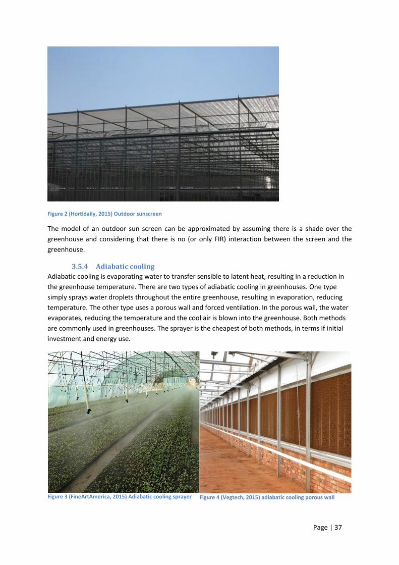
Page | 37

Figure 2 (Hortidaily, 2015) Outdoor sunscreen

The model of an outdoor sun screen can be approximated by assuming there is a shade over the

greenhouse and considering that there is no (or only FIR) interaction between the screen and the

greenhouse.

3.5.4 Adiabatic cooling

Adiabatic cooling is evaporating water to transfer sensible to latent heat, resulting in a reduction in

the greenhouse temperature. There are two types of adiabatic cooling in greenhouses. One type

simply sprays water droplets throughout the entire greenhouse, resulting in evaporation, reducing

temperature. The other type uses a porous wall and forced ventilation. In the porous wall, the water

evaporates, reducing the temperature and the cool air is blown into the greenhouse. Both methods

are commonly used in greenhouses. The sprayer is the cheapest of both methods, in terms if initial

investment and energy use.

Figure 3 (FineArtAmerica, 2015) Adiabatic cooling sprayer

Figure 4 (Vegtech, 2015) adiabatic cooling porous wall

Page | 38

The porous wall is not literally used in this thesis, but the biobed had the same effect. In this thesis

only the adiabatic cooling sprayer is tested as climate actuator. One might think, the air leaving the

biobed is fully saturated, so no more adiabatic cooling can take place. This however is not true, the

air coming from the biobed heats up in the greenhouse while maintaining the same absolute

humidity. The relative humidity therefore lowers to up to and RH of 60% on hot days, as can be seen

in the graph below. These days need cooling the most.

Figure 5 Greenhouse temperature and greenhouse humidity

For testing this method, a few assumptions need to be made.

It is assumed that this method for cooling does not have any shade effects. On hot days that this

system should be active, the light intensity is far beyond the light saturation point of 75𝑊

𝑚2, so minor

shades from the droplets do not influence the growth rate.

The second assumption is that high humidity, and vapour droplets are no problem for duckweed. The

humidity no problem for duckweed because it grows in water and is used to wet situation. The

duckweed will not suffocate from water droplets because leaf surface is hydrophobic, resulting in

water droplets sliding of the crop.

4 Materials and methods The four most important parameters describing the growth of a plant as function of temperature are:

the maximum growth rate and the maximum, minimum and optimal growth temperature (Yan and

Hunt, 1999).Yet, the exact maximum temperature is still unknown. The behaviour of the duckweed

Page | 39

above this temperature is also unknown. Stanley and Madewell (1976) observed that in general,

fronds killed by heat treatment became bleached after three days.

4.1 Test setup The test setup must meet several requirements:

- Growth of duckweed must be measured.

o The growth curve can be non linear.

- Temperature of the duckweed must be measured.

- Growth medium must not be a limiting factor.

- Radiation must not be a limiting factor.

- Temperature of the duckweed must be constant.

- Temperature gradient in the thermostatic bath must be low and at different containers must

be equal.

- Switching between extreme and optimal temperature must be fast.

- Control and measurements must work autonomous and continue during the night.

In the design process, the requirements are taken into account.

4.2 Components In the pictures below an overview of the test setup is given

Figure 6 Thermostatic bath with samples

Page | 40

Figure 7 data logger and par lamp

4.2.1 Thermostatic bath

The thermostatic bath is filled with water from the right temperature. In this thermostatic bath the

sample tubes will be hung. There will not be any direct contact between the thermostatic bath water

and the water inside the sample tubes. The thermostatic bath is 110 centimetres long, 60

centimetres wide and 20 centimetres high. The water level in the thermostatic bath is 15 centimetres

high. Water lost by evaporation is manually refiled every day.

Figure 8 Tube holder from www.labconusa.com

Page | 41

4.2.2 Heater

Figure 9 Fisher Scientific Polystat 37 from www.mmsidz.com

To control the temperature in the thermostatic bath, the Fisher Scientific Polystat 37 is used. This

device has an integrated feedback controller with a temperature stability is +- 0.02°C and the

absolute temperature calibration of +- 3°C. Because of the high absolute temperature difference the

set point of the Polystat 37 may differ from the desired temperature. Therefore the temperature of

the duckweed is measured with thermocouples (chapter 4.2.7) and the set point is adjusted

according to these measurements. The heater has a power of 2.0 kW. The device has a working range

of 20-200°C, the minimum working temperature is dependent on the ambient temperature, because

no external cooler is attached. Temperature selection is performed digitally and can be selected at a

resolution of 0.1°C

The circulation pump has a flow rate of 15l/min and is divided into two channels. Once channel

pumps water directly from the heater to the thermostatic bath. The other channel pumps water via a

tube to the farthest corner from the heater of the container. This way the water in the container is

steered and it is assumed the thermostatic bath has a perfect homogeneous temperature.

4.2.3 Growth container

As growth container, first square containers of a dimension of 18 cm long, 12 cm width and 7

centimetres high were used. During the experiment is was found that it is difficult to keep the

population in these containers clean. After 3 days of testing an algae population started to develop in

these containers.

Page | 42

Figure 10 50ml growth container from www.ecx.images-amazon.com

4.2.4 Par lamp

Duckweed needs PAR light to grow. In the first experiment a 1200 W halogen lamp was used. This

lamp produced enough PAR, but it was found that it produced to much heat and its lifetime was too

short to conduct one experiment. Because of these complication we searched for another lamp, this

was an MASTER Green Power CG T 600W Mogul 1SL with an HS 2000 Armature. This light setup is

commonly used in greenhouses. This lamp has a high emittance of PAR light ad a low emittance of

Infra-red radiation. This is essential, because infra-red radiation is not needed for photosynthesis but

influences the temperature of the duckweed and thus the experiment. The lamp itself produces 80

W of direct heat, this is not influencing the duckweed. The lamp has an average lifetime of 32000

hours which is more than enough to conduct an experiment without a failing lamp. It has an ignition

time of ten seconds to start emitting light and thereafter needs five minutes before it has the right

temperature to emit the right light composition. These five minutes the light composition is not

optimal, but on a photo period of sixteen hours, this can be neglected.

This light is switched on at 6:00 and switched off at 22:00, giving a photo period of 16 hours. This is

not lethal to duckweed (chapter 2.2.1.2). These start and end times are chosen because from the

sunrise to sunset, the duckweed might get enough solar energy to start growing. Because all the

experiments need the same conditions, the light is switched on. When the light is on, the PAR

intensity is around 600 umol/s. this is above the situation point for photosynthesis for duckweed, but

not lethal (2.2.1.1). Above this light intensity a little les or more light does not influence the growth

rate.

Light Technical Characteristics

Colour Code 220 [CCT of 2000K]

Colour Temperature 2000 K

Page | 43

Photosynthetic Photon Flux PPF 1100 umol/s

Energy Used 600 W

Ignition Time 10 (max) s

Run-up time 90% 5 (max) min

Re-ignition Time [min] 1 (max) min

Energy Efficiency Label (EEL) A++

Mercury (Hg) Content 30.0 mg

Energy consumption kWh/1000h 680 kWh

Figure 11 MASTER Green Power CG T 600W Mogul 1SL from www.hortilux.nl

Figure 12 HS200 armature with MASTER Green Power CG T 600W Mogul 1SL from www.hortilux.nl

4.2.5 Growth medium

Duckweed needs more than water and light to survive. In the growth medium essential nutrients are

solved. The concentration of these nutrients must not be a limiting factor.

For the estimation of nutrient concentration, we assume a growth rate that is only possible in theory.

If one can produce a growth medium no limiting for this high growth rate, one is sure it is not limiting

the growth in a real situation. For this reason a growth rate of 100kg dry weight of duckweed per

hectare per day is assumed. The growth rate is recalculated to surface of the duckweed container.

Concentrations of nutrients in Lemna minor are found in Landolt et al. (1987). In this same book, the

limiting concentration of nutrients in a growth medium are found. The experiment lasts seven days.

The volume of growth medium is 20 ml. The surface pf the duckweed is 𝜋 ∗ 1.52 = 7.1𝑐𝑚2.

http://www.hortilux.nl/wp-content/uploads/2013/04/HS2000-2.jpg

Page | 44

Equation 4.2.5-1

𝑇𝑜𝑡𝑎𝑙𝑁𝑢𝑡𝑟𝑖𝑒𝑛𝑡𝐶𝑜𝑛𝑠𝑢𝑚𝑝𝑡𝑖𝑜𝑛

= 𝑃𝑟𝑜𝑑𝑢𝑐𝑡𝑖𝑜𝑛𝐴𝑟𝑒𝑎 ⋅ 𝑃𝑟𝑜𝑑𝑢𝑐𝑡𝑖𝑜𝑛𝑃𝑒𝑟𝐴𝑟𝑒𝑎

⋅ 𝐶𝑜𝑛𝑐𝑒𝑛𝑡𝑟𝑎𝑡𝑖𝑜𝑛𝑂𝑓𝑇ℎ𝑒𝑁𝑢𝑡𝑟𝑖𝑒𝑛𝑡𝐼𝑛𝑠𝑖𝑑𝑒𝑇ℎ𝑒𝐷𝑢𝑐𝑘𝑤𝑒𝑒𝑑 ⋅ 𝐷𝑎𝑦𝑠𝑂𝑓𝐸𝑥𝑝𝑒𝑟𝑖𝑚𝑒𝑛𝑡

Equation 4.2.5-2

𝑅𝑒𝑞𝑢𝑖𝑟𝑒𝑑𝑁𝑢𝑡𝑟𝑖𝑒𝑛𝑡𝑠

= 𝑇𝑜𝑡𝑎𝑙𝑁𝑢𝑡𝑟𝑖𝑒𝑛𝑡𝐶𝑜𝑛𝑠𝑢𝑚𝑝𝑡𝑖𝑜𝑛 + 𝑉𝑜𝑙𝑢𝑚𝑒𝑂𝑓𝐶𝑜𝑛𝑡𝑎𝑖𝑛𝑒𝑟

⋅ 𝑀𝑖𝑛𝑖𝑚𝑢𝑚𝐶𝑜𝑛𝑐𝑒𝑛𝑡𝑟𝑎𝑡𝑖𝑜𝑛

With the method described above the following amount of nutrients is calculated.

Composition stock solution per litre

Required nutrient

Concentration in stock solution[g/l]

Required volume of stock solution[ml]

Consumed by the duckweed after one week [mg]

Minimum concentration after a week[mg/l]

2 gram MnSO4. H2O (169.02 gr/mole) Mn 0.649627

0.437053

0.08874 0.001

2.7 gram H3Bo3 (61.83 gr/mole) B 0.471616

Trace amount

Trace amount

0.5 gram ZnSO4.5H2O (287.54 gr/mole) Zn 0.113723

0.04488 0.005

78 mg CuSO4.5H2O (249.68 gr/mole) Cu 0.019837

0.00867 0.005

126 mg Na2MoO4.2H2O (241.9 gr/mole) Mo 0.049952

Trace amount

Trace amount

Fe Fe 1.116 0.354 0.39525 0.05

KH2PO4

K 35.33652

0.182

6.375 3.28

P 28.01616 5.100 2.55

Ca(NO3)2.4H2O

Ca 2.547649

1.250

3.1875 1.87

N 1.778907 21.93 8.42

MgSO4.7H2O Mg 5.572037 0.320 1.785 0.30 Table 1 nutrient concentration growth medium

4.2.6 Camera

The camera used in this experiment is the ATV Marlin F-145C2 from National Instruments. The

reason to choose this camera is:

It has a good colour depth (12 bits).

Resolution high enough to distinguish single duckweed fronds.

It is fully supported by the LabVIEW software, making calibration easy.

Page | 45

Figure 13 ATV Marlin F-145C2 from www.bilder3.eazyauction.de

Technical Specifications Marlin F-145C2

Max Frame Rate 10 Hz

Spectrum Visible Light

Colour depth 12 bits

Connection IEEE 1394 (fire wire)

Resolution 1392x1040 pixels Table 2 Technical Specifications Marlin F-145C2

4.2.6.1 Lenses

For the lenses, a Pentax C60402 is a C-mount lens is used. This lens designed for 1/2-inch CCD

industrial cameras. The lens has a fast f/1.6 aperture for good low-light images. The lens covers more

than 86°. This is a manual iris lens with fixed focus. The iris can be closed down to f/16 to control

brighter lighting conditions which is needed to take photos when the PAR lamp is on. The wide view

of the lens make it possible for the camera to stand close to the setup and still picture everything. A

major consequence of this is that is creates a large barrel distortion, but here can be calibrated for

(paragraph 4.2.6.3).

Mount C-Mount

Image Format 1/2 CCD

Focal Length 4.2 mm

Aperture f/1.6 to Closed

Iris Type Manual

Focus Type Fixed

Horizontal View Angle 86.77°

4.2.6.2 Calibration

There are two types of calibration spectral and spatial calibration.

Spectral calibration is calibrating the intensity if the pixels. The camera used in this experiment is

already calibrated for the linearity of the sensor, value. The relationships between the different

colour pixels is also dependent on the environment. During the measurements specific light

conditions are present. The measurements happen indoor and an artificial light source present.

These factors influence the light composition. But luckily, here fore can be calibrated. This is done by

letting the camera look at an grey field. When looking at a grey field, a paper with RGB code

(122,122,122), the histograms of the three different colours should all be the same. Because the

Page | 46

sensor shows linear behaviour, the sensor value can be multiplied by a constant to make the

histograms match. This calibration is done with the help of the LabVIEW software. In this software

package one can simple slide three sliders representing these constants. It is assumed that during the

measurements the light conditions were constant.

Spatial calibration is calibrating the camera its pixel size. When taking a picture, not all pixels

represent the same real world size. This deformation is dependent on the lens and lens settings

(Figure 6). This spatial calibration is needed when using a camera to measure area. A calibration grid,

a paper with black dots evenly distributed over the paper, is printed. The camera is mounted in its

experimental condition and the calibration grid is placed on the place where the duckweed would be.

The spatial calibration is also done with the help of the LabVIEW software. When LabVIEW is given

the picture of the calibration grid, and the real world distance between the dots, it will calibrate

camera automatically.

Figure 6 On the left is the camera sensor, on the right the real world area covered by one pixel. From www.allphotolenses.com

4.2.7 Temperature sensor

For the temperature measurements a type K(chromel - alumel) thermocouple is used. This

thermocouple has a sensitivity of approximately 41 µV/°C and a range of -200°C - 1350°C. The sensor

is linear at temperatures to 185°C. For this experiment the temperature of the surface of every

container is measured with this K-type thermocouple. How the measurements of the produced

voltage are done can be found in the next paragraph. PAR sensor

4.2.8 PAR sensor

The PAR- intensity (Photo synthetically Active Radiation) is an important growth factor. In this

experiment, the Apogee Instruments QSO-S PAR Photon Flux Sensor is used to measure the PAR-

intensity. The PAR-sensor only measures wavelengths of (400-700) has a range of 0 to 5,000 μmol

m2s-1 with an output of 0 – 1000 mV.

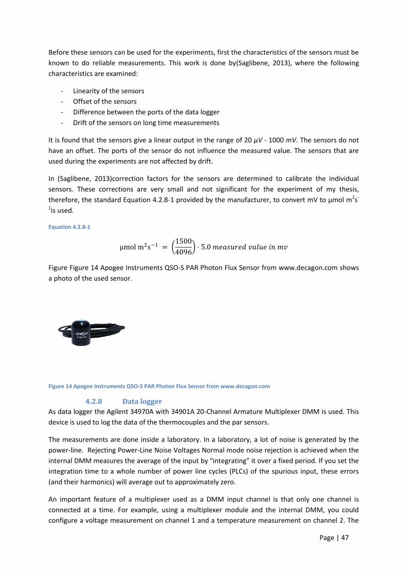
Page | 47

Before these sensors can be used for the experiments, first the characteristics of the sensors must be

known to do reliable measurements. This work is done by(Saglibene, 2013), where the following

characteristics are examined:

- Linearity of the sensors

- Offset of the sensors

- Difference between the ports of the data logger

- Drift of the sensors on long time measurements

It is found that the sensors give a linear output in the range of 20 μV - 1000 mV. The sensors do not

have an offset. The ports of the sensor do not influence the measured value. The sensors that are

used during the experiments are not affected by drift.

In (Saglibene, 2013)correction factors for the sensors are determined to calibrate the individual

sensors. These corrections are very small and not significant for the experiment of my thesis,

therefore, the standard Equation 4.2.8-1 provided by the manufacturer, to convert mV to μmol m2s-

1is used.

Equation 4.2.8-1

μmol m2s−1 = (1500

4096) ⋅ 5.0 𝑚𝑒𝑎𝑠𝑢𝑟𝑒𝑑 𝑣𝑎𝑙𝑢𝑒 𝑖𝑛 𝑚𝑣

Figure Figure 14 Apogee Instruments QSO-S PAR Photon Flux Sensor from www.decagon.com shows

a photo of the used sensor.

Figure 14 Apogee Instruments QSO-S PAR Photon Flux Sensor from www.decagon.com

4.2.8 Data logger

As data logger the Agilent 34970A with 34901A 20-Channel Armature Multiplexer DMM is used. This

device is used to log the data of the thermocouples and the par sensors.

The measurements are done inside a laboratory. In a laboratory, a lot of noise is generated by the

power-line. Rejecting Power-Line Noise Voltages Normal mode noise rejection is achieved when the

internal DMM measures the average of the input by “integrating” it over a fixed period. If you set the

integration time to a whole number of power line cycles (PLCs) of the spurious input, these errors

(and their harmonics) will average out to approximately zero.

An important feature of a multiplexer used as a DMM input channel is that only one channel is

connected at a time. For example, using a multiplexer module and the internal DMM, you could

configure a voltage measurement on channel 1 and a temperature measurement on channel 2. The

Page | 48

instrument first closes the channel 1 relay, makes the voltage measurement, and then opens the

relay before moving on to channel 2 (called break-before-make switching)(Agilent). Therefore one

data logger can be used to measure different channels and sensor types.

4.2.8.1 Temperature measurement

The temperature is measured using thermocouples. A problem with thermocouples is that

connecting them to the data logger creates another thermocouple at the connection. The type of

thermocouple is known, so if one knows the temperature of the connection, a correction can be

calculated. To do this, the DMM has a Built-in thermocouple reference junction, which measures the

temperature of the connections with the data logger. To make sure the reference sensor and the

connections are at the same temperature, an isothermal block is used to make the connections. An

isothermal block is an electrical insulator, but a good heat conductor. An example for thermocouple

type J(in the experiment a k type is used) is given in figure Figure 7.

Figure 7 Built-in thermocouple reference junction (Agilent)

The calculations to convert the measured voltage and the reference temperature to the measured

temperature are ale performed by pre-programmed software in the Agilent 34970A.

For the temperature measurement, a K-type thermocouple is used. With the measurement

technique describes above the absolute measurement error should be +- 1°C with a temperature

coefficient of 0.03°C.

4.2.8.2 PAR measurement

The par sensor channel is read with a direct current auto scale measurement. The measured voltage

is later converted to the measured par light with the help of Microsoft excel. The conversion formula

is Equation 4.2.8-1.

4.2.9 Data collecting

The PAR-sensors and the thermocouples were both connected to a Agilent 34970A() data logger. Via

RS232 connection, this data logger was connected to a 32 bit PC running Microsoft Windows 7.

Controlling and saving of data from the data logger was done by a standalone National Instruments

LabVIEW 2010, version 10.0f2 32 bit, script written by Ing. Kees van Asselt(Wageningen University). I

Page | 49

have modified that script to also log pictures as data. The data files were logged to a text file and

later imported in Microsoft Office Excel 2010 for further processing. The user logged in on the

computer would automatically be logged of by Wageningen UR software, after several hours of

inactivity. To prevent this from happening, the program Move Mouse version 3.2.0 from

https://movemouse.codeplex.com/ was used. This program moves the mouse every 30 seconds so

the computer will sense activity. This way the data collection can continue day and night.

4.3 Methods First, the duckweed will be grown at optimal conditions, the duckweed can accumulate to the growth

medium. When the accumulation is done, the duckweed sample containers will be placed in the hot

water container. Because of the small volume of the duckweed samples and the relatively large area

of the containers, the time constant is low and the temperature reaches the steady state quickly.

After the exposure to the high temperature, the duckweed containers will be placed back to optimal

conditions. At optimal growth conditions, the duckweed will be monitored for one week. For the

temperature response of the system and the temperature maintenance see chapter 5.1.

To get an idea of the lethal times of exposure at a given temperature, an estimation is made. This

estimation is done by extrapolating formula 2.1.3-1. Herby it is assumed that LD50 (50 % of the

population dies) is good enough for analysis. To move the samples from high to low temperature, a

human is needed. I could only enter the laboratory between 7:00 and 22:00 on Monday to Friday and

between 9:00 and 17:00 during the weekend. Besides that, I also had my own agenda. The result of

these complications were the following exposure times.

Temperature (°C) 35.6 37.3 39.1 40.9

Expected time of LD 50 (hours) 86 32 11 4

Sample time 1 (hours) 0 0 0 0

Sample time 2 (hours) 23.75 4 2 2

Sample time 3 (hours) 44.5 7.5 4 3

Sample time 4 (hours) 48 20.5 6 4

Sample time 5 (hours) 62 24 8 5

Sample time 6 (hours) 65 27.5 10 6

Sample time 7 (hours) 70 31 12 7 Table 3 Times of exposure to high temperature

Based on the existing model, the control population and these measurements, the death rate can be

determined. It is close to impossible to determine the death rate directly, because when the

duckweed dies, the death fronds will remain shortly in the healthy population and on the outside

look healthy as well. The photosynthetic activity can be measured using very expensive special

cameras. During my research I didn’t have access to this kind of cameras. Another method to

determine the activity of duckweed is measuring the respiration rate. During my research, I also

didn’t have access to this device. The dry mass of duckweed can be weight. This method does not

distinguish dead fronds from living fronds, it just measures biomass. Dead duckweeds fronds will turn

bleached after three days.

To distinguish living from dead fronds, a camera with digital image processing software is used. The

camera takes a picture twice a day and the vision software calculates the area of living duckweed.

The area of duckweed is, in this method, a measurement for the amount of duckweed. It is assumed

https://movemouse.codeplex.com/

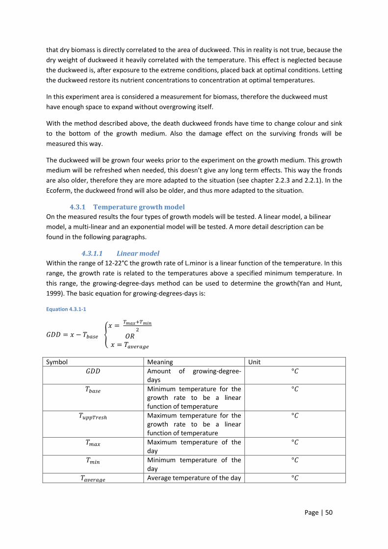
Page | 50

that dry biomass is directly correlated to the area of duckweed. This in reality is not true, because the

dry weight of duckweed it heavily correlated with the temperature. This effect is neglected because

the duckweed is, after exposure to the extreme conditions, placed back at optimal conditions. Letting

the duckweed restore its nutrient concentrations to concentration at optimal temperatures.

In this experiment area is considered a measurement for biomass, therefore the duckweed must

have enough space to expand without overgrowing itself.

With the method described above, the death duckweed fronds have time to change colour and sink

to the bottom of the growth medium. Also the damage effect on the surviving fronds will be

measured this way.

The duckweed will be grown four weeks prior to the experiment on the growth medium. This growth

medium will be refreshed when needed, this doesn’t give any long term effects. This way the fronds

are also older, therefore they are more adapted to the situation (see chapter 2.2.3 and 2.2.1). In the

Ecoferm, the duckweed frond will also be older, and thus more adapted to the situation.

4.3.1 Temperature growth model

On the measured results the four types of growth models will be tested. A linear model, a bilinear

model, a multi-linear and an exponential model will be tested. A more detail description can be

found in the following paragraphs.

4.3.1.1 Linear model

Within the range of 12-22°C the growth rate of L.minor is a linear function of the temperature. In this

range, the growth rate is related to the temperatures above a specified minimum temperature. In

this range, the growing-degree-days method can be used to determine the growth(Yan and Hunt,

1999). The basic equation for growing-degrees-days is:

Equation 4.3.1-1

𝐺𝐷𝐷 = 𝑥 − 𝑇𝑏𝑎𝑠𝑒 {

𝑥 = 𝑇𝑚𝑎𝑥+𝑇𝑚𝑖𝑛

2

𝑂𝑅𝑥 = 𝑇𝑎𝑣𝑒𝑟𝑎𝑔𝑒

Symbol Meaning Unit

𝐺𝐷𝐷 Amount of growing-degree-days

°𝐶

𝑇𝑏𝑎𝑠𝑒 Minimum temperature for the growth rate to be a linear function of temperature

°𝐶

𝑇𝑢𝑝𝑝𝑇𝑟𝑒𝑠ℎ Maximum temperature for the growth rate to be a linear function of temperature

°𝐶

𝑇𝑚𝑎𝑥 Maximum temperature of the day

°𝐶

𝑇𝑚𝑖𝑛 Minimum temperature of the day

°𝐶

𝑇𝑎𝑣𝑒𝑟𝑎𝑔𝑒 Average temperature of the day °𝐶

Page | 51

Where 𝑇𝑚𝑎𝑥 and 𝑇𝑚𝑖𝑛 are daily maximum and minimum air temperature. 𝑇𝑚𝑎𝑥+𝑇𝑚𝑖𝑛

2 is an

approximation of the average temperature of that day. 𝑇𝑏𝑎𝑠𝑒 is the base temperature, the lowest

temperature for the growth process to take place. The crop production is the integral of the

linearized growth function as function of T(GDD).

Equation 4.3.1-2

𝑃 = 𝑓(𝑇 → 𝐺𝐷𝐷)

4.3.1.2 Bilinear model

The linear model is only accurate in the linear part of the growth function. The linear model fails to

account for the fact that temperatures above the optimal temperature (𝑇𝑜𝑝𝑡) inhibit the growth rate.

The bilinear model does account for growth inhibition for temperatures above 𝑇𝑜𝑝𝑡. This is done with

use of a second linear equation for temperatures above 𝑇𝑜𝑝𝑡.

Equation 4.3.1-3

{𝑟 = 𝑎1 + 𝑏1𝑇 𝑖𝑓(𝑇 < 𝑇𝑜𝑝𝑡)

𝑟 = 𝑎2 + 𝑏2𝑇 𝑖𝑓(𝑇 > 𝑇𝑜𝑝𝑡)

This bilinear approach still is not accurate for all temperatures. Around the optimal temperature, the

growth rate is not a linear function of temperature as can be seen in figure 1 and 2. Also the growth

rate around the minimum and maximum temperature is not accurate.

4.3.1.3 Multi-linear model

A multi-linear model is a composed of three or more linear functions. With the use of more linear

functions, the growth rate can be accurately approximated at all the temperatures, as long as one

can (experimentally) determine the parameters required for each linear function. A huge

disadvantage of the multi-linear model is the amount of required data to compose the model.

Another problem is the calibration, the large amount of required parameters renders the approach

subject to calibration errors(Yan and Hunt, 1999).

4.3.1.4 Exponential and polynomial model

There are reasons to believe that temperature response of a given process should be a smooth

curve((Yan and Hunt, 1999), rather than a rigid combination of linear equations, which introduce

abrupt changes. Exponential and polynomials give smooth functions which with the right parameters

should be able to predict the growth rate more accurately. A disadvantage of the exponential growth

function is that is does not simulate the response to high temperatures, because it does not allow for

a reduced growth rate for temperatures above the optimum.

5 Experimental results

5.1 Temperature in the test setup The temperature response of the reaction tubes is fast enough for the experiment. In the graph

below a temperature response of a growth container from 36°C to the optimal temperature of

approximately 26 degrees is shown. One can see that within 10 minutes the desired temperature of

approximately 26°C is reached.

Page | 52

Figure 8 temperature response of a growth container

As said before, the thermostatic bath should maintain a stable temperature, and this should also be

the case for the growth containers. In the graph below one can see that the temperature in the

thermostatic bath differs only +- 0.2 °C and the temperature of the reaction tubes only are up to

0.8°C lower and differ maximum 0.2°C from their average.

Figure 9 temperature maintenance

25

27

29

31

33

35

370

:00

0:0

2

0:0

5

0:0

8

0:1

1

0:1

4

0:1

7

0:2

0

0:2

3

0:2

6

0:2

9

0:3

2

0:3

5

0:3

8

0:4

1

0:4

4

0:4

7

0:5

0

0:5

3

tem

pe

ratu

re °

C

time in hours and minutes

Temperature response growth container

growth container

35

35.2

35.4

35.6

35.8

36

36.2

0:0

0

0:1

0

0:2

1

0:3

2

0:4

3

0:5

4

1:0

5

1:1

6

1:2

7

1:3

8

1:4

9

2:0

0

2:1

1

2:2

2

2:3

3

2:4

4

2:5

5

3:0

6

3:1

7

tem

pe

ratu

re °

C

time in hours and minutes

Temperature maintenance

container bottom coverd

container surface not coverd

container bottom not coverd

thermobath centre

Page | 53

5.1 Temperature growth curve In the conducted experiment the growth rate of duckweed as function of temperature and time of

exposal was tested. The amount of measured duckweed, in the form of area of healthy duckweed in

pixels, can be found in appendix 10.2. Analysis as described in chapter 4.3 is described has failed.

Interpreting the data was more difficult than expected and I was running out of time.

To analyse the production of duckweed at the Ecoferm when the duckweed is able to die, and to test

the climate actuators mentioned in chapter 3.5 a model describing the behaviour of duckweed at

these temperatures is needed. To continue my research, a few assumptions are made based on

intuitive interpretation of the data in appendix 10.2.

It can noticed that with an exposure temperature of 40.9°C the duckweed dies, even with an

exposure time of two hours. This will be approximated in the model by assuming that with a

temperature of 40.9°C the duckweed instantly dies and the duckweed population needs to be

restored from an external input. This will be simulated by setting the mat density to 10% of the

desired situation.

At the temperatures of 35.6°C and higher, one can see that the amount of duckweed decreases, but

restores after a while. This will be approximated by setting the growth rate of the duckweed to zero

when a temperature of 35.6°C or higher is present.

5.2 Duckweed climate In this chapter the results of the simulation of the climate actuators is presented. The associated

graphs can be found in appendix 10.3.

5.2.1 Duckweed without climate control

Has a total dry weight production of 1991.8 kg/year. During the period from day 140 till 220 the

duckweed is only harvested once, because during this period the temperature of 40.6°C is reached

several times.

5.2.2 Extra ventilation

The maximum ventilation is increased to 150 m3/s instead of 98.3m3/s. Also a simple controller is

applied, when the temperature rises above 26°C the ventilator will blow full power. This resulted in a

production of 2774.6 kg dry matter per year.


The adiabatic cooler was set to start cooling when the duckweed temperature rises above 26°C. The

adiabatic cooler has a max capacity to evaporate 0.01 gram vapour for every kg of dry air present.

With these setting a total yield of 2713.2 kg dry matter per year could be achieved. When looking at

Figuur 26 Duckweed temperature in the appendix, one can see that the temperature does not rise

above 40°C, this means the duckweed doesn’t die. This is also confirmed by the mat density (Figure.

Page | 54

5.2.4 Whitewash

The tested whitewash has a reflectance of 50%. Her fore, only 50% of the solar energy can be used

for heating the greenhouse. A consequence is that the duckweed also gets less sunlight. With the

whitewash a total production of 2171.4 kg dry matter will be produced in one year.

5.2.5 Thermal screen

The mathematical model of the thermal screen is difficult and I was running out of time, so this is not

tested.

6 Discussion

6.1 Experiment In general the test setup worked, the time constant of the duckweed temperature was fast enough

for assuming an instant temperature transition. The temperature control was stable. The growth

medium was not exhausted during the experiment and the light intensity was sufficient. Still the

results were not useful for construction for a dynamic model of the duckweed death rate at high

temperatures.

Measuring when a duckweed frond is dead is difficult, because with simple sensors it is impossible to

directly measure if a frond has died. There are sensors able to directly measure the photosynthetic

activity of a plant. These sensors are very expensive and were not available.

The camera was able to distinguish dead and living crops after the frond had four days time to turn

white. If the area of duckweed is representative for amount of biomass in the duckweed population

is not tested.

Modelling the death rate of duckweed, using the growth of the area of living duckweed and

comparing it to a control group, didn’t work in the setup mentioned in chapter 4.1. One of the

reasons was the available area in the growth containers. During the experiment, the duckweed in the

control containers was growing too much that it needed more space than available in the container.

Because of this duckweed frond started growing over each other, making it impossible to measure

using a RGB camera. Therefore the growth rate of the control group as not correct.

When the initial amount of duckweed will be lowered, the possibility of a too small population

becomes present. Therefore larger growing containers are recommended, with a small initial amount

of duckweed.

6.2 Model

6.2.1 Whitewash

The assumption made for the climate actuators are rough assumptions. The whitewash does

decrease the transmittance of the roof, and increase its reflection, but also increases its radiation

absorption and insulation. Increasing the indoor temperature of the greenhouse.

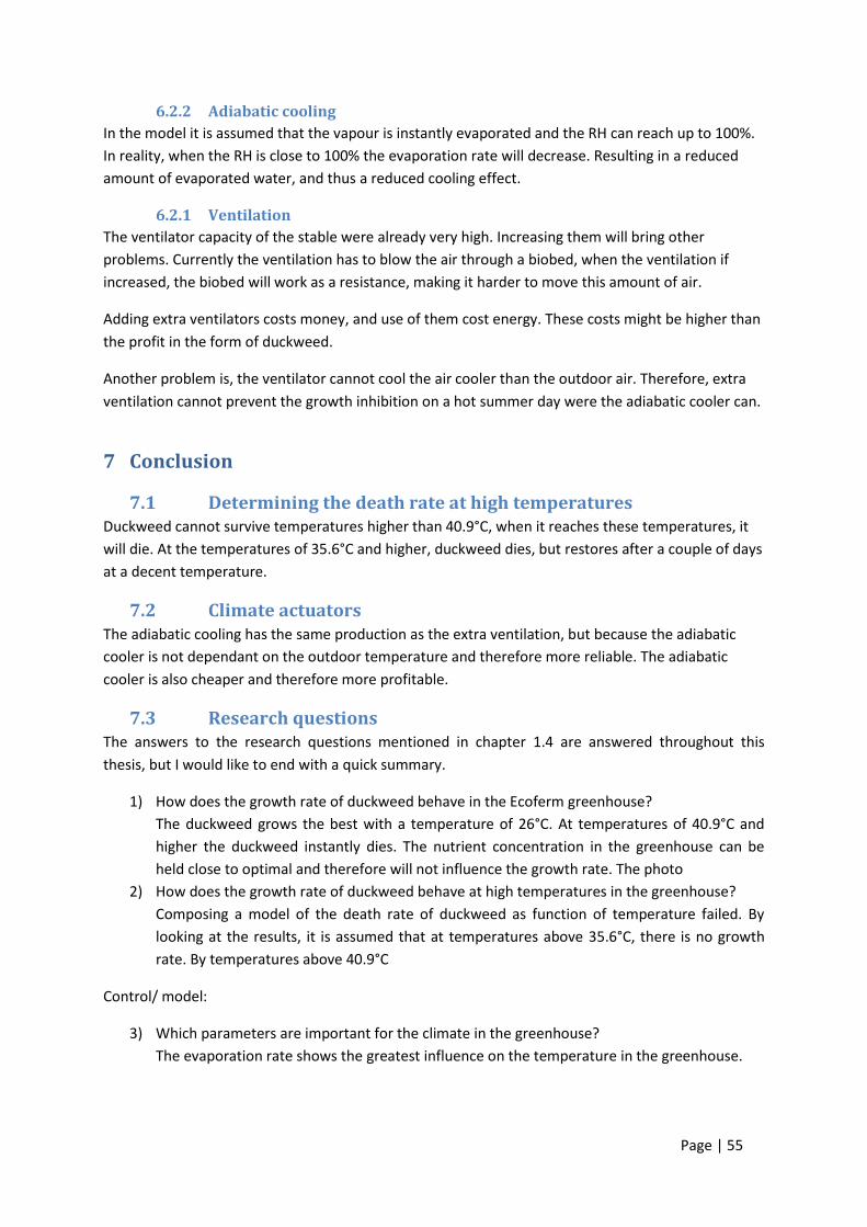
Page | 55


In the model it is assumed that the vapour is instantly evaporated and the RH can reach up to 100%.

In reality, when the RH is close to 100% the evaporation rate will decrease. Resulting in a reduced

amount of evaporated water, and thus a reduced cooling effect.

6.2.1 Ventilation

The ventilator capacity of the stable were already very high. Increasing them will bring other

problems. Currently the ventilation has to blow the air through a biobed, when the ventilation if

increased, the biobed will work as a resistance, making it harder to move this amount of air.

Adding extra ventilators costs money, and use of them cost energy. These costs might be higher than

the profit in the form of duckweed.

Another problem is, the ventilator cannot cool the air cooler than the outdoor air. Therefore, extra

ventilation cannot prevent the growth inhibition on a hot summer day were the adiabatic cooler can.

7 Conclusion

7.1 Determining the death rate at high temperatures Duckweed cannot survive temperatures higher than 40.9°C, when it reaches these temperatures, it

will die. At the temperatures of 35.6°C and higher, duckweed dies, but restores after a couple of days

at a decent temperature.

7.2 Climate actuators The adiabatic cooling has the same production as the extra ventilation, but because the adiabatic

cooler is not dependant on the outdoor temperature and therefore more reliable. The adiabatic

cooler is also cheaper and therefore more profitable.

7.3 Research questions The answers to the research questions mentioned in chapter 1.4 are answered throughout this

thesis, but I would like to end with a quick summary.

1) How does the growth rate of duckweed behave in the Ecoferm greenhouse?

The duckweed grows the best with a temperature of 26°C. At temperatures of 40.9°C and

higher the duckweed instantly dies. The nutrient concentration in the greenhouse can be

held close to optimal and therefore will not influence the growth rate. The photo

2) How does the growth rate of duckweed behave at high temperatures in the greenhouse?

Composing a model of the death rate of duckweed as function of temperature failed. By

looking at the results, it is assumed that at temperatures above 35.6°C, there is no growth

rate. By temperatures above 40.9°C

Control/ model:

3) Which parameters are important for the climate in the greenhouse?

The evaporation rate shows the greatest influence on the temperature in the greenhouse.

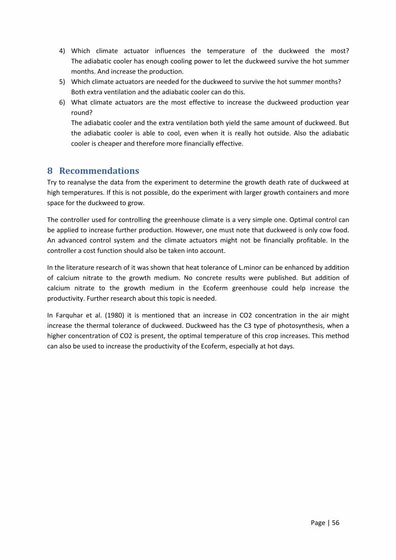
Page | 56

4) Which climate actuator influences the temperature of the duckweed the most?

The adiabatic cooler has enough cooling power to let the duckweed survive the hot summer

months. And increase the production.

5) Which climate actuators are needed for the duckweed to survive the hot summer months?

Both extra ventilation and the adiabatic cooler can do this.

6) What climate actuators are the most effective to increase the duckweed production year

round?

The adiabatic cooler and the extra ventilation both yield the same amount of duckweed. But

the adiabatic cooler is able to cool, even when it is really hot outside. Also the adiabatic

cooler is cheaper and therefore more financially effective.

8 Recommendations Try to reanalyse the data from the experiment to determine the growth death rate of duckweed at

high temperatures. If this is not possible, do the experiment with larger growth containers and more

space for the duckweed to grow.

The controller used for controlling the greenhouse climate is a very simple one. Optimal control can

be applied to increase further production. However, one must note that duckweed is only cow food.

An advanced control system and the climate actuators might not be financially profitable. In the

controller a cost function should also be taken into account.

In the literature research of it was shown that heat tolerance of L.minor can be enhanced by addition

of calcium nitrate to the growth medium. No concrete results were published. But addition of

calcium nitrate to the growth medium in the Ecoferm greenhouse could help increase the

productivity. Further research about this topic is needed.

In Farquhar et al. (1980) it is mentioned that an increase in CO2 concentration in the air might

increase the thermal tolerance of duckweed. Duckweed has the C3 type of photosynthesis, when a

higher concentration of CO2 is present, the optimal temperature of this crop increases. This method

can also be used to increase the productivity of the Ecoferm, especially at hot days.

Page | 57

9 References Agilent. Agilent 34970A manual.34.

Agricolas, N. 2015. Screens for greenhouses. Available at: http://www.novedades-agricolas.com/images/invernaderos/pantallas/portadapant.jpg

Alaerts, G. J., R. Mahbubar, and P. Kelderman. 2000. Performance analysis of a full-scale duckweed-covered sewage lagoon. Water Research 30(4):843-852.

Ashby, E. 1929. The interaction of factors in the growth of lemna. III. The interrelationship of duration and intensity of light. Ann.Bot. 43:333-354.

Ashby, E., and T. A. Oxley. 1935. The interaction of factors in the growth of Lemna. VI. An analysis of the influence of light intensity and temperature on the assimilation rate and the rate of frond multiplication. Ann.Bot. 49:309-336.

Breene, W. M., S. Lin, L. Hardman, and J. Orf. 1988. Protein and oil content of soybeans from different geographic locations. 65(12):1927-1931.

Currey, C. J. 2013. Keeping Cool With Greenhouse Shading. www.greenhousegrower.com. Available at: http://www.greenhousegrower.com/structures-equipment/equipment/keeping-cool-with-greenhouse-shading/.

Evert, R. F., and S. E. Eichhorn. 2013. Biology of Plants. eigth. Peter Marshall.

Farquhar, G. D., S. von Caemmerer, and J. A. Berry. 1980. A biochemical model of photosynthetic CO2 assimilation in leaves of C3 species. 149(1):78-90.

Filbin, G. J., and R. A. Hough. 1985. Photosynthesis, photorespiration, and productivity in Lemna minor L.1. Limnology and Oceanography 30(2):322-334.

FineArtAmerica. 2015. Greenhouse watering. Available at: http://fineartamerica.com/featured/greenhouse-watering-dejan-maksimovic.html.

Haaring, H. 2014. Eurotier 2014 Hanover.

Hodgson, G. L. 1970. Effects of temperature on the growth and development of Lemna minor, under conditions of natural daylight. Ann.Bot. 34:365-381.

Hortidaily. 2015. Outdoor sunscreen. Available at: http://www.hortidaily.com/article/17247/Outer-screen-ideal-solution-for-perfect-climate.

Keller, B., and A. M. S. Costa. 2011. A Matlab GUI for calculating the solar radiation and shading of surfaces on the earth. Computer Applications in Engineering Education 19(1):161-170.

Kempkes, F. 2012. NIR-screen as an energy saving measure.

KNMI. 2009. 2014a. Uurgegevens 260 2001-2010. KNMI, ed. De Bilt.

Kroes, K. 2014. My personel visit to the Ecoferm.

Landolt, E. 1957. Physologische und ökologische Untersuchungen an Lemnaceen. . Ber.Schweiz.Bot.Ges 67(271-410).

http://www.novedades-agricolas.com/images/invernaderos/pantallas/portadapant.jpg

http://www.novedades-agricolas.com/images/invernaderos/pantallas/portadapant.jpg

http://www.greenhousegrower.com/

http://www.greenhousegrower.com/structures-equipment/equipment/keeping-cool-with-greenhouse-shading/

http://www.greenhousegrower.com/structures-equipment/equipment/keeping-cool-with-greenhouse-shading/

http://fineartamerica.com/featured/greenhouse-watering-dejan-maksimovic.html

http://www.hortidaily.com/article/17247/Outer-screen-ideal-solution-for-perfect-climate

http://www.hortidaily.com/article/17247/Outer-screen-ideal-solution-for-perfect-climate

Page | 58

Landolt, E., A. Lueoend, and R. Kandeler. 1987. Biosystematic investigations in the family of duckweeds (Lemnaceae) = Biosystematische Untersuchungen in der Familie der Wasserlinsen (Lemnaceae). Veroeffentlichungen des Geobotanischen Institutes der Eidgenoessische Technische Hochschule, Stiftung Ruebel;Heft 70,71,80,95. E.T.H., Zuerich.

Lasfar, S., F. Monette, L. Millette, and A. Azzouz. 2007. Intrinsic growth rate: A new approach to evaluate the effects of temperature, photoperiod and phosphorus–nitrogen concentrations on duckweed growth under controlled eutrophication. Water Research 41(11):2333-2340.

Lehman, P. W., W. K. Silk, and A. W. Knight. 1981. Protein and Nitrate Content of Lemna Sp. as a Function of Developmental Stage and Incubation Temperature. Plant Physiol 68:127-132.

Liere, J. v., G. Boosten, L. v. Dijk, G. Hemke, and A. Verschoor. 2011. ECOFERM! De kringloopboerderij. InnovationNetwerk. Utrecht.

Lowry, O. H., N. J. Rosebrough, A. L. Farr, and R. J. Randall. 1951. Protein measurement with the folin phenol reagent. Journal of Biological Chemistry 193(1):265-275.

Mashonjowa, E., F. Ronsse, T. Mhizha, J. R. Milford, R. Lemeur, and J. G. Pieters. 2010. The effects of whitening and dust accumulation on the microclimate and canopy behaviour of rose plants (Rosa hybrida) in a greenhouse in Zimbabwe. Solar Energy 84(1):10-23.

McLay, C. L. 1976. The effect of pH on the population growth of three species of duckweed: Spirodela oligorrhiza, Lemna minor and Wolffia arrhiza. Freshwater Biology 6(2):125-136.

Ooster, i. A. v. t. 2014. Buidling Physics and Climate Engineering.

Peeters, E. T. H. M., J. P. van Zuidam, B. G. van Zuidam, E. H. Van Nes, S. Kosten, P. G. M. Heuts, R. M. M. Roijackers, J. J. C. Netten, and M. Scheffer. 2013. Changing weather conditions and floating plants in temperate drainage ditches. Journal of Applied Ecology 50(3):585-593.

Room, P. M. 1986. Equations relating growth and uptake of nitrogen by Salvinia molesta to temperature and the availability of nitrogen. Aquatic Botany 24(1):43-59.

Saglibene, M. 2013. The canyon effect: Decay of diffuse light between vertical plates. Wageningen UR, Biomass Refinery and Process Dynamics, Wageningen The Netherlands

Stanley, R. A., and C. E. Madewell. 1976. Thermal tolerance of Lemna minor L. Circular Z / National fertilizer development center. Tennessee valley authority;no. 73. T.V.A., Muscle Shoals.

Szabó, S., R. Roijackers, M. Scheffer, and G. Borics. 2005. The strength of limiting factors for duckweed during algal competition. Archiv für Hydrobiologie 164(1):127-140.

van den Top, N. 2014. Dynamic modelling of duckweed production on the first ECOFERM! closed-cycle farm for rosé calves. s.n], [S.l.

van der Heide, T., R. M. M. Roijackers, E. H. van Nes, and E. T. H. M. Peeters. 2006. A simple equation for describing the temperature dependent growth of free-floating macrophytes. Aquatic Botany 84(2):171-175.

Vanthoor, B. H. E., C. Stanghellini, E. J. van Henten, and P. H. B. de Visser. 2011. A methodology for model-based greenhouse design: Part 1, a greenhouse climate model for a broad range of designs and climates. Biosystems Engineering 110(4):363-377.

Page | 59

Vegtech. 2015. Cooling. Available at: http://www.vegtech.co.za/products/climate_control/cooling/.

Wedge, R. M., and J. E. Burris. 1982. Effects of light and temperature on duckweed photosynthesis. Aquatic Botany 13(0):133-140.

Yan, W., and L. A. Hunt. 1999. An Equation for Modelling the Temperature Response of Plants using only the Cardinal Temperatures. Annals of Botany.

http://www.vegtech.co.za/products/climate_control/cooling/

Page | 60

10 Appendices

10.1 Camera calibration

Figure 15 calibration grid

Page | 61

Figure 16 Area measurement

10.2 Death rate temperature

10.2.1 Temperature of 40.9°C

0

10000

20000

30000

40000

50000

60000

70000

0 1 2 3 4 5 6

0 hours

sample 1 sample 2

Page | 62

0

5000

10000

15000

20000

25000

0 1 2 3 4 5 6

7 hours

sample 1 sample 2

0

5000

10000

15000

20000

25000

30000

35000

40000

0 1 2 3 4 5 6

6 hours

sample 1 sample 2

0

10000

20000

30000

40000

50000

60000

70000

0 1 2 3 4 5 6

5 hours

sample 1 sample 2

Page | 63

0

10000

20000

30000

40000

50000

60000

0 1 2 3 4 5 6

4 hours

sample 1 sample 2

0

5000

10000

15000

20000

25000

30000

35000

40000

45000

50000

0 1 2 3 4 5 6

3 hours

sample 1 sample 2

0

10000

20000

30000

40000

50000

60000

70000

80000

0 1 2 3 4 5 6

2 hours

sample 1 sample 2

Page | 64

10.2.2 Temperature 39.1°C

0

10000

20000

30000

40000

50000

60000

70000

80000

90000

0 1 2 3 4 5 6 7 8

0 hours

sample 1 sample2

0

10000

20000

30000

40000

50000

60000

70000

0 1 2 3 4 5 6 7 8

12 hours

sample 1 sample2

Page | 65

0

10000

20000

30000

40000

50000

60000

70000

0 1 2 3 4 5 6 7 8

10 hours

sample 1 sample2

0

10000

20000

30000

40000

50000

60000

0 1 2 3 4 5 6 7 8

8 hours

sample 1 sample2

0

10000

20000

30000

40000

50000

60000

70000

80000

0 1 2 3 4 5 6 7 8

6 hours

sample 1 sample2

Page | 66


0

10000

20000

30000

40000

50000

60000

70000

80000

0 1 2 3 4 5 6 7 8

4 hours

sample 1 sample2

0

10000

20000

30000

40000

50000

60000

70000

80000

0 1 2 3 4 5 6 7 8

2 hours

sample 1 sample2

0

10000

20000

30000

40000

50000

60000

70000

80000

90000

100000

0 1 2 3 4 5 6 7

0 hours

sample1 sample2

Page | 67

66000

68000

70000

72000

74000

76000

78000

80000

82000

84000

86000

0 1 2 3 4 5 6 7

31 hours

sample1 sample2

0

10000

20000

30000

40000

50000

60000

70000

80000

90000

0 1 2 3 4 5 6 7

27.5 hours

sample1 sample2

0

10000

20000

30000

40000

50000

60000

70000

80000

90000

0 1 2 3 4 5 6 7

24 hours

sample1 sample2

Page | 68

0

10000

20000

30000

40000

50000

60000

70000

80000

90000

100000

0 1 2 3 4 5 6 7

20.5 hours

sample1 sample2

0

10000

20000

30000

40000

50000

60000

70000

80000

90000

0 1 2 3 4 5 6 7

7.5 hours

sample1 sample2

0

10000

20000

30000

40000

50000

60000

70000

80000

90000

0 1 2 3 4 5 6 7

4 hours

sample1 sample2

Page | 69


0

10000

20000

30000

40000

50000

60000

70000

80000

90000

0 1 2 3 4 5 6

0 hours

sample1 sample2

0

10000

20000

30000

40000

50000

60000

70000

80000

90000

100000

0 1 2 3 4 5 6

70 hours

sample1 sample2

0

10000

20000

30000

40000

50000

60000

70000

80000

90000

100000

0 1 2 3 4 5 6

65 hours

sample1 sample2

Page | 70

0

10000

20000

30000

40000

50000

60000

70000

80000

90000

100000

0 1 2 3 4 5 6

62 hours

sample1 sample2

0

10000

20000

30000

40000

50000

60000

70000

80000

90000

100000

0 1 2 3 4 5 6

48 hours

sample1 sample2

0

10000

20000

30000

40000

50000

60000

70000

80000

90000

100000

0 1 2 3 4 5 6

44.5 hours

sample1 sample2

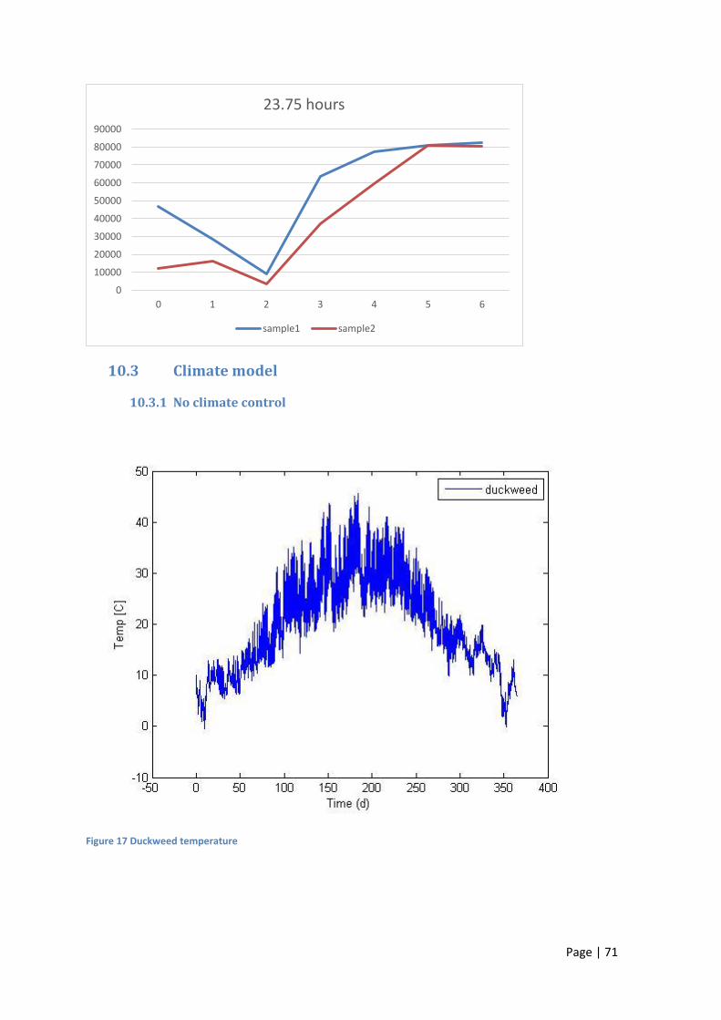
Page | 71

10.3 Climate model

10.3.1 No climate control

Figure 17 Duckweed temperature

0

10000

20000

30000

40000

50000

60000

70000

80000

90000

0 1 2 3 4 5 6

23.75 hours

sample1 sample2

Page | 72

Figure 18 Solar radiation

Page | 73

Figure 19 Mat density

Figure 20 relative humidity

Page | 74

Figure 21 all temperatures

10.3.1 Whitewash

Figure 22 DUckweed temperature

Page | 75

Figure 23 relative humidity greenhouse

Figure 24 mat density

10.3.1 Adiabatic cooler

Page | 76

Figuur 25 Al temperaturs

Figuur 26 Duckweed temperature

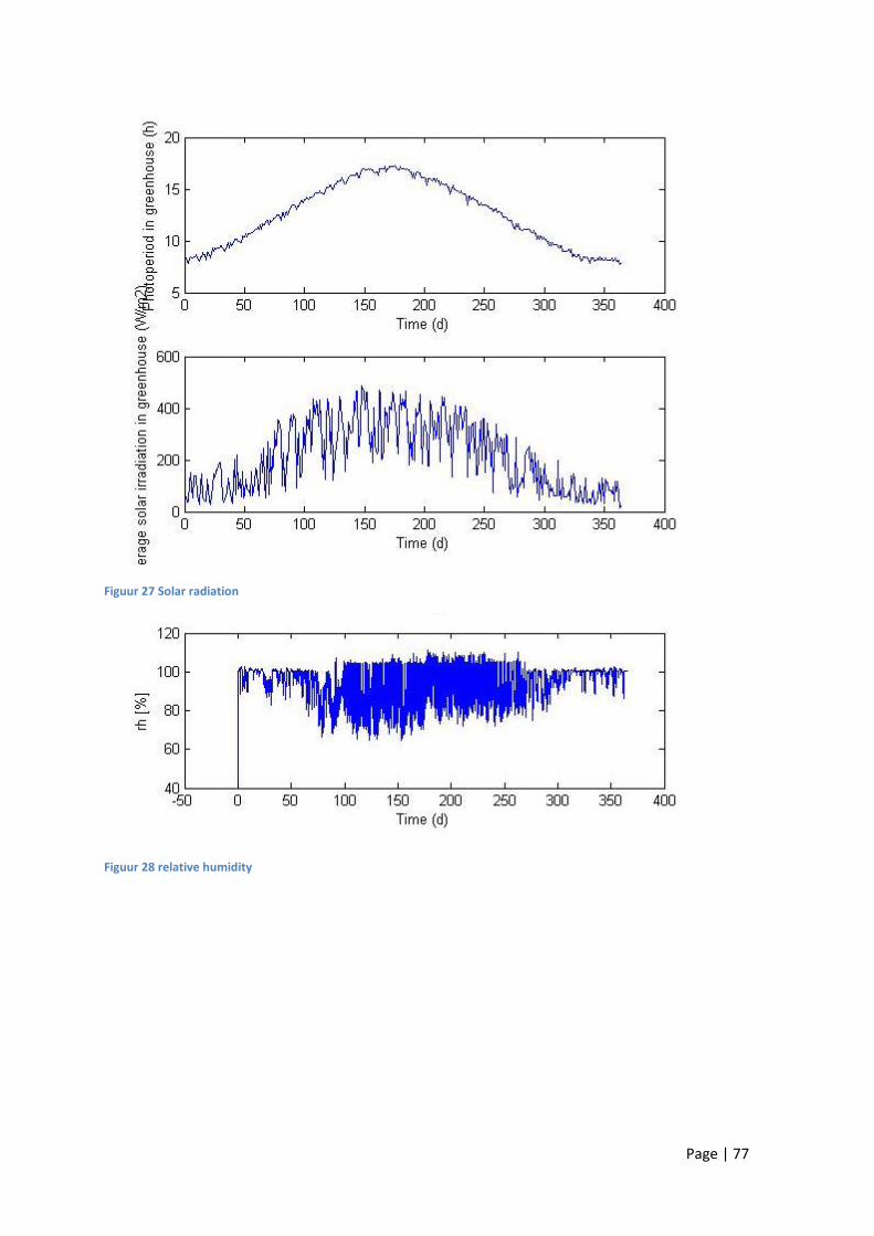
Page | 77

Figuur 27 Solar radiation

Figuur 28 relative humidity

Page | 78

Figuur 29 intrinsic growth rate

Page | 79

Figuur 30 Mat density

10.3.1 Ventilation

Page | 80

Figuur 31 Duckweed temperatrure

Figuur 32 Solar radiation

Page | 81

Figuur 33 mat density

Figuur 34 intrinsic growth rate

Page | 82

Figuur 35 relative humidity

Figuur 36 all temperatures

Temperature response of duckweed growth at the Ecoferm ...

Documents

Transcript of Temperature response of duckweed growth at the Ecoferm ...