1

Temperature Enhanced Effects of Ozone on

Cardiovascular Mortality in 95 Large US Communities,

1987-2000

-- Assessment Using the NMMAPS data

Cizao Ren*

School of Public Health, Queensland University of Technology, Kelvin Grove, QLD4059,

Australia

Tel: +61-7-3138 8298, Fax: +61-7-3138 3369, Email: rencizao@yahoo.com

Gail M Williams

School of Population Health, University of Queensland, Herston, QLD4006, Australia

Telephone: +61-7-33655406, Fax: +61-7-33655599, Email: g.williams@sph.uq.edu.au

Kerrie Mengersen

School of Mathematical Sciences, Queensland University of Technology, Brisbane, QLD4001,

Australia

Telephone: 61-7-31382063, Fax +61-7-3138 2310, e-mail: k.mengersen@qut.edu.au

Lidia Morawska

International Laboratory for Air Pollution Quality and Health, Queensland University of

Technology, Brisbane, QLD4001, Australia

Telephone: 61-7-31382616, Fax +61-7-3138 9079, e-mail: l.morawska@qut.edu.au

Shilu Tong

2

School of Public Health, Queensland University of Technology, Kelvin Grove, QLD4059,

Australia

Tel: +61-7-3138 9745, Fax: +61-7-3138 3369, Email: s.tong@qut.edu.au

Words: 3193 words for text; 246 words for abstract; 40 references; 2 tables and 1 figure

Keywords: Air pollution, Interaction, Mortality, Ozone, Temperature

* Corresponding author (current address):

Dr. Cizao Ren

Harvard School of Public Health

Exposure, Epidemiology and Risk Program

Landmark Center West, 4th Floor

401 Park Drive, Box 15677

Boston MA 02215

Fax: 1-617-384 8728

Phone: (??)

Email: rencizao@yahoo.com

3

Abstract

A few studies examined interactive effects between air pollution and temperature on health

outcomes. This study is to examine if temperature modified effects of ozone and

cardiovascular mortality in 95 large US cities. A nonparametric and a parametric regression

models were separately used to explore interactive effects of temperature and ozone on

cardiovascular mortality during May and October, 1987-2000. A Bayesian meta-analysis was

used to pool estimates. Both models illustrate that temperature enhanced the ozone effects on

mortality in the northern region, but obviously in the southern region. A 10-ppb increment in

ozone was associated with 0.41 % (95% posterior interval (PI): -0.19 %, 0.93 %), 0.27 %

(95% PI: -0.44 %, 0.87 %) and 1.68 % (95% PI: 0.07 %, 3.26 %) increases in daily

cardiovascular mortality corresponding to low, moderate and high levels of temperature,

respectively. We concluded that temperature modified effects of ozone, particularly in the

northern region.

4

Recently, several large multi-site studies and meta-analyses have consistently shown

that ambient ozone pollution is associated with adverse human health. 1-4 Ozone is one of the

most toxic photochemical components of air pollution, and the level is driven by weather

conditions in many places. It is well known that temperature is also associated with human

health.5-7 Temperature is usually considered as a confounder in air pollution studies. However,

extreme temperatures can aggravate pre-existing medical conditions and therefore may modify

effects of air pollution. Some studies have examined whether temperature modifies the effects

of air pollution, such as ambient particles, ozone and sulphur dioxide on cardiovascular

diseases. 8-10 Although recent studies added new evidence,11-13 this critical issues is yet to be

clarified.

Effect modification occurs when the effect of one factor changes with other factors.

This has important implications for biological mechanisms and public health interventions.

Many studies indicate that demographic characteristics, pre-existing medical conditions and

season may modify health effects of air pollution.14-16 Some studies have shown that the

effects of ozone vary across season and region. 3, 17 For example, Levy et al.3 reported that

ozone adversely influenced mortality and this effect was stronger in summer than in winter.

This suggests that temperature modifies the ozone effect. Ito et al.17 conducted a meta-analysis

and found that the effects of ozone were negatively associated with mean temperature in

different regions. Therefore, a question arises as to whether the difference in ozone effects is

due to different weather patterns. This study aimed to examine whether or not temperature

modified ozone effects on cardiovascular mortality and whether such effect modification was

heterogeneous across different climatic regions. This study uses the data collected from the

National Morbidity, Mortality, and Air Pollution Study (NMMAPS).

5

Materials and methods

Study areas

This analysis was based on the NMMAPS database obtained from the website of the

Internet-based Health and Air Pollution Surveillance System (http://www.ihapss.jssph.edu).18

In order to examine whether there were ozone-mortality associations and whether such

associations were modified by temperature heterogeneous across regions, this study included

95 communities in 7 US regions, ie, the Northeast (NE), Industrial Midwest (IM), Upper

Midwest (UM), Northwest (NW) regions in the northern US and Southern California (SC),

Southwest (SW) and Southeast (SE) regions in the southern US, based on the classification of

the NMMAPS data.18-19

Data collection

The NMMAPS database consists of daily time series data on mortality, weather

conditions, and air pollution assembled from publicly available sources in each community

between January 1st, 1987, and December 31st, 2000 (5114 days in total). The daily cause-

specific mortality counts included cardiovascular and respiratory diseases in each of 95

communities for three age groups (less than 65 years, between 65 and 75 years, and 75 years

or older). The daily mortality counts were reported at the county level (either single or

multiple neighbouring counties representing a metropolitan area). Cardiovascular deaths

(CVD) were classified according to the International Classification of Disease (ICD).

Cardiovascular diseases included ICD-9 codes 390-448 and ICD-10 I000-I799.

Daily maximum temperature and dew point temperature data were obtained from the

National Climatic Data Center on the Earth-Info CD database. Air pollution data, obtained

6

from the US Environmental Protection Agency’s (EPA) Aerometric Information Retrieval

System database, included 24-h ozone (O3). We used 10% trimmed means of ozone (average

of monitoring measures by excluding 10% extreme values) to reduce the influence of

outliers.17 We restricted this analysis to the intervals between May and October, 1987-2000 for

each community because over one-third of communities in the NMMAPS dataset, often in the

northern areas, only measured ambient ozone values during this period. We separately

estimated effect modifications between temperature and ozone on the current day, lag of 1 day

and three-day moving averages.

Analytical protocol

S-Plus software version 6.2 was used for the analyses in this study.20 Two models were

applied to examine the interactive effects between ozone and temperature on cardiovascular

mortality in the 95 communities and the models were described in detail in our previous

studies.11, 21 Briefly, we fitted a bivariate response model to explore a two-dimensional smooth

response surface of temperature and ozone on CVD in each community (ie. Model 1A). 21, 22

This model is a flexible approach to examine an interactive effect 23 and allows us to visually

examine the joint effects of both ozone and temperature as continuous functions on

cardiovascular mortality. A Poisson generalized additive model (GAM) was used to explore

the community-specific patterns.23 For the joint term of ozone and temperature in the bivariate

model, we used a LOESS smoothing function. We adjusted for other potential confounders,

such as seasonality, long-term trends, short-term fluctuation and dew point temperature.21, 22

We used maximum temperature as a temperature indicator. To be consistent with the

following stratification model, we used the natural cubic spline function to adjust for

corresponding potential continuous covariates. The model is described as the following:

7

)25.0,,())|(( =+= spantempozoneloXYELog ttt α + Ageλ )7,( =+ dfseasonns t tDowγ+

)4,( =+ dfyearns t )4,( =+ dfdptempns t tε+ (1)

where the subscript t refers to the time of the observation; )|( XYE t refers to daily expected

cardiovascular deaths at time t; )(⋅ns and )(⋅lo separately denote natural cubic spline and

LOESS smoothing spline. α is the intercept term; temp denotes temperature at time t. dptemp

means dewpoint temperature at time t. season means seasonality at time t. Dow means the day

of the week. tε is the residual at time t.

We used a natural cubic spline function of calendar time (days of the year) to adjust for

seasonality.24 Like other studies,24, 25 we used 4 degrees of freedom (df) per year between May

and October so that little information from time scales longer than two months was included.

We adjusted for long-term trends using years (natural cubic spline, df = 4) and the potential

confounding effect of weather by including dew point temperature (natural cubic spline, df =

4). We controlled for short-term fluctuations using the day of the week as a factor, and

included age as a categorical factor (less than 65 years, between 65 and 75 years and 75 years

or older). We also considered adjusting for particulate matter (PM) as a confounding variable.

However, the EPA only requires measuring levels of PM every six days and the proportion of

missing data for PM was high for most communities. Moreover, previous studies have shown

that particulate matter less than 10 µm in diameter (PM10) did not confound ozone effect

estimates using the NMMAPS data.1, 26 Therefore, we did not adjust for PM in this study.

Because studies have shown that the default convergence criteria may result in bias, 25 we used

a stricter criterion (ie, e-10) for the S GAM function in the three-dimensional response surface

model.

8

A stratification model (Model 2) was used to quantitatively examine the heterogeneity

of ozone effects across maximum temperature levels and regions. In this model, we

categorized temperature into three levels (ie, the first and second tertiles as cut-offs), known as

low, moderate and high temperature levels, in each community and then included parametric

terms of both ozone and temperature and their interactive term in the Poisson regression model.

ktktttt temptempozoneozoneXYELog 321 ):())|(( βββα +++= + Ageλ )7,( =+ dfseasonns t

tDowγ+ )4,( =+ dfyears t )4,( =+ dfdptempns t tε+ (2)

where kttemp signifies levels of the moving average of temperature at time t . 1β denotes the

main effect of ozone. 2β is a vector for coefficients of the interactive term between ozone and

temperature levels, and 3β is a vector for coefficients of temperature levels. Others are the

same as Model 1.

Then, we used a hierarchical model to estimate overall regional and national

associations between short-term ambient ozone and cardiovascular mortality, adjusting for

other potential confounders, such as seasonality and short-term fluctuations as in the above

bivariate response surface model.

Firstly, we used a Poisson regression model to estimate community-specific relative

rates of cardiovascular mortality associated with exposure to ozone across temperature levels.

Because preliminary analyses showed that the convergences were not obtained in most

communities with GAM using the S gam.exact function, 27, 28 we used a generalized linear

9

regression with Poisson distribution to quantitatively estimate community-specific relative

rates of cardiovascular mortality associated with exposure to ozone across levels of

temperature.29 The generalized linear model (GLM) involves the maximum likelihood method

and therefore avoids the convergence problem in GAM. 29 The same methods as in the

bivariate response model were used to adjust for potential confounders.

Secondly, we estimated the overall relative rates of total mortality associated with

short-term exposure to ambient ozone across temperature levels and regions. 30, 31 At the first

stage, we obtained estimates cβ̂ and variance (Var( cβ̂ )) for each community c using Poisson

regression as described above. At the second stage, we divided these estimates into seven

regions (NE, IM, UM, NW, SC, SW, SE). Within each region r and level l, we assumed

that cβ̂ was normally distributed with mean effect cβ and variance c2σ estimated by variance

(Var( cβ̂ )). In turn, we assumed the true cβ to be normally distributed with overall mean

μ and variance 2τ . We used Bayesian meta-analysis to estimate the marginal posterior

distribution of each pooled effect rlμ by taking into account the within-community variance

( c2σ ) and the between-community variance 2τ .30 In addition, for each region, we calculated

the community-specific differences of estimates between high- and low-temperature levels. At

the third stage, we assessed the overall effect at the national level using the same methods as

the second stage. We used the software WinBUGS to conduct Bayesian meta-analysis.31, 32 We

used non-informative prior distributions: that is μ ~N (0, 0.0001) and 1/ 2τ ~Unif (0,100).

10

Results

The ninety-five communities covered a US population of over 108 million, and total

cardiovascular deaths were over 4.3 million during the study period.18 In order to examine

relationships between ozone and temperature, we calculated Pearson’s correlation coefficients

between daily maximum temperature and ozone in specific communities. In general, ozone

was highly correlated with temperature and the correlations varied slightly across communities

in the northern, while the correlations were generally weaker and varied considerably in the

southern (Table 1).

We separately fitted the bivariate response surface models using the current day, lags

of one and two day, and three-day averages (the current day, lags of 1 and 2 days) of ozone,

maximum temperature and dew point temperature. The bivariate response surfaces (Model A)

indicate that ozone and temperature jointly affected cardiovascular mortality and that the

combined effects varied substantially across communities and regions. In the northern region,

in general, temperature positively modified the ozone-mortality associations, but negative

effect modifications appeared in a few communities, such as Arlington, Providence. In the

southern region, the situation varied considerably. Both positive and negative modifications

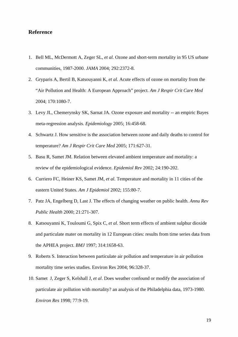
appeared with similar frequency. Fig 1 provides the joint patterns of ozone and temperature on

cardiovascular mortality in the 8 largest communities in the northern region and the 7 largest

communities in the southern region using three-day averages of ozone, temperature and dew

point temperature, respectively. Fig 1 shows that in the northern communities (A to H), ozone

effects increased with temperature except for Oakland (E) and San Jose (G) where ozone

effect changed little with rising temperature, but in the southern communities (I to O), ozone

effects varied only slightly with temperature levels except for Houston (J) and Oklahoma City

(L), where ozone effects were stronger at low temperature than at high temperature.

11

[Fig 1 about here]

To further quantitatively estimate the community-specific ozone-mortality associations

across different temperature levels, we separately fitted the stratification model in each

community (Model B) and then used Bayesian meta-analysis to estimate regional and national

overall ozone effects across different temperature levels. Results show that ozone-mortality

associations were substantially heterogeneous across communities, regions, and temperature

levels. In general, temperature synergistically modified ozone-mortality associations in most

northern, but not obvious in southern communities.

Table 2 provides quantitative Bayesian estimates and 95% posterior intervals (PIs) of

the association between ozone and cardiovascular mortality at both regional and national

levels across three temperature strata where both ozone and temperature are lagged to the

same day, namely current day, lags of one and two day, and three-day averages. Results show

that the associations between ozone and cardiovascular mortality increased with temperature

in the northern areas except for the Upper Midwest, but not obvious in the southern region.

There wereas a significant differences in overall associations between ozone and

cardiovascular mortality for high and low temperature levels in the northern areas. For

example, for per 10-ppb increase in average ozone concentration in the previous three days,

relative risks (RR) of cardiovascular mortality increased 3.49 % (95 % PI: 2.19 %, 4.39 %),

2.46 % (95 % PI: 1.11 %, 3.74 %), 1.05 % (95 % PI: -0.82 %, 2.81 %), 2.77 % (95 % PI:

1.18 %, 4.41 %), 0.57 % (95 % PI: -0.14 %, 1.25 %), 0.76 % (95 % PI: -0.95 %, 2.35 %),

0.57 % (-0.80 %, 1.93 %), 1.68 % (95 % PI: 0.07 %, 3.26 %) in NE, IM, UM, NW, SE, SW,

SC and all 95 communities (National), respectively when temperature was high; 0.43 % (95 %

12

PI: -0.28 %, 1.07 %), 0.47 % (95 % PI: -0.14 %, 1.06 %), 0.33 % (95 % PI: -0.77 %, 1.14 %),

0.35 % (95 % PI: 0.63 %, 1.06 %), 0.39 % (95 % PI: -0.27 %, 1.03 %), 0.42 % (95 % PI: -

0.33 %, 1.17 %), 0.49 % (-0.13 %, 1.10 %), 0.41 % (95 % PI: -0.19 %, 0.93 %) in NE, IM,

UM, NW, SE, SW, SC and National, respectively when temperature was low. The RR

differences between high and low temperatures were 3.06 % (95 % PI: 1.58 %, 4.20 %),

1.99 % (95 % PI: 0.47 %, 3.42 %), 0.72 % (95 % PI: -1.36 %, 2.85 %), 2.42 % (95 % PI:

0.61 %, 4.26 %), 0.18 % (95 % PI: -0.77 %, 1.13 %), 0.34 % (95 % PI: -1.54 %, 2.12 %),

0.08 % (-1.38 %, 1.55 %), 1.27 % (95 % PI: -0.41 %, 2.92 %), respectivelyregion. The

modification was stronger in lag 1 of day than on the current day and lag of two day. Three

day average shows the strongest effect modification.

13

Discussion

This study used two time-series models to explore the associations between ozone and

mortality across temperature levels in 95 large US communities in the summer throughout a

14-year period. Both the bivariate and stratification models indicate that ambient ozone was

associated with cardiovascular mortality and that the associations were substantially

heterogeneous across communities. Results indicate that rising temperature enhanced ozone-

mortality association in the northern region, but such enhancement was not obvious in the

southern region. Overall, the positive association between ozone levels and cardiovascular

mortality was slightly greater at high temperature than at low temperature during the summer

season.

Several previous studies have investigated whether or not temperature modified air

pollution effects. Some studies found evidence that temperature modified the association of air

pollution with human health 8, 9, 11, but others did not.10 For example, Roberts 9 investigated

two US county data between 1987 and 1994 and found that temperature might modify PM10

on mortality (Cook County, IL and Allegheny, PA). Our recent study also indicates that

temperature modified the association between PM10 and morbidity/mortality in Brisbane

between 1996 and 2000.11, 12 This study shows that the modification varied considerately

across communities and climatic regions. Therefore, single or several site studies might

produce conflicting results. However, the joint effects between particulate matter and

temperature are likely to be different from ones between ozone and temperature because ozone

is highly related to temperature in many places.

14

One of our studies examined the effect modification of maximum ozone on the

assessments of associations between maximum temperature and cardiovascular mortality in

the same 95 large U.S. communities and found the associations between temperature and

cardiovascular mortality were different across different ozone levels. Such effect

modifications varied across different regions. In general, maximum ozone modified the

associations between maximum temperature and cardiovascular mortality in the northern

regions, but such effect modification was not obvious in the southern regions.21 The current

study examined the interactive effects between ozone and temperature on cardiovascular

mortality in another perspectives, i.e., effect modification of daily temperature on the

associations between daily ozone and cardiovascular mortality. Both studies found that

temperature and ozone symmetrically modified their associations with cardiovascular

mortality and such modifications were varied across different regions. However, the

magnitudes of effect modifications were different, depending on which variable was

considered as an effect modifier.

Our findings are consistent with previous studies showing that the ozone-mortality

associations substantially varied across seasons or regions.1-3, 12, 17 But these previous studies

did not consider temperature as a modifier in their assessments. For example, Gryparis et al.2

investigated the ozone-mortality relationship in 20 cities in Europe and found the pooled

estimates were weak and not significant for the whole year; nevertheless, mortality increased

by 0.33% (95% confidence interval (CI): 0.17%, 0.52%) and 0.31% (95% CI: 0.17%, 0.52%)

per 10µg/m³ increment in 1-hour ozone and 8-hour ozone during the summer period (April to

September), respectively. They also found geographic differences among the associations –

viz., the effects were higher in southern European cities, compared with northwest and central

eastern regions. Levy et al.3 conducted a meta-analysis and found that the magnitudes of the

15

ozone-mortality relationships substantially differed across seasons (higher in summer). Huang

et al.26 examined the adverse effect of ozone in 19 large NMMAPS communities and found

that a 10-ppb increase in the previous week’s ozone during the summer season (June to

September) was associated with a 1.25 % (95% PI: 0.47%, 2.03%) increase in daily

cardiovascular mortality. Bell et al.1 also conducted a multisite study to estimate overall

relationship between ambient ozone and mortality during the previous days (up to 6 days) in

the same 95 NMMAPS communities as we used here. They found the ozone-mortality

associations were substantially heterogeneous across communities. Nationally, a 10-ppb

increase in ozone over the previous week was associated with 0.64% (95% PI: 0.31%, 0.98%)

and 0.52 % (95% PI: 0.27%, 0.77%) increases for daily cardiovascular and total non-external

mortalities throughout the year, respectively. However, they did not consider seasonal factors,

which might result in overestimates to some extent because more than one-third of the 95

communities, mainly in northern areas, only monitored ozone values during the warm season

(April to October) and ozone effects may be nonlinear.33

This study found that temperature and ozone appeared to have synergistic effects on

CVM. However, biomedical or physiological reasons for such interaction are very complex

because causal ways for both risks are not completely clear and the biological or physiological

reactions are complicated. A number of epidemiological and toxicological studies show that it

is biologically plausible that temperature and ozone modify the effect of each other. Some

experimental studies show that exposure to ozone has significant biological effects on the

respiratory system, including acute and chronic effects.34 Exposure to ozone can result in

injuries to the nasal cavity, trachea and proximal bronchi, and central acinar bronchioles and

alveolar ducts under three primary categories: cellular response, metabolic activity and

physiological changes in respiratory function. 34 It is also known that marked changes in

16

ambient temperature can cause physiological stress and alter a person’s physiological response

to toxic agents.35 Ulmer et al. 36 reported that the average blood pressure in a population

fluctuates with season (more likely via temperature). In elderly persons, the ability to

thermoregulate body temperatures is likely to reduce and sweating thresholds are generally

elevated in comparison with young adults. 37, 38 When body heat production is greater than

necessary to maintain a normal body temperature, blood flow from the body core to the skin

increases, and heat is transferred more rapidly to the external environment. As a result, blood

pressure may increase initially, and heart rates increase subsequently.39 Sharma 40 reported

that some hyperthermia deaths were related to profound brain swelling leading to compression

of vital centres that could responsible for instant death. Therefore, hyperthermia, especially in

susceptible groups, could make them more vulnerable to exposure to toxic agents. Therefore,

high temperature can synergistically modify ozone-mortality associations.

The reasons why the modification effects of temperature on ozone-mortality

associations varied with regions remain largely unknown. We postulate several possible

explanations, but there is lack of supporting evidence so far . Firstly, the relationship between

ozone and temperature varied across different climatic regions (Table 1). In general, ozone

was highly correlated with temperature in the northern region. Therefore, high temperature

and high ozone frequently appeared at the same period, increasing potential joint effects. In

contrast, in the southern region, such correlation varied considerately and was generally

weaker. Because of the weaker or sometimes negative correlation, high temperature and high

ozone only occasionally appeared at the same time and therefore modification will be less

likely to be observed. This difference may partly explain the variation of the effect

modification across the regions. Secondly, other climatic differences may partially explained

the variation of effect modification across different regions. For example, humidity and

17

rainfall are correlated to temperature and ozone. In the southern U.S. region, high humidity

and more cloudy days or rainfall in summer may reduce the ozone generation. These situations

are less happened in the northern U.S. region. Thirdly, physical adaptation of the residents to

exposure to ozone may be another reason for the regional difference. Due to relatively high

levels of ozone and temperature throughout the year in the southern region, residents may

become adapted to high levels of ozone and temperature to some degree. Residents in the

southern may become less sensitive to the variability of ozone and temperature. Some studies

show that after prolonged exposure to ozone, pulmonary functions become adapted, but

inflammation still exists.41, 42 Therefore, the ozone effect changed little with temperature in the

southern region. FinallyThirdly, misclassification of personal exposure to ozone may also

contribute to the variation between different regions. Ozone is very reactive and its

concentrations are much lower indoors than outdoors.2 Due to high temperatures during the

summer in the southern region, air conditioning use might encourage people to stay indoors,

and their personal exposure to ozone may be much lower than the ambient measures. Yet, this

influence may be weaker in the northern region due to relatively lower temperature or

relatively shorter high-temperature periods during the summer. Several studies suggest that the

prevalence of air conditioning is inversely associated with ozone effects.2, 3

In conclusion, this study found that ozone was consistently associated with

cardiovascular mortality and the association was heterogeneous across the geographical

regions of the US. Temperature modified the ozone-cardiovascular mortality association and

the modification varied across different regions. Temperature synergistically modified the

ozone effect on cardiovascular mortality in the northern region, but not obviously so in the

southern region. These findings may have significant implications in the development of

disease control and prevention programs in relation to air pollution and climate change.

18

Acknowledgements

We thank Professors Jonathan Samet, John Hopkins University and Beth Newman,

Queensland University of Technology for their insightful comments. We thank Dr. Peng and

his colleagues, Bloomberg School of Public Health, Johns Hopkins University for making the

database publicly accessible.

19

Reference

1. Bell ML, McDermott A, Zeger SL, et al. Ozone and short-term mortality in 95 US urbane

communities, 1987-2000. JAMA 2004; 292:2372-8.

2. Gryparis A, Bertil B, Katsouyanni K, et al. Acute effects of ozone on mortality from the

“Air Pollution and Health: A European Approach” project. Am J Respir Crit Care Med

2004; 170:1080-7.

3. Levy JL, Chemerynsky SK, Sarnat JA. Ozone exposure and mortality -- an empiric Bayes

meta-regression analysis. Epidemiology 2005; 16:458-68.

4. Schwartz J. How sensitive is the association between ozone and daily deaths to control for

temperature? Am J Respir Crit Care Med 2005; 171:627-31.

5. Basu R, Samet JM. Relation between elevated ambient temperature and mortality: a

review of the epidemiological evidence. Epidemiol Rev 2002; 24:190-202.

6. Curriero FC, Heiner KS, Samet JM, et al. Temperature and mortality in 11 cities of the

eastern United States. Am J Epidemiol 2002; 155:80-7.

7. Patz JA, Engelberg D, Last J. The effects of changing weather on public health. Annu Rev

Public Health 2000; 21:271-307.

8. Katsouyanni K, Touloumi G, Spix C, et al. Short term effects of ambient sulphur dioxide

and particulate mater on mortality in 12 European cities: results from time series data from

the APHEA project. BMJ 1997; 314:1658-63.

9. Roberts S. Interaction between particulate air pollution and temperature in air pollution

mortality time series studies. Environ Res 2004; 96:328-37.

10. Samet J, Zeger S, Kelshall J, et al. Does weather confound or modify the association of

particulate air pollution with mortality? an analysis of the Philadelphia data, 1973-1980.

Environ Res 1998; 77:9-19.

20

11. Ren C, Tong S. Temperature modifies the health effects of particulate matter in Brisbane,

Australia. Int. J. Biometeorol. 2006; 51:87-96.

12. Ren C, Williams GM, Mengersen K, Morawska L, Tong S. Does temperature modify

short-term effect of ozone on total mortality in 60 large eastern US communities? – an

assessment using the NMMAPS data. Environ International 2007; doi:

10.1016/j.envint.2007.10.001

13. Stafoggia M, Schwartz J, Forastiere F, Perucci CA, the SISTI Group. Does Temperature

Modify the Association between Air Pollution and Mortality? A Multicity Case-Crossover

Analysis in Italy. Am J Epidemiol 2008. DOI: 10.1093/aje/kwn074

14. Bateson TF, Schwartz J. Who is sensitive to the effects of particulate air pollution on

mortality: a case-crossover analysis of effect modifiers. Epidemiology 2004; 15:143-9.

15. Jerrett M, Burnett RT, Brook J, et al. Do socioeconomic characteristics modify the short

term association between air pollution and mortality? evidence from a zonal time series in

Hamilton, Canada. J Epidemiol Community Health 2004; 58:31-40.

16. Katsouyanni K, Touloumi G, Samoli E, et al. Confounding and effect modification in the

short-term effects of ambient particles on total mortality: results from 29 European cities

within the APHEA2 project. Epidemiology 2001; 12:521-31.

17. Ito K, De Leon SF, Lippmann M. Association between ozone and daily mortality --

Analysis and meta-analysis. Epidemiology 2005; 16:446-57.

18. Samet JM, Zeger SL, Dominici F, et al. The National Morbidity, Mortality, and Air

Pollution Study, part II: morbidity and mortality from air pollution in the United States.

Cambridge, MA: Health Effects Institute. 2000: 5-79.

19. Internet-based Health & Air Pollution Surveillance System (iHAPSS)

http://www.ihapss.jhsph.edu/ (access May 2nd, 2008).

21

20. Insightful Corporation. S-Plus 6 for Windows Guide to Statistics. Seattle, WA. 2001:380-

434.

21. Ren C, Williams GM, Morawska L, Mengersen K, Tong S. Ozone modifies

associations between temperature and cardiovascular mortality: analysis of the

NMMAPS data. Occup Environ Med 2008; 65:255-260.

22. Ren C Williams MM, Tong S. Does Particulate Matter Modify the Association between

Temperature and Cardiorespiratory Diseases? Environ Health Perspect 2006; 114:1690-

1696.

23. Hastie T, Tibshiranim R. Generalized additive model. New York: Chapman and Hall.

1990:136-73.

24. Daniels MJ, Dominici F, Samet JM., et al. Estimating particulate matter-mortality dose-

response curves and threshold levels: an analysis of daily time-series for the 20 largest US

cities. Am J Epidemiol 2000; 152:397-406.

25. Dominici F, McDermott A, Zeger SL, et al. On the use of generalized additive models in

time-series studies of air pollution and health. Am J Epidemiol 2002; 156:193-203.

26. Huang Y, Dominici F, Bell ML. Bayesian hierarchical distributed lag models fro summer

ozone exposure and cardiorespiratory mortality. Environmetrics 2005; 16:547-62.

27. Dominici F, McDermott A, Hastie T. Improved semiparametric time series models of air

pollution and mortality. J Am Stat Assoc 2004; 99:938-48.

28. Ramsay TO, Burnet RT, Krewski D. The effect of concurvity in generalized additive

models linking mortality to ambient particulate matter. Epidemiology 2003; 14:18-23.

29. McCullagh P, Nelder JA. Generalized linear model (2nd). New York: Chapman and Hall.

1989:98-148.

22

30. Dominici F, Samet JM, Zeger SL. Combining evidence on air pollution and daily mortality

from the 20 largest US cities: a hierarchical modelling strategy. J R Stat Soc [series A]

2000; 163:263-302.

31. Gelman A, Carlin JB, Stern HS, Rubin DB. Bayesian data analysis 2nd. New York: Champ

and Hall, 2004:117-56.

32. Spiegelhaltter D, Thomas A, Best N. WinBUGS version 1.3. Software 2000:1-32.

33. Bell ML, Peng RD, Dominici F. The exposure-response curve for ozone and risk of

mortality and the adequacy of current ozone regulations. Environ Health Perspect 2006;

114:532-6.

34. Paige RC, Plopper CG. Acute and chronic effects of ozone in animal models. In: Holgate

ST, Samet JM, Koren HS and Maynard RL eds. Air Pollution and Health. London:

Academic Press 1999:531-58.

35. Gordon CJ. Role of environmental stress in the physiological response to chemical

toxicants. Environ Res 2003; 92:1-7.

36. Ulmer H, Kelleher C, Diem G, et al. Estimation of seasonal variations in risk factor

profiles and mortality from coronary heart disease. Wien Klin Wochenschr 2004; 116:662-

8.

37. Foster KG, Ellis FT, Dore C, et al. Sweat response in the aged. Age aging 1976; 5:91-101.

38. Kenny WL, Hodson JL. Heat tolerance, thermoregulateion and ageing. Sports Med 1987;

4:446-56.

39. Bouchama A, Knochel JP. Heat stroke. N Engl J Med 2002; 346:1978-88.

40. Sharma HS. Hyperthermia induced brain oedema: current status and future perspectives.

Indian J Med Res 2006; 123:629-52.

41. Folinsbee LJ, Horstman DH, Kehrl HR, et al. Respiratory responses to repeated prolonged

exposure to 0.12 ppm ozone. Am J Respir Crit Care Med 1994; 149:98-105.

23

42. Jörres RA, Holz O, Zachgo W, et al. The effect of repeated ozone exposures on

inflammatory markers in bronchoalveolar lavage fluid and mucosal biopsies. Am J Respir

Crit Care Med 2000; 161:1855-61.

24

Table 1. Summary description for Pearson correlation coefficients between daily maximum

temperature and ozone across different regions during the summer (May to October)

Region1 Number of communities

Correlation coefficients

Mean Minimum 25 Pctl2 Median 75 Pctl Maximum

NE 15 0.618 0.438 0.554 0.642 0.683 0.727

IM 19 0.644 0.589 0.651 0.663 0.695 0.709

UM 7 0.511 0.302 0.439 0.521 0.589 0.644

NW 12 0.399 -0.051 0.368 0.439 0.520 0.620

SE 26 0.279 -0.361 0.031 0.305 0.515 0.623

SW 9 0.218 -0.329 0.061 0.304 0.392 0.540

SC 7 0.350 -0.208 -0.026 0.515 0.728 0.754

1 NE, IM, UM, NW, SE, SW and SC represent the Northeast, Industrial Midwest, Upper Midwest, Northwest, Southeast, Southwest and Southern California, respectively. 2 Pctl denote percentile.

25

Table 2 Percentage changes in daily cardiovascular mortality per 10-ppb increase in ozone across regions and temperature levels during the summer using Bayesian meta-analysis (log relative rate)

Low Temperature

Moderate Temperature

High Temperature

Difference (High-Low)*

Current Day

Northeast 0.63 (0.11,1.20) 0.67 (-0.15, 1.62) 1.23 (0.53, 1.87) 0.60 (-0.27, 1.44)

Industrial Midwest 0.58 (0.07, 1.08) 0.66 (-0.01, 1.39) 1.22 (0.45, 2.10) 0.65 (-0.27, 1.66)

Upper Midwest 0.50 (-0.46, 1.12) 0.43 (-0.80, 1.47) 1.11 (-0.04, 2.32) 0.62 (-0.72, 2.11)

Northwest 0.46 (-0.52, 1.17) 0.22 (-1.05, 1.11) 1.66 (0.51, 3.35) 1.19 (-0.15, 3.04)

Southeast 0.58 (0.01, 1.09) 0.59 ( 0.05, 1.21) 0.62 ( 0.03, 1.20) 0.04 (-0.73, 0.85)

Southwest 0.64 (-0.01, 1.33) 0.26 (-0.75, 1.07) 0.69 (-0.50, 1.72) 0.05 (-1.26, 1.32)

South California 0.63 ( 0.05, 1.25) 0.21 (-0.85, 1.03) 1.04 ( 0.22, 1.92) 0.41 (-0.61, 1.46)

National 0.58 ( 0.07, 1.03) 0.43 (-0.30, 1.08) 1.08 (0.39, 1.89) 0.51 (-0.34, 1.45)

Lag 1

Northeast 0.20 (-0.33, 0.77) 0.42 (-0.10, 0.99) 2.17 (1.15, 2.92) 1.97 (0.82, 2.93)

Industrial Midwest 0.22 (-0.31, 0.80) 0.36 (-0.25, 0.96) 1.83 (0.81, 2.81) 1.60 (0.47, 2.73)

Upper Midwest 0.20 (-0.55, 0.91) 0.41 (-0.35, 1.29) 0.72 (-0.86, 2.31) 0.51 (-1.18, 2.13)

Northwest 0.22 (-0.45, 0.88) 0.45 (-0.29, 1.38) 1.81 (0.39, 3.11) 1.60 (0.04, 3.09)

Southeast 0.16 (-0.39, 0.68) 0.43 (-0.02, 0.93) 0.23 (-0.54, 0.82) 0.07 (-0.73, 0.86)

Southwest 0.26 (-0.41, 1.02) 0.18 (-0.81, 0.85) 0.73 (-0.54, 1.92) 0.47 (-0.98, 1.85)

South California 0.27 (-0.27, 0.92) 0.28 (-0.35, 0.87) 0.07 (-1.04, 1.24) -0.20 (-1.49, 1.08)

National 0.22 (-0.25, 0.72) 0.36 (-0.16, 0.85) 1.08 (-0.09, 2.22) 0.86 (-0.37, 2.07)

Lag 2

Northeast 0.13 (-0.43, 0.79) 0.20 (-0.34, 0.89) 1.20 (0.36, 2.16) 1.07 (-0.01, 2.17)

Industrial Midwest 0.06 (-0.45, 0.59) -0.04 (-0.64, 0.45) 1.15 (0.31, 2.14) 1.09 (0.10, 2.19)

Upper Midwest 0.07 (-0.77, 0.98) 0.10 (-0.65, 0.99) 0.33 (-1.01, 1.34) 0.26 (-1.34, 1.62)

Northwest -0.04 (-0.83, 0.58) 0.00 (-0.83, 0.73) 0.51 (-0.61, 1.43) 0.54 (-0.75, 1.77)

Southeast -0.04 (-0.56, 0.40) 0.01 (-0.47, 0.45) 0.61 (-0.01, 1.25) 0.65 (-0.10, 1.40)

Southwest -0.04 (-0.80, 0.60) -0.20 (-1.27, 0.45) 0.32 (-0.90, 1.26) 0.35 (-1.02, 1.55)

South California 0.05 (-0.54, 0.68) -0.02 (-0.73, 0.55) 0.52 (-0.39, 1.27) 0.47 (-0.64, 1.42)

National 0.03 (0.47, 0.51) 0.01 (-0.53, 0.47) 0.66 (-0.14, 1.37) 0.64 (-0.35, 1.49)

Three – Day Average

Northeast 0.43 (-0.28, 1.07) 0.36 (-0.56, 1.29) 3.49 (2.19, 4.39) 3.06 (1.58, 4.20)

Industrial Midwest 0.47 (-0.14, 1.06) 0.33 (-0.46, 1.12) 2.46 (1.11, 3.74) 1.99 (0.47, 3.42)

Upper Midwest 0.33 (-0.77, 1.14) 0.26 (-0.80, 1.14) 1.05 (-0.82, 2.81) 0.72 (-1.36, 2.85)

Northwest 0.35 (-0.63, 1.06) 0.23 (-0.95, 1.11) 2.77 (1.18, 4.41) 2.42 (0.61, 4.26)

Southeast 0.39 (-0.27, 1.03) 0.39 (-0.22, 1.01) 0.57 (-0.14, 1.25) 0.18 (-0.77, 1.13)

Southwest 0.42 (-0.33, 1.17) 0.05 (-1.28, 0.86) 0.76 (-0.95, 2.35) 0.34 (-1.54, 2.12)

South California 0.49 (-0.13, 1.10) 0.24 (-0.54, 0.89) 0.57 (-0.80, 1.93) 0.08 (-1.38, 1.55)

National 0.41 (-0.19, 0.93) 0.27 (-0.44, 0.87) 1.68 (0.07, 3.26) 1.27 (-0.41, 2.92)

* Differences of the estimates between high temperature level and low temperature levels. The values in the parentheses mean 95% posterior intervals (95% PI).

26

Figure 1 Legend Figure 1 Joint response surfaces of ozone and temperature on cardiovascular mortality in

Chicago(A), Denver(B), Detroit(C), New York(D), Oakland(E), Philadelphia(F), San Jose(G),

Seattle(H) (the 8 largest northern communities) and El Paso(I), Houston(J), Los Angeles(K),

Oklahoma City(L), Phoenix(M), San Diego(N) and Santa Ana/Anaheim(O) (the 7 largest

southern communities) between May and October, 1987-2000.

27

1020

3040

5060

Ozone.Av

20

25

30

35

40

Max.Temperature.Av

-0.1

-0.0

5 0

0.05

0.1

0.15

0.2

Log

Rel

ativ

e R

isk

20

3040

50

Ozone.Av

15

20

25

30

35

Max.Temperature.Av

-0.1-

0.05

00.

050.

10.

150.

20.

25Lo

g R

elat

ive

Ris

k

20

30

40

50

Ozone.Av20

25

30

35

40

45

Max.Temperature.Av

-0.1

5-0

.1-0

.05

00.

050.

10.

15Lo

g R

elat

ive

Ris

k

1020

3040

5060

Ozone.Av

22

24

26

28

30

32

34

Max.Temperature.Av

-0.1

5-0

.1-0

.05

00.

050.

10.

15Lo

g R

elat

ive

Ris

k

1020

3040

50

Ozone.Av20

25

30

35

Max.Temperature.Av

-0.0

5 0

0.05

0.1

0.15

0.2

0.25

0.3

Log

Rel

ativ

e R

isk

1020

3040

5060

Ozone.Av20

25

30

35

40

Max.Temperature.Av

-0.0

8-0.0

6-0.0

4-0.0

2 0

0.02

0.04

0.06

Log

Rel

ativ

e R

isk

20

30

40

50

Ozone.Av

15

20

25

30

35

40

Max.Temperature.Av

-0.3

-0.2

-0.1

00.

10.

20.

30.

4Lo

g R

elat

ive

Ris

k

10

20

3040

50

Ozone.Av

10

15

20

25

30

35

Max.Temperature.Av

-0.1

00.

10.

20.

3Lo

g R

elat

ive

Ris

k

10

20

30

40

Ozone.Av

15

20

25

30

35

40

Max.Temperature.Av

-0.0

5 0

0.05

0.1

0.15

0.2

Log

Rel

ativ

e R

isk

0

20

40

60

Ozone.Av

10

15

20

25

30

35

Max.Temperature.Av

-0.2

-0.1

00.

10.

20.

3Lo

g R

elat

ive

Ris

k

1015

2025

3035

40

Ozone.Av

15

20

25

30

35

40

Max.Temperature.Av

-0.1

5-0.

1-0.

05 0

0.05

0.1

0.15

Log

Rel

ativ

e R

isk

1020

3040

5060

Ozone.Av

10

15

20

25

30

35

Max.Temperature.Av

-0.1

00.

10.

20.

30.

4Lo

g R

elat

ive

Ris

k

1020

3040

5060

Ozone.Av

5

10

15

20

25

30

35

Max.Temperature.Av

-0.1

00.

10.

20.

30.

4Lo

g R

elat

ive

Ris

k

10

20

30

40

Ozone.Av10

20

30

40

Max.Temperature.Av

-0.1

-0.0

5 0

0.05

0.1

0.15

0.2

Log

Rel

ativ

e R

isk

1020

3040

50

Ozone.Av10

20

30Max.Temperature.Av

-0.1

00.

10.

20.

30.

4Lo

g R

elat

ive

Ris

k A B C D E F G H I J K L M N O Figure 1