1

Temperature dependence of nitrogen-vacancy center

ensembles in diamond based on an optical fiber

Ke-Chen Ouyang1,2, Zheng Wang2,3, Li Xing2, Xiao-Juan Feng2,, Jin-Tao Zhang2, Cheng Ren1, Xing-

Tuan Yang1

1Institute of Nuclear and New Energy Technology, Tsinghua University, Beijing 100084, China

2National Institute of Metrology, Beijing 100029, China

3Department of Precision Instrument, Tsinghua University, Beijing 100084, China

The nitrogen-vacancy (NV) centers in diamond sensing has been considered to be a promising micro-

nano scale thermometer due to its high stability, good temperature resolution and integration. In this work,

we fabricated the sensing core by attaching a diamond plate containing NV centers to the section of a

cut-off multi-mode fiber. Then we measured the zero-field splitting parameter (D) of NV center

ensembles using continuous-wave optical detected magnetic resonance (CW-ODMR) technique. A

home-made thermostatic system and two calibrated platinum resistance thermometers were applied for

reference temperature measurement. The effects from preparation time and count time in the pulse

sequence, laser power, microwave power, and microwave frequency step were investigated. Moreover,

the experimental D and T from 298.15 K to 383.15 K was obtained with the standard uncertainty of u(D)

= (3.62268~8.54464) × 10-5 GHz and u(T) = (0.013~ 0.311) K. The experimental results are well

consistent with the work of Toyli, et al. (Toyli, et al., 2012) using the similar diamond sample. The

extrapolation for D-T at 0 K and 700 K also agree with other references, and meanwhile dD/dT varies

with temperature. Finally, comparing the D-T relationship measured by different research groups, we can

know that the NV concentration resulting in different electron density and manufacturing procedure

resulting in different thermal expansion would lead to different D-T relationship. It is worthy to continue

further comprehensive research especially from the metrological point of view to develop NV center as

a practical and accurate micro-nano scale thermometry.

Ⅰ. INTRODUCTION

The nitrogen-vacancy (NV) center in diamond has been applied to detecting several physical

quantity including magnetic field [1,2], electric field [3,4], pressure [5,6], and temperature [7-9]

fengxj@nim.ac.cn

2

with high accuracy and short response time. The diamond thermometer has been applied for nano-

scale temperature measurement, such as in cells [10,11], in organisms [12,13], on chips [14,15], et

al. The electron spin of NV centers can be polarized by laser and the spin state can be manipulated

by microwave of certain frequency. Thus, the NV center have ultra-high sensitivity to measure

temperature by the variety of zero-field splitting energy (D) [8,10,15]. Due to the nano-scale of NV

centers and the physical stability of diamond, the thermometry has advantages on high resolution

and robustness [7,16]. The active control of laser polarization and microwave manipulation enables

it to be resistive to ambient environmental by encoding certain sequences of laser and microwave

[17,18]. Recently, the technology for optical fiber probe coupled with NV centers makes it have the

potential of integration [19-21,15]. High-resolution temperature measurement is based on NV

centers with an accurate calibration of D-T relationship. However, the parameters of reference

temperature, laser, microwave and diamond sample have influence on the acquisition of the D-T

relationship. Therefore, it is significant to improve the reliability of calibrating the D-T relation.

Several groups have researched on the relationship between D and T. According to Ref. [22], the

temperature dependence of NV centers magnetic resonance from 280 K~330 K was studied, and the

relation of dD/dT = -74.2(7) kHz/K was got in 2010. Besides, the group used different diamond

samples for experimental and obtained different values of dD/dT. A fifth-order polynomial relation

of D and T from 5.6 K to 295 K and a third-order polynomial relation from room temperature to

700 K were obtained in 2011 and 2012, respectively [23,14]. In 2014, another second-order

polynomial relation of D-T from 300 K to 600 K was worked out and the result was found in good

consistency with that in Ref. [9,14]. In 2018, a similar rate of frequency shift over temperature

change with that in Ref. 22, which is equal to -74.2 kHz/K, was acquired from 297 K to 333 K [24].

In conclusion, present D-T relations vary with different groups and it is necessary to carry on careful

experiments to provide reference for the application of NV centers thermometry.

In this work, to obtain a good thermal equilibrium between the NV center and reference

thermometers, we fabricated a sensor based on optical fiber and calibrated it in a close thermostatic

cavity. We attached the diamond sample with NV centers to the section of a cut-off multi-mode

optical fiber and built up a continuous-wave optical detected magnetic resonance (CW-ODMR)

system and a home-made thermostatic system. Then we determined the optimal combination of

ODMR experimental parameters by several groups of tests, based on which we carried out the

3

ODMR experiments from 298.15 K to 383.15 K with a step of 5 K. The corresponding zero-field

splitting parameter(D) in every temperature value(T) was obtained by fitting the spectra data with

the most appropriate function. Accordingly, we attained the relationship between D and T in the

temperature range from 298.15 K to 383.15 K and analyzed uncertainty budget sources in detail.

Finally, we compared the results with those of other research groups to demonstrate the consistency

and discussed the connection between different samples and D-T relationship.

Ⅱ. EXPERIMENTAL SETUP AND MEASUREMENT

PROCEDURE

A. Principle of temperature measurement by NV centers

The physical quantity that can be detected by the NV center is determined by the Hamiltonian,

which is expressed as [8]

HNV = DSz2 + g

sμ

BB∙S + SAI (1)

where D is the zero-field splitting parameter between the sublevels ms=0 and ms=±1. S represents

spin angular momentum with its component Sx, Sy, Sz in three axis, respectively. gs is dimensionless

magnetic moment (Landé g-factor) and μB is Bohr magneton. B stands for vector external magnetic

field. �� is the hyperfine tensor and I is the spin operation of nitrogen nucleus. The first item of of

the right-side of the equation (1) reflects the influence from temperature, the second item reflects

the influence by magnetic field on the fine structure of NV center, while the third one reflects the

influence by strain and electric field.

The influence by temperature on NV center is estimated by the variation of the zero-field splitting

parameter D. The ground state of NV center is spin-triplet with the sublevels ms = 0 and ms =±1.

The sub-levels ms = ±1 are degenerated when there is no external magnetic field applied. Between

the sublevels ms = 0 and ms =±1 exists a splitting called the zero-field splitting, which can be

represented by the parameter D. The value of D changes with the temperature of the spot where the

NV center locates. Thus, we can measure the value of D by ODMR technique and then obtain the

corresponding temperature T by calibrating the relationship between D and T.

According to the NV- molecular model, the expression of D can be yielded as [25]

4

D ≈ Cη2 ⟨1

r123 -

3z122

r125 ⟩ (2)

where C is the spin-spin interaction constant, ri = xix + yiy + zi z is the position of the ith electron,

of which r12 = |r2-r1|, z12 = z2-z1, η is the electron density. The value of D is dependent of η and

⟨1

r123 -

3z122

r125 ⟩, which represents the interaction between the dangling 𝑠𝑝3 electron densities of the two

carbon atoms. Rise in temperature will cause local thermal expansion in diamond lattice, and then

increase the value of r12. Thus, the value of D will correspondingly decrease with η unchanged and

the variety of D can be observed by measuring the ODMR spectrum.

B. Experimental setup

The experimental setup is based on CW-ODMR technique and an optical fiber thermometer

coupled with NV center ensembles to realize highly reliable temperature measurement. The

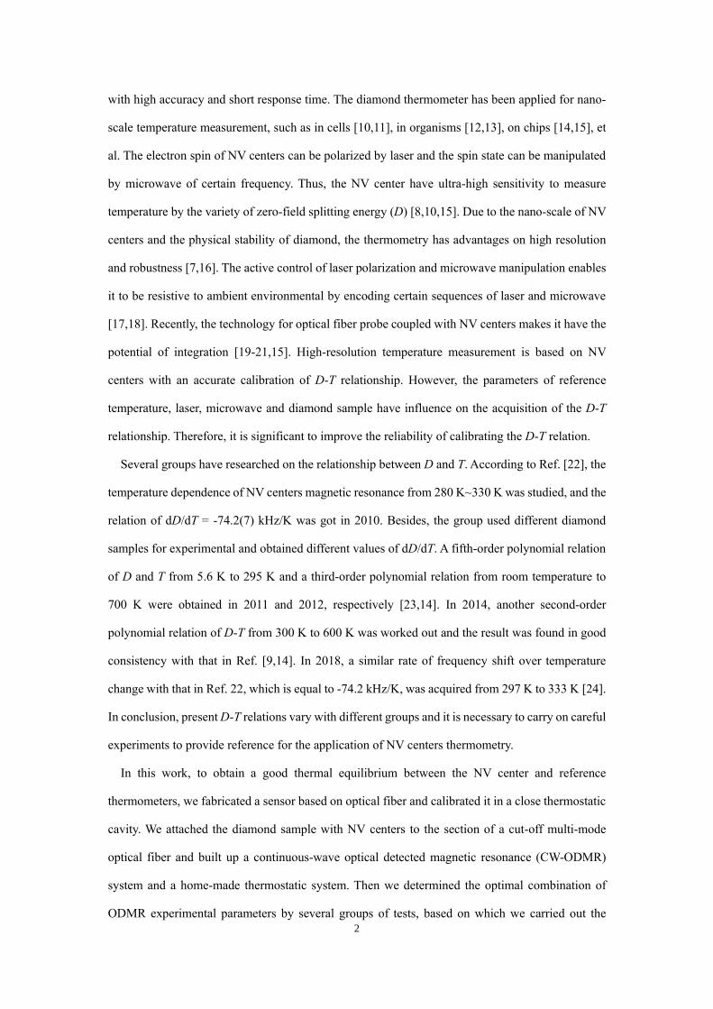
experimental system, as showed in Fig. 1, includes five parts: the laser polarization system, the

sensing core, the microwave manipulation system, the fluorescence detecting system, and the

thermostatic system. In the ODMR experiment, a polarization beam at 532 nm is emitted by a laser

(CNI-MGL-Ⅲ-532-200mW) and modulated by an acousto-optic modulator (AOM, AODR

1080AF-DIF0-1.0 from Gooch & Housego), which can polarize the electron spins of NV centers.

The microwave manipulation system is applied to provide sufficiently high power microwave for

NV centers to change the spin states, in which an amplifier (ZHL-16W-43-S+ from Mini-Circuits)

is set to amplify the microwave from the microwave generator (SMIQ 06B from Rohde & Schwarz)

and a RF switch (ZASWA-2-50DRA+ from Mini-Circuits) controls the on-off of the microwave

signal. Fluorescence released by the polarized NV centers can be detected by a single photon count

modulator (SPCM, SPCM-AQRH-11-FC from Excelitas). Then the data is collected by a data

acquisition (DAQ, USB6363 from National Instrument) connected with the SPCM. To better control

the laser, the microwave and the readout to switch on or off, the AOM, the RF Switch and the DAQ

are all connected with a pulse generator (PBESR-PRO-500-PCI from SpinCore), which is inserted

in the computer. Finally, the CW-ODMR spectra can be measured by frequency sweeping.

5

FIG. 1. The schematic diagram of the experimental system. AOM: acousto-optic modulator. SPCM: single photon

count modulator. DAQ: data acquisition.

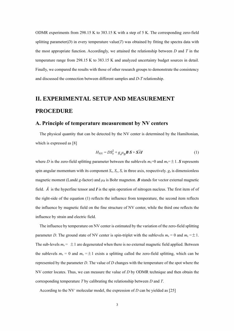
The sensing core consists of a multi-mode optical fiber, a diamond plate (Element Six EL SC

Plate, 2.0 mm × 2.0 mm × 0.5 mm, [Ns0] <5 ppb) and a copper wire (60 μm in diameter), as shown

in Fig. 2. The fiber is 1 m in length and we cut it in half with a ceramic fiber scribe. Then we attached

the diamond plate to the section of the fiber with UV-curing optical adhesives. Next, we stuck the

copper wire to the plate using the same glue and bond it to the fiber with adhesive tape and raw

material belt. The wire has two free ends, one of which is connected with a high power amplifier

through a coaxial cable while the other is connected with a resistance by another cable to absorb the

microwave.

FIG. 2. The schematic diagram and the picture of the sensor.

To form a temperature field with high stability and homogeneity, we set up a close thermostatic

cavity, which is comprised of a self-designed temperature controller, a heater, a DC power supply,

a millikelvin thermometer (MKT 50 from Anton Paar), two platinum resistance thermometers (Pt-

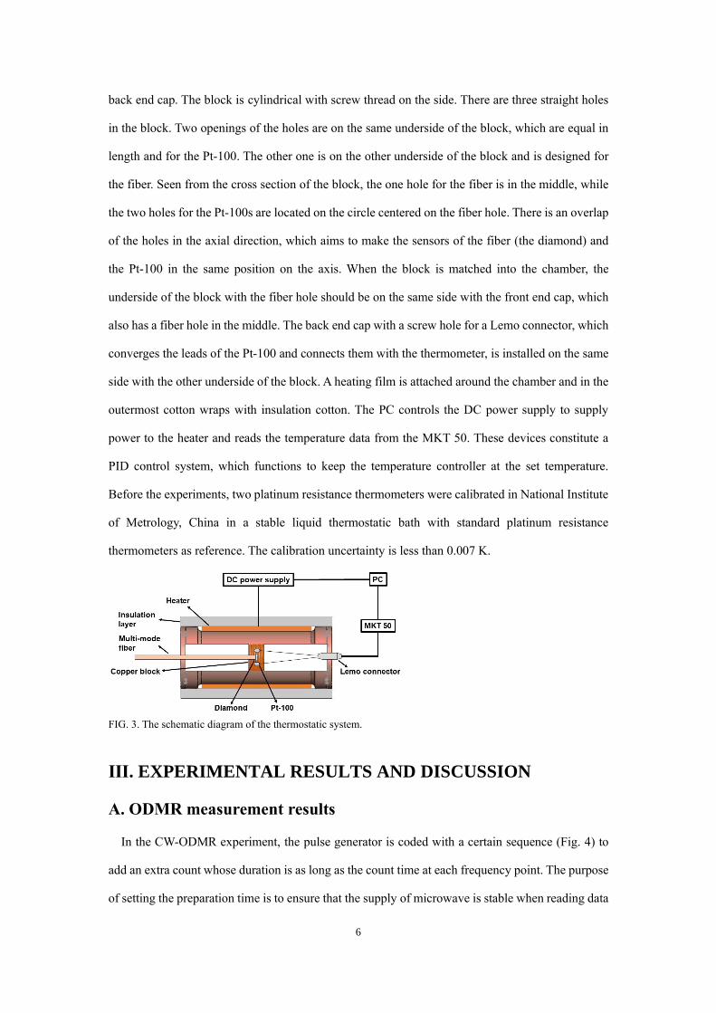
100) and a PC. The schematic diagram is illustrated in Fig. 3. The main body of the system is the

temperature controller, which includes a cylindrical chamber, a copper block, a front end cap and a

6

back end cap. The block is cylindrical with screw thread on the side. There are three straight holes

in the block. Two openings of the holes are on the same underside of the block, which are equal in

length and for the Pt-100. The other one is on the other underside of the block and is designed for

the fiber. Seen from the cross section of the block, the one hole for the fiber is in the middle, while

the two holes for the Pt-100s are located on the circle centered on the fiber hole. There is an overlap

of the holes in the axial direction, which aims to make the sensors of the fiber (the diamond) and

the Pt-100 in the same position on the axis. When the block is matched into the chamber, the

underside of the block with the fiber hole should be on the same side with the front end cap, which

also has a fiber hole in the middle. The back end cap with a screw hole for a Lemo connector, which

converges the leads of the Pt-100 and connects them with the thermometer, is installed on the same

side with the other underside of the block. A heating film is attached around the chamber and in the

outermost cotton wraps with insulation cotton. The PC controls the DC power supply to supply

power to the heater and reads the temperature data from the MKT 50. These devices constitute a

PID control system, which functions to keep the temperature controller at the set temperature.

Before the experiments, two platinum resistance thermometers were calibrated in National Institute

of Metrology, China in a stable liquid thermostatic bath with standard platinum resistance

thermometers as reference. The calibration uncertainty is less than 0.007 K.

FIG. 3. The schematic diagram of the thermostatic system.

Ⅲ. EXPERIMENTAL RESULTS AND DISCUSSION

A. ODMR measurement results

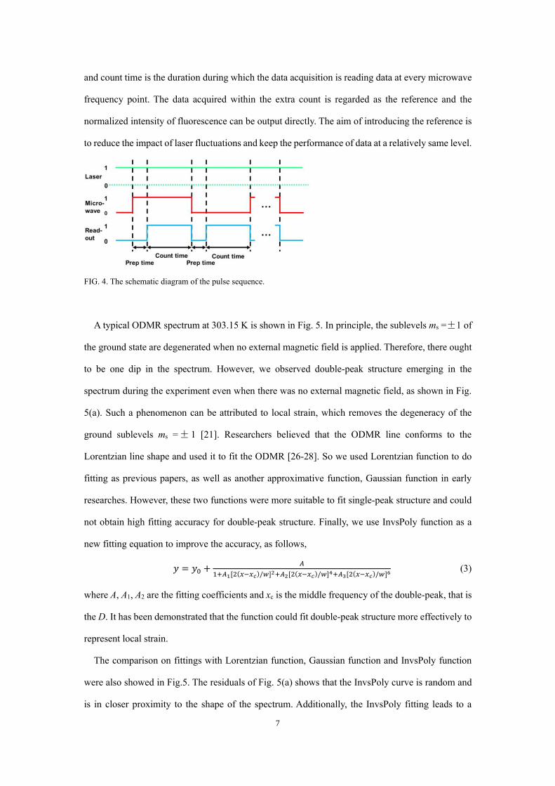
In the CW-ODMR experiment, the pulse generator is coded with a certain sequence (Fig. 4) to

add an extra count whose duration is as long as the count time at each frequency point. The purpose

of setting the preparation time is to ensure that the supply of microwave is stable when reading data

7

and count time is the duration during which the data acquisition is reading data at every microwave

frequency point. The data acquired within the extra count is regarded as the reference and the

normalized intensity of fluorescence can be output directly. The aim of introducing the reference is

to reduce the impact of laser fluctuations and keep the performance of data at a relatively same level.

FIG. 4. The schematic diagram of the pulse sequence.

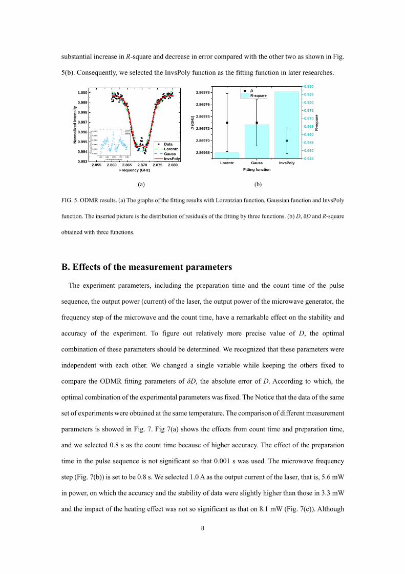
A typical ODMR spectrum at 303.15 K is shown in Fig. 5. In principle, the sublevels ms =±1 of

the ground state are degenerated when no external magnetic field is applied. Therefore, there ought

to be one dip in the spectrum. However, we observed double-peak structure emerging in the

spectrum during the experiment even when there was no external magnetic field, as shown in Fig.

5(a). Such a phenomenon can be attributed to local strain, which removes the degeneracy of the

ground sublevels ms =±1 [21]. Researchers believed that the ODMR line conforms to the

Lorentzian line shape and used it to fit the ODMR [26-28]. So we used Lorentzian function to do

fitting as previous papers, as well as another approximative function, Gaussian function in early

researches. However, these two functions were more suitable to fit single-peak structure and could

not obtain high fitting accuracy for double-peak structure. Finally, we use InvsPoly function as a

new fitting equation to improve the accuracy, as follows,

𝑦 = 𝑦0 +𝐴

1+𝐴1[2(𝑥−𝑥𝑐)/𝑤]2+𝐴2[2(𝑥−𝑥𝑐)/𝑤]4+𝐴3[2(𝑥−𝑥𝑐)/𝑤]6 (3)

where A, A1, A2 are the fitting coefficients and xc is the middle frequency of the double-peak, that is

the D. It has been demonstrated that the function could fit double-peak structure more effectively to

represent local strain.

The comparison on fittings with Lorentzian function, Gaussian function and InvsPoly function

were also showed in Fig.5. The residuals of Fig. 5(a) shows that the InvsPoly curve is random and

is in closer proximity to the shape of the spectrum. Additionally, the InvsPoly fitting leads to a

8

substantial increase in R-square and decrease in error compared with the other two as shown in Fig.

5(b). Consequently, we selected the InvsPoly function as the fitting function in later researches.

(a) (b)

FIG. 5. ODMR results. (a) The graphs of the fitting results with Lorentzian function, Gaussian function and InvsPoly

function. The inserted picture is the distribution of residuals of the fitting by three functions. (b) D, δD and R-square

obtained with three functions.

B. Effects of the measurement parameters

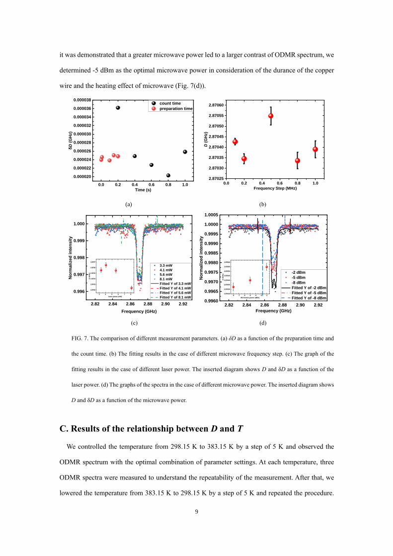
The experiment parameters, including the preparation time and the count time of the pulse

sequence, the output power (current) of the laser, the output power of the microwave generator, the

frequency step of the microwave and the count time, have a remarkable effect on the stability and

accuracy of the experiment. To figure out relatively more precise value of D, the optimal

combination of these parameters should be determined. We recognized that these parameters were

independent with each other. We changed a single variable while keeping the others fixed to

compare the ODMR fitting parameters of δD, the absolute error of D. According to which, the

optimal combination of the experimental parameters was fixed. The Notice that the data of the same

set of experiments were obtained at the same temperature. The comparison of different measurement

parameters is showed in Fig. 7. Fig 7(a) shows the effects from count time and preparation time,

and we selected 0.8 s as the count time because of higher accuracy. The effect of the preparation

time in the pulse sequence is not significant so that 0.001 s was used. The microwave frequency

step (Fig. 7(b)) is set to be 0.8 s. We selected 1.0 A as the output current of the laser, that is, 5.6 mW

in power, on which the accuracy and the stability of data were slightly higher than those in 3.3 mW

and the impact of the heating effect was not so significant as that on 8.1 mW (Fig. 7(c)). Although

2.855 2.860 2.865 2.870 2.875 2.8800.993

0.994

0.995

0.996

0.997

0.998

0.999

1.000

2.860 2.865 2.870 2.875 2.880

-0.0010

-0.0005

0.0000

0.0005

0.0010

0.0015 Lorentz

Guass

InsPoly

Re

sid

uals

of

No

rma

lized

in

ten

sit

y

X of Normalized intensity

Data

Lorentz

Gauss

InvsPoly

No

rmalized

in

ten

sit

y

Frequency (GHz)

Lorentz Gauss InvsPoly

2.86968

2.86970

2.86972

2.86974

2.86976

2.86978 D

R-square

Fitting function

D (

GH

z)

0.945

0.950

0.955

0.960

0.965

0.970

0.975

0.980

0.985

0.990

R-s

qu

are

9

it was demonstrated that a greater microwave power led to a larger contrast of ODMR spectrum, we

determined -5 dBm as the optimal microwave power in consideration of the durance of the copper

wire and the heating effect of microwave (Fig. 7(d)).

(a) (b)

(c) (d)

FIG. 7. The comparison of different measurement parameters. (a) δD as a function of the preparation time and

the count time. (b) The fitting results in the case of different microwave frequency step. (c) The graph of the

fitting results in the case of different laser power. The inserted diagram shows D and δD as a function of the

laser power. (d) The graphs of the spectra in the case of different microwave power. The inserted diagram shows

D and δD as a function of the microwave power.

C. Results of the relationship between D and T

We controlled the temperature from 298.15 K to 383.15 K by a step of 5 K and observed the

ODMR spectrum with the optimal combination of parameter settings. At each temperature, three

ODMR spectra were measured to understand the repeatability of the measurement. After that, we

lowered the temperature from 383.15 K to 298.15 K by a step of 5 K and repeated the procedure.

0.0 0.2 0.4 0.6 0.8 1.0

0.000020

0.000022

0.000024

0.000026

0.000028

0.000030

0.000032

0.000034

0.000036

0.000038 count time

preparation time

δD

(G

Hz)

Time (s)

0.0 0.2 0.4 0.6 0.8 1.02.87025

2.87030

2.87035

2.87040

2.87045

2.87050

2.87055

2.87060

D (

GH

z)

Frequency Step (MHz)

2.82 2.84 2.86 2.88 2.90 2.92

0.996

0.997

0.998

0.999

1.000

3 4 5 6 7 8

2.8702

2.8703

2.8704

2.8705

2.8706

2.8707

D (

GH

z)

Laser power (mW)

3.3 mW

4.1 mW

5.6 mW

8.1 mW

Fitted Y of 3.3 mW

Fitted Y of 4.1 mW

Fitted Y of 5.6 mW

Fitted Y of 8.1 mW

No

rma

lized

in

ten

sit

y

Frequency (GHz)

2.82 2.84 2.86 2.88 2.90 2.920.9960

0.9965

0.9970

0.9975

0.9980

0.9985

0.9990

0.9995

1.0000

1.0005

-8 -7 -6 -5 -4 -3 -22.87025

2.87030

2.87035

2.87040

2.87045

2.87050

2.87055

2.87060

D (

GH

z)

Microwave power (dBm)

-2 dBm

-5 dBm

-8 dBm

Fitted Y of -2 dBm

Fitted Y of -5 dBm

Fitted Y of -8 dBm

No

rmalized

in

ten

sit

y

Frequency (GHz)

10

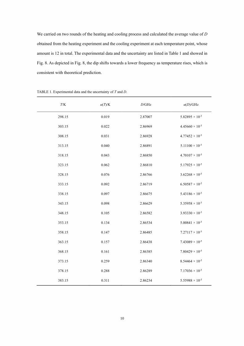
We carried on two rounds of the heating and cooling process and calculated the average value of D

obtained from the heating experiment and the cooling experiment at each temperature point, whose

amount is 12 in total. The experimental data and the uncertainty are listed in Table 1 and showed in

Fig. 8. As depicted in Fig. 8, the dip shifts towards a lower frequency as temperature rises, which is

consistent with theoretical prediction.

TABLE 1. Experimental data and the uncertainty of T and D.

T/K u(T)/K D/GHz u(D)/GHz

298.15

303.15

308.15

313.15

318.15

323.15

328.15

333.15

338.15

343.15

348.15

353.15

358.15

363.15

368.15

373.15

378.15

383.15

0.019

0.022

0.031

0.040

0.043

0.062

0.076

0.092

0.097

0.098

0.105

0.134

0.147

0.157

0.161

0.259

0.288

0.311

2.87007

2.86969

2.86928

2.86891

2.86850

2.86810

2.86766

2.86719

2.86675

2.86629

2.86582

2.86534

2.86485

2.86438

2.86385

2.86340

2.86289

2.86234

5.82895 × 10-5

4.45660 × 10-5

4.77452 × 10-5

5.11100 × 10-5

4.70107 × 10-5

5.17925 × 10-5

3.62268 × 10-5

6.50587 × 10-5

5.43186 × 10-5

5.35958 × 10-5

3.93330 × 10-5

5.00841 × 10-5

7.27117 × 10-5

7.43089 × 10-5

7.80429 × 10-5

8.54464 × 10-5

7.17036 × 10-5

5.55988 × 10-5

11

(a) (b)

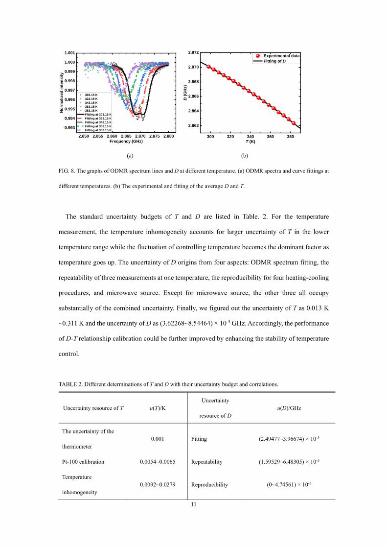
FIG. 8. The graphs of ODMR spectrum lines and D at different temperature. (a) ODMR spectra and curve fittings at

different temperatures. (b) The experimental and fitting of the average D and T.

The standard uncertainty budgets of T and D are listed in Table. 2. For the temperature

measurement, the temperature inhomogeneity accounts for larger uncertainty of T in the lower

temperature range while the fluctuation of controlling temperature becomes the dominant factor as

temperature goes up. The uncertainty of D origins from four aspects: ODMR spectrum fitting, the

repeatability of three measurements at one temperature, the reproducibility for four heating-cooling

procedures, and microwave source. Except for microwave source, the other three all occupy

substantially of the combined uncertainty. Finally, we figured out the uncertainty of T as 0.013 K

~0.311 K and the uncertainty of D as (3.62268~8.54464) × 10-5 GHz. Accordingly, the performance

of D-T relationship calibration could be further improved by enhancing the stability of temperature

control.

TABLE 2. Different determinations of T and D with their uncertainty budget and correlations.

Uncertainty resource of T u(T)/K

Uncertainty

resource of D

u(D)/GHz

The uncertainty of the

thermometer

0.001 Fitting (2.49477~3.96674) × 10-5

Pt-100 calibration 0.0054~0.0065 Repeatability (1.59529~6.48305) × 10-5

Temperature

inhomogeneity

0.0092~0.0279 Reproducibility (0~4.74561) × 10-5

2.850 2.855 2.860 2.865 2.870 2.875 2.880

0.993

0.994

0.995

0.996

0.997

0.998

0.999

1.000

1.001

303.15 K

323.15 K

343.15 K

363.15 K

383.15 K

Fitting at 303.15 K

Fitting at 323.15 K

Fitting at 343.15 K

Fitting at 363.15 K

Fitting at 383.15 K

No

rma

lized

in

ten

sit

y

Frequency (GHz)300 320 340 360 380

2.862

2.864

2.866

2.868

2.870

2.872 Experimental data

Fitting of D

D (

GH

z)

T (K)

12

Temperature fluctuation 0.0065~0.3092

Frequency

uncertainty of

microwave source

2.9 × 10-5

Combined uncertainty/K 0.013~0.311

Combined

uncertainty/GHz

(3.62268~8.54464) × 10-5

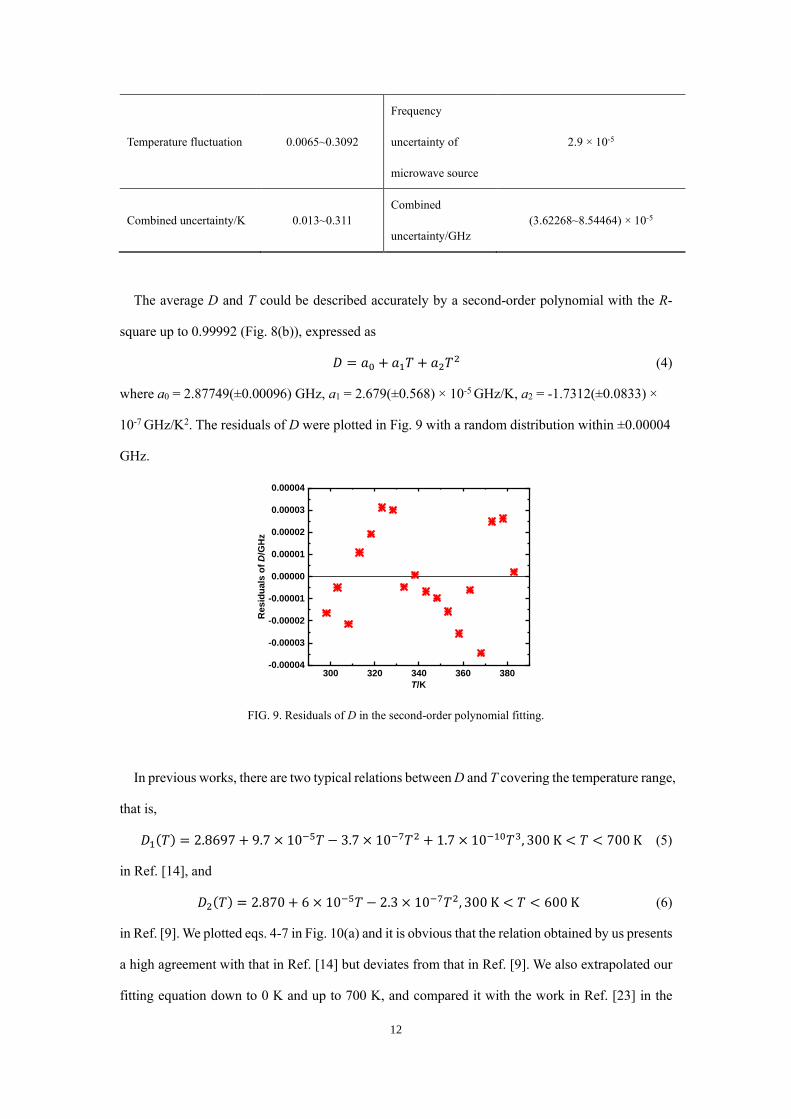
The average D and T could be described accurately by a second-order polynomial with the R-

square up to 0.99992 (Fig. 8(b)), expressed as

𝐷 = 𝑎0 + 𝑎1𝑇 + 𝑎2𝑇2 (4)

where a0 = 2.87749(±0.00096) GHz, a1 = 2.679(±0.568) × 10-5 GHz/K, a2 = -1.7312(±0.0833) ×

10-7 GHz/K2. The residuals of D were plotted in Fig. 9 with a random distribution within ±0.00004

GHz.

FIG. 9. Residuals of D in the second-order polynomial fitting.

In previous works, there are two typical relations between D and T covering the temperature range,

that is,

𝐷1(𝑇) = 2.8697 + 9.7 × 10−5𝑇 − 3.7 × 10−7𝑇2 + 1.7 × 10−10𝑇3, 300 K < 𝑇 < 700 K (5)

in Ref. [14], and

𝐷2(𝑇) = 2.870 + 6 × 10−5𝑇 − 2.3 × 10−7𝑇2, 300 K < 𝑇 < 600 K (6)

in Ref. [9]. We plotted eqs. 4-7 in Fig. 10(a) and it is obvious that the relation obtained by us presents

a high agreement with that in Ref. [14] but deviates from that in Ref. [9]. We also extrapolated our

fitting equation down to 0 K and up to 700 K, and compared it with the work in Ref. [23] in the

300 320 340 360 380-0.00004

-0.00003

-0.00002

-0.00001

0.00000

0.00001

0.00002

0.00003

0.00004

Re

sid

uals

of

D/G

Hz

T/K

13

temperature range from 5.6 K to 295 K,

𝐷3(𝑇) = 2.87771 − 4.625 × 10−6𝑇 + 1.067 × 10−7𝑇2 − 9.325 × 10−10𝑇3

+1.739 × 10−12𝑇4 − 1.838 × 10−15𝑇5 (7)

The extrapolation of present D-T equation to high temperature agrees well with that in Ref. [14] and

the extrapolation to low temperature agrees well with the relation obtained in Ref. [23], which

proves the reliability of the experimental data.

The first order differential of the relationship between D and T from this work is

d𝐷

d𝑇= 2.679 × 10−5 − 3.4624 × 10−7𝑇 (8)

The comparison of dD/dT as a function of T in several references, including Ref. [14], Ref. [9],

Ref. [24]. and Ref. [22] and this work is plotted in Fig. 10(b). To figure out the origin of consistency

and deviation between different researches, we compared the experimental conditions of different

works in Table 3. CW-ODMR was applied in all the references. The relationship of D-T in Ref. [14],

Ref. [23] and this work, are highly consistent even in extrapolated range because of using similar

samples. The difference between the trends of dD/dT origins from two aspects: the discrepancy

between the manufacturing technology and NV concentration of the diamond samples, which can

be explained by eq. 2. At the same temperature, the electron density η increases with the increasing

NV concentration, and the parameters involved in the formula, ⟨1

r123 -

3z122

r125 ⟩, which are regarded as the

internal attribution of NV centers microscopically, remained unchanged. Therefore, lower

concentration of NV centers will lead to a smaller value of D at the same temperature, which is

proved by the deviation of the result in Ref. [9] from the others in Fig. 10(a). When temperature

varies, the distance between NV lattice changed so that the value of ⟨1

r123 -

3z122

r125 ⟩ changes results in a

dependence of D on T. The results from present work and Ref. [14] and Ref. [9] confirm that dD/dT

varies with temperature. Therefore, it is necessary to calibrate the value of dD/dT at different

temperatures to obtain reliable measurement results. Furthermore, for the application of the NV

centers thermometry, it is necessary to check the samples’ properties when using a reference’s D-T

relationship.

14

(a) (b)

FIG. 10. (a) Comparison of four D-T relationship curves obtained in Ref. [14], Ref. [9], Ref. [23], and this work. (b)

Comparison of d𝐷/d𝑇of the works from different references.

TABLE 3. Comparison of the technique details between different measurements.

Reference Diamond type Manufacturer Manufacturing

technology NV concentration

Ref. [14] Single-crystal

diamond /

CVD (Chemical

Vapor Deposition) [𝑁𝑆

0] < 5 ppb

Ref. [9]

Type Ⅰb HPHT

nano-diamond

crystals

/

HPHT (High

Pressure and High

Temperature)

15 NV- centers each

Ref. [24] Single-crystal

diamond Element-Six CVD [𝑁𝑆

0] < 5 ppb

Ref. [23] Single-crystal

diamond Element-Six CVD [N]<1 ppm

Ref. [22] Single-crystal

diamond /

S3: CVD; S2, S5, S8:

HPHT

S2: [NV-]=16 ppm;

S3: [NV-]=10 ppb;

S5: [NV-]=12 ppm;

S8: [NV-]=0.3 ppm

This work Single-crystal

diamond Element-Six CVD

[𝑁𝑆0] < 5 ppb , [NV]<0.03

ppb

Ⅳ. CONCLUSION

To realize a reliable relationship between the zero-field splitting parameter D and temperature T

for ensemble NV centers in diamond, we fabricated an optical fiber sensor coupled with NV centers,

built up a CW-ODMR experimental system and a close thermostatic chamber for better thermal

equilibrium. The measurement parameters and fitting function for the ODMR spectrum were

compared and optimized. The ODMR experiments in the temperature range from 298.15 K to

383.15 K were carried out in four thermal circulates with a result of standard uncertainty of u(D)=

(3.62268~8.54464) × 10-5 GHz and u(T)= (0.013~ 0.311) K. The experimental D-T was fitted using

0 100 200 300 400 500 600 7002.81

2.82

2.83

2.84

2.85

2.86

2.87

2.88

D1, Toyli, 2012

D2, Plakhotnik, 2014

D3, Chen, 2011

Experimental data, this work

Fitting, this work

D (

GH

z)

T (K)

280 300 320 340 360 380-120

-115

-110

-105

-100

-95

-90

-85

-80

-75

-70

dD

/dT

(kH

z/K

)

T (K)

Toyli, 2012

Plakhotnik, 2014

Sunuk Choe, 2018

S2, Acosta, 2010

S3, Acosta, 2010

S5, Acosta, 2010

S8, Acosta, 2010

This work

15

a second-order polynomial correlation with a maximal residual of 0.00004 GHz. We extrapolated

the relationship of present D-T to a wider temperature range from 0 K to 700 K and it agrees well

with other measured values. The first order differential of D-T also shows a temperature dependence,

which means it is necessary to calibrate the value of dD/dT at different temperatures for accurate

measurement. The diamond sample’s properties result in a different D-T relationship mainly because

the NV concentration results in different electron density and the manufacturing procedure results

in different thermal expansion. In the next future, we will continue further research especially from

the metrological point of view to develop NV centers as a practical and accurate micro-nano scale

thermometry.

ACKNOWLEDGEMENT

This work was supported by the Fundamental Research Program of National Institute of

Metrology, China (No. AKYZD1904-2) and China Postdoctoral Science Foundation (No.

2021M703049). The authors greatly appreciate the helpful discussion from Dr. Mark Plimmer.

[1] J. R. Maze, P. L. Stanwix, J. S. Hodges, S. Hong, J. M. Taylor, P. Capellaro, L. Jiang, M. V.

Gurudev Dutt, E. Togan, A. S. Zibrov, A. Yacoby, R. L. Walsworth, and M. D. Lukin, Nature 455,

644 (2008).

[2] J. M. Taylor, P. Cappellaro, L. Childress, L. Jiang, D. Bucker, P. R. Hemmer, A. Yacoby, R.

Walsworth, and M. D. Luckin, Nature Physics 4, 810 (2008).

[3] F. Dolde, H. Fedder, M. W. Doherty, T. Nöbauer, F. Rempp, G. Balasubramanian, T. Wolf, F.

Reinhard, L. C. L. Hollenberg, F. Jelezko, and J. Wrachtrup, Nature Physics 7, 459 (2011).

[4] T. Iwasaki, W. Naruki, K. Tahara, T. Makino, H. Kato, M. Ogura, D. Takeuchi, S. Yamasaki, and

M. Hatano, ACS Nano 11, 1238 (2017).

[5] V. Ivády, T. Simon, J. R. Maze, I. A. Abrikosov, and A. Gali, Physical Review B 90, 235205

(2014).

[6] M. W. Doherty, V. V. Struzhkin, D. A. Simpson, L. P. McGuinness, Y. F. Meng, A. Stacey, T. J.

Karle, R. J. Hemley, N. B. Manson, L. C. L. Hollenberg, and S. Prawer, Physical Review Letters

112, 047601 (2014).

16

[7] P. Neumann, I. Jacobi, F. Dolde, C. Burk, R. Reuter, G. Waldherr, J. Honert, T. Wolf, A. Brunner,

and J. Wrachtrup, Nano Lett 13, 2738 (2013).

[8] D. M. Toyli, C. F. de las Casas, D. J. Christle, V. V. Dobrovitski, and D. D. Awschalom,

Proceedings of the National Academy of Sciences 110, 8417 (2013).

[9] T. Plakhoynik, M. W. Doherty, J. H. Cole, R. Chapman, and N. B. Manson, Nano Lett 14, 4989

(2014).

[10] G. Kucsko, P. C. Maurer, N. Y. Yao, M. Kubo, H. J. Noh, P. K. Lo, H. Park, and M. D. Lukin,

Nature 500, 54 (2013).

[11] T. Sekiguchi, S. Sotoma, and Y. Harada, Biophysics and Physicobiology 15, 229 (2018).

[12] S. Claveau, J. R. Bertrand, and F. Treussart, Micromachines 9, 247 (2018).

[13] L. P. McGuinness, Y. Yan, A. Stacey, D. A. Simpson, L. T. Hall, D. Maclaurin, S. Prawer, P.

Mulvaney, J. Wrachtrup, F. Caruso, R. E. Scholten, and L. C. L. Hollenberg, Nature Nanotechnology

6, 358 (2011).

[14] D. M. Toyli, D. J. Christle, A. Alkauskas, B. B. Buckley, C. G. Van de Walle, and D. D.

Awschalom, Physical Review X 2, 031001 (2012).

[15] S. C. Zhang, Y. Dong, B. Du, H. B. Lin, S. Li, W. Zhu, G. Z. Wang, X. D. Chen, G. C. Guo,

and F. W. Sun, Review of Scientific Instruments 92, 044904 (2021).

[16] R. Schirhagl, K. Chang, M. Loretz, and C. L. Degen, Annu. Rev. Phys. Chem. 65, 83 (2014).

[17] K. J. Fang, V. M. Acosta, C. Santori, Z. H. Huang, K. M. Itoh, H. Watanabe, S. Shikata, and R.

G. Beausoleil, Physical Review Letters 110, 130802 (2013).

[18] J. F. Wang, F. P. Feng, J. Zhang, Z. C. Zheng, L. P. Guo, W. L. Zhang, X. R. Song, G. P. Guo,

L. L. Fan, C. W. Zou, L. R. Lou, W. Zhu, and G. Z. Wang, Physical Review B 91, 155404 (2015).

[19] I. V. Fedotov, S. Blakley, E. E. Serebryannikov, N. A. Safronov, V. L. Velichansky, M. O. Scully,

and A. M. Zheltikov, Applied Physics Letters 105, 261109 (2014).

[20] I. V. Fedotov, N. A. Safronov, Y. G. Ermakova, , Scientific Reports 5, 15737 (2015).

[21] S. C. Zhang, S. Li, B. Du, Y. Dong, Y. Zheng, H. B. Lin, B. W. Zhao, W. Zhu, G. Z. Wang, X.

D. Chen, G. C. Guo, and F. W. Sun, Optical Materials Express 9, 4634 (2019).

[22] V. M. Acosta, E. Bauch, M. P. Ledbetter, A. Waxman, L. S. Bouchard, and D. Budker, Physical

Review Letters 104, 070801 (2010).

[23] X. D. Chen, C. H. Dong, F. W. Sun, C. L. Zou, J. M. Cui, Z. F. Han, and G. C. Guo, Applied

17

Physics Letters 99, 161903 (2011).

[24] S. Choe, J. Yoon, M. Lee, J. Oh, D. Lee, H. Kang, C. H. Lee, and D. Lee, Current Applied

Physics 18, 1066 (2018).

[25] M. W. Doherty, V. M. Acosta, A. Jarmola, M. S. J. Barson, N. B. Manson, D. Budker, and L. C.

L. Hollenberg, Physical Review B 90, 041201(R) (2014).

[26] A. Gruber, A. Dräbenstedt, C. Tietz, L. Fleury, J. Wrachtrup, and C. von Borczyskowski,

Science 276, 2012 (1997).

[27] X. D. Liu, J. M. Cui, F. W. Sun, X. R. Song, F. P. Feng, J. F. Wang, W. Zhu, L. R. Lou, and G.

Z. Wang, Applied Physics Letters 103, 143105 (2013).

[28] K. Hayashi, Y. Matsuzaki, T. Taniguchi, T. Shimo-Oka, I. Nakamura, S. Onoda, T. Ohshima,

H. Morishita, M. Fujiwara, S. Saito, and N. Mizuochi, Physical Review Applied 10, 034009 (2018).