Functional Form

Rómulo A. Chumacero

Functional Form

Motivation• What?: Extend OLS framework

• Why?: Crucial in practice

• How?: Using what we have learned

Outline1. Scaling

2. Dummy variables / Time trends

3. Possible nonlinearities

4. Diagnostics tests

5. Measurement errors in variables

6. Omitting relevant variables

7. Including irrelevant variables

8. Multicollinearity

9. Influential analysis

10. Model selection

11. Specification searches

1

Functional Form

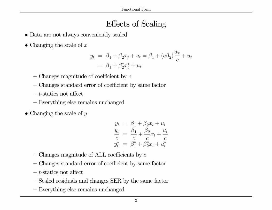
Effects of Scaling• Data are not always conveniently scaled• Changing the scale of

= 1 + 2 + = 1 + (2)+

= 1 + ∗2∗ +

— Changes magnitude of coefficient by — Changes standard error of coefficient by same factor— -statics not affect

— Everything else remains unchanged

• Changing the scale of = 1 + 2 + =

1+2 +

∗ = ∗1 + ∗2 + ∗

— Changes magnitude of ALL coefficients by — Changes standard error of coefficient by same factor— -statics not affect

— Scaled residuals and changes SER by the same factor— Everything else remains unchanged

2

Functional Form

Dummy Variables• Example: E ( |). Equivalent ways to model this:

— Define a dummy variable

1 =

½1 female0 male

Thus, = 0 + 11 + . 0 = E ( |) and 0 + 1 = E ( |)

— Alternatively, define the variable

2 =

½0 female1 male

Thus, = 0 + 12 + . 0 = E ( |) and 0 + 1 = E ( |)

— Or = 11 + 22 + . 1 = E ( |) and 2 = E ( |)

• Standard mistake: include an intercept, 1 and 2. Perfectly collinear (1 + 2 = 1)

• If equation of interest is E ( |): = 0 + 11 + 2 +

• Intercept effect for gender but return on education is the same• A regression model allowing for slope differences (interactions) is

= 0 + 11 + 2 + 31 +

3

Functional Form

Dummy Variables• It is interesting to see how our estimators algebraically handle dummy variables

= 11 +22 +

• By construction 012 = 0. Thus,

b1 = (011)

−101 =

P=1 1P=1 1

=1

1

X=1

1 = 1

bV ³b´ = b2 ∙ (011)

−1 0

0 (022)

−1

¸=

" b21

0

0 b22

#

b2 = 1

X=1

b2• Another candidate for the variance-covariance estimate is

V³b´ = ∙ b21 (0

11)−1 0

0 b22 (022)

−1

¸=

" b211

0

0 b222

#

b2 = 1

X=1

b2 for = 1 2

4

Functional Form

Time Trend• Many economic variables exhibit trends

• Consider a series growing at a constant rate:

= 0 (1 + )

where is the rate of growth per period

• Taking logs (ln) of both sides:

ln = ln 0 + ln (1 + )

• Adding a shock and changing notation:

= 1 + 2 +

where = ln 1 = ln 0 2 = ln (1 + ) '

• Easily checked by taking the first difference and ignoring the disturbance:

∆ = 2

• Important: choice of unit for is irrelevant if it used consistently

5

Functional Form

Seasonality• Economic time series: = + + +

= 0 + 11 + 22 + 33 + 4 +

• E ( |First quarter) = 0 + 1 + 4; E ( |Fourth quarter) = 0 + 4.

• Seasonally adjusted series

∗ = −³b11 + b22 + b33´ (1)

4.4

4.6

4.8

5.0

5.2

5.4

87 88 89 90 91 92 93 94 95 96 97

GDP Seasonally Adjusted GDP

Figure 1: Use of Quarterly Dummies

• Detrended6

Functional Form

Nonlinearity in Regressors

• We are interested in E ( |) = () ∈ R and form of is unknown

• Common approach: polynomial approximation:

= 0 + 1 + 22 + · · · +

+

• Let =¡0 1 · · ·

¢and =

³1

2 · · ·

´ this is = 0 + which is LRM.

Typically, is kept small

• If ∈ R2, a simple quadratic approximation is

= 0 + 11 + 22 + 321 + 4

22 + 512 +

• As dimensionality increases, approximations become non-parsimonious

• Most applications use quadratic terms, some add cubics without interactions (or neural nets,Fourier series, splines, wavelets, etc):

= 0 + 11 + 22 + 321 + 4

22 + 512 + 6

31 + 7

32 +

• Since nonlinear models are linear in parameters, they can be estimated by OLS, and inferenceis conventional

7

Functional Form

Nonlinearity in Regressors

• However, model is nonlinear, so interpretation must take this into account

• For example, in cubic model, slope with respect to 1 isE ( |)

1= 1 + 231 + 52 + 36

21

which is a function of 1 and 2, making reporting of the “slope” difficult

• Important to report slopes for different values of the regressors, chosen to illustrate the pointof interest

• In other applications, average slope may be sufficient. Two obvious candidates:

— Derivative evaluated at sample averages

E ( |)1

¯̄̄̄=

= 1 + 231 + 52 + 3621

— and average derivative

1

X=1

E ( |)1

= 1 + 231 + 52 + 361

X=1

21

8

Functional Form

Transformations

• Even simplest model usually considers nonlinearities

— Example: Cobb-Douglas production function

=

(2)

• Take logs to (2): = + +

• Or: = 0+

• Instances in which no transformation can be used: CES:

=£

+ (1− )

¤1 +

• OLS cannot be applied (NLLS)

9

Functional Form

Some Useful Functions

• Choice of functional form affects interpretation of results

• Use of good analytic skills and experience

Name Function Slope= ElasticityLinear = 1 + 2 2 2

Quadratic = 1 + 22 22 22

2

Cubic = 1 + 23 32

2 323

Log-log ln = 1 + 2 ln 2 2

Log-linear ln = 1 + 2 2 2Linear-log = 1 + 2 ln 2

1 2

1

• If ln is used 0 is required

10

Functional Form

ln ( ) versus as Dependent Variable

• Econometrician can estimate = b+b or ln( ) = b+b (or both). Which is preferable?• Plain truth: either is fine, in the sense that E ( |) and E (ln () |) are well-defined (solong as 0)

• To select one specification over the other, requires the imposition of additional structure (asconditional expectation is linear in , and ∼ N

¡0 2

¢)

• Some good reasons for preferring the ln ( ) over regression

— E (ln () |) may be roughly linear in , while E ( |) may be nonlinear, and linearmodels are easier to report and interpret

— = ln () − E (ln () |) may be less heteroskedastic than the errors from the linearspecification (although the reverse may be true!)

— As long as 0, range of\ln () is well-defined in R; this is not the case for b whichfor some values of b may produce b 0 (Tobit)

— If distribution of is skewed, E ( |) may not be a useful measure of central tendency,and estimates will be influenced by extreme observations (“outliers”); ln E (ln () |)may be a better measure of central tendency, and more interesting to estimate andreport

• Careful when the ln specification is used if interested in obtaining E ( |); Jensen inequality:exp [E (ln () |)] 6= E [exp (ln () |)]

11

Functional Form

Testing for Omitted Nonlinearity• Simple test: add nonlinear functions of , and test significance

— Let = () denote nonlinear functions of . Fit = 0e + 0e + e by OLS, and

test H0 : = 0

• Ramsey RESET test. The null model is = 0 +

=

⎛⎝ b2...b⎞⎠

= 0e + 0e + e (3)

by OLS, and form the Wald statistic ∼ 2−1 for H0 : = 0

— Typically = 2 3 or 4 seem to work best.— Works well as test of functional form against smooth alternatives. Powerful at detectingsingle-index models of the form

= (0) +

where (·) is a smooth “link” function. To see why this is the case, note that (3) maybe written as

= 0e + ³0b´2 e1 + ³0b´3 e2 + · · · + ³0b´ e−1 + e

which has essentially approximated (·) by a -th order polynomial12

Functional Form

Are Errors Normally Distributed?

• Normality of is not crucial for desired properties of OLS estimator (including inference)• However, it leads to use of exact distribution in small samples, helps in forecast, etc• Jarque-Bera test: most popular test for normality

=

6

"2 +

( − 3)2

4

#→ 22

— (Skewness) is a measure of asymmetry of the distribution around the mean

=1

X=1

µ −

¶3= =

1

X=1

µe

¶3 = 0 symmetric, 0 long right tail, 0 long left tail

— (Kurtosis) measures the peakedness or flatness of the distribution

=1

X=1

µ −

¶4= =

1

X=1

µe

¶3 = 3 (normal), 3 peaked (leptokurtic), 3 flat (platykurtic) relative to normal

• Important, if ln ∼ N¡ 2

¢, is log-normal

E = +052

Median () = V = 2+2³2 − 1

´13

Functional Form

Measurement Errors

∗ = ∗ +

∗ or ∗ not observed, = ∗ + = ∗ + ; ∼¡0 2

¢, ∼

¡0 2

¢• Consider first ∗ is observed with error. Then

= ∗ + + = ∗ + ∗; ∗ = +

Model satisfies assumptions of , b unbiased and efficient (not as efficient as when ∗

is observed)

• Now consider ∗ is measured with error,

∗ = ( − ) + = + ∗

where ∗ = − . Since = ∗ + , regressor is correlated with the disturbance, giventhat

Cov (∗) = Cov (∗ + − ) = −2violates assumption of no correlation between and error term. b biased and inconsistent.

• Assumption that measurement errors are unsystematic is naive

• If they are systematic, b may be biased and inconsistent even in the first case14

Functional Form

Omitted Variables

Correct Model: = 11 +22 +

Estimated Model: = 11 +

b1 = ( 011)

−1 01

= 1 + (011)

−1 0122 + (

011)

−1 01

E³b1´ = 1 + (

011)

−1 012| {z }

2

• Each column of is column of slopes of regression of 2 on 1. b1 will generally be biased• Unbiased if either: = 0 which states that 1 and 2 are orthogonal or 2 = 0

• Direction of bias difficult to assess in the general case; consider 1 and 2 are scalars

E³b1´ = 1 +

Cov (1 2)

V (1)2

• If sgn(Cov (1 2)2) 0, E³b1´ 1 and estimator will overestimate effect of 1 on

(Friedman: Permanent Income)

15

Functional Form

Omitted Variables

V³b1 |1

´= 2 ( 0

11)−1

• If we had estimated the “correct” model, E³b∗1´ = 1 and V

³b∗1 |1 2

´would be upper

left block of 2 ( 0)−1, with =£1 2

¤V³b∗1 |´ = 2 ( 0

121)−1

• To compare both expressions, analyze their inverseshV³b1 |1

´i−1−hV³b∗1 |´i−1 = −2

h 012 (

022)

−1 021

i(4)

which is p.d.!

• We may be inclined to conclude that although b1 is biased it has a smaller variance than b∗1• Nevertheless, 2 is not known and needs to be estimated

16

Functional Form

Omitted Variables• Proceeding as usual (thinking that the estimated model is correct) we would obtain

e2 = b0b − 1

but b =1 =1 (11 +22 + ) =122 +1. Then

E (b0b) = 0202122 + 2tr (1)

= 0202122 + 2 ( − 1)

• First term: population counterpart to increase in due to dropping 2. As this term ispositive, e2 will be biased upward (the true variance is smaller). Unfortunately, to take intoaccount this bias we would require to know 2.

• In conclusion

— If we omit relevant variable, b1 and e2 are biased— Even when b1 may be more precise than b∗1, 2 cannot estimate consistently— Only case in which b1 would be unbiased is if 1 and 2 were orthogonal

17

Functional Form

Irrelevant Variables

Correct Model: = 11 +

Estimated Model: = 11 +22 +

b1 = ( 0121)

−1 012 = 1 + (

0121)

−1 012

E³b´ = E " b1b2

#=

∙10

¸; E

¡e2¢ = E µ b0b − 1 − 2

¶= 2

• What is the problem? “Overfit”!! Cost: reduction in precision. Recallb1 = 1 + (0121)

−1 012

V³b1 |´ = 2 ( 0

121)−1

• But variance of b1 is larger than if correct model were estimated:V³b∗1 |1

´= 2 ( 0

11)−1

• Asymptotically as efficient if 1 and 2 orthogonal

• If 1 2 highly correlated, including 2 greatly inflate variance

18

Functional Form

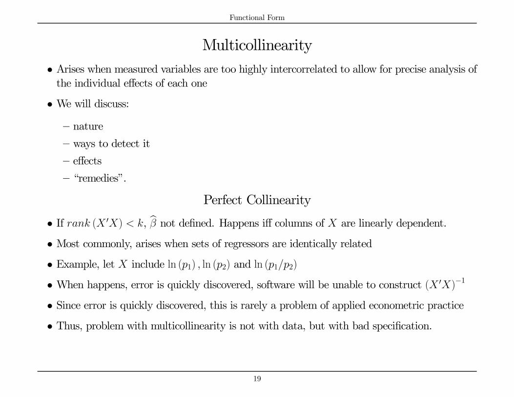
Multicollinearity• Arises when measured variables are too highly intercorrelated to allow for precise analysis ofthe individual effects of each one

• We will discuss:

— nature

— ways to detect it

— effects

— “remedies”.

Perfect Collinearity

• If ( 0) , b not defined. Happens iff columns of are linearly dependent.

• Most commonly, arises when sets of regressors are identically related

• Example, let include ln (1) ln (2) and ln (12)

• When happens, error is quickly discovered, software will be unable to construct ( 0)−1

• Since error is quickly discovered, this is rarely a problem of applied econometric practice

• Thus, problem with multicollinearity is not with data, but with bad specification.

19

Functional Form

Near Multicollinearity

• In contrast to perfect collinearity, near multicollinearity is statistical “problem”

• Problem is not identification but precision

• The higher the correlation between regressors, the less precise will be the estimates

• Troubling about definition of “problem” is that our complaint is with the sample that wasgiven to us!

• The usual “symptoms” of the “problem” are:

— Small changes in data produce wide swings in estimates

— statistics are not significant, 2 is high (excuse?)

— Coefficients have wrong sign or implausible magnitudes

• Problem arises when 0 is “near singular” and columns of are close to linear dependence(loose)

• One implication of near singularity is that numerical reliability of calculations is reduced(more likely that reported calculations will be in error due to floating-point calculationdifficulties)

20

Functional Form

Near Multicollinearity

• Problem is with ( 0)−1, -th diagonal is ( = 1 for convenience):

(0121)−1=³011 − 012 (

022)

−1 021´−1

=

Ã011

Ã1− 012 (

022)

−1 021

011

!!−1=¡011

¡1−21

¢¢−1=

1

011 (1−21)

21 is (uncentered) 2 of regression of 1 on the other regressors. Thus,

V³b1´ = 2

011 (1−21)

if a set of regressors is highly correlated to 1, 21 →1 and V³b1´→∞

21

Functional Form

Detection

• Rule of thumb: concerned when overall 2 any 2• Alternative measure (Belsley) based on the conditioning number ()

=

rmaxmin

’s eigenvalues of = ( 0) =diag³1q0

´

=

⎡⎢⎢⎢⎢⎢⎣1√011

0 · · · 0

0 1√022

0 ...... 0 . . . 0

0 · · · 0 1√0

⎤⎥⎥⎥⎥⎥⎦• If regressors are orthogonal (2 = 0 ∀), = 1. Higher intercorrelation, higher conditioningnumber. If perfect collinearity, min = 0, and →∞

• Belsley suggests 20 indicate potential problems

• Approaches used to deal with “problem”:

— Reduce dimension of (drop variables). Obvious problem: omitted relevant variables,b biased— Principal components, Ridge Regression

22

Functional Form

Bottom Line

• There is no pair of words that is more misused than “multicollinearity problem”

• That explanatory variables are highly collinear is a fact of life

• It is clear that there are realizations of 0 which would be much preferred to the actualdata

• To complaint about the apparent malevolence of nature is not constructive

• Ad-hoc cures for a “bad” sample, can be disastrously inappropriate

• Better to rightly accept the fact that non-experimental data is sometimes not very informa-tive about parameters of interest

23

Functional Form

Bottom Line

• Example to clarify what we are really talking about

— Consider = 11 + 22 +

— A regression of 2 on 1 yields 2 = b1 + b, where b (by construction) is orthogonalto 1

— Substitute this auxiliary relationship into the original one to obtain the model

= 11 + 2

³b1 + b´ +

=³1 + 2b´1 + 2b +

= 11 + 22 +

where 1 =³1 + 2b´ 2 = 2 1 = 1 and 2 = 2 − b1

— Researcher who used 1 and 2 and the parameters 1 and 2, reports that 2 is estimatedinaccurately because of the collinearity problem

— Researcher who happened to stumble on the model with variables 1 and 2 and parame-ters 1 and 2 would report that there is no collinearity problem because 1 and 2 areorthogonal (recall that 1 and b are orthogonal by construction). This researcher wouldnonetheless report that 2(= 2) is estimated inaccurately, not because of collinearity,but because 2 does not vary adequately

24

Functional Form

Bottom Line

• Example illustrates that collinearity as a cause of weak evidence is indistinguishable frominadequate variability as a cause of weak evidence

• In light of that fact, surprising that all econometrics texts have sections dealing with the“collinearity problem” but none has a section on the “inadequate variability problem”

• In summary

— Collinearity is bound to be present in applied econometric practice

— There is no simple solution to this “problem”

— Fortunately, multicollinearity does not lead to errors in inference

— Asymptotic distribution is still valid. Estimates are asymptotically normal, and esti-mated standard errors are consistent

— Confidence intervals are not misleading. They are large, correctly indicating inherentuncertainty about the true parameter values

25

Functional Form

Influential Analysis• OLS seeks to prevent few large residuals at expense of incurring into many relatively smallresiduals

• A few observations can be extremely influential in the sense that dropping them from sample,changes elements of b substantially

• A systematic way to find those influential observations is: let b() OLS estimate of thatwould be obtained if -th observation were omitted

• The key equation is b() − b = −µ 1

1−

¶( 0)

−1b (5)

≡ 0 (0)

−1

which is -th diagonal element of . It is easy to show that

0 ≤ ≤ 1 andX=1

= (6)

so equals on average.

• What should be done with influential observations? Keep or drop?

26

Functional Form

-0.2

-0.1

0.0

0.1

0.2

0.00 0.05 0.10 0.15 0.20

Policy Rate

Gro

wth

1998:09

-0.2

-0.1

0.0

0.1

0.2

0.02 0.04 0.06 0.08 0.10 0.12

Policy Rate

Gro

wth

0.0

0.1

0.2

0.3

0.00 0.05 0.10 0.15 0.20

Policy Rate

p

1998:09

Figure 2: Monetary Policy Rate, Growth, and

27

Functional Form

Model Selection• We discussed costs and benefits of inclusion/exclusion of variables

• How to select specification, when theory does not provide complete guidance?

• This is the question of model selection

— Question: “What is the right model for ?” not well posed, it does not make clear theconditioning set

— Question: “Which subset of (1 · · · ) enters the E ( |1 · · · )?” is well posed.

• In cases, model selection reduced to compare two nested models

= 11 +22 +

1 is × 1 and 2 is × 2. Compare

M1 : = 11 +

M2 : = 11 +22 +

28

Functional Form

Model SelectionM1 : = 11 +

M2 : = 11 +22 +

• Note thatM1 ⊂M2

• We say thatM2 is true if 2 6= 0

• M1 andM2 are estimated by OLS, with residuals b1 and b2, estimated variances b21 andb22, etc., respectively• Model selection procedure is a data-dependent rule which selects one of the models (cM)

• Desirable properties for model selection procedure: consistency

Prh cM =M1 |M1

i→ 1

Prh cM =M2 |M2

i→ 1

29

Functional Form

Selection Based on Fit

• Natural measures of the fit of a regression are

— (b0b)— 2 = 1− (b0b) b2— Gaussian log-likelihood

³b b2´ = − (2) ln b2 + ( is a constant)

• It might be thought attractive to base model selection on one of these measures of fit

• Problem: measures are monotonic between nested models, b01b1 ≥ b02b2 21 ≤ 22 and1 ≤ 2, so M2 would always be selected, regardless of the actual data and probabilitystructure

• Clearly an inappropriate decision rule!

30

Functional Form

Selection Based on Testing

• Common approach to model selection: base decision on statistical test such as Wald

=

µb21 − b22b22¶

• Model selection rule is: for a critical level , let satisfy Pr£22

¤. Select M1 if

≤ , else selectM2.

• Major problem with this approach is that critical level is indeterminate

• Reasoning which helps guide choice of in hypothesis testing (controlling Type I error) isnot relevant for model selection. If is set to be a small number, then Pr

h cM =M1 |M1

i≈

1 − but Prh cM =M2 |M2

icould vary dramatically, depending on the sample size, etc.

Another problem is that if is held fixed, model selection procedure is inconsistent, as

Prh cM =M1 |M1

i→ 1− 1

31

Functional Form

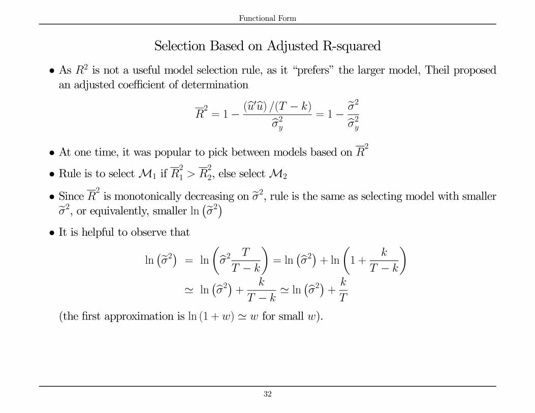
Selection Based on Adjusted R-squared

• As 2 is not a useful model selection rule, as it “prefers” the larger model, Theil proposedan adjusted coefficient of determination

2= 1− (b0b) ( − )b2 = 1− e2b2

• At one time, it was popular to pick between models based on 2

• Rule is to selectM1 if 21

22, else selectM2

• Since 2 is monotonically decreasing on e2, rule is the same as selecting model with smallere2, or equivalently, smaller ln ¡e2¢• It is helpful to observe that

ln¡e2¢ = ln

µb2

−

¶= ln

¡b2¢ + lnµ1 +

−

¶' ln

¡b2¢ +

− ' ln

¡b2¢ +

(the first approximation is ln (1 + ) ' for small ).

32

Functional Form

Selection Based on Adjusted R-squared

• Selecting based on 2is the same as selecting based on ln

¡b2¢ + , which is a particular

choice of penalized likelihood criteria

• It turns out that model selection based on any criterion of the form

ln¡b2¢ +

0 (7)

is inconsistent, as the rule tends to overfit. Indeed, since underM1,

¡ln b21 − ln b22¢ ' ∼ 22 (8)

Prh cM =M1 |M1

i= Pr

h21

22 |M1

i' Pr

£ ln

¡e21¢ ln¡e22¢ |M1

¤' Pr

£ ln

¡b21¢ + 1 ln¡b22¢ + (1 + 2) |M1

¤= Pr [ 2 |M1 ]

→ Pr£22 2

¤ 1

33

Functional Form

Selection Based on Information CriteriaAkaike Information Criterion

• Akaike proposed an information criterion which takes the form

= −2+ 2

which with a Gaussian log-likelihood can be approximated by (7) with = 2:

' ln¡b2¢ + 2

• Imposes larger penalty on overparameterization than does 2

• Rule: selectM1 if 1 2, else selectM2

• Since takes the form (7), it is inconsistent model selection criterion, and tends to overfit

34

Functional Form

Selection Based on Information CriteriaSchwarz Criterion

• Modification of : Schwarz (based on Bayesian arguments)

= −2+

ln ( )

which with a Gaussian log-likelihood can be approximated by

' ln¡b2¢ +

ln ( )

• Since ln ( ) 2 (if 8), places larger penalty than on number of estimatedparameters (is more parsimonious)

• is consistent. Indeed, since (8) holds underM1,

ln ( )→ 0

Prh cM =M1 |M1

i= Pr [1 2 |M1 ]

= Pr [ 2 ln ( ) |M1 ]

= Pr

∙

ln ( ) 2 |M1

¸→ Pr (0 2 |M1) = 1

35

Functional Form

Selection Based on Information CriteriaSchwarz Criterion

• Also underM2, one can show that

ln ( )→∞

Prh cM =M2 |M2

i= Pr [2 1 |M2 ]

= Pr

∙

ln ( ) 2 |M2

¸→ 1

36

Functional Form

Selection Based on Information CriteriaHannan-Quinn Criterion

• Another popular model selection criterion is:

= −2+ 2

ln (ln ( ))

which with a Gaussian log-likelihood can be approximated by

' ln¡b2¢ + 2

ln (ln ( ))

• Since ln (ln ( )) 1 (if 15), places larger penalty than on number ofestimated parameters and is more parsimonious

• As 2 ln (ln ( )) ln ( ) (∀ 0), places a larger penalty than the and selectsmore parsimonious models

• is consistent

37

Functional Form

Selection Based on Information CriteriaA Final Word of Caution

• Results were obtained in OLS context with Gaussian innovations

• To compare different models, dependent variable and sample size need to be the same

• Which model selection criterion is “best”? Open question and an active field of research

• While consistency is desirable, there may be cases in which more parsimonious models runthe risk of excluding relevant variables and that is why some researchers prefer whichis consistent and not as parsimonious as

• From a practical standpoint, it is important to look at the three criteria. Who knows, theymay all choose the same the model!

38

Functional Form

Selection Among Multiple Regressors

• Selection among multiple regressors

= 11 + 22 + · · · + +

which regressors enter the regression?

— Ordered case (Nested):

M1 : 1 6= 0 2 = 3 = · · · = = 0

M2 : 1 6= 0 2 6= 0 3 = · · · = = 0...M : 1 6= 0 2 6= 0 3 6= 0 · · · 6= 0

which are nested. Selection model that minimizes criterion

— Unordered case: 2 models. Example, 210 = 1024 and 220 = 1 048 576. Computationallydemanding

39

Functional Form

Specification Searches• Theory often vague about relationship between variables• Result, many relations established from empirical regularities• If not accounted for, practice can generate serious biases in inference• Names: Data mining, data snooping, data grubbing, data fishing• Examples:

“Because of space limitations, only the best of a variety of alternative models arepresented here.”“The precise variables included in the regression were determined on the basis of

extensive experimentation (on the same body of data).”“Since there is no firmly validated theory, we avoided a priori specification of the

functions we wished to fit.”“We let the data specify the model.”

• Newsletter scam• Conventional hypothesis testing valid when a priori considerations rather than exploratorydata mining determine set of variables included

• When miner uncovers t-statistics that appear significant at 0.05 level by running a largenumber of alternative regressions on the same body of data, the probability of Type I erroris much greater than claimed 5%

40